Embed Size (px)
Citation preview
Supersymmetry and Extra Dimensions
Flip Tanedo
LEPP, Cornell UniversityIthaca, New York
A pedagogical set of notes based on lectures by Fernando Quevedo, Adrian Signer,
and Csaba Csaki, as well as various books and reviews.
Last updated: January 9, 2009

ii
iii
Abstract
This is a set of combined lecture notes on supersymmetry and extra
dimensions based on various lectures, textbooks, and review articles.
The core of these notes come from Professor Fernando Quevedo’s 2006-
2007 Lent Part III lecture course of the same name [1].

iv
v
Acknowledgements
Inspiration to write up these notes in LATEX came from Steffen Gielen’s excel-
lent notes from the Part III Advanced Quantum Field Theory course and the 2008
ICTP Introductory School on the Gauge Gravity Correspondence. Notes from Profes-
sor Quevedo’s 2005-2006 Part III Supersymmetry and Extra Dimensions course exist in
TEXform due to Oliver Schlotterer. The present set of notes were written up indepen-
dently, but simliarities are unavoidable. It is my hope that these notes will provide a
broader pedagogical introduction supersymmetry and extra dimensions.

vi
vii
Preface
These are lecture notes. Version 1 of these notes are based on Fernando Quevedo’s
lecture notes and structure. I’ve also incorporated some relevant topics from my research
that I think are important to round-out the course. Version 2 of these notes will also
incorporate Csaba Csaki’s Advanced Particle Physics notes.
Framed text. Throughout these notes framed text will include parenthetical dis-
cussions that may be omitted on a first reading. They are meant to provide a broader
picture or highlight particular applications that are not central to the main purpose
of the chapter.
The wise men of physics leave behind notes and lectures that are able to convey
insight with fantastic economy. In contrast, for the oaf who put together these notes
(but certainly not the teachers from whom he learned the subject), subtlety would come
at the cost of clarity. Thus I apologize in advance for erring on the side of loquaciousness
in an attempt to overcome my own tentative grasp of the subjects henceforth.

viii
Contents
1 Introduction and History 3
1.1 Prerequisite knowledge . . . . . . . . . . . . . . . . . . . . . . . . . . . . 4
1.2 Heuristic motivation . . . . . . . . . . . . . . . . . . . . . . . . . . . . . 4
1.3 Experimental prospects . . . . . . . . . . . . . . . . . . . . . . . . . . . . 4
1.4 Theoretical prospects . . . . . . . . . . . . . . . . . . . . . . . . . . . . . 4
1.5 The plan . . . . . . . . . . . . . . . . . . . . . . . . . . . . . . . . . . . . 4
2 The Poincare Algebra and its Representations 5
2.1 Poincare Symmetry and Spinors . . . . . . . . . . . . . . . . . . . . . . . 5
2.2 Properties of the Poincare Group . . . . . . . . . . . . . . . . . . . . . . 6
2.2.1 Algebra of the Poincare Group . . . . . . . . . . . . . . . . . . . . 6
2.2.2 The Lorentz Group is related to SU(2)×SU(2) . . . . . . . . . . 7
2.2.3 The Lorentz group is isomorphic to SL(2,C)/Z2 . . . . . . . . . . 8
2.3 Representations of SL(2,C) . . . . . . . . . . . . . . . . . . . . . . . . . 12
2.4 Invariant Tensors . . . . . . . . . . . . . . . . . . . . . . . . . . . . . . . 13
2.5 Contravariant representations . . . . . . . . . . . . . . . . . . . . . . . . 14
2.6 Lorentz-Invariant Spinor Products . . . . . . . . . . . . . . . . . . . . . . 16
2.7 Vector-like Spinor Products . . . . . . . . . . . . . . . . . . . . . . . . . 18
2.8 Generators of SL(2,C) . . . . . . . . . . . . . . . . . . . . . . . . . . . . 19
2.9 Chirality . . . . . . . . . . . . . . . . . . . . . . . . . . . . . . . . . . . . 20
2.10 Fierz Rearrangement . . . . . . . . . . . . . . . . . . . . . . . . . . . . . 21
2.11 Connection to Dirac Spinors . . . . . . . . . . . . . . . . . . . . . . . . . 22
3 The SUSY Algebra 25
3.1 The Supersymmetry Algebra . . . . . . . . . . . . . . . . . . . . . . . . . 25
3.1.1 [Qα,Mµν ] = i(σµν) β
α Qβ . . . . . . . . . . . . . . . . . . . . . . . 27
3.1.2 [Qα, Pµ] = 0 . . . . . . . . . . . . . . . . . . . . . . . . . . . . . . 28
ix
x Contents
3.1.3 Qα, Qβ = 0 . . . . . . . . . . . . . . . . . . . . . . . . . . . . . 29
3.1.4 Qα, Qβ = 2(σµ)αβPµ . . . . . . . . . . . . . . . . . . . . . . . . 29
3.1.5 Commutators with Internal Symmetries . . . . . . . . . . . . . . 30
3.1.6 Extended Supersymmetry . . . . . . . . . . . . . . . . . . . . . . 31
4 Representations of Supersymmetry 33
4.1 Representations of the Poincare Group . . . . . . . . . . . . . . . . . . . 33
4.1.1 Massive Representations . . . . . . . . . . . . . . . . . . . . . . . 35
4.1.2 Massless Representations . . . . . . . . . . . . . . . . . . . . . . . 35
4.2 N = 1 SUSY . . . . . . . . . . . . . . . . . . . . . . . . . . . . . . . . . 36
4.2.1 Massless Multiplets . . . . . . . . . . . . . . . . . . . . . . . . . . 37
4.2.2 Massive Multiplets . . . . . . . . . . . . . . . . . . . . . . . . . . 41
4.2.3 Equality of Fermionic and Bosonic States . . . . . . . . . . . . . . 44
4.2.4 Massless N > 1 Representations . . . . . . . . . . . . . . . . . . . 45
4.2.5 Massive N > 1 Representations with ZAB = 0 . . . . . . . . . . . 49
4.2.6 Massive N > 1 Representations with ZAB 6= 0 . . . . . . . . . . . 50
5 Superfields and Superspace 53
5.1 Coset spaces . . . . . . . . . . . . . . . . . . . . . . . . . . . . . . . . . . 54
5.2 The Calculus of Grassmann Numbers . . . . . . . . . . . . . . . . . . . . 56
5.2.1 Scalar Grassmann Variable . . . . . . . . . . . . . . . . . . . . . . 56
5.2.2 Spinor Grassmann Variables . . . . . . . . . . . . . . . . . . . . . 58
5.3 N = 1 Superfields . . . . . . . . . . . . . . . . . . . . . . . . . . . . . . . 61
5.3.1 Expansion of N = 1 Superfields . . . . . . . . . . . . . . . . . . . 61
5.3.2 SUSY Differential Operators . . . . . . . . . . . . . . . . . . . . . 62
5.3.3 Differential Operators as a Motion in Superspace . . . . . . . . . 65
6 SUSY Breaking 69
6.1 ... . . . . . . . . . . . . . . . . . . . . . . . . . . . . . . . . . . . . . . . . 69
7 XD Basics 71
7.1 Notation and conventions used in this document . . . . . . . . . . . . . . 71
7.2 Notes . . . . . . . . . . . . . . . . . . . . . . . . . . . . . . . . . . . . . . 71
8 Philosophy of Extra Dimensions 73
8.1 5D as EFT . . . . . . . . . . . . . . . . . . . . . . . . . . . . . . . . . . 73
8.2 RS and Holography . . . . . . . . . . . . . . . . . . . . . . . . . . . . . . 73
Contents xi
9 Propagators in Extra Dimensions 75
9.1 Propagators on R5 . . . . . . . . . . . . . . . . . . . . . . . . . . . . . . 75
9.1.1 Scalar Propagator . . . . . . . . . . . . . . . . . . . . . . . . . . . 75
9.1.2 Fermion Propagator . . . . . . . . . . . . . . . . . . . . . . . . . 76
9.1.3 Gauge boson propagator . . . . . . . . . . . . . . . . . . . . . . . 76
9.2 Propagators on R4×S1 . . . . . . . . . . . . . . . . . . . . . . . . . . . . 76
9.2.1 Scalar Propagator . . . . . . . . . . . . . . . . . . . . . . . . . . . 77
9.2.2 Fermion Propagator . . . . . . . . . . . . . . . . . . . . . . . . . 79
9.2.3 Gauge Boson Propagator . . . . . . . . . . . . . . . . . . . . . . . 84
A Literature Guide 85
A.1 General Textbooks . . . . . . . . . . . . . . . . . . . . . . . . . . . . . . 85
A.2 Canonical Reviews . . . . . . . . . . . . . . . . . . . . . . . . . . . . . . 86
A.3 Specialized Reviews . . . . . . . . . . . . . . . . . . . . . . . . . . . . . . 86
A.4 SUSY Breaking . . . . . . . . . . . . . . . . . . . . . . . . . . . . . . . . 86
B Notation and Conventions 87
B.1 Notation and conventions used in this document . . . . . . . . . . . . . . 87
B.2 Blah . . . . . . . . . . . . . . . . . . . . . . . . . . . . . . . . . . . . . . 88
B.3 Comparison with other sources . . . . . . . . . . . . . . . . . . . . . . . 88
B.4 Convention-independent expressions . . . . . . . . . . . . . . . . . . . . . 90
C Useful Identities 91
C.1 Pauli Matrices . . . . . . . . . . . . . . . . . . . . . . . . . . . . . . . . . 91
C.2 Gamma Matrices . . . . . . . . . . . . . . . . . . . . . . . . . . . . . . . 91
C.3 Fierz Identities . . . . . . . . . . . . . . . . . . . . . . . . . . . . . . . . 91
C.4 Miscellaneous . . . . . . . . . . . . . . . . . . . . . . . . . . . . . . . . . 92
D Representations of the Poincare Group 93
D.1 SL(2C) . . . . . . . . . . . . . . . . . . . . . . . . . . . . . . . . . . . . 93
D.2 Projective representations . . . . . . . . . . . . . . . . . . . . . . . . . . 93
D.3 Further Reading . . . . . . . . . . . . . . . . . . . . . . . . . . . . . . . . 93
E Review of Gauge Theories 95
E.1 Lie Algebras . . . . . . . . . . . . . . . . . . . . . . . . . . . . . . . . . . 95
E.2 Comparison with other sources . . . . . . . . . . . . . . . . . . . . . . . 96
F Review of Renormalization and Effective Field Theory 97
xii Contents
F.1 Intuitive picture . . . . . . . . . . . . . . . . . . . . . . . . . . . . . . . . 97
F.2 Understanding UV divergences . . . . . . . . . . . . . . . . . . . . . . . . 97
F.3 Naturalness . . . . . . . . . . . . . . . . . . . . . . . . . . . . . . . . . . 98
Bibliography 103
List of Figures 105
List of Tables 107
Index 108
“The naming of sparticles is a difficult thoughtIt isn’t just one of your grad student gamesYou may think at first I’m mad as a crackpotWhen I tell you, a sparticle has three different names.
First of all, there’s the name we physicists use dailySuch as stop, selectron, photino (twiddle A)Such as higgsino, chargino, sdown, or the LSP,Each of them a sensible physicsy name.
There are fancier names if you think they sound neato,Some are quite playful, some are quite lame:Such as CP-odd Higgs, sneutrino, stau, gravitinoBut all of them sensible physicsy names
But I tell you, a field needs a name that’s particularA name that’s peculiar, and more dignified,Else how can it make its gauge representation much clearerthan to write out its indices, dotting the i’s
Of the names of this kind, I can give you a lot,Such as H-up-j, B-nu, or q-LH-i,Such as g-alpha-sigma, or else twiddle-chi-noughtNames that would make many-an-undergrad cry.
But above and beyond there’s still one name left over,The name that would make even your adviser impressed,The name that no physics research can discover -But the sparticle itself knows, and will never confess.
When you detect a field in profound propagation,There’s only one thing to do that’s worth mention,Time-ordered product, two-point correlation;And compute, and compute, and compute the cross section.
That symmetrically super, supersymmetric,Deep inelastic nonsingular cross section.”
— The Naming of Sparticles (Apologies to TS Eliot)
1

2
Chapter 1
Introduction and History
“Supersymmetry is nearly thirty years old. It seems that now we are ap-
proaching the fourth supersymmetry revolution which will demonstrate
its relevance to nature.”
— G.L. Kane and M. Shifman [2]
Here we go over the basics.
Why SUSY and XD? Both extensions to the SM that evade Coleman-Mandula. Also
they both come together in dualities, e.g. AdS/CFT. Though we won’t get to the AdS
or the CFT sides, we hope to present enough foundational material for SUSY and XD.
3
4 Introduction and History
1.1 Prerequisite knowledge
1.2 Heuristic motivation
1.3 Experimental prospects
1.4 Theoretical prospects
1.5 The plan
We’ll start with SUSY then do XD. If there’s time I’d like to add on some technicolor
and little Higgs stuff later as well.
I should include a broad picture of the program. SUSY requires that we estab-
lish some mathematical machinery before hand, so we’ll start with that. We will first
develop the SUSY algebra as an extension of the Poincare group. Then we will find
representations for this algebra and introduce the superfield notation. Then we’ll do
real stuff.
*** I should say something about the general path. The first few chapters will seem
to be rather abstract and won’t have much connection to the model building that one
might be used to from QFT or SM courses. But these build the necessary formalism to
do SUSY.
Chapter 2
The Poincare Algebra and its
Representations
“I explained the fermion work to my colleague Don Weingarten, and I
remember his answer for he said I was ‘set for life’ !”
— P. Ramond [2]
We will see in subsequent lectures that supersymmetry is inherently connected to
the symmetries of spacetime. Here we briefly review the Poincare group and its spinor
representations. See Appendix D for a more detailed treatment of the Poincare group.
2.1 Poincare Symmetry and Spinors
The Poincare group is given by transformations of Minkowski space of the form
xµ → x′µ = Λµνx
ν + aµ. (2.1)
Here aµ parameterizes translations and Λµν parameterizes transformations of the Lorentz
group containing rotations and boosts. These latter matrices satisfy the relation
ΛTηΛ = η, (2.2)
5
6 The Poincare Algebra and its Representations
where η = diag(+,−,−,−) is the usual Minkowski metric used by particle physicists.
Recall that the Poincare group has four disconnected parts. We specialize to the sub-
group SO(3, 1)↑, i.e. the orthochronous Lorentz group, SO(3, 1)↑ which further
satisfies the constraints
det Λ = +1 (2.3)
Λ00 ≥ 1. (2.4)
This is the part of the Lorentz group that is connected to the identity. Other parts of
the Lorentz group can be obtained from SO(3, 1)↑ by applying the transformations
ΛP = diag(+,−,−,−) (2.5)
ΛT = diag(−,+,+,+). (2.6)
Here ΛP and ΛT respectively refer to parity and time-reversal transformations. It is
worth noting that the fact that the Lorentz group is not simply connected is related to
the existence of a ‘physical’ spinor representation, as we will mention below.
2.2 Properties of the Poincare Group
Let’s review a few important properties of the Poincare group.
2.2.1 Algebra of the Poincare Group
Locally the Poincare group is represented by the algebra
[Mµν ,Mρσ] = i(Mµσηνρ +Mνρηµσ −Mµρηνσ −Mνσηµρ) (2.7)
[P µ, P ν ] = 0 (2.8)
[Mµν , P σ] = i(P µηνσ − P νηµσ). (2.9)
The M are the antisymmetric generators of the Lorentz group,
(Mµν)ρσ = i(δµρ δνσ − δµσδνρ), (2.10)
The Poincare Algebra and its Representations 7
and the P are the generators of translations. As a ‘sanity check,’ one should be able
to recognize in equation (2.7) the usual Euclidean symmetry O(3) by taking µ, ν, ρ, σ ∈1, 2, 3 and noting that at most only one term on the right-hand side survives. equation
(2.8) says that translations commute, while equation (2.9) says that the generators of
translations transform as vectors under the Lorentz group. This is, of course, expected
since the generators of translations are precisely the four-momenta. The factors of i
should also be clear since we’re taking the generators P and M to be Hermitian.
The ‘translation’ part of the Poincare algebra is generally boring. It is the Lorentz
algebra that yields the interesting features of our fields under Poincare transformations.
2.2.2 The Lorentz Group is related to SU(2)×SU(2)
Locally the Lorentz group is related to the group SU(2)×SU(2), i.e. one might sugges-
tively write
SO(3, 1) ≈ SU(2)×SU(2). (2.11)
Let’s flesh this out a bit. One can explicitly separate the Lorentz generators Mµν into
the generators of rotations, Ji, and boosts, Ki:
Ji =1
2εijkMjk (2.12)
Ki = M0i, (2.13)
where εijk is the usual antisymmetric Levi-Civita tensor. We can now define ‘nice’
combinations of these two sets of generators,
Ai =1
2(Ji + iKi) (2.14)
Bi =1
2(Ji − iKi). (2.15)
This may seem like a very arbitrary thing to do, and indeed it’s a priori unmotivated.
However, we can now consider the commutators of these generators,
[Ai, Aj] = i εijk Ak (2.16)
[Bi, Bj] = i εijk Bk (2.17)
[Ai, Bj] = 0. (2.18)
8 The Poincare Algebra and its Representations
Magic! The A and B generators form decoupled representations of the SU(2) algebra.
Note, however, will note that these generators are not Hermitian . Thus we were care-
ful above not to say that SU(3, 1) equals SU(2)×SU(2), where ‘equals’ usually means
either isomorphic or homomorphic. Further, the Lorentz group is not compact (because
of boosts) while SU(2)×SU(2) is. Anyway, we needn’t worry about the precise sense in
which SU(3, 1) and SU(2)×SU(2) are related, the point is that we may label represen-
tations of SU(3, 1) by the quantum numbers of SU(2)×SU(2), (A,B). For example,
a Dirac spinor is in the (12, 1
2) = (1
2, 0) ⊕ (0, 1
2) representation, i.e. the direct sum of
two Weyl reps. (More on this in Section 2.3.) To connect back to reality, the physical
meaning of all this is that we may write the spin of a representation as J = A+B.
So how are SO(3, 1) and SU(2)×SU(2) actually related? We’ve been
deliberately vague about the exact relationship between the Lorentz group and
SU(2)×SU(2). The precise relationship between the two groups are that the com-
plex linear combinations of the generators of the Lorentz algebra are isomorphic to
the complex linear combinations of the Lie algebra of SU(2)×SU(2).
LC(SO(3, 1)) ∼= LC(SU(2)×SU(2)) (2.19)
Be careful not to say that the Lie algebras of the two groups are identical, it is
important to emphasize that only the complexified algebras are identifiable.
2.2.3 The Lorentz group is isomorphic to SL(2,C)/Z2
While the Lorentz group and SU(2)×SU(2) were not related by either a isomorphism
or homomorphism, we can relate the Lorentz group more concretely to SL(2,C). More
precisely, the Lorentz group is isomorphic to the coset space SL(2,C)/Z2
SO(3, 1) ∼= SL(2,C)/Z2 (2.20)
The Poincare Algebra and its Representations 9
Recall that we may represent four-vectors in Minkowski space as complex Hermitian
2× 2 matrices via V µ → Vµσµ, where the σµ are the usual Pauli matrices,
σ0 =
1 0
0 1
σ1 =
0 1
1 0
σ2 =
0 −i
i 0
σ3 =
1 0
0 −1
. (2.21)
To be explicit, we may associate a vector x with either a vector in Minkowski space M4
spanned by the unit vectors eµ,
x = xµeµ, (2.22)
or with a matrix in SL(2,C),
x = xµσµ. (2.23)
For the Minkowski four-vectors, we already understand how a Lorentz transformation
Λ acts on a [covariant] vector xµ while preserving the vector norm1,
|x|2 = x20 − x2
1 − x22 − x2
3. (2.24)
For Hermitian matrices, there is an analogous transformation by the action of the group
of invertible complex matrices of unitary determinant, SL(2,C). For N ∈ SL(2,C),
N†xN is also in the space of Hermitian 2× 2 matrices. Such transformations preserve
the determinant of x,
det x = x20 − x2
1 − x22 − x2
3. (2.25)
The equivalence of the right-hand sides of equations (2.24) and (2.25) are very suggestive
of an identification between the Lorentz group SO(3, 1) and SL(2,C). Indeed, equation
(2.25) implies that for each SL(2,C) matrix N, there exists a Lorentz transformation Λ
such that
N†xµσµN = (Λx)µσµ. (2.26)
1This is the content of equation (2.2), which defines the Lorentz group.
10 The Poincare Algebra and its Representations
We discuss this in more detail in Appendix D, but a very important feature should
already be apparent: the map from SL(2,C) → SO(3, 1) is 2-1. This is clear since
the matrices N and −N yield the same Lorentz transformation, Λµν . Hence it is not
SO(3, 1) and SL(2,C) that are isomorphic, but rather SO(3, 1) and SL(2,C)/Z2.
The point that we should glean from this is that one will miss something if on
only looks at representations of SO(3, 1) and not the representations of SL(2,C). This
‘something’ is the spinor representation. How should we have known that SL(2,C) is the
important group? One way of seeing this is noting that SL(2,C) is simply connected
as a group manifold.
By the polar decomposition for matrices, any g ∈ SL(2,C) can be written as the
product of a unitary matrix U times the exponentiation of a traceless Hermitian matrix
h,
g = Ueh. (2.27)
We may write these matrices explicitly in terms of real parameters a, · · · , g;
h =
c a− ib
a+ ib −c
(2.28)
U =
d+ ie f + ig
−f + ig d− ie
. (2.29)
Here a, b, c are unconstrained while d, · · · , g must satisfy
d2 + e2 + f 2 + g2 = 1. (2.30)
Thus the space of 2× 2 traceless Hermitian matrices h is topologically identical to R3
while the space of unit determinant 2× 2 unitary matrices U is topologically identical
to the three-sphere, S3. Thus we have
SL(2,C) = R3×S3. (2.31)
As both of the spaces on the right-hand side are simply connected, their product,
SL(2,C), is also simply connected. This is a ‘nice’ property because we can write down
any element of the group by exponentiating its generators at the identity. But even fur-
The Poincare Algebra and its Representations 11
ther, since SL(2,C) is simply connected, its quotient space SL(2,C)/Z2 = SO(3, 1) is
not simply connected. We already mentioned this when we introduced the orthochronous
Lorentz group, but the point is that we would like to use simply connected groups to con-
struct our representations (more on this in the box below). Thus we shall use SL(2,C),
not SO(3, 1), for our representations of the Lorentz part of the Poincare group. SL(2,C)
is called the universal covering group of SO(3, 1), meaning that it is the ‘minimal’
simply connected group homeomorphic to SO(3, 1). This universal covering group is
often referred to as Spin(3, 1).
Projective representations and universal covering groups. For the uniniti-
ated, it may not be clear why the above rigamarole is necessary or even interesting.
Here we would like to approach the topic from a different direction to answer, in
words, the question of what the spinor representation is and why it is physical.
A typical “representation theory for physicists” course goes into detail about con-
structing the usual tensor representations of groups but only mentions the spinor
representation of the Lorentz group in passing. Students ‘inoculated’ with a quan-
tum field theory course will not bat an eyelid at this, since they’re already used
to the technical manipulation of spinors. But where does the spinor representation
come from if all of the ‘usual’ representations we’re used to are tensors?
The answer lies in quantum mechanics. Recall that when we write representa-
tions U of a group G, we have U(g1)U(g2) = U(g1g2) for g1, g2 ∈ G. In quan-
tum physics, however, physical states are invariant under phases, so we have
the freedom to be more general with our multiplication rule for representations:
U(g1)U(g2) = U(g1g2) exp(iφ(g1, g2)). Such ‘representations’ are called projective
representations. In other worse, quantum mechanics allows us to use projective
representations rather than ordinary representations.
It turns out that not every group admits ‘inherently’ projective representations. In
cases where such reps are not allowed, a representation that one tries to construct
to be projective can have its generators redefined to reveal that it is actually an
ordinary non-projective representation. It turns out that groups that are not simply
connected, such as the Lorentz group, admit inherently projective representations.
In particular, the Lorentz group is doubly connected, i.e. going over any loop twice
will allow it to be contracted to a point. This means that the phase in the projective
representation must be ± 1. One can consider taking a loop in the Lorentz group that
12 The Poincare Algebra and its Representations
corresponds to rotating by 2π along the z-axis. Representations with a projective
phase +1 will return to their original state after a single rotation, these are the
particles with integer spin. Representations with a projective phase −1 will return
to their original state only after two rotations, and these correspond to spin-1/2
particles, or spinors.
There is an excellent discussion of this in Weinberg, Volume I. We reproduce the main
parts of Weinberg’s argument in Appendix D. More on the representation theory of
the Poincare group and its SUSY extension can be found in Buchbinder and Kuzenko
[3]. Further pedagogical discussion of spinors can be found in [4].
2.3 Representations of SL(2,C)
The representations of the universal cover of the Lorentz group, SL(2,C), are spinors.
Most standard quantum field theory texts do calculations in terms of four-component
Dirac spinors. This has the benefit of representing all the degrees of freedom of a typical
Standard Model massive fermion into a single object. In SUSY, on the other hand,
it will turn out to be natural to work with two-component spinors. For example, a
complex scalar field has two real degrees of freedom. In order to have a supersymmetry
between complex scalars and fermions, we require that the number of degrees of freedom
match for both types objects. A Dirac spinor, however, has four real degrees of freedom
(2× 4 complex degrees of freedom - 4 from the Dirac equation). Thus we argue that
it is more useful to consider Weyl (and later Majorana) spinors with the same number
of degrees of freedom as the complex scalar field that they mix with under SUSY. For
a comprehensive guide to calculating with two-component spinors, see the review by
Dreiner, Haber, and Martin [5].
Let us start by defining the fundamental and conjugate (or antifundamental)
representations of SL(2,C). These are just the matrices N βα and (N∗) β
α . Don’t be
startled by the dots on the indices, they’re just a book-keeping device to keep the
fundamental and the conjugate indices from getting confused. One cannot contract a
The Poincare Algebra and its Representations 13
dotted with an undotted SL(2,C) index; this would be like trying to contract spinor
indices (α or α) with vector indices (µ): they index two totally different representations2.
We are particularly interested in the objects that these matrices act on. Let us thus
define left-handed Weyl spinors, ψ, as those acted upon by the fundamental rep and
right-handed Weyl spinors, χ, as those that are acted upon by the conjugate rep.
Again, do not be startled with the extra jewelry that our spinors display. The bar on the
right-handed spinor just serves to distinguish it from the left-handed spinor. To be clear,
they’re both spinors, but they’re different types of spinors that have different types of
indices and that transform under different representations of SL(2,C). Explicitly,
ψ′α = N βα ψβ (2.32)
χ′α = (N∗) βα χβ. (2.33)
2.4 Invariant Tensors
We know that ηµν is invariant under SO(3, 1) and can be used (along with the inverse
metric) to raise and lower SO(3, 1) indices. For SL(2,C), we can build an analogous
tensor, the unimodular antisymmetric tensor
εαβ = i(σ2)αβ (2.34)
=
0 1
−1 0
. (2.35)
Unimodularity (unit determinant) and antisymmetry uniquely define the above form up
to an overall sign. The choice of sign is a convention. This tensor is invariant under
SL(2,C) since
ε′αβ = ερσN αρ N β
σ (2.36)
= εαβ detN (2.37)
= εαβ. (2.38)
2This doesn’t mean that we can’t swap between different types of indices. In fact, this is exactly whatwe did in equations (2.22) and (2.23). We’ll get to the role of the σ matrices very shortly.
14 The Poincare Algebra and its Representations
We can now use this tensor to raise undotted SL(2C) indices:
ψα ≡ εαβψα. (2.39)
To lower indices we can use an analogous unimodular antisymmetric tensor with two
lower indices. For consistency, the overall sign of the lowered-indices tensor must be
defined as
εαβ = −εαβ. (2.40)
This is to ensure that the upper- and lower-indices tensors are inverses, i.e. so that the
combined operation of raising then lowering an index does not introduce a sign. Dotted
indices indicate the complex conjugate representation, ε∗αβ = εαβ. Since ε is real we thus
use the same sign convention for dotted indices as undotted indices,
ε12 = ε12 = −ε12 = −ε12. (2.41)
So we may raise dotted indices in exactly the same way:
χα ≡ εαβχα. (2.42)
2.5 Contravariant representations
Now that we’re familiar with the ε tensor, we should tie up a loose end from Section
2.3. There we introduced the fundamental and conjugate representations of SL(2,C).
What happened to the contravariant representations that transform under the inverse
matrices N−1 and N∗−1?
It turns out that these representations are equivalent (in the group theoretical sense)
to the fundamental and conjugate representations presented above. Using the antisym-
metric tensor εαβ (ε12 = 1) and the unimodularity of N ∈ SL(2,C),
εαβNαγN
βδ = εγδ detN (2.43)
εαβNαγN
βδ = εγδ (2.44)(
NT) α
γεαβN
βδ = εγδ (2.45)
εαβNβδ =
[(NT)−1] γ
αεγδ (2.46)
The Poincare Algebra and its Representations 15
And hence by Schur’s Lemma N and (NT )−1 are equivalent. Similarly, N∗ and (N †)−1
are equivalent. This is not surprising, of course, since we already knew that the anti-
symmetric tensor, ε, is used to raise and lower indices in SL(2,C). Thus the equivalence
of these representations is no more ‘surprising’ than the fact that Lorentz vectors with
upper indices are equivalent to Lorentz vectors with lower indices. Explicitly, then, the
contravariant representations transform as
ψ′α = ψβ(N−1) αβ (2.47)
χ′α = χβ(N∗−1) α
β. (2.48)
To summarize, our two-component spinor representations are
ψ′α = N βα ψβ (2.49)
χ′α = (N∗) βα χβ (2.50)
ψ′α = ψβ(N−1) αβ (2.51)
χ′α = χβ(N∗−1) α
β. (2.52)
Occasionally one will see equations (2.50) and (2.52) written in terms of Hermitian
conjugates,
χ′α = χβ(N †)βα (2.53)
χ′α = (N †−1)αβχβ. (2.54)
We will not advocate this notation, however, since Hermitian conjugates are a bit delicate
notationally in quantum field theories.
Stars and daggers. Let us clarify some notation. When dealing with classical
fields, the complex conjugate representation is the usual complex conjugate of the
field; i.e. ψ → ψ∗. When dealing with quantum fields, on the other hand, it is
conventional to write a Hermitian conjugate; i.e. ψ → ψ†. This is because the
quantum field contains creation and annihilation operators. This is the same reason
why Lagrangians are often written L = term + h.c. The classical Lagrangian is a
scalar quantity, so in that case one could have just written ‘c.c.’ (complex conjugate)
rather than ‘h.c.’ (Hermitian conjugate). In QFT, however, since the terms in the
16 The Poincare Algebra and its Representations
Lagrangian are composed of quantum fields—which are operators—it is necessary
for them to have a Hermitian conjugate.
It is worth making one further note about notation. Sometimes authors will write
ψα = ψ†α. (2.55)
This is technically correct, but it can be a bit misleading since one shouldn’t get into
the habit of thinking of the bar as some kind of operator. The bar and its dotted
index are notation to distinguish the right-handed representation from the left-handed
representation. The content of the above equation is the statement that the conjugate
of a left-handed spinor transforms as a right-handed spinor.
In light of our previous info box, one might feel like we ought to be very explicit if
the right-hand side of the above equation should have a dagger or a star. Actually, after
spending all that time being pedantic, it doesn’t matter. We know that under a Lorentz
transformation, ψα → (N∗) βα ψβ. This seems awkward if we want to associate ψ with
ψ†. Recall, however, that N ∈ L(SL(2,C)). Elements of the group SL(2,C) have unit
determinant, so elements of the algebra L(SL(2,C)) have the property N = NT . Thus
we may swap N∗ with N † and we may say either ψ = ψ† consistently.
2.6 Lorentz-Invariant Spinor Products
Now that we’re armed with a metric to raise and lower indices, we can also define the
inner product of spinors as the contraction of upper and lower indices. Note that in
order to form inner products that are actually Lorentz-invariant, one cannot contract
dotted and undotted indices.
There is a very nice short-hand that is commonly used in supersymmetry that allows
us to drop contracted indices. Since it’s important to distinguish between left- and right-
handed Weyl spinors, we have to be careful that dropping indices doesn’t introduce an
ambiguity. This is why right-handed spinors are barred in addition to having dotted
The Poincare Algebra and its Representations 17
indices. Let us now define the contractions
ψχ ≡ ψαχα (2.56)
ψχ ≡ ψαχα. (2.57)
Note that the contractions are different for the left- and right-handed spinors. This is a
choice of convention that has been chosen such that
(ψχ)† ≡ (ψαχα)† = χαψα ≡ χψ = ψχ. (2.58)
The second equality is worth explaining. Why is it that (ψαχα)† = χαψα? Recall
from that the Hermitian conjugation acts on the creation and annihilation operators in
the quantum fields ψ and χ. The Hermitian conjugate of the product of two Hermitian
operators AB is given by B†A†. The coefficients of these operators in the quantum fields
are just c-numbers (‘commuting’ numbers), so the conjugate of ψαχα is(χ†)α
(ψ†)α
.
Now let’s get back to our contraction convention. Recall that quantum spinor fields
are Grassmann, i.e. they anticommute. Thus we show that with our contraction con-
vention, the order of the contracted fields don’t matter:
ψχ = ψαχα = −ψαχα = χαψα = χψ (2.59)
ψχ = ψαχα = −ψαχα = χαψ
α= χψ. (2.60)
It is actually rather important that quantum spinors anticommute. If the ψ were
commuting objects, then
ψ2 = ψψ = εαβψβψα = ψ2ψ1 − ψ1ψ2 = 0. (2.61)
Thus we must have ψ such that
ψ1ψ2 = −ψ2ψ1, (2.62)
i.e. the components of the Weyl spinor must be Grassmann. So one way of understand-
ing why spinors are anticommuting is that metric that raises and lowers the indices are
antisymmetric. (We know, of course, that from another perspective this anticommuta-
tivity comes from the quantum creation and annihilation operators.)
18 The Poincare Algebra and its Representations
Finally, we note a handy equality that stems from spinor antisymmetry:
ψαψβ =1
2εαβψψ. (2.63)
2.7 Vector-like Spinor Products
Notice that the Pauli matrices give a natural way to go between SO(3, 1) and SL(2,C)
indices. Using equation (2.26),
(xµσµ)αα → N β
α (xνσν)βγN
∗ γα (2.64)
= (Λ νµ xν)σ
µαα. (2.65)
Then we have
(σµ)αα = N βα (σν)βγ(Λ
−1)µνN∗ γα . (2.66)
One could, for example, swap between the vector and spinor indices by writing
Vµ → Vαβ ≡ Vµ(σµ)αβ. (2.67)
We can define a ‘raised index’ σ matrix,
(σµ)αα ≡ εαβεαβ(σµ)ββ (2.68)
= (σµ)† (2.69)
= (1,−−→σ ). (2.70)
Note the bar and the reversed order of the dotted and undotted indices. The bar is
just notation to indicate the index structure, similarly to the bars on the right-handed
spinors. How do we understand the indices? Let us go back to the matrix form of the
Pauli matrices (2.21) and the upper-indices epsilon tensor (2.35). One may use ε = iσ2
and to directly verify that
εσmu = σTµ ε, (2.71)
The Poincare Algebra and its Representations 19
and hence
σµ = εσTµ εT . (2.72)
Restoring indices on the right-hand side,
εσTµ εT → εαβ(σµT )ββ(εT )βα (2.73)
→ εαβεαβ(σµ)ββ. (2.74)
Thus we see that the σµ have a dotted-then-undotted index structure. A further consis-
tency check comes from looking at the structure of the γ matrices as applied to the Dirac
spinors formed using Weyl spinors with our index convention. We do this in Section 2.9.
2.8 Generators of SL(2,C)
How do Lorentz transformations act on Weyl spinors? We should already have a hint
from the generators of Lorentz transformations on Dirac spinors. (Go ahead and review
this section of your favorite QFT textbook.) The objects that obey the Lorentz algebra,
equation (2.7), and generate the desired transformations are given by the matrices,
(σµν) βα =
i
4(σµσν − σνσµ) β
α (2.75)
(σµν)αβ
=i
4(σµσν − σνσµ)α
β. (2.76)
The assignment of dotted and undotted indices are deliberate; they tell us which gener-
ator corresponds to the fundamental versus the conjugate representation. (The choice
of which one is fundamental versus conjugate, of course, is arbitrary.) Thus the left and
right-handed Weyl spinors transform as
ψα →(e−
i2ωµνσµν
) β
αψβ (2.77)
χα →(e−
i2ωµνσµν
)αβχβ. (2.78)
We can invoke the SU(2)×SU(2) ‘representation’ (and we use that word very
loosely) of the Lorentz group from equations (2.12) and (2.13) to write the σµν gen-
20 The Poincare Algebra and its Representations
erators as
Ji =1
2εijkσjk =
1
2σi (2.79)
Ki = σ0i = −1
2σi, (2.80)
where one then finds
Ai =1
2(Ji + iKi) =
1
2σi (2.81)
Bi =1
2(Ji − iKi) = 0. (2.82)
Thus the left-handed Weyl spinors ψα are (12, 0) spinor representations Similarly, one
finds that the right-handed Weyl spinors χα are (0, 12) spinor representations.
2.9 Chirality
Now let’s get back to a point of nomenclature. Why do we call them left- and right-
handed spinors? The Dirac equation tells us3
pµσµψ = mψ (2.83)
pµσµχ = mχ. (2.84)
Equation (2.84) follows from equation (2.83) via Hermitian conjugation, as appropriate
for the conjugate representation.
In the massless limit, then, p0 → |p| and hence(σ ·p|p|
ψ
)= ψ (2.85)(
σ ·p|p|
χ
)= −χ. (2.86)
3To be clear, there’s some arbitrariness here. How do we know which ‘Dirac equation’ (i.e. with σ orσ) to apply to ψ (the fundamental rep) versus χ (the conjugate rep)? This is convention, ‘by theinterchangeability of the fundamental and conjugate reps’ and ‘the interchangeability of σ and σ’if you wish. Once we have chosen the convention of equation (2.83), then equation (2.84) followsfrom Hermitian conjugation. In other words, once we’ve chosen that the fundamental representationgoes with the ‘σ’ Dirac equation (2.83), we know that the conjugate representation goes with the‘σ† = σ’ Dirac equation (2.84). If you ever get confused, check the index structure of σ and σ andmake sure they are contracting honestly.
The Poincare Algebra and its Representations 21
We recognize the quantity in parenthesis as the helicity operator, and hence ψ has helicity
+1 (left-handed) and χ has helicity -1 (right-handed). Non-zero masses complicate
things, of course. In fact, they complicate things differently depending on whether the
masses are Dirac or Majorana. We’ll get to this in due course, but the point is that even
though ψ and χ are no longer helicity eigenstates, they are chirality eigenstates:
γ5
ψ0
=
ψ0
(2.87)
γ5
0
χ
= −
0
χ
, (2.88)
where we’ve put the Weyl spinors into four-component Dirac spinors in the usual way
so that we may apply the chirality operator, γ5. (See Section 2.11.)
Chirality. Keeping the broad program in mind, let us take a moment to note that
chirality will play an important role in whatever new physics we might find at the
Terascale. The Standard Model is a chiral theory (e.g. qL and qR are in different
gauge representations), so whatever Terascale completion supersedes it must also be
chiral. This is no problem in SUSY where we may place chiral fields into different
supermultiplets (‘superfields’). In XD, however, we run into the problem that there
is no chirality operator in five dimensions. This leads to a lot of subtlety in model-
building that we shall discuss in the second-half of this document.
It is assumed that the reader can distinguish between helicity and chirality. If not,
then s/he is kindly requested to review this for posterity’s sake.
2.10 Fierz Rearrangement
Fierz identities are useful for rewriting spinor operators by swapping the way indices are
contracted. For example,
(χψ)(χψ) = −1
2(ψψ)(χχ). (2.89)
22 The Poincare Algebra and its Representations
One can understand these Fierz identities as an expression of the decomposition of
tensor products in group theory. For example, we could consider the decomposition
(12, 0)⊗ (0, 1
2) = (1
2, 1
2):
ψαχα =1
2(ψσµχ)σµαα, (2.90)
where, on the right-hand side, the object in the parenthesis is a vector in the same sense
as equation (2.67). The factor of 12
is, if you want, a Clebsch-Gordan coefficient.
Another example is the decomposition for (12, 0)⊗ (1
2, 0) = (0, 0) + (1, 0):
ψαχβ =1
2εαβ(ψχ) +
1
2(σµνεT )αβ(ψσµνχ). (2.91)
Note that the (1, 0) rep is the antisymmetric tensor representation. All higher dimen-
sional representations can be obtained from products of spinors. Explicit calculations
can be found in the lecture notes by Muller-Kirsten and Wiedemann [6].
A set of Fierz identities are listed in Section C.3.
2.11 Connection to Dirac Spinors
We would now like to explicitly connect the machinery of two-component Weyl spinors
to the four-component Dirac spinors that we (unfortunately) teach our children.
Let us define
γµ ≡
0 σµ
σµ 0
. (2.92)
This, one can check, gives us the Clifford algebra
γµ, γν = 2ηµν ·1. (2.93)
We can further define the fifth γ-matrix, the four-dimensional chirality operator,
γ5 = iγ0γ1γ2γ3 =
−1 0
0 1
. (2.94)
The Poincare Algebra and its Representations 23
A Dirac spinor is defined, as mentioned above, as the direct sum of left- and right-
handed Weyl spinors, ΨD = ψ ⊕ χ, or
ΨD =
ψαχα
. (2.95)
The choice of having a lower undotted index and an upper dotted index is convention
and comes from how we defined our spinor contractions. The generator of Lorentz
transformations takes the form
Σµν =
σµν 0
0 σµν
, (2.96)
with spinors transforming as
ΨD → e−i2ωµνΣµνΨD. (2.97)
In our representation the action of the chirality operator is given by γ5,
γ5ΨD =
−ψαχα
. (2.98)
We can then define left- and right-handed projection operators,
PL,R =1
2
(1∓ γ5
). (2.99)
Using the standard notation, we shall define a barred Dirac spinor as ΨD ≡ Ψ†γ0. Note
that this bar has nothing to do with the bar on a Weyl spinor. We can then define
a charge conjugation matrix C via C−1γµC = −(γµ)T and the Dirac conjugate spinor
Ψ cD = CΨ
T
D , or explicitly in our representation,
Ψ cD =
χαψα
. (2.100)
24 The Poincare Algebra and its Representations
A Majorana spinor is defined to be a Dirac spinor that is its own conjugate, ΨM = ΨcM .
We can thus write a Majorana spinor in terms of a Weyl spinor,
ΨM =
ψαψα
. (2.101)
It is worth noting that in four dimensions there are no Majorana-Weyl spinors. This,
however, is a dimension-dependent statement, as we will see in Section ***. A good
treatment of this can be found in the appendix of Polchinksi’s second volume [7].
Much ado about dots and bars. It’s worth emphasizing once more that the dots
and bars are just book-keeping tools. Essentially they are a result of not having
enough alphabets available to write different kinds of objects. The bars can be
especially confusing for beginning supersymmetry students since one is tempted to
associate them with the barred Dirac spinors, Ψ = Ψ†γ0. Do not make this mistake.
Weyl and Dirac spinors are different objects. The bar on a Weyl spinor has nothing to
do with the bar on a Dirac spinor, and certainly has nothing to do with antiparticles.
We see this explicitly when we construct Dirac spinors out of Weyl spinors (namely
Ψ = ψ ⊕ χ), but it’s worth remembering because the notation can be misleading.
In principle ψ and ψ are totally different spinors in the same way that α and α
are totally different indices. Sometimes—as we have done above—we may also use
the bar as an operation that converts an unbarred Weyl spinor into a barred Weyl
spinor. That is to say that for a left-handed spinor ψ, we may define ψ = ψ†. To
avoid ambiguity it is customary—as we have also done—to write ψ for left-handed
Weyl spinors, χ for right-handed Weyl spinors, and ψ to for the right-handed Weyl
spinor formed by taking the Hermitian conjugate of the left-handed spinor ψ.
To make things even trickier, much of the literature on extra dimensions use the
convention that ψ and χ (unbarred) refer to left- and right-‘chiral’ Dirac spinors.
Here ‘chiral’ means that they permit chiral zero modes, a non-trivial subtlety of
extra dimensional models that we will get to in due course. For now we’ll use the
‘SUSY’ convention that ψ and χ are left- and right-handed Weyl spinors.
Chapter 3
The SUSY Algebra
“Supersymmetry is nearly thirty years old. It seems that now we are ap-
proaching the fourth supersymmetry revolution which will demonstrate
its relevance to nature.”
— G.L. Kane and M. Shifman [2]
3.1 The Supersymmetry Algebra
Around the same time that the Beatles released Sgt. Pepper’s Lonely Hearts Club Band,
Coleman and Mandula published their famous ‘no-go’ theorem which stated that the
most general symmetry Lie group of an S-matrix in four dimensions is the direct product
of the Poincare group with an internal symmetry group1. In other words, there can be
no mixing of spins within a symmetry multiplet.
Ignorance is bliss, however, and physicists continued to look for extensions of the
Poincare symmetry for some years without knowing about Coleman and Mandula’s
result. in particular, Golfand and Licktmann extended the Poincare group using Grass-
mann operators, ‘discovering’ supersymmetry in physics. Independntly, Ramond, Neveu,
Schwarz, Gervais, and Sakita where applying similar ideas in two dimensions to insert
fermions into a budding theory of strings, hence developing (wait for it...) superstring
theory.
1See Weinberg Vol III for a proof of the Coleman-Mandula theorem.
25
26 The SUSY Algebra
SUSY, then, is able to evade the Coleman-Mandula theorem by generalizing the
symmetry from a Lie algebra to a graded Lie algebra. This has the property that if
Oa are operators, then
OaOb − (−1)ηaηbObOa = iCeabOe, (3.1)
where,
ηa =
0 if Oa is bosonic
1 if Oa is fermionic(3.2)
The Poincare generators P µ,Mµν are both bosonic generators with (A,B) = (12, 1
2), (1, 0)⊕
(0, 1) respectively. In supersymmetry, on the other hand, we add fermionic genera-
tors, QAα , Q
B
α . Here A,B = 1, · · · ,N label the number of supercharges (these are, of
course, different from the (A,B) that label representations of the Lorentz algebra) and
α, α = 1, 2 are Weyl spinor indices. We will primarily focus on simple supersymmetry
where N = 1. We call N > 1 extended supersymmetry.
Haag, Lopouszanski, and Sohnius showed in 1974 that (12, 0) and (0, 1
2) are the only
generators for supersymmetry. For example, it would be inconsistent to include genera-
tors Q in the representation (A,B = (12, 1)). The general argument is that the product
of two spinor generators has to be bosonic and the only bosonic generators are M and
P . A further discussion of this can be found in Weinberg III [8].
Without further ado, let’s write down the supersymmetry algebra.
[Mµν ,Mρσ] = i(Mµνηνρ +Mνρηµσ −Mµρηνσ −Mνσηµρ) (3.3)
[P µ, P ν ] = 0 (3.4)
[Mµν , P σ] = i(P µηνσ − P νηµσ) (3.5)
[Qα,Mµν ] = i(σµν) β
α Qβ (3.6)
[Qα, Pµ] = 0 (3.7)
Qα, Qβ = 0 (3.8)
Qα, Qβ = 2(σµ)αβPµ (3.9)
We’re already familiar with equations (3.3 - 3.5) as being the usual Poincare algebra. It
remains to discuss the remaining equations involving the new fermionic generators.
The SUSY Algebra 27
Before we do that, however, two important notes are in order. First, one should check
that the assignment of commutators in the above equations matches our definition for a
graded Lie algebra, equation (3.1). Second, one should note that up to overall constants,
we should almost have been able to guess the form of the new equations by matching
the index structure on the left- and right-hand sides of each equation, using only the
SUSY algebra and the generators of SL(2,C), equations (2.75) and (2.76).
3.1.1 [Qα,Mµν] = i(σµν) β
α Qβ
Now consider equation (3.6). How do we understand this? First of all, because Qα is a
spinor, we may write down its transformation under an infinitesimal Lorentz transfor-
mation,
Q′α = (e−i2ωµνσσν ) β
α Qβ (3.10)
≈ (1− i
2ωµνσ
µν) βα Qβ. (3.11)
However, Qα also leads a second life as an operator. Thus we know it also transforms
as
Q′α = U †QαU (3.12)
U = e−i2ωµνMµν
, (3.13)
and hence,
Q′α ≈ (1 +i
2ωµνM
µν)Qα (1− i
2ωµνM
µν). (3.14)
Setting equations (3.11) and (3.14) equal to one another,
Qα −1
2ωµν(σ
µν) βα Qβ = Qα −
i
2ωµν(QαM
µν −MµνQα) +O(ω2), (3.15)
from which we finally deduce equation (3.6)
[Qα,Mµν ] = i(σµν) β
α Qβ.
28 The SUSY Algebra
Note that the commutator for the right-handed representation corresponds to placing
bars on this relation,
[Qα,Mµν ] = iεαδ(σ
µν)δβQβ. (3.16)
This follows from the transformation law in equation (2.76).
3.1.2 [Qα, Pµ] = 0
Equation (3.7) tells us that translations don’t affect the fermionic transformations. This
is a bit surprising since our mnemonic of looking at the index structure suggests that
the right-hand side of this equation could be proportional to (σµ)ααQα. Indeed, let us
assume this to find that the proportionality constant, c must be zero. Thus,
[Qα, Pµ] = c(σµ)ααQ
α. (3.17)
This is actually two equations since we can get a corresponding equation for Q. Recall
that taking the Hermitian conjugate of a left-handed spinor operator produces a right-
handed spinor (and vice versa), so that Q †α = Qα. What about the σ matrix? From
equation (2.68) we have (σµ)αα = εαβεαβ(σµ)ββ. Putting this together and taking the
Hermitian conjugate of equation (3.17),
[Q †α , P
µ] = c∗(σµ)ααQα†
(3.18)
[Qα, Pµ] = c∗εαβεαβ(σµ)ββQα (3.19)
[Qα, P µ] = c∗(σµ)βαQα. (3.20)
Note that the Hermitian conjugate acts only on the operator Q, that is to say that there
is no transpose of the σ matrix. Equations (3.17) and (3.20) are, by index structure
(that is, by Lorentz covariance), the most general form of the commutators of Q and Q
with P . To find c we invoke the Jacobi identity for P µ, P ν , and Qα:
0 = [P µ, [P ν , Qα]] + [P ν , [Qα, Pµ]] + [Qα, [P
µ, P ν ]] (3.21)
= −cσναα[P µ, Q
α]
+ cσµαα
[P ν , Q
α]
(3.22)
= |c|2 σµαασναβQβ − |c|2 σναασµαβQβ (3.23)
= |c|2 (σµν) βα Qβ. (3.24)
The SUSY Algebra 29
From this we conclude that c = 0, hence proving our assertion.
3.1.3 Qα, Qβ = 0
Equation (3.8) comes from a similar argument. Again we may write the most general
form of the anticommutator,
Qα, Q
β
= k (σµν) βα Mµν . (3.25)
Since [Q,P ] = 0, the left-hand side of the above equation manifestly commutes with P .
The right-hand side, however, manifestly does not commute with P from equation (3.5).
In order for the above equation to be consistent, then, k = 0. Taking the Hermitian
conjugate of the above equation of course also gives usQα, Qβ
= 0. (3.26)
3.1.4 Qα, Qβ = 2(σµ)αβPµ
Thus far none of the previous results have been particularly interesting. We saw that the
spinor SUSY generator has a nontrivial commutator with with Lorentz transformations,
but this is actually obvious because it is a nontrivial representation of the Lorentz
group. The other (anti)commutators have been zero. By this point one might have
become rather bored. Luckily, this anticommutator is the payoff for our patience.
Using the same index argument as we’ve been using, we may write the anticommu-
tator as
Qα, Qβ
= t(σµ)αβPµ. (3.27)
This time, however, we cannot find an argument to set t = 0. By convention we set t = 2,
though in principle we could have chosen any positive number. Since the right-hand side
is the four-momentum operator, we require positivity to have positive energies.
Now let’s step back for a moment. It is common to ‘dress’ this equation in words. A
particularly nice description is to say that the supersymmetry generators are a kind of
square root of the four-momentum. Another description is to say that combining two
supersymmetry transformations (one of each helicity) gives a spacetime translation.
30 The SUSY Algebra
If |F 〉 represents a fermionic state and |B〉 a bosonic state, then the SUSY algebra
tells us that
Q|F 〉 = |B〉 (3.28)
Q|B〉 = |F 〉, (3.29)
that is the SUSY generators turn bosons into fermions and vice-versa. However, the
product of two generators preserves the spin of the particle,
QQ|B〉 = |B〉, (3.30)
but the particle is translated in spacetime. Thus the SUSY generators ‘know’ all about
spacetime. This is starting to become interesting.
3.1.5 Commutators with Internal Symmetries
By the Coleman-Mandula theorem, we know that internal symmetry generators com-
mute with the Poincare generators. For example, the Standard Model gauge group
commutes with the momentum, rotation, and boost operators. This carries over to the
SUSY algebra. For an internal symmetry generator Ta,
[Ta, Qα] = 0. (3.31)
This is true with one exception. The SUSY generators come equipped with their own
internal symmetry, called R-symmetry. There exists an automorphism of the super-
symmetry algebra,
Qα → eiγQα (3.32)
Qα → e−iγQα. (3.33)
This is a U(1) internal symmetry. Applying this symmetry preserves the SUSY algebra.
If R is the generator of this U(1), then its action on the SUSY operators is given by
Qα → e−iRtQαeiRt, (3.34)
The SUSY Algebra 31
where t is the transformation parameter. The corresponding algebra is
[Qα, R] = Qα (3.35)
[Qα, R] = −Qα. (3.36)
3.1.6 Extended Supersymmetry
The most general supersymmetry algebra contains an arbitrary number N of SUSY gen-
erators, which we may label with capital roman letters: QAα , Q
B
α where A,B = 1, · · · ,N .
The SUSY anticommutators take the general form
QAα , QβB = 2(σµ)αβδ
ABPµ (3.37)
QAα , Q
Bβ = εαβZ
AB. (3.38)
There’s nothing special about the upper or lower capital letters, they’re just labels. The
first equation is a little boring, the different generators don’t mix to form the momentum
generator. The second equation, however, starts to get more interesting. The Zs are
called central charges. The antisymmetric tensor is the only object that has the right
index structure. In order to be consistent with the symmetry of the left-hand-side, the
central charge must be antisymmetric, ZAB = −ZBA.
Z is like an abelian generator of an internal symmetry group. The commutator of
the central charges with the other elements of the algebra are all null:
[ZAB, P µ] = [ZAB,Mµν ] = [ZAB, QCα ] = [ZAB, ZBC ] = [ZAB, Ta] = 0. (3.39)
The central charges affect the R-symmetry described in the previous section. If the
central charges all vanish ZAB = 0, then the R-symmetry group is U(N ). If the charges
do not all vanish, then the R-symmetry group is a subset of U(N ).
Central charges play an important role in the nonperturbative nature of supersym-
metry. Additionally, they appear generically in the analysis of projective representations
of a symmetry group.
32 The SUSY Algebra
Central Charges and Projective Representations. Recall that for a projective
representation U of a symmetry group with elements T, T ′,
U(T )U(T ′) = eiφ(T,T ′)U(TT ′), (3.40)
where φ(T, T ′) is a phase that depends on the particular group elements being mul-
tiplied. Consistency requires that φ(T, 1) = φ(1, T ) = 0 since the phase must vanish
when multiplying by the identity. Parameterizing the group elements by α, we can
Taylor expand
φ(T (α), T (α′)) = wabαaα′b + · · · , (3.41)
where the w are real constants. The effect of this phase on the algebra (with elements
t, t′) of the Lie group is that the commutator is modified to include a central charge,
zab = −wab + wba:
[tb, tc] = iCabcta + izbc1. (3.42)
Generally one can redefine the generators of the algebra to remove the central charges
from the commutator. If this can be done, then it turns out that the group does
not admit projective representations. Recall that we used an alternate topological
argument to show that the Lorentz group admits projective representations.
Chapter 4
Representations of Supersymmetry
“I had to figure out whether less complex superalgebras existed and then
to determine whether they had any relation to field theory or high energy
physics. The first part didn’t take much time — I wrote out fairly
quickly all extensions of the algebra of generators of the Poincare group
by bispinor generators. It took significantly longer to put together the
free field representations: one had to get used to the fact that in one
multiplet were unified fields with both integer and half-integer spins.”
— Evgeny Likhtman [2]
4.1 Representations of the Poincare Group
As a quick refresher, let’s briefly review the rotation group. The algebra is given by
[Ji, Jj] = iεijkJk. (4.1)
SO(3) has one Casimir operator, i.e. an operator built out of the generators that
commute with all of the generators. For SO(3) this is
J2 =∑
J2i . (4.2)
33

34 Representations of Supersymmetry
Each irreducible representation (irrep) takes a single value of the Casimir operator. For
example, the eigenvalues of J2 are j(j + 1) where j = 1, 12, · · · . Thus each irrep is
labelled by j. To label each element of the irrep, we pick eigenvalues of J3 from the set
j3 = −j, · · · , j. Thus each state is labelled as |j; j3〉, identifying individual states with
respect to their transformation properties under the symmetry. As Fernando Quevedo
might say, “I’m sure you’ve known this since you were in primary school.”
Let’s do the analogous analysis for the Poincare group. This requires a bit more
machinery. Unfortunately a proper treatment of the construction of irreducible repre-
sentations of the Poincare group would be a lengthy diversion, so we shall only give a
heuristic derivation. A proper derivation can be found in the appropriate chapters of
Weinberg [9] or Gutowski [10] or Kuzenko and Buchbinder [3]. Let us define the Pauli-
Lubanski vector,
W µ =1
2εµνρσP
νMρσ. (4.3)
We can now define two Casimir operators,
C1 ≡ P µPµ (4.4)
C2 ≡ W µWµ. (4.5)
These can be checked explicitly with a bit of effort. The eigenvalue of C1 is, of course,
the particle mass. This is the Casimir operator we expect from the Lorentz group. We
will get to the business of interpreting C2 shortly. From these two we thus label Poincare
irreps by their mass, m, and the eigenvalue of C2, which we call ω: |m,ω〉.
To label elements within an irrep, we need to pick eigenvalues of generators that
commute with each other. For example, the momentum operator P µ,
P µ|m,ω; pµ〉 = pµ|m,ω; pµ〉. (4.6)
Are there more labels? Yes. To find these, we need to divide the cases in to massive
and massless one-particle representations.
Representations of Supersymmetry 35
4.1.1 Massive Representations
For the case of massive particles one can always boost into a frame where
pµ = (m, 0, 0, 0). (4.7)
We search for generators that leave pµ = (m, 0, 0, 0) invariant. This is given by the
generators of the rotation group, SO(3). We say that SO(3) is the stability group or
the little group. This implies that we may use labels j and j3 as we did before.
This sheds a little light on the nature of Wµ. We notice that W0 = 0 and Wi =
mJi. In the massive representation the Pauli-Lubanski vector does not contain any new
information; ω is the same as, for example, j3.
We may label elements within an irrep as |m, j; pµ, j3〉. To be clear, this is precisely
what we mean by a one-particle state, i.e. the definition of an elementary particle.
4.1.2 Massless Representations
For massless particles we are unable to boost into a rest frame. The best we can do is
boost into a frame where
pµ = (E, 0, 0,−E). (4.8)
Looking at this, we expect once again that the stability group is SO(2). This is indeed
correct, though a proper analysis is a lot trickier. Writing out each element of the
Pauli-Lubanski vector, one finds
W0 = EJ3 (4.9)
W1 = E(−J1 +K2) (4.10)
W2 = E(J2 −K1) (4.11)
W3 = EJ3, (4.12)
36 Representations of Supersymmetry
from which one can write down the commutation relations
[W1,W2] = 0 (4.13)
[W3,W1] = iW2 (4.14)
[W3,W2] = −iW1. (4.15)
This is the algebra for the two dimensional Euclidean group. Evidently the little group
is more than just the SO(2) group we originally expected. There is a problem with
this, however. This group has infinite-dimensional representations and hence we get a
continuum label for each of our massless states. This, in turn, is patently ridiculous
since we don’t see massless particles with a continuum of states. We thus restrict to
finite dimensional representations by imposing
W1 = W2 = 0. (4.16)
If you want you can consider this an ‘experimental input1.’ The W3 generates O(2), as
we wanted. Then
W µ = λP µ, (4.17)
with λ defining the helicity of the particle. Recalling that the algebra (FLIP: Work
this out ***) requires e4πiλ|λ〉 = |λ〉, we know that λ ∈ ± 12, 1 · · · ; i.e. it takes on the
value of a half integer. In fact, for a field theory with massless fields in the representation
(A,B), the helicity is given by λ = B − A. (See p. 253 of Weinberg.) Massless particle
states can thus be labelled as
|0, j; pµ, λ〉. (4.18)
4.2 N = 1 SUSY
What happens when we now supersymmetrize our theory? C1 = P 2 is still a Casimir
operator, but now C2 = W 2 is no longer a Casimir. This is rather intuitive since we saw
that the Pauli-Lubanski vector had to do with spin and supersymmetry mixes particles
of different spins into a single irreducible representation. This is, of course, how it evades
the Coleman-Mandula theorem.
1This argument is certainly unsatisfactory, but it appears to be the best that we can do for the moment.
Representations of Supersymmetry 37
In place of C2, we can define another Casimir operator, C2, in a somewhat oblique
way:
C2 ≡ CµνCµν (4.19)
Cµν ≡ BµPν −BνPµ (4.20)
Bµ ≡ Wµ −1
4Qα(σµ)ααQα. (4.21)
Good students will check, with some pain, that C2 is indeed a Casimir operator. Thus
our irreducible representations still have two labels, but the second one isn’t really related
to spin any longer.
Finding Casimir operators. It is clear that the whole business of finding a com-
plete set of Casimir operators for a spacetime symmetry is rather important. Here
we’ve just written down the results for the Poincare group and for SUSY. For com-
pact, simple groups it is a bit more straightforward to formulaically determine the
Casimirs. For more general groups, on the other hand, there is no clear systematic
method. For our purposes we can leave the task of finding a complete set of Casimirs
to mathematicians.
4.2.1 Massless Multiplets
As before we can boost into a frame where pµ = (E, 0, 0, E). Explicit calculation shows
that both Casimir operators vanish,
C1 = C2 = 0. (4.22)
Now consider the now-familiar anticommutator of Q and Q and write it out explicitly
as
Qα, Qβ = 2(σµ)αβPµ = 2E(σ0 + σ4)αβ = 4E
1 0
0 0
. (4.23)
38 Representations of Supersymmetry
In components,
Q1, Q1 = 4E (4.24)
Q2, Q2 = 0. (4.25)
Recall that the Q is really short-hand for the complex conjugate of Q. Thus the product
QαQα for α = α is something like |Qα|2 and is non-negative. Thus the second equation
tells us that for any massless state |pµ, λ〉,
Q2|pµ, λ〉 = 0. (4.26)
To be explicit, one can write
0 = 〈pµ, λ|Q2, Q2|pµ, λ〉 (4.27)
= 〈pµ, λ|Q2Q2 +Q2Q2|pµ, λ〉 (4.28)
= 〈pµ, λ|Q2Q2|pµ, λ〉+ 〈pµ, λ|Q2Q2|pµ, λ〉 (4.29)
=∣∣Q2|pµ, λ〉
∣∣2 + |Q2|pµ, λ〉|2 , (4.30)
from which each term on the right hand side must vanish and we get equation (4.26).
Using equation (4.24) we can define raising and lowering operators,
a ≡ Q1
2√E
(4.31)
a† ≡ Q1
2√E. (4.32)
These satisfy the anticommutation relation a, a† = 1. We can now consider the spin
of a massless state after acting with these operators.
J3a|pµ, λ〉 =(aJ3 − [a, J3]
)|pµ, λ〉 (4.33)
=
(aJ3 − 1
2a
)|pµ, λ〉 (4.34)
=
(λ− 1
2
)a|pµ, λ〉. (4.35)
In the second line we have used the fact that [J3, Q1,2] = ∓ 12Q1,2. This is just a
statement of the helicity of the SUSY generators. Thus if we start with a state |pµ, λ〉
Representations of Supersymmetry 39
of helicity λ, acting with a∼Q1 produces a state of helicity (λ− 12). Similarly, because
[J3, Q1,2] = ± 12Q1,2, acting with a†∼Q1 produces a state of helicity (λ+ 1
2).
Since this is rather important, let’s work through this explicitly:
[J3, Qα] = [M12, Qα] (4.36)
= −i(σ12) βα Qβ (4.37)
= − i4
(σ1σ2 − σ2σ1) βα Qβ (4.38)
=i
4(σ1σ2 − σ2σ1) β
α Qβ (4.39)
=i
4· 2i(σ3) β
α Qβ (4.40)
= −1
2(σ3) β
α Qβ. (4.41)
Hence
[J3, Q1,2] = ∓ 1
2Q1,2 (4.42)
and thus a|pµ, λ〉 has helicity (λ − 12). The commutator for Qα differs, as we saw in
equation (3.16). In particular, the lower index right-handed generator has an ε in its
commutator with the generators of Lorentz transformations. One could say that this is
because the right-handed spinor index is ‘naturally’ and upper index in our convention.
The result is that
[J3, Qα] = [M12, Qα] (4.43)
= −iεαδ(σ12)δ
βQβ
(4.44)
= −1
2εαδ(σ
3)δβQβ. (4.45)
The presence of the ε adds an additional sign, so that we have
[J3, Q1,2] = ± 1
2Q1,2 (4.46)
and thus a†|pµ, λ〉 has helicity (λ+ 12).
Now we’re cookin’. Let’s build a (super)multiplet. We start with a state that is
annihilated by the lowering operator, i.e. a state of minimum helicity |Ω〉 = |pµ, λ〉 such
that a|Ω〉 = 0. The next state we can construct comes from acting on |Omega〉 with a
40 Representations of Supersymmetry
creation operator,
a†|Ω〉 = |pµ, (λ+1
2)〉. (4.47)
What next? We could try acting with another creation operator, a†a†|Ω〉, but a†a† ≡0 from the Grassmann nature of the SUSY generator. To exhaust our possibilities,
aa†|Ω〉 = (1 − a†a)|Ω〉 = |Ω〉. Thus our massless N = 1 supersymmetry multiplet has
only two states, |pµ, λ〉 and |pµ, (λ + 12)〉. We have paired a bosonic and a fermionic
state, so we’re happy that this is supersymmetric in an intuitive way. We haven’t said
anything about what the lowest helicity λ is, and in fact we are free to choose this.
Let us note here that nature respects the discrete CPT symmetry. Thus if we
construct a model of a massless supermultiplet that is not CPT self-conjugate, then
we are obliged to also add a partner CPT -conjugate multiplet as well. For example, if
λ = 12, then our construction yields a multiplet with a fermion of helicity λ = 1
2and
a vector partner with helicity λ = 1. CPT invariance mandates that we must also
have a fermion with helicity λ = −12
and a vector partner with helicity λ = −1. More
generally, CPT compels us to fill in our massless multiplets with states |pµ, ±λ〉 and
|pµ, ± (λ+ 12)〉.
Let us go over some examples of massless supermultiplets.
• Chiral multiplet. If we take λ = 0 we have the multiplets for the Standard Model
fermions. These are composed of the states 2|pµ, 0〉 (i.e. two such states by CPT )
and |pµ, ± 12〉. These could represent pairs of squarks and quarks, sleptons and
leptons, or Higgses and Higgsinos2. One could pause and ask why these particles
are massless supermultiplets when we know quarks, leptons, and the Higgs have
mass (and their superparners ought to be even heavier to avoid detection) – but just
as in the Standard Model, these massless multiplets obtain mass from electroweak
symmetry breaking.
• Gauge multiplet. If we take λ = 12
we have multiplets for the Standard Model
gauge bosons. These are composed of the states |pµ, ± 12〉 and |pµ, ± 1〉. These
would then represent gauginos and their Standard Model gauge boson counterparts.
Since this multiplet contains spin-12
and spin-1 particles, would it have been more
economical to try to fit the entire Standard Model into gauge multiplets? While that
would be tidy indeed, this is not possible since the gauge particles are in the adjoint
2The SUSY nomenclature should be clear. Scalar partners to Standard Model fermions have an ‘s-’prefix while fermionic partners to Standard Model bosons have an ‘-ino’ suffix.
Representations of Supersymmetry 41
representation of the gauge group while the chiral fermions are in the fundamental
and antifundamental representations. Further, the fact that the gauge multiplet
is in the adjoint gauge representation allows the fermions in this multiplet to be
Majorana. Why not pick λ = 1? We avoid this choice since there is no consistent
way to couple spin-12
particles with spin-1.
• Gravity multiplet. We can also consider a supermultiplet containing a spin-2
particle, i.e. a graviton. For this we choose λ = 32. We end up with a pair of
gravitinos3 |pµ, ± 32〉 and gravitons |pµ, ± 2〉..
4.2.2 Massive Multiplets
Having fleshed out the massless supermultiplet, let’s play the same game for the massive
multiplets. In this case we can boost to a particle’s rest frame,
pµ = (m, 0, 0, 0). (4.48)
The Casimir operators are given by
C1 = m2 (4.49)
C2 = 2m4Y iYi, (4.50)
where Y = Ji − 14m
(QσiQ
)is the superspin. The nice feature of the superspin is that
[Yi, Yj] = iεijkYk, (4.51)
that is they satisfy the same algebra as the angular momentum operators, Ji. Thus we
can label a multiplet by its mass m and y, the root of the eigenvalue of Y 2. As before,
we can work out the anticommutator of the SUSY generators acting on a state with
pµ = (m, 0, 0, 0):
Qα, Qβ = 2m
1 0
0 1
. (4.52)
3This appears to be the correct pluralization of ‘gravitino,’ though ‘gravitinii’ is also acceptable.
42 Representations of Supersymmetry
We now have two sets of raising and lowering operators,
a1,2 =1√2m
Q1,2 (4.53)
a†1,2 =1√2m
Q1,2. (4.54)
These satisfy the anticommutation relations
ap, a†q = δpq (4.55)
ap, aq = 0 (4.56)
a†p, a†q = 0. (4.57)
As before we define a ground state |Ω〉 that is annihilated by both a1 and a2, a1,2|Ω〉 = 0.
It is important to note that for the ground state,
Y|Ω〉 = J|Ω〉, (4.58)
and so we can label the ground state by
|Ω〉 = |m, y = j; pµ, j3〉. (4.59)
The spin in the z-direction, j3, takes values from −y to y and so there are (2y + 1)
ground states.
We can now act on |Ω〉 with creation operators. Recalling equations (4.42) and (4.46),
we see that the resulting states are
a†1|Ω〉 = |m, j = y +1
2; pµ, j3〉 (4.60)
a†2|Ω〉 = |m, j = y − 1
2; pµ, j3〉. (4.61)
We see that a†1|Ω〉 has 2(y + 12) + 1 = 2y + 2 states while a†2|Ω〉 has 2(y − 1
2) + 1 = 2y
states. This can be understood group theoretically, since
1
2⊗ j = (j − 1
2)⊕ (j +
1
2) (4.62)
We’re going to want to keep track of these to make sure that our bosonic and fermionic
degrees of freedom match.
Representations of Supersymmetry 43
Unlike the massless case, we can now form a state with two creation operators,
a†1a†2|Ω〉 = −a†2a
†1|Ω〉 = |m, j = y; pµ, j3〉 = |Ω′〉. (4.63)
This state looks very similar to the base state Ω, but the two are not equivalent: Ω′〉 is
annihilated by the a†s rather than the as:
a†1,2|Ω′〉 = 0 (4.64)
a1,2|Ω〉 = 0. (4.65)
The a†p and ap are related by a parity transformation:
a†1,2︸︷︷︸(0, 1
2)
↔ a1,2︸︷︷︸( 12,0)
, (4.66)
and so the above equation suggests that |Ω〉 and |Ω′〉 are also related by parity. Then
we can define parity eigenstates
| ± 〉 = |Ω〉± |Ω′〉. (4.67)
For y = 0 the |+〉 is a scalar while |−〉 is a pseudoscalar.
Now we’d like to ‘check the accounting’ and make sure our fermionic and bosonic
states have the same number of degrees of freedom. |Ω〉 and |Ω′〉 each have 2y+1 states,
while a†1,2|Ω〉 give (2y + 1)± 1 states. Hence there sums are each 4y + 2, and hence the
number of fermionic and bosonic states are equal.
In summary, for y > 0, we have the states
|Ω〉 = |m, j = y; pµ, j3〉 (4.68)
|Ω′〉 = |m, j = y; pµ, j3〉 (4.69)
a†1|Ω〉 = |m, j = y +1
2; pµ, j3〉 (4.70)
a†2|Ω〉 = |m, j = y − 1
2; pµ, j3〉. (4.71)
44 Representations of Supersymmetry
For y = 0, we have the states
|Ω〉 = |m, j = 0; pµ, j3〉 (4.72)
|Ω′〉 = |m, j = 0; pµ, j3〉 (4.73)
a†1|Ω〉 = |m, j =1
2; pµ, j3 = ± 1
2〉. (4.74)
That’s it for the representations of N = 1 supersymmetry!
4.2.3 Equality of Fermionic and Bosonic States
Let us now prove a rather intuitive statement: In any SUSY multiplet, the number nB
of bosons equals the number nF of fermions.
We shall make use of the operator (−)F , which assigns a ‘parity’ to a state depending
on whether it is a boson (|B〉) or fermion (|F 〉):
(−)F |B〉 = |B〉 (4.75)
(−)F |F 〉 = −|F 〉. (4.76)
This operator is sometimes written using less-elegant notation like (−1)nF .
We note that this operator anticommutes with SUSY generators since
(−)FQα|F 〉 = (−)F |B〉 = |B〉 = Qα|F 〉 = −Qα(−)F |F 〉. (4.77)
Let us now calculate the following curious-looking trace:
Tr
(−)FQα, Qβ
= Tr
(−)FQαQβ + (−)FQβQα
(4.78)
= Tr
−Qα(−)FQβ︸ ︷︷ ︸Using anticommutator
+ Qα(−)FQβ︸ ︷︷ ︸Using cyclicity of trace
(4.79)
= 0. (4.80)
But since Qα, Qβ = 2(σmu)αβPµ, the above trace is
Tr
(−)F2(σmu)αβPµ
= 2(σmu)αβPµTr((−)F
), (4.81)
Representations of Supersymmetry 45
and hence Tr((−)F
)= 0. This trace is called the Witten index and will play a central
role we study SUSY breaking in Chapter 6. The Witten index can be written more
explicitly as a sum over bosonic and fermionic states,
Tr((−)F
)=∑B
〈B|(−)F |B〉+∑F
〈F |(−)F |F 〉 (4.82)
=∑B
〈B|B〉 −∑F
〈F |F 〉 (4.83)
= nB − nF . (4.84)
Thus the vanishing of the Witten index implies that nB = nF , or that there are an equal
number of bosonic and fermionic states.
4.2.4 Massless N > 1 Representations
Let’s move on to N > 1 representations. This is a bit outside the scope of a typical
introductory SUSY course, but a lot of recent developments in field theory have come
from looking at N > 1 SUSY so we’ll take some time to introduce it. The motivation,
to be clear, is formal rather than phenomenological.
For massless representations, once again we can boost to a frame pµ = (E, 0, 0, E)
and the anticommutator acting on this state is the same as before with the addition of
a δ function,
QAα , Q
B
β = 4E
1 0
0 0
δAB. (4.85)
Thus, by the same arguments as the N = 1 massless representation, QA2 = Q
A
2 = 0.
But then recall the anticommutator for the central charge,
QAα , Q
Bβ = εαβZ
AB. (4.86)
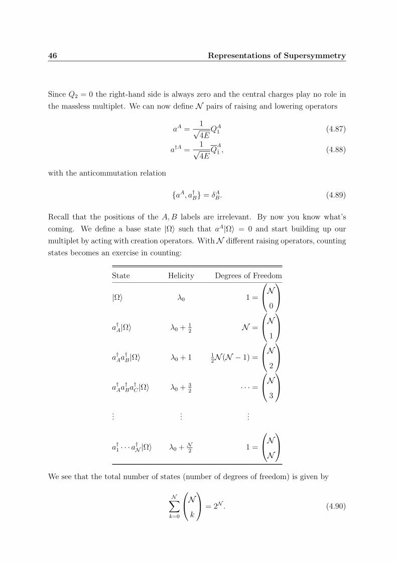
46 Representations of Supersymmetry
Since Q2 = 0 the right-hand side is always zero and the central charges play no role in
the massless multiplet. We can now define N pairs of raising and lowering operators
aA =1√4E
QA1 (4.87)
a†A =1√4E
QA
1 , (4.88)
with the anticommutation relation
aA, a†B = δAB. (4.89)
Recall that the positions of the A,B labels are irrelevant. By now you know what’s
coming. We define a base state |Ω〉 such that aA|Ω〉 = 0 and start building up our
multiplet by acting with creation operators. WithN different raising operators, counting
states becomes an exercise in counting:
State Helicity Degrees of Freedom
|Ω〉 λ0 1 =
N0
a†A|Ω〉 λ0 + 1
2N =
N1
a†Aa
†B|Ω〉 λ0 + 1 1
2N (N − 1) =
N2
a†Aa
†Ba†C |Ω〉 λ0 + 3
2· · · =
N3
...
......
a†1 · · · a†N |Ω〉 λ0 + N
21 =
NN
We see that the total number of states (number of degrees of freedom) is given by
N∑k=0
Nk
= 2N . (4.90)
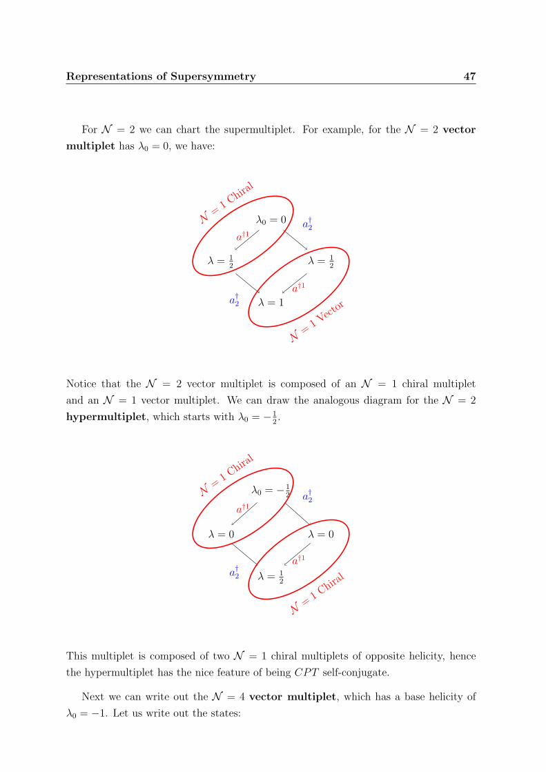
Representations of Supersymmetry 47
For N = 2 we can chart the supermultiplet. For example, for the N = 2 vector
multiplet has λ0 = 0, we have:
λ0 = 0
λ = 1
λ = 12
λ = 12
a†2
a†2
a†1
a†1
N=
1 Chiral
N=
1 Vector
Notice that the N = 2 vector multiplet is composed of an N = 1 chiral multiplet
and an N = 1 vector multiplet. We can draw the analogous diagram for the N = 2
hypermultiplet, which starts with λ0 = −12.
λ0 = −12
λ = 12
λ = 0 λ = 0
a†2
a†2
a†1
a†1
N=
1 Chiral
N=
1 Chiral
This multiplet is composed of two N = 1 chiral multiplets of opposite helicity, hence
the hypermultiplet has the nice feature of being CPT self-conjugate.
Next we can write out the N = 4 vector multiplet, which has a base helicity of
λ0 = −1. Let us write out the states:
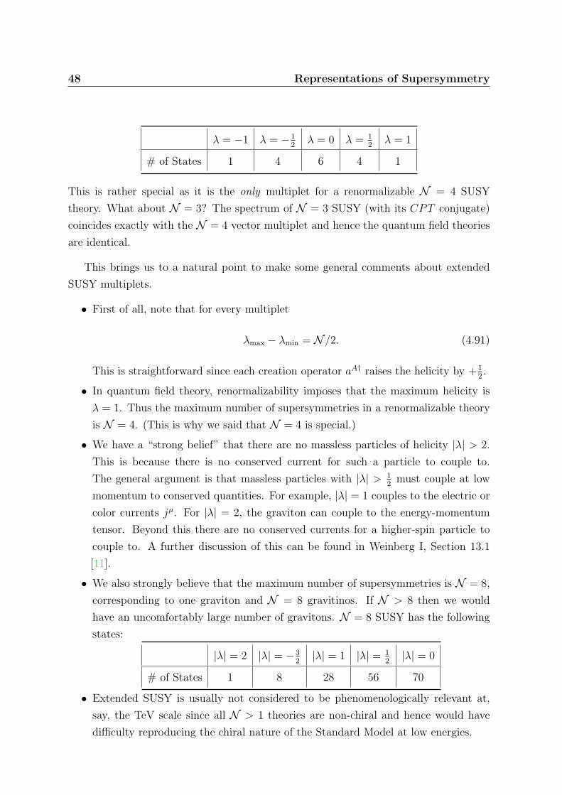
48 Representations of Supersymmetry
λ = −1 λ = −12
λ = 0 λ = 12
λ = 1
# of States 1 4 6 4 1
This is rather special as it is the only multiplet for a renormalizable N = 4 SUSY
theory. What about N = 3? The spectrum of N = 3 SUSY (with its CPT conjugate)
coincides exactly with the N = 4 vector multiplet and hence the quantum field theories
are identical.
This brings us to a natural point to make some general comments about extended
SUSY multiplets.
• First of all, note that for every multiplet
λmax − λmin = N /2. (4.91)
This is straightforward since each creation operator aA† raises the helicity by +12.
• In quantum field theory, renormalizability imposes that the maximum helicity is
λ = 1. Thus the maximum number of supersymmetries in a renormalizable theory
is N = 4. (This is why we said that N = 4 is special.)
• We have a “strong belief” that there are no massless particles of helicity |λ| > 2.
This is because there is no conserved current for such a particle to couple to.
The general argument is that massless particles with |λ| > 12
must couple at low
momentum to conserved quantities. For example, |λ| = 1 couples to the electric or
color currents jµ. For |λ| = 2, the graviton can couple to the energy-momentum
tensor. Beyond this there are no conserved currents for a higher-spin particle to
couple to. A further discussion of this can be found in Weinberg I, Section 13.1
[11].
• We also strongly believe that the maximum number of supersymmetries is N = 8,
corresponding to one graviton and N = 8 gravitinos. If N > 8 then we would
have an uncomfortably large number of gravitons. N = 8 SUSY has the following
states:
|λ| = 2 |λ| = −32|λ| = 1 |λ| = 1
2|λ| = 0
# of States 1 8 28 56 70
• Extended SUSY is usually not considered to be phenomenologically relevant at,
say, the TeV scale since all N > 1 theories are non-chiral and hence would have
difficulty reproducing the chiral nature of the Standard Model at low energies.
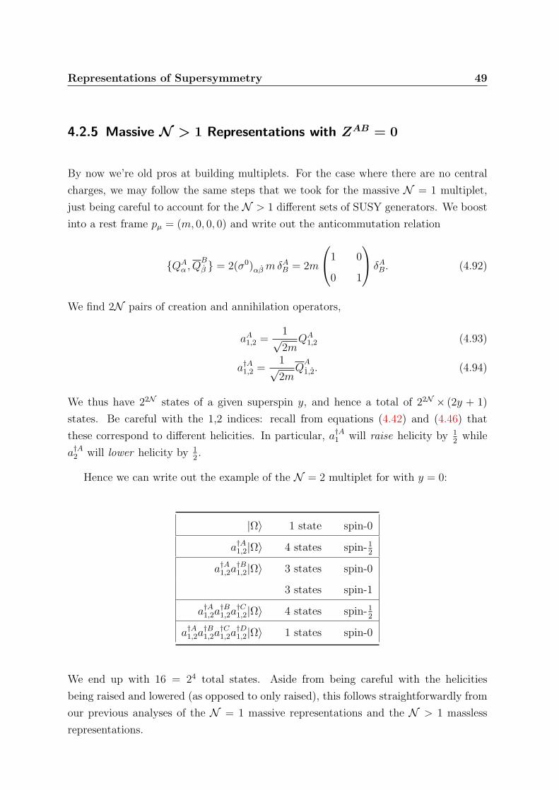
Representations of Supersymmetry 49
4.2.5 Massive N > 1 Representations with ZAB = 0
By now we’re old pros at building multiplets. For the case where there are no central
charges, we may follow the same steps that we took for the massive N = 1 multiplet,
just being careful to account for the N > 1 different sets of SUSY generators. We boost
into a rest frame pµ = (m, 0, 0, 0) and write out the anticommutation relation
QAα , Q
B
β = 2(σ0)αβmδAB = 2m
1 0
0 1
δAB. (4.92)
We find 2N pairs of creation and annihilation operators,
aA1,2 =1√2m
QA1,2 (4.93)
a†A1,2 =1√2m
QA
1,2. (4.94)
We thus have 22N states of a given superspin y, and hence a total of 22N × (2y + 1)
states. Be careful with the 1,2 indices: recall from equations (4.42) and (4.46) that
these correspond to different helicities. In particular, a†A1 will raise helicity by 12
while
a†A2 will lower helicity by 12.
Hence we can write out the example of the N = 2 multiplet for with y = 0:
|Ω〉 1 state spin-0
a†A1,2|Ω〉 4 states spin-12
a†A1,2a†B1,2|Ω〉 3 states spin-0
3 states spin-1
a†A1,2a†B1,2a
†C1,2|Ω〉 4 states spin-1
2
a†A1,2a†B1,2a
†C1,2a
†D1,2|Ω〉 1 states spin-0
We end up with 16 = 24 total states. Aside from being careful with the helicities
being raised and lowered (as opposed to only raised), this follows straightforwardly from
our previous analyses of the N = 1 massive representations and the N > 1 massless
representations.
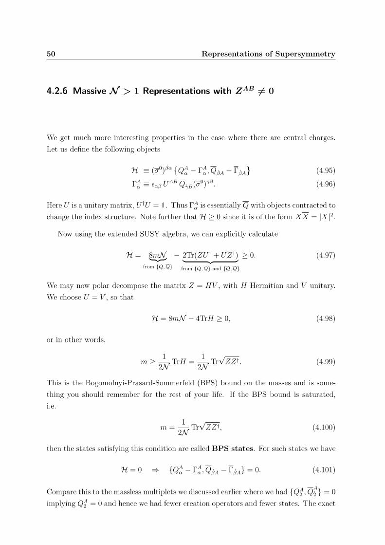
50 Representations of Supersymmetry
4.2.6 Massive N > 1 Representations with ZAB 6= 0
We get much more interesting properties in the case where there are central charges.
Let us define the following objects
H ≡ (σ0)βαQAα − ΓAα , QβA − ΓβA
(4.95)
ΓAα ≡ εαβ UAB QγB(σ0)γβ. (4.96)
Here U is a unitary matrix, U †U = 1. Thus ΓAα is essentially Q with objects contracted to
change the index structure. Note further that H ≥ 0 since it is of the form XX = |X|2.
Now using the extended SUSY algebra, we can explicitly calculate
H = 8mN︸ ︷︷ ︸from Q,Q
− 2Tr(ZU † + UZ†)︸ ︷︷ ︸from Q,Q and Q,Q
≥ 0. (4.97)
We may now polar decompose the matrix Z = HV , with H Hermitian and V unitary.
We choose U = V , so that
H = 8mN − 4TrH ≥ 0, (4.98)
or in other words,
m ≥ 1
2NTrH =
1
2NTr√ZZ†. (4.99)
This is the Bogomolnyi-Prasard-Sommerfeld (BPS) bound on the masses and is some-
thing you should remember for the rest of your life. If the BPS bound is saturated,
i.e.
m =1
2NTr√ZZ†, (4.100)
then the states satisfying this condition are called BPS states. For such states we have
H = 0 ⇒ QAα − ΓAα , QβA − ΓβA = 0. (4.101)
Compare this to the massless multiplets we discussed earlier where we had QA2 , Q
A
2 = 0
implying QA2 = 0 and hence we had fewer creation operators and fewer states. The exact
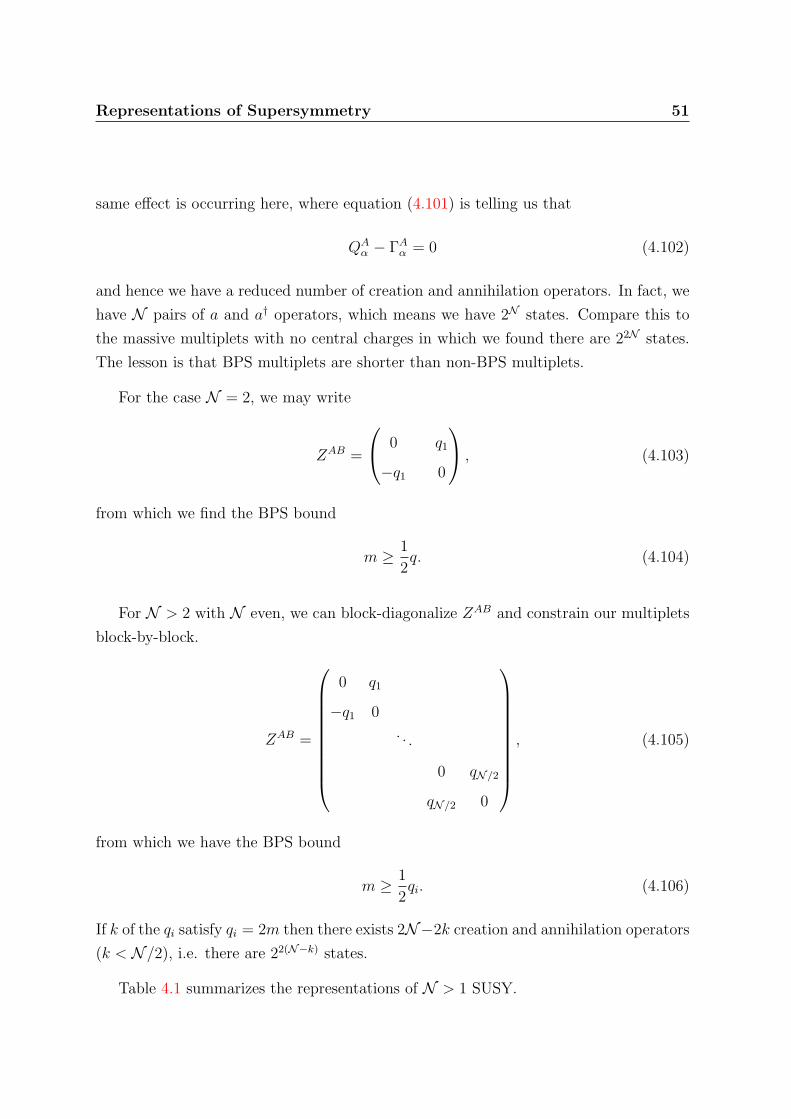
Representations of Supersymmetry 51
same effect is occurring here, where equation (4.101) is telling us that
QAα − ΓAα = 0 (4.102)
and hence we have a reduced number of creation and annihilation operators. In fact, we
have N pairs of a and a† operators, which means we have 2N states. Compare this to
the massive multiplets with no central charges in which we found there are 22N states.
The lesson is that BPS multiplets are shorter than non-BPS multiplets.
For the case N = 2, we may write
ZAB =
0 q1
−q1 0
, (4.103)
from which we find the BPS bound
m ≥ 1
2q. (4.104)
For N > 2 with N even, we can block-diagonalize ZAB and constrain our multiplets
block-by-block.
ZAB =
0 q1
−q1 0
. . .
0 qN/2
qN/2 0
, (4.105)
from which we have the BPS bound
m ≥ 1
2qi. (4.106)
If k of the qi satisfy qi = 2m then there exists 2N−2k creation and annihilation operators
(k < N /2), i.e. there are 22(N−k) states.
Table 4.1 summarizes the representations of N > 1 SUSY.
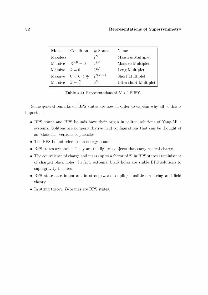
52 Representations of Supersymmetry
Mass Condition # States Name
Massless 2N Massless Multiplet
Massive ZAB = 0 22N Massive Multiplet
Massive k = 0 22N Long Multiplet
Massive 0 < k < N2
22(N−k) Short Multiplet
Massive k = N2
2N Ultra-short Multiplet
Table 4.1: Representations of N > 1 SUSY.
Some general remarks on BPS states are now in order to explain why all of this is
important.
• BPS states and BPS bounds have their origin in soliton solutions of Yang-Mills
systems. Solitons are nonperturbative field configurations that can be thought of
as “classical” versions of particles.
• The BPS bound refers to an energy bound.
• BPS states are stable. They are the lightest objects that carry central charge.
• The equivalence of charge and mass (up to a factor of 2) in BPS states i reminiscent
of charged black holes. In fact, extremal black holes are stable BPS solutions to
supergravity theories.
• BPS states are important in strong/weak coupling dualities in string and field
theory.
• In string theory, D-branes are BPS states.
Chapter 5
Superfields and Superspace
“So in supersymmetry, you have superfields and superpotentials and
everything is ‘super.’ At some point this naming convention becomes
rather ridiculous, doesn’t it? Why not ‘hyper’? I’ll invent my own
theory and call it ‘hypersymmetry;’ then everything will be ‘hyper.’”
— Steffen Gielen, 2007 Mayhew Prize Recipient
So far we’ve been doing purely algebraic manipulations. We know the characters of
the play, but we need a field theory to provide a script describing the dynamics of these
objects. Superspace, developed by Strathdee and Salam in 1974 [12,13], is a convenient
way to do this.
Here we’ll go over the necessary tools for N = 1 (global) superspace. A much more
general and thorough treatment can be found in DeWitt’s text[14] while technical details
for the mathematically-inclined can be found in the notes by Gieres [15]. It is critical to
note that there are no (satisfactory) standard sign and phase conventions in the literature
for the material in this chapter. We will be self-consistent, but it is unlikely that we
will coincide with any other text1. A very useful convention-independent derivation is
presented in Binetruy’s text[17]. We reproduce parts of this derivation in Appendix B.4.
1It’s also unlikely that any two texts will agree. In fact, there are even some texts, e.g. [16], whoseconventions differ for different chapters!
53
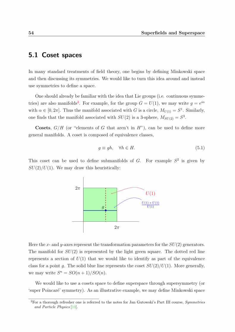
54 Superfields and Superspace
5.1 Coset spaces
In many standard treatments of field theory, one begins by defining Minkowski space
and then discussing its symmetries. We would like to turn this idea around and instead
use symmetries to define a space.
One should already be familiar with the idea that Lie groups (i.e. continuous symme-
tries) are also manifolds2. For example, for the group G = U(1), we may write g = eiα
with α ∈ [0, 2π]. Thus the manifold associated with G is a circle, MU(1) = S1. Similarly,
one finds that the manifold associated with SU(2) is a 3-sphere, MSU(2) = S3.
Cosets, G/H (or “elements of G that aren’t in H”), can be used to define more
general manifolds. A coset is composed of equivalence classes,
g ≡ gh, ∀h ∈ H. (5.1)
This coset can be used to define submanifolds of G. For example S2 is given by
SU(2)/U(1). We may draw this heuristically:
U(1)×U(1)U(1)
U(1)
2π
2π
g
Here the x- and y-axes represent the transformation parameters for the SU(2) generators.
The manifold for SU(2) is represented by the light green square. The dotted red line
represents a section of U(1) that we would like to identify as part of the equivalence
class for a point g. The solid blue line represents the coset SU(2)/U(1). More generally,
we may write Sn = SO(n+ 1)/SO(n).
We would like to use a cosets space to define superspace through supersymmetry (or
‘super Poincare’ symmetry). As an illustrative example, we may define Minkowski space
2For a thorough refresher one is referred to the notes for Jan Gutowski’s Part III course, Symmetriesand Particle Physics [10].
Superfields and Superspace 55
as the coset space ‘Poincare/Lorentz’, or P/SO(3, 1)↑ where P is the Poincare group3.
This is an intuitive statement since one can map the generators of translations with
points on Minkowski space. In slightly more rigor, the generators of the Poincare group
take the form
gP = ei(ωµνMµν+aµPµ), (5.2)
while the generators of the Lorentz group take the form
gL = ei(ωµνMµν). (5.3)
One can thus identify the coset manifold with the translation parameters,
MPoincare/Lorentz = aµ. (5.4)
Multiplication of group elements correspond to successive translations on the Minkowski
manifold. This is, of course, a bit of overkill for the rather trivial case of Minkowski
space.
We now generalize this idea to an (arguably) non-trivial case: the coset space (N =
1 super-Poincare)/Lorentz, or SP/SO(3, 1)↑. We call the resulting manifold N = 1
superspace. The generators of the super-Poincare group take the form
gSP = ei(ωµνMµν+aµPµ+θαQα+θαQ
α), (5.5)
were ωµν and aµ are the usual c-number4 parameters for the Poincare group while θ and
θ are anticommuting Grassmann parameters. Thus we may write coordinates for N = 1
superspace as
aµ, θα, θα. (5.6)
In this sense, supersymmetry is a kind of fermionic extra dimension. The products θQ
and θQ are commuting objects, and so we may write the SUSY algebra using commu-
tators,
Qα, Qα = 2(σµ)ααPµ ⇒ [θαQα, θβQβ] = 2θα(σµ)αβθ
βPµ. (5.7)
3We form the coset using the part of the Lorentz group connected to the identity since this is the partof the Lorentz group included in Poincare symmetry.
4Short for ‘commuting’ number.
56 Superfields and Superspace
This will allow us to apply useful results from non-graded Lie algebras, such as the
Baker-Campbell-Hausdorff formula for the product of exponentiated generators.
Minkowski space and superspace as a coset. For those who would prefer a
slightly more rigorous treatment, one may follow the argument of Section 2.4.1 of
Buchbinder and Kuzenko [3]. An even more formal mathematical treatment can be
found in the first chapter of [15].
Armed with this spacetime extended by Grassmann coordinates, we may proceed to
define superfields as a generalization of the usual fields that live on Minkowski space.
We will see in Section 5.3 that these fields contain entire SUSY multiplets of component
Minkowski-space fields. This will be the ‘punchline’ of what may presently seem like
excessive formalism.
5.2 The Calculus of Grassmann Numbers
Now that we’ve generalized Minkowski space to superspace, we would like to write
Lagrangian densities on superspace such that the action is given by an integration over
d4x d2θ d2θ. In order to do this we’ll have to familiarize ourselves with the calculus of
Grassmann variables. For further references, see DeWitt [14] and Gie.
5.2.1 Scalar Grassmann Variable
We may expand a function of a single Grassmann variable, θ, by Taylor expanding,
f(θ) = f0 + f1θ + f2θ2 + · · · . (5.8)
By the antisymmetry of θ, the f2 term and all higher terms vanish. Hence the most
general function of a single Grassmann variable can be written as
f(θ) = f0 + f1θ. (5.9)
Superfields and Superspace 57
We now define calculus for Grassmann variables. With the expansion above, we can
define differentiation with respect to θ in the natural way,
df
dθ= f1. (5.10)
It is trickier to define integration over Grassmann variables. The integration operator
on superspace is called the Berezin integral. To motivate this integration, we note
that integration over R is translation invariant,∫ ∞−∞
dx f(x) =
∫ ∞−∞
dx f(x+ a). (5.11)
We would like to carry over this sense of translation-invariance for our dθ integral,∫dθ f(θ) =
∫dθ f(θ + α). (5.12)
Using the expansion of equation (5.9), this translates to∫dθ f0 + f1θ =
∫dθ f0 + f1θ + f1α, (5.13)
from which we conclude ∫dθ, f1α = 0. (5.14)
Thus we define the integrals∫dθ = 0
∫dθ θ = 1. (5.15)
If you want you can interpret the first equation to mean that the space spanned by θ
has no boundary, while the second equation is an arbitrary normalization condition that
we choose to be non-zero so that integration is a non-trivial operation. Thus we may
summarize the Berezin integral by the rule∫dθ f(θ) =
∫dθ (f0 + f1θ) = f1 =
df
dθ. (5.16)
We see that derivatives and integrals of Grassmann variables are equivalent.
58 Superfields and Superspace
5.2.2 Spinor Grassmann Variables
Superspace extends Minkowski space with two spinor degrees of freedom, θα and θα, so
we ought to establish conventions for the calculus of Weyl spinor variables. We shall
follow our previously defined convention for the contraction of left- and right-handed
spinor coordinates,
θθ ≡ θαθα θθ ≡ θαθα. (5.17)
Antisymmetry allows us to write out products of spinor components in terms of the
antisymmetric tensor times the spinor contractions as follows,
θαθβ = −1
2εαβθθ θαθβ = −1
2εαβθθ. (5.18)
As before we may define differentiation in the usual way,
∂
∂θαθβ = δβα
∂
∂θαθβ = δβα. (5.19)
Note that ∂/∂θα transforms as a lower-index left-handed spinor (i.e. ψα-type) and ∂/∂θα
transforms as an upper-index right-handed spinor (i.e. χα-type). This is completely
analogous to the case of vector derivatives where ∂/∂xµ transforms as a lower-index
object. Following the convention of equation (5.19), however, we run into an immediate
issue of consistency that requires some care. Suppose we naively defined the ∂/∂θα and
∂/∂θα
partial derivatives in the same way. Then we’d run into problems since (ignoring
the index height on the Kronecker δ),
∂
∂θαθβ = δβα
?=
∂
∂θαθβ, (5.20)
while we also have, from equation (2.59),
∂
∂θαθβ = − ∂
∂θαθβ. (5.21)
The only way for equations (5.20) and (5.21) to be consistent is if both types of deriva-
tives are identically zero. Thus we are led to the following definitions for the lower/upper-
Superfields and Superspace 59
index spinor derivatives,
∂
∂θα= −εαβ ∂
∂θβ∂
∂θα
= −εαβ∂
∂θβ. (5.22)
For consistency we must also define the complex conjugate relations(∂
∂θα
)∗= − ∂
∂θα
(∂
∂θα
)∗= − ∂
∂θα(5.23)
We define the two-dimensional integral as follows,∫d2θ ≡ 1
2
∫dθ1 dθ2, (5.24)
where the factor of 12
comes from writing out
1 =
∫dθ1dθ2 θ2θ1 =
1
2
∫dθ1dθ2 θθ, (5.25)
and thus with this normalization we have∫d2θ (θθ) = 1. (5.26)
We use the same normalization for the right-handed superspace coordinates, and can
thus write the integral over both θ and θ as∫d2θ
∫d2θ (θθ)(θθ) =
∫d4θ (θθ)(θθ) = 1, (5.27)
where we have defined measure d4θ = d2θ d2θ.
It is, perhaps, worth emphasizing that the factor of 12
above is a normalization con-
dition on the Grassmann measure, and not some application of equations (5.18). If one
wanted to use those expressions on the measure, then one could write
d2θ = −1
4dθαdθβεαβ d2θ =
1
4dθ
αdθ
βεαβ. (5.28)
60 Superfields and Superspace
The equivalence of the Berezin integral and the Grassmann derivative can be cast in the
form ∫d2θ =
1
4εαβ
∂
∂θα∂
∂θβ
∫d2θ = −1
4εαβ
∂
∂θα
∂
∂θβ. (5.29)
This will be rather useful as it will allow us to write out particular terms in the Taylor
expansion of a function on superspace by performing superspace integrals.
Finally, we can introduce an inner product for superfields,
〈F (x, θ, θ) , G(x, θ, θ)〉 =
∫d4x d4θ F ∗(x, θ, θ)G(x, θ, θ). (5.30)
This means that we can also define a superspace Hermitian conjugation operation, †.
For example, using integration by parts the Hermitian conjugate of the (Minkowski)
spacetime derivative behaves as
∂ †µ = −∂µ. (5.31)
This Hermitian conjugation is antilinear (i.e. it “represents an involutive anti-homomorphism”),
for complex coefficients a, b and superfields φ, ψ,
(aφ+ bψ)† = φ†a∗ + ψ†b∗ (5.32)
(φψ)† = ψ†φ†. (5.33)
At this point I really have to apologize. I made a big deal on page 15 about stars
and daggers being essentially the same thing: classical fields could get starred (com-
plex conjugated) while quantum fields, being composed of operators, could get daggered
(Hermitian conjugated). I tried to express that different books use different notation,
but that we could afford to be nonchalant about this. Unfortunately, we’ve now defined
yet another kind of dagger that is very different from the star. Note that the superspace
Hermitian conjugation is defined with respect to the superspace inner product of (clas-
sical) superfields and is completely different from the Hermitian conjugation associated
with quantum operators. If one wanted to one could write them separately as † and ‡,
though this introduces a lot of clutter. Fortunately, we will use this superspace Her-
mitian conjugate in Section 5.3 and after that we can forget all of these little technical
details.
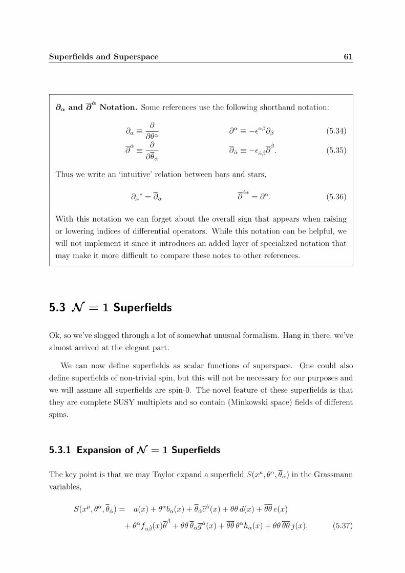
Superfields and Superspace 61
∂α and ∂α
Notation. Some references use the following shorthand notation:
∂α ≡∂
∂θα∂α ≡ −εαβ∂β (5.34)
∂α ≡ ∂
∂θα∂α ≡ −εαβ∂
β. (5.35)
Thus we write an ‘intuitive’ relation between bars and stars,
∂ ∗α = ∂α ∂α∗
= ∂α. (5.36)
With this notation we can forget about the overall sign that appears when raising
or lowering indices of differential operators. While this notation can be helpful, we
will not implement it since it introduces an added layer of specialized notation that
may make it more difficult to compare these notes to other references.
5.3 N = 1 Superfields
Ok, so we’ve slogged through a lot of somewhat unusual formalism. Hang in there, we’ve
almost arrived at the elegant part.
We can now define superfields as scalar functions of superspace. One could also
define superfields of non-trivial spin, but this will not be necessary for our purposes and
we will assume all superfields are spin-0. The novel feature of these superfields is that
they are complete SUSY multiplets and so contain (Minkowski space) fields of different
spins.
5.3.1 Expansion of N = 1 Superfields
The key point is that we may Taylor expand a superfield S(xµ, θα, θα) in the Grassmann
variables,
S(xµ, θα, θα) = a(x) + θαbα(x) + θαcα(x) + θθ d(x) + θθ e(x)
+ θαfαβ(x)θβ
+ θθ θαgα(x) + θθ θαhα(x) + θθ θθ j(x). (5.37)
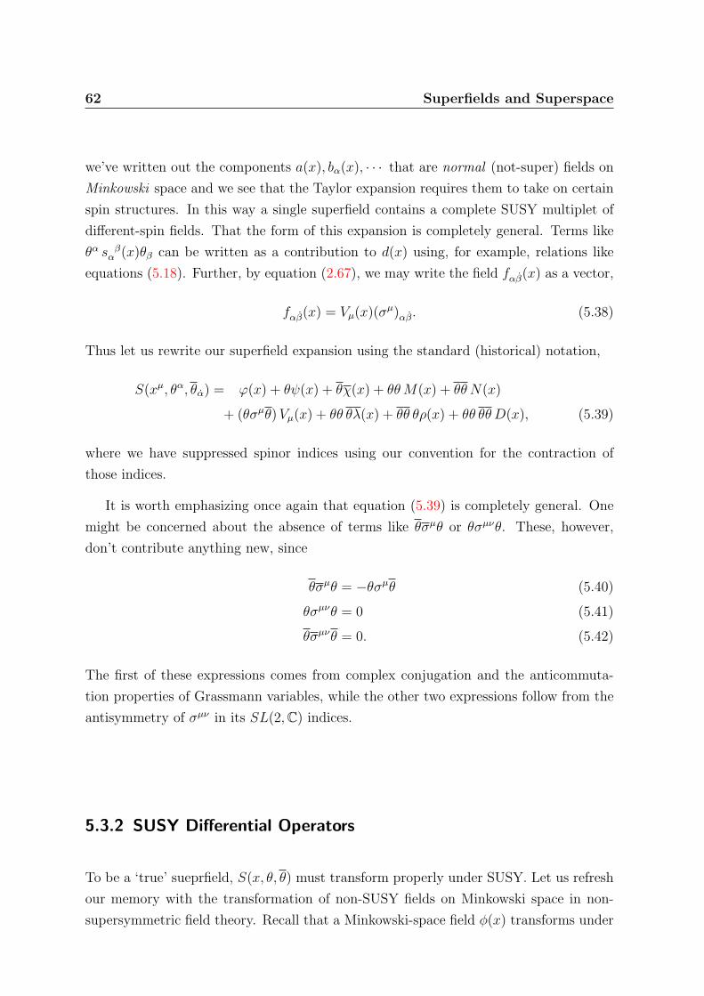
62 Superfields and Superspace
we’ve written out the components a(x), bα(x), · · · that are normal (not-super) fields on
Minkowski space and we see that the Taylor expansion requires them to take on certain
spin structures. In this way a single superfield contains a complete SUSY multiplet of
different-spin fields. That the form of this expansion is completely general. Terms like
θα s βα (x)θβ can be written as a contribution to d(x) using, for example, relations like
equations (5.18). Further, by equation (2.67), we may write the field fαβ(x) as a vector,
fαβ(x) = Vµ(x)(σµ)αβ. (5.38)
Thus let us rewrite our superfield expansion using the standard (historical) notation,
S(xµ, θα, θα) = ϕ(x) + θψ(x) + θχ(x) + θθM(x) + θθ N(x)
+ (θσµθ)Vµ(x) + θθ θλ(x) + θθ θρ(x) + θθ θθ D(x), (5.39)
where we have suppressed spinor indices using our convention for the contraction of
those indices.
It is worth emphasizing once again that equation (5.39) is completely general. One
might be concerned about the absence of terms like θσµθ or θσµνθ. These, however,
don’t contribute anything new, since
θσµθ = −θσµθ (5.40)
θσµνθ = 0 (5.41)
θσµνθ = 0. (5.42)
The first of these expressions comes from complex conjugation and the anticommuta-
tion properties of Grassmann variables, while the other two expressions follow from the
antisymmetry of σµν in its SL(2,C) indices.
5.3.2 SUSY Differential Operators
To be a ‘true’ sueprfield, S(x, θ, θ) must transform properly under SUSY. Let us refresh
our memory with the transformation of non-SUSY fields on Minkowski space in non-
supersymmetric field theory. Recall that a Minkowski-space field φ(x) transforms under
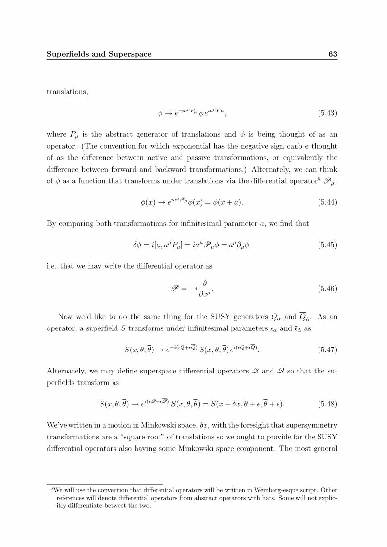
Superfields and Superspace 63
translations,
φ→ e−iaµPµ φ eia
µPµ, (5.43)
where Pµ is the abstract generator of translations and φ is being thought of as an
operator. (The convention for which exponential has the negative sign canb e thought
of as the difference between active and passive transformations, or equivalently the
difference between forward and backward transformations.) Alternately, we can think
of φ as a function that transforms under translations via the differential operator5 Pµ,
φ(x)→ eiaµPµφ(x) = φ(x+ a). (5.44)
By comparing both transformations for infinitesimal parameter a, we find that
δφ = i[φ, aµPµ] = iaµPµφ = aµ∂µφ, (5.45)
i.e. that we may write the differential operator as
P = −i ∂∂xµ
. (5.46)
Now we’d like to do the same thing for the SUSY generators Qα and Qα. As an
operator, a superfield S transforms under infinitesimal parameters εα and εα as
S(x, θ, θ)→ e−i(εQ+εQ) S(x, θ, θ) ei(εQ+εQ). (5.47)
Alternately, we may define superspace differential operators Q and Q so that the su-
perfields transform as
S(x, θ, θ)→ ei(εQ+εQ) S(x, θ, θ) = S(x+ δx, θ + ε, θ + ε). (5.48)
We’ve written in a motion in Minkowski space, δx, with the foresight that supersymmetry
transformations are a “square root” of translations so we ought to provide for the SUSY
differential operators also having some Minkowski space component. The most general
5We will use the convention that differential operators will be written in Weinberg-esque script. Otherreferences will denote differential operators from abstract operators with hats. Some will not explic-itly differentiate betweet the two.
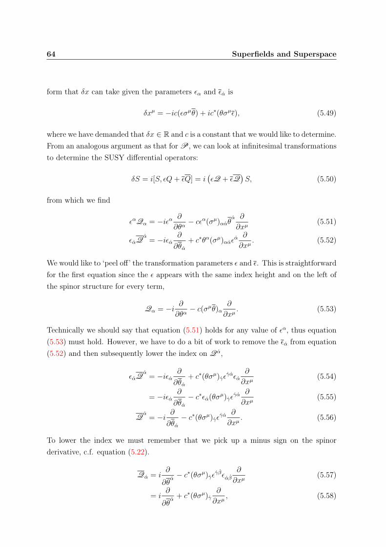
64 Superfields and Superspace
form that δx can take given the parameters εα and εα is
δxµ = −ic(εσµθ) + ic∗(θσµε), (5.49)
where we have demanded that δx ∈ R and c is a constant that we would like to determine.
From an analogous argument as that for P, we can look at infinitesimal transformations
to determine the SUSY differential operators:
δS = i[S, εQ+ εQ] = i(εQ + εQ
)S, (5.50)
from which we find
εαQα = −iεα ∂
∂θα− cεα(σµ)ααθ
α ∂
∂xµ(5.51)
εαQα
= −iεα∂
∂θα+ c∗θα(σµ)ααε
α ∂
∂xµ. (5.52)
We would like to ‘peel off’ the transformation parameters ε and ε. This is straightforward
for the first equation since the ε appears with the same index height and on the left of
the spinor structure for every term,
Qα = −i ∂∂θα− c(σµθ)α
∂
∂xµ. (5.53)
Technically we should say that equation (5.51) holds for any value of εα, thus equation
(5.53) must hold. However, we have to do a bit of work to remove the εα from equation
(5.52) and then subsequently lower the index on Qα,
εαQα
= −iεα∂
∂θα+ c∗(θσµ)γε
γαεα∂
∂xµ(5.54)
= −iεα∂
∂θα− c∗εα(θσµ)γε
γα ∂
∂xµ(5.55)
Qα
= −i ∂∂θα− c∗(θσµ)γε
γα ∂
∂xµ. (5.56)
To lower the index we must remember that we pick up a minus sign on the spinor
derivative, c.f. equation (5.22).
Qα = i∂
∂θα− c∗(θσµ)γε
γβεαβ∂
∂xµ(5.57)
= i∂
∂θα
+ c∗(θσµ)γ∂
∂xµ, (5.58)
Superfields and Superspace 65
where we’ve used εαβεβγ = δγα. In order to satisfy the SUSY anticommutation relation
Qα,Q β = 2(σµ)αβ = Pµ, one must have <e c = 1. We shall choose c = 1. In
summary, the differential operators associated with our SUSY generators are given by,
P = −i ∂∂xµ
(5.59)
Qα = −i ∂∂θα− (σµθ)α
∂
∂xµ(5.60)
Qα = i∂
∂θα
+ (θσµ)α∂
∂xµ(5.61)
5.3.3 Differential Operators as a Motion in Superspace
There is an alternate way of viewing these differential operators in terms of a motion on
the coset space Poincare/Lorentz6. We may exponentiate the SUSY algebra (a graded
Lie algebra) using the translation parameter a and the SUSY Grassmann parameters ε,
ε, yielding a Lie group element
G(x, θ, θ) = ei(±xµPµ+θQ+θQ), (5.62)
where we have written the translation with a ‘± ’ to indicate some arbitrariness in the
convention for how we define the translation operator (FLIP ***: I don’t think it’ll
matter in the end. Also has to do with active vs passive transformations. Further, the
choice of sign DEFINES what we mean by a forward translation. I SHOULD review
the translation case?) Because the product of two Grassmann variables (e.g. θQ) is a
commuting object, we may apply the Baker-Campbell-Hausdorff formula to products of
group elements,
eA eB = eA+B+ 12
[A,B]+···. (5.63)
Thus we find,
G(0, ε, ε)G(xµ, θ, θ) = ei(εQ+εQ)+i(±xµPµ+θQ+θQ)− 12
[εQ+εQ , ±xµPµ+θQ+θQ]. (5.64)
6This is the approach used in standard texts like Wess & Bagger and Bailin & Love. While the generalprocedure is identical, note that these two references differ from us and from each other by minussigns and factors of i.
66 Superfields and Superspace
We’d like to work out the commutator using the SUSY algebra of equations (3.3) - (3.9).
[εQ+ εQ , ±xµPµ + θQ+ θQ] = [εQ, θQ] + [εQ, θQ]. (5.65)
Since it can be illustrative to work out the arithmetic explicitly at least once in one’s
life, let’s do the first commutator on the right-hand side. One just has to be careful with
anticommuting the Grassmann numbers.
[εQ, θQ] = εαQαθβQβ − θβQ
βεαQα (5.66)
= −εαθβQαQβ
+ θβεαQ
βQα (5.67)
= −εαθβQαQβ − εαθβQ
βQα (5.68)
= −εαθβ [Qα, Qβ] (5.69)
= −εαθβ 2(σµ) βα Pµ (5.70)
= −2(εσµθ)Pµ. (5.71)
Note that the last line doesn’t introduce an overall sign since (σµ) βα = (σµ)αγε
γβ is a
matrix of commuting numbers. Doing the same manipulation for the second commutator
in equation (5.65), we may thus write equation (5.64) as
G(0, ε, ε)G(xµ, θ, θ) = ei[±xµPµ+(ε+θ)Q+(ε+θ)Q]− 1
2[2(εσµθ)Pµ−2(θσµε)Pµ] (5.72)
= ei[(±xµ−iεσµθ+iθσµε)Pµ+(ε+θ)Q+(ε+θ)Q] (5.73)
= G(x∓ iεσµθ± iθσµε , (ε+ θ) , (ε+ θ)). (5.74)
Notice that the ± and ∓ signs have moved to the SUSY-generated Minkowski transla-
tions. This is simply a statement of our convention for a forward spacetime translation.
Thus we may associate the left-multiplication of group elements as a motion in the
parameter space (which is identified with superspace),
g(ε, ε) : (xµ, θ, θ)→ (xµ∓ iεσµθ± iθσµε , (θ + ε) , (θ + ε)). (5.75)
We may thus write out a representation of differential operators for the SUSY generators
following the ‘template’ of equation (5.44),
eiaµPµ+iεQ+iεQS(x, θ, θ) = S(xµ∓ iεσµθ± iθσµε , (θ + ε) , (θ + ε)), (5.76)
Superfields and Superspace 67
so that (keeping particular care with factors of i and signs):
εαQα = −iεα ∂
∂θα∓ iεα(σµ)αβθ
βPµ (5.77)
= −iεα ∂
∂θα∓ iεα(σµ)αβθ
β(∓ i∂µ) (5.78)
= −iεα ∂
∂θα− εα(σµ)αβθ
β∂µ. (5.79)
Note that the dependence on our ‘± ’ convention has dropped out. We can then ‘peel
off’ the εα to find the differential operator
Qα = −i ∂∂θα− (σµ)αβθ
β∂µ. (5.80)
We may now do the same manipulation for the εQ term,
εαQα
= −iεα∂
∂θα± iθβ(σµ)βαε
αPµ (5.81)
= −iεα∂
∂θα± iθβ(σµ)βαε
α(∓ i∂µ) (5.82)
= −iεα∂
∂θα+ θβ(σµ)βαε
α(∂µ). (5.83)
This requires a bit more care to peel off the εα. We will make use of the relations in
equation (2.60) to swap the order of a spinor contraction
εαQα
= −iεα∂
∂θα+ θβ(σµ)βαε
α(∂µ). (5.84)
These match equations (5.51) and (5.52) that we derived using the operator/field ap-
proach.
ACK... my signs are wrong all over the place. I should just work it all out myself
and see what happens. GRARGHRGH. This is a total mess. See Aitchison, sec 6.1;
Binetruy, app C. I think Aitchison 6.1 p. 94 is the most useful.
We have to pcik a representation for P.
• QUEVEDO: e−iaPφeiaP , P = −i∂, exp(θQ+ θQ− xP )
• AITCHISON: eiaPφe−iaP , P = i∂, exp(θQ+ θQ+ xP )
• BAILIN LOVE: eiaPφe−iaP , P =? neg sign?,exp(θQ+ θQ− xP )
• WESS BAGGER: e−iaPφeiaP , P = −i∂, exp(θQ+ θQ− xP )
68 Superfields and Superspace
• BINETRUY: eiaPφe−iaP , P = i∂, exp(θQ+ θQ+ xP )
I should make a table of this in the back. Also, I should follow the argument of
Aitchison.

Chapter 6
SUSY Breaking
“Supersymmetry is elegant, beautiful, and broken.”
— Fernando Quevedo
...
6.1 ...
2-1 relationship
69

70
Chapter 7
XD Basics
“Insert quote.”
— Quote [2]
7.1 Notation and conventions used in this document
XD Basics
7.2 Notes
... for “orbifold or interval” discussion, see Csaba/Jay/Patrick’s notes.
71

72
Chapter 8
Philosophy of Extra Dimensions
“I need to change the title.”
— Fill this in
Here we’d like to talk about XD as an effective field theory. Also perhaps motivate
study of RS through Strong Coupling. See [18].
8.1 5D as EFT
5D Theory is nonrenormalizable, thus it only makes sense as an EFT. That’s fine. The
more religous among us can wave our hands and point to string theory at some high
scale. However, there are things that we can calculate that are manifestly finite, these
are real predictions.
8.2 RS and Holography
Now perhaps a more phenomenologically appealing reason why warped extra dimensions
is interesting is as a playground for the AdS/CFT duality. This way we can use RS to
study strong coupling.
73

74
Chapter 9
Propagators in Extra Dimensions
“Fill this in with a real quote.”
— Fill this in
It is instructive to go over XD propagators. We’ll introduce them in mixed position-
/momentum-space. See [18].
9.1 Propagators on R5
9.1.1 Scalar Propagator
L =1
2∂Aφ∂
Aφ− 1
2m2φ2
=1
2∂µφ∂
µφ− 1
2(∂5φ)2 − 1
2m2φ2
(− + (∂5)2 −m2
)φ = 0 (9.1)
Recall that the propagator is just the Green’s function of this operator,
75
76 Propagators in Extra Dimensions
(− + (∂5)2 −m2
)SF (x− x′, y, y′) = iδ(d−1)(x− x′)δ(y − y′)
We already know the solution to this equation
SF (x− x′, y, y′) =
∫ddp
(2π)2
i
p2 − (p5)2 −m2 + iεe−i(p · (x−x′)−p5(y−y′)) (9.2)
9.1.2 Fermion Propagator
This is nontrivial? (iΓA∂A −m)ψ = 0.
∂5 −m iσµ∂µ
iσµ∂µ −∂5 −m
ψ = 0. (9.3)
Using Dirac representation used in Peskin & Schroeder.
9.1.3 Gauge boson propagator
9.2 Propagators on R4×S1
Let’s now compactify the fifth dimension on S1. Let us begin with a bit of a digression.
There is a very interesting relation between statistical physics and quantum field theory
that one can see just from looking at the partition function. (See Zee) The heart of
the matter is that there is a relation between the inverse temperature β and the Planck
constant ~. Here’s the beautiful thing that comes from this relation: when one wants
to do finite temperature field theory, one simply does a wick rotation to impose periodic
boundary conditions on the Euclidean time. Of course in the Euclidean theory one
can’t really tell space and time apart, so we may borrow from the framework of finite
temperature field theory to work with a compactified (i.e. periodic boundary conditions)
spatial dimension. Good reference: Kasputin.
Propagators in Extra Dimensions 77
We will write the 4D momentum as pµ. If pµ5D is the 5D momentum, then
p25D = m2
= p2 − n2
R2.
Thus it will be useful to write
p2 = m2 +n2
R2. (9.4)
9.2.1 Scalar Propagator
For the scalar propagator we can be a bit more general and work with d − 1 infinite
spacetime dimensions with on dimension compactified on S1. We shall take a hint from
finite temperature field theory and write our compactified-space propagator ScF as an
infinite sum of uncompactified propagators from equation (9.2):
ScF (x− x′, y, y′) =∞∑
n=−∞
SF (x− x′, y + 2πRn, y′). (9.5)
This, by construction, satisfies the periodic boundary conditions imposed by the
compactification. More intuitively, the propagator represents the summing of all paths
between two points weighted by the exponential of the action. Thus in equation (9.5)
we are pretending that the space is not compact but that instead of just summing over
all paths between the initial point and the class of points that are identified by the
compactification. This is shown heuristically in Figure 9.1... though here I’ve added the
2πRn to the end point not the initial point. I should fix this. Really what we’re doing
is a sum over n winding modes around the compact dimension.
One can go ahead and compute the p5 integral explicitly and writing χ =√p2 −m2 + iε,
ScF (x− x′, y, y′) =∞∑
n=−∞
∫dd−1p
(2π)d−1
∫dp5
2π
ie−i(p · (x−x′)−p5(y+2πRny′))
p2 − (p5)2 −m2 + iε
=∞∑
n=−∞
∫dd−1p
(2π)d−1
eiχ|y−y′+2πRn|
2χe−ip · (x−x′).
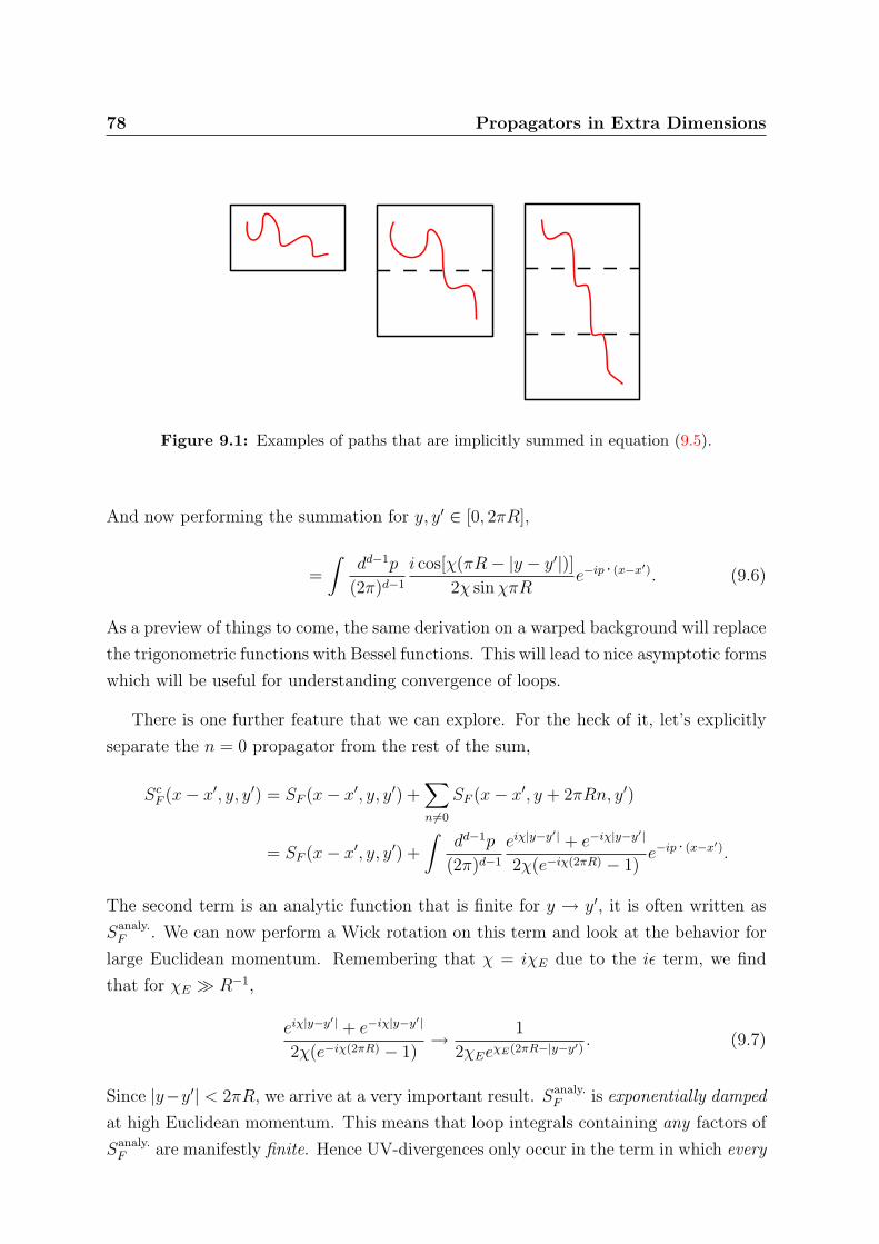
78 Propagators in Extra Dimensions
Figure 9.1: Examples of paths that are implicitly summed in equation (9.5).
And now performing the summation for y, y′ ∈ [0, 2πR],
=
∫dd−1p
(2π)d−1
i cos[χ(πR− |y − y′|)]2χ sinχπR
e−ip · (x−x′). (9.6)
As a preview of things to come, the same derivation on a warped background will replace
the trigonometric functions with Bessel functions. This will lead to nice asymptotic forms
which will be useful for understanding convergence of loops.
There is one further feature that we can explore. For the heck of it, let’s explicitly
separate the n = 0 propagator from the rest of the sum,
ScF (x− x′, y, y′) = SF (x− x′, y, y′) +∑n 6=0
SF (x− x′, y + 2πRn, y′)
= SF (x− x′, y, y′) +
∫dd−1p
(2π)d−1
eiχ|y−y′| + e−iχ|y−y
′|
2χ(e−iχ(2πR) − 1)e−ip · (x−x′).
The second term is an analytic function that is finite for y → y′, it is often written as
Sanaly.F . We can now perform a Wick rotation on this term and look at the behavior for
large Euclidean momentum. Remembering that χ = iχE due to the iε term, we find
that for χE R−1,
eiχ|y−y′| + e−iχ|y−y
′|
2χ(e−iχ(2πR) − 1)→ 1
2χEeχE(2πR−|y−y′) . (9.7)
Since |y−y′| < 2πR, we arrive at a very important result. Sanaly.F is exponentially damped
at high Euclidean momentum. This means that loop integrals containing any factors of
Sanaly.F are manifestly finite. Hence UV-divergences only occur in the term in which every
Propagators in Extra Dimensions 79
loop propagator is SF (x−x′, y, y′). The counterterms of the compact and uncompactified
theories are exactly the same. This makes sense since UV-divergences are short-distance
effects that do not ‘see’ the compactification radius. In thermal language, a T 6= 0 theory
has the exact same divergences as its corresponding T = 0 limit.
As a sanity check, taking R → ∞ (uncompactifying the extra dimension) we find
Sanaly.F → 0 since the winding modes decouple.
9.2.2 Fermion Propagator
At this point, one might guess the mixed position/momentum-space propagator for
fermions. Since any particle obeying the Dirac equation simultaneously obeys the Klein-
Gordon equation, one can expect a factor resembling the Klein-Gordon propagator in
equation (9.6). comparing to the relation of the 4D Dirac and Klein-Gordon propagators,
one could eventually guess that the correct form of the fermion propagator,
ScF (x− x′, y, y′) =
∫d4p
(2π)4
(pµγ
µ + iγ5∂5 +m) i cos[χ(πR− |y − y′|)]
2χ sinχπRe−ip · (x−x′).
(9.8)
We use the same convention as in the scalar case an write χ =√p2 −m2 + iε, with pµ
the 4D momentum. To check that this is correct, one simply needs to plug back into
the 5D Dirac equation, (9.3).
We can derive this equation a bit more formulaically by retracing our derivation
of the 4D Dirac equation while adding some 5D space dependence. We first start by
reconstructing the [‘classical’] plane wave solutions to the Dirac equation, the usual u(p)
and v(p) spinors of 4D QFT.
We start by writing out an explicit positive-energy 4D plane wave expansion, leaving
the y-dependence explicit in the plane wave spinors,
ψ(x, y) = u(p, y)eip ·x. (9.9)
The periodic boundary conditions of S1 imply that these 4D plane waves must depend
on the compactified dimension as a superposition of sin(ny/R) and cos(ny/R). For the
80 Propagators in Extra Dimensions
case n = 0 we should recover the usual 4D plane wave spinor,
u+s,0(p, y) =
√p ·σξs√p ·σξs
. (9.10)
Here ξ is a normalized Weyl 2-spinor such that ξs†ξr = δsr. The index s indicates
the spinor index, the 0 refers to the mode number in the periodic direction, and the
‘+’ superscript indicates that we’re looking at the cos solutions of the periodic bound-
ary conditions–we’ll get to on this in a bit. More generally, we can write down the y
dependence right into the plane waves:
us,n(p, y) =
(A cos(ny/R) +B sin(ny/R))√p ·σξs
(C cos(ny/R) +D sin(ny/R))√p ·σξs
. (9.11)
This explicitly satisfies our boundary conditions in the y-direction. We fix the coefficients
by requiring that u(p, y) is in the kernel of the Dirac operator of equation (9.3), which we
shall write succinctly as D. It is sufficient to only look at only the upper 2 components.
(Du)ups,n =
(−nrA sin
(nyR
)+n
rB cos
(nyR
)−mA cos
(nyR
)−mB sin
(nyR
))√p ·σξ
+(C cos
(nyR
)+D sin
(nyR
))p ·σ
√p ·σξ. (9.12)
Recall that the ‘√p ·σ’ is really just shorthand notation for the square root of the positive
eigenvalue of the matrix, following the convention of Peskin & Schroeder’s derivation of
the 4D plane waves. Further, recall from equation (9.4) that p ·σ p ·σ = m2, where
m2 = m2 +n2
R2. (9.13)
Collecting the coefficients of the sine and cosine and mandating that they each sum to
zero (hence satisfying the Dirac condition), we find
− nRA−mB +mD = 0 (9.14)
n
RB −mA+mC = 0. (9.15)
These relate the coefficients of the lower Weyl spinor (C,D) to those in the upper Weyl
spinor (A,B). We are free to choose basis spinors with A = 1, B = 0 and A = 0, B = 1.
We shall label the former with a ‘+’ superscript and the latter with a ‘−’ superscript.
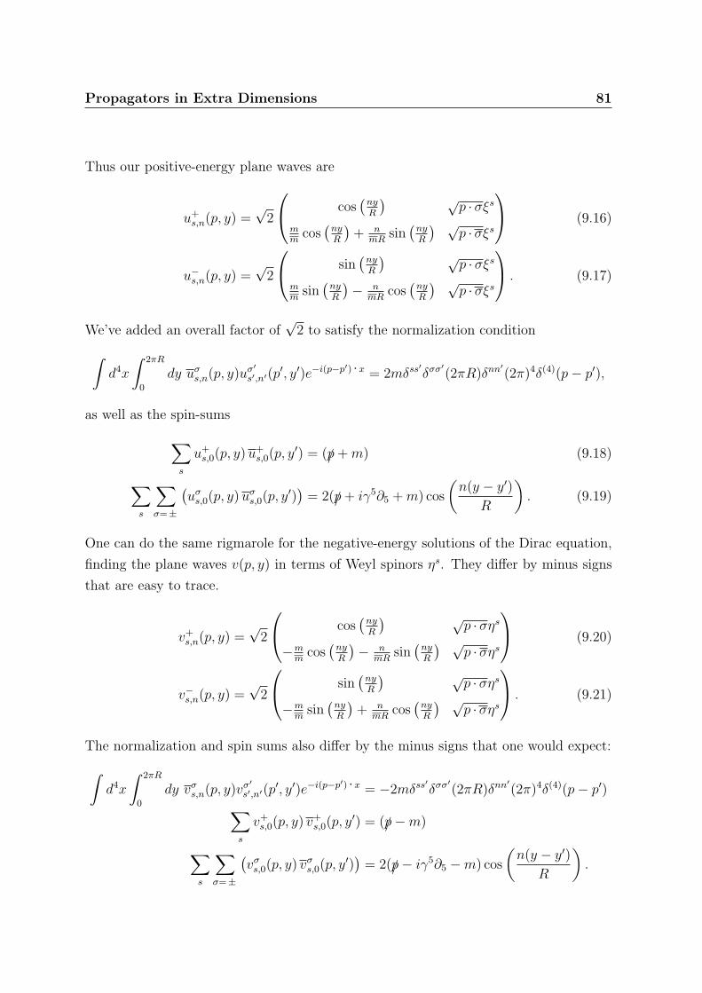
Propagators in Extra Dimensions 81
Thus our positive-energy plane waves are
u+s,n(p, y) =
√2
cos(nyR
) √p ·σξs
mm
cos(nyR
)+ n
mRsin(nyR
) √p ·σξs
(9.16)
u−s,n(p, y) =√
2
sin(nyR
) √p ·σξs
mm
sin(nyR
)− n
mRcos(nyR
) √p ·σξs
. (9.17)
We’ve added an overall factor of√
2 to satisfy the normalization condition∫d4x
∫ 2πR
0
dy uσs,n(p, y)uσ′
s′,n′(p′, y′)e−i(p−p
′) ·x = 2mδss′δσσ
′(2πR)δnn
′(2π)4δ(4)(p− p′),
as well as the spin-sums∑s
u+s,0(p, y)u+
s,0(p, y′) = (/p+m) (9.18)
∑s
∑σ=±
(uσs,0(p, y)uσs,0(p, y′)
)= 2(/p+ iγ5∂5 +m) cos
(n(y − y′)
R
). (9.19)
One can do the same rigmarole for the negative-energy solutions of the Dirac equation,
finding the plane waves v(p, y) in terms of Weyl spinors ηs. They differ by minus signs
that are easy to trace.
v+s,n(p, y) =
√2
cos(nyR
) √p ·σηs
−mm
cos(nyR
)− n
mRsin(nyR
) √p ·σηs
(9.20)
v−s,n(p, y) =√
2
sin(nyR
) √p ·σηs
−mm
sin(nyR
)+ n
mRcos(nyR
) √p ·σηs
. (9.21)
The normalization and spin sums also differ by the minus signs that one would expect:∫d4x
∫ 2πR
0
dy vσs,n(p, y)vσ′
s′,n′(p′, y′)e−i(p−p
′) ·x = −2mδss′δσσ
′(2πR)δnn
′(2π)4δ(4)(p− p′)∑
s
v+s,0(p, y) v+
s,0(p, y′) = (/p−m)
∑s
∑σ=±
(vσs,0(p, y) vσs,0(p, y′)
)= 2(/p− iγ5∂5 −m) cos
(n(y − y′)
R
).
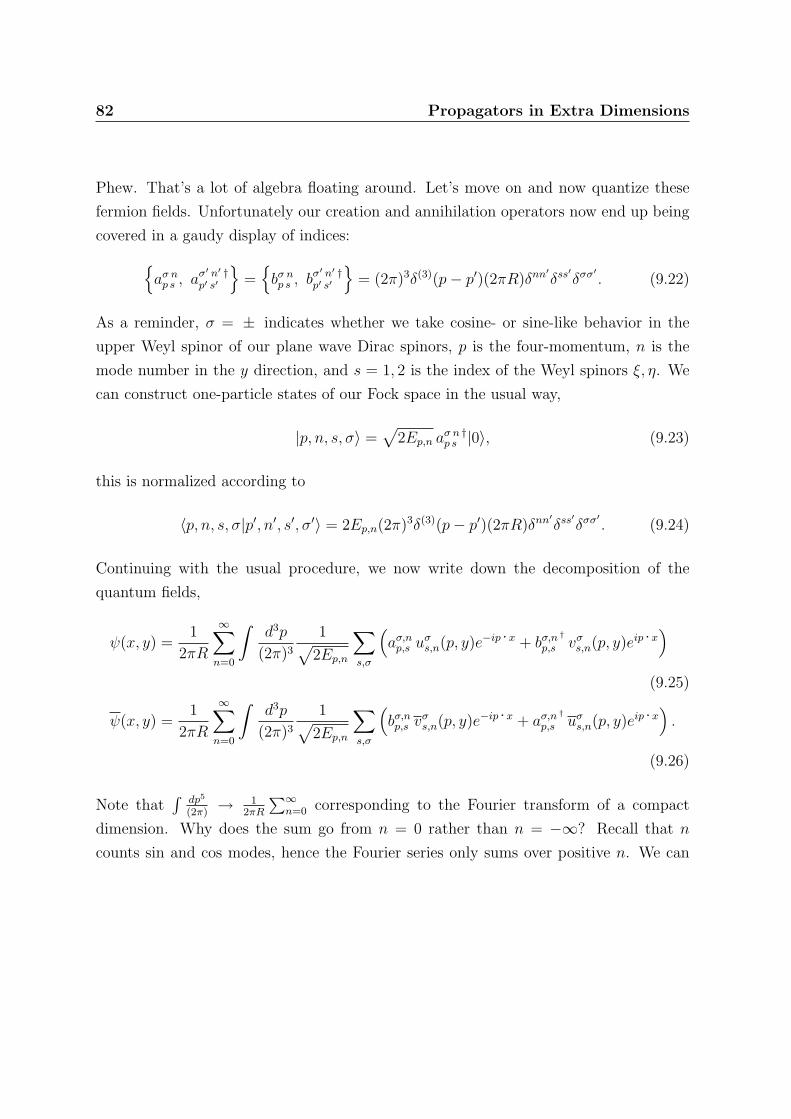
82 Propagators in Extra Dimensions
Phew. That’s a lot of algebra floating around. Let’s move on and now quantize these
fermion fields. Unfortunately our creation and annihilation operators now end up being
covered in a gaudy display of indices:aσ np s , a
σ′ n′ †p′ s′
=bσ np s , b
σ′ n′ †p′ s′
= (2π)3δ(3)(p− p′)(2πR)δnn
′δss
′δσσ
′. (9.22)
As a reminder, σ = ± indicates whether we take cosine- or sine-like behavior in the
upper Weyl spinor of our plane wave Dirac spinors, p is the four-momentum, n is the
mode number in the y direction, and s = 1, 2 is the index of the Weyl spinors ξ, η. We
can construct one-particle states of our Fock space in the usual way,
|p, n, s, σ〉 =√
2Ep,n aσ n †p s |0〉, (9.23)
this is normalized according to
〈p, n, s, σ|p′, n′, s′, σ′〉 = 2Ep,n(2π)3δ(3)(p− p′)(2πR)δnn′δss
′δσσ
′. (9.24)
Continuing with the usual procedure, we now write down the decomposition of the
quantum fields,
ψ(x, y) =1
2πR
∞∑n=0
∫d3p
(2π)3
1√2Ep,n
∑s,σ
(aσ,np,s u
σs,n(p, y)e−ip ·x + bσ,n
†
p,s vσs,n(p, y)eip ·x)
(9.25)
ψ(x, y) =1
2πR
∞∑n=0
∫d3p
(2π)3
1√2Ep,n
∑s,σ
(bσ,np,s v
σs,n(p, y)e−ip ·x + aσ,n
†
p,s uσs,n(p, y)eip ·x).
(9.26)
Note that∫
dp5
(2π)→ 1
2πR
∑∞n=0 corresponding to the Fourier transform of a compact
dimension. Why does the sum go from n = 0 rather than n = −∞? Recall that n
counts sin and cos modes, hence the Fourier series only sums over positive n. We can
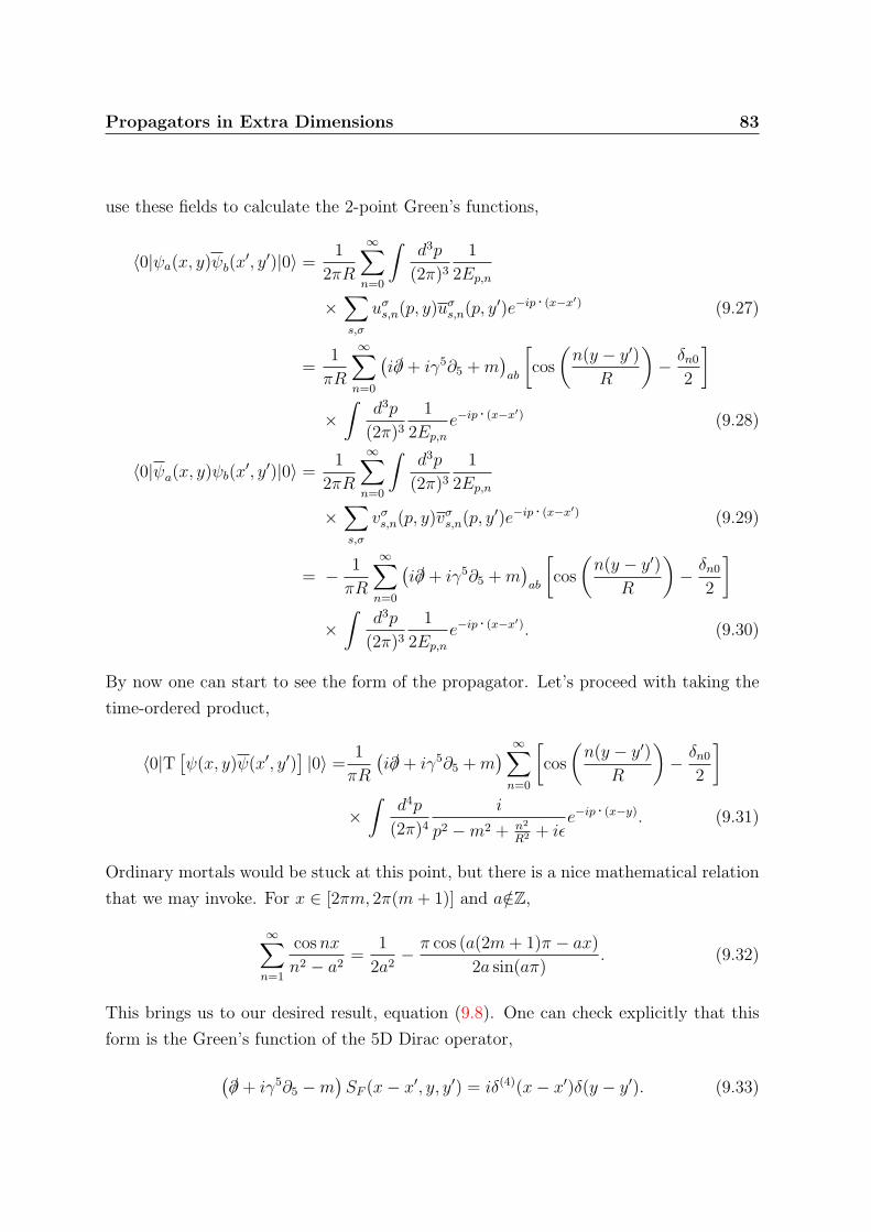
Propagators in Extra Dimensions 83
use these fields to calculate the 2-point Green’s functions,
〈0|ψa(x, y)ψb(x′, y′)|0〉 =
1
2πR
∞∑n=0
∫d3p
(2π)3
1
2Ep,n
×∑s,σ
uσs,n(p, y)uσs,n(p, y′)e−ip · (x−x′) (9.27)
=1
πR
∞∑n=0
(i/∂ + iγ5∂5 +m
)ab
[cos
(n(y − y′)
R
)− δn0
2
]×∫
d3p
(2π)3
1
2Ep,ne−ip · (x−x′) (9.28)
〈0|ψa(x, y)ψb(x′, y′)|0〉 =
1
2πR
∞∑n=0
∫d3p
(2π)3
1
2Ep,n
×∑s,σ
vσs,n(p, y)vσs,n(p, y′)e−ip · (x−x′) (9.29)
= − 1
πR
∞∑n=0
(i/∂ + iγ5∂5 +m
)ab
[cos
(n(y − y′)
R
)− δn0
2
]×∫
d3p
(2π)3
1
2Ep,ne−ip · (x−x′). (9.30)
By now one can start to see the form of the propagator. Let’s proceed with taking the
time-ordered product,
〈0|T[ψ(x, y)ψ(x′, y′)
]|0〉 =
1
πR
(i/∂ + iγ5∂5 +m
) ∞∑n=0
[cos
(n(y − y′)
R
)− δn0
2
]×∫
d4p
(2π)4
i
p2 −m2 + n2
R2 + iεe−ip · (x−y). (9.31)
Ordinary mortals would be stuck at this point, but there is a nice mathematical relation
that we may invoke. For x ∈ [2πm, 2π(m+ 1)] and a/∈Z,
∞∑n=1
cosnx
n2 − a2=
1
2a2− π cos (a(2m+ 1)π − ax)
2a sin(aπ). (9.32)
This brings us to our desired result, equation (9.8). One can check explicitly that this
form is the Green’s function of the 5D Dirac operator,
(/∂ + iγ5∂5 −m
)SF (x− x′, y, y′) = iδ(4)(x− x′)δ(y − y′). (9.33)
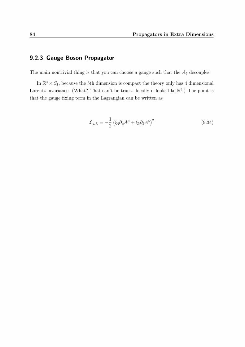
84 Propagators in Extra Dimensions
9.2.3 Gauge Boson Propagator
The main nontrivial thing is that you can choose a gauge such that the A5 decouples.
In R4×S1, because the 5th dimension is compact the theory only has 4 dimensional
Lorentz invariance. (What? That can’t be true... locally it looks like R5.) The point is
that the gauge fixing term in the Lagrangian can be written as
Lg.f. = −1
2
(ξ4∂µA
µ + ξ5∂5A5)2
(9.34)
Appendix A
Literature Guide
“There are more conventions than there are authors.”
— Adrian Signer
...
A.1 General Textbooks
... Aitchison is a relatively new book that is extremely pedagogical. Maybe a little
chatty for those who are already familiar with the topic, but very useful for looking for
a discussion of basic topics. ... Wess and Bagger is the classic with an approach closes
to these notes. Rather technical for reading by itself ... Binetruy has nice appendices,
but strange ordering of topics, Majorana spinors. ... Freund is ... short ... Weinberg
is only comprehensible by Weinberg. But it’s quite good. These notes were (indireclty)
heavily influence by Weinberg. Stupid notation and stupid conventions.
... Drees... sparticles? ... Tata ... Weak scale SUSY? ... Terning ... Modern SUSY
is an advanced book.
... Buchbinder and Kuzenko ... formalism of symmetries
85
86 Literature Guide
A.2 Canonical Reviews
... Stephen Martin. Rather complimentary to our approach, doesn’t use superfields but
instead works directly with component fields to understand physical significance of susy.
Lots of collider stuff. Sign convention may be flipped using tex.
... Argyres. Well written, many versions
A.3 Specialized Reviews
... strassler
A.4 SUSY Breaking
Appendix B
Notation and Conventions
“Insert quote.”
— Quote [2]
B.1 Notation and conventions used in this document
We use the West Coast ‘mostly-minus’ metric that is standard for particle physicists,
η = diag(+,−,−,−). (B.1)
When indices are not important, we shall refer to vector and tensor quantities by writing
them in boldface. Thus we might write M to refer to the tensor Mµν .
SUSY: Greek lowercase letters denote the usual indices in Minkowski space, µ ∈0, 1, 2, 3. Roman lowercase letters around i denote 3D Euclidean indices, i, j, k ∈1, 2, 3.
XD: hm.
Lie algebra is written as L(SO(3)) rather than in gothic.
Epsilon tensor: ε12 = −ε12 = −ε12 = ε12 = 1 Unindexed spinor are in what represen-
tations.
87
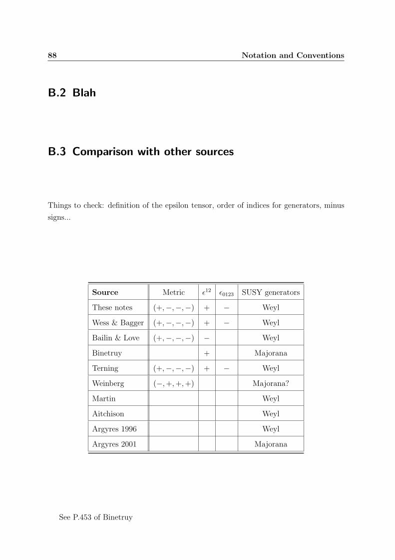
88 Notation and Conventions
B.2 Blah
B.3 Comparison with other sources
Things to check: definition of the epsilon tensor, order of indices for generators, minus
signs...
Source Metric ε12 ε0123 SUSY generators
These notes (+,−,−,−) + − Weyl
Wess & Bagger (+,−,−,−) + − Weyl
Bailin & Love (+,−,−,−) − Weyl
Binetruy + Majorana
Terning (+,−,−,−) + − Weyl
Weinberg (−,+,+,+) Majorana?
Martin Weyl
Aitchison Weyl
Argyres 1996 Weyl
Argyres 2001 Majorana
See P.453 of Binetruy
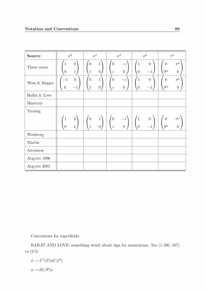
Notation and Conventions 89
Source σ0 σ1 σ2 σ3 γµ
These notes
1 0
0 1
0 1
1 0
0 −i
i 0
1 0
0 −1
0 σµ
σµ 0
Wess & Bagger
−1 0
0 −1
0 1
1 0
0 −i
i 0
1 0
0 −1
0 σµ
σµ 0
Bailin & Love
Binetruy
Terning 1 0
0 1
0 1
1 0
0 −i
i 0
1 0
0 −1
0 σµ
σµ 0
Weinberg
Martin
Aitchison
Argyres 1996
Argyres 2001
Conventions for superfields:
BAILIN AND LOVE: something weird about sign for momentum. See (1.166, 167)
vs (2.5)
φ→ U †(P )φU(P )
φ→ U(P)φ
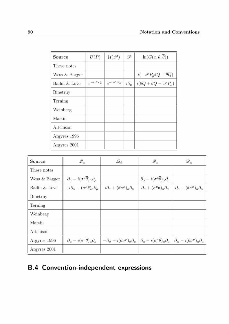
90 Notation and Conventions
Source U(P ) U(P) P ln(G(x, θ, θ))
These notes
Wess & Bagger i(−xµPµθQ+ θQ)
Bailin & Love e−ixµPµ e−ix
µPµ i∂µ i(θQ+ θQ− xµPµ)
Binetruy
Terning
Weinberg
Martin
Aitchison
Argyres 1996
Argyres 2001
Source Qα Qα Dα D α
These notes
Wess & Bagger ∂α − i(σµθ)α∂µ ∂α + i(σµθ)α∂µ
Bailin & Love −i∂α − (σµθ)α∂µ i∂α + (θσµ)α∂µ ∂α + (σµθ)α∂µ ∂α − (θσµ)α∂µ
Binetruy
Terning
Weinberg
Martin
Aitchison
Argyres 1996 ∂α − i(σµθ)α∂µ −∂α + i(θσµ)α∂µ ∂α + i(σµθ)α∂µ ∂α − i(θσµ)α∂µ
Argyres 2001
B.4 Convention-independent expressions
Appendix C
Useful Identities
“Insert quote.”
— Quote [2]
C.1 Pauli Matrices
...
C.2 Gamma Matrices
C.3 Fierz Identities
...
91
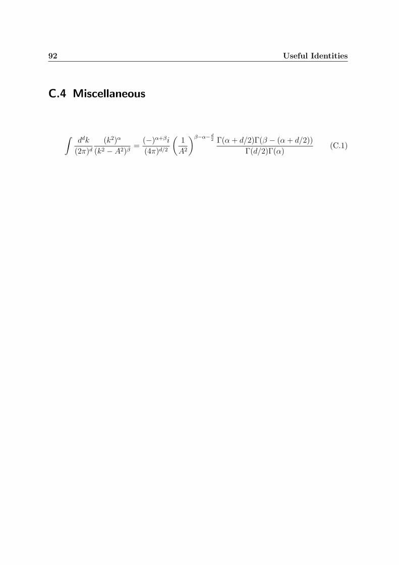
92 Useful Identities
C.4 Miscellaneous
∫ddk
(2π)d(k2)α
(k2 − A2)β=
(−)α+βi
(4π)d/2
(1
A2
)β−α− d2 Γ(α + d/2)Γ(β − (α + d/2))
Γ(d/2)Γ(α)(C.1)
Appendix D
Representations of the Poincare Group
“Insert quote.”
— Quote [2]
Here we present a more in-depth presentation of the representations of the Poincare
group, based on the lectures by Jan Gutowski (reference). For more information, the
reader is urged to see the relevant appendix of Wess and Bagger or Weinberg Volume I.
D.1 SL(2C)
2-1 relationship
D.2 Projective representations
Review Weinberg’s argument in detail here.
D.3 Further Reading
Choquet-Bruhat, Nakahara/Frankel, Moshe Carmeli, ...
93

94
Appendix E
Review of Gauge Theories
“Dimensions change as you change dimensions.”
— Hugh Osborn, Part III Advanced Quantum Field Theory 2007
This is a short review of relevant topics in gauge theory. This is neither meant to
be comprehensive nor succinct, it’s a subset of topics which the author felt was relevant
and/or interesting. Most of this treatment comes from [19] as well as the standard
Quantum Field Theory literature.
E.1 Lie Algebras
Caveat emptor. The following synopsis is meant to review the general idea of Lie
algebras and will not attempt to be mathematically rigorous. A more systematic and
mathematically honest treatment can be found in [10], from which this presentation
is condensed.
A Lie group, G, is a smooth, differentiable manifold which is also has a group structure.
In particular, the group multiplication of two elements of the manifold is a smooth map
and the inverse operator under this multiplication is also a smooth map. From differential
geometry we know that at each point, p, on the manifold we may define a set of tangent
vectors that span the n = dimG dimensional tangent space, Tp(G).
95
96 Review of Gauge Theories
These tangent vectors map real functions (f : U ∈ G → R) to R. Suppose γ(t) :
R → U ∈ G is a curve such that γ(0) = p. Then the tangent vector γp maps f →[ddt
(f γ(t))]t=0
.
The tangent space of a group is called its Lie algebra, which we shall denote L(G).
The Lie algebra of a group is equipped with a Lie bracket [ · , · ] : L(G)×L(G)→ L(G).
Lie algebra notation. When we discuss gauge groups, we really are interested in
Lie algebras.
For X, Y ∈ L(G)
E.2 Comparison with other sources
Appendix F
Review of Renormalization and
Effective Field Theory
“Q: What’s purple and changes with scale?
A: The renormalization grape.”
— Bastardization of a popular mathematics.
This is a summary of relevant ideas of the renormalization group and effective field
theory. Our prediction for new physics is based on the modern Wilsonian perspective of
renormalization.
There exist a few exceptionally intuitive expositions on the renormalization group.
These include the treatment based on dimensional analysis by Stevenson [20] and the
pedagogical approach to the Wilsonian paradigm by Hollwood [21]. In addition, many
modern quantum field theory texts (such as [9] and [22]) do a very good job explaining
renormalization.
F.1 Intuitive picture
F.2 Understanding UV divergences
Log log log.
97
98 Review of Renormalization and Effective Field Theory
F.3 Naturalness
Review of Renormalization and Effective Field Theory 99

100
Colophon
These notes were made in LATEX 2ε using KDE Integrated LATEX Environment [23] and
TextMate [24] the “hepthesis” class [25].
101

102
Bibliography
[1] F. Quevedo, Supersymmetry and extra dimensions, lecture notes taken by Philip
Tanedo, 2007, CASM ‘Part III’ course.
[2] G. Kane and M. Shifman, The Supersymmetric World: The Beginnings of the
Theory (World Scientific, 2000).
[3] I. L. Buchbinder and S. M. Kuzenko, Bristol, UK: IOP (1998) 656 p.
[4] E. D. Bolker, The American Mathematical Monthly 80, 977 (1973).
[5] H. K. Dreiner, H. E. Haber, and S. P. Martin, (2008), 0812.1594.
[6] H. J. W. Muller-Kirsten and A. Wiedemann, Print-86-0955 (KAISERSLAUTERN).
[7] J. Polchinski, Cambridge, UK: Univ. Pr. (1998) 531 p.
[8] S. Weinberg, Cambridge, UK: Univ. Pr. (2000) 419 p.
[9] S. Weinberg, The Quantum Theory of Fields, Vol I-III (Cambridge University
Press, 2005).
[10] J. Gutowski, Symmetries and particle physics, 2007, Michaelmas term Part III
course, Department of Applied Mathematics and Theoretical Physics, Cambridge
University.
[11] S. Weinberg, Cambridge, UK: Univ. Pr. (1995) 609 p.
[12] A. Salam and J. A. Strathdee, Phys. Rev. D11, 1521 (1975).
[13] A. Salam and J. A. Strathdee, Nucl. Phys. B76, 477 (1974).
[14] B. S. DeWitt, Supermanifolds , Cambridge, UK: Univ. Pr. (1992) 407 p. (Cambridge
monographs on mathematical physics). (2nd ed.),.
[15] F. Gieres, Lect. Notes Phys. 302, 1 (1988).
[16] M. Dine, Supersymmetry and string theory: Beyond the standard model , Cam-
bridge, UK: Cambridge Univ. Pr. (2007) 515 p.
[17] P. Binetruy, Supersymmetry: Theory, experiment and cosmology , Oxford, UK:
Oxford Univ. Pr. (2006) 520 p.
103
104 BIBLIOGRAPHY
[18] M. Puchwein and Z. Kunszt, Annals Phys. 311, 288 (2004), hep-th/0309069.
[19] H. Osborn and S. Gielen, Advanced quantum field theory, 2007, Lent term Part III
course, Department of Applied Mathematics and Theoretical Physics, Cambridge
University.
[20] P. M. Stevenson, Ann. Phys. 132, 383 (1981).
[21] T. Hollowood, Cut-offs and continuum limits: a wilsonian approach to field theory,
1998, Lecture Notes.
[22] M. Srednicki, Quantum Field Theory (Cambridge University Press, 2007).
[23] B. P. Jeroen Wijnhout, Holger Danielsson, Kde integrated LATEX environment,
2006.
[24] Micromates, Textmate: The missing editor, 2008.
[25] A. Buckley, The hepthesis LATEXbook class, 2007.
List of Figures
9.1 Examples of paths that are implicitly summed in equation (9.5). . . . . . 78
105

106
List of Tables
4.1 Representations of N > 1 SUSY. . . . . . . . . . . . . . . . . . . . . . . 52
107
Index
antisymmetric tensor, 13
Berezin integral, 57
BPS bound, 50
BPS state, 50
Casimir operator, 33
central charge, 31
chiral multiplet, 40
chirality, 21
coset, 54
coset space, 54
extended supersymmetry, 26
gauge multiplet, 40
gravity multiplet, 41
hypermultiplet
N = 2, 47
Lie algebra, 96
graded, 26
Lie bracket, 96
Lie group, 95
little group, 35
Lorentz group, 5
one-particle state, 35
Pauli matrix, 9
Pauli-Lubanski, 34
Poincare group, 5
R-symmetry, 30
SL(2,C), 8
conjugate representation, 12
contravariant representations, 15
fundamental representation, 12
spinor, 10
Dirac, 23
Majorana, 24
Weyl, 12
stability group, 35
supercharge, 26
superfield, 56, 61
superspace, 55
superspin, 41
vector multiplet
N = 2, 47
N = 4, 47
Witten index, 45
108