Supersymmetric Large

Extra Dimensions

Douglas Allan Hoover

Doctor of Philosophy

Physics Department

McGill University

Montreal, Quebec

2008-08-01

A thesis submitted to McGill University in partial fulfillment of the requirements ofthe degree of Doctor of Philosophy

Copyright c© Douglas Allan Hoover, 2008

DEDICATION

To Cole,

The world is a strange place; take pride in what you are able to understand,

but delight in the mystery that remains.

ii

ACKNOWLEDGEMENTS

There are a number of people to whom I am indebted, since without their

help this thesis would not have been completed. Foremost in this list is my thesis

supervisor, Cliff Burgess, who is one of the smartest people I have had the pleasure

of meeting. Ask him a question on any topic in physics, and besides giving you the

correct answer, you can expect at least one excellent physical reason why it has to be

so. I have also had the pleasure of working with some truly wonderful collaborators,

including Andrew Tolley, Claudia de Rham, and Gianmassimo Tasinato; I can only

hope that they gained as much from our collaborations as I did. I’d also like to thank

my fellow graduate student, Aristide Baratin, for his excellent translation of the thesis

abstract. I’d like to acknowledge Paula Domingues, the graduate secretary at McGill,

for her tremendous help in dealing with the administrative side of my degree. Of

course, this research was only possible because of generous financial support from

NSERC, McGill University, and Perimeter Institute. Much of the research for this

thesis was carried out at Perimeter Institute, and so I am grateful for their hospitality

during this time. On a more personal level, I would like to thank my parents for their

steadfast support and encouragement. They gave me the tools and the confidence

to succeed, and for that I am eternally grateful. Finally, I thank my wife Nicole, for

believing in me and for never once asking why in the world I work in six dimensions.

iii

CONTRIBUTION OF AUTHORS

This thesis contains portions of text from papers where the thesis author is a

co-author. Chapter 3 is an amalgamation of the papers [1] and [2]. Portions of

these papers to which the thesis author did not contribute have been removed, while

the remaining sections represent work to which the thesis author made significant

contributions. Chapter 4 contains work from [3], with contributions from the thesis

author in the majority of this work. Chapter 5 is taken virtually unaltered from

the paper [4], whose primary author is the thesis author. Chapter 6 is also an

amalgamation of results for two papers, [5] and [6]. Again, the thesis author is the

primary author of these papers.

iv

CONVENTIONS

Throughout this thesis, except where explicitly stated, we use the following con-

vention for the indices. Spacetime coordinates which run over the full dimensionality

of space are labeled generically by xM , with M = 0, 1, 2, 3, 5, 6, . . . (N.B. there is no

coordinate x4 in our convention), while coordinates referring to the four large dimen-

sions are labelled by greek indices, µ = 0, 1, 2, 3. As is customary, the coordinate x

with no index serves double-duty; at times, it refers to only the four large dimensions,

xµ, while at other times it refers to all spacetime coordinates, xM (if it is unclear

from the context, we write xµ or xM explicitly). To single out the coordinates of

the extra dimensions, we use ym with m = 5, 6, . . . . Tangent space indices will be

denoted by capital latin indices from the beginning of the alphabet, A, B, . . . .

Our metric and curvature conventions are the same as in Weinberg [7]. Specifi-

cally, our metric signature is mostly-plus, while the Riemann tensor is defined with

a relative minus sign compared with MTW [8], implying RMNPQ = −∂PΓM

NQ + . . . .

We work exclusively in units where ~ = c = 1, while at times we may also set either

κ2 = 8πGN or the Boltzmann constant k to unity. At various times, we’ll find it

convenient to write the metric as gMNdxMdxN = gµνdxµdxν + gmndymdyn. Thus,

when necessary to distinguish between quantities built out of gMN from those built

out of gµν , we use a caret. Similarly, tildes imply the object is built from the internal

metric, gmn. Finally, we reserve the coordinate r for Gaussian-Normal (GN) gauge,

defined such that the ‘internal’ metric is given by gmn = dr2 + habdzadzb.

v

ABSTRACT

In this thesis we examine the viability of a recent proposal, known as Supersym-

metric Large Extra Dimensions (SLED), for solving both the cosmological constant

and the hierarchy problems. Central to this proposal is the requirement of two

large extra dimensions of size rc ∼ 10 µm together with a low value for the higher-

dimensional scale of gravity, M∗ ∼ 10 TeV. In order not to run into immediate

conflict with experiment, it is presumed that all fields of the Standard Model are

confined to a four-dimensional domain wall (brane). A realization of the SLED idea

is achieved by relying on the 6D supergravity of Nishino and Sezgin (NS), which is

known to have 4D-flat compactifications.

When work on this thesis first began, there were many open questions which

are now answered either partially or completely. In particular, we expand on the

known solutions of NS supergravity, which now include: warped compactifications

having either 4D de Sitter or 4D anti-de Sitter symmetry, static solutions with bro-

ken 4D Lorentz invariance, and time-dependent “scaling” solutions. We elucidate

the connection between brane properties and the asymptotic form of bulk fields as

they approach the brane. Marginal stability of the 4D-flat solutions is demonstrated

for a broad range of boundary conditions. Given that the warped solutions of NS

supergravity which we consider are singular at the brane locations, we present an

explicit regularization procedure for dealing with these singularities. Finally, we de-

rive general formulae for the one-loop quantum corrections for both massless and

vi

massive field in arbitrary dimensions, with an eye towards applying these results to

NS supergravity.

vii

ABREGE

Cette these examine la viabilite d’une approche recente, dite des Dimensions

Supplementaires Larges Supersymetriques (Supersymmetric Large Extra Dimensions,

or SLED), qui propose une solution au probleme de la constante cosmologique et a

celui de la hierarchie. Un aspect central de cette approche est l’existence de deux di-

mensions supplementaires de grande taille rc ∼ 10 µm, et la faible valeur de l’echelle

de gravite, M∗ ∼ 10 TeV. Afin d’eviter un conflit immediat avec l’experience, tous

les champs du Modele Standard sont supposes etre confines dans les quatre dimen-

sions observees (i.e. sur une brane). Une implementation de cette idee de SLED est

realisee par le biais de la supergravite 6D de Nishino et Sezgin (NS), dont on sait

qu’elle a des compactifications 4D-plates.

Un certain nombre de questions, laissees ouvertes lorsque cette these a debutee,

sont a present partiellement ou completement resolues. En particulier, nous etendons

les solutions connues de la supergravite NS; elle incluent a present: compactifications

deformees ayant la symetrie de Sitter ou anti-de Sitter 4D, solutions statiques avec

invariance de Lorentz 4D brisee, et solutions d’echelle (“scaling”) dependentes du

temps. La relation entre les proprietes des branes et la forme asymptotique des

champs de bulk lorsqu’ils approchent la brane est mise en lumiere et expliquee. La

stabilite marginale des solutions 4D-plate est demontree pour une large classe de

conditions de bord. Etant donne que les solutions deformees de la supergravite NS

que l’on considere sont singulieres a l’emplacement de la brane, une procedure ex-

plicite de regularisation qui traite ces singularites est presentee. Enfin, des formules

viii

generales sont mises en place pour calculer les corrections quantiques a une boucle

pour des champs sans et avec masse en toute dimension, avec pour objectif a terme

d’appliquer ces resultats a la supergravite NS.

ix

TABLE OF CONTENTS

DEDICATION . . . . . . . . . . . . . . . . . . . . . . . . . . . . . . . . . . . ii

ACKNOWLEDGEMENTS . . . . . . . . . . . . . . . . . . . . . . . . . . . . iii

CONTRIBUTION OF AUTHORS . . . . . . . . . . . . . . . . . . . . . . . . iv

CONVENTIONS . . . . . . . . . . . . . . . . . . . . . . . . . . . . . . . . . . v

ABSTRACT . . . . . . . . . . . . . . . . . . . . . . . . . . . . . . . . . . . . vi

ABREGE . . . . . . . . . . . . . . . . . . . . . . . . . . . . . . . . . . . . . . viii

LIST OF TABLES . . . . . . . . . . . . . . . . . . . . . . . . . . . . . . . . . xiv

LIST OF FIGURES . . . . . . . . . . . . . . . . . . . . . . . . . . . . . . . . xv

1 Introduction . . . . . . . . . . . . . . . . . . . . . . . . . . . . . . . . . . 1

1.1 Effective Field Theory . . . . . . . . . . . . . . . . . . . . . . . . 31.1.1 EFT: An Overview . . . . . . . . . . . . . . . . . . . . . . 31.1.2 Technical Naturalness . . . . . . . . . . . . . . . . . . . . . 4

1.2 Two Troubling Naturalness Problems . . . . . . . . . . . . . . . . 71.2.1 The Hierarchy Problem . . . . . . . . . . . . . . . . . . . . 71.2.2 The Cosmological Constant Problem . . . . . . . . . . . . . 91.2.3 Naturalness: A Beacon in the Fog . . . . . . . . . . . . . . 12

1.3 Extra Dimensions . . . . . . . . . . . . . . . . . . . . . . . . . . . 131.3.1 Domain Walls & Branes . . . . . . . . . . . . . . . . . . . . 141.3.2 Kaluza-Klein Theory . . . . . . . . . . . . . . . . . . . . . 16

1.4 The SLED Proposal . . . . . . . . . . . . . . . . . . . . . . . . . . 201.4.1 Scale Invariance in SLED . . . . . . . . . . . . . . . . . . . 201.4.2 Why Large Extra Dimensions? . . . . . . . . . . . . . . . . 231.4.3 Why Supersymmetry? . . . . . . . . . . . . . . . . . . . . . 25

1.5 Thesis Summary . . . . . . . . . . . . . . . . . . . . . . . . . . . 28

x

2 6D Nishino-Sezgin Supergravity . . . . . . . . . . . . . . . . . . . . . . . 30

2.1 Nishino-Sezgin Supergravity . . . . . . . . . . . . . . . . . . . . . 312.2 Unwarped Solutions . . . . . . . . . . . . . . . . . . . . . . . . . . 34

2.2.1 Spherical Compactification . . . . . . . . . . . . . . . . . . 352.2.2 Rugby Ball . . . . . . . . . . . . . . . . . . . . . . . . . . . 40

2.3 Non-Supersymmetric Warped Solutions . . . . . . . . . . . . . . . 462.3.1 Uniqueness of Salam-Sezgin Vacuum . . . . . . . . . . . . . 492.3.2 General Axisymmetric Solutions . . . . . . . . . . . . . . . 512.3.3 Singularities of the GGP Solutions . . . . . . . . . . . . . . 55

3 New Solutions to 6D Supergravity . . . . . . . . . . . . . . . . . . . . . . 60

3.1 Asymptotic Near-Brane Geometries . . . . . . . . . . . . . . . . . 613.1.1 Asymptotics and Curvature . . . . . . . . . . . . . . . . . . 66

3.2 6D de Sitter Solutions . . . . . . . . . . . . . . . . . . . . . . . . 673.2.1 Equations of Motion . . . . . . . . . . . . . . . . . . . . . . 673.2.2 Solutions . . . . . . . . . . . . . . . . . . . . . . . . . . . . 68

3.3 Static Solutions with Broken 4D Lorentz Symmetry . . . . . . . . 733.3.1 Equations of Motion . . . . . . . . . . . . . . . . . . . . . . 733.3.2 Solutions . . . . . . . . . . . . . . . . . . . . . . . . . . . . 753.3.3 Asymptotic Forms . . . . . . . . . . . . . . . . . . . . . . . 77

3.4 Time-Dependent Scaling Solutions . . . . . . . . . . . . . . . . . . 783.4.1 Equations of Motion . . . . . . . . . . . . . . . . . . . . . . 803.4.2 Solutions . . . . . . . . . . . . . . . . . . . . . . . . . . . . 833.4.3 Useful Special Cases . . . . . . . . . . . . . . . . . . . . . . 853.4.4 Asymptotic Forms . . . . . . . . . . . . . . . . . . . . . . . 88

3.5 Discussion . . . . . . . . . . . . . . . . . . . . . . . . . . . . . . . 89

4 Perturbative Stability of the GGP Solutions . . . . . . . . . . . . . . . . 90

4.1 Equations of Motion . . . . . . . . . . . . . . . . . . . . . . . . . 914.1.1 Maximally Symmetric 4D Compactifications . . . . . . . . 93

4.2 Linearization . . . . . . . . . . . . . . . . . . . . . . . . . . . . . . 944.2.1 Symmetries and Gauge Choices . . . . . . . . . . . . . . . 944.2.2 Linearized Equations in Comoving Gauge . . . . . . . . . . 99

4.3 Properties of Solutions . . . . . . . . . . . . . . . . . . . . . . . . 1044.3.1 Analytic Solutions for General Conical Backgrounds . . . . 1044.3.2 Asymptotic Forms . . . . . . . . . . . . . . . . . . . . . . . 1064.3.3 Boundary Conditions and Brane Properties . . . . . . . . . 110

xi

4.4 General Stability Analysis . . . . . . . . . . . . . . . . . . . . . . 1134.4.1 Equations of Motion and Tachyons . . . . . . . . . . . . . . 1144.4.2 Action Analysis and Ghosts . . . . . . . . . . . . . . . . . 116

4.5 Discussion . . . . . . . . . . . . . . . . . . . . . . . . . . . . . . . 118

5 Regularization of Codimension-2 Brane Worlds . . . . . . . . . . . . . . 120

5.1 GGP Solutions Redux . . . . . . . . . . . . . . . . . . . . . . . . 1245.1.1 Capped Solutions . . . . . . . . . . . . . . . . . . . . . . . 127

5.2 Matching Conditions . . . . . . . . . . . . . . . . . . . . . . . . . 1305.2.1 Continuity Conditions . . . . . . . . . . . . . . . . . . . . . 1305.2.2 Jump Conditions . . . . . . . . . . . . . . . . . . . . . . . 133

5.3 Applications . . . . . . . . . . . . . . . . . . . . . . . . . . . . . . 1395.3.1 Capping a Given Bulk . . . . . . . . . . . . . . . . . . . . . 1395.3.2 Bulk Geometries Sourced by Given Branes . . . . . . . . . 1485.3.3 Volume Stabilization and Large Hierarchy . . . . . . . . . . 1555.3.4 Low-energy 4D Effective Potential . . . . . . . . . . . . . . 158

5.4 Discussion . . . . . . . . . . . . . . . . . . . . . . . . . . . . . . . 161

6 Ultraviolet Sensitivity in Higher Dimensions . . . . . . . . . . . . . . . . 163

6.1 General Results . . . . . . . . . . . . . . . . . . . . . . . . . . . . 1656.1.1 The Gilkey-DeWitt Coefficients . . . . . . . . . . . . . . . 1666.1.2 Dimensional Reduction from 6D to 4D . . . . . . . . . . . 1706.1.3 Brane-Localized Terms . . . . . . . . . . . . . . . . . . . . 175

6.2 Heat Kernel Coeffecients for Various Spin Fields . . . . . . . . . . 1796.2.1 Spin 0 . . . . . . . . . . . . . . . . . . . . . . . . . . . . . 1796.2.2 Spin 1/2 . . . . . . . . . . . . . . . . . . . . . . . . . . . . 1806.2.3 Spin 1 . . . . . . . . . . . . . . . . . . . . . . . . . . . . . 1826.2.4 Antisymmetric Tensors . . . . . . . . . . . . . . . . . . . . 1866.2.5 Spin 3/2 . . . . . . . . . . . . . . . . . . . . . . . . . . . . 1936.2.6 Spin 2 . . . . . . . . . . . . . . . . . . . . . . . . . . . . . 200

6.3 Supergravity Models . . . . . . . . . . . . . . . . . . . . . . . . . 2106.4 Application to Ricci Flat Backgrounds in 6D . . . . . . . . . . . . 214

6.4.1 Supersymmetric Multiplets . . . . . . . . . . . . . . . . . . 2166.4.2 Higher-Dimensional Field Content . . . . . . . . . . . . . . 221

6.5 Discussion . . . . . . . . . . . . . . . . . . . . . . . . . . . . . . . 224

7 Conclusions . . . . . . . . . . . . . . . . . . . . . . . . . . . . . . . . . . 226

xii

A Newton’s Law in Higher Dimensions . . . . . . . . . . . . . . . . . . . . 231

B Some Special Functions . . . . . . . . . . . . . . . . . . . . . . . . . . . 234

C Heat Kernel Calculations . . . . . . . . . . . . . . . . . . . . . . . . . . . 237

C.1 Antisymmetric Tensors . . . . . . . . . . . . . . . . . . . . . . . . 238C.2 Spin 3/2 . . . . . . . . . . . . . . . . . . . . . . . . . . . . . . . . 239C.3 Spin 2 . . . . . . . . . . . . . . . . . . . . . . . . . . . . . . . . . 241

D Gravitini with Λ 6= 0 . . . . . . . . . . . . . . . . . . . . . . . . . . . . . 243

REFERENCES . . . . . . . . . . . . . . . . . . . . . . . . . . . . . . . . . . . 250

xiii

LIST OF TABLESTable page

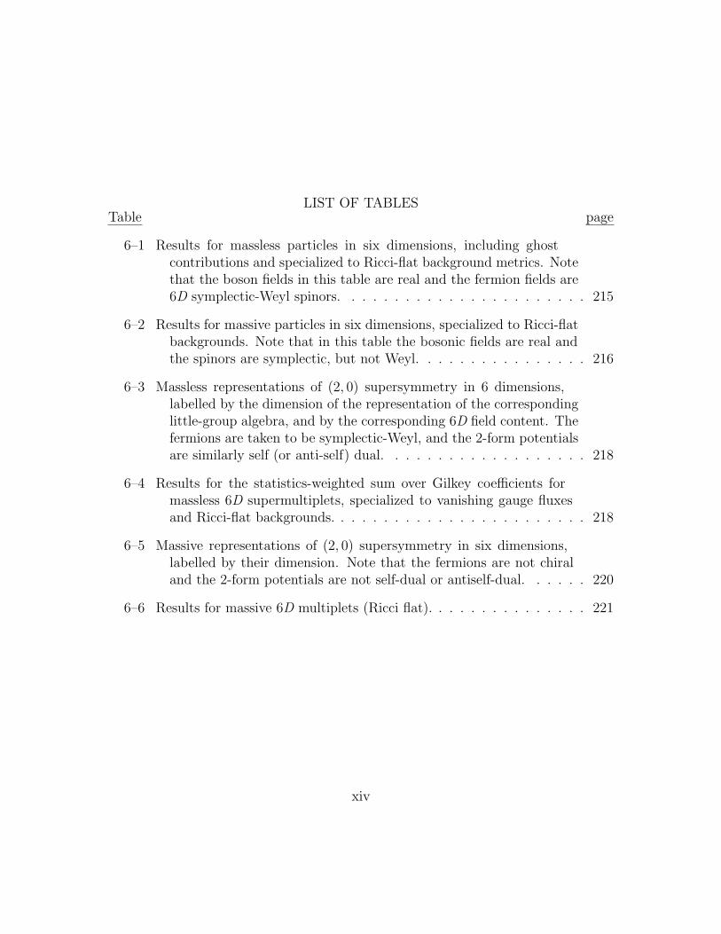
6–1 Results for massless particles in six dimensions, including ghostcontributions and specialized to Ricci-flat background metrics. Notethat the boson fields in this table are real and the fermion fields are6D symplectic-Weyl spinors. . . . . . . . . . . . . . . . . . . . . . . 215

6–2 Results for massive particles in six dimensions, specialized to Ricci-flatbackgrounds. Note that in this table the bosonic fields are real andthe spinors are symplectic, but not Weyl. . . . . . . . . . . . . . . . 216

6–3 Massless representations of (2, 0) supersymmetry in 6 dimensions,labelled by the dimension of the representation of the correspondinglittle-group algebra, and by the corresponding 6D field content. Thefermions are taken to be symplectic-Weyl, and the 2-form potentialsare similarly self (or anti-self) dual. . . . . . . . . . . . . . . . . . . 218

6–4 Results for the statistics-weighted sum over Gilkey coefficients formassless 6D supermultiplets, specialized to vanishing gauge fluxesand Ricci-flat backgrounds. . . . . . . . . . . . . . . . . . . . . . . . 218

6–5 Massive representations of (2, 0) supersymmetry in six dimensions,labelled by their dimension. Note that the fermions are not chiraland the 2-form potentials are not self-dual or antiself-dual. . . . . . 220

6–6 Results for massive 6D multiplets (Ricci flat). . . . . . . . . . . . . . . 221

xiv

LIST OF FIGURESFigure page

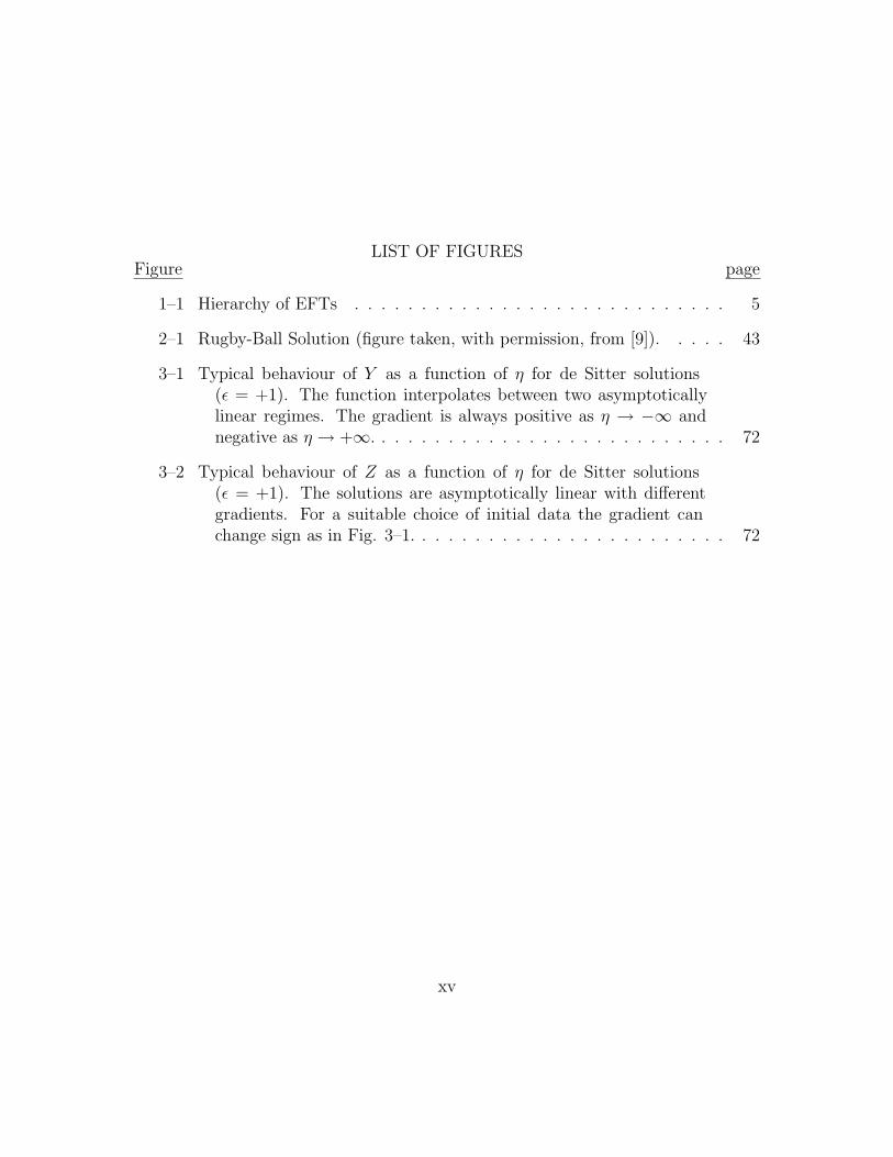
1–1 Hierarchy of EFTs . . . . . . . . . . . . . . . . . . . . . . . . . . . . 5

2–1 Rugby-Ball Solution (figure taken, with permission, from [9]). . . . . 43

3–1 Typical behaviour of Y as a function of η for de Sitter solutions(ε = +1). The function interpolates between two asymptoticallylinear regimes. The gradient is always positive as η → −∞ andnegative as η → +∞. . . . . . . . . . . . . . . . . . . . . . . . . . . 72

3–2 Typical behaviour of Z as a function of η for de Sitter solutions(ε = +1). The solutions are asymptotically linear with differentgradients. For a suitable choice of initial data the gradient canchange sign as in Fig. 3–1. . . . . . . . . . . . . . . . . . . . . . . . 72

xv

CHAPTER 1Introduction

The unprecedented success of both the particle physics Standard Model (SM)

and Einstein’s theory of General Relativity (GR) is both a blessing and a curse.

On the one hand, we have now confirmed aspects of the Standard Model to an

accuracy its inventors could scarcely have imagined forty years ago. One of its best

measured parameters, the fine structure constant α = 1/137.035 999 11(46) [10],

has been determined from a myriad of diverse experiments, including: precision

measurements of the anomalous magnetic moment of the electron, the quantum

hall effect, hyperfine splitting, low-energy atomic recoil measurements, high-energy

collider experiments, as well as many others [11]. Likewise, GR has withstood intense

experimental scrutiny, ranging from solar system tests, where it correctly predicts the

precession of Mercury’s orbit [12], to more exotic systems such as binary pulsars [13],

where the predicted rate of energy loss through gravitational waves is in excellent

agreement with observation [12].

On the other hand, there are compelling reasons to believe that the final theory

of everything is not so simple as SM + GR. Physicists thus find themselves in a

quandary, knowing current theories are inadequate yet without clear guidance from

experiment as to the nature of this final theory. There are hints, however, and these

come in the form of “naturalness” problems. As we describe in greater detail later,

one such naturalness problem suggests that General Relativity should be modified

1

at distances smaller than approximately 10 µm, while another advocates for a scale

of gravity much lower than the Planck mass. It is the position of this thesis that

both of these suggestions should be taken seriously. These ideas are embodied in the

Supersymmetric Large Extra Dimension (SLED) scenario, where it is assumed that

gravity is fundamentally six-dimensional with scale M∗ ∼ 10 TeV, only appearing

four-dimensional at distances much greater than 10 µm. Along with such a dramatic

modification comes a large number of experimental signatures, many of which will

be tested in upcoming experiments. In fact, it is a great virtue of this proposal that

it faces so many nontrivial tests in the near future. If it proves incorrect the damning

evidence will come swiftly and from many fronts, but should it succeed it will do so

spectacularly.

The remainder of this first chapter is organized as follows. In §1.1.1 we introduce

effective field theory and in §1.1.2 define what is meant by a naturalness problem. In

§1.2.1 and §1.2.2 we discuss two such naturalness problems: the hierarchy problem

and the cosmological constant problem. We then go on to argue in §1.3 that extra

spacetime dimensions can help with both of these problems. As in any theory with

extra dimensions, we must eventually be concerned with how the theory can appear

four-dimensional; this is the subject of domain walls, §1.3.1, and Kaluza-Klein reduc-

tion, §1.3.2. In §1.4 we introduce in earnest the SLED proposal, highlighting some

of its key features such as scale invariance, §1.4.1, large extra dimensions, §1.4.2,

and supersymmetry, §1.4.3. Finally, §1.5 provides a brief overview of the subsequent

chapters.

2

1.1 Effective Field Theory

Much of the work in this thesis relies, in some way or another, on concepts from

Effective Field Theory (EFT), and so in this section we provide a cursory overview

of the subject. For a more thorough treatment, the reader is instead referred to some

of the many excellent reviews, e.g. [14, 15].

1.1.1 EFT: An Overview

The credo of effective field theory is that to understand physics at one particular

scale, m, we’re not required to understand physics at the scales M m; indeed, if

this were not the case it’s hard to imagine how any progress in physics could be made

at all! Note that this does not imply that the high-energy physics is completely irrel-

evant, only that its effect on the low-energy theory is generically manifested through

a finite number of coupling constants. This phenomenon is known as decoupling.

The canonical example of an effective field theory is Fermi theory, which de-

scribes physics well below the mass the of the W boson, MW . Here, the effects

of W and Z bosons in fermion scattering ff → ff are accounted for by a four-

fermion interaction term in the Lagrangian, having coupling constant GF , and so

these bosons themselves no longer appear in the theory. We should expect that

this effective theory will be accurate up to corrections of order (Ecm/MW )n, where

Ecm is the centre-of-mass energy for the scattering process, and n is some integer.1

1 Should we desire a higher accuracy, corresponding to a larger n, we simply includehigher and higher dimension operators (e.g. a six-fermion interaction term) togetherwith their associated coupling constants.

3

If we happen to know the high-energy theory, we can calculate all the low-energy

coupling constants in terms of known parameters of the high-energy theory. On

the other hand, if we’re ignorant of the high-energy theory, then we must appeal to

experiment to determine these couplings.

Continuing in this manner, if we’re interested only in processes with an energy

much less than the muon mass, mµ, then there’s nothing to stop us from repeating

the above procedure. In this case, we remove from the Lagrangian all fields with mass

greater than or equal to mµ. As before, in order to account for the effects of the

fields we remove, we must add to our Lagrangian possible higher dimension operators

involving only low-energy fields.2 In this way, we arrive at the effective theory of

quantum electrodynamics (QED). Schematically, we have the following progression:

Standard Model→ Fermi Theory→ QED.

Of course, we could also go directly from the Standard Model to QED. This process

of successively removing heavy fields from our theory is referred to as integrating out

heavy degrees of freedom.

1.1.2 Technical Naturalness

We are now in a position to discuss the concept of technical naturalness [16].

Imagine for this purpose that we have a high-energy theory, valid at scale ΛHE, which

contains a light field ` having mass m ΛHE. Note that in this section, we are careful

2 As it turns out, QED is a renormalizable EFT, so there are no such higher-dimension operators in this case. This effective theory breaks down at energy 2mµ.

4

to distinguish between the bare mass, µ, which appears in the Lagrangian as µ2 `∗`,

and the physical mass, m, as measured by an experimentalist. At the classical level,

these two quantities are the same; however, taking into account radiative correction

from quantum mechanics, δµ2, we instead find m2 = µ2 + δµ2.

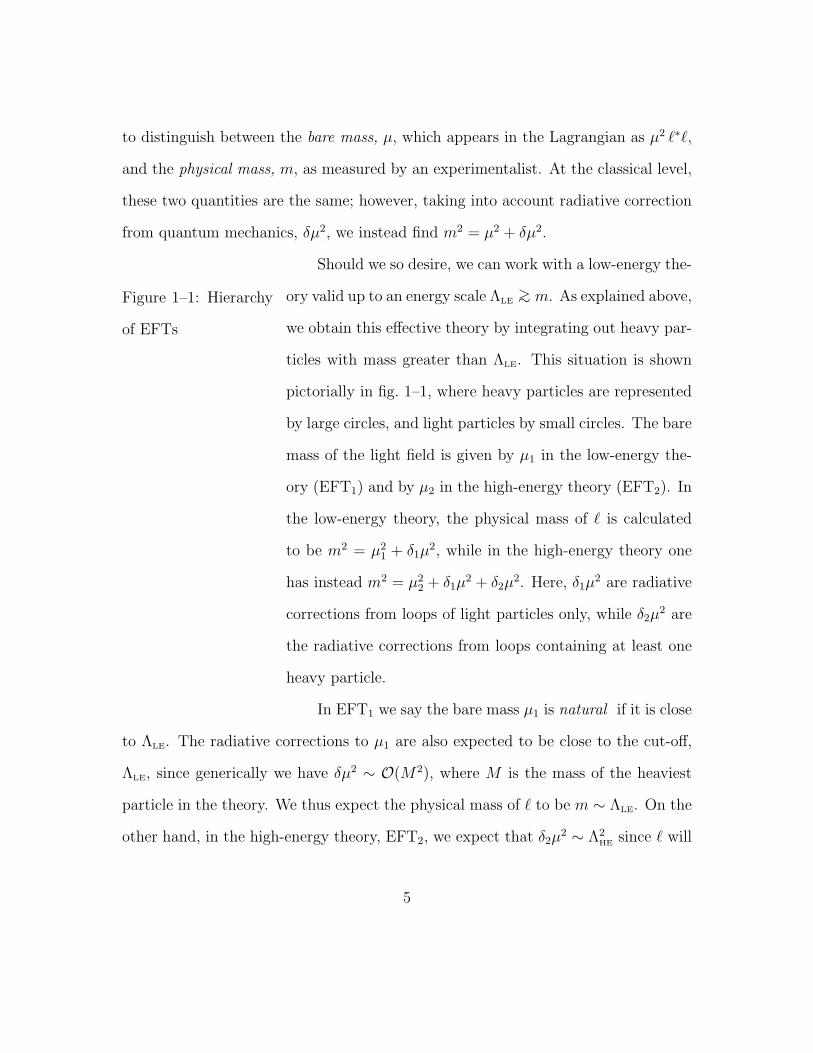
Figure 1–1: Hierarchy

of EFTs

Should we so desire, we can work with a low-energy the-

ory valid up to an energy scale ΛLE>∼ m. As explained above,

we obtain this effective theory by integrating out heavy par-

ticles with mass greater than ΛLE. This situation is shown

pictorially in fig. 1–1, where heavy particles are represented

by large circles, and light particles by small circles. The bare

mass of the light field is given by µ1 in the low-energy the-

ory (EFT1) and by µ2 in the high-energy theory (EFT2). In

the low-energy theory, the physical mass of ` is calculated

to be m2 = µ21 + δ1µ

2, while in the high-energy theory one

has instead m2 = µ22 + δ1µ

2 + δ2µ2. Here, δ1µ

2 are radiative

corrections from loops of light particles only, while δ2µ2 are

the radiative corrections from loops containing at least one

heavy particle.

In EFT1 we say the bare mass µ1 is natural if it is close

to ΛLE. The radiative corrections to µ1 are also expected to be close to the cut-off,

ΛLE, since generically we have δµ2 ∼ O(M2), where M is the mass of the heaviest

particle in the theory. We thus expect the physical mass of ` to be m ∼ ΛLE. On the

other hand, in the high-energy theory, EFT2, we expect that δ2µ2 ∼ Λ2

HE since ` will

5

generically couple to particles with mass of order ΛHE. Thus, in order to maintain

a small physical mass, we must choose µ22 to be very nearly equal to −δ2µ

2 in order

that their sum be O(m2) Λ2HE. This is an example of fine-tuning. Alternatively,

it could be that there is a symmetry which prevents radiative corrections from being

as large as O(M2) in which case no fine-tuning is required to maintain the hierarchy

mM : we say that the hierarchy is technically natural. What’s more, we demand

a technically natural understanding of the given hierarchy at any energy scale (e.g.

EFT1 or EFT2).

As an example of a technically natural hierarchy, consider the electron in the

Standard Model, with mass me MW . This hierarchy is technically natural because

radiative corrections to the electron’s mass are suppressed by an approximate chiral

symmetry,

ψe → eiαγ5ψe, (1.1)

which is broken by the term µ ψeψe, where for our purposes here µ is just a constant

(analogous to bare mass discussed earlier). Here, α = α(x) is an arbitrary function

and γ5 is the usual chirality matrix. Chiral symmetry implies that corrections to the

electron mass must vanish as µ→ 0, from which we conclude that these corrections

are proportional to µ. In fact, detailed calculation shows that at one-loop δµ ∝

µ ln(M/µ), where M is the mass of some heavy particle. Given that µM , we see

that the radiative corrections also satisfy δµM and so this hierarchy is technically

natural, as claimed.

While the preceding discussion focused on naturalness as it pertains to mass,

this can be easily generalized to other couplings. Given an EFT with a cut-off ΛUV,

6

any bare coupling can be written as g0 · ΛnUV, where g0 is dimensionless and n is an

integer chosen to ensure correct dimensions. If the corresponding physical coupling

g is measured and found to satisfy g 1, then naturalness requires two conditions:

(i) that the smallness of g0 be understood within the microscopic theory, and (ii)

that radiative corrections to g0 also be small.

1.2 Two Troubling Naturalness Problems

In this section, we introduce both the hierarchy problem and the cosmological

constant problem. Roughly speaking, the hierarchy problem is the question of how

the hierarchy MEW MPl can be technically natural given that the scale of elec-

troweak symmetry breaking, MEW, is assumed to be set by the mass of a scalar field,

the Higgs, whose radiative corrections should demand that MEW ∼ MPl. The cos-

mological constant problem is the disparity between vacuum energy we expect from

calculating loops of heavy particles, and the vacuum energy we actually observe.

Both are examples of fine-tuning problems, as we now discuss.

1.2.1 The Hierarchy Problem

The Higgs field is an as-yet-unobserved scalar doublet φ which is the postulated

source of mass within the Standard Model. Its potential is given by

V (φ) = λ(φ†φ− µ2/2λ)2, (1.2)

implying that it has a bare mass m20H = 2µ2. In the case of the Higgs field, we note

that there is no approximate symmetry (analogous to chiral symmetry for fermions)

which can protect its mass from receiving large corrections.

7

The hierarchy problem now stems from two basic facts. First, there is a general

consensus among theorists that the Standard Model must be treated as an effec-

tive field theory. That the Standard Model is not a complete theory is itself not

a surprise, as it already contains a glaring omission — gravity! However, we might

assume that it is at least valid up to some intermediate ‘Grand Unified’ (GUT) scale,

MGUT ∼ 1016 GeV. Second, in the Standard Model, electroweak symmetry breaking

is assumed to occur through a process whereby a scalar field — the Higgs — obtains

a vacuum expectation value. As it stands, there is now overwhelming evidence that

the electroweak symmetry breaking should occur at the scale MEW ∼ 1 TeV, and

thus the Higgs mass also needs to be mH<∼ 1 TeV [10]. To see how this leads to a

naturalness problem, we imagine calculating the Higgs mass within the high-energy

GUT theory. This is the same situation described in the previous section, and so we

expect

m2H = m2

0H + δm2H (1.3)

where the radiative corrections δm2H are expected to be of order M2

GUT. Given that

mH is order TeV, we see that the bare mass m20H must be fine-tuned to order 1 part

in 1026.

Notice that the existence of this fine-tuning presupposes that the Higgs descrip-

tion of electroweak symmetry breaking is correct. Since the Higgs field has not yet

been observed, it is reasonable to question whether this simple description is re-

ally correct. For example, it could be that the Higgs is not a fundamental scalar,

as postulated by Technicolor theories [17, 18]. Alternatively, even if the Standard

Model Higgs is the correct low-energy description, it could happen that new particles

8

emerge at the TeV scale which work to suppress the radiative corrections to m2H , as

happens in the Minimal Supersymmetric Standard Model [19].

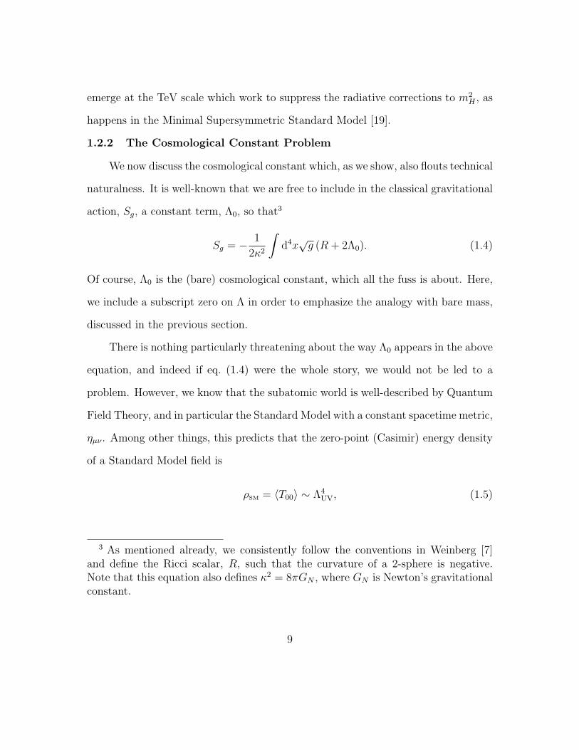
1.2.2 The Cosmological Constant Problem

We now discuss the cosmological constant which, as we show, also flouts technical

naturalness. It is well-known that we are free to include in the classical gravitational

action, Sg, a constant term, Λ0, so that3

Sg = − 1

2κ2

∫d4x√g (R + 2Λ0). (1.4)

Of course, Λ0 is the (bare) cosmological constant, which all the fuss is about. Here,

we include a subscript zero on Λ in order to emphasize the analogy with bare mass,

discussed in the previous section.

There is nothing particularly threatening about the way Λ0 appears in the above

equation, and indeed if eq. (1.4) were the whole story, we would not be led to a

problem. However, we know that the subatomic world is well-described by Quantum

Field Theory, and in particular the Standard Model with a constant spacetime metric,

ηµν . Among other things, this predicts that the zero-point (Casimir) energy density

of a Standard Model field is

ρSM = 〈T00〉 ∼ Λ4UV, (1.5)

3 As mentioned already, we consistently follow the conventions in Weinberg [7]and define the Ricci scalar, R, such that the curvature of a 2-sphere is negative.Note that this equation also defines κ2 = 8πGN , where GN is Newton’s gravitationalconstant.

9

where ΛUV is the ultraviolet (UV) cut-off where the theory is expected to break

down, and Tµν is the Energy-Momentum tensor for the field in question. Unbroken

Lorentz invariance necessarily implies that 〈Tµν〉 is proportional to ηµν , and so we

have 〈Tµν〉 = −ρSMηµν . Coupling this theory to gravity in the usual way, one obtains

that the vacuum field equations obey: Gµν − Λ0gµν = −κ2〈Tµν〉 = κ2ρSM gµν . Notice

that we can define the physical cosmological constant,

Λ = Λ0 + κ2ρSM (1.6)

in which case the Einstein equation becomes

Gµν − Λ gµν = 0. (1.7)

Just as it is physical mass and not the bare mass which is measured in particle

physics experiments, it is this physical cosmological constant which is directly mea-

surably from cosmological observations. Evidence from such observations, including

the cosmic microwave background (CMB) [20, 21] and Type 1a supernovae [22, 23,

24], implies that Λ is given by

κ−2Λ ≈ (10−12 GeV)4. (1.8)

For later discussions, it is useful to define what we call the vacuum energy density —

also known as dark energy — which is simply ρvac = κ−2Λ. Notice that the vacuum

energy, ρvac, includes contributions from the bare cosmological constant, Λ0 as well

as radiative corrections from all matter fields, ρSM.

10

To understand why this leads to a problem, we note that any reasonable estimate

for ρSM gives an answer many orders of magnitude larger than this observed value for

Λ. For example, an upper bound on this quantity is obtained by taking the cut-off

to be the Planck scale, MPl, giving ρSM ∼ M4Pl = (1018 GeV)4. A more conservative

estimate takes the cut-off to be the scale of electroweak symmetry breaking, MEW, in

which case we find ρSM ∼M4EW = (103 GeV)4 — still many orders of magnitude larger

than the observational bound. In fact, any particle physics scale (except perhaps

neutrino masses) inserted into eq. (1.5) gives a contribution which is much larger

than the observed vacuum energy, ρvac. Similarly to the hierarchy problem, we must

fine-tune parameters in order to enforce a small physical cosmological constant. For

example, taking the cut-off as MEW, we see that the cancellation between Λ0 and ρSM

in eq. (1.6) must be exact to 1 part in 1060! Certainly, it is very unnatural to expect

that these two quantities, which have nothing apparently to do with one another,

should be so very nearly equal.

Despite the similarities with the hierarchy problem, the cosmological constant

problem is worse by far. While the existence of the hierarchy problem relies on what

we expect physics to be above the TeV scale, the cosmological constant problem

can be phrased in terms of physics we think we understand. For example, we can

choose to calculate the cosmological constant within the effective theory of QED.

There, we find that electron loops contribute to the vacuum energy an amount of

order m4e Λ. Thus, even in a theory such as QED which we understand well, it is

necessary to fine-tune parameters.

11

1.2.3 Naturalness: A Beacon in the Fog

Our discussion thus far belies the fact that technical naturalness is ubiquitous

in nature. In all but a handful of cases, e.g. the hierarchy and cosmological con-

stant problem, a large hierarchy of scales can be understood in a technically nat-

ural way [25]. (Indeed, if that were not the case, few physicists would lose sleep

over fine-tuning.) Even so, the egregiousness of the cosmological constant problem

has led some to abandon technical naturalness as a useful principle [26, 27]. This

attitude, which also goes under the name of the Anthropic Principle, was first le-

gitimized through Weinberg’s famous prediction for the value of the cosmological

constant [28]. The anthropic principle has also undergone a recent revival thanks to

ideas from string theory [27].

In this thesis we do not take such an attitude; in stark contrast, we hold technical

naturalness as our guiding light. The benefit of this approach is immediate, since it

allows us to infer that something peculiar must happen at around the dark energy

scale, ρvac ∼ (10−3 eV)4. Treating this scale as a physical cut-off, we see that below

ρvac the cosmological constant in the corresponding low-energy EFT is naturally the

correct order of magnitude. However, if the theory above this scale is the Standard

Model together with General Relativity, then we have already seen that fine-tuning

problems arise. Given that the Standard Model is tightly constraint below 1 TeV, we

conclude that it is General Relativity that must be modified within this range. As

we discuss shortly, SLED is perhaps the simplest scenario for how gravity is modified

at the dark energy scale. There are other proposals which take a similar tack, for

example postulating that gravity is a composite particle [29]. However, we argue that

12

SLED is the most promising such proposal as it can be realized within a fully-fledged

microscopic model which is valid all the way up to the weak scale.

1.3 Extra Dimensions

As mentioned at the start of this chapter, the modification to gravity which

SLED proposes is the addition of two large extra dimensions, with Standard Model

fields trapped on a four-dimensional surface. Before getting into the details, however,

we first pause to motivate why extra dimensions might be useful for solving the two

aforementioned problems. Because in SLED gravity is not fundamentally 4D, this in

turn implies that neither is the 4D Planck mass, MPl, fundamental. If, as proposed

by SLED, the fundamental scale of gravity is instead M∗ ∼ 10 TeV, then new physics

could begin to appear at around the TeV scale. Accordingly, the physical cut-off for

the Standard Model would also be around 1 TeV and so the Higgs mass would be

technically natural.

With regard to the cosmological constant problem, recall we showed that 4D

Lorentz invariance implies that gravity responds to the zero point energy of a quan-

tum field as if it were a cosmological constant, cf. eq. (1.6). Extra dimensions change

this story in two fundamental ways: first, there is obviously no requirement for 6D

Lorentz invariance; and second, because Standard Model fields are assumed to be

trapped on a lower-dimensional surface, their Casimir energy acts not as a 6D cos-

mological constant but rather as an energy density which is localized in the extra

dimensions. In chapter 2 we show explicitly how these two loopholes are exploited.

Having established the case for extra dimensions, we now discuss some of the

more technical details. In §1.3.1 we argue that mechanisms exist to trap the Standard

13

Model fields on a sub-surface (brane) within a higher-dimensional spacetime, which

is an essential component of the SLED proposal. Given that gravity cannot similarly

be trapped, we discuss in §1.3.2 how gravity appears to a low-energy observer on a

brane and how it can be that this situation is not already ruled out experimentally.

1.3.1 Domain Walls & Branes

The idea that the universe may have more than four dimensions is an old one,

attributed to Kaluza [30] and Klein [31]. While this may seem contradictory to

our everyday experience, there are in fact two basic mechanisms one can employ in

order not to run into conflict with experiment (in general, a given model will employ

some combination of these two mechanisms). The simplest is to assume that the

extra dimensions are very small, having “compactification radius” rc, in which case

the effect of the extra dimensions is negligible at energies much less than r−1c (this

statement is made more precise in §1.3.2). Here, we are assuming that the extra

dimensions are universal, meaning fields propagate freely in all dimensions. Within

this picture, we must have r−1c

>∼ TeV which is above the energy scale currently

probed by colliders.

Alternatively, one can assume that fields are trapped on a lower-dimensional

surface (domain wall) while only gravity is free to propagate within the full dimen-

sionality of spacetime. This is the picture suggested by string theory, where these

lower-dimensional surfaces are generically referred to a p-branes, with p being the

spatial dimension of the brane. Notice that because fields can be localized to 3 spa-

tial dimensions, the extra dimensions can be taken to be large (or infinite). We point

out that it’s really only necessary to trap the Standard Model fields onto a 3-brane;

14

“bulk” fields can freely propagate in the large extra dimensions without immediate

problems.

String Theory Branes

In string theory, Dirichlet p-branes are extended objects onto which open strings

can end (see [32] for a pedagogical introduction). Thus, string theory provides a

natural mechanism with which to localize objects onto a lower-dimensional manifold.

It is also true that gravitons in string theory are described by closed strings, and as

such they cannot be localized in the same way that open strings can. This should be

expected since gravity can be interpreted as the curvature of space, and so intuitively

gravitons must be free to propagate in all dimensions.

For the most part, however, we are not concerned with the string theory origin

of branes. The main reason for this is that it much more convenient to be able to

choose for ourselves brane properties, such as their couplings to the dilaton, gauge

fields, etc., as opposed to using those dictated by string theory. Of course, it would

be desirable to eventually have a string theory derivation, but for now we content

ourselves with this more pragmatic approach.4

Field Theory Domain Walls

Even within humble field theory it is possible to trap fields on domain walls,

which we also refer to as branes although they need not have any assumed connection

to string theory (thus, unless otherwise indicated, “domain wall” and “brane” should

4 A string theory derivation of the 6D supergravity which we focus on in this thesisis given in [33].

15

be taken as synonymous). For example, we can consider the action

S =

∫dp+1x ddyLbulk(Φ(x, y)) +

∫dp+1xLbrane(Φ(x, 0), φ(x)), (1.9)

where Φ(x, y) and φ(x) symbolize any number of bulk fields and brane fields, re-

spectively, and we have used our coordinate freedom to place the p-brane at the

bulk location y = 0. The simplest action for the brane is one due to pure tension,

corresponding to a Lagrangian Lbrane = −√hT with hab the induced metric on the

brane and T its tension.

Starting from this action, one can derive equations of motion from the usual vari-

ational principle, although slightly more care must be taken because of the explicit

boundary term. For the codimension-1 case (d = 1 in the above action), this proce-

dure leads to solutions which are generically well-defined at y = 0. However, as we

discuss in greater detail in subsequent chapters, the case d ≥ 2 can be problematic.

1.3.2 Kaluza-Klein Theory

Since gravity must propagate in all dimensions, one might wonder how it can be

that extra dimensions (of any size and number) are not already ruled out by gravita-

tional experiments. To be more precise, we should ask why low-energy experiments

have not ruled out this situation. To answer this question we construct the effective

4D theory relevant to the low-energy observer, which we do in two steps. First, we

show that the 6D theory is exactly equivalent to a 4D theory, albeit with an infinite

number of particles in the 4D version. Second, we integrate out all but the massless

modes of the exact 4D theory to obtain the effective 4D theory. We go through this

16

calculation in some detail, as the lessons learned will be important for SLED (and,

indeed, any other theory with extra dimensions).

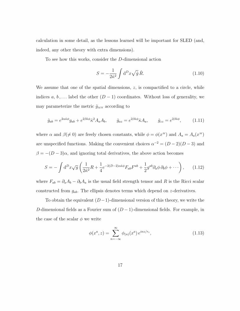
To see how this works, consider the D-dimensional action

S = − 1

2κ2

∫dDx

√g R. (1.10)

We assume that one of the spatial dimensions, z, is compactified to a circle, while

indices a, b , . . . label the other (D − 1) coordinates. Without loss of generality, we

may parameterize the metric gMN according to

gab = e2ακφgab + e2βκφκ2AaAb, gaz = e2βκφκAa, gzz = e2βκφ, (1.11)

where α and β( 6= 0) are freely chosen constants, while φ = φ(xM) and Aa = Aa(xM)

are unspecified functions. Making the convenient choices α−2 = (D− 2)(D− 3) and

β = −(D − 3)α, and ignoring total derivatives, the above action becomes

S = −∫

dDx√g

(1

2κ2R +

1

4e−2(D−2)ακφFabF

ab +1

2gab∂aφ ∂bφ+ · · ·

), (1.12)

where Fab = ∂aAb − ∂bAa is the usual field strength tensor and R is the Ricci scalar

constructed from gab. The ellipsis denotes terms which depend on z-derivatives.

To obtain the equivalent (D−1)-dimensional version of this theory, we write the

D-dimensional fields as a Fourier sum of (D− 1)-dimensional fields. For example, in

the case of the scalar φ we write

φ(xa, z) =∞∑

n=−∞

φ(n)(xa) einz/rc , (1.13)

17

where rc is the radius of the circle, so that 0 ≤ z < 2πrc. Our assertion is that

fields with n 6= 0 represent massive fields in the lower-dimensional theory, and so

can be integrated out from the low-energy theory. To justify this claim, consider the

simpler toy model of a single massless scalar field which we Fourier decompose as

above. When we integrate over the extra dimension, we obtain the result

S = −∫

dDx ∂Mφ ∂Mφ = −(2πrc)

∑n

∫dD−1x

[∂aφ(n)∂

aφ(n) +

(n

rc

)2

φ2(n)

]. (1.14)

Indeed, we see that the fields φ(n) have mass m(n)= (n/rc) in the lower-dimensional

theory.

Performing the analogous Fourier decomposition and integration in the action

(1.12), we obtain a (D− 1)-dimensional theory involving both massive and massless

fields, with complicated interactions. Integrating out these massive fields at the

classical level amounts to using the equations of motion to eliminate these fields

from the action. In the limit where the Kaluza-Klein mass goes to infinity, this

amounts to a truncation to the massless sector, in which case we may substitute in

the solutions φ(n6=0) = 0, gab(n6=0) = 0, and Aa(n6=0) = 0. The result of this procedure is

the (D − 1)-dimensional action

S = −∫

dD−1x√g

(1

2κ2R(0) +

1

4e−4ακφ(0)F(0) abF

ab(0) +

1

2∂aφ(0) ∂

aφ(0)

), (1.15)

where the length, L = 2πrc, of the extra dimension has been absorbed by a constant

field redefinition of φ(0) and Aa(0), and we include the zero subscript to emphasize

that these are massless modes. Notice that we have made the definition κ2 = κ2/L,

and that the fields depend only on xa.

18

Take-home Messages

There are several noteworthy features of the above Kaluza-Klein reduction.

First, we see that eq. (1.15) must be viewed as an effective action whose physical

cut-off is given by the lowest non-zero Kaluza-Klein (KK) mass, m(1) = 1/rc. Above

this scale, no effective field theory description exists for the simple reason that there

is no large hierarchy of scales (the ratio between two successive KK levels is always

O(1), except between n = 0 and n = 1). Of course, in more complicated situations

the KK spectrum will not be so simple, although the moral will almost always be

the same: above the KK scale we forced to work with the higher dimensional theory.

We also note here that it is a typical feature of dimensional reduction that massless

fields (besides the graviton) appear in the lower-dimensional theory. Since massless

fields can have potentially interesting cosmological implications, a careful treatment

of their effects is usually warranted.

We also learn how the fundamental scale of gravity is related to the lower-

dimensional scale measured in the effective field theory. For example, specializing

to the case D = 5, the above analysis shows that the 5D Planck mass, M3∗ = 1/κ2,

is related to the usual 4D Planck mass by M3∗L = M2

Pl. It is straightforward to

generalize this result to the case where there are d extra dimensions. To do so, we

use the metric ansatz

gMNdxMdxN = gµν(x)dxµdxν + gmn(y)dymdyn. (1.16)

19

From this, it follows that the gravitational action reduces to

Sg = −1

2M2+d∗

∫ddy√g

∫d4x√gR(x) + · · · = −1

2(M2+d∗ Vd)

∫d4x√gR(x) + · · ·

where the ellipses denote y-dependent quantities. To obtain the second equality we

have integrated over the extra dimensions, yielding the d-dimensional volume factor,

Vd. We thus find that the 4D Planck mass is related to M∗ via

M2+d∗ Vd = M2

Pl. (1.17)

In §1.4, we show how this result can be exploited in order to solve — or, at least,

rephrase — the hierarchy problem.

1.4 The SLED Proposal

Having covered the necessary background, we are now in a position to introduce

the SLED proposal. To start, we discuss scale invariance and the role it plays in

ensuring that the 4D effective vacuum energy vanishes classically. We next introduce

the Large Extra Dimension (LED) scenario of Arkani-Hamed, et al. [34, 35] which

addresses the hierarchy problem. Next, we introduce supersymmetry, motivated by

the fact that this symmetry promotes the LED scenario to a possible solution to both

the cosmological constant problem and the hierarchy problem.

1.4.1 Scale Invariance in SLED

In this section, we define scale invariance and show why it is important for

SLED. A scale transformation is nothing but a rescaling of the metric, so its action

on the metric can be represented as

gMN → eσgMN (1.18)

20

where σ is a constant. In general, other fields may also transform; for example,

there is often a scalar field — the dilaton — which shifts by a constant which is

proportional to σ, e.g.

ϕ→ ϕ− σ. (1.19)

Given an action, S =∫

dDxL(gMN , φ, . . .), where the ellipsis denotes the other

fields in the theory (which may or may not transform under the above scale trans-

formation), we say that the theory is scale invariant if the action transforms as

S → const.×S. Since equations of motion are unchanged by a constant rescaling of

the action, we see that given any solution to the equations of motion a one-parameter

family of new solutions can be generated by application of a scale transformation.

In the context of SLED, we now ask what scale invariance implies for the vacuum

energy in the 4D effective theory, whose calculation was considered in §1.3.2. To

proceed, we need to evaluate the on-shell action, Scl, obtained by evaluating the

action assuming all fields obey their classical equations of motion. Scale invariance

allows Scl to be written in the following equivalent ways:

Scl =

∫dDxL(gcl

MN , φcl, . . .) = e−ωBσ

∫dDxL(eσ gcl

MN , φcl − σ, . . .), (1.20)

where the last equality assumes S transforms to eωB σS under a scale transformation.

Here, ωB is a constant which is easily determined once the functional form of the

action is given (the actions we encounter in later chapters have ωB = 2). Notice

that we consider here the case where spacetime has no boundaries; the general result

including boundaries is a straightforward generalization [36]. Noting that the middle

equality in eq. (1.20) is independent of σ, we differentiate this equation with respect

21

to σ and then set σ = 0 to obtain the result

0 = −ωBScl +

∫dDx

[δScl

δgclMN

gclMN −

δScl

δφcl+ · · ·

]. (1.21)

Notice that each term in the above integral individually vanishes as the fields are

assumed to satisfy the classical equations of motion. Thus, we obtain the important

result ωBScl = 0, which for ωB 6= 0 implies that the on-shell action, Scl, vanishes. In

the case where there are boundary branes bi — whose actions transform under a scale

transformation as Sbi → eωbiσSbi — we again find Scl = 0 provided ωB = ωbi 6= 0.

To see what this result implies for the vacuum energy in the 4D effective theory,

we consider integrating out all massive modes. As described earlier, at the classical

level this is accomplished by using the classical equations of motion to eliminate

these modes from the action. For the purpose of calculating the 4D vacuum energy,

it suffices to consider the case where all fields are independent of xµ, in which case

we find

ρeff =

∫ddyLcl ∝ Scl = 0. (1.22)

Thus, we see that unbroken scale invariance ensures that the 4D vacuum energy

vanishes. One might nonetheless worry that since scale invariance is a symmetry of

the equations of motion and not of the action, we should expect this “symmetry”

to be broken by quantization. Indeed, it is the task of supersymmetry (discussed

shortly) to ensure that the scale of breaking is given by the supersymmetry breaking

scale, which is typically small in the cases of interest.

22

1.4.2 Why Large Extra Dimensions?

We have already seen that a natural solution to the cosmological constant prob-

lem suggests that gravity is fundamentally modified at the scale ρvac — a fact that

can be easily accommodated by having extra dimensions with size ρ−1vac. We now show

that the hierarchy problem can also be solved using large extra dimensions. Remark-

ably, for the case of two extra dimensions, the size of the dimensions required to solve

the hierarchy problem is also ρ−1vac.

The LED scenario relies on the observation made in §1.3.2 that the higher-

dimensional scale of gravity is related to the 4D Planck mass by the equation5

M2+d∗ Vd = M2

Pl. (1.23)

This equation suggests a novel solution to the hierarchy problem: assume M∗ ∼

TeV! Given that the MPl ∼ 1018 GeV, eq. (1.17) implies that the size of the extra

dimensions is very large relative to M−1∗ . We see that the LED scenario solves the

hierarchy problem in a trivial way, since it assume that there is only one fundamental

scale, MEW. To be fair, the hierarchy problem has not really disappeared, but rather it

has been transmuted to the question of whether large extra dimensions, viz. Md∗ Vd

1, can be technically natural.

Substituting in numbers, one finds that for one extra dimension its size must

be rc ∼ 1013 cm ∼ 1 AU in order to have TeV-scale gravity. Not surprisingly, this

5 Among other things, this result assumes that our four large dimensions are notstrongly “warped”, a concept introduced in §2.3.

23

situation is empirically ruled out by solar system tests. On the other hand, for d = 2

one finds that the choice M∗ ∼ 10 TeV leads to extra dimensions of size rc ∼ 10µm ∼

(10−2 eV)−1. Again, one can ask whether this situation is observationally excluded,

although here the answer is less obvious.

We know that Standard Model processes are sensitive to the dimensionality of

space, and since the (4D) Standard Model has been confirmed down to a distance

of roughly TeV−1 its fields must be confined to a 4D brane. Even though Standard

Model fields are confined to a brane, there can still be observable signatures in col-

lider experiments since these fields must interact with gravity, which is not similarly

confined. Thus, there will be “missing energy” signatures coming from decays of

Standard Model particles into unobserved Kaluza-Klein modes of the graviton, for

example

e+ + e− → γ +GKK .

The low scale of quantum gravity, M∗, also implies that virtual graviton exchange

could lead to dangerous corrections to well-measured Standard Model processes.

Considerations such as these lead to a collider physics bound M∗ >∼ 1 TeV [37, 38, 39].

Because gravity is not trapped on a brane, we must ask whether precision tests

of gravity have already ruled out large extra dimensions. As shown in appendix A,

for d extra dimensions of size rc the gravitational force between objects separated

by a distance r rc obeys the usual inverse square law (ISL), varying as 1/r2; at

distances r rc, this relationship changes to 1/r2+d. Current tests of the ISL imply

the extra dimensions must have a size rc <∼ 100 µm [40].

24

More thorough treatments of other experimental signatures can be found else-

where, for example [35] in the case of LED and [41] in the case of SLED. These

references also include cosmological and astrophysical bounds (one of the strongest,

coming from SN1987a, implies rc <∼ 10 µm [42, 43]). Recalling that SLED posits two

extra dimensions of size rc ∼ 10 µm and a fundamental scale of gravity M∗ ∼ 10 TeV

we see that, while still within experimental bounds, the SLED proposal teeters dan-

gerously close to the boundary; whether it falls into the realm of fact of fiction will

soon be determined by upcoming experiments.

1.4.3 Why Supersymmetry?

Supersymmetry is a spacetime symmetry relating bosons and fermions, and

although it has not yet been observed to occur in nature, there are good reasons for

believing it soon will be. As we now argue, one of its main virtues is that it allows

for a naturally small vacuum energy. To see why this might be so, we recall that the

generator Q of a global supersymmetry transformation obeys

Q,Q† = σµPµ, (1.24)

where P µ is the energy-momentum operator and σi are the Pauli matrices (with

σ0 ≡ 1). It is then observed that for a state, |ψ〉, which preserves supersymmetry —

implying Q|ψ〉 = Q†|ψ〉 = 0 — we have

〈ψ|P µ|ψ〉 = 0, (1.25)

and so |ψ〉 is necessarily a state with zero energy and momentum. In particular, if

the vacuum is supersymmetric then it also has zero energy.

25

Unfortunately, the lack of observational evidence for superpartners in collider

experiments suggests that supersymmetry, if it exists, is broken at the TeV scale

or higher. In this case, while the vacuum energy is not zero, it is suppressed by

factors of (msb/M)2, where msb is the supersymmetry breaking scale and M is some

appropriate heavy mass scale. This suppression is easily understood since the vacuum

energy must vanish in the limit msb → 0. In the usual 4D picture, we thus find

that radiative corrections to the cosmological constant are M2m2sb instead of M4.

Unfortunately, given that we must take msb>∼ TeV, this contribution is still much

too large to allow for a technically natural solution to the cosmological constant

problem.

Crucially, SLED does not rely on supersymmetry on the brane to suppress cor-

rections to the localized energy density on the brane (a.k.a. brane tension). Instead,

the suppression mechanism occurs through the bulk’s classical response to such a

localized energy density, which is to curve the two extra dimensions as opposed to

the four large dimensions we observe.6 As argued in §1.4.1, the fact that the 4D space

remains flat is a consequence of the classical scale invariance of SLED. We now see

how quantum effects alter this picture.

6 Obviously, this ‘off-loading of curvature’ to the bulk is only possible within extradimensional theories.

26

In SLED, the quantum corrected 6D action can be written as an expansion in

powers of the small 6D curvature [9]. Schematically, we have

Leff = −√g[c0M

6∗ + c1M

4∗R+ c2M

2∗R2 + c3R3 + · · ·

](1.26)

where the ci are dimensionless parameters which can depend at most logarithmically

on M∗, and the expressionRn stands for all possible Lorentz invariant contractions of

terms containing 2n derivatives; for example, R2 denotes terms such as R2, RMNRMN ,

etc. Given this quantum effective action, we ask how the classical result ρeff = 0 is

modified. With this goal in mind, notice that the c0 term corresponds to a renor-

malization of the 6D cosmological constant while the c1 term renormalizes M∗; the

remaining terms represent new interactions. Ignoring for now these higher-derivative

interactions, we see that the quantum corrected action differs from the bare classical

action only by a renormalization of it couplings. To the extent that the vanishing of

ρeff is not dependent of these couplings taking specific values, then we should also

find in the quantum-corrected action that ρeff = 0.

Fortunately, we don’t expect that these higher order terms should all vanish,

though the success of SLED hinges on having c2 = 0. To see why, we estimate

ρeff by using the explicit solution of chapter 2 — where we find√g ∼ R−1 ∼ r2

c —

implying that the leading contribution to 4D vacuum energy coming from eq. (1.26) is

ρeff ∼ c2M2∗ r−2c ∼ (10 KeV)4. While this is an enormous improvement over the usual

cosmological constant problem, it still necessitates a fine-tuning of 1 part in 1028. As

it turns out, in cases where explicit calculations are known [6] supersymmetry can

often ensure the desired result c2 = 0. In this case, we see that the leading order

27

contribution to the 4D vacuum energy is given by r−4c ∼ (10−2 eV)4, which is the

right order of magnitude to account for the observed dark energy.

1.5 Thesis Summary

Before closing this chapter, we summarize the direction we take in this thesis

towards determining the viability of the SLED proposal. As we have argued already,

scale invariance places a crucial role in SLED since it ensures that the effective 4D

vacuum energy vanishes at the classical level. It is therefore appropriate to ask what

brane properties are required in order to maintain this classical scale invariance. As

it turns out, for the case of a 3-brane we should demand that the brane not couple

to a particular bulk field, the dilaton. More generally, we see that it’s important to

identify, first of all, what choices we must make for the brane couplings in order to

have 4D-flat solutions, and secondly, whether these choices are UV stable. Part of

the goal of this thesis is therefore to identify how changing various brane couplings

affects both the bulk spacetime properties and the properties intrinsic to the brane.

Work towards this goal is begun in chapter 2, and then continued at various points

in later chapters. Most of the next chapter is devoted to a review of 6D supergravity.

Since one of the eventual goals of SLED is to provide a realistic cosmology, it is

important to expand upon the catalogue of known solutions to 6D supergravity to

include solutions with 4D de Sitter geometry as well as to include time-dependent

solutions. Thus, we devote ourselves in chapter 3 to finding new solutions to the

6D supergravity field equations. A related issue which we study in chapter 4 is

the stability of a very general class of 4D-flat solutions. It is not surprising that

stability turns out to rely crucially on the brane properties. Given that so much

28

depends on the brane properties, in chapter 5 we attempt to make more precise this

dependence. However, as already alluded to, there are difficulties when we work with

codimension-2 branes as bulk fields generally tend to diverge at the brane locations.

To make progress, in this chapter we choose to regulate these infinities by modeling

the codimension-2 brane as a small codimension-1 brane. Finally, since the success or

failure of SLED depends crucially on the bulk radiative corrections are small enough,

we study this question in chapter 6. Chapter 7 lists our conclusions as well as possible

areas of future research.

29

CHAPTER 26D Nishino-Sezgin Supergravity

We have seen in the previous chapter that the SLED proposal relies critically on

supersymmetry, for otherwise we could not expect the vacuum energy induced from

bulk loops to be small enough to account for the dark energy observed today. Ac-

cordingly, any concrete model espousing the principles of SLED must itself be rooted

within a 6D supergravity framework. While there are many such supergravities to

choose from, we adopt the one written down by Nishino and Sezgin [44].

Before getting lost in calculation, we draw attention to a few details which

might otherwise lead to confusion. The gauge group for this supergravity minimally

contains a U(1)R symmetry (i.e. G = U(1)R×· · · ) whose gauge coupling g1 appears

explicitly in the potential for a set of charged hyperscalars. Given a generic group the

theory is anomalous, however there are a number of anomaly free choices [45, 46, 47,

48]. For the most part, until we study the ultraviolet behaviour of this supergravity

in chapter 6, we do not need to be explicit about which anomaly-free group we choose.

Furthermore, there are a number of known 4D compactifications of this theory where

the 2 compact dimensions are supported by a background monopole configuration;

however, we do not necessarily assume that the gauge field whose condensate acquires

the monopole configuration corresponds to the U(1)R symmetry. The gauge coupling

for this background monopole field will generically be denoted by e.

30

2.1 Nishino-Sezgin Supergravity

We now introduce the N = 1 supergravity of Nishino and Sezgin [44]. The

bosonic field content of this model consists of a vielbein, e AM ; an antisymmetric Kalb-

Ramond tensor, BMN ; gauge fields, A aM , falling in the adjoint representation a group

G; hyperscalars, Φα, where α = 1 . . . 4nH ; and a dilaton, ϕ. The fermionic fields

are the gravitino, ψiM , the gaugini, λi, the dilatino, χi — all Sp(1) Majorana-Weyl

spinors with i = 1 . . . 2 — and the hyperini, ψα, which are Sp(nH) Majorana-Weyl

with α = 1 . . . 2nH . The gravitino and gaugini are right-handed spinors, satisfying

Γ7ΨM = ΨM and Γ7λ = λ, while the dilatino and hyperini are left-handed, Γ7χ = −χ

and Γ7ψ = −ψ.

These fields are grouped into supersymmetric multiplets, according to

gravity: (e A

M , ψiM , B+MN)

tensor: (B−MN , χi, ϕ)

vector: (AaM , λai)

hypermatter: (Φα, ψα)

where the superscripts on B+MN and B−MN indicate whether the field strengths they

give rise to are self-dual or anti-self-dual, respectively. In the model we consider,

these fields only occur in the combination B+MN +B−MN .

The gauge group G is a product of simple groups that includes a U(1)R gauged R-

symmetry. Because the fermions are chiral this gauge group is restricted by anomaly

considerations; however, these anomalies can be cancelled via the Green-Schwarz

31

mechanism [49]. In the case where there are nV vector multiplets and nH hypermul-

tiplets, anomaly cancellation requires that nH = nV + 244. For example, one such

anomaly-free model [45] corresponds to the choice G = E7 ×E6 ×U(1)R, and so the

gauge fields transform in the representation (78,133,1). The anomaly constraint

then tells us that we must have nH = 212+244 = 456 hypermultiplets, which can be

assigned to the 912 of E7 ⊂ Sp(456). There are now many other consistent models

which have also been discovered [46, 48, 47].

The supergravity action we work with has a bosonic action given by

e−1LB = − 1

2κ2R− 1

2κ2∂Mϕ∂

Mϕ− 1

2Gαβ(Φ)DMΦαDMΦβ

− 1

12e−2ϕ GMNPG

MNP − 1

4e−ϕ F a

MNFMN

a − eϕ v(Φ) . (2.1)

Here, Gαβ(Φ) is the metric on the target manifold of the hyperscalars, F aMN is the

usual field strength for the gauge fields, while GMNP is the field strength of the Kalb-

Ramond field, including the usual Chern-Simons terms. The detailed functional form

of the hyperscalar potential, v(Φ), is not important for our purposes; it is enough to

know that it’s minimized for Φ = 0 with value v(0) = 2κ−4g21, where g1 is the gauge

coupling corresponding to the U(1)R symmetry.

32

The portion of the Lagrangian bilinear in fermions is given by1

e−1LF = −ψMΓMNPDNψP − χΓMDMχ− λΓMDMλ

−1

2∂Mϕ

(χΓNΓMψN + ψNΓMΓNχ

)+κe−ϕ

12√

2GMNP (−ψRΓ[RΓMNPΓS]ψ

S + ψRΓMNPΓRχ (2.2)

− χΓRΓMNPψR + χΓMNPχ− λΓMNPλ)

− κe−ϕ/2

4FMN

(ψQΓMNΓQλ+ λΓQΓMNψQ − χΓMNλ+ λΓMNχ

)+ig1e

ϕ/2

κ

(ψMΓMλ+ λΓMψM + χλ− λχ

).

The supersymmetry transformations for this Lagrangian are

δe A

M =κ√2

(εΓAψM − ψMΓAε

)δϕ = − κ√

2

(εχ+ χε

)δAaM =

eϕ/2√2

(εΓMλ

a − λaΓMε)

δBMN =√

2κAa[MδAaN] +

eϕ

2

(εΓMψN − ψNΓMε

−εΓNψM + ψMΓNε− εΓMNχ+ χΓMNε)

(2.3)

δχ =1√2κ

∂Mϕ ΓMε+e−ϕ

12GMNP ΓMNP ε

δλ =e−ϕ/2

2√

2FMN ΓMNε−

√2 i

κ2g1 e

ϕ/2 ε

δψM =√

2 DMε+e−ϕ

24GPQR ΓPQRΓMε ,

1 We ignore the hypermatter from now on.

33

where we have set to zero the hypermultiplets.2 The supersymmetry transformation

to focus on here is the one for the dilatino, χ. Throughout this thesis, we focus on

the case where the antisymmetric tensor vanishes, and so the dilatino transformation

tells us that supersymmetry is completely broken whenever we consider a background

where the dilaton is not constant.

For the most part, we will be interested in the bosonic part of the action only.

However, when discussing the UV properties of this model in chapter 6 it will be

necessary to know the full Lagrangian.

2.2 Unwarped Solutions

Many explicit compactifications of the above field equations to four dimensions

have been constructed over the years, starting 20 years ago with the Salam-Sezgin

spherical solution [50]. These now include compactifications to flat 4D space on un-

warped, rugby-ball solutions [9], as well as warped axially-symmetric internal dimen-

sions having conical [51] and more general [52, 53, 54] singularities at the positions

of two source branes. More recent generalizations have also found configurations for

which the hyperscalars and 3-form fluxes are nontrivial [55].

We now go on to discuss some of the various solutions to Nishino-Sezgin su-

pergravity of the previous section. We will be concerned only with the case where

the hyperscalars vanish, in which case the field equations following from the bosonic

2 We correct for a factor of κ in the transformation law for λ which was missingin [50].

34

action are

ϕ+κ2

6e−2ϕ GMNPG

MNP +κ2

4e−ϕ FMNF

MN − 2 g21

κ2eϕ = 0 (dilaton)

DM

(e−2ϕGMNP

)= 0 (2-Form)

DM

(e−ϕ FMN

)+ e−2ϕGMNPFMP = 0 (Maxwell)

RMN + ∂Mϕ∂Nϕ+κ2

2e−2ϕ GMPQGN

PQ

+κ2e−ϕ FMPFNP +

1

2(ϕ) gMN = 0 . (Einstein)

(2.4)

An important feature of these equations is their classical scaling property. This

property states that given any solution to these equations another can be obtained

by making the replacement

eϕ → eϕ−σ and gMN → eσgMN , (2.5)

with all other fields held fixed. This property follows quite generally from the

fact that the action, eq. (2.1), scales under this transformation according to S →

e2σS [56].

2.2.1 Spherical Compactification

One of the simplest solutions to these equations was written down by Salam and

Sezgin [50], and corresponds to the gauge group G = U(1)R. While this choice of

gauge group leads to anomalies, this can easily be corrected by considering a larger

group. In any case, none of the details of this section depend on this subtlety. The

35

metric takes a direct product form, where the internal two dimensions are compacti-

fied to a sphere, with metric r2c (dθ

2 +sin2 θdφ2), while the four-dimensional metric is

flat Minkowski space. There are several noteworthy features of this solution. First of

all, as we will see, the dimensionally reduced theory preserves N = 1 supersymmetry,

and contains chiral fermions. The internal space is supported by a monopole gauge

field configuration, whose flux is quantized.

This solution is obtained by taking the dilaton to be constant, and setting to zero

the Kalb-Ramond field. Maximal symmetry of the noncompact dimensions ensures

that FµM = 0, and so we can immediately see that the Maxwell equation is solved

for Fmn = fεmn, where εmn is the volume form for the sphere and f is a constant.

Inspection of the dilaton equation then shows that the dilaton is related to the flux

f via

f 2 =4g2

1

κ4e2ϕ (2.6)

while the Einstein equation shows that the radius of the sphere, rc, and the dilaton

are related by

r2ceϕ =

κ2

4g21

, (2.7)

from which one can also derive that f = n/2g1r2c , with n = ±1 the monopole number.

Flux Quantization

The flux quantization condition is a consequence of the nontrivial topology of

the compact space. To see how it arises, note that the solution to the Maxwell

equation can be written

∂θAφ = f(r2c sin θ). (2.8)

36

For positive (negative) f , ∂θAφ is therefore a strictly increasing (decreasing) function

on S2, and so in particular Aφ cannot be zero at both poles of the sphere. This is

problematic as the field strength is then singular.

The cure is well-known, and involves defining the gauge field on two separate

coordinate patches such that the field strength is non-singular in each patch, and

such that in the overlap the two definitions differ by at most a gauge transformation.

Explicitly, we define

A(N)φ = fr2

c (1− cos θ) and A(S)φ = fr2

c (−1− cos θ) (2.9)

in the ‘north’ and ‘south’ hemisphere, respectively, while in the overlap region one

finds A(N)φ − A(S)

φ = 2fr2c . This difference indeed corresponds to the gauge transfor-

mation δAφ = e−1∂φΛ if we take Λ = (2efr2c )φ, where e is the gauge field coupling

constant. To see now how flux quantization appears, assume there exists a field ψ

with charge e under this gauge transformation, so that ψ → eiΛψ. Requiring eiΛψ

to be single-valued under φ→ φ+ 2π immediately gives the quantization condition

2efr2c = N (2.10)

with N an integer. In the case at hand, we see that this equation is trivially satisfied

for N = 1 as we have already found that f = 1/2g1r2c and e = g1 (since G = U(1)R

in the Salam-Sezgin solution). However, when we consider larger gauge groups, it

becomes possible for the background monopole to lie in a gauge group other than

the U(1)R, and so in general e 6= g1. This equation will be generalized further when

we consider the ‘rugby-ball’ solutions.

37

Supersymmetry of the Solution

To see whether the spherical solution leaves unbroken any supersymmetry, it is

enough to check that the supersymmetry variations, eq. (2.3), of the fermionic fields

vanish. We see immediately that the variation of dilatino, χ, is trivially zero, as we

have assumed constant dilaton and vanishing Kalb-Ramond field. Requiring that

the variation of gaugino vanishes gives the constraint

(Γ56 − in)ε = 0. (2.11)

To proceed, we adopt a specific representation of the Dirac gamma matrices given

by

Γµ = γµ × σ1, Γ5 = γ5 × σ1, Γ6 = 1× σ2, γ25 = 1, (2.12)

where these matrices satisfy the Clifford algebra, ΓM ,ΓN = 2ηMN , and σi are the

Pauli matrices.3 Note that we use ΓM to denote the eight-dimensional representation

of the Clifford algebra, and γµ to denote the usual four-dimensional representation.

From the above equations, we see that

Γ56 = γ5 × iσ3, and Γ7 = Γ0Γ1 . . .Γ6 = 1× σ3 . (2.13)

3 For reference, the Pauli matrices are

σ1 =

(0 11 0

), σ2 =

(0 −ii 0

)σ3 =

(1 00 −1

).

38

From the given chirality of the fermions and the supersymmetry transformations,

we have that Γ7ε = ε, or equivalently4 from eq. (2.13), σ3ε = ε. Thus, we find that

the constraint (2.11) becomes

(γ5 − n)ε = 0. (2.14)

Performing the decomposition ε = εR + εL, with γ5εR = εR and γ5εL = −εL, we see

that depending on the sign of n, we can satisfy the above equation either for εR or

εL, but not both. Note also that had |n| not been unity, then supersymmetry would

necessarily have been broken.

The final supersymmetry transformation to check is the one for the gravitino,

which tells us that ε must be covariantly constant,

DMε = (∂M +1

2ωM56Γ56 − ig1AM)ε = 0. (2.15)

Writing AM = n2g1eM , we have [57] ωM56 = eM , and so the above equation becomes[

∂M +1

2

(Γ56 − in

)eM

]ε = 0. (2.16)

Comparing with eq. (2.11), we immediately find the condition ∂Mε = 0. This com-

pletes the proof that the spherical compactification preserves one supersymmetry,

with constant supersymmetry parameter εR or εL.

4 In the following, we no longer write explicitly the appropriate identity matrices.

39

Low Energy Spectrum

We go on to briefly describe the spectrum of this theory, well below the Kaluza-

Klein compactification scale mKK ∼ 1/rc. The dilaton, ϕ, and the metric radion

field, rc, combine to form a massless field, s = r2c e−ϕ, and a massive field, t = r2

c eϕ.

The mass of t is inversely proportion to s, and so can be parametrically smaller than

the Kaluza-Klein scale [58]. There is a massless field corresponding to the unbroken

Kalb-Ramond symmetry, δBµν = ∂µvν − ∂νvµ, and this dualizes to a 4D scalar, b0.

Unbroken SO(3) invariance, corresponding to the isometries of the internal metric,

gives rise to three massless spin-1 fields. The field Aµ acquires a mass through its

Chern-Simons coupling, although this mass is also suppressed by 1/s and so can

appear in the low energy theory.5 The graviton remains massless, as ensured by

unbroken 4D Poincare invariance. For the fermions, unbroken N = 1 supersymmetry

implies that the gravitino, ψµ, is massless. There are similarly four massless spin-1/2

fields which correspond to ψm. The dilatino, χ, and the gaugino, λ, both remain

massless.

2.2.2 Rugby Ball

An interesting generalization of the spherical compactification can be obtained

by including codimension-2 sources at the two poles of the sphere. This corresponds

to supplementing the Nishino-Sezgin action with the following (non-supersymmetric)

5 Performing the Kaluza-Klein expansion with Bmn = b(x)εmn, one can show thatb is the Goldstone boson which gets eaten by the gauge field.

40

boundary action

Sb =2∑i=1

∫yi

d4x e4 eλiϕTi , (2.17)

where e4 =√−h, h being the determinant of the induced metric at yi, Ti are the

constant brane tensions, and λi are coupling constants.

This boundary action modifies the dilaton and Einstein equations by including

localized source terms, which become6

e6

[κ−2ϕ+

1

6e−2ϕ G2 +

1

4e−ϕ F 2 − 2κ−4 g2

1 eϕ

]=∑i

e4λi eλiϕ Ti δ

2(y − yi) ,

(2.18)

and

e6

[κ−2(RMN + ∂Mϕ∂Nϕ) +Gαβ(Φ)DMΦαDNΦβ +

1

2e−2ϕGMPQGN

PQ (2.19)

+ e−ϕ F aMPF

aN

P −(

1

12e−2ϕ G2 +

1

8e−ϕ F 2 − κ−4g2

1 eϕ

)gMN

]=∑i

e4

(gµν δ

µM δ

νN − gMN

)eλiϕ Ti δ

2(y − yi) .

In the rugby-ball solution, the dilaton’s coupling to the brane is turned off, so that

λi = 0 in the above formulae. This choice simplifies the analysis considerably since

the fields now have smooth limits at the poles of the sphere. In this case the dilaton

equation is the unchanged, since the right-hand side of eq. (2.18) is zero as before.

Decomposing the two-dimensional internal Ricci tensor into a smooth and a singular

6 We take as our definition of the two-dimensional Dirac delta function that∫d2y δ2(y) = 1 for any region of integration containing the point y = 0. Other-

wise, the integral vanishes.

41

part according to Rmn = R(sm)mn +R

(∞)mn , we find the boundary conditions

e2R(∞)mn

∣∣∣yi

= −gmn κ2 Ti δ2(y − yi). (2.20)

at the poles, while our ansatz is that all other fields remain finite there. In order

to understand what this boundary condition implies, we digress briefly to discuss

conical spaces.

Conical Spaces

Since many of the solutions we encounter have metrics which are approximately

conical in certain regimes, we now discuss the properties of such conical spaces.

Consider the 2D metric ds2 = dr2 + (1 − ε)2 r2dφ2, where φ has period 2π. For

ε = 0 this is simply flat space in polar coordinates, but otherwise there is a conical

singularity at the origin. To see this, note that a circle centered at the origin has

circumference 2πr(1−ε), which is the same answer one obtains for a cone with deficit

angle δ = 2πε. It is also easy to check that the above metric has vanishing Riemann

tensor everywhere, except possibly at r = 0 where the coordinate system breaks

down. In fact, the Ricci scalar is proportional to a delta function, and is given by

e2R = −4πε δ2(y) . (2.21)

Furthermore, in two dimensions we know that the Ricci tensor is proportional to the

metric, from which we obtain

e2Rmn = −2πε gmn δ2(y) . (2.22)

42

The Explicit Solution

The rugby-ball solution is obtained from the spherical one by removing a ‘wedge’

of constant deficit angle, δ, and then identifying the edges, as shown in figure 2–1. In

Figure 2–1: Rugby-Ball Solution (figure taken, with permission, from [9]).

the bulk, the only effect of this modification is that the coordinate φ now has period

(2π − δ). Thus, the spherical solution found earlier, eqs. (2.6)–(2.8), still applies in

the bulk region while at the poles we must ensure that the boundary condition (2.20)

is properly accounted for. Comparing this boundary condition with the result (2.22),

we find that the brane tension at the poles is related to the deficit angle by

δ = κ2 T. (2.23)

Note that because the deficit angle is necessarily the same at both poles, the brane

tensions must also be identical.

With this last result in hand, we can now calculate the 4D effective vacuum

energy which, at the classical level, is obtained by substituting the classical equations

43

of motion into the action. Doing so, it is a straightforward exercise to show that

ρeff = −1

2

∫d2y e2 ϕ. (2.24)

Thus, we find that in the rugby-ball solution where the dilaton is constant, a low-

energy observer would measure zero vacuum energy. We point out that the brane

tensions are automatically cancelled by the singular parts of the Ricci scalar, which

is why they don’t appear in the above equation (this cancellation must carry through

regardless of the brane tension).

While we have managed to solve all equations of motion, including boundary

conditions, there is one extra topological constraint — the flux quantization condition

derived in §2.2.1 — which must be satisfied. It is trivial to generalize this condition

to the case where φ has period 2π(1− ε). In this case, one finds

2efr2c =

N

1− ε. (2.25)

This immediately leads to a problem in the Salam-Sezgin compactification where

G = U(1)R and so the background monopole necessarily lies in the U(1)R gauge

group. This implies that e = g1, and so the left-hand side of the above equation

is unity, while the right-hand is necessarily greater than one. The solution to this

problem is to consider a larger gauge group, with the monopole lying in some other

factor of the algebra. In fact, as already discussed, we are forced to consider a larger

gauge group in order to cancel anomalies.

44

Anomaly-Free Version

As a specific example, assume we have G = E6 × E7 × U(1)R, for which the

resulting theory is free of anomalies. If the monopole lies in the algebra of E6, then

we have e = g6 and the above equation implies

g6

g1

=N

1− ε. (2.26)

This can be rewritten as a condition on the allowed tension, giving(1− κ2 T

2π

)= N

(g1

g6

). (2.27)

In this solution, however, it turns out that supersymmetry is broken. To see

this, note that the variation δχ vanishes as before since the dilaton is constant and

the hyperscalars vanish. Similarly, the variation δλ leads to the same constraint as

before, eq. (2.11). On the other hand, because the gravitino is not charged under

E6, the vanishing of the covariant derivative DMε leads to a new constraint

0 =[∂M +

1

2Γ56eM

]ε =

[∂M +

in

2eM

]ε (2.28)

where the second equality follows from (2.11), and we recall eM ∝ AM . Given that

Aθ = 0, the θ-component of this equation tells us that ε is independent of θ. Since

Aφ = Aφ(θ), this is inconsistent with the φ-component of the equation, unless ε = 0.

Hence, we find that supersymmetry is broken.

45

Low Energy Spectrum

In order to deduce the low energy spectrum coming from the above (anomaly-

free) rugby-ball solution, we first need to be explicit about how the symmetry break-

ing occurs. For this purpose, we follow [45] and take the monopole to lie in the U ′(1)

factor of SO(10) × U ′(1) ⊂ E6. As before, we argue on symmetry grounds what

the low energy theory should be. There are several noteworthy differences from the

spherical Salam-Sezgin compactification described earlier. The most obvious is that

supersymmetry is broken and so the 4D gravitino will be massive. Also broken is the

SO(3) isometry of the internal dimensions, which is reduced to a U(1) symmetry.

Thus, we find one massless and two massive gauge fields, whose mass is set by the

deficit angle, ε, and so can be parametrically smaller than the KK scale. As before,

the gauge monopole will be massive, with a mass which can also be small compared

with the KK scale.

Notably, the scaling symmetry is not broken, since the brane Lagrangian trans-

forms under the scaling symmetry as Lb → e2σLb, which is the same as the bulk

Lagrangian. The scalar sector of the low energy theory will therefore be the same

as before. The 4D graviton will be massless as before, as will be the gauge fields

corresponding to the unbroken E7 × SO(10) × U(1)R. The only massless fermions

are contained among the gauginos of E6, which fill out 2|N | families of SO(10).

2.3 Non-Supersymmetric Warped Solutions

There have been a number of papers dealing with warped solutions to the bosonic

sector of the 6D supergravities described above. We present here the most general

solution found by Gibbons, Guven, and Pope (henceforth known as GGP), subject

46

to the ansatze that the noncompact four dimensions are maximally symmetric, and

that the the internal dimensions are axially-symmetric [52]. In fact, without much

more work, we can generalize the arguments of GGP to the case where their are n

maximally symmetric large dimensions, while the internal space is d-dimensional [1].

The total dimension of space is then D = n+ d.

The D-dimensional bosonic action we use in this section is an obvious general-

ization of eq. (2.1). The only nontrivial additional feature is that the coupling of the

dilaton to the pr-form field strength is chosen such that term proportional to gMN in

the Einstein equation is φ. Our starting action is then

S = −∫

dDx√−g

[1

2κ2gMN

(RMN + ∂Mϕ∂Nϕ

)+

1

2

∑r

1

(pr + 1)!e−prϕF 2

r + v eϕ

],

(2.29)

where v is a dimensional constant. The fields Fr are the (pr + 1)-form field strengths

for a collection of pr-form gauge potentials, Ar, and F 2 = FM1..Mpr+1FM1..Mpr+1 . When

v = 0 this is sufficiently general to encompass the bosonic parts of a variety of higher-

dimensional, ungauged supergravity Lagrangians (for example, see [59]). Of course,

for v 6= 0 the dilaton potential has the form found in Nishino-Sezgin supergravity.

The field equations obtained from this action are:

ϕ− κ2v eϕ + κ2∑r

pr2(pr + 1)!

e−prϕF 2r = 0 (dilaton)

∇M

(e−prϕ FMN...Q

r

)+ (CS terms) = 0 (pr-form) (2.30)

RMN + ∂Mϕ∂Nϕ+ κ2∑r

1

pr!e−prϕ

[F 2r

]MN

+2

D − 2(ϕ) gMN = 0 (Einstein) ,

47

where ‘(CS terms)’ denotes terms arising from any Chern-Simons terms within the

definition of F(r), and we define

[F 2]MN

= F P ...RM FNP ...R . (2.31)

We now follow essentially the same steps as GGP, and in so doing we arrive at

the same conclusion as they (albeit, generalized to arbitrary dimensions). In partic-

ular, it’s shown that the assumptions of maximally symmetry of the non-compact

dimensions and smooth internal manifold is enough to ensure the non-compact man-

ifold is flat. To proceed, we take our metric ansatz to be the one consistent with the

above assumptions. Namely,

ds2 = gMN dxM dxN =W(y)2 gµν(x) dxµ dxν + gmn(y) dymdyn , (2.32)

where gµν is an n-dimensional maximally-symmetric metric and gmn a generic d-

dimensional metric. As always, we use the convention that hats denote objects

constructed from the full D-dimensional metric gMN , while tildes denote objects

constructed from the metric gmn. Tensors without hats or tildes are constructed

from the metric gµν .

Using the metric ansatz, eq. (2.32), we may write

Rµν = Rµν +1

n

[W2−n ∇2Wn

]gµν (2.33)

Rmn = Rmn + nW−1∇m∂nW (2.34)

ϕ = ϕ+ n gmn ∂mϕ∂n lnW (2.35)

48

where ∇2 = gmn∇m∇n. Since maximal symmetry implies Rµν = (R/n) gµν and

FµMN...R = ∂µϕ = 0, these equations allow the (µν)-Einstein equation to be simplified

to

1

nWn−2R = −∇p

[Wn gpq∂q

(lnW +

2ϕ

D − 2

)]. (2.36)

The significance of eq. (2.36) is most easily seen once it is integrated over the compact

d dimensions and Gauss’ Law is used to rewrite the right-hand side as a surface term:

1

n

∫M

ddy√gWn−2R = −

∑α

∫Σα

dd−1y√hNp

[Wn gpq ∂q

(lnW +

2ϕ

D − 2

)],

(2.37)

where Nm is an outward-pointing normal, with gmnNmNn = 1, and h is the induced

metric on the surface Σα. (If time is one of the d dimensions then the surface terms

must include spacelike surfaces in the remote future and past, for which gmnNmNn =

−1.) If there are no singularities or boundaries in the dimensions being integrated

then the right-hand side vanishes, leading to the conclusion that the productWn−2R

integrates to zero. Since R is constant andWn−2 is strictly positive, this immediately

implies R = 0, as concluded for 6D in ref. [52].

2.3.1 Uniqueness of Salam-Sezgin Vacuum

For the remainder of this chapter, we focus on 6D solutions where n = 4 and

d = 2. Following GGP, we now show that the only singularity-free solution with

maximal 4D symmetry and a smooth compact internal space is the Salam-Sezgin

vacuum solution, M4 ⊗ S2, discussed in §2.2. We have already shown that R = 0 in

this case, and so eq. (2.36) gives

∇m[W4 ∂m(2 lnW + ϕ)

]= 0 . (2.38)

49

Multiplying by (2 lnW + ϕ) and then integrating over the internal space gives∫d2y

√gW4|∇(2 lnW + ϕ)|2 = 0, (2.39)

where we have integrated by parts. From this, we immediately find

ϕ = −2 lnW , (2.40)

up to an irrelevant constant which corresponds to the classical scaling symmetry of

the action, cf. eq. (2.5). The equation of motion for the gauge field can be easily

integrated, giving

Fmn = qW−6εmn, (2.41)

where εmn is the volume form of the compact space and q is a constant of integration.

These last two solutions, together with eqs. (2.30) and (2.34), allow us to write the

(mn)-Einstein equation as

Rmn + 2W−2Dm∂nW2 +3

4κ2q2W−10gmn +

1

2κ2vW−2gmn = 0 . (2.42)

Taking the trace, and integrating over the compact space gives

χ = − 1

4π

∫d2y√g R =

1

4π

∫d2y√g

(4|∇W|2

W2+

3

2κ2q2W−10 + κ2vW−2

)(2.43)

where χ is the Euler number. Noting that v ≥ 0 in the models we consider, we find

that χ must be positive. By the assumption that Y is compact, non-singular, and

complete, we find we must take χ = 2, and so Y is topologically a sphere. Finally,

50

the trace-free part of the (mn)-Einstein equation yields

∇m∂nW2 =1

2(∇2W2)gmn (2.44)

from which it can be easily verified that Km = εmn∂nW2 is a Killing vector, and

moreover it is orthogonal to the level sets of W and ϕ. Thus, we learn that Y must

have axial symmetry.

In the next section, we discuss the most general axisymmetric solutions having

flat four dimensions. There, we will see that the only non-singular solution occurs

when Y is a sphere, thus completing the proof.

2.3.2 General Axisymmetric Solutions

We now go on to discuss the most general 4D-flat axially symmetric solutions

to the supergravity equations, eqs. (2.4), with v = 2κ−4g21. Given these assumptions,

we take as our metric ansatz

ds2 =W2(η)ηµνdxµdxν +A2(η)W8(η)dη2 +A2(η)dψ2, (2.45)

where xµ label the four noncompact dimensions, and η, ψ are coordinates in

the two extra dimensions. The coordinate ψ satisfies the periodicity condition

0 ≤ ψ ≤ 2π√κ, while we will find the range of η to be −∞ < η < ∞. (The

reason we include a factor of√κ in the definition of the ‘angular’ coordinate ψ is to

ensure that the dimensions work out correctly.)

Note that we use our freedom to redefine the radial coordinate η in order to

choose the function which premultiplies dη2 in the line element. At times, however,

51

we will find it convenient to choose a different radial coordinate,

dr2 = A2W8dη2. (2.46)

This is nothing more than Gaussian-Normal (GN) gauge, which is defined by the

requirement that the radial coordinate measure proper distance to the origin. We use

the convention throughout that r is reserved for calculations performed in Gaussian-

Normal gauge, while the use of η implies the former gauge choice.

Given the above metric ansatz, we now write the ordinary differential equa-

tions which determine the unknown functions ϕ, A, W , and Fηψ. Starting with the

Maxwell equation, we note that maximal symmetry of the noncompact space ensures

that the only nonzero component of the field strength is Fηψ. This equation then

reduces to (e−ϕFηψ/A2)′ = 0, where primes denote differentiation with respect to η.

Integrating gives

Fηψ = qA2eϕ, (2.47)

where q is an integration constant. So, in particular we find that FMNFMN =

2q2e2ϕ/W8.

Using ϕ = ϕ′′/(A2W 8) the equation of motion for the dilaton becomes

ϕ′′ +κ2

2q2A2eϕ − 2κ−2g2

1A2W8eϕ = 0. (2.48)

52

Finally, the Einstein equations are obtained using the following expression for

the nonzero components of the Ricci tensor:

Rµν =1

A2W8

[WW ′′ − (W ′)2

]ηµν

Rψψ =AA′′ − (A′)2

A2W8(2.49)

Rηη =1

A2W2

[AW2A′′ + 4A2WW ′′ −W2(A′)2 − 8AWA′W ′ − 16A2(W ′)2

].

Two of the corresponding Einstein equations become

(µν) :W ′′

W− (W ′)2

W2+

1

2ϕ′′ = 0 (2.50)

(ψψ) :A′′

A− (A′)2

A2+ κ2q2A2eϕ +

1

2ϕ′′ = 0 (2.51)

while use of the ηη component of the Einstein tensor

Gηη = − 2

AW2

[2WA′W ′ + 3A(W ′)2

], (2.52)

allows the third to be written

(ηη) : −4A′W ′

AW− 6(W ′)2

W2+

1

2(ϕ′)2 +

κ2

2q2A2eϕ − 2κ−2g2

1 A2W8eϕ = 0 . (2.53)

Solving the field equations gives7 the following formulae for the unknown func-

tions A(η) and W(η) [52]

7 Beware that ref. [52] instead uses κ2 = 12, while their dilaton is related to ours

by ϕGGP = −2ϕ.

53

W4 =∣∣∣κ2qλ2

2g1λ1

∣∣∣cosh[λ1(η − ξ1)]

cosh[λ2(η − ξ2)]

A−4 =

∣∣∣∣2κ2g1 q3

λ31λ2

∣∣∣∣ e−2λ3η cosh3[λ1(η − ξ1)] cosh[λ2(η − ξ2)]

while e−ϕ = W2 eλ3η and Fηψ =qA2

W2e−λ3η . (2.54)

Here q, λi (i = 1, 2, 3) and ξa (a = 1, 2) are arbitrary integration constants, subject

only to the constraint

λ22 = λ2

1 + λ23 (2.55)

which follows from eq. (2.53). Notice that the signs of both λ1 and λ2 are irrelevant

in these solutions, and so without loss of generality we take λ1 > 0 and λ2 > 0.

Also, since in all subsequent equations it is only the magnitude of g1 which appears,

we simplify notation by writing g1 in lieu of |g1|. For future reference, we note here

the mass dimension of the various constants (where square brackets are defined here

such that [mass] = 1)

[λi] = 1 [ξa] = −1 [g1] = −1 [q] = 3 [κ] = −2 . (2.56)

It is also useful to display here the form of the gauge potential, AM , whose differen-

tiation gives the above field strength, Fηψ:

Aψ =λ1

κ2q

(tanh [λ1 (η − ξ1)] + α

), (2.57)

where α is an arbitrary integration constant.

54

Note that there are only six independent integration constants (which we can

take to be λ1, λ2, ξ1, ξ2, q, and α), whereas we should expect seven since we have

solved four second-order differential equations subject to one constraint equation.

The missing seventh integration constant corresponds to the classical scaling sym-

metry discussed earlier. Recall that by this symmetry we can generate a new solution

to the equations of motion by shifting the dilaton, ϕ→ ϕ+σ and similarly rescaling

the metric, gMN → e−σgMN . Since these solutions are in some sense trivially different,

we have set σ = 0 for simplicity.8

Before concluding this section we pause to point out that, as usual, there is a

flux quantization constraint that must be satisfied. If the solution for the gauge field

is to be non-singular in the patches containing η = ±∞, then we need to choose

α = ∓1 respectively. The same argument as before then implies that the gauge

coupling e is quantized according to

2λ

κ3/2 q=N

e. (2.58)

2.3.3 Singularities of the GGP Solutions

From the explicit solution, eqs. (2.54), we see that there are at most two

singularities—as expected since we have assumed axial symmetry—whose locations

can be at η = ±∞. It is useful to change to Gaussian-Normal gauge, where we

define r± to be the proper distance from the singularities at η = ±∞. In the limit

8 Note, however, that we will be forced to reintroduce this integration constantwhen we study the regularized solutions in chapter 5.

55

η → ±∞, eq. (2.46) can be easily integrated to give [53]

r± = c± exp[−1

4(5λ2 − λ1 ∓ 2λ3)|η|

], (2.59)

where c± are constants which don’t concern us. It is important to note that ∆± =

(5λ2 − λ1 ∓ 2λ3) is manifestly positive,9 as required to make sense of the above

definition of r±. Had this not been the case, we would have learned that the proper

distance between singularities was infinite.

Rewriting the GGP solutions using the proper distance coordinate, we find the

asymptotic behaviour W ∼ rω± , A ∼ rβ± and ϕ ∼ ζ± ln r, where we now omit

the subscripts on r as it is clear from the exponent to which singularity we refer.

Explicitly, these coefficients are

ω± =λ2 − λ1

5λ2 − λ1 ∓ 2λ3

, β± =λ2 + 3λ1 ∓ 2λ3

5λ2 − λ1 ∓ 2λ3

and ζ± = −2(λ2 − λ1 ∓ 2λ3)

5λ2 − λ1 ∓ 2λ3

.

(2.60)

Several things are of note here. First, the warp factor W remains bounded since

we have ω± > 0, which follows from λ2 > λ1. It is also immediately obvious from

this expression that the metric is non-singular at r± = 0 only if λ1 = λ2 ≡ λ. In

this special case we also find β± = 1, and so we see that the 2-dimensional internal

9 To see this, we need only show that 5λ2 > λ1 ± 2λ3. If the rhs is negative, thenthis is satisfied as λ2 is positive. If the rhs is positive, then squaring and using theconstraint eq. (2.55) results in the inequality 20(λ2

1 + λ23) + (2λ1∓ λ3)2 > 0, which is

necessarily true.

56

metric,

ds 2(2) ∼ dr2 +

(1− δ±

2π

)2

r2dθ2 (2.61)

is conical. Here, the angular coordinate θ ranges from 0 ≤ θ < 2π and the deficit

angle, δ±, is found to be

δ± = 2π

[1−

(2λg1

|q|κ3/2

)e±λ(ξ1−ξ2)

]. (2.62)

Using the result found earlier which relates the deficit angle to the brane tension,

δ± = κ2 T±, we can use the above equation to rewrite the topological constraint,

eq. (2.58), in terms of a constraint among brane tensions,(1− κ2 T+

2π

)(1− κ2 T−

2π

)= N2

(g1

e

)2

. (2.63)

In the special case T+ = T−, this reduces to the formula found in the rugby-ball solu-

tion. While this constraint may appear like a fine-tuning between brane tensions, it

must be kept in mind that this equation is a topological constraint since it is nothing

but a rewriting of eq. (2.58). However, topological constraints are always technically

natural since they are invariant under continuous processes like renormalization [25].

We now proceed to discuss the three possible cases, corresponding to the number of

singularities in the solutions.

Zero Singularities

As already discovered, the GGP solutions can be singularity-free only if λ1 =

λ2 ≡ λ. Furthermore, inspection of eq. (2.62) shows that in order for there to be no

57

conical singularites — corresponding to δ± = 0 — we must have ξ1 = ξ2 and

q =2λg1

κ3/2. (2.64)

In this case, both ξ1 and ξ2 can be gauged away by a shift in η, and so they are no

longer physical parameters. We see that q is now related to λ, which is now the only

physical integration constant remaining.10 Using eq. (2.46), it is now straightforward

to put the 2D metric into the standard form for a 2-sphere, and we find that the

sphere’s radius, rc, is related to λ via

r2c =

κ1/4√λ

4g2. (2.65)

This completes the proof, begun in §2.3.1, of the uniqueness of the Salam-Sezgin

vacuum.

One Singularity

We start with the observation that there can be one singularity only if λ1 =

λ2 = λ. As already noted, any singularities in this case are conical, with deficit angle

given by eq. (2.62). From this equation, we see that even if ξ1 6= ξ2, we can still

tune parameters such that one of the conical singularities disappears. For example,

imposing that there be no singularity at η = −∞ gives

|q| =(

2λg1

κ3/2

)eλ(ξ2−ξ1) . (2.66)

10 Recall, however, that we ignore the integration constant corresponding to thescaling symmetry.

58

For obvious reasons, this will be referred to as a ‘teardrop’ geometry. We will make

use of this particular solution in chapter 5 when we study the regularization of the

codimension-2 branes.

Two Singularities

In the case where λ1 = λ2 and ξ1 = ξ2, but q is not chosen to satisfy eq. (2.64),

then we recover the rugby-ball solution introduced earlier. On the other hand, when

λ1 6= λ2 (or, equivalently λ3 6= 0), we see that there are necessarily two singularities,

neither of which is conical. These solutions can be characterized in two broad classes,

depending on the sign of β± [53]. In the first case, both β+ and β− are positive and

so, given that the angular part of the metric near these singularities behaves as r2β± ,

we see that the circumference of circles centred on these singularities vanish as r → 0.

These singularities can be naturally interpreted as being sourced be codimension-2

branes. However, we have already seen that the branes cannot be pure tension, as

this would result in conical singularities. It will be the pursuit of chapter 5 to discover

what type of brane energy-momentum tensor sources such geometries. Alternatively,

it is possible that β+ and β− have opposite signs. As noted in [53], however, these

cannot both be negative (this can be shown by considering the definition of β±,

eq. (2.60), together with eq. (2.55)). At the singularity satisfying β < 0, we see that

circles which surround this singularity have their circumference grow without bound

as they approach it. Thus, in such solutions one dimension decompactifies within a

finite proper distance. To make sense of such a geometry, it will likely be necessary

to cut-off the space by surrounding the singularity with a codimension-1 brane.

59

CHAPTER 3New Solutions to 6D Supergravity

In this chapter, several new solutions to the to the supergravity equations of

motion are presented. As a warm-up, in §3.1 we first identify the general asymptotic

form taken by the bulk fields in the immediate vicinity of any source branes, with an

eye to its use in eq. (2.37) of the previous section. We are able to keep our analysis

quite general by arguing that these asymptotic forms are given by powers of the

distance from the source for codimension > 2 (or possibly logs for codimension-2)

with the powers determined by explicitly solving the bulk equations. Assuming these

equations are dominated near the branes by the contributions of the kinetic terms

they may be integrated quite generally, leading to solutions corresponding to Kasner-

like [60] near-brane geometries. Given these solutions the validity of the assumption

that kinetic terms dominate can be checked a posteriori. Our arguments closely

resemble similar arguments used long ago [61, 62] to identify the time-dependence of

spacetimes in the vicinity of space-like singularities.

In §3.2, we then find solutions which exhibit maximal 4D symmetry. In the case

where the 4D metric is either de Sitter or anti-de Sitter, then part of the solution

cannot be written in closed-form, although we show that this solution is simple to

integrate numerically. The results of this integration are shown in Figures 3–1 and

3–2.

60

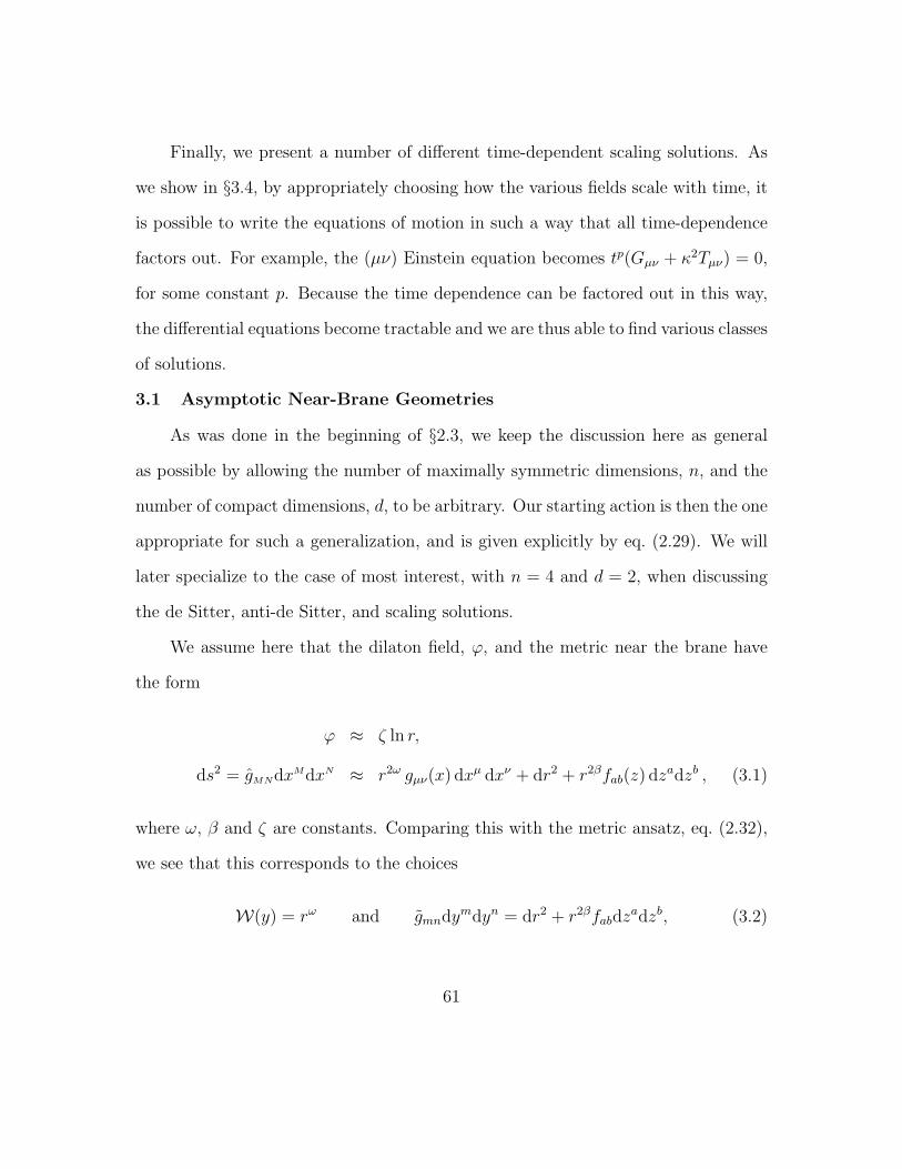
Finally, we present a number of different time-dependent scaling solutions. As

we show in §3.4, by appropriately choosing how the various fields scale with time, it

is possible to write the equations of motion in such a way that all time-dependence

factors out. For example, the (µν) Einstein equation becomes tp(Gµν + κ2Tµν) = 0,

for some constant p. Because the time dependence can be factored out in this way,

the differential equations become tractable and we are thus able to find various classes

of solutions.

3.1 Asymptotic Near-Brane Geometries

As was done in the beginning of §2.3, we keep the discussion here as general

as possible by allowing the number of maximally symmetric dimensions, n, and the

number of compact dimensions, d, to be arbitrary. Our starting action is then the one

appropriate for such a generalization, and is given explicitly by eq. (2.29). We will

later specialize to the case of most interest, with n = 4 and d = 2, when discussing

the de Sitter, anti-de Sitter, and scaling solutions.

We assume here that the dilaton field, ϕ, and the metric near the brane have

the form

ϕ ≈ ζ ln r,

ds2 = gMNdxMdxN ≈ r2ω gµν(x) dxµ dxν + dr2 + r2βfab(z) dzadzb , (3.1)

where ω, β and ζ are constants. Comparing this with the metric ansatz, eq. (2.32),

we see that this corresponds to the choices

W(y) = rω and gmndymdyn = dr2 + r2βfabdzadzb, (3.2)

61

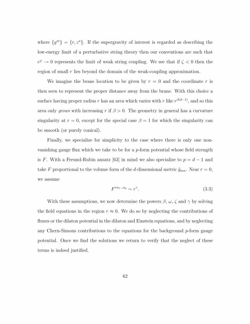
where ym = r, za. If the supergravity of interest is regarded as describing the

low-energy limit of a perturbative string theory then our conventions are such that

eϕ → 0 represents the limit of weak string coupling. We see that if ζ < 0 then the

region of small r lies beyond the domain of the weak-coupling approximation.

We imagine the brane location to be given by r = 0 and the coordinate r is

then seen to represent the proper distance away from the brane. With this choice a

surface having proper radius r has an area which varies with r like rβ(d−1), and so this

area only grows with increasing r if β > 0. The geometry in general has a curvature

singularity at r = 0, except for the special case β = 1 for which the singularity can

be smooth (or purely conical).

Finally, we specialize for simplicity to the case where there is only one non-

vanishing gauge flux which we take to be for a p-form potential whose field strength

is F . With a Freund-Rubin ansatz [63] in mind we also specialize to p = d− 1 and

take F proportional to the volume form of the d-dimensional metric gmn. Near r = 0,

we assume

F ra1...ap ∼ rγ. (3.3)

With these assumptions, we now determine the powers β, ω, ζ and γ by solving

the field equations in the region r ≈ 0. We do so by neglecting the contributions of

fluxes or the dilaton potential in the dilaton and Einstein equations, and by neglecting

any Chern-Simons contributions to the equations for the background p-form gauge

potential. Once we find the solutions we return to verify that the neglect of these

terms is indeed justified.

62

The p-form equation gives the condition

0 = ∂r

(√ge−pϕF rz1...zp

)∼ ∂r

[rωn+β(d−1)−pζ+γ

](3.4)

which leads (when p = d− 1) to the condition γ = (ζ − β)(d− 1)− ωn, and so

F 2 ∼ r2ζ(d−1)−2ωn . (3.5)

Consider next the dilaton equation. We first note that

ϕ =1√g∂M

(√g gMN ∂Nϕ

)∼ ζ[nω + β(d− 1)− 1] r−2. (3.6)

For comparison, the other terms in the dilaton equation of motion depend on r as

follows:

e−pϕF 2 ∼ rζ(d−1)−2ωn and eϕ ∼ rζ . (3.7)

Thus, provided ζ > −2 and ζ(d − 1) − 2ωn > −2 (whose domains of validity we

explore below) all of the terms in the dilaton equation are subdominant to ϕ, and

so may be neglected. The dilaton therefore effectively satisfies ϕ = 0 near r = 0,

and so from eq. (3.6) we see that this requires

nω + β(d− 1) = 1. (3.8)

Next consider the rr-component of the Einstein equation. Given the assumed

asymptotic form for the metric, we calculate

Rrr = [−ωn+ nω2 + (β2 − β)(d− 1)] r−2

= [nω2 + β2(d− 1)− 1] r−2. (3.9)

63

As before, we find that the F 2 term is subdominant if ζ(d − 1) − 2ωn > −2. The

rr-Einstein equation therefore gives the additional constraint

nω2 + β2(d− 1) + ζ2 = 1. (3.10)

Notice that this equation restricts the ranges of ω, β and ζ to be

− 1√n≤ ω ≤ 1√

n, − 1√

d− 1≤ β ≤ 1√

d− 1and − 1 ≤ ζ ≤ 1 . (3.11)

In particular it allows a regular solution (or one having a conical singularity) — i.e.

one having β = 1 — only if d = 2 and ζ = ω = 0.

The Einstein equations in the maximally symmetric dimensions can be similarly

evaluated using the assumed asymptotic form for the metric. The contribution of the

induced n-dimensional curvature tensor contributes to this equation subdominantly

in r, and so is not constrained to leading order. The leading term vanishes as a

consequence of eq. (3.8), and so does not impose any new conditions. Neither do the

Einstein equations in the za directions.

The net summary of the bulk field equations on the parameters β, ω and ζ

is therefore given by the two Kasner-like conditions (3.8) and (3.10). These two

conditions therefore allow a one-parameter family (parameterized, say, by ζ) of so-

lutions in the vicinity of any given singularity. Notice that the symmetry of these

conditions under ζ → −ζ implies that for any given asymptotic solution there is a

new one which can be obtained from the first through the weak-to-strong-coupling

replacement eϕ → e−ϕ.

64

Regarding these singularities as brane sources, the one-parameter set of asymp-

totic bulk configurations presumably corresponds to a one-parameter choice which

is possible for the couplings of the brane to bulk fields. For instance, at the lowest-

derivative level considered here this is plausibly related to the choice of dilaton cou-

pling, such as if the brane action were to take the D-brane form

Sb = −T∫

dnξ√−h eλϕ , (3.12)

where ξµ represent coordinates on the brane world-volume, T is the brane tension,

hµν is the induced metric on the brane. Here the choice for λ (which is a known

function of brane dimension for D-branes) plausibly determines the value of ζ, and

so the value of this parameter is not determined purely from the bulk equations of

motion.

We must now go back to ask whether the Kasner-like conditions (3.8) and (3.10)

are consistent with the requirements ζ > −2 and ζ(d − 1) − 2ωn > −2. The first

inequality clearly follows from the last of eqs. (3.11), and so is automatic for the

solutions of interest. By contrast, constraints (3.8) and (3.10) are not sufficient to

ensure that the second inequality is satisfied, as is seen by using eq. (3.8) to rewrite

it as ζ + 2 β ≥ 0. This is clearly not satisfied by the choices β = 0, ω = 1/n

and ζ = −√

1− 1/n. Since its violation requires either β or ζ to be negative, it

necessarily involves either surfaces, Σβ, whose area does not grow with their radius

(β < 0) or the breakdown of the perturbative supergravity approximation (ζ < 0).

We exclude such solutions in what follows.

65

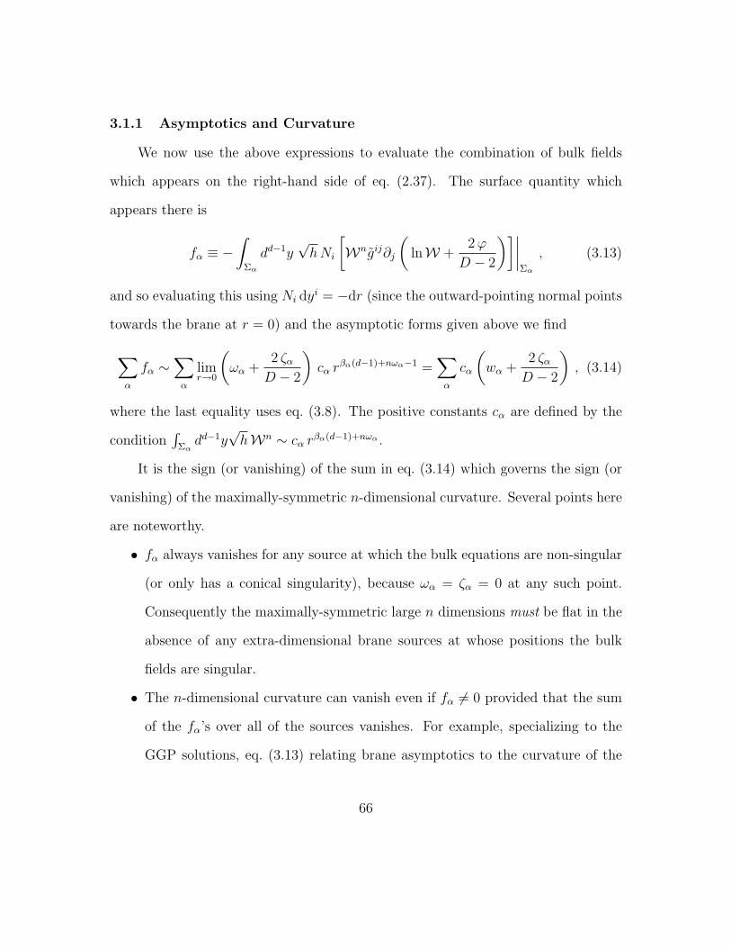
3.1.1 Asymptotics and Curvature

We now use the above expressions to evaluate the combination of bulk fields

which appears on the right-hand side of eq. (2.37). The surface quantity which

appears there is

fα ≡ −∫

Σα

dd−1y√hNi

[Wngij∂j

(lnW +

2ϕ

D − 2

)]∣∣∣∣Σα

, (3.13)

and so evaluating this using Ni dyi = −dr (since the outward-pointing normal points

towards the brane at r = 0) and the asymptotic forms given above we find

∑α

fα ∼∑α

limr→0

(ωα +

2 ζαD − 2

)cα r

βα(d−1)+nωα−1 =∑α

cα

(wα +

2 ζαD − 2

), (3.14)

where the last equality uses eq. (3.8). The positive constants cα are defined by the

condition∫

Σαdd−1y

√hWn ∼ cα r

βα(d−1)+nωα .

It is the sign (or vanishing) of the sum in eq. (3.14) which governs the sign (or

vanishing) of the maximally-symmetric n-dimensional curvature. Several points here

are noteworthy.

• fα always vanishes for any source at which the bulk equations are non-singular

(or only has a conical singularity), because ωα = ζα = 0 at any such point.

Consequently the maximally-symmetric large n dimensions must be flat in the

absence of any extra-dimensional brane sources at whose positions the bulk

fields are singular.

• The n-dimensional curvature can vanish even if fα 6= 0 provided that the sum

of the fα’s over all of the sources vanishes. For example, specializing to the

GGP solutions, eq. (3.13) relating brane asymptotics to the curvature of the

66

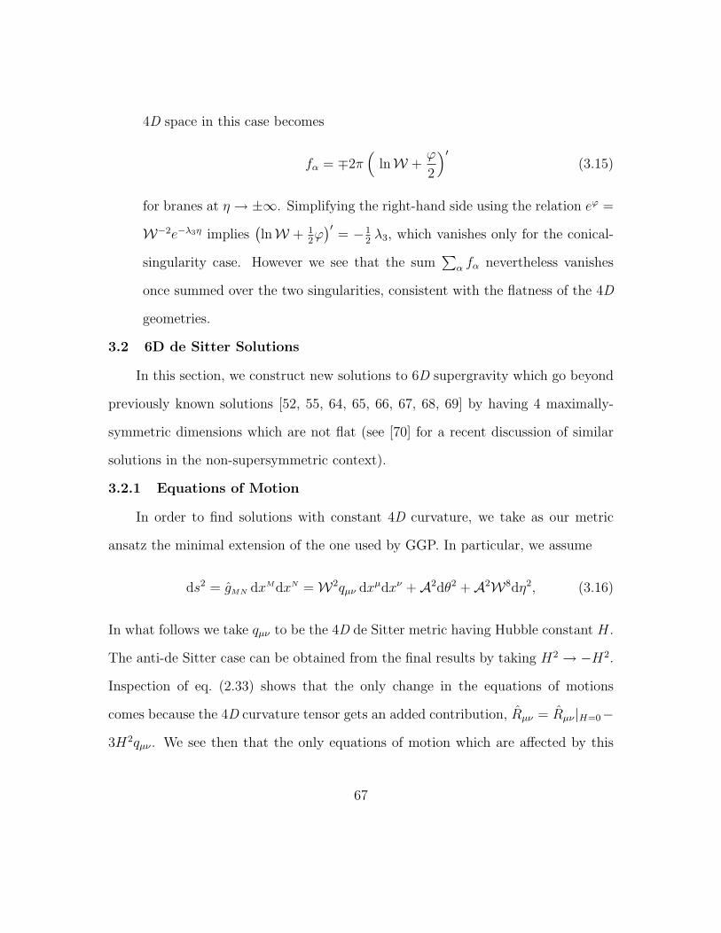
4D space in this case becomes

fα = ∓2π(

lnW +ϕ

2

)′(3.15)

for branes at η → ±∞. Simplifying the right-hand side using the relation eϕ =

W−2e−λ3η implies(lnW + 1

2ϕ)′

= −12λ3, which vanishes only for the conical-

singularity case. However we see that the sum∑

α fα nevertheless vanishes

once summed over the two singularities, consistent with the flatness of the 4D

geometries.

3.2 6D de Sitter Solutions

In this section, we construct new solutions to 6D supergravity which go beyond

previously known solutions [52, 55, 64, 65, 66, 67, 68, 69] by having 4 maximally-

symmetric dimensions which are not flat (see [70] for a recent discussion of similar

solutions in the non-supersymmetric context).

3.2.1 Equations of Motion

In order to find solutions with constant 4D curvature, we take as our metric

ansatz the minimal extension of the one used by GGP. In particular, we assume

ds2 = gMN dxMdxN =W2qµν dxµdxν +A2dθ2 +A2W8dη2, (3.16)

In what follows we take qµν to be the 4D de Sitter metric having Hubble constant H.

The anti-de Sitter case can be obtained from the final results by taking H2 → −H2.

Inspection of eq. (2.33) shows that the only change in the equations of motions

comes because the 4D curvature tensor gets an added contribution, Rµν = Rµν |H=0−

3H2qµν . We see then that the only equations of motion which are affected by this

67

change are the (µν) and (ηη) Einstein equations, which become respectively

W ′′

W− (W ′)2

W2− 3H2A2W6 +

1

2ϕ′′ = 0 (3.17)

6H2A2W6 − 4A′W ′

AW− 6(W ′)2

W2+

1

2(ϕ′)2 +

κ2

2q2A2eϕ − 2g2

1

κ2A2W8eϕ = 0 .

(3.18)

Here, we have used the other equations of motion in order to write the (ηη) equation

in a form involving only first derivatives. The equation of motion for the gauge field

and the dilaton have been given already by eqs. (2.47) and (2.48), respectively.

For numerical purposes we use eqs. (2.47), (2.48) and (3.17) to determine ϕ′′, a′′

and W ′′ as a function of ϕ, a, W , ϕ′, a′ and W ′, and by stepping forward in η generate

a solution as a function of η. By contrast, eq. (3.18) must be read as a constraint

rather than an evolution equation because it contains no second derivatives. The

consistency of this constraint with the evolution equations is guaranteed (as usual)

by general covariance and the Bianchi identities. Evaluating this constraint at the

‘initial’ point, η = η0, gives H in terms of the assumed initial conditions.

3.2.2 Solutions

Recall that the special case of H = 0 corresponds precisely to the solutions

found by GGP. Our goal now is to construct more general solutions to the same

field equations, but with H nonzero, and so for which the maximally-symmetric 4D

geometries are not flat. Although we could do so by directly integrating the field

equations as given above, we instead follow ref. [52] and regard these equations as

68

coming from the following equivalent Lagrangian

L =[(ϕ′)2 − 8(lnW)′(lnA)′ − 12[(lnW)′]2

]N−1

−NA2eϕ(κ2q2 − 4g2

1

κ2W8 + 12H2W6e−ϕ

). (3.19)

This agrees with the form used in [52] when H = 0. We temporarily re-introduce

here the ‘lapse’ function, gηη = N2A2W8, which we choose to reset to unity after

it has been varied in the action. Varying with respect to N gives the constraint

equation (3.18) where we set N = 1 after variation.

The equivalent Lagrangian simplifies if we diagonalize the ‘kinetic’ terms, by

defining the new variables X , Y and Z using1

ϕ =1

2(X −Y − 2Z) , lnW =

1

4(Y −X ) and lnA =

1

4(3X + Y + 2Z) . (3.20)

In terms of these variables the Lagrangian becomes

L = (X ′)2 − (Y ′)2 + (Z ′)2 − κ2q2 e2X +4g2

1

κ2e2Y − 12H2 e2Y+Z . (3.21)

We have setN = 1 but continue to keep in mind its role in determining the constraint.

At this point, it pays to make a further redefinition to absorb all the constants

appearing in the above Lagrangian. The main reason for doing this is that we will

eventually integrate numerically some of the resulting equations of motion. With this

1 In fact, this field redefinition is often used in this thesis as it simplifies theequations of motion considerably.

69

goal in mind, we see that the ‘potential’ terms simplify further if we also redefine

X =1

2ln(κ2q2) + X

Y =1

2ln(4g2

1/κ2) + Y (3.22)

Z = ln |3κ2H2/g21|+ Z

and so

L = (X ′)2 − (Y ′)2 + (Z ′)2 − e2X + e2Y − ε e2Y+Z . (3.23)

where ε = +1 for de Sitter and −1 for anti-de Sitter solutions. We now integrate

the equations of motion obtained from this Lagrangian to obtain explicit solutions

for the extra-dimensional geometries. Since X has the equation of motion

X ′′ + e2X = 0 (3.24)

it decouples from the other variables. Its equation can be directly integrated to give

(X ′)2 + e2X = λ21, (3.25)

and so e−X = λ−11 cosh[λ1(η − ξ1)]. As before, we have chosen to take λ1 > 0. The

remaining two nontrivial equations of motion become in these variables

Y ′′ + e2Y − ε e2Y+Z = 0

Z ′′ +ε

2e2Y+Z = 0 , (3.26)

along with the constraint λ21− (Y ′)2 + (Z ′)2− e2Y + ε e2Y+Z = 0, whose solutions we

obtain numerically below.

70

In terms of these variables the asymptotic behaviour of the solutions assumed in

previous sections near the singularities is linear in η. For example, using eqs. (3.20)

and (3.22) to write X in terms of ϕ and W , and then using the asymptotic forms

given by eqs. (3.1) and (3.2), we see

2X = ϕ+ 2 lnA+ ln(κ2q2

)≈ (ζ± + 2β±) ln r± ≈ ∓(ζ± + 2β±)η, (3.27)

where in the last step we have used that η ≈ ∓ ln r± in the asymptotic region

η → ±∞. Alternatively, from the exact solution for X it is clear that

limη→±∞

X → ∓λ1 η . (3.28)

For the other dependent variables we may similarly write

limη→±∞

Y → ∓λ±2 η,

limη→±∞

Z → ∓λ±3 η, (3.29)

with independent constants λ±i at η → ±∞. By substituting these asymptotic forms

into the differential equations, eqs. (3.26), we immediately obtain the two constraints

λ±2 > 0 and (2λ±2 + λ±3 ) > 0. Note that there is no restriction on the sign of λ±3 .

Finally, the Kasner-like condition in the asymptotic region also imposes the following

constraint on these constants: (λ±2 )2 = λ21 + (λ±3 )2.

The solutions of ref. [52] discussed above satisfy these condition in the special

case where λ±3 = ±|λ3|, and in this case we know the 4D geometries are flat. In

general, however, both the parameters λ±3 are not determined by the one constant

λ3. Using that Z = −ϕ − 2 lnW → ∓λ±3 η and comparing with eq. (3.13), we see

71

Figure 3–1: Typical behaviour of Y as a function of η for de Sitter solutions (ε = +1).The function interpolates between two asymptotically linear regimes. The gradientis always positive as η → −∞ and negative as η → +∞.

Figure 3–2: Typical behaviour of Z as a function of η for de Sitter solutions (ε = +1).The solutions are asymptotically linear with different gradients. For a suitable choiceof initial data the gradient can change sign as in Fig. 3–1.

72

in this case that the sum∑± f± does not vanish, leading to the conclusion that

the corresponding 4D geometries cannot be flat. We have been unable to obtain

analytic solutions to these equations, but there is no obstruction to their integration.

They can be solved numerically leading to numerical profiles such as those given in

Figures 3–1 and 3–2.

3.3 Static Solutions with Broken 4D Lorentz Symmetry

In this section we describe a broad class of static compactifications which are

more general than previous solutions in that they allow 4D Lorentz symmetry to

be broken. When the parameter which controls this breaking is turned off, these

solutions reduce to the GGP solutions discussed in §2.3.2.

3.3.1 Equations of Motion

We start by writing out the field equations for configurations which are (i)

time-independent; (ii) translation and rotation invariant in the 3 noncompact spatial

dimensions; and (iii) are axially symmetric in the extra dimensions. That is, we take

ds2 = −e2w(η) dt2 + e2a(η) δij dxidxj + e2v(η) dη2 + e2b(η)dθ2

Aθ = aθ(η) and eϕ = eϕ(η) , (3.30)

73

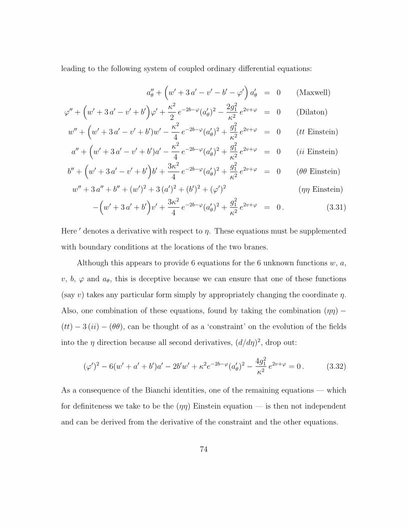
leading to the following system of coupled ordinary differential equations:

a′′θ +(w′ + 3 a′ − v′ − b′ − ϕ′

)a′θ = 0 (Maxwell)

ϕ′′ +(w′ + 3 a′ − v′ + b′

)ϕ′ +

κ2

2e−2b−ϕ(a′θ)

2 − 2g21

κ2e2v+ϕ = 0 (Dilaton)

w′′ +(w′ + 3 a′ − v′ + b′)w′ − κ2

4e−2b−ϕ(a′θ)

2 +g2

1

κ2e2v+ϕ = 0 (tt Einstein)

a′′ +(w′ + 3 a′ − v′ + b′)a′ − κ2

4e−2b−ϕ(a′θ)

2 +g2

1

κ2e2v+ϕ = 0 (ii Einstein)

b′′ +(w′ + 3 a′ − v′ + b′

)b′ +

3κ2

4e−2b−ϕ(a′θ)

2 +g2

1

κ2e2v+ϕ = 0 (θθ Einstein)

w′′ + 3 a′′ + b′′ + (w′)2 + 3 (a′)2 + (b′)2 + (ϕ′)2 (ηη Einstein)

−(w′ + 3 a′ + b′

)v′ +

3κ2

4e−2b−ϕ(a′θ)

2 +g2

1

κ2e2v+ϕ = 0 . (3.31)

Here ′ denotes a derivative with respect to η. These equations must be supplemented

with boundary conditions at the locations of the two branes.

Although this appears to provide 6 equations for the 6 unknown functions w, a,

v, b, ϕ and aθ, this is deceptive because we can ensure that one of these functions

(say v) takes any particular form simply by appropriately changing the coordinate η.

Also, one combination of these equations, found by taking the combination (ηη) −

(tt)− 3 (ii)− (θθ), can be thought of as a ‘constraint’ on the evolution of the fields

into the η direction because all second derivatives, (d/dη)2, drop out:

(ϕ′)2 − 6(w′ + a′ + b′)a′ − 2b′w′ + κ2e−2b−ϕ(a′θ)2 − 4g2

1

κ2e2v+ϕ = 0 . (3.32)

As a consequence of the Bianchi identities, one of the remaining equations — which

for definiteness we take to be the (ηη) Einstein equation — is then not independent

and can be derived from the derivative of the constraint and the other equations.

74

3.3.2 Solutions

Before continuing, we pause to point out that one useful trick for solving these

complicated equations of motion is making a smart choice for the radial coordinate.

Naively, one might think that the Gaussian-Normal gauge choice, v = 1, is best since

that leads to one fewer equation of motion. However, it pays to not commit to a

specific gauge until after examining the equations of motion. In this case, we see

that 4 of the 5 equations of motion can be simplified immensely by the choice

v = w + 3a+ b+ lnN. (3.33)

We will eventually choose the gauge N = 1, but until then the above equation should

be treated simply as a field redefinition, trading v for N . The remaining Maxwell

equation can be integrated exactly, giving

a′θ = qe−(w+3a−v−b−ϕ) = qNe2b+ϕ (3.34)

where in the second equality we have used the field redefinition for v. Plugging this

solution into the equations of motion, we note that the arguments of the exponentials

in these equations are functions of either (2b+ϕ), or (2v+ϕ) = 2(w+ 3a+ b+ϕ/2).

Thus, it will pay to make the redefinitions

X = b+1

2ϕ (3.35)

Y = w + 3a+ b+1

2ϕ. (3.36)

75

Inspection of the equations shows that two other useful choices for redefinitions are

Z = −1

2(w + 3a+ 2ϕ) (3.37)

ξ =1

4(w − a) (3.38)

At this point, it is straightforward to integrate the resulting equations.

Before proceeding, however, we pause to comment that these equations of motion

as well as the constraint equation can be derived from an equivalent Lagrangian, just

as in the case of the de Sitter solutions in §3.2. This Lagrangian is given by

S =

∫dη

[N−1

[(X ′)2 − (Y ′)2 + (Z ′)2 + 12(ξ′)2

]−N

[κ2q2e2X − 4g2

1

κ2e2Y]]

,

(3.39)

where we see now that N plays the role of a Lagrange multiplier and so can be set

to unity after variation. Notice that for ξ′ = 0, this is the same as the equivalent

Lagrangian in §3.2 with H = 0. This should be expected, since from eqs. (3.30) and

(3.38) we see that ξ′ is the quantity which measures 4D Lorentz breaking. Thus, for

ξ′ = 0 these solutions must reduce to the GGP solutions of §2.3.2.

This system can be solved exactly, giving (with N = 1):

e−X =κq

λ1

cosh[λ1 (η − ξ1)] (3.40)

e−Y =2g1

κλ2

cosh[λ2 (η − ξ2)] (3.41)

Z = z0 + λ3 η (3.42)

ξ = ξ0 + λ4 η , (3.43)

76

while integrating the Maxwell equation (3.34) gives

aθ =λ1

q(tanh[λ1(η − ξ1)] + α) (3.44)

The constraint equation amounts to the condition λ22 = λ2

1 + λ23 + 12λ2

4. Note that

it is the integration constant λ4 which controls 4D Lorentz breaking, since λ4 = 0

implies ξ′ = 0. As discussed already, these solutions then reduce to the GGP ones.

Finally, note that we can set two of the parameters ξ1, ξ2, z0, ξ0 to zero by coordinate

rescalings without loss of generality.

3.3.3 Asymptotic Forms

These solutions describe geometries which become singular at η = ±∞, which

are interpreted as being the positions of the 3-branes which source this configuration.

Since it is ultimately the internal structure of the brane (if any) which is responsi-

ble for resolving these singularities, one expects this structure to be related to the

asymptotic limit of the above solutions in the near-brane limit. We therefore pause

here to outline what this asymptotic near-brane behaviour is.

As before, it is useful to adopt Gaussian-Normal coordinates near the brane for

which ds2 = gab dxadxb + dr2, where xa denotes the 5 other coordinates, xa =

xµ, θ = t, xi, θ, with the brane position being described by r = 0. We take the

asymptotic form of the bulk fields in the near-brane limit (r >∼ `) to be generically

given by a power law [1]

ds2 ∼ −[cω(H1r)ω]2 dt2 + [cα(H1r)

α]2 δij dxidxj + dr2 + [cθ(H1r)β−1]2r2dθ2

eϕ ∼ cϕ(H1r)ζ and F rθ ∼ cf (H1r)

γ , (3.45)

77

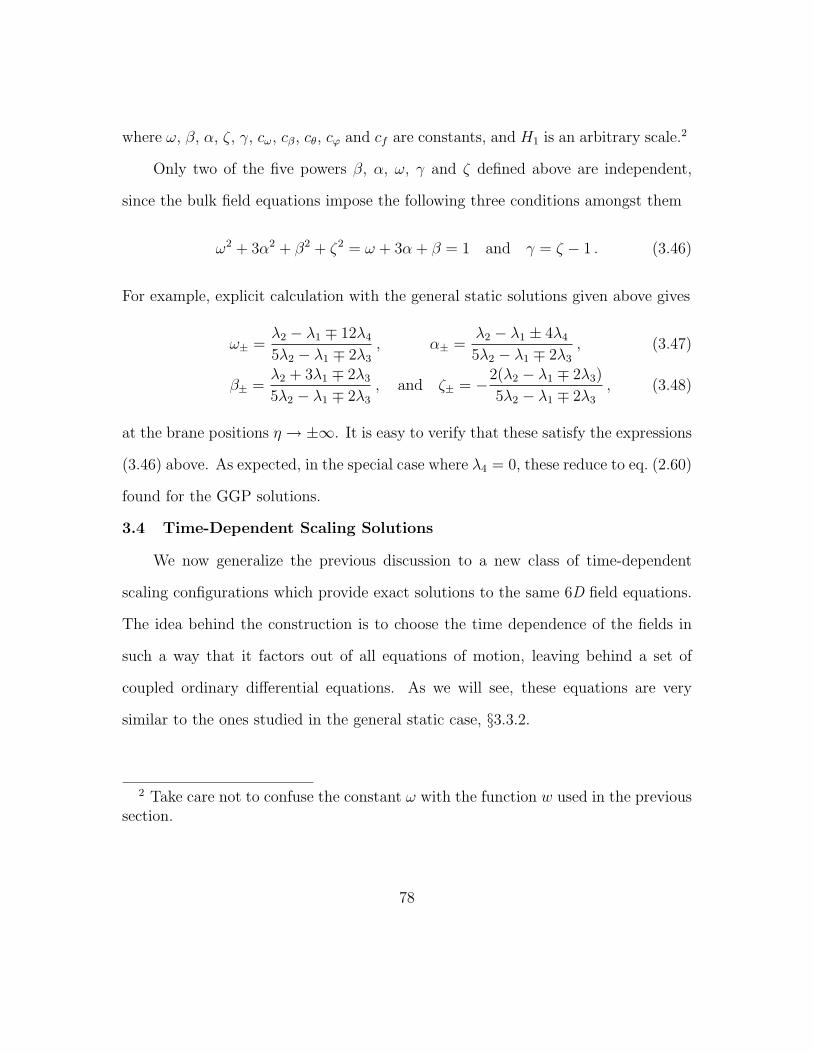
where ω, β, α, ζ, γ, cω, cβ, cθ, cϕ and cf are constants, and H1 is an arbitrary scale.2

Only two of the five powers β, α, ω, γ and ζ defined above are independent,

since the bulk field equations impose the following three conditions amongst them

ω2 + 3α2 + β2 + ζ2 = ω + 3α + β = 1 and γ = ζ − 1 . (3.46)

For example, explicit calculation with the general static solutions given above gives

ω± =λ2 − λ1 ∓ 12λ4

5λ2 − λ1 ∓ 2λ3

, α± =λ2 − λ1 ± 4λ4

5λ2 − λ1 ∓ 2λ3

, (3.47)

β± =λ2 + 3λ1 ∓ 2λ3

5λ2 − λ1 ∓ 2λ3

, and ζ± = −2(λ2 − λ1 ∓ 2λ3)

5λ2 − λ1 ∓ 2λ3

, (3.48)

at the brane positions η → ±∞. It is easy to verify that these satisfy the expressions

(3.46) above. As expected, in the special case where λ4 = 0, these reduce to eq. (2.60)

found for the GGP solutions.

3.4 Time-Dependent Scaling Solutions

We now generalize the previous discussion to a new class of time-dependent

scaling configurations which provide exact solutions to the same 6D field equations.

The idea behind the construction is to choose the time dependence of the fields in

such a way that it factors out of all equations of motion, leaving behind a set of

coupled ordinary differential equations. As we will see, these equations are very

similar to the ones studied in the general static case, §3.3.2.

2 Take care not to confuse the constant ω with the function w used in the previoussection.

78

Before going on to solve the time-dependent solutions, we first pause to demon-

strate how the scaling symmetry discussed earlier can be exploited. Recall that this

symmetry tells us that given any solution to the equations of motion, a new solution

can be obtained through the transformations gMN = eσgMN and ϕ = ϕ − σ, where

σ is a constant. The idea now will be to take σ = σ(x). We know that under this

conformal transformation, the Ricci tensor transforms as3

RMN = RMN −1

2(D − 2)σ;MN −

1

2gMNσ;P

P +1

4(D − 2)(σ;Mσ;N − gMNσ;Pσ

;P ) (3.49)

where a semicolon denotes covariant differentiation with respect to the original met-

ric, gMN , and we have left arbitrary the dimension of spacetime, D. It can also be

shown that

ϕ = e−σ[ϕ−σ +

1

2(D − 2)(ϕ;M − σ;M)σ;M

]. (3.50)

Notice that each of these expressions scales by a specific overall factor of eσ. Scale

invariance now assures us that this will factor out of all equations of motion. For

example, the dilaton equation will be e−σ(ϕ + . . .) = 0, and so we can multiply

both sides by eσ to remove this overall factor.

Now, we specialize to the case σ = σ(t), and take the fieds ϕ and gMN to be

independent of time. Assuming also that the metric is diagonal, we have

ϕ = e−σ[ϕ− gtt(σ + 2σ2)

], (3.51)

3 See, for example, appendix F in [72]

79

where we now specialize to the case D = 6, and we use a dot to denote differentiation

with respect to time. Using this result in the dilaton equation of motion gives

ϕ+κ2

4e−ϕFMNF

MN − 2g21

κ2eϕ − gtt(σ + 2σ2) = 0. (3.52)

Since all fields except σ(t) are assumed to be independent of time, we see that

this is only consistent if (σ + 2σ2) is a constant. The simplest way to satisfy this

constraint is to take σ = Ht. It is easy to check now that with this choice, Rtt = Rtt,

Rij = Rij, and Rti = Rti+12Hgtt∂igtt, where i and j are spatial indices. We can again

use these results in the equations of motion and we find that all time-dependence

disappears. This special choice of time-dependence therefore results in a considerable

simplification.

In the following sections, we focus on the case where all fields depend on time

as well as a single spatial coordinate, η. Choosing the time-dependence of the fields

in a manner similar to above, we see that the equations of motion reduce to a set of

ordinary — as opposed to partial — differential equations.

3.4.1 Equations of Motion

Our ansatz for the metric is a generalization of the static solution which allows

for power law time dependence. In particular, we take

ds2 = (H0t)c[−e2w(η)dt2 + e2a(η) δij dxidxj

]+ (H0t)

c+2[e2v(η)dη2 + e2b(η)dθ2

], (3.53)

where c is an arbitrary dimensionless constant and H0 is a constant having dimension

of inverse time. In some cases it will be natural to take H0 < 0 so that the direction

of increasing time corresponds to t → 0−. Notice that this is a more general time

80

dependence than discussed in the previous section because the large and compact

dimensions scale differently with time. We should expect, however, that this will

reduce to the simpler case in the limit of large c.

The key point to recognize is that with this choice the components of the Ricci

tensor also scale as a simple power of t: Rµν ∝ t−2, Rtη ∝ t−1 and Rmn ∝ t0. Because

of this, and of the scale-invariance of the supergravity equations, it is also possible to

scale the other fields in the problem with t in such a way as to ensure that the field

equations are also proportional to specific powers of t. From the above comments,

we see that we require the following time dependence for the gauge field and the

dilaton:

Aθ = aθ(η) and eφ =eϕ(η)

(H0t)c+2. (3.54)

By virtue of the way the Ricci tensor scales with t, with the above ansatz all

of the field equations reduce to the following set of coupled ordinary differential

equations which govern the η-dependence of the various undetermined functions.

The Maxwell equation is

a′′θ +(w′ + 3 a′ − b′ − v′ − ϕ′

)a′θ = 0 , (3.55)

while the Dilaton equation similarly becomes

ϕ′′ +(w′ + 3 a′ − v′ + b′

)ϕ′ + (c+ 2)(2c+ 1) e−2w+2vH2

0 (3.56)

+κ2

2e−2b−ϕ(a′θ)

2 − 2g21

κ2e2v+ϕ = 0 .

81

The Ricci tensor for this class of metrics is easily computed and leads to the following

components for the Einstein equations. The (tη) component is

(2c+ 1)w′ + 3 a′ + (c+ 2)ϕ′ = 0 , (3.57)

while the (tt) equation is

w′′+(w′+3a′−v′+b′

)w′−κ

2

4e−2b−ϕ(a′θ)

2+g2

1

κ2e2v+ϕ−

(c2 +

5

2c+ 4

)e−2w+2vH2

0 = 0 .

(3.58)

The (θθ) equation is

b′′+(w′+3a′−v′+b′

)b′+

3κ2

4e−2b−ϕ(a′θ)

2 +g2

1

κ2e2v+ϕ− 1

2(c+2)(2c+1)e−2w+2vH2

0 = 0 ,

(3.59)

the (ii) Einstein equation becomes

a′′+(w′+3a′−v′+b′

)a′−κ

2

4e−2b−ϕ(a′θ)

2+g2

1

κ2e2v+ϕ−1

2c (2c+1)e−2w+2vH2

0 = 0 , (3.60)

and finally the (ηη) equation is

w′′ + 3a′′ + b′′ + (w′)2 + 3(a′)2 + (b′)2 + (ϕ′)2 −(w′ + 3a′ + b′

)v′ (3.61)

+3κ2

4e−2b−ϕ(a′θ)

2 +g2

1

κ2e2v+ϕ − 1

2(c+ 2)(2c+ 1)e−2w+2vH2

0 = 0 ,

where ′ = d/dη.

Note that because of the inclusion of time dependence, two components of the

Bianchi identity are nontrivial rather than one. This implies that now two of the

field equations are not independent of the others. Related to this is the existence

in this case of two constraint equations which do not involve d2/dη2, which the

82

Bianchi identities ensure are preserved when evolved using the field equations in

the η direction. These constraints can be taken to be the (tη) Einstein equation,

eq. (3.57), and the combination (ηη)− (tt)− 3(ii)− (θθ):

(ϕ′)2−6(w′+a′+b′)a′−2b′w′+κ2e−2b−ϕ(a′θ)2− 4g2

1

κ2e2v+ϕ+4(c2+c+1)e−2w+2vH2

0 = 0 .

(3.62)

Notice that if we set H0 = 0, all equations except the (tη) Einstein equation are the

same as we found in the static case, §3.3.2. This suggests that we can again simplify

these equations by using the same field redefinitions as in the previous section.

3.4.2 Solutions

Proceeding as before, then, we make the gauge choice v = w + 3a + b (i.e. we

take N = 1 from the start). Then the Maxwell equation integrates as before to give

a′θ = qe2X . (3.63)

while the two constraint equations written in the variables of the previous section

are

0 = 6c ξ′ − (c+ 2)Z ′ (3.64)

0 = (X ′)2 − (Y)2 +4(c2 + c+ 1)

3c2(Z ′)2 + κ2q2e2X

−4g21

κ2e2Y + 4H2

0 (c2 + c+ 1)e2Y−2Z/c. (3.65)

83

The remaining equations of motion simplify to

X ′′ + κ2q2e2X = 0

Y ′′ + 4g21

κ2e2Y − 4H2

0 (c2 + c+ 1) e2Y−2Z/c = 0 (3.66)

Z ′′ − 3cH20 e

2Y−2Z/c = 0.

We note that, as in previous sections, we can obtain these equations of motion, as

well as the constraint equation (3.65), from the equivalent Lagrangian

S =

∫dη

N−1

[(X ′)2 − (Y ′)2 +

4(c2 + c+ 1)

3c2(Z ′)2

]− N

[κ2q2e2X − 4g2

1

κ2e2Y + 4H2

0 (c2 + c+ 1)e2Y−2Z/c]

,(3.67)

where again N plays the role of a Lagrange multiplier.

As before, both x and aθ decouple and have solutions given previously by

eqs. (3.40) and (3.44), respectively. The remaining two equations do not appear

to have closed-form solutions, although they are again straightforward to integrate

numerically, having qualitatively the same form as the de Sitter solutions con-

sidered in §3.2.4 This relation with the de Sitter solutions is not surprising since

these solutions may be obtained as the special case c = −2 of the above scaling

solutions. The asymptotic form of these solutions as η → ±∞ is Y → ∓λ±2 η

and Z → ∓λ±3 η, with λ±2 > 0 and 2λ±2 −(

2c

)λ±3 > 0. The constraint implies

(λ±2 )2 = λ21 + 4(c2 + c+ 1)(λ±3 )2/(3c2).

4 See also [70] for de Sitter solutions in the non-supersymmetric case.

84

3.4.3 Useful Special Cases

There are several special cases of the previous solutions which are of particular

interest.

Connection to 4D scaling solutions

If c = −1 then the metric and dilaton have the time dependence

ds2 =1

tgµν(y) dxµdxν + t gmn(y) dymdyn and eφ =

eϕ

t, (3.68)

which implies in particular that√−g gµν is independent of t.

Such a scaling solution has a simple interpretation in the limit where the extra

dimensions are large enough to justify a description in terms of an appropriate low-

energy 4D effective theory [58]. In the classical limit this theory contains two massless

modes, corresponding to the 4D metric and one combination of the dilaton, φ, and

radius, r, of the extra dimensions (for which r2eφ is fixed) which parameterizes a flat

direction of the 4D scalar potential. The above scaling solution describes a time-

dependent scaling along this flat direction with a fixed metric in the 4D Einstein

frame. (More general choices for c also rescale the Einstein-frame 4D metric.)

Explicit scaling solutions to the field equations of the effective 4D theory de-

scribing these modes are known, many of which are attractor solutions to which a

broad class of initial conditions are drawn [73]. The solutions found here show how

to extend those of the effective 4D theory to see the profiles of the other nonzero KK

modes. Because the 4D solutions are attractors for the 4D field equations, we might

also expect that the same may be true for the higher-dimensional solutions found

here.

85

Pure tension branes

It is known that even for the special case of pure tension branes, maximally-

symmetric solutions to the 6D field equations only exist when the tensions of the two

branes are adjusted relative to one another [51, 52, 53]. One might hope that the

above scaling solutions describe the late time behaviour of the solutions in the case

that the brane tensions are not adjusted in the appropriate way.

We now show that a subset of the solutions found above can indeed describe

this situation. In order to do so we must identify when the asymptotic form of the

solutions near the branes have the pure tension form where a ∼ w, i.e. ξ → 0. Since

the (ηt) constraint implies ξ′ = (c + 2)Z ′/(6c) there are only two circumstances for

which ξ′ → 0 near a brane:

(i) Z ′ → 0 , or (ii) c = −2 . (3.69)

Special case c =∞

Case (i) of (3.69) corresponds to the special case where the geometry near the

brane has a conical singularity, since this always requires Z ′ → 0 in the near-brane

limit. While this is always possible for one brane, in general it is not possible for

both branes since the equation of motion for Z is

Z ′′ − 3cH20 e

2Y−2Z/c = 0, (3.70)

and so |Z ′′| > 0. There is however, one special case for which this can be achieved.

Defining H0 = cH0 such that H0 remains constant (i.e. we take H0 → 0 as c→∞)

and taking the limit c→∞ we recognize that the originally coupled system for Y ,Z

86

decouples,

Y ′′ + 4g21

κ2e2Y − 4H2

0e2Y = Z ′′ = 0. (3.71)

For which the conical solution is

e−Y =2

κλ2

√(g2

1 − κ2H20

)cosh[λ2(η − ξ2)], Z = Z0. (3.72)

As before we can choose Z0 = 0 without loss of generality. Although the metric,

eq. (3.53), appears to be singular in this limit, this is only a consequence of an

inconvenient choice for the time coordinate. If we instead convert to ‘proper’ time,

τ , defined by dτ = (H0t)c/2dt, then τ ∝ t1+c/2 and the metric of eq. (3.53) has a

smooth large-c limit:

ds2 = −e2w(η)dτ 2 +1

4(H0τ)2

[e2a(η) δij dxidxj + e2v(η)dη2 + e2b(η)dθ2

]. (3.73)

We now convert back to ‘conformal’ time, t, using dτ = 12(H0τ) dt, then (H0τ)2 ∝

eH0t, and so

ds2 = eH0t[−e2w(η)dt2 + e2a(η) δij dxidxj + e2v(η)dη2 + e2b(η)dθ2

]. (3.74)

In these same coordinates, we note that the dilaton behaves as as ϕ(t, η) = ϕ(η)−H0t.

Defining σ(t) = H0t, we can write this more suggestively as

ds2 = eσ(t)gMN(η)dxMdxN and ϕ(t, η) = ϕ(η)− σ(t), (3.75)

which we recognize as the solution discussed in the introduction to this section.

As before, we can now determine the singularities of this solution in the limit

η → ±∞. Converting to proper radius dr = ev(η)dη and identifying with the conical

87

deficit form dr2 + (1− δ/2π)2r2 dθ2 we infer the deficit angles(1− δ±

2π

)=

2λ2 e±λ2(ξ1−ξ2)

|q|κ3/2

√g2 − κ2H2

0 . (3.76)

It is clear that by choosing any two of λ2, ξ1, ξ2 and H0 appropriately, we can match

this solution onto two conical branes of arbitrary tensions.

Special case c = −2

Option (ii) of (3.69) makes the choice c = −2, since in this case the (tη) Einstein

equation implies the strong statement that ξ′ = 14(w−a) = 0 everywhere throughout

the bulk. For this special case the 6D geometry is everywhere maximally symmetric

in the noncompact 4 dimensions, taking the form

ds2 = e2w(η)ds2dS4 + e2v(η)dη2 + e2b(η)dθ2 , (3.77)

where dS4 is the 4D de Sitter metric. These are just the de Sitter geometries consid-

ered previously. Notice that there are no de Sitter solutions where both branes are

conical.

3.4.4 Asymptotic Forms

We now re-examine the near-brane behaviour of these scaling solutions in order

to connect their properties to those of the source branes. If we repeat the analysis

of asymptotic forms given earlier for static solutions for the scaling solutions, with

near-brane asymptotic form assumed to be given by eq. (3.53), we find two changes

relative to the static case. The simplest change is simply that the assumed time

dependence implies that the coefficients cw, ca, etc. now depend explicitly on t, with

c2w(t) ∝ c2

a(t) ∝ tc , c2θ(t) ∝ t2+c and c2

φ(t) ∝ t−2−c . (3.78)

88

The second change is to do with the relationship amongst the powers α, β, γ,

ω and ζ which is dictated by the bulk equations. For instance, in the static case

these equations required the powers to be related to one another by the Kasner-like

conditions ω + 3α + β = ω2 + 3α2 + β2 + ζ2 = 1. These conditions also apply for

the scaling solutions, unchanged by c and H0 because the relevant terms in the field

equations are subdominant in powers of r. However, in the scaling case there is also

a new constraint, eq. (3.57), coming from the (tη) Einstein equation, which implies

the following for the asymptotic powers:

(2 c+ 1)ω + 3α + (2 + c) ζ = 0 . (3.79)

3.5 Discussion

Scaling solutions are often attractor solutions towards which general time-dep-

endent configurations tend after the passage of any initial transients. If this is also so

for the 6D supergravity field equations, we would be led to the following attractive

picture. It has long been known [51, 52, 53] that static (and maximally-symmetric,

but curved [1]) solutions can only exist if the properties of the two source branes

are appropriately adjusted relative to one another. But it has been unknown what

happens to the bulk geometry in the generic case where such adjustments are not

made, although it has been suspected that these would produce time-dependent bulk

configurations. Based on the above considerations, in the generic case we expect that

the bulk is indeed time-dependent, and in particular this time-dependence approaches

one of the scaling solutions given here (once transients pass) at late times.

89

CHAPTER 4Perturbative Stability of the GGP Solutions

In the previous chapter we presented a broad class of time-dependent scaling

solutions for 4D compactifications of 6D supergravity. These solutions aid in un-

derstanding the evolution produced by generic brane properties by showing what

the late-time evolution of the system is likely to be for a wide class of initial con-

ditions. The present chapter is aimed at a complementary part of the problem of

time-dependence. Instead of seeking the late-time behaviour towards which the sys-

tem evolves, we here study how small perturbations can initiate the beginnings of

time-dependent behaviour. (See ref. [74] for a description of some of the intermediate

and transient time-dependent phenomena which lies between these two cases.) We

do so by investigating the linear perturbations of a broad class of static solutions to

6D supergravity, in order to see how they respond to arbitrary small perturbations.

In this analysis, we use a Kaluza Klein decomposition which includes both the modes

oscillating in time as well as the zero-mass non-oscillating ones.

Our main result is that these systems are marginally stable for normalizable

perturbations around conical geometries, and for non-singular perturbations around

nonconical ones. (We also examine a class of physically motivated non-regular per-

turbations, for which our stability analysis is inconclusive.) The stability is only

marginal because of the generic scaling property which the 6D supergravity solu-

tions have. (It is the absence of an energy barrier in this marginal direction which

90

allows the development of the scaling solutions of the previous chapter.) We identify

the set of equations which govern the time evolution of the system after all of the

constraints have been used to eliminate some of the field fluctuations, and reproduce

the form found by earlier workers [75].1

We begin in §4.1 and §4.2 with a derivation of the equations governing linearized

perturbations in comoving gauge. §4.3 then solves analytically the linearized equa-

tions in the conical case and identifies the asymptotic behaviour in the more general

non-conical case. We then give in §4.4 several general arguments in favour of the

stability of the modes examined and relate them with the boundary conditions in

§4.3.

4.1 Equations of Motion

We take the following as our metric ansatz

ds2 = e2a ηµν dxµdxν + e2v dη2 + e2bdθ2 (4.1)

and consider these component functions, as well as ϕ and Aθ, to depend only on the

coordinates η and t. (In what follows we sometimes generalize this assumption to

allow dependence on η and xµ.) Denoting differentiation with respect to η and t by

primes and dots, the field equations for these functions then reduce to the following

set of coupled partial differential equations.

1 While our results disagree with earlier versions (as found on the arxiv) of [75],the latest version has corrected an error and so there is no longer a disagreement.

91

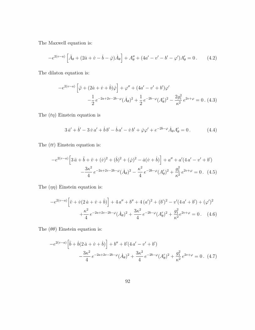
The Maxwell equation is:

−e2(v−a)[Aθ + (2a+ v − b− ϕ)Aθ

]+ A′′θ + (4a′ − v′ − b′ − ϕ′)A′θ = 0 . (4.2)

The dilaton equation is:

−e2(v−a)[ϕ+ (2a+ v + b)ϕ

]+ ϕ′′ + (4a′ − v′ + b′)ϕ′

−1

2e−2a+2v−2b−ϕ(Aθ)

2 +1

2e−2b−ϕ(A′θ)

2 − 2g21

κ2e2v+ϕ = 0 . (4.3)

The (tη) Einstein equation is

3 a′ + b′ − 3 v a′ + b b′ − b a′ − v b′ + ϕϕ′ + e−2b−ϕAθA′θ = 0 . (4.4)

The (tt) Einstein equation is:

−e2(v−a)[3 a+ b+ v + (v)2 + (b)2 + (ϕ)2 − a(v + b)

]+ a′′ + a′(4 a′ − v′ + b′)

−3κ2

4e−2a+2v−2b−ϕ(Aθ)

2 − κ2

4e−2b−ϕ(A′θ)

2 +g2

1

κ2e2v+ϕ = 0 . (4.5)

The (ηη) Einstein equation is:

−e2(v−a)[v + v(2 a+ v + b)

]+ 4 a′′ + b′′ + 4 (a′)2 + (b′)2 − v′(4 a′ + b′) + (ϕ′)2

+κ2

4e−2a+2v−2b−ϕ(Aθ)

2 +3κ2

4e−2b−ϕ(A′θ)

2 +g2

1

κ2e2v+ϕ = 0 . (4.6)

The (θθ) Einstein equation is:

−e2(v−a)[b+ b(2 a+ v + b)

]+ b′′ + b′(4 a′ − v′ + b′)

−3κ2

4e−2a+2v−2b−ϕ(Aθ)

2 +3κ2

4e−2b−ϕ(A′θ)

2 +g2

1

κ2e2v+ϕ = 0 . (4.7)

92

The (ij) Einstein equation is:

−e2(v−a)[a+ a(2 a+ v + b)

]+ a′′ + a′(4 a′ − v′ + b′)

+κ2

4e−2a+2v−2b−ϕ(Aθ)

2 − κ2

4e−2b−ϕ(A′θ)

2 +g2

1

κ2e2v+ϕ = 0 .(4.8)

4.1.1 Maximally Symmetric 4D Compactifications

Since we wish to perturb about the 4D-flat GGP solutions, we briefly recall their

properties here. These solutions may be written

ea =W , ev = AW4 and eb = A , (4.9)

and so the bulk fields become

ds2 = W2(η) ηµν dxµdxν +A2(η)[W8(η) dη2 + dθ2

]Fηθ =

(qA2

W2

)e−λ3η and e−ϕ =W2 eλ3η , (4.10)

where

W4 =

∣∣∣∣κ2qλ2

2g1λ1

∣∣∣∣ cosh[λ1(η − ξ1)]

cosh[λ2(η − ξ2)]

A−4 =

∣∣∣∣2κ2g1 q3

λ31λ2

∣∣∣∣ e−2λ3η cosh3[λ1(η − ξ1)] cosh[λ2(η − ξ2)] , (4.11)

where the field equations imply the constraint λ22 = λ2

1 + λ23.

We also recall the extremely useful change of variables introduced in §3.2,

ϕ =1

2(X − Y − 2Z) , lnW =

1

4(Y − X ) and lnA =

1

4(3X + Y + 2Z) , (4.12)

93

and so

e−X = e−ϕ/2A−1 =

∣∣∣∣κqλ1

∣∣∣∣ cosh [λ1(η − ξ1)] (4.13)

e−Y = e−ϕ/2A−1W−4 =

∣∣∣∣ 2g1

κλ2

∣∣∣∣ cosh [λ2(η − ξ2)] (4.14)

e−Z = eϕW2 = e−λ3η . (4.15)

It is straightforward to check that these are related by the Hamiltonian constraint

(for evolution in the η direction):

−4g21

κ2e2Y + κ2q2e2X + X ′2 − Y ′2 + Z ′2 = 0 . (4.16)

4.2 Linearization

In this section we set up the equations which govern axially-symmetric pertur-

bations about the solutions described above which transform as scalars in 4D. The

restriction to axially symmetric perturbations does not limit the ensuing stability

analysis because the most unstable modes are generally the most symmetric, since

any angular dependence contributes positively to the corresponding Kaluza-Klein

mass.

4.2.1 Symmetries and Gauge Choices

The most general 4D scalar perturbations have the form

ds2 = e2a[ηµν +M, µν

]dxµdxν + 2Nm,µ dxµdym + gmn dymdyn

B = Bµν dxµ ∧ dxν + 2Bm,µ dxµ ∧ dym +Bmn dym ∧ dyn

and A = Ω,µ dxµ + Am dym , (4.17)

94

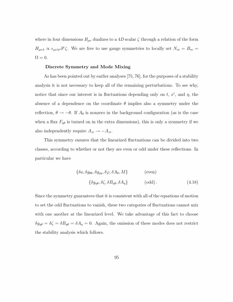
where in four dimensions Bµν dualizes to a 4D scalar ζ through a relation of the form

Hµνλ ∝ εµνλr∂rζ. We are free to use gauge symmetries to locally set Nm = Bm =

Ω = 0.

Discrete Symmetry and Mode Mixing

As has been pointed out by earlier analyses [75, 76], for the purposes of a stability

analysis it is not necessary to keep all of the remaining perturbations. To see why,

notice that since our interest is in fluctuations depending only on t, xi, and η, the

absence of a dependence on the coordinate θ implies also a symmetry under the

reflection, θ → −θ. If Aθ is nonzero in the background configuration (as is the case

when a flux Fηθ is turned on in the extra dimensions), this is only a symmetry if we

also independently require AM → −AM .

This symmetry ensures that the linearized fluctuations can be divided into two

classes, according to whether or not they are even or odd under these reflections. In

particular we have

δa, δgθθ, δgηη, δϕ, δAθ,M (even)

δgηθ, δζ, δBηθ, δAη (odd) . (4.18)

Since the symmetry guarantees that it is consistent with all of the equations of motion

to set the odd fluctuations to vanish, these two categories of fluctuations cannot mix

with one another at the linearized level. We take advantage of this fact to choose

δgηθ = δζ = δBηθ = δAη = 0. Again, the omission of these modes does not restrict

the stability analysis which follows.

95

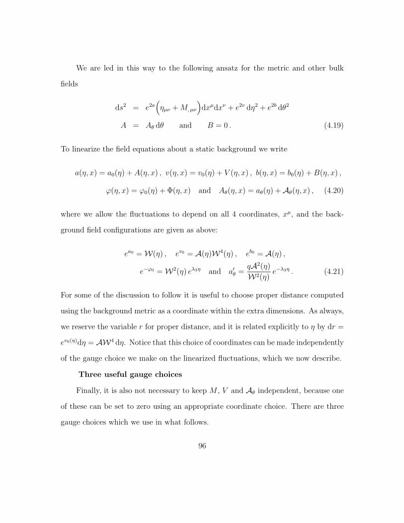
We are led in this way to the following ansatz for the metric and other bulk

fields

ds2 = e2a(ηµν +M, µν

)dxµdxν + e2v dη2 + e2b dθ2

A = Aθ dθ and B = 0 . (4.19)

To linearize the field equations about a static background we write

a(η, x) = a0(η) + A(η, x) , v(η, x) = v0(η) + V (η, x) , b(η, x) = b0(η) +B(η, x) ,

ϕ(η, x) = ϕ0(η) + Φ(η, x) and Aθ(η, x) = aθ(η) +Aθ(η, x) , (4.20)

where we allow the fluctuations to depend on all 4 coordinates, xµ, and the back-

ground field configurations are given as above:

ea0 =W(η) , ev0 = A(η)W4(η) , eb0 = A(η) ,

e−ϕ0 =W2(η) eλ3η and a′θ =qA2(η)

W2(η)e−λ3η . (4.21)

For some of the discussion to follow it is useful to choose proper distance computed

using the background metric as a coordinate within the extra dimensions. As always,

we reserve the variable r for proper distance, and it is related explicitly to η by dr =

ev0(η)dη = AW4 dη. Notice that this choice of coordinates can be made independently

of the gauge choice we make on the linearized fluctuations, which we now describe.

Three useful gauge choices

Finally, it is also not necessary to keep M , V and Aθ independent, because one

of these can be set to zero using an appropriate coordinate choice. There are three

gauge choices which we use in what follows.

96

• Comoving (c) gauge: defined by the condition A(c)θ = 0, leading to

ds2 = e2a0e2A(c)

ηµνdxµdxν +e2v0e2V (c)

dη2 +e2b0e2B(c)

dθ2 +2N,µ dηdxµ , (4.22)

together with A = aθdθ and ϕ = ϕ0 + Φ(c). Notice that this gauge does not fall

completely into the ansatz of eq. (4.1), because the coordinate transformation

required to get to the form (4.1) does not preserve the condition δAθ = 0.

This is the origin of the new metric variable, δgηµ, in the above expression.

Notice also that we have used the gauge freedom to set M = 0. (For counting

purposes, we see that we have removed one degree of freedom, Aθ, while N

simply replaces the degree of freedom M .)

• Gaussian Normal (GN) gauge: defined by V (GN) = 0, and so:

ds2 = e2a0

(e2A(GN)

ηµν +M (GN),µν

)dxµdxν + e2b0e2B(GN)

dθ2 + dr2 , (4.23)

together with ϕ = ϕ0 + Φ(GN) and Aθ = aθ +A(GN)θ . It is obviously convenient

also to use background-metric proper distance, r, defined via dr = ev0dη.

• Longitudinal (l) gauge: defined by M = 0 and so

ds2 = e2a0e2A(l)

ηµνdxµdxν + e2b0e2B(l)

dθ2 + e2V (l)

dr2, (4.24)

together with ϕ = ϕ0 + Φ(l) and Aθ = aθ +A(l)θ . Notice that we again choose

to use background-metric proper distance, r, as the radial coordinate.

Which of these gauges is most convenient depends on the goal of the calculation.

Comoving gauge is physically intuitive (since one follows perturbations along hy-

persurfaces of constant Aθ), and has the enormous benefit that the field equations

97

completely decouple in this gauge, making the linearization analysis much easier.

Longitudinal gauge is convenient for making contact with earlier calculations in the

literature, since this is the gauge which has often been used. Finally, GN gauge is

useful for analyzing the boundary conditions which fluctuations must satisfy near

the source branes.

It is clearly useful to be able to transform between expressions obtained in these

three gauges, so we next briefly summarize the main formulae which are required.

Under the coordinate transformation xM → xM + ξM , where ξµ = ∂µε and ξr = ε, we

have that to linear order the line element transforms as

ds2 → e2a0

[e2(A+ε ∂ra0)ηµν + ∂µ∂ν(M + 2ε)

]dxµdxν + 2∂µ

[e2a0∂rε+ ε

]drdxµ

+e2(V+∂rε)dr2 + e2b0[e2(B+ε ∂rb0)

]dθ2, (4.25)

while the gauge field and dilaton transform according to

Aθ → Aθ + ε ∂raθ (4.26)

Φ → Φ + ε ∂rϕ0 . (4.27)

Note that in these expressions we choose to use the radial coordinate r as opposed

to η. From these transformations, it is straightforward to move between the various

gauges.

To change from longitudinal to comoving gauge requires the transformation

xM(l) = xM(c) + ξM , with ξM = ε δMr so that r(l) = r(c) + ε, with ε = −A(l)θ /∂raθ required

to ensure A(c)θ = 0 while ε = 0 is chosen to ensure that M (c) = M (l) = 0. This implies

that the various fields in longitudinal gauge are related to the ones in comoving gauge

98

by:

A(c) = A(l) + ε ∂ra0 , B(c) = B(l) + ε ∂rb0 , V (c) = V (l) + ∂rε , (4.28)

N (c) = e4a0+b0ε , Φ(c) = Φ(l) + ε∂rϕ0 .

Similarly, to go from comoving to GN gauge, we perform the transformations

r(c) = r(GN) + ε with ∂rε = −V (c) chosen to ensure V (GN) = 0. The further trans-

formation, xµ(c) = xµ(GN) + ∂µε, with ∂rε = −e−(6a0+b0)N (c) − e−2a0ε is also required

in order to ensure the vanishing of N (GN). Quantities in comoving gauge are then

related to those in GN gauge by

A(GN) = A(c) + ε∂ra0 , M (GN) = 2ε, B(GN) = B(c) + ε∂rb0

Φ(GN) = Φ(c) + ε∂rϕ0, A(GN)θ = ε∂raθ. (4.29)

4.2.2 Linearized Equations in Comoving Gauge

We now work out the perturbed equations in comoving gauge, since in this

gauge we are able to decouple the fluctuations even when perturbing about non-

conical background solutions. Note that the equations of motion given in §4.1 were

in longitudinal gauge, so we could proceed by linearizing these equations and then

using the results of the previous section in order to transform to the desired comoving

gauge. However, it turns out to be easier to derive from scratch the equations of

motion using the metric ansatz appropriate for comoving gauge, eq. (4.22).

In the following, we use the coordinate η with the derivative d/dη denoted by

primes, and we allow to the perturbations to depend on all xµ as well as on η. We

99

adopt a notation for the perturbations where A(c) = −Ψ/2 and V (c) = ξ/2, and so

ds2 = e(Y−X )/2e−Ψ ηµν dxµdxν + e(3X+Y+2Z)/2[e2(Y−X )eξ dη2 + e2B dθ2

]+ 2N,µdη dxµ ,

(4.30)

while eϕ = e(X−Y−2Z)/2eΦ and Fηθ = a′θ = qe2X . In terms of these variables, and

Fourier transforming with respect to time and space2 so = ηµν∂µ∂ν = ω2, the

Maxwell equation is

2ω2e(X−Y)/2N + 2B′ + 2Φ′ + ξ′ + 4Ψ′ = 0 ; (4.31)

the dilaton equation is

Φ′′ + ω2e2Y+ZΦ− 1

2

(κ2q2e2X +

4g2

κ2e2Y)

Φ (4.32)

= ϕ′0

(1

2ξ′ + 2Ψ′ −B′ + ω2e(X−Y)/2N

)+

2g21

κ2e2Yξ + κ2q2e2XB ;

the (µη) Einstein equation is

∂µ

[2(2X ′ + Z ′)B − (2Y ′ + Z ′)ξ + 4ϕ′0Φ + 4B′ − 6Ψ′

]= 0 ; (4.33)

while the other off-diagonal term in the Einstein equation (µ 6= ν) is

∂µ∂ν

[e

12

(X−5Y−2Z) [2N ′ + (X ′ − Y ′)N ]− 2B − ξ + 2Ψ]

= 0. (4.34)

2 We emphasize that ω is the mass of the corresponding Kaluza-Klein mode andshould be understood as the eigenvalue of the operator . In this analysis, we donot make the assumption that the modes have a specific time-oscillatory behaviorof the form eik0t. Thus this analysis includes both time-oscillating modes, and non-oscillating ones which correspond to zero-mass Kaluza Klein modes.

100

A combination of the (ηη) Einstein equation, the dilaton equation of motion and the

trace of the Einstein equation which involves only first derivatives with respect to η

is

ω2

2e(X−Y)/2(2Y ′ + Z ′)N − 2g2

1

κ2e2Yξ +

3ω2

2e2Y+ZΨ (4.35)

+(2Y ′ + Z ′)Ψ′ − 1

2

(κ2q2e2X +

4g21

κ2e2Y)

Φ

+ϕ′0Φ′ − κ2q2e2XB − ω2e2Y+ZB + (X ′ − Y ′)B′ = 0 .

The (θθ) Einstein equation is similarly

(2B′′ + Φ′′) + ω2e2Y+Z(2B + Φ)− 2κ2q2e2X (2B + Φ) + 2X ′B′

= X ′(4Ψ′ + ξ′ + 2ω2e(X−Y)/2N

), (4.36)

and finally, tracing the (µµ) Einstein equations gives

(Φ′′ + ω2e2Y+ZΦ

)−(Ψ′′ + ω2e2Y+ZΨ− 2Z ′Ψ′

)= Z ′

(B′ − 1

2ξ′ − ω2e(X−Y)/2N

). (4.37)

We have here a set of seven equations for five variables (ξ, N , Ψ, B and Φ). Two

of these equations appear as constraints and can be used to fix the lapse and shift

functions: using the (µη) equation (4.33) and the (ηη) equation (4.35), we can express

both ξ and ω2N in terms of the three remaining variables Ψ, B and Φ, leading to

five remaining equations for three variables. However these remaining equations are

not independent since the Bianchi identities ensure that two of them are redundant.

One can be expressed as a linear combination of the others, whilst the derivative of

101

the Maxwell equation (4.31) is simply the derivative of (4.33) and a combination of

the other equations.

We arrive in this way with three equations for three unknowns, which can be

written as

B′′ + ω2e2Y+ZB +1

4

(6X ′ + 2Y ′ + 4Z ′ + 16 g2

1

κ2

e2Y

2Y ′ + Z ′

)B′

+1

8

(−12κ2q2e2X +

16 g21

κ2e2Y 2X ′ + Z ′

2Y ′ + Z ′

)B +

1

4(3X ′ + Y ′ + 2Z ′) Φ′ (4.38)

+1

16

(−12κ2q2e2X +

16 g21

κ2e2Y 2X ′ − 3Z ′

2Y ′ + Z ′

)Φ− 6 g2

1

κ2

e2Y

2Y ′ + Z ′Ψ′ = 0 ,

Ψ′′ + ω2e2Y+ZΨ +12 g2

1

κ2

e2Y

(2Y ′ + Z ′)Ψ′ (4.39)

+1

2(X ′ − Y ′) (Φ′ + 2B′)− 8 g2

1

κ2

e2Y

2Y ′ + Z ′B′ − κ2q2

2e2X (Φ + 2B)

−2 g21

κ2

e2Y

2Y ′ + Z ′[(2X ′ − 3Z ′)Φ + 2(2X ′ + Z ′)B] = 0 ,

and

Φ′′ + ω2e2Y+ZΦ + ϕ′0(Φ′ + 2B′) +4 g2

1

κ2

e2Y

2Y ′ + Z ′(3Ψ′ − 2B′) (4.40)

−κ2q2

2e2X (Φ + 2B)− 2 g2

1

κ2

e2Y

2Y ′ + Z ′[(2X ′ − 3Z ′)Φ + 2(2X ′ + Z ′)B] = 0 .

102

These equations dramatically simplify once the change of variables (Φ, B,Ψ)→

(f, χ, ψ) is performed, with3

Φ =2Uκq

e−Xf − 2B

B =V√3U

χ− 1

2Ψ +

2U2 + X ′Z ′

2κq Ue−Xf (4.41)

Ψ =2Y ′ + Z ′

4Vψ +

2U2 − 3Y ′Z ′

4√

3UVχ+U2 −X ′Y ′

2κq Ue−Xf ,

where use of the background field equations shows that the nominally field-dependent

quantities U and V are really both constants:

U2 ≡ X ′2 + κ2q2e2X = λ21

V2 ≡ X ′2 + κ2q2e2X +3

4Z ′2 = λ2

1 +3

4λ2

3 . (4.42)

Notice that for conical backgrounds U = V = λ1. In terms of these new variables the

three field equations — eqs. (4.38), (4.39) and (4.40) — take the remarkably simple,

decoupled form

χ′′ + ω2e2Y+Zχ = 0 (4.43)

f ′′ + ω2e2Y+Zf − U2f = 0 (4.44)

ψ′′ + ω2e2Y+Zψ − 32 g21 V2e2Y

κ2 (2Y ′ + Z ′)2 ψ = 0 . (4.45)

Because these equations decouple from one another each can be solved sepa-

rately, and presents no problem for numerical analysis. Exact solutions are also

3 Take care not to confuse χ and X !

103

available in the case of backgrounds having conical singularities (including but not

restricted to the rugby-ball geometries), as shall be described in detail in later sec-

tions. It is noteworthy for later purposes that the decoupled equations (4.43 – 4.45)

are independent of the background field X (and hence also of the parameter ξ1). This

implies, for example, that the linearized equations of motion for the variables χ, f ,

and ψ are identical for a general conical background geometry (for which Z ′ = 0) and

a rugby-ball geometry (for which Z ′ = 0 and X ′ = Y ′). However once the solutions

are inserted into the expressions for the metric fluctuations using relations (4.41),

the results do depend on X and so the full fluctuations ‘know’ about the complete

background geometry.

4.3 Properties of Solutions

Up to this point there has been no restriction on the form of the background

geometry. In this section we specialize to special conical backgrounds for which it is

possible to solve the above linearized equations in closed form. We then return to

the more general non-conical geometry in order to discuss the asymptotic behaviour

of the solutions in the near-brane limit. The section closes with an outline of how

this asymptotic form is related to the physical properties of the branes which source

the bulk geometries.

4.3.1 Analytic Solutions for General Conical Backgrounds

We now concentrate on the behaviour of the perturbations to solutions having

only conical singularities, which are defined by the condition λ3 = 0 (and so Z ′ = 0).

Performing the change of variable z = tanh [λ2 (η − ξ2)], the perturbation equations

104

become

d2χ

dz2−(

2z

1− z2

)dχ

dz+

(µ2

1− z2

)χ = 0 (4.46)

d2ψ

dz2−(

2z

1− z2

)dψ

dz+

(1

1− z2

)(µ2 − 2

z2

)ψ = 0 (4.47)

d2f

dz2−(

2z

1− z2

)df

dz+

(1

1− z2

)(µ2 − 1

1− z2

)f = 0, (4.48)

with µ2 = ω2κ2/4g21, and ω is the 4D mode mass. Notice that these equations are

symmetric under z → −z, which corresponds to reflections of η around η = ξ2. The

reason for this symmetry is clear in the special case of the rugby-ball solutions (for

which ξ1 = ξ2), since it then corresponds to reflections of the spherical geometry

about its equator. In the more general warped conical geometries this symmetry

instead follows from the above-mentioned circumstance that the equations are com-

pletely independent of ξ1, and so take the same form for general conical geometries

as they do for the rugby ball.

Defining ν = 12

[−1 +

√1 + 4µ2

]— or equivalently writing µ2 = ν(ν + 1) —

the solutions to these equations become

χ = C1 Pν(z) + C2 ReQν(z) (4.49)

= C1F

[−ν, 1 + ν; 1;

1

2(1− z)

]+C2

√π

Γ(ν + 1)

Γ(ν + 32)

Re1

(2z)ν+1F

[1

2(1 + ν), 1 +

ν

2; ν +

3

2; z−2

]ψ = C3 z

−1F

[−1

2(1 + ν),

ν

2;−1

2; z2

]+ C4 z

2F

[1− ν

2,1

2(3 + ν) ;

5

2; z2

](4.50)

f =1√

1− z2

(C5 F

[ν

2,−1

2(1 + ν);

1

2; z2

]+ C6 z F

[1

2(1 + ν),−ν

2;3

2; z2

])(4.51)

105

where the Ci, i = 1, .., 6 are integration constants and F [a, b; c; z] is the hypergeo-

metric function. Neglecting the overall normalization of all three modes, we see that

the above expressions provide a 9-parameter family of solutions. Notice also that

these solutions can be decomposed into symmetric and anti-symmetric combinations

under the symmetry z → −z, and this is already explicit for the functions ψ and f .

We see that the mode energies satisfy

ω2 =ν(ν + 1)

r20

, (4.52)

with 1/r0 = 2g1/κ, and so the spectrum depends on the values which are allowed

for the parameter ν. Notice that for real ν we have ω2 ≥ 0 except for the interval

−1 < ν < 0. As usual, the values which are allowed for ν are related to the behaviour

which is demanded of the solutions at the boundaries, which in the present instance

corresponds to the near-brane limits z → ±1. For this reason we next explore the

asymptotic form taken by the solutions in the near-brane limit.

4.3.2 Asymptotic Forms

We next examine three aspects of the near-brane limit. In this section we first

explore the asymptotic forms taken by the solutions just constructed for fluctua-

tions about backgrounds having only conical singularities. We then see how these

asymptotic forms generalize to the broader situation where the background has more

generic singularities. A preliminary connection is drawn in the next section between

this asymptotic behaviour and the properties of the source branes.

106

Conical backgrounds

The asymptotic form of the solutions found above near the brane positions at

z = ±1 may be found by using the properties of the Hypergeometric functions given

in appendix B. This shows that for generic ν, χ and ψ diverge logarithmically as one

approaches the branes, whereas f generically diverges as (1− z2)−1/2 ∼ cosh[λ2(η −

ξ2)] ∼ r−1.

As usual, less singular asymptotic behaviour can be possible for those ν for

which the hypergeometric series terminates, which for F [a, b; c; z] occurs when either

a or b is a negative integer (or zero). Inspection of the explicit solutions then shows

that termination can happen when ν is quantized to be a non-negative integer: ν =

` = 0, 1, 2, . . . . Notice that the resulting quantization of KK mass, from eq. (4.52),

implies in this case ω2 ≥ 0.

For ν = ` one — but not both — of the two Hypergeometric functions appearing

for each of χ, ψ and f terminates, allowing a less singular near-brane limit to be ob-

tained through an appropriate choice for the integration constants Ci. For instance,

if we require — as we shall argue on the grounds of normalizability below — that all

fluctuations must be less singular than (1 − z2)−1/2, then this is possible for f only

if ν = ` and one of C5 or C6 vanishes (which one depends on whether ` is even or

107

odd).4 Once this has been done the functions χ and ψ can still diverge logarithmi-

cally as z → ±1, leaving a 4-parameter family of potentially logarithmically singular

solutions (up to overall normalization).

Completely regular solutions are also possible when ν = `, provided that one of

C1 or C2 and one of C3 or C4 also vanishes. For instance, χ is regular everywhere

if ν = ` and C2 = 0 since in this case the solution P` degenerates to the Legendre

polynomials. This leaves a 2-parameter family of non-singular solutions (up to overall

normalization).

Non-conical backgrounds

Although it is difficult to find explicit solutions in the generic case where the

background has non-conical singularities, it is possible to use the linearized equations

to estimate the asymptotic behaviour of the mode functions as η → ±∞ (or z → ±1).

Repeating the steps which led to the equations of the previous section for this more

general case, we instead find

d2χ

dz2−(

2z

1− z2

)dχ

dz+

µ2

(1− z2)

(1 + z

1− z

)δλχ = 0 (4.53)

d2ψ

dz2−(

2z

1− z2

)dψ

dz+

(1

1− z2

)[µ2

(1 + z

1− z

)δλ− 2 (1− δλ2)

z2

]ψ = 0 (4.54)

d2f

dz2−(

2z

1− z2

)df

dz+

(1

1− z2

)[µ2

(1 + z

1− z

)δλ− 1− 4δλ2

1− z2

]f = 0, (4.55)

with µ2 = µ2 eλ3ξ2 and δλ = λ3/2λ2.

4 We give explicit expressions for some of the lowest of these non-singular modesfor ψ and f in appendix A for longitudinal gauge.

108

Since |δλ| < 1/2 the term in eq. (4.53) which is proportional to χ remains

subdominant compared to the terms in (1− z2)−1

dχ/dz and d2χ/dz2, such that

the asymptotic behaviour of χ still remains logarithmic near the brane. Similar

arguments show that ψ and f also keep the same asymptotic behaviour as in the

conical case.

Normalizability

A restriction on the asymptotic forms follows from the condition that the mode

functions be normalizable, as we now explore. As we show in detail in the next

section, the equations of motion for each of the decoupled modes can be derived

from a reduced action, eq. (4.71). In this action all modes, u, have the same kinetic

term, e2Y+Zuu, where e2Y+Z = A2W6, and so the definition of the inner product

can be taken to be the same for all three of χ, ψ, and f , having the form:

〈u, v〉 =i

2

∫Σ

d3x dθ dηA2W6 (u∂tv∗ − u∗∂tv) ,

for any two modes u and v. Here Σ denotes a surface of constant t. The norm of a

mode is therefore defined by

〈u, u〉 = ω

∫Σ

d3x dθ dηA2W6uu∗ = ω

∫Σ

d3x dθ drAW2uu∗, (4.56)

where we use dr/dη = AW4 and ∂tu = −iωu.

Our interest is in the conditions placed on the asymptotic behaviour of linearized

modes by the convergence of these integrals. We take the usual ansatz for the

109

asymptotic form of the metric and fields, namely

ds2 ∼ [ca(Hr)α]2 ηµν dxµdxν + dr2 + [cθ(Hr)

β]2dθ2

eϕ ∼ cφ(Hr)ζ and F ρθ ∼ cf (Hr)γ . (4.57)

Using a subscript zero to denote background quantities, we have AW2 ∝ rβ0+2α0 ∝

r1−2α0 in the near-brane limit (r → 0). In order to be normalizable, modes should

therefore vary as u ∝ rυ with power υ > −1 + α0 as r → 0. In particular, for a

conical background with α0 = 0 and β0 = 1, modes must diverge less rapidly than

1/r near both branes.

4.3.3 Boundary Conditions and Brane Properties

The above considerations show that the stability of the linearized fluctuations

is related to the behaviour of the modes as they approach the branes. In this section

we briefly explore to what extent the properties of the linearized solutions capture

what we know about the asymptotic properties of the exact solutions. Exploring this

connection also allows us to make some contact between the conditions for stability

and the physical properties of the branes which source the bulk field configurations,

through considerations along the lines of those given in refs. [2, 53, 71].

Asymptotics in GN gauge

Recall for these purposes that on general grounds the various bulk fields are

known (in GN gauge) to approach the branes through a power-law form given by

eqs. (3.1). In principle there are two cases to consider, depending on whether or

not the background and perturbed fields share the same powers in these asymp-

totic expressions. That is, if we imagine that the background and perturbed metric

110

components, ea0 and ea = ea0eA, satisfy

ea0 → ca0(Hr)α0 and ea → ca(Hr)α , (4.58)

near r = 0, then we see that the fluctuation field, A, must satisfy

A→ (α− α0) ln(Hr) + ln

(caca0

)+ · · · , (4.59)

in the same limit. Similar expressions also hold for the fields B, V , and Φ.

Since the Maxwell field strength varies as Frθ ∝ rγ+2β ∝ rζ+2β−1 the same

argument has slightly different implications for Aθ, since aθ ∝ rζ0+2β0 and Aθ =

aθ + Aθ ∝ rζ+2β. (Notice that this gives the expected results Frθ ∝ r and Aθ ∝ r2

in the conical case, for which β = 1 and ζ = 0.) In this case we have Aθ ∝ rζ+2β if

ζ + 2β < ζ0 + 2β0, because the small-r behaviour of Aθ dominates that of aθ. Things

are different if ζ + 2β > ζ0 + 2β0, however, since in this case aθ dominates Aθ, and

in order to achieve this Aθ must contain a piece which varies in the same way and

cancels the contribution of aθ as r → 0. As a consequence in this case Aθ ∝ rζ0+2β0

for small r.

How singular this is depends on the allowed range of ζ + 2β. Notice that in

general the constraints 4α + β = 4α2 + β2 + ζ2 = 1 require 54β2 − 1

2β + ζ2 = 3

4.

Solving this equation for ζ, the sum ζ + 2β is thus minimal (‘−’ sign) and maximal

(‘+’ sign) for β = 15∓ 16

5√

21, and ζ = ∓ 2√

21, so that the sum is in the range −1.433 '

25(1 −

√21) ≤ ζ + 2β ≤ 2

5(1 +

√21) ' 2.233. We see that perturbations to Aθ can

become quite singular. In the particular case of conical singularities ζ = 0 and β = 1

and so ζ + 2β = 2, leading to smooth behaviour near the branes.

111

We see from the above that the perturbations need not be smooth at the brane

positions, but that in GN gauge the metric perturbations can at worst diverge loga-

rithmically in the near-brane limit. (Perturbations to the Maxwell field can be more

singular than logarithmic, but only if ζ and β are sufficiently negative.) Since the

arguments of refs. [2, 53, 71] relate powers like α to physical properties on the branes,

these logarithmically singular perturbations only arise if some of the brane proper-

ties are themselves perturbed. It is only in the limit that the asymptotic near-brane

behaviour is the same before and after perturbation that the perturbed solutions are

non-singular at the brane positions. This is the case in particular if it is assumed that

the geometry has purely conical singularities before and after perturbation, or if the

sources are represented as delta functions with the implicit associated assumption

that the bulk fields are well-defined when evaluated at the brane positions — as is

common in higher-codimension stability analyses, such as that of ref. [75].

Asymptotic forms in comoving gauge

Although we have seen that, within GN gauge, metric fluctuations diverge at

most logarithmically near the source branes, we next determine what this implies

for the near-brane behaviour in the (comoving) gauge we use in our analysis. In this

section we examine in particular the near-brane asymptotics in comoving gauge.

Choosing background proper distance r (rather than η) as the radial coordi-

nate, we have seen that the perturbations in comoving and GN gauge are related by

eqs. (4.29), which we reproduce here for ease of reference:

A(c) = A(GN) − ε∂ra0 , B(c) = B(GN) − ε∂rb0

Φ(c) = Φ(GN) + ε∂rϕ0, V (c) = −∂rε , (4.60)

112

with ε = A(GN)θ /(∂raθ), and ε = M (GN)/2 chosen to ensure that M (c) = 0.

Since we know how the fluctuations vary with r as r → 0 within GN gauge,

the above equations allow this information to be carried over to comoving gauge.

In particular, since aθ + Aθ ∝ rζ+2β and aθ ∝ rζ0+2β0 , we saw Aθ ∝ rΞ, where

Ξ = min(ζ + 2β, ζ0 + 2β0). We see that ε ∝ r1+∆ and that there are two cases: (i)

∆ = (ζ − ζ0) + 2(β − β0) if ζ + 2β < ζ0 + 2β0, or (ii) ∆ = 0 if ζ + 2β ≥ ζ0 + 2β0.

Since a0, b0, ϕ0, A(GN), B(GN) and Φ(GN) all vary at most logarithmically for small

r, we see from the above that all of the fluctuations in comoving gauge are also at

worst logarithmic provided only that ∆ = (ζ + 2β)− (ζ0 + 2β0) ≥ 0. (In particular,

for conical backgrounds the perturbations are at most logarithmic provided ∆ =

(ζ + 2β − 2) ≥ 0.)

These arguments show that the fluctuations Φ, B and Ψ diverge at most logarith-

mically within comoving gauge for a broad range of physical situations. Inspection

of the definitions, eqs. (4.43)–(4.45), shows that this implies the same conclusion for

e−Xf , χ and ψ.

4.4 General Stability Analysis

We now give two general arguments in favour of stability for a broad class of

boundary conditions. The first of these works directly with the linearized equations

derived above, while the second argument is instead cast in terms of the action, and

closes a loophole left by the previous equation-of-motion analysis.

113

4.4.1 Equations of Motion and Tachyons

We start by arguing for stability directly with the equations of motion. The goal

of this argument is to relate the sign of the energy eigenvalue, ω2, to the boundary

conditions which the fluctuations satisfy near the positions of the source branes.

The most direct way to do so is to multiply eq. (4.43) by χ∗; sum the result with

its complex conjugate; and integrate the answer over the extra dimensions, to get:

ω2

∫ ∞−∞

dη e2Y+Z |χ|2 = −1

2

[(|χ|2)′

]∞−∞

+

∫ +∞

−∞dη |χ′|2 . (4.61)

This shows how the sign of ω2 is related to the behaviour of χ near the two brane

positions. Notice that the combination e2Y+Z appearing on the left-hand side of

(4.61) is related to A and W by e2Y+Z = A2W6.

Although we do not have explicit solutions to the linearized equations for general

non-conical backgrounds, the asymptotic behaviour of these solutions was argued

above to be the same as in the conical case. In particular, both fluctuations χ and

ψ are typically proportional to log r ∼ η as η → ±∞, whereas f usually diverges as

eλ2|η| in this limit. Thus the general asymptotic behaviour as η → ±∞ is

χ ∼ (C±η +D±) , ψ ∼ (E±η + F±) ,

and f ∼ G± eλ2|η| , (4.62)

for constants C±, D±, E±, F± ,and G±. Using this in eq. (4.61), and cutting off the

integrations at η = ±Λ, gives

ω2

∫ +Λ

−Λ

dη e2Y+Z |χ|2 = −(|C+|2 + |C−|2

)Λ−Re

(D∗+C+ −D∗−C−

)+

∫ +Λ

−Λ

dη |χ′|2 .

(4.63)

114

We see from this that if the fluctuation is required to remain finite on both branes

— i.e. C+ = C− = 0 — the boundary term vanishes and the squared energy of any

mode is necessarily positive: ω2 ≥ 0. Furthermore, ω only vanishes if χ is a constant

throughout the entire bulk.

Applying the same argument to the ψ equation gives:

ω2

∫ +Λ

−Λ

dη e2Y+Z |ψ|2 = −1

2

[(|ψ|2)′

]+Λ

−Λ(4.64)

+

∫ +Λ

−Λ

dη

(|ψ′|2 +

32 g21

κ2

V2e2Y

(2Y ′ + Z ′)2|ψ|2

)= −

(|E+|2 + |E−|2

)Λ− Re

(F ∗+E+ − F ∗−E−

)+

∫ +Λ

−Λ

dη

(|ψ′|2 +

32 g21

κ2

V2e2Y

(2Y ′ + Z ′)2|ψ|2

).

Here again, ω2 ≥ 0 if E+ = E− = 0 is imposed so that the fluctuation remains finite

on both branes, and can only vanish if ψ vanishes identically.

Finally, the same argument applied to the mode f gives

ω2

∫ +Λ

−Λ

dη e2Y+Z |f |2 = −1

2

[(|f |2)′

]+Λ

−Λ+

∫ +Λ

−Λ

dη(|f ′|2 + U2 |f |2

)(4.65)

= −λ2

(|G+|2 + |G−|2

)e2λ2Λ +

∫ +Λ

−Λ

dη(|f ′|2 + U2 |f |2

).

so that finiteness of the boundary terms requires G± = 0. Thus, we see that ω2 ≥ 0

and can only vanish if f ≡ 0 throughout the bulk.

In this way we see that perturbations about any background (be it conical or

not) are marginally stable, provided that the fluctuations are restricted to be non-

singular at the brane positions.

115

4.4.2 Action Analysis and Ghosts

The previous argument shows that the eigenmode frequency ω must be real for

a broad choice of boundary conditions at the brane positions. However one might

worry that the Lagrangian density for the linearized fluctuation might have the form

L = Φ∗f(ϕ)[−g(ϕ)]Φ, where ϕ (resp. Φ) denotes a generic background (resp. fluc-

tuation) field, and f(ϕ) and g(ϕ) are background-field dependent quantities. Notice

that the equation of motion for Φ implies [−+g(ϕ)]Φ = 0, and so implies ω2 ≥ 0 if

g(ϕ) ≥ 0. But this might still imply a negative contribution to the fluctuation energy

if the prefactor f(ϕ) should happen to be negative for some configurations ϕ. We

next present a second argument for stability, which closes this particular loophole.

The starting point in this approach is to expand the action to second order in

the perturbations. Working in comoving gauge and using the coordinate η we get in

this way the following quadratic action

S(2) =

∫d6x (Lkin + Ldyn) , (4.66)

Lkin =1

4κ2e

12

(X−Y)[6Ψ′ − 4B′ − 4ϕ′0Φ− 2(2X ′ + Z ′)B + (2Y ′ + Z ′)ξ

]N (4.67)

+3

4κ2e2Y+Z (2B −Ψ) Ψ +

1

4κ2e2Y+Z(3Ψ− 2B)ξ +

1

2κ2e2Y+ZΦΦ

Ldyn =1

2κ2(3Ψ′ − 4B′) Ψ′ +

1

κ2(2X ′ + Z ′)ΨB′ − 1

2κ2Φ′2 − 1

2κ2(Y ′ −X ′)ξB′ (4.68)

− 1

2κ2(4Ψ′ − 2B′ + ξ′)ϕ′0Φ +

1

2κ2(2Y ′ + Z ′)ξΨ′ − q2

4e2XΦ2

−q2

2e2XB (B + ξ + 4Ψ + 2Φ)− g2

1

κ4e2Y (Φ + 2ξ) Φ− g2

1

2κ4e2Yξ2 ,

116

where we allow the fluctuations to depend on all four noncompact coordinates, xµ,

= ηµν∂µ∂ν denotes the flat d’Alembertian, and the split into ‘dyn’ and ‘kin’ dis-

tinguishes terms which involve from those which do not. We obtain the above

expression by freely integrating by parts while ignoring the surface terms which this

procedure introduces at the brane positions. This neglect of surface terms is justified

inasmuch as our goal is to exclude the possibility of the negative (ghost-like) kinetic

terms, as described above.

Differentiating this action with respect to the shift function N leads to the

constraint

ξ =2(2X ′ + Z ′)B + 4ϕ′0Φ + 2 (2B′ − 3Ψ′)

2Y ′ + Z ′, (4.69)

while differentiating with respect to the lapse function ξ gives the constraint for N :

N =e

12

(Y−X )

2Y ′ + Z ′

[κ2q2e2X (2B + Φ) +

4 g21

κ2e2Y (ξ + Φ) + e2Y+Z (2B − 3Ψ)

+2(Y ′ −X ′)B′ − 2(2Y ′ + Z ′)Ψ′ − 2ϕ′0Φ′

]. (4.70)

These two constraints are consistent with what was obtained in eqs. (4.33) and (4.35).

As before, we may use both these constraints to obtain the equations of motion for

the three remaining degrees of freedom, Φ, B and Ψ. Substituting eqs. (4.69) and

(4.70) into the action, together with the change of variable (4.41), the resulting action

117

takes the remarkably simple form

S(2) =1

κ2

∫d6x

χ[∂2η + e2Y+Z

]χ+ ψ

[∂2η + e2Y+Z− 32 g2

1

κ2

V2e2Y

(2Y ′ + Z ′)2

]ψ

+f[∂2η + e2Y+Z− U2

]f

. (4.71)

As a check, we note that varying this action gives the same equations as the ones

obtained in (4.43, 4.44, 4.45). Since all of the kinetic terms in the action are positive,

it follows immediately that the theory has no ghost modes (for which f(ϕ) < 0).

4.5 Discussion

In this chapter we have studied the linearized evolution of perturbations to

gauged chiral 6D supergravity compactified to 4D on a broad class of static and

axially-symmetric vacuum solutions, sourced by two space-filling 3-branes. We follow

previous authors in focussing on scalar modes which share the axial symmetry of the

background, and which are even under a convenient parity transformation. These

restrictions are consistent with the equations of motion, since they are enforced by

symmetries. They do not compromise the stability conclusions because the excluded

modes necessarily have higher squared-frequencies than do the lowest of the modes

kept (which we find are bounded below by ω2 = 0).

Although none of the backgrounds we perturb are supersymmetric, we find they

are all marginally stable to perturbations which are well-behaved at the brane posi-

tions. The marginal direction is unique and is the one required on general grounds

by a general scaling property of the 6D supergravity equations. Besides providing

a general stability argument which works for a broad class of static vacua, we also

provide analytic solutions to the fluctuation equation for the special case of conical

118

backgrounds, including (but not restricted to) the rugby ball in comoving gauge.

These allow us to explicitly verify that the near-brane behaviour of the solutions has

the properties required by general asymptotic properties of the field equations.

119

CHAPTER 5Regularization of Codimension-2 Brane Worlds

One of the obstacles to the study of branes having codimension-d, with d ≥ 2, is

that bulk fields generically diverge at the brane location. To see why this might be

so, it is enough to consider the axially symmetric solutions to the equation of motion

for a scalar field in the vicinity of such an object. In the case of massless field, the

equation of motion Φ = 0 implies in Gaussian-Normal gauge that√g ∂rΦ = ζ,

where ζ is an integration constant and Φ is assumed to depend only on the proper

distance, r. Unless ζ = 0, the solution

∂rΦ =ζ√g

(5.1)

diverges at the brane location where g → 0 by assumption.1 So long as g vanishes

at least as fast as r, we see that the field Φ must also diverge. For codimension-1

branes, such as in the familiar Randall-Sundrum models [77, 78], we note that there

is no requirement that g = 0 at the brane location.

1 Close to the brane, the metric can be expanded as ds2 ≈ d2r + c2θ r

2α d2θ +habdx

adxb, where the proper circumference 2πcθrα must vanish as r → 0. One could

imagine exceptional cases where g does not vanish at the brane location, but thiswould require h to diverge there.

120

One case of particular interest to us is when the metric exhibits a conical sin-

gularity, so that the r-dependence of the metric goes like√g ∼ r. In this case we

see that Φ diverges logarithmically at the brane location. Furthermore, even if one

includes a bulk potential for the scalar field having the very general form

V (Φ) =∞∑

n=−∞

cnΦn (5.2)

the conclusion that the field diverges logarithmically will not be altered. This can

be seen simply by substituting the logarithmic solution into the equation of motion

(√gΦ′)′ =

√g V (Φ) and noting that it solves this equation in the limit r → 0. In

detail, this works because the factor of√g ∼ r which premultiplies V (Φ) vanishes

faster than any power of ln r, and so the potential is negligible near the brane.

That bulk fields generically diverge at the brane location is just the tip of the

iceberg, however. When an action such as (1.9) is considered, we are forced to

admit solutions which are not smooth at the brane location (generally, the first

derivative is discontinuous there). In that case, we should treat fields as distributions

to ensure that differentiation is a well-defined operation. In a linear theory, such as

Electromagnetism, this treatment presents no difficulties. Non-linear theories such

as General Relativity, on the other hand, are problematic [79] since the product of

two distributions is not necessarily another distribution.

There have been various attempts to circumvent this difficulty, from the more

mundane — such as “smearing out” the singularity introduced by the branes [71, 80]

or explicitly replacing the codimension-2 brane by a small codimension-1 brane [81,

82, 83, 84, 85] — to the more extreme — such as modifying Einstein gravity, for

121

example by adding Gauss-Bonnet terms in 6D [86, 87]. In this chapter, we take

the more pedestrian route of introducing some internal structure to the brane, our

attitude being that a codimension-2 delta function source is really just an idealization

which outlives its usefulness rather abruptly when confronted with non-linear theories

such as General Relativity. Note that we shouldn’t expect this approach to have a

sensible codimension-2 limit. For that, we need the machinery of renormalization,

which in the codimension-2 case has been considered in other recent works [88, 89, 90].

We have seen already in §2.3.3 that the GGP solutions contain singularities as

the radial coordinate, η, goes to ±∞. Moving to Gaussian-Normal gauge, eq. (2.46),

the angular part of the metric can be written as rαdθ2, so we see that it is the sign

of alpha which determines whether we interpret the singularity as being sourced by

either a codimension-1 brane (α < 0), or a codimension-2 brane (α > 0). Physically,

this singular behaviour arises because of the back-reaction of these branes onto the

bulk fields. Furthermore, the precise kind of singularity is expected to be related to

the properties of these source branes [2, 53, 71], with branes that source the dilaton

field φ typically giving rise to a bulk scalar field configuration which diverges at the

brane position, and so whose energy density can give rise to curvature singularities

there.

Our goal in this chapter is to sharpen this connection, by relating more precisely

the integration constants of the bulk solutions to the properties of the two source

branes. We do so by explicitly resolving the singularities at η → ±∞ in terms of a

model of the microscopic structure of these two codimension-2 branes. Schematically,

this is done by cutting off the GGP spacetime before it reaches the singular regions,

122

and then “pasting” onto this excised region a non-singular GGP solution. We do so

in such a manner that the extra-dimensional space remains compact. At the location

of the junction will be a 4-brane, whose properties are determined by the appropriate

junction conditions.

Our main result is to provide explicit relations between the properties of the

4-branes (and their capped geometries) and those of the external bulk, a connection

which pays at least two dividends.

• First, by sharpening the general relations between the brane and the bulk, our

results provide the tools required to definitively explore the sensitivity of bulk

properties to the UV structure on the source branes.

• Second, because the capped branes generically break the classical degeneracy

between re-scaled bulk geometries, their presence lifts this degeneracy and so

provides a stabilization mechanism which relates the size of the extra dimen-

sions to properties of the source branes. This stabilization mechanism can be

regarded as a particular form of the general Goldberger-Wise mechanism [91]

which arises particularly naturally within 6D supergravity.

Our presentation of these results proceeds as follows. Next, in §5.1, we review

the general 4D flat, cylindrically symmetric solutions of ref. [52], and use these to

identify the form taken by the smooth geometries which cap the interiors of the

cylindrical 4-branes. §5.2 then follows with a detailed discussion of the matching

conditions which apply at the position of the 4-branes, and we use these to identify

the relationships which must exist between the parameters of the bulk solutions and

those which govern the capped geometries and the intervening 4-branes. §5.3 then

123

focusses on the implications of these relations for the parameters which govern the

sizes of the bulk and capped geometries, and identify the choices which must be

made on the branes in order to ensure a large hierarchy between the size of the bulk

and the size of the ‘thick’ branes. Some conclusions are summarized in §5.4.

5.1 GGP Solutions Redux

We here rewrite the GGP solutions, eqs. (2.54), but in a more general form.

In particular, we explicitly include the integration constant, σ, corresponding to the

classical scaling symmetry discussed in §2.1. However, the GGP solutions contain

a second scaling symmetry, which arises because these solutions are independent

of the large dimensions, xµ. In fact, it is a trivial statement that given any x-

independent set of solutions, we may obtain ‘new’ solutions by letting x→ ep x, for

some constant p. We choose to parameterize this scaling symmetry by the constant,

p, in the definition of the metric.

Writing the line element then as

ds2 = eσ−pW2(η)ηµνdxµdxν +A2(η)W8(η)dη2 +A2(η)dψ2, (5.3)

the GGP solutions are now given by

W4 =∣∣∣ qλ2

2g1λ1

∣∣∣cosh[λ1(η − ξ1)]

cosh[λ2(η − ξ2)]

A−4 =

∣∣∣∣2g1 q3

λ31λ2

∣∣∣∣ e−2(λ3η+σ) cosh3[λ1(η − ξ1)] cosh[λ2(η − ξ2)]

while e−φ = W2 eλ3η+σ and Fηψ =qA2

W2e−λ3η−σ . (5.4)

124

For σ = p = 0, these solutions are exactly the same as given earlier. We also see that

when omega is nonzero, its effect is to scale the metric and dilaton according to

gMN → eσ gMN and eφ → eφ−σ, (5.5)

while the gauge field does not transform. Comparing with eqs. (2.5), we see that σ

does indeed parameterize the scaling symmetry. While it is clear that σ is a physical

parameter,2 the same is not obviously true of p.

What’s more, a simple counting of integration constants now tells us that we

have one too many! As discussion in section 2.3.2, we should have seven integration

constants, since we have solved four second order differential equations subject to

one constraint. However, because of the inclusion of the parameter p, we now have

a total of eight integration constants, which we take to be: λ1, λ2, ξ1, ξ2, q, σ, p,

and α (recall α is the integration constant for AM). It is clear, then, that we should

be able to remove one of these integration constants by a redefinition of the others.

Indeed, we see that the effect of shifting the radial coordinate by η → η + δ is to

generate a new solution which differs from the original one by making the changes

ξi → ξi + δ , σ → σ − λ3 δ and p→ p+ λ3 δ . (5.6)

2 For example, changing σ changes the size of the compact dimensions.

125

This fact is important later since it tells us that one of the parameters which governs

the bulk solutions, for example p, can be arbitrarily removed by making an appro-

priate choice for the origin of coordinates for η.3 The reason we choose to include

one redundant parameter (e.g. p or ξ1) is because when we paste together various

GGP solutions, we find that new physical parameters appear which correspond to

the 4-brane locations. In the next sections, we see how these previously unphysical

parameters take on physical significance.

Boundary contributions

For later purposes we also record here the additional Gibbons-Hawking term

[92] with which the action (2.1) must be supplemented when the field equations are

investigated in the presence of boundaries. If the 6D spacetime region of interest,

M , has a 5D boundary, Σ = ∂M , then the full action for the bulk fields is

S =

∫M

d6x L −∫

Σ

√−γ K , (5.7)

where γmn is the induced metric on Σ, and K = γmnKmn is the trace of the extrinsic

curvature tensor, Kmn, on Σ. Note that in this chapter only, lower case later letters

(m,n) run over the 4-brane directions, 0 . . . 4.

3 For the special case λ3 = 0, then this is no longer true. However, in this case wecould instead choose to set to zero ξ1. The point remains that one constant can stillbe removed.

126

5.1.1 Capped Solutions

To proceed with the regularization, we model each of the source branes as a

cylindrical codimension-1 4-brane, situated at a fixed value of η, whose interior is

filled in with one of the GGP solutions that is non-singular everywhere within the

interior of the cylinder.

Consider then pasting together the following two metrics, along the 4+1 dimen-

sional surface at η = ηa:

ds2 = eσa−paW2(η)ηµνdxµdxν + A2(η)W8(η)dη2 + A2(η)dψ2, −∞ < η ≤ ηa,

ds2 = eσW2(η)ηµνdxµdxν +A2(η)W8(η)dη2 +A2(η)dψ2, ηa ≤ η ≤ ηb,

with a similar splicing being performed at η = ηb onto a non-singular cap geometry

which is defined for ηb < η < ∞.4 Codimension-1 4-branes will be located at the

two boundaries η = ηa and η = ηb, whose properties we determine below by using

the appropriate jump conditions. Notice that we use the freedom to shift the bulk

coordinate η to set p = 0 in the bulk geometry (for ηa < η < ηb). However, in the

caps we have already exhausted this “shift-symmetry” in order to ensure that the

location of the brane in the cap coordinate location, call it ηa, is the same as the

brane’s location in the bulk coordinate system, ηa (and similarly for ηb). Because of

this choice, we can no longer set pa and pb equal to zero.

4 Throughout this chapter we use the convention that integration constants cor-responding to the cap solutions will include a subscript a or b. Also, wheneverambiguity could arise, we use aˆto indicate that the quantity in question refers tothe cap.

127

For the cap solution which applies for η < ηa we take one of the solutions of

eqs. (5.4), subject to the condition that it be singularity free as η → −∞. Recall-

ing the discussion in §2.3.3, the most general axisymmetric solution with only one

singularity is the ‘teardrop’ geometry. This geometry is defined by the requirement

that λ3 = 0 — and so λ1 = λ2 ≡ λa — leading to the form

e−φ = W2 eωa ,

W4 =∣∣∣ qa2ga

∣∣∣cosh[λa(η − ξ1a)]

cosh[λa(η − ξ2a)]

A−4 =∣∣∣2ga q3

a

λ4a

∣∣∣e−2ωa cosh3[λa(η − ξ1a)] cosh[λa(η − ξ2a)]

Fηψ =qaA2

W2e−ωa . (5.8)

We reiterate here that λa > 0 without loss of generality, and similarly for ga

which we write as a shorthand for |ga|. We also recall another result for §2.3.3, where

we found that requiring the teardrop geometry to be singularity-free at η = −∞

imposes the constraint

|qa| = 2λaga eλa(ξ2a−ξ1a). (5.9)

We read this equation as imposing the value of ξ1a in terms of the other cap in-

tegration constants. Thus, we are led in this way to the following six parameters

describing the geometry at cap a: λa, pa, qa, σa, ξ2a and ηa. By contrast, the con-

stant ga is not a free parameter, but is the UR(1) gauge coupling which appears in

the bulk action whose equations of motion govern the solutions of interest. Although

we keep ga and g1 distinct in what follows, this is not crucial for our results, and one

could instead choose to use the same action for the cap regions and the bulk between

128

the two branes: ga = g1. The analogous story holds for cap b, where regularity at

ηb →∞ requires

|qb| = 2λbgb e−λb(ξ2b−ξ1b). (5.10)

Parameter counting

For future convenience it is useful at this point to count the number of integration

constants associated with each of the solutions.

• The Bulk: Using the coordinate freedom to re-scale gµν and to shift η, we may

set p = 0 and fix ξ2 to a particular value. This leaves the general bulk solutions

characterized by the 5 integration constants λ1, λ2, ξ2, q and σ.

• The Caps: The same coordinate freedom cannot again be used to similarly

simplify the teardrop cap geometries for the regions η < ηa and η > ηb. Once

one parameter (e.g. ξ1a) is used to ensure the cap geometry is everywhere

smooth — cf. eq. (5.9) — each cap is therefore described by 6 parameters. For

the cap at η < ηa these are λa, ξ2a, qa, pa and σa, together with the 4-brane

location, ηa. For the cap at η > ηb we instead have λb, ξ2b, qb, pb, σb and ηb.

To these parameters we must also add those that characterize the 4-brane action, as

is discussed in some detail in the next section.

We do not include the gauge potential integration constant, α, in the above

counting because we handle its matching conditions separately in what follows. Be-

sides α, the gauge potential also potentially hides other moduli describing how the

background gauge field is embedded within the full gauge group. This can show up

in the present analysis by making the gauge coupling constant, e, associated with

129

the background gauge field potentially different from the coupling g1 which appears

in the supergravity action, eq. (2.1), and so also in the solutions, eqs. (5.4) [9].

5.2 Matching Conditions

We next impose the matching conditions which apply across the 4-brane po-

sition, where the cap geometry meets that of the bulk. These come in two types:

continuity of the fields gMN , AM and φ across η = ηa, and jump conditions which

relate the discontinuity in the derivatives of these fields to properties of the 4-brane

action.

5.2.1 Continuity Conditions

Continuity of the bulk fields at each brane position provides 4 conditions among

the parameters which define the caps. For instance, continuity across the 4-brane

situated at ηa gives:

eσa−paW2(ηa) = eσW2(ηa) , A2(ηa) = A2(ηa) , φ(ηa) = φ(ηa) (5.11)

and

Aψ(ηa) = Aψ(ηa) . (5.12)

After some simplification, the three conditions of eqs. (5.11) reduce to the fol-

lowing relations amongst the parameters of the capped and bulk solutions

cosh[λ1 (ηa − ξ1)]

cosh[λa (ηa − ξ1a)]=

∣∣∣λ1qaλaq

∣∣∣ (5.13)

cosh[λ2 (ηa − ξ2)]

cosh[λa (ηa − ξ2a)]=

∣∣∣ga λ2

g1 λa

∣∣∣ e2(σ−σa+λ3ηa) (5.14)

pa = λ3ηa , (5.15)

130

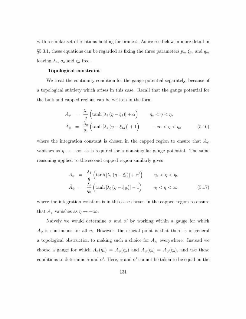
with a similar set of relations holding for brane b. As we see below in more detail in

§5.3.1, these equations can be regarded as fixing the three parameters pa, ξ2a and qa,

leaving λa, σa and ηa free.

Topological constraint

We treat the continuity condition for the gauge potential separately, because of

a topological subtlety which arises in this case. Recall that the gauge potential for

the bulk and capped regions can be written in the form

Aψ =λ1

q

(tanh [λ1 (η − ξ1)] + α

)ηa < η < ηb

Aψ =λaqa

(tanh [λa (η − ξ1a)] + 1

)−∞ < η < ηa (5.16)

where the integration constant is chosen in the capped region to ensure that Aψ

vanishes as η → −∞, as is required for a non-singular gauge potential. The same

reasoning applied to the second capped region similarly gives

Aψ =λ1

q

(tanh [λ1 (η − ξ1)] + α′

)ηa < η < ηb

Aψ =λbqb

(tanh [λb (η − ξ1b)]− 1

)ηb < η <∞ (5.17)

where the integration constant is in this case chosen in the capped region to ensure

that Aψ vanishes as η → +∞.

Naively we would determine α and α′ by working within a gauge for which

Aψ is continuous for all η. However, the crucial point is that there is in general

a topological obstruction to making such a choice for AM everywhere. Instead we

choose a gauge for which Aψ(ηa) = Aψ(ηa) and Aψ(ηb) = Aψ(ηb), and use these

conditions to determine α and α′. Here, α and α′ cannot be taken to be equal on the

131

region of overlap, ηa < η < ηb, but must differ instead by a gauge transformation.

Following standard arguments, this leads to the quantization condition

λ1

q(α− α′) =

N

e(5.18)

where N is an integer, and e is the gauge coupling for the background gauge field

(which need not equal g1 if the background flux is not the one gauging the specific

UR(1) symmetry).

We find in this way that eq. (5.18) implies the following quantization condition

on the various parameters:

N

e=

λ1

q

(tanh[λ1(ηb − ξ1)]− tanh[λ1(ηa − ξ1)]

)+λaqa

(tanh[λa(ηa − ξ1a)] + 1

)− λbqb

(tanh[λb(ηb − ξ1b)]− 1

). (5.19)

This generalizes to the case of thick branes the well-known Dirac quantization con-

dition N/e = 2λ1/q [93], which is retrieved from eq. (5.19) in the thin-brane limit

obtained by taking ηa → −∞ and ηb → +∞.

Such arguments show that in general the continuity of the gauge potential across

the two 4-branes, η = ηa and η = ηb, determines the integration constants, α and

α′ which are specific to the gauge potentials. But the topological constraint then

implies a single additional condition, eq. (5.19), which relates the bulk parameters,

λ1, ξ1 and q, to the undetermined brane quantities, ηa, ξ1a, ηb, ξ1b and the flux integer

N .

132

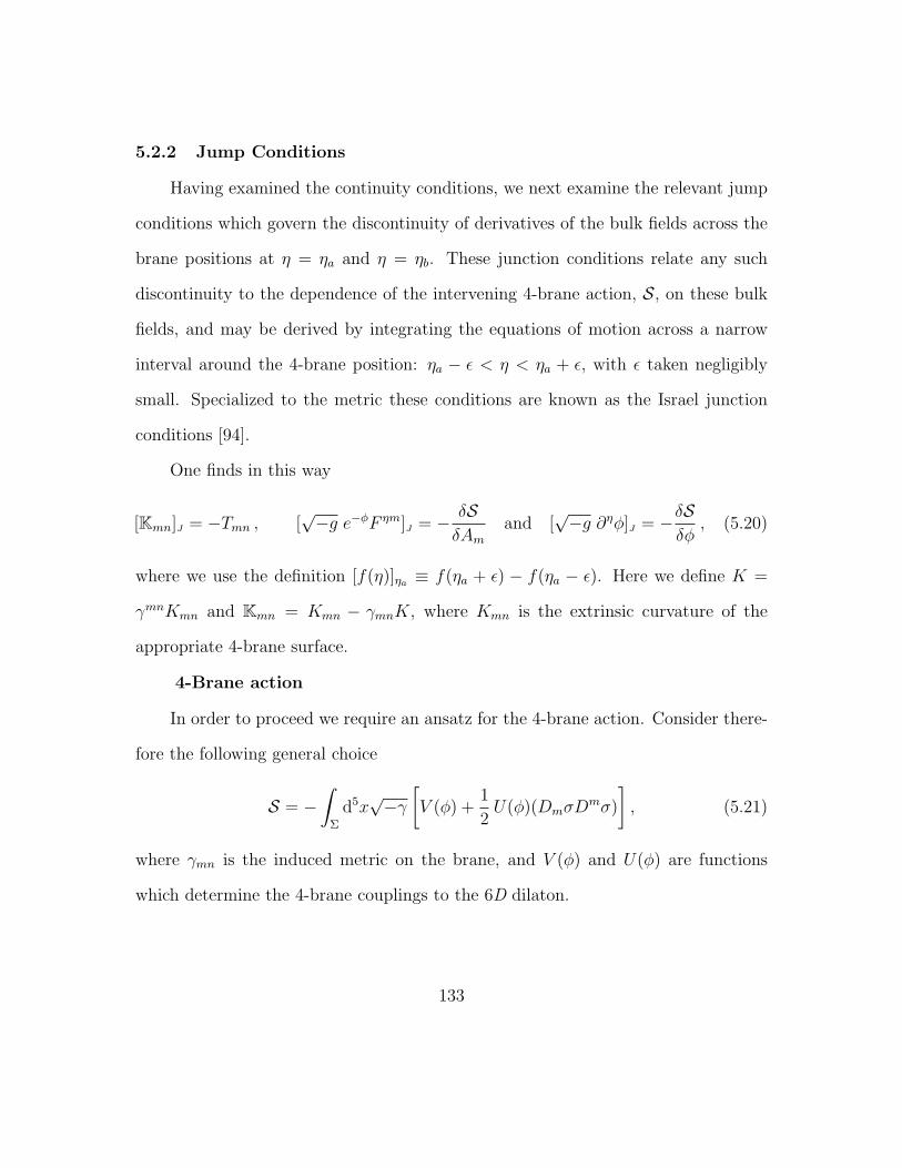
5.2.2 Jump Conditions

Having examined the continuity conditions, we next examine the relevant jump

conditions which govern the discontinuity of derivatives of the bulk fields across the

brane positions at η = ηa and η = ηb. These junction conditions relate any such

discontinuity to the dependence of the intervening 4-brane action, S, on these bulk

fields, and may be derived by integrating the equations of motion across a narrow

interval around the 4-brane position: ηa − ε < η < ηa + ε, with ε taken negligibly

small. Specialized to the metric these conditions are known as the Israel junction

conditions [94].

One finds in this way

[Kmn]J = −Tmn , [√−g e−φF ηm]J = − δS

δAmand [

√−g ∂ηφ]J = −δS

δφ, (5.20)

where we use the definition [f(η)]ηa ≡ f(ηa + ε) − f(ηa − ε). Here we define K =

γmnKmn and Kmn = Kmn − γmnK, where Kmn is the extrinsic curvature of the

appropriate 4-brane surface.

4-Brane action

In order to proceed we require an ansatz for the 4-brane action. Consider there-

fore the following general choice

S = −∫

Σ

d5x√−γ[V (φ) +

1

2U(φ)(DmσD

mσ)

], (5.21)

where γmn is the induced metric on the brane, and V (φ) and U(φ) are functions

which determine the 4-brane couplings to the 6D dilaton.

133

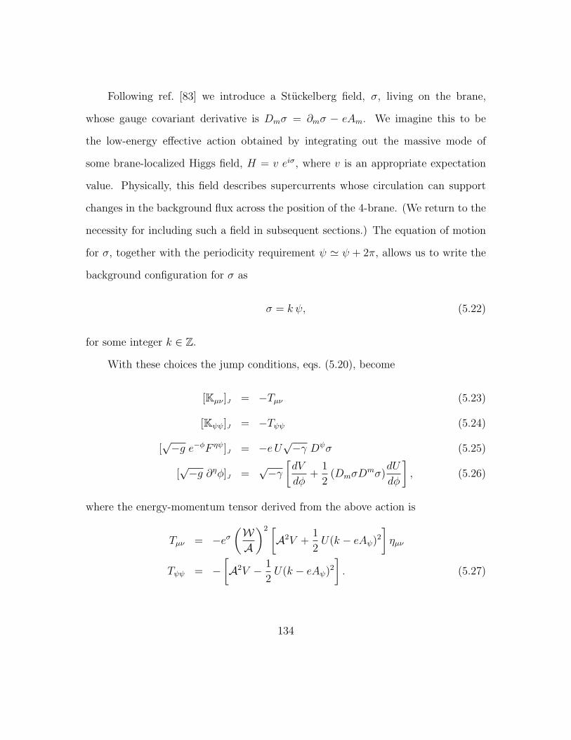
Following ref. [83] we introduce a Stuckelberg field, σ, living on the brane,

whose gauge covariant derivative is Dmσ = ∂mσ − eAm. We imagine this to be

the low-energy effective action obtained by integrating out the massive mode of

some brane-localized Higgs field, H = v eiσ, where v is an appropriate expectation

value. Physically, this field describes supercurrents whose circulation can support

changes in the background flux across the position of the 4-brane. (We return to the

necessity for including such a field in subsequent sections.) The equation of motion

for σ, together with the periodicity requirement ψ ' ψ + 2π, allows us to write the

background configuration for σ as

σ = k ψ, (5.22)

for some integer k ∈ Z.

With these choices the jump conditions, eqs. (5.20), become

[Kµν ]J = −Tµν (5.23)

[Kψψ]J = −Tψψ (5.24)

[√−g e−φF ηψ]J = −eU

√−γ Dψσ (5.25)

[√−g ∂ηφ]J =

√−γ[dV

dφ+

1

2(DmσD

mσ)dU

dφ

], (5.26)

where the energy-momentum tensor derived from the above action is

Tµν = −eσ(WA

)2 [A2V +

1

2U(k − eAψ)2

]ηµν

Tψψ = −[A2V − 1

2U(k − eAψ)2

]. (5.27)

134

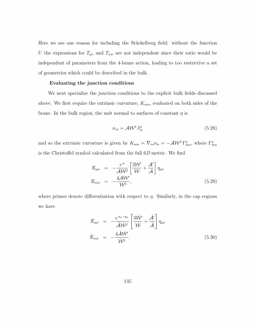
Here we see one reason for including the Stuckelberg field: without the function

U the expressions for Tµν and Tψψ are not independent since their ratio would be

independent of parameters from the 4-brane action, leading to too restrictive a set

of geometries which could be described in the bulk.

Evaluating the junction conditions

We next specialize the junction conditions to the explicit bulk fields discussed

above. We first require the extrinsic curvature, Kmn, evaluated on both sides of the

brane. In the bulk region, the unit normal to surfaces of constant η is

nM = AW4 δηM (5.28)

and so the extrinsic curvature is given by Kmn = ∇mnn = −AW4 Γηmn, where Γηmn

is the Christoffel symbol calculated from the full 6D metric. We find

Kµν = − eσ

AW2

[3W ′

W+A′

A

]ηµν

Kψψ = −4AW ′

W5, (5.29)

where primes denote differentiation with respect to η. Similarly, in the cap regions

we have

Kµν = −eσa−pa

AW2

[3W ′

W+A′

A

]ηµν

Kψψ = −4AW ′

W5. (5.30)

135

• Evaluating the (µν) Israel junction condition at η = ηa then gives5

(λ3

2+ e−2(σ−σa+λ3ηa)λa tanh[λa(ηa − ξ2a)]− λ2 tanh[λ2(ηa − ξ2)]

)= −W4

[(AVa) +

1

2

(UaA

)(ka − eAψ)2

](5.31)

where the subscript ‘a’ on V , U and k denotes the corresponding 4-brane property

specialized to the brane at η = ηa.

• The (ψψ) Israel junction condition similarly gives

[λ1 tanh[λ1(ηa − ξ1)]− λ2 tanh[λ2(ηa − ξ2)]− e−2(σ−σa+λ3ηa)

(λa tanh[λa(ηa − ξ1a)]

−λa tanh[λa(ηa − ξ2a)])]

= −W4

[(AVa)−

1

2

(UaA

)(ka − eAψ)2

]. (5.32)

Taking the sum and the difference of these last two conditions allows the isolation

of conditions for Va and Ua separately. It is also easy to see that the resulting

equations always admit real solutions for any value of the bulk parameters and the

brane position.

• The junction condition for the gauge field similarly evaluates to

q − qae−2(σ−σa+λ3ηa) = −eW4

(UaA

)(ka − eAψ). (5.33)

5 It is understood in what follows that all functions depending on η are evaluatedat η = ηa.

136

Notice that we can eliminate the two brane quantities, Ua and Va, from the pre-

vious three jump conditions to obtain a constraint that does not depend on 4-brane

parameters. Indeed, by subtracting eq. (5.31) from eq. (5.32), and then dividing the

result by eq. (5.33), we obtain the expression

12λ3 + λa tanh[λa (ηa − ξ1a)]− λ1 tanh[λ1 (ηa − ξ1)]

e−2(σ−σa+λ3ηa) qa − q

= −kae

+λaqa

(tanh[λa(ηa − ξ1a)] + 1

). (5.34)

An identical argument for brane b similarly gives:

12λ3 + λb tanh[λb (ηb − ξ1b)]− λ1 tanh[λ1 (ηb − ξ1)]

e−2(σ−σb+λ3ηb) qb − q

= −kbe

+λbqb

(tanh[λb(ηb − ξ1b)]− 1

). (5.35)

• By contrast, the dilaton junction condition gives a condition on the φ-derivatives

of Ua and Va:

2λ3 + λ1 tanh[λ1(ηa − ξ1)]− λ2 tanh[λ2(ηa − ξ2)] (5.36)

−e−2(σ−σa+λ3ηa)(λa tanh[λa(ηa − ξ1a)]− λa tanh[λa(ηa − ξ2a)]

)= −2W4

[AdVa

dφ+

1

2AdUadφ

(ka − eAψ)2],

which, using the (ψψ) Israel jump condition, simplifies to

2λ3 =W4[A(Va − 2

dVadφ

)− 1

2A

(Ua + 2

dUadφ

)(ka − eAψ)2

]. (5.37)

137

Conditions for scale invariance

Before proceeding it is useful to pause at this point to record the unique choice

for the functions Va and Ua which preserves the classical scaling symmetry of the

bulk equations of motion, corresponding to the transformation σ → σ + ∆ and

σa → σa + ∆.

Inspection shows that the continuity equations remain unchanged by this trans-

formation because σ and σa only appear there in the combination σ − σa. The

left-hand-sides of the various jump conditions remain similarly unchanged. On the

right-hand-side, however, we see that A transforms, and so invariance requires Va(φ)

and Ua(φ) to transform in a way which cancels the transformation of A. Such an

invariant choice for Ua and Va is possible for the Israel and Maxwell jump conditions,

eqs. (5.31), (5.32), and (5.33), because within these Ua and Va only appear with A in

the combinations AVa and Ua/A. It follows that preservation of the classical scaling

symmetry requires

Va = vaeφ/2 and Ua = uae

−φ/2 , (5.38)

in agreement with the analysis of ref. [51]. Any other choices for these functions

necessarily breaks the classical scale invariance of the problem.

It then remains to determine what invariance requires for the dilaton jump con-

dition, eq. (5.37). When this is specialized to the scale invariant case, eqs. (5.38),

the right-hand side degenerates to zero, giving the simple condition λ3 = 0. Besides

imposing no new conditions on Ua and Va, this tells us that scale-invariant brane con-

figurations can only source bulk geometries satisfying λ3 = 0, and hence only having

138

conical singularities. Since all of the geometries having two conical singularities are

4D-flat [1], we see in detail how the jump conditions enforce the connection between

scale invariance and 4D flatness.

5.3 Applications

Given the general bulk and cap solutions, and a complete set of matching condi-

tions, we may now see what the solutions to these conditions tell us about bulk-brane

dynamics in six dimensions. In this section we use the above formalism to address

two questions. First: given a bulk geometry what kinds of caps are possible? Second:

given specific brane properties, what kinds of bulk are generated? In particular, in

this second case we ask how the breaking of scale invariance by the branes can lead

to the stabilization of the extra-dimensional size.

Answering this last question allows us also to address an issue of potential im-

portance for phenomenology: what conditions must the cap and bulk parameters

satisfy in order to have a large hierarchy between the volumes of the caps and the

volume of the bulk? This point is important when the regularizing 4-branes and

caps are regarded as specifying the microscopic structure of 3-branes that sit at the

singular points of the geometry.

5.3.1 Capping a Given Bulk

We begin by studying what kinds of caps can be used to smooth a generic bulk

solution. In this section we therefore regard the 5 bulk parameters λ1, λ2, ξ1, q

and σ as given (we remove both p and ξ2 using appropriate coordinate conditions),

and look for solutions for the kinds of branes which can smooth the singularities at

η = ±∞.

139

We emphasize that our purpose here is simply to show that a regularization

procedure exists for any choice of bulk solution, through an appropriate choice for

the 4-branes and caps. We return in subsequent sections to the relations which must

exist between the parameters governing the branes and caps, due to the interpolation

between them of a 4D-flat bulk.

Parameter counting

It is instructive to count parameters and constraints, to get a sense of whether

or not the problem of capping a given bulk is over-determined. To this end it is

worth distinguishing between those parameters which are integration constants in the

capped region, and those which arise within the action, S, governing the 4-brane. We

start by counting only those relations which are independent of the 4-brane action,

before returning to those which are not.

S-independent conditions: We have seen that each cap naively involves 7 integration

constants, λa, ξ1a, ξ2a, pa, qa, σa and ηa that are related by the smooth-geometry

condition, (5.9), at each cap. Counting the two caps this gives a total of 6 + 6 = 12

independent cap integration constants.

At each cap these parameters are subject to 3 continuity conditions, eqs. (5.13)

– (5.15), as well as the 1 jump condition, (5.34) or (5.35), constructed by eliminating

U(φ) and V (φ) from eqs. (5.31) – (5.33). The topological constraint then imposes

one more overall relation which relates the properties of the bulk to those of both

caps, giving a grand total of 4 + 4 + 1 = 9 conditions. Barring other obstructions we

then expect to find a 12 − 9 = 3-parameter family of capped geometries which can

match properly to the given bulk.

140

S-dependent conditions: In addition to these are the parameters Ua(φ) and Va(φ)

governing the 4-brane action, S. For each brane these two functions are related by

the three remaining conditions, eqs. (5.31), (5.32) and (5.37). Solving the two linear

equations, (5.31) and (5.32), immediately gives Ua and Va as explicit functions of ηa:

Ua = Ua(ηa) and Va = Va(ηa) (where we suppress the dependence on the other cap

and bulk parameters).

We are then left with one remaining relation: the dilaton jump condition,

eq. (5.37). Since this requires knowing the derivatives, dUa/dφ and dVa/dφ, further

progress requires making some choices for the functional form of these quantities.

• If Ua and Va are both constant, then both are fixed by eqs. (5.31) and (5.32).

In this case the dilaton jump condition, eq. (5.37), imposes an additional 2

constraints (one at each cap) on the 3 cap integration constants which remain

to this point undetermined. We are then led to expect a 1-parameter family of

capped solutions.

• If Ua and Va preserve scale invariance, then Ua = ua e−φ/2 and Va = va e

φ/2,

have 2 free parameters. In this case the counting naively goes through as above,

with one change: although ua and va are fixed by solving the Israel junction

conditions, eqs. (5.31) and (5.32), the dilaton jump condition, eq. (5.37), degen-

erates to λ3 = 0 and so does not further constrain any 4-brane or cap param-

eters. (None of these matching conditions fix the scale symmetry σ → σ + ∆,

σa → σa + ∆ and σb → σb + ∆. However, because we here regard the bulk

141

parameter σ to have been specified this symmetry does not preclude the de-

termination of σa and σb in terms of σ.) We are therefore led in this case to 3

free parameters in the capped solution.

• More general choices for Ua and Va potentially involve more parameters, and

so allow more freedom of choice for the capped geometry. For instance, if

Ua = ua esaφ and Va = va e

taφ, then the three conditions, (5.31), (5.32) and

(5.36), provide three relations amongst the four parameters ua, va, sa and ta,

and in particular (5.36) no longer constrains the parameters of the caps. In this

case we’d expect a total of 5 free parameters to describe the capped geometry.

Considerations such as these lead us to expect that capped solutions of the

type we entertain should exist for any given kind of bulk geometry, barring an ob-

struction to solving the relevant equations. Furthermore, we expect to find at least a

1-parameter family of such solutions, and this has a simple physical interpretation: in

the absence of the topological constraint the caps have 2 free parameters, correspond-

ing to the freedom to choose the positions, ηa and ηb, where we choose to position the

two caps. The topological constraint can then impose one relation amongst these

two positions, relating them to the quantum number, N , which governs the total

amount of Maxwell flux.

Notice that our counting here regards U and V as parameters to be adjusted

even though these arise within the brane action rather than as integration constants

in the solutions to the field equations. So the existence of the caps requires these

parameters in the action to be tuned relative to one in a way which depends on the

properties of the given bulk solution. We also do not distinguish here whether the

142

solutions found give positive values for U and V , as would normally be required by

positivity of the kinetic energy associated with brane motion (V ) and the Stuckelberg

field (U).

Freely-floating 4-branes

The previous section takes the point of view that the φ-dependence of the 4-

brane action can be arbitrarily parameterized, with the parameters required to cap

the given bulk geometry being fixed in terms of the positions of the caps and other

variables. Another point of view is to ask for a 4-brane action to be defined so

that the same 4-brane action can be used at any 4-brane position, for a given bulk

geometry. As we shall see, consistency also requires the cap geometry to be varied

as a function of the brane position. This approach is similar in spirit to what is done

for the actions of end-of-the-world branes which mark the boundary of bulk spaces

in discussions of the AdS/CFT correspondence [95].

This amounts to asking that the ηa-dependence inferred by solving eqs. (5.31)

and (5.32) for Ua(ηa) and Va(ηa) is completely given by the implicit ηa-dependence

which Ua and Va inherit as functions of φ(ηa) (with ηa-independent constants). That

is, we demand Ua(ηa) = Ua[φ(ηa)] and Va(ηa) = Va[φ(ηa)]. We call such a 4-brane

action the ‘floating’ action which is defined by the given bulk and capped geometries.

In principle, the functional form that this requires for both Ua(φ) and Va(φ) can be

inferred in this way using the known expressions for the bulk dilaton profile, φ(ηa),

together with the expressions for Ua(ηa) and Va(ηa) obtained by solving eqs. (5.31)

and (5.32).

143

Finally, the dilaton jump condition, (5.37), is then read as an additional con-

straint on the parameters which govern the capped geometry. To identify this con-

straint more explicitly, we notice that we could use either the bulk dilaton profile,

φ(η), or the profile in the cap, φ(η), to convert the ηa dependence of Ua and Va

into their dependence on the dilaton. In particular, we have two ways of evaluating

the dilaton derivative of the 4-brane quantities like Ua, which must agree with each

other: (dUadηa

)=

(dUadφ

)φ=φ(η)

(dφ

dηa

)=

(dUadφ

)φ=φ(η)

(dφ

dηa

). (5.39)

Here dφ/dηa = (∂φ/∂η)|η→ηa , while dφ/dηa also includes the implicit dependence on

ηa that that φ acquires through its dependence on the ηa-dependent cap parameters.

Collectively denoting these cap parameters by cs = λa, ξ1a, . . . , we have

dφ

dη=

[(∂φ

∂η

)+

(∂φ

∂ cs

)∂ cs∂ηa

]η→ηa

. (5.40)

The desired consistency condition on the cap parameters comes from equating

(∂φ/∂η)η→ηa obtained by solving eqs. (5.39) and (5.40), with that inferred from the

dilaton jump condition, eq. (5.37).

We see from this that the number of independent constraints on the cap ge-

ometry is the same as it was when we made the simpler assumption that U and V

were constants. We have not yet tried to solve these constraints to determine the

functional form for Ua(φ) and Va(φ) which would be obtained.

Solving the matching conditions

In order to see in more detail if obstructions to solutions to the matching con-

ditions might exist, we next examine some of these conditions in more detail. Recall

144

that if if the smoothness condition is not used then each cap is described by 7 in-

tegration constants — λa, qa, ξ1a, ξ2a, σa, pa and ηa — for a total of 14 once both

branes are included. Smoothness of the caps and continuity at both branes, with

the topological condition cut these down by a total of 9 conditions, leaving 5 un-

determined. There is also one combination of jump conditions at each brane which

does not involve the potentials U and V , reducing us to 3 parameters. If U and V

are φ-independent, then the dilaton jump condition for each brane removes 2 more.

This leaves 1 cap parameter undetermined. By contrast, the integers ka, kb and N

describing the monopole flux and background configuration for the Stuckelberg field

are not solved for, but are instead regarded as choices we get to pick by hand. We

show there is a solution to the junction conditions for a range of ka, kb and N .

In what follows it is convenient to define first the quantities

Λia = λa(ηa − ξia), Λib = λb(ηb − ξib), (5.41)

and ∆ia = λi(ηa − ξi), ∆ib = λi(ηb − ξi) (5.42)

where i = 1, 2. In our counting, the parameters Λia and Λib replace ξia and ξib,

whereas ∆ia and ∆ib are known functions of ηa and ηb.

Recall that there are a total of 14 cap parameters, and these are subject to a

total of 11 conditions before the three conditions (per brane) involving U and V are

used, leaving 3 parameters undetermined. (Depending on what we assume about

the 4-brane action — such as if U and V are constants — two of these can then

be fixed by the dilaton jump conditions, leaving the single undetermined parameter,

although we do not yet apply this constraint in this section.) Although other choices

145

are possible, we find it easiest to solve for the cap parameters as functions of the

three undetermined quantities (ηa, ηb,Λ1b).

We start with the topological constraint, eq. (5.19), which we simplify by using

eq. (5.13) and its counterpart for brane b to eliminate the combinations λa/qa and

λb/qb. Using the resulting expressions in eq. (5.19) gives

tanh ∆1b − tanh ∆1a =qN

eλ1

− εa eΛ1a

cosh ∆1a

− εb e−Λ1b

cosh ∆1b

, (5.43)

where we define εa = |qa|/qa = sign qa, and similarly for εb and ε. Writing this as

εaeΛ1a = F , with F = F (ηa, ηb,Λ1b) given by

F = cosh ∆1a

(qN

eλ1

− εbe−Λ1b

cosh ∆1b

− tanh ∆1b + tanh ∆1a

), (5.44)

shows that solutions exist so long as we choose εa = signF , and gives these solutions

as

Λ1a = ln |F | . (5.45)

Using the smoothness condition together with the continuity condition, eq. (5.13),

and the above solution for Λ1a, then gives

Λ2a = ln

∣∣∣∣λ1ga(1 + F 2)

q cosh ∆1a

∣∣∣∣ . (5.46)

As we have now solved for Λ1a and Λ2a in terms of ηa, ηb, and Λ1b, we do not bother

to eliminate these two parameters from future expressions.

146

We next solve for λa. Starting from eq. (5.34) and using the continuity conditions

to simplify further, we arrive at the expression

λa =1

tanh Λ1a

(λ1 tanh ∆1a −

λ3

2(5.47)

+

[1− εεagaλ2 cosh ∆1a cosh Λ2a

g1λ1 cosh ∆2a cosh Λ1a

] [qkae− εaλ1e

Λ1a

cosh ∆1a

]).

It is important to note that by choosing the integer ka appropriately, we can ensure

λa > 0.6 Again, as we have solved for λa in terms of the three required parameters,

we will not need to eliminate it from future equations. Finally, the 3 continuity

equations at brane a directly give

pa = λ3ηa, (5.48)

qa =

(εqλaλ1

)(2F

1 + F 2

)cosh ∆1a, (5.49)

σa = σ + λ3ηa +1

2ln

∣∣∣∣ gaλ2 cosh Λ2a

g1λa cosh ∆2a

∣∣∣∣ . (5.50)

The analysis at brane b is similar, for which we find

Λ2b = Λ1b + ln

∣∣∣∣ q cosh ∆1b

2λ1gb cosh Λ1b

∣∣∣∣ , (5.51)

λb =1

tanh Λ1b

(λ1 tanh ∆1b −

λ3

2(5.52)

+

[1− εεbgbλ2 cosh ∆1b cosh Λ2b

g1λ1 cosh ∆2b cosh Λ1b

] [qkbe

+εbλ1e

−Λ1b

cosh ∆1b

]),

6 One might worry that this is no longer true if the first term in square bracketsis zero, but a little work shows that the condition for this term being nonzero (forarbitrary ka) is equivalent to the condition Ua 6= 0, which we assume.

147

and

pb = λ3ηb, (5.53)

|qb| =

(|q|λbλ1

)cosh ∆1b

cosh Λ1b

, (5.54)

σb = σ + λ3ηb +1

2ln

∣∣∣∣ gbλ2 cosh Λ2b

g1λb cosh ∆2b

∣∣∣∣ . (5.55)

By using the previous expressions for Λ2b and λb, we see that we have solved for |qb|

and σb in terms of the required 3 parameters. The sign of qb can be determined by

the gauge field jump condition at brane b.

This exhausts all of the matching conditions which do not involve the 4-brane

coupling functions. The value of these functions, U and V , at each brane is then easily

obtained by solving the Israel junction conditions, eqs. (5.31) and (5.32), leaving only

the dilaton jump condition to be solved. If U and V contain enough parameters to

allow them and their derivatives to be varied independently for each brane, then this

last condition can be solved without adding further constraints on the parameters of

the cap geometry.

5.3.2 Bulk Geometries Sourced by Given Branes

In the previous section the bulk geometry is considered to be given, and we ask

whether regularizing caps can be constructed. This section adopts a different point

of view, wherein the characteristics of the caps — i.e. all the integration constants

that define the cap geometry and the quantities U and V — are given, and we seek

the properties of the bulk which results. In particular, our interest is to see whether

and how the two caps must be related to one another, and to check whether the bulk

148

configuration is always of the form of a GGP solution, with flat four-dimensional

slices.

Our goal in doing so is two-fold. First, in this section, we wish to see whether

this reduced problem is over-determined, and if so what is required in detail of the

branes in order to ensure a solution. Secondly, in §5.3.3 we set out to understand

how the volume of the bulk geometry is related to the brane properties, and, by

doing so, to exhibit a stabilization mechanism for the bulk volume. Of particular

interest is then to understand what 4-brane/cap properties are required to ensure

the volumes of the capped regions are much smaller than that of the intervening bulk

(as is required if the 4-branes and caps describe the microscopic structure of more

macroscopic 3-branes).

Parameter counting and junction conditions

We now show that counting equations and parameters suggests we are not com-

pletely free to specify the 4-brane action for brane a arbitrarily if we ask that it

interpolate between 4D-flat cap and bulk geometries. This can be done only if the

4-brane action is subject to one constraint equation (as was argued in ref. [71]),

but once this is satisfied there is sufficient information to determine the parameters

describing both the bulk geometry and the properties of brane b.7

7 To be precise, we find a two parameter family of solutions for the bulk and capb, corresponding to where we choose to embed the two branes in the bulk. Once thischoice is made, then the bulk and cap b are unique.

149

To this end, imagine we specify the cap geometry and 4-brane action at a given

position η = ηa. Next recall that there are 7 integration constants characterizing the

the bulk geometry — λ1, λ2, ξ1, ξ2, p, q and σ. (Notice that, although previously we

have removed two of these quantities — ξ1 and p — by suitably adjusting coordinates,

this is typically no longer possible without altering the specified parameters for cap

a.) These 7 parameters are subject to a total of 7 conditions at ηa, consisting of 3

continuity conditions (metric and dilaton) and 4 jump conditions (Israel, Maxwell

and dilaton), suggesting that the bulk parameters are completely specified in terms

of those of the cap and 4-brane at ηa.

As we show in the next section, however, one of these seven equations which is

supposed to determine one of the bulk parameters turns into a constraint equation

amongst cap and brane parameters. Thus, what we find is that for any given cap

and brane which satisfies the constraint, there is a one-parameter family of flat bulks

to which we can match. Physically, it is easiest to interpret this one parameter in

the coordinate system where ξ1 = ξ1a = 0. Recall that in this coordinate system

the brane location in the bulk and cap is ηa and ηa, respectively, where these two

numbers are generically not the same. Here, we again imagine fixing the cap and

brane properties at ηa, and then solving for six of the seven bulk parameters: λ1, λ2,

ξ2, σ, p, q, and ηa. Thus, this one-parameter family of bulk solutions corresponds

to where we choose to place the brane in the bulk coordinate system. If ηa is fixed,

then we find a unique solution for the bulk.

Continuing to use the coordinate system where ξ1 = ξ1a = ξ1b = 0, we see that

once the bulk geometry is thus inferred, there remain 10 parameters associated with

150

cap b, consisting of 6 integration constants — λb, qb, ξ2b, σb, pb, and ηb — plus the

brane position ηb in the bulk coordinate system, the two 4-brane parameters, Ub and

Vb, and one linear combination of their derivatives. These 10 parameters are then

subject to 9 conditions, consisting of the 7 continuity and jump conditions at the

brane location, the smoothness condition at η → ∞ for cap b and the topological

constraint on the Maxwell field. Provided there are no obstructions to solving these

equations, this shows that once we choose the properties of one brane (subject only to

the Hamiltonian constraint), together with the location of the two branes in the bulk

coordinate system, ηa and ηb, then properties of the other brane and the intervening

4D-flat bulk are precisely dictated. If the properties of brane b are not adjusted

in this way in terms of those of brane a then the intervening bulk solution cannot

be 4D flat, and instead must either be 4D maximally symmetric but not flat [1] or

time-dependent and not Lorentz invariant [2].

This counting bears out, and make more precise, expectations based on earlier

studies of the general properties of bulk solutions to 6D supergravity. In partic-

ular, for 4D maximally-symmetric solutions [1] (including those which are not 4D

flat) the bulk geometry depends nontrivially only on η, and so we may imagine in-

tegrating the bulk field equations in the η direction, starting at brane a and ending

at brane b. Since the η-η Einstein equation does not involve second derivatives of

the metric, it represents a ‘Hamiltonian’ constraint on those ‘initial’ conditions at

brane a which can be consistently used for such an integration. In this language,

the above-mentioned constraint on the allowed 4-brane parameters corresponds to

requirements imposed on the 4-brane by matching to the Hamiltonian constraint in

151

the bulk, restricted to 4D-flat geometries [71]. Furthermore, since the bulk geome-

try is completely specified by integrating forward in η using the ‘initial’ conditions

at brane a, its asymptotic form at brane b is seen to be completely determined, in

agreement with what we find here for explicit 4-brane/cap regularizations of this

asymptotic form.

Explicit solutions

To better see if parameter and equation counting provides the whole story, we

next solve the matching to see whether obstructions to their solutions can exist.

The Bulk

The continuity equations, eqs. (5.13) – (5.15), read in this case:

|q| = |qa|(λ1 cosh Λ1a

λa cosh ∆1a

), (5.56)

e−2σ = e−2(σa−λ3ηa)

(gaλ2 cosh Λ2a

g1λa cosh ∆2a

), (5.57)

p = pa − λ3ηa , (5.58)

and can be thought as fixing the bulk parameters q, σ, and p (recall the definitions

of the parameters Λ and ∆ in formulae (5.41) and (5.42)). Note that the sign of q is

not yet fixed. These solutions are given in terms of the four bulk quantities λ1, λ2,

∆1a, and ∆2a, for which we now solve.

152

Before proceeding it is convenient to first define four combinations of brane and

cap parameters:

C1 =

(ga cosh Λ2a

2g1λa

)[AW4(Va − 2V ′a)−

W4

2A(Ua + 2U ′a)(ka − eAψ)2

], (5.59)

C2 =

(ga cosh Λ2a

4g1λa

)[AW4(5Va − 2V ′a)

+W4

2A(3Ua − 2U ′a)(ka − eAψ)2 + 4λa tanh Λ2a

], (5.60)

C3 =

(εaga cosh Λ2a

g1 cosh Λ1a

)[−eUaqa

(W4

A

)(ka − eAψ) + 1

], (5.61)

C4 =

(ga cosh Λ2a

4g1λa

)[AW4(Va − 2V ′a)

+W4

2A(7Ua − 2U ′a)(ka − eAψ)2 + 4λa tanh Λ1a

], (5.62)

where primes here denote differentiation with respect to φ. These four parameters

will take the place of Ua(ηa), Va(ηa), their derivatives (which appear in only one

linear combination), and ka. The action for brane a can therefore be equally well

characterized by these four quantities, as by our original parameterization in terms

of Ua(ηa), Va(ηa), and derivatives. With these definitions in hand, the remaining four

matching conditions reduce to the following equations:

C1 = cosh ∆2a

[1−

(λ1

λ2

)] 12

(5.63)

C2 = sinh ∆2a (5.64)

C3 = ε

(λ1

λ2

)cosh ∆2a

cosh ∆1a

(5.65)

C4 =

(λ1

λ2

)tanh ∆1a cosh ∆2a. (5.66)

153

Recalling that both λ1 and λ2 are positive, we see immediately that ε ≡ sign q =

sign C3.

We note that this system of equations is over-determined, since there are four

equations but only three unknowns: ∆1a, ∆2a, and λ1/λ2. In fact, by squaring the

above equations it is straightforward to check this constraint is given by

C21 − C2

2 + C23 + C2

4 = 1. (5.67)

When the above equation is satisfied, then it can be shown that the bulk fields satisfy

the Hamiltonian constraint which ensures 4D flatness.8 Henceforth, we assume that

the brane properties are chosen such that the Hamiltonian constraint is satisfied. In

this case, the solution to eqs. (5.63) - (5.66) is

∆1a = sign(C4) arcosh

[(1 +C2

4

C23

) 12

], (5.68)

∆2a = arsinh(C2), (5.69)

λ1

λ2

=

(1− C2

1

C21 + C2

3 + C24

) 12

. (5.70)

where the range of arcosh is taken be x ∈ R : x ≥ 0. It is easy to see that solutions

to these equations exist for any values of the Ci, subject only to the constraint that

they obey eq. (5.67).

As expected from the arguments in the previous section, we indeed find a one-

parameter family of possible bulks. Once this parameter is fixed — corresponding

8 This Hamiltonian constraint is given by eq. (34) in reference [1].

154

to choosing where in the bulk we wish to embed the brane — then the bulk solution

becomes unique. Henceforth, we assume that this choice has been made (as can be

accomplished by making a specific choice for p in eq. (5.58)).

Cap b

Having uniquely determined the bulk solution, it remains to determine the properties

of the 4-brane and cap at brane b. In order to find a unique solution, we first specify

the location where we wish to cap the bulk, ηb. Since this analysis is identical to that

of §5.3.1, we do not repeat it in detail here, however the three continuity conditions,

the smoothness condition, and the combination of the jump conditions which is

independent of Ub and Vb provide 5 constraints on the 5 cap integration constants pb,

Λ2b, λb, qb and σb (see eqs. (5.51) - (5.55)). Then, the two Israel junction conditions

fix Ub and Vb, and the dilaton jump condition provides the constraint which fixes the

one relevant combination of derivatives U ′b and V ′b . The only cap parameter which is

not fixed by these conditions is Λ1b, and this can be determined from the topological

equation (5.43). As expected [1], both the properties of the bulk and those of the

4-brane and cap at η = ηb are dictated by those of the brane and cap at η = ηa.

5.3.3 Volume Stabilization and Large Hierarchy

The previous analysis fixing the seven bulk integration constants in terms of

given cap parameters fixes in particular the integration constant, σ, that parame-

terizes the bulk volume. This provides a natural 6D mechanism for stabilizing this

bulk volume. In this section we explore this stabilization in more detail, focussing on

the conditions which are required to obtain a large hierarchy between the volumes

155

of the bulk and the caps. In the next section we identify the low-energy 4D effective

potential which is generated in this way for σ.

Conditions for a hierarchy

We now ask for the conditions the brane and cap actions should satisfy to ensure

that the cap volumes are much smaller than those of the bulk. Our point of view

here is that the bulk geometry is given, and so would like to phrase the conditions

for a hierarchy in terms of only those parameters over which we have control: the

bulk parameters and the three cap parameters, ηa, ηb, and Λ1b.

In order to have branes whose circumference is small, we seek to ensure A(ηa)

and A(ηb) are much less than one. We see from eq. (5.4) that it is natural to examine

for this purpose the limit ηa → −∞ and ηb →∞, although in general this need not be

sufficient in itself to have small cap volumes. However, we now argue that sufficient

conditions for obtaining small cap volumes are given by

Λ1a = λa(ηa − ξ1a) −1

Λ2a = λa(ηa − ξ2a) −1 (5.71)

with similar conditions for brane b. Large, negative ηa is not sufficient for small cap

volumes because it does not in itself ensure that these conditions are satisfied. Under

these conditions we may use the asymptotic form for the hyperbolic functions and

so obtain the following expression for volume of cap a

Ωa = 2π

∫ ηa

−∞dη A2W4

' π

λae2(σ−σa+pa)(A2W4)|ηa (5.72)

156

In arriving at the second line we have used the continuity equations, (5.11), to relate

cap functions to bulk functions. The cap volume must be compared with the bulk

volume, given by the expression

Ωbulk = 2π

∫ ηb

ηa

dη A2W 4

=

((2π)2 λ1λ

32 e

2σ

(2g1)3 q

) 12 ∫ ηb

ηa

dηeλ3η

cosh32 [λ2 (η − ξ2)] cosh

12 [λ1 (η − ξ1)]

.(5.73)

It is simple to check that the integral in the previous expression is always finite.

Then, it is enough to choose the parameters in the bulk of order one, to obtain

Ωbulk ' O(1). In order to obtain a hierarchy between bulk and cap volumes, it is

necessary to demand that Ωa O(1).

We now evaluate the cap volume using the general solutions found earlier. If we

also use the hierarchy assumptions, eq. (5.71), and the continuity equation (5.14),

we calculate the cap volume to be

Ωa ' 2π

(g1 λ1 cosh ∆2a

|q|λ2 cosh ∆1a

)(A2W4)|ηa

= πA2|ηa . (5.74)

For the generic situation of O(1) bulk parameters, we see from eq. (5.4) that A2|ηa

1 in the limit of large |ηa|. Thus, we obtain the desired result: Ωa Ωbulk ∼ O(1).

Alternatively, if we instead wish to have cap volumes which are O(1) and bulk

volumes which are much larger, we simply need to choose σ 1 while keeping all

other bulk parameters fixed.

157

It remains now to show what conditions must be imposed on the bulk parameters

and cap parameters in order to ensure that conditions (5.71) are satisfied. To simplify

this discussion, we only consider the case λ3 = 0. We accomplish this by adjusting

the background gauge coupling, e, so that it is approximately equal to its value,

e0 = qN/(2λ1), in the absence of caps. More precisely, if we define

ε =1

2e−λ1(ηa−ξ1)

[qN

λ1e− 2

], (5.75)

then we should take

ε 1 and Λ1b 1 (5.76)

and, for definiteness, take ηa ≈ −ηb. In this case, the general cap solutions found

earlier satisfy the desired hierarchy conditions (5.71). The analogous hierarchy con-

ditions at brane b are much simpler to satisfy since we get to choose freely Λ1b. For

example, choosing ηb large and Λ1b ∼ ∆1b 1 guarantees that Λ2b 1 and so the

two hierarchy constraints are satisfied.

To summarize, we see here how to obtain regularizing caps which are much

smaller than the bulk volume, by appropriately tuning the gauge coupling e and by

choosing large coordinate values for the brane positions. We have also shown that

requiring such a hierarchy at only a single brane is not difficult to achieve in the

sense that it involves no tuning of any bulk parameters.

5.3.4 Low-energy 4D Effective Potential

We next dimensionally reduce the capped bulk to 4 dimensions in order to

identify more explicitly how the 4-brane action influences the stabilization of the

158

would-be flat direction parameterized by σ. In this section we restrict ourselves to

evaluating the effective 4D potential for σ within the classical approximation.

To this end we identify the effective 4D action Seff =∫

d4x Leff by computing

the 6D action at a one-parameter family of classical solutions labelled by the constant

σ:

Seff = Sa + Sb + Scap a + Sbulk + Scap b , (5.77)

where Sa =∫

d5x La and Sb =∫

d5x Lb represent the 4-brane action for caps a and b,

given by eq. (5.21), while SM =∫M

d6xL+SGH(∂M) represents the 6D bulk action,

including the Gibbons-Hawking boundary contribution, defined by eq. (5.7). The

three last terms correspond to dividing the integration over the 2 extra dimensions

into the three intervals defining the bulk, cap a or cap b.

Following [51], we see that using the 6D field equations, (2.4), to simplify the

6D bulk action in a region M with boundaries leads to the simple expression (with

κ2 = 1)

Scl =1

2

∫M

d6x√−gφcl −

∫∂M

d5x√−γ Kcl , (5.78)

which, together with Gauss’ Law, allows the last three terms in eq. (5.77) to be

written

Scap a+Sbulk+Scap b = −1

2

∫d5x

([√−g ∂ηφ+2

√−γ K]ηa+[

√−g ∂ηφ+2

√−γ K]ηb

),

(5.79)

where as before [f(η)]ηa = f(ηa + ε)− f(ηa − ε) (and similarly for ηb).

Writing Seff =∫

d4xLeff , and evaluating the right-hand-side of this last expres-

sion using the Israel and dilaton jump conditions, (5.31), (5.32) and (5.36) finally

159

gives

Leff = 2π∑i= a,b

AW4e2(σ−p)[(−Vi +

5Vi4− 1

2

dVidφ

)(5.80)

+1

2A2

(−Ui +

3Ui4− 1

2

dUidφ

)(ki − eAψ)2

]= π

∑i= a,b

AW4e2(σ−p)[(

Vi2− dVi

dφ

)− 1

2A2

(Ui2

+dUidφ

)(ki − eAψ)2

].

Finally, to make the σ-dependence explicit we write A = A0eσ/2, φ = φ0 − σ, and

choose for concreteness V (φ) = v es φ and U(φ) = u et φ. Identifying Veff = −Leff , we

find

Veff(σ) =∑i= a,b

[CV i e

(5/2−si)σ + CUi e(3/2−ti)σ

], (5.81)

where

CV i = π

[A0W4

(1

2− si

)vi e

siφ0−2p

]η=ηi

CUi = −π2

[W4

A0

(1

2+ ti

)ui e

tiφ0−2p(ki − eAψ)2

]η=ηi

. (5.82)

It is clear that this potential generically only has runaway solutions when both

CUi and CV i and both of the coefficients of σ in the exponents have the same sign,

but has nontrivial minima when some of these signs differ. Given the explicit relative

sign appearing in eqs. (5.82), and positive ui and vi, we expect that stabilization of

σ to be fairly generic.

160

The scale invariant case

Of particular interest is the case of scale-invariant branes, for which we have

si = 1/2 and ti = −1/2. In this case, not only do we recover the generic scale-

invariant form for the potential

Veff(σ) = C e2σ with C =∑i= a,b

(CUi + CV i

), (5.83)

but we also learn that C = CUi = CV i = 0. This agrees, and makes more precise, the

arguments of ref. [51], wherein the same conclusion was drawn when scale-invariant

branes were characterized as delta-function sources.

5.4 Discussion

In this chapter we present a regularization procedure for resolving the singular-

ities in the most general axially symmetric, 4D-flat solutions to 6D gauged, chiral

supergravity. This procedure resolves the singularities of these geometries using an

explicit, but broad, class of cylindrical 4-branes that couple with the bulk Maxwell,

dilaton and gravitational fields. The space interior to these 4-branes is capped off

using the most general smooth, 4D-flat, and axially symmetric solutions to the same

6D supergravity equations that were used in the bulk between the two branes. Our

analysis provides the necessary tools required to precisely explore the connections

between properties of the bulk field configurations and the structure of the branes

which source them.

We keep our analysis very general, with the goal of being able to map out these

connections with as few restrictions as possible. We show, in particular, that the class

of caps and 4-brane actions we consider contain sufficient numbers of parameters

161

to cap an arbitrary axially-symmetric and 4D-flat bulk geometry. We also show

that once the properties of one of the 4-brane caps is specified, there are sufficient

parameters in the bulk geometry and in the other cap to complete the geometry.

This both identifies the properties of the bulk sourced by a given brane, and precisely

identifies how the properties of the brane at the other end of the bulk are dictated

by those of the source brane with which one starts.

Knowing the properties of the caps shows that the presence of regularizing branes

has important consequences on the properties of the bulk solutions. In particular, we

show how the classical degeneracy amongst bulk geometries having different volumes

can be lifted by the coupling of the 4-branes with the 6D dilaton. This provides

a stabilization mechanism for the bulk, which relates the size of the extra dimen-

sions with brane properties. By performing a dimensional reduction we also identify

the effective 4D potential which captures this stabilization mechanism in the low-

energy limit. We are able to do because our regulated 6D configurations are smooth

everywhere, with the bulk fields not diverging at the brane positions (as they do

for the effective codimension-2 3-branes obtained in the thin-brane limit when the

circumference of the 4-brane is taken to zero).

162

CHAPTER 6Ultraviolet Sensitivity in Higher Dimensions

In this chapter, we calculate the size of the one-loop quantum corrections induced

by bulk loops for various supergravities in higher dimensions. As explained in the

introductory chapter, the success of the SLED proposal relies on these one-loop

effects being of order 1/r4c ∼ m4

sb in the effective 4D potential, where we recall rc is

the compactification radius and msb ∼ M2EW/MPl ∼ 10−3 eV is the supersymmetry-

breaking scale in the bulk. At this point, it is important to emphasize again that

within the SLED proposal, the Casimir energy on the brane itself is not required to

be small. This is a direct consequence of the fact that such an energy does not give

rise to a 6D cosmological constant, but instead a localized energy density∫

d4x√g ρ

which is indistinguishable from a brane tension.

Thus, when we integrate out the SM brane fields to obtain the low-energy cos-

mological constant, this has the effect of simply renormalizing various brane tensions.

The marvel of the SLED proposal occurs when we proceed to integrate out the bulk

fields in the presence of the above pure tension branes. At the classical level this

amounts to substituting their equations of motion into the action, yielding the clas-

sical contribution of the bulk fields to the effective 4D cosmological constant. As we

saw in chapter 2, for a certain class of theories the bulk fields dynamically adjust

such that their contribution exactly cancels the contribution coming from the brane

tensions.

163

The final stage of the calculation involves the quantum contribution of the bulk

fields to the effective cosmological constant. Given the cancellations in the first two

steps, the quantum effects due to bulk loops will be the sole contribution to the

effective 4D cosmological constant. Generically, this contribution is expected to be

of order M2EWm

2sb, and so our task is to determine under what conditions this term

vanishes. Assuming this leading term does vanish, the remaining contribution would

be the correct order of magnitude to account for the observed dark energy.

As pointed out in [73], this effective potential can have the correct properties

to provide a natural quintessence-type description of dark energy. Once quantum

effects are taken into account, the resulting 4D effective potential has the general

form (cf. eq. (1.26))

V (r) =1

r4

[c2(M∗r)

2 + c3 + c′3 log(M∗r) + · · ·]. (6.1)

Denoting the minimum of this potential by r0, we see that if c2 6= 0 then obtaining

a minimum at the phenomenologically desirable value r0 ∼ 10−3 eV will inevitably

require a large fine-tuning among the coefficients ci. For c2 = 0 on the other hand,

this potential can have a minimum at r0 ∼ 10−3 eV for c3 < 0 and a reasonable hier-

archy c3/c′3 ∼ 35. Happily, potentials of this form have been studied in other works

and were shown to lead to acceptable cosmologies [73]. Of course, this argument

relies on the vanishing of the coefficient c2, something that must be checked on a

model-by-model basis.

164

The goal of this chapter is therefore to determine whether this coefficient does

indeed vanishes for certain supergravity theories. In this regard, we have only par-

tial success to report. The difficulty lies in the fact that for the Salam-Sezgin and

GGP solutions, we have not yet been able to disentangle various mixings between

particles of different spins, which is a prerequisite in order to apply the results of

this chapter. Research on this problem is still on-going. Nonetheless, the results we

obtain can be directly applied to the case where the extra dimensions are Ricci-flat,

and show that the dangerous terms in the effective potential vanish when effects for

all particles in a massive supermultiplet are taken into account. Thus, we find that

these results support the interpretation of supersymmetric large extra dimensions in

6 dimensions as a potential solution to the cosmological constant problem, but do

not yet completely clinch the case.

6.1 General Results

Our goal is to compute explicitly (as functions of background fields) the ultra-

violet sensitive part of the one-loop vacuum energy for compactifications to 4D of

various 6D field theories. Before embarking on the full calculation it is worth first

collecting a few general results concerning the kinds of ultraviolet divergences which

can be encountered in calculations of this sort. Because the ultraviolet behavior

only depends on the very short-distance limit of the theory these divergences can

always be absorbed into renormalizations of local functions of the background fields,

with coefficients which can be computed very generally for arbitrary background

geometries [96, 97, 98].

165

6.1.1 The Gilkey-DeWitt Coefficients

This section collects the results for the ultraviolet-divergent parts of the one-loop

action obtained by integrating out various kinds of particles in 6 dimensions. To this

end, consider a collection of N fields, Ψz with z = 1, ..., N , coupled to a collection of

background fields, possibly including a 6-dimensional spacetime metric, gMN , scalars,

ϕi, and form fields, AaM1..Mp. For each z, Ψz can carry a gauge and/or Lorentz index,

although for simplicity of notation the Lorentz index is often suppressed in this

section. We suppose that the background-covariant derivative, DM , appropriate to

Ψz is:

DMΨz = ∂MΨz + ωM Ψz − iAaM (ta)zyΨ

y , (6.2)

where ωM is the appropriate matrix-valued spin connection, and the gauge group is

represented by the hermitian matrices (ta)zy. For real fields the ta are imaginary

antisymmetric matrices, and (for canonically-normalized gauge bosons) we take the

gauge group generators to include a factor of the corresponding gauge coupling,

ga. The commutator of two such derivatives defines a generalized matrix-valued

curvature, (YMN)zyΨy = [DM , DN ]Ψz, which has the following form:

(YMN)zy = − i2R AB

MN JAB δzy − iF a

MN (ta)zy . (6.3)

where the JAB are the usual (field-appropriate) generators of Lorentz transformations.

Quite generally the result of integrating out the fields Ψz at one-loop leads to

the following contribution to the effective quantum action

iΣ = −(−)F1

2Tr log ∆ , (6.4)

166

where (−)F = 1 for bosons and −1 for fermions, and the differential operator ∆zy

has the following form

∆zy = −δzy +Xz

y + (m2)zy . (6.5)

Here δzy is the Kronecker delta, = gMNDMDN andXzy is a local quantity built from

the background fields whose form depends on the kind of field under consideration

(explicit examples are given below for the usual fields of interest). The mass matrix,

m2, can either be regarded as being physical masses which are extracted from within

X, or as a regulator mass, (m2)zy = µ2 δzy, which is to be taken to zero (or to

infinity) at the end of the calculation.

Our interest for this section is in two parts of Σ which are very closely related to

one another. One of these is the ultraviolet divergent part of Σ, and the other is that

part of Σ which depends most strongly on the mass of any massive 6D fields which

are integrated out. We collect here the very general results which can be obtained

for both of these quantities using the Gilkey-DeWitt heat-kernel methods [96, 97,

98]. When identifying the divergent part we work within dimensional regularization

and so continue the spacetime dimension to complex values, n, which are slightly

displaced from the actual integer spacetime dimension, 6, which is of interest: n =

6− 2ε. We then follow the poles in Σ as ε→ 0, in the usual fashion. These may be

related to the logarithmic divergences which would be obtained from an ultraviolet

cutoff, Λ, through the usual relation

1

ε↔ ln

(Λ2). (6.6)

167

For 6D spaces without boundaries and singularities the ultraviolet-divergent

terms (and heavy-mass-dependent terms) are simply characterized. In n dimensions

they may be written as [96, 99]

Σ∞ =1

2(−)F

(1

4π

)n/2 ∫dnx√−g

[n/2]∑k=0

Γ(k − n/2)Tr [mn−2k ak], (6.7)

which for n = 6− 2ε specializes to

Σ∞ =1

2(4π)3(−)F

3∑k=0

Γ(k − 3 + ε)

∫d6x√−gTr [m6−2k ak] . (6.8)

Here Γ(z) denotes Euler’s gamma function. The divergence as ε → 0 is contained

within the gamma function, which has poles at non-positive integers of the form

Γ(−r + ε) = (−)r/(r!ε) + · · · , for ε an infinitesimal and r a non-negative integer.

The coefficients, ak, are known N ′ × N ′ matrix-valued local quantities constructed

from the background fields, and are given explicitly in appendix C. Here N ′ = N d

with N counting the number of fields and d being the dimension of the appropriate

Lorentz representation. The trace is over the N ′ matrix indices of the ak.

The above expression shows that for massless fields (m = 0) in compact spaces

without boundaries and singularities in 6 dimensions the divergent contribution is

proportional to tr [a3] in dimensional regularization, so the problem of identifying

these divergences reduces to the construction of this coefficient.1 By contrast, for

1 Notice that the freedom to keep m2 within or separate from X implies that thedivergence obtained from computing just a3 using Xm = X + m2 gives the sameresult as computing a0 through a3 using only X.

168

massive fields there are divergences proportional to tr [m6a0], tr [m4a1], tr [m2a2] and

tr [a3], and these are also the terms in Σ which involve the highest powers of m.

For example, it turns out that a0 is proportional to the unit matrix, I, and so the

term involving a0 represents a divergent and strongly m-dependent contribution to

the 6D cosmological constant, proportional to tr [m6]. Similarly, since a1 contains a

term proportional to RI, where R is the background metric’s Ricci scalar, tr [m4a1]

contains an m-dependent renormalization of the Einstein-Hilbert action, and so on.

What is attractive about the above results is that an algorithm for constructing

the coefficients ak is known for general X and DM , and the result for the first few has

been computed explicitly [96, 99] and can be given as a closed form in terms of X,

background curvatures and the generalized curvature (YMN)zy. The explicit results

for the quantities a0 through a3 are given in their general form in appendix C. These

allow the calculation of the most ultraviolet-sensitive contributions from quantum

loops for arbitrary theories in the presence of very general background field configu-

rations.

The remainder of this section specializes these results to the various fields of

interest for 6D supergravity theories. We take the bosonic part of the action for

these theories to be

S = −∫

d6x√−g

[1

2gMN Gij(Φ)DMΦiDNΦj + V (Φ)

+1

2U(Φ)R +

∑p

1

2p!Wp(Φ)F a

M1..MpFM1..Mpa

], (6.9)

where Φi denote the theory’s scalar fields, and F(p) = dA(p−1) + ωp is a p-form field

strength for a (p− 1)-form gauge potential, and ωp is an appropriate Chern-Simons

169

form whose details are not important in what follows. The coefficient functions U ,

V , Wp and Gij are known functions of the Φi which differ for different choices for

the 6D supergravity of interest.

As usual, we are always free to use the classical equations of motion obtained

from this action to simplify the one-loop quantity Σ, because anything which van-

ishes with the classical field equations may be removed from Σ by performing an

appropriate field redefinition [14, 100, 101].

6.1.2 Dimensional Reduction from 6D to 4D

When using the Gilkey coefficients in 6-dimensional theories compactified to 4

dimensions one might be tempted to ask whether we should take n = 4 or n = 6

when evaluating formulae like eq. (6.7). In this section we show that it makes no

difference, inasmuch as the sum over the result for each 4D KK mode reproduces the

full 6D expression.

Dimensional reduction on S2

To establish this point we take the simplest nontrivial example: the reduction

of a 6D scalar field theory to 4D on a 2-sphere.2 For these purposes we start with

the 6D action

S = −∫

d4xd2y√−g(−Φ∗6Φ +M2Φ∗Φ), (6.10)

2 Compactification on a torus is too trivial for the present purposes, since all ofthe Gilkey coefficients except a0 tend to vanish for flat manifolds like tori. Refs.[102, 103, 104, 105] include more recent explicit examples.

170

where Φ is a minimally-coupled complex scalar field with a 6D mass M , and 6 =

gMNDMDN is the 6D d’Alembertian.

We further assume that the background metric takes the product form ds26 =

gµν(x) dxµdxν + gmn(y) dymdyn, where gmn is the metric on the internal two di-

mensions and gµν is the metric of the ‘large’ 4 dimensions. In this case the 6D

d’Alembertian is related to its 4D counterpart, 4 = gµνDµDν , and the 2D Lapla-

cian, 2 = gmnDmDn, by 6 = 4 + 2. Finally, we specialize to an internal S2

by taking gmndymdyn = r2c γmndymdyn = r2

c (dθ2 + sin2 θdϕ2), where rc denotes the

2-sphere’s radius.

The dimensional reduction is performed by writing Φ as a mode sum in terms

of the eigenfunctions of the scalar Laplacian on a 2-sphere. Our ansatz therefore

becomes:

Φ(x, y) =1

rc

∞∑l=0

l∑m=−l

φml (x)Y ml (y), (6.11)

where Y ml (y) are the standard spherical harmonics, and φml (x) are the corresponding

4D fields. Using 6 = 4 + 2 we find

Φ∗6Φ =1

r2c

∑m,l,m′,l′

[(φm∗l (x)4φ

m′

l′ (x))Y m∗l Y m′

l′ + φm∗l (x)φm′

l′ (x)Y m∗l 2Y

m′

l′

].

(6.12)

Finally, using the results −2Yml = [l(l+1)/r2

c ]Yml ,√−g6 = r2

c

√−g4√γ as well

as the orthonormality relations∫

d2y√γ Y m∗

l Y m′

l′ = δll′δmm′ , the 6D action becomes

S = −∑m,l

∫d4x√−g4

[−φm∗l φml +

(M2 +

l(l + 1)

r2c

)φm∗l φml

], (6.13)

171

where all quantities are now functions only of x. This is the standard manipulation

which expresses the theory of one complex 6D scalar in terms of an infinite tower

of 4D Kaluza-Klein (KK) modes, consisting of complex 4D scalars whose 4D masses

are µ2l = M2 + l(l + 1)/r2

c . Notice that for scalars on the 2-sphere each KK mass

level has degeneracy dl = (2l + 1).

UV sensitivity

We now check that the UV sensitive terms are identical when computed in

6D or as the sum over a series of 4D results for each KK mode. Recall for these

purposes that the divergent part of the one-loop quantum action can be written in

n dimensions as

Σ∞ =1

2(−)F

(1

4π

)n/2 ∫dnx√−g

[n/2 ]∑k=0

Γ(k − n/2)Tr [Mn−2k ak], (6.14)

where M is the n-dimensional mass of the particle which traverses the loop.

The 6D Calculation: For the 6D calculation we use the general result specialized to a

minimally-coupled scalar field in n = 6 dimensions. For simplicity we also assume the

6D complex scalar to be massless — so M = 0 — and take YMN = X = 0. Because

the scalar has been taken to be massless in 6D, the only relevant Gilkey coefficient is

a3, which we must evaluate. For this evaluation we specialize the general result to the

product geometry, for which R6 = R4+R2, RMNRMN = RµνR

µν+RmnRmn etc., where

the 2-sphere curvatures satisfy Rmnpq = (1/r2c )(gmqgnp− gmpgnq), Rmn = −(1/r2

c )gmn

and R2 = −2/r2c , so RmnpqR

mnpq = 2RmnRmn = R2

2 = 4/r4c .

172

Remembering the overall factor of 2 because the scalar is complex, and expand-

ing a3 in powers of the 4D curvature tensor we find

Tr [a3] =8

315r6− 1

45r4R4 + . . . , (6.15)

and so integrating over the 2-sphere, and using Γ(0) ∼ 1/ε, we find

Σ∞ =1

2

(1

4π

)21

ε

∫d4x√−g(

8

315r4c

− 1

45r2c

R4 + . . .

). (6.16)

The 4D Calculation: In the 4D theory we may similarly take X = 0 provided we

separate explicitly the KK mass terms from X, and up to linear order in R4 we need

keep only the contributions to a1 and a0. Using Γ(−k + ε) ∼ (−)k/(k!ε) we find for

each KK mode (remembering again the factor of 2 for complex scalars),

Σlm∞ =

1

2

(1

4π

)2 ∫d 4x√−g

(Tr [µ4

l a0]1

2ε− Tr [µ2

l a1]1

ε+ . . .

)=

1

2

(1

4π

)2 ∫d 4x√−g

(µ4l

ε+µ2l

3εR4 + . . .

). (6.17)

We now sum over the KK modes, and interpret the resulting divergent sums

using ζ-function regularization [106, 107, 108]. Recalling that each mass eigenvalue

µ2l = l(l + 1)/r2

c has degeneracy (2l + 1) we have

∑lm

µ4l =

∞∑l=0

(l(l + 1)

r2c

)2

(2l + 1)

=1

r4c

∞∑l=1

(2l5 + 5l4 + 4l3 + l2)

=1

r4c

[2ζ(−5) + 5ζ(−4) + 4ζ(−3) + ζ(−2)

], (6.18)

173

where ζ(s) =∑∞

n=1(1/ns) is the Riemann zeta-function. Using the results [109]

ζ(−5) = − 1

252, ζ(−3) =

1

120, (6.19)

ζ(−4) = ζ(−2) = 0, ζ(−1) = − 1

12, (6.20)

we find that ∑lm

µ4l =

8

315r4c

. (6.21)

Similarly

∑lm

µ2l =

∞∑l=0

l(l + 1)

r2c

(2l + 1)

=1

r2c

∞∑l=1

(2l3 + 3l2 + l)

=1

r2c

[2ζ(−3) + 3ζ(−2) + ζ(−1)

],

= − 1

15 r2c

. (6.22)

Finally, combining these results we obtain the following expression for the di-

vergent piece, as computed in 4 dimensions:

Σ∞ =∑lm

Σlm∞

=1

2

(1

4π

)21

ε

∫d4x√−g(

8

315r4c

− 1

45R4 + . . .

). (6.23)

As expected, we obtain the same result for Σ∞ regardless of whether we do the

calculation in the 6D or the 4D theory, provided we sum over all of the KK modes

in the lower-dimensional case. It is therefore a matter only of convenience whether

or not to use the higher- or lower-dimensional formulation.

174

Dimensional reduction in supersymmetric models

The previous calculations are useful when computing the UV sensitivity of 6D

supersymmetric theories, particularly when 6D supersymmetry breaks due to the

compactification down to 4 dimensions. Seen from the 4D point of view it might

appear that supersymmetry is badly broken, making the cancellations due to 6D

supersymmetry hard to follow. However, the freedom to perform computations in

the higher dimensions makes it easier to see the cancellations which follow from

higher-dimensional supersymmetry. Physically these cancellations still hold because

it is the UV sensitive part of the one-loop result which we compute, and this is only

sensitive to the very short wavelengths for which the higher-dimensional symmetries

apply.

We now turn to a discussion those UV-sensitive effects which are localized near

the position of any codimension-2 branes.

6.1.3 Brane-Localized Terms

For supersymmetric large extra dimensions we require the Casimir energy in the

presence of brane sources, which typically introduces either boundaries or singulari-

ties into the bulk geometry, depending on the dimension of the brane involved. Since

the presence of boundaries and singularities permit the appearance of more compli-

cated divergences in the Casimir energy, additional local counterterms are required

in order to renormalize them. Since all of these are localized at the brane positions,

they can be regarded as renormalizations of the effective brane actions.

Unfortunately, results with the generality described above are not yet available

in the presence of codimension-2 brane sources. Some things are known, however,

175

and we summarize those which are most relevant to the SLED proposal here. The

main calculations which have been done assume the geometry near the branes to be

described by a conical singularity, for which the 2D bulk metric can be written in

the form dr2 + c2br

2dθ2 near the singularity (r = 0), where θ is a periodic coordinate

with period 2π and cb is a constant. This geometry has a defect angle at the brane

position, whose size is given by δ = 2π(1 − cb). As discussed in chapter 1, this

introduces a delta-function-type divergence into the curvature at the brane position

which is proportional to δ. This kind of singularity is often (but not always [53, 110])

what is produced by 3-branes which are aligned within the 6 dimensions to be parallel

with the large 4 dimensions.

Some explicit results are known for the types of ultraviolet divergences which

arise in this case. This includes explicit results for the heat kernel coefficients for

specific types of particles in the presence of these singularities [99, 111] as well as more

general expressions which apply to the limit of small defect angles, which are obtained

by interpreting the cone to be the limit of a sequence of ‘blunted’ cones for each of

which the tip is smoothed off [112, 113, 114]. According to this line of argument,

the leading contributions (for small defect angles) to the brane counterterms may be

found by taking the limit of the bulk terms obtained for each of the blunted cones.

176

Applied to quadratic order in the background curvatures, this leads to the rela-

tions: ∫B

d6x√−g R ≈

∫B′d6x√−g R−

∑b

4π(1− cb)∫b

d4x√−h∫

B

d6x√−g R2 ≈

∫B′d6x√−g R2 −

∑b

8π (1− cb)∫b

d4x√−hR∫

B

d6x√−g RMNR

MN ≈∫B′d6x√−g RMN R

MN

−∑b

4π (1− cb)∫b

d4x√−hRaa (6.24)∫

B

d6x√−g RMNPQR

MNPQ ≈∫B′d6x√−g RMNPQR

MNPQ

−∑b

8π (1− cb)∫b

d4x√−hRabab ,

where the approximate equality indicates that terms of order (1− cb)2 are neglected

on the right-hand side. In these expressions B denotes the limit of the sequence of

blunted cones (having curvature RMNPQ) which approach the bulk, B, including the

conical singularity, and b denotes the 4D world-surface of the brane, defined by the

position of the conical singularity. B′ denotes the bulk with the positions of the

conical singularities removed: B′ = B −∑

b b, and RMNPQ is the curvature of this

bulk in the limit of no singularity. hµν denotes the induced metric on b, which we

also suppose to have no extrinsic curvature, and

Raa =2∑

a=1

RMN nM

a nN

a , and Rabab =2∑

a,b=1

RMNPQ nM

a nN

b nP

a nQ

b (6.25)

where nMi denote two mutually-orthogonal unit normals to the appropriate brane

world surface.

177

Because these expressions for the brane-localized contributions to the heat kernel

are obtained as limits of a sequence of bulk contributions, they permit an easy

generalization of the expressions given in appendix C to include brane-localized terms

in the limit of small defect angles. We now summarize the results which are obtained

in this way, which give the following brane-localized counterterms:∫B

d6x√−gTr [m4a1] ≈

∫B′d6x√−gTr [m4a1] +

∑b

2π

3(1− cb)

∫b

d4x√−hTr [m4]∫

B

d6x√−gTr [m2a2] ≈

∫B′d6x√−gTr [m2a2] (6.26)

−∑b

2π

3(1− cb)

∫b

d4x√−h

Tr [m2X]

+1

30(2Rabab −Raa + 5R) Tr [m2]

.

Here Tr [m2X] is defined as follows: if Tr [m2X] = aR+ b then Tr [m2X] = 2aR+ b.

These expressions assume that the defect angles are small and that the only sin-

gular bulk fields near the brane positions are the curvatures. This latter assumption

is a natural consequence of our assumption of the vanishing of background quantities

like X and F aMNF

MNa , since this guarantees that these quantities remain smooth there.

They predict (for small defect angles) the new brane-localized ultraviolet divergences

which arise once branes are inserted into the bulk space. Where the explicit results

can be compared with this small-defect limit they agree.3

3 It is claimed in ref. [114] that the small-defect result does not agree with explicitcalculations for the divergences produced by integrating out spin-3/2 and spin-2particles. However we regard these conclusions to be suspect inasmuch as the ob-struction they find explicitly involves the contributions of pure-gauge modes — i.e.

178

Finally, since our present interest is in whether the Gilkey coefficients vanish

when summed over the elements of a 6D supermultiplet, it is useful to notice here

that — to linear order in (1− cb) — the vanishing of the UV sensitive terms on the

boundary is an automatic consequence of the vanishing of all of the corresponding

bulk terms from which they arise. It would clearly be very useful to have more

general calculations of these quantities.

6.2 Heat Kernel Coeffecients for Various Spin Fields

We now turn to the calculation of the first few heat kernel coefficients, tr (ak)

(k = 0, 1, 2), in n spacetime dimensions for particles having spin zero, one-half,

one, three-halves and two, as well as for the rank-two antisymmetric gauge potential

which appears in supergravity models. Although our real interest is to applications

with massive fields, we provide the results for massless fields which are required as

intermediate steps in the calculation.

6.2.1 Spin 0

The Lagrangian for a set of N0 real scalar fields, denoted collectively by φ, is

given by

e−1 L0 = −1

2φ(− +m2 + ξR)φ (6.27)

where in general both m2 and ξ are arbitrary constant N0×N0 matrices, and as usual

e =√−g. We here assume for simplicity that m2 and ξ commute with one another,

so a basis of fields exists for which both are diagonal. A case of particular interest

conformal Killing vectors and spinors — and this reference does not treat properlythe contributions of the ghosts which would be expected to cancel such modes.

179

is the massless, minimally-coupled case, ξ = m2 = 0, such as would be enforced by

a Goldstone-boson symmetry φ→ φ+ constant. Alternatively, the case m2 = 0 and

ξ = − (n− 2)

4(n− 1)I (6.28)

describes a conformally-invariant coupling for all N0 scalars.

For scalars we have YMN = −iF aMNta, where ta is the gauge-group generator

acting on the scalars of any background gauge group, under which the scalars are

assumed to transform in a representation R0. If this representation contains N0 real

scalars, then we have tr (I) = N0. For X = ξR we find

tr 0(a0) = N0

tr 0(a1) = −(

tr ξ +N0

6

)R

tr 0(a2) =N0

180

[RABMNR

ABMN −RMNRMN

]+

1

2tr

[(ξ +

1

6

)2]R2

−1

6tr

(ξ +

1

5

)R− g2

a

12C(R0)F a

MNFMN

a . (6.29)

Here tr ξk = N0 ξk0 if all scalars share the same coupling to R (i.e. if ξ = ξ0 I), and

tr [tatb] = g2a C(R0) δab, where C(R0) is the Dynkin index for the scalar representation

R0. (Our normalization is such that C(F ) = k/2 or C(A) = Nk, respectively, for k

fields in the fundamental or adjoint representations of SU(N).)

6.2.2 Spin 1/2

We take the Lagrangian for N1/2 spin-half particles to be

e−1 L1/2 = −1

2ψ( /D +m)ψ , (6.30)

180

where /D = ΓMDM with ΓM denoting the d′×d′ Dirac matrices in n dimensions. In n

dimensions d′ = 2[n/2] where [n/2] is the largest integer which is less than or equal to

n/2. Since different kinds of spinors are possible in different spacetime dimensions,

it proves useful to define a new quantity, ds = 2d′/ζ, where the pre-factor of 2 comes

because we count real fields, and ζ = 1, 2, or 4 depending on whether the spinors in

question are Dirac, Majorana or Weyl, or Majorana-Weyl.4

In order to put the operator ∆ into a form for which eq. (C.1) applies, we use

the fact that5 log det( /D +m) = 12

log det(m2 − /D2), which implies

iΣ1/2 =1

4Tr log

(m2 − /D2)

=1

4Tr log

(− +m2 − 1

4R +

i

2ΓABF a

ABta

), (6.31)

where we use the spin-half result JAB = − i2ΓAB, with ΓAB = 1

2[ΓA,ΓB]. Thus, we

see that eq. (C.1) may be applied if we use X = −14RI + i

2ΓABF a

ABta, and divide

the overall result by 2 (because of the extra factor of 1/2 in eq. (6.31) relative to

eq. (6.4)). Here I denotes the N1/2 ×N1/2 unit matrix, with N1/2 = N1/2ds.

Using eq. (6.3), we find in this way

tr (YMNYMN) = −ds g2

a C(R1/2)F aMNF

MN

a − 1

8N1/2RABMNR

ABMN . (6.32)

4 For a discussion on the allowed spinors in spacetimes of arbitrary dimension andsignature, see for example [115].

5 We assume there are no gauge or Lorentz anomalies.

181

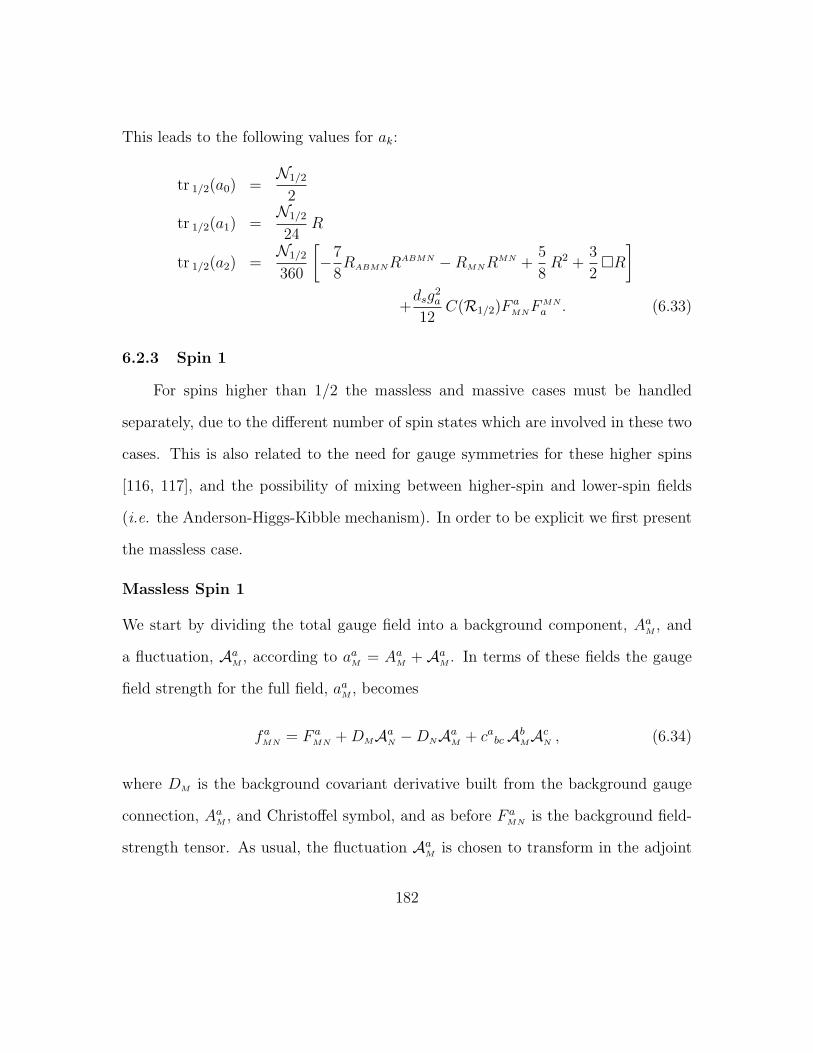
This leads to the following values for ak:

tr 1/2(a0) =N1/2

2

tr 1/2(a1) =N1/2

24R

tr 1/2(a2) =N1/2

360

[−7

8RABMNR

ABMN −RMNRMN +

5

8R2 +

3

2R

]+dsg

2a

12C(R1/2)F a

MNFMN

a . (6.33)

6.2.3 Spin 1

For spins higher than 1/2 the massless and massive cases must be handled

separately, due to the different number of spin states which are involved in these two

cases. This is also related to the need for gauge symmetries for these higher spins

[116, 117], and the possibility of mixing between higher-spin and lower-spin fields

(i.e. the Anderson-Higgs-Kibble mechanism). In order to be explicit we first present

the massless case.

Massless Spin 1

We start by dividing the total gauge field into a background component, AaM , and

a fluctuation, AaM , according to aaM = AaM + AaM . In terms of these fields the gauge

field strength for the full field, aaM , becomes

faMN = F aMN +DMAaN −DNAaM + cabcAbMAcN , (6.34)

where DM is the background covariant derivative built from the background gauge

connection, AaM , and Christoffel symbol, and as before F aMN is the background field-

strength tensor. As usual, the fluctuation AaM is chosen to transform in the adjoint

182

representation under background gauge transformations — and so (ta)bc = −icabc —

as well as transforming as a vector under background coordinate transformations.

It is convenient to fix the spin-1 gauge invariance using a background-covariant

gauge-averaging term,

e−1 L gfV = − 1

2ξ1

(DMAaM)2, (6.35)

where DM denotes the background-covariant derivative built from the background

gauge field and Christoffel symbols. Then expanding the gauge-field Lagrangian,

e−1 (LV + L gfV ) = −[

1

4faMNf

MN

a +1

2 ξ1

(DMAaM)2

], (6.36)

to second order in AaM and choosing the background-covariant Feynman gauge (ξ1 =

1), the part of the Lagrangian which is quadratic in the fluctuations, LA, becomes

e−1 LA = −1

2AM

a

[−gMNδ

ab − Y abMN + c ab

c F cMN

]AN

b , (6.37)

where as before [DM , DN ]AaN = Y abMN AN

b .

For a vector field the Lorentz generators are (JAB)CD = −i(δACδBD − δADδBC ), and

so we see that [DM , DN ]ANb = RMNAN

b − iF aMN(ta)

cb AN

c . The one-loop contribution

due to vector loops is then given by:

iΣV = −1

2log det

[∆M a

N b

]= −1

2log det

[− δMNδ

ab −RM

Nδab + 2iF cM

N(tc)ab

]. (6.38)

We can now see that XM aN b = −ηRM

Nδab + 2i(tc)

ab F

cMN , where η = ±1 is a useful

constant to include for later purposes. For the case considered here we see that

183

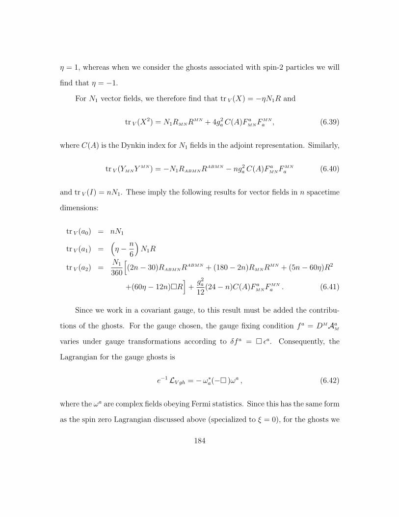
η = 1, whereas when we consider the ghosts associated with spin-2 particles we will

find that η = −1.

For N1 vector fields, we therefore find that tr V (X) = −ηN1R and

tr V (X2) = N1RMNRMN + 4g2

a C(A)F aMNF

MN

a , (6.39)

where C(A) is the Dynkin index for N1 fields in the adjoint representation. Similarly,

tr V (YMNYMN) = −N1RABMNR

ABMN − ng2a C(A)F a

MNFMN

a (6.40)

and tr V (I) = nN1. These imply the following results for vector fields in n spacetime

dimensions:

tr V (a0) = nN1

tr V (a1) =(η − n

6

)N1R

tr V (a2) =N1

360

[(2n− 30)RABMNR

ABMN + (180− 2n)RMNRMN + (5n− 60η)R2

+(60η − 12n)R]

+g2a

12(24− n)C(A)F a

MNFMN

a . (6.41)

Since we work in a covariant gauge, to this result must be added the contribu-

tions of the ghosts. For the gauge chosen, the gauge fixing condition fa = DMAaM

varies under gauge transformations according to δfa = εa. Consequently, the

Lagrangian for the gauge ghosts is

e−1 LV gh = −ω∗a(− )ωa , (6.42)

where the ωa are complex fields obeying Fermi statistics. Since this has the same form

as the spin zero Lagrangian discussed above (specialized to ξ = 0), for the ghosts we

184

may simply adopt the spin-0 results for the ak, with N0 → N1 and multiplied by an

overall factor of −2.

Adding the results for vector fields (η = +1) and ghosts gives the contribution

of physical spin-1 states. Thus, we obtain for massless spin-1 particles:

tr 1(a0) = N1(n− 2)

tr 1(a1) =N1

6(8− n)R

tr 1(a2) =N1

180

[(n− 17)RABMNR

ABMN + (92− n)RMNRMN

]+N1

72(n− 14)R2

+N1

30(7− n)R +

g2a

12(26− n)C(A)F a

MNFMN

a . (6.43)

Massive Spin 1

If the gauge symmetry is spontaneously broken by the expectation of a scalar field,

〈φi〉 = vi, then the previous discussion is complicated because the part of the La-

grangian quadratic in fluctuations acquires cross terms between the vector and scalar

fields of the form AaMta∂Mφ. These terms reflect the physical process whereby the

spin-1 particles acquire masses by absorbing the scalar fields through the Anderson-

Higgs-Kibble mechanism.

In this case the same analysis as above can be performed provided we average

over a more general gauge condition: fa = DMAaM + c v · taφ, with the constant c

chosen to remove the cross terms between AaM and ∂Mφ. This simply results in the

addition of the same mass matrix µ2 to the differential operator ∆ = −+X for the

vector fields and the ghost fields. This process also results in the would-be Goldstone

185

bosons (i.e. the scalar fields which mixed with the gauge fields) acquiring the same

mass matrix, µ2 as also appears in the vector-field and ghost actions [118, 119].

The upshot for massive spin-1 particles is therefore to add the result for N1

massless spin-1 particles to that of N1 massless scalar fields, with ξ = 0. This leads

to the following contributions if the mass µ2, is not included in X:

tr 1m(a0) = N1(n− 1)

tr 1m(a1) =N1

6(7− n)R

tr 1m(a2) =N1

180

[(n− 16)RABMNR

ABMN + (91− n)RMNRMN

]+N1

72(n− 13)R2

+N1

30(6− n)R +

g2a

12(25− n)C(A)F a

MNFMN

a . (6.44)

6.2.4 Antisymmetric Tensors

We next consider in detail the antisymmetric rank-2 gauge potential, BMN , which

appears in supergravity models. As before we first treat the massless case, and then

move on to massive particles. We also quote the results for massless antisymmet-

ric tensors of arbitrary rank, as taken from ref. [120, 121]. Since the calculations

in the subsequent sections parallel those for the spin-1 field, we omit the detailed

calculations from the main text and instead include these in appendix C.

Massless Antisymmetric Tensors

The appropriate Lagrangian for this field is

e−1 LB = − 1

12HMNPH

MNP , (6.45)

186

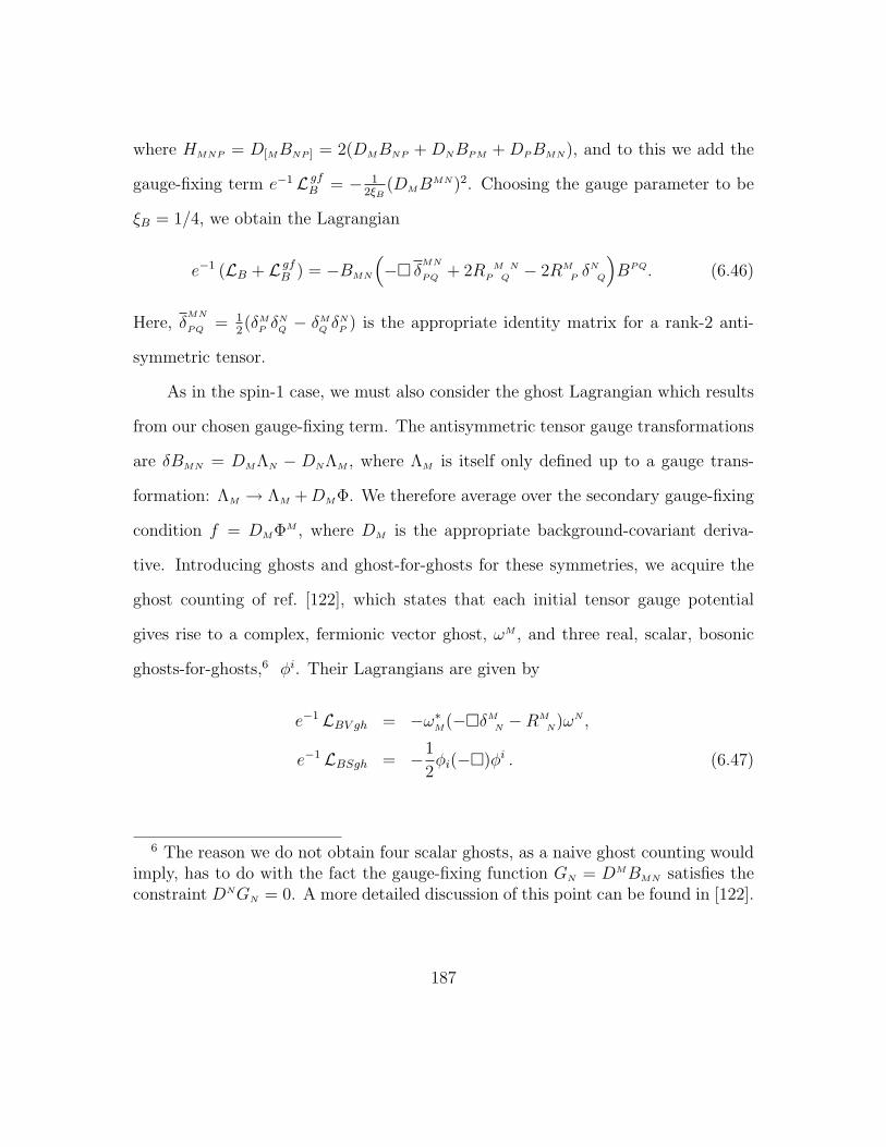
where HMNP = D[MBNP ] = 2(DMBNP + DNBPM + DPBMN), and to this we add the

gauge-fixing term e−1 L gfB = − 12ξB

(DMBMN)2. Choosing the gauge parameter to be

ξB = 1/4, we obtain the Lagrangian

e−1 (LB + L gfB ) = −BMN

(− δ

MN

PQ + 2R M N

P Q − 2RM

P δN

Q

)BPQ. (6.46)

Here, δMN

PQ = 12(δMP δ

NQ − δMQ δNP ) is the appropriate identity matrix for a rank-2 anti-

symmetric tensor.

As in the spin-1 case, we must also consider the ghost Lagrangian which results

from our chosen gauge-fixing term. The antisymmetric tensor gauge transformations

are δBMN = DMΛN − DNΛM , where ΛM is itself only defined up to a gauge trans-

formation: ΛM → ΛM +DMΦ. We therefore average over the secondary gauge-fixing

condition f = DMΦM , where DM is the appropriate background-covariant deriva-

tive. Introducing ghosts and ghost-for-ghosts for these symmetries, we acquire the

ghost counting of ref. [122], which states that each initial tensor gauge potential

gives rise to a complex, fermionic vector ghost, ωM , and three real, scalar, bosonic

ghosts-for-ghosts,6 φi. Their Lagrangians are given by

e−1 LBV gh = −ω∗M(−δMN −RM

N)ωN ,

e−1 LBSgh = −1

2φi(−)φi . (6.47)

6 The reason we do not obtain four scalar ghosts, as a naive ghost counting wouldimply, has to do with the fact the gauge-fixing function GN = DMBMN satisfies theconstraint DNGN = 0. A more detailed discussion of this point can be found in [122].

187

The contributions of the vector ghosts to ak is therefore obtained by replacing N1 →

−2Na in the result given above for vector fields (with η = +1). Similarly, the scalar

ghosts are obtained from the spin-0 result quoted above, with the replacements

N0 → 3Na and ξ → 0.

Summing the contribution of the rank-2 tensor and its ghosts leads to the follow-

ing expression for the physical massless particles associated with these antisymmetric

tensor fields:

tr a(a0) =Na

2(n− 2)(n− 3)

tr a(a1) = −Na

12(n2 − 17n+ 54)R

tr a(a2) =Na

360

[(n2 − 35n+ 306)RABMNR

ABMN − (n2 − 185n+ 1446)RMNRMN

]+Na

144(n2 − 29n+ 174)R2 − Na

60(n2 − 15n+ 46)R . (6.48)

Massive Particles

The particles associated with antisymmetric tensor fields can also acquire mass

through an Anderson-Higgs-Kibble mechanism, in which the antisymmetric tensor

particle ‘eats’ an ordinary gauge field, VM [123]. As before, a modification of the

gauge choice is required in this case in order not to have mixing terms of the form

BMN∂MVN . As we now show, the contribution of each massive tensor particle is given

by adding the above result for a massless particle to the result for an η = +1 massless

abelian — so with C(A) = 0 — gauge field (including its ghosts).

To demonstrate this explicitly, we start with the Lagrangian

e−1 LmB = − 1

12HMNPH

MNP − 1

4(VMN − 2mBMN)2, (6.49)

188

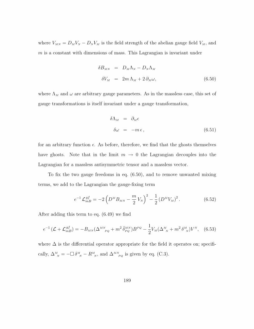
where VMN = DMVN −DNVM is the field strength of the abelian gauge field VM , and

m is a constant with dimensions of mass. This Lagrangian is invariant under

δBMN = DMΛN −DNΛM

δVM = 2mΛM + 2 ∂Mω, (6.50)

where ΛM and ω are arbitrary gauge parameters. As in the massless case, this set of

gauge transformations is itself invariant under a gauge transformation,

δΛM = ∂Mε

δω = −mε , (6.51)

for an arbitrary function ε. As before, therefore, we find that the ghosts themselves

have ghosts. Note that in the limit m → 0 the Lagrangian decouples into the

Lagrangian for a massless antisymmetric tensor and a massless vector.

To fix the two gauge freedoms in eq. (6.50), and to remove unwanted mixing

terms, we add to the Lagrangian the gauge-fixing term

e−1 L gfmB = −2(DMBMN −

m

2VN

)2

− 1

2(DMVM)2 . (6.52)

After adding this term to eq. (6.49) we find

e−1 (L+ L gfmB) = −BMN(∆MN

PQ +m2 δMN

PQ )BPQ − 1

2VM(∆M

N +m2 δMN)V N , (6.53)

where ∆ is the differential operator appropriate for the field it operates on; specifi-

cally, ∆MN = − δMN −RM

N , and ∆MNPQ is given by eq. (C.3).

189

The Lagrangian for the ghosts is obtained by varying the gauge-fixing conditions

appearing in eq. (6.52), and we thus find

LmBgh = −ξ∗N(−δNM +DMDN +m2δNM) ξM − ω∗(−)ω

−mξ∗MDMω +mω∗DMξ

M . (6.54)

Here, ξM and ω are the ghost fields associated with ΛM and ω, respectively. To fix

the gauge freedom implied by eq. (6.51), we add to the ghost Lagrangian the term

L gfmBgh = −(DMξM +mω)∗(DNξ

N +mω) (6.55)

and so we find

LmBgh + L gfmBgh = −ξ∗N[(− +m2)δNM +RN

M

]ξM − ω∗(− +m2)ω. (6.56)

Notice that the complex scalar ghost, ω, combines with the vector, VN , to form the

field content of a physical massless spin-1 particle.

The ghosts-for-ghosts Lagrangian is similarly obtained, and as in the massless

case we find three bosonic scalar ghosts-for-ghosts, with Lagrangian

LmBSgh = −1

2φi(− +m2)φi . (6.57)

Except for the presence of mass terms, the Lagrangian for a massive antisymmetric

tensor is therefore the sum of a massless spin-1 Lagrangian and a massless antisym-

metric tensor Lagrangian (including their ghosts). Thus, in calculating the ak for a

massive antisymmetric tensor, we simply need to add to the massless result given in

190

the previous section the result for a massless spin-1 field. It is important to empha-

size that such a sum — where we factor all mass terms out of X, as described in the

§ 6.1 — makes sense only because in the gauge we have chosen all particles share the

same mass.

The result of this sum, for massive rank-2 tensor fields in n spacetime dimensions,

is

tr am(a0) =Na

2(n− 2)(n− 1)

tr am(a1) = −Na

12(n2 − 15n+ 38)R

tr am(a2) =Na

360

[(n2 − 33n+ 272)RABMNR

ABMN − (n2 − 183n+ 1262)RMNRMN

]+Na

144(n2 − 27n+ 146)R2 − Na

60(n2 − 13n+ 32)R . (6.58)

Higher-Rank Antisymmetric Tensors

The result for a higher-rank massless skew-tensor gauge potential in n dimensions

has been worked out in a similar fashion to the above [120, 121]. This leads to the

following results for the first few Gilkey coefficients for a massless 3-form gauge field

(for n > 4 dimensions), specialized to Ricci-flat background geometries (RMN = 0):

tr 3a(a0) =N3a

3!(n− 2)(n− 3)(n− 4)

tr 3a(a1) = 0

tr 3a(a2) =N3a

1080(n3 − 54n2 + 971n− 4164)RABMNR

ABMN . (6.59)

191

The analogous results for a massless 4-form gauge field (in n > 5 Ricci-flat dimen-

sions) are given by:

tr 4a(a0) =N4a

4!(n− 2)(n− 3)(n− 4)(n− 5)

tr 4a(a1) = 0

tr 4a(a2) =N4a

4320(n4 − 74n3 + 2051n2 − 18634n+ 52680)RABMNR

ABMN .

(6.60)

These results for massive 1- and 2-forms suggest a short-cut for extending our

results to the case of a massive p-form for arbitrary p, since they show that the

Gilkey coefficients for a massive p-form are obtained by summing the contributions

of a massless (p − 1)-form to that of a massless p-form. It can also be readily seen

that the Gilkey coefficients for a massive spin-1 field are obtained by the replacement

n → (n + 1) in the massless formulae, and similarly for the antisymmetric 2-form.

One way to see why this should give the correct result is to reason as follows. It is

clear that (for a Minkowski-space background) a massless p-form in (n+1) dimensions

and a massive p-form in n dimensions share the same little group, SO(n − 1), and

transform in the same representation of this group. This connection can also be made

more explicit by dimensionally reducing an (n+1)-dimensional massless p-form on S1

to obtain a Kaluza-Klein tower of massive p-forms in the lower-dimensional theory.

Each massive field is thereby seen to contain the spin content of an n-dimensional

massless p- and (p − 1)-form. A final check on this reasoning can be had using

the results of ref. [120, 121], which show that the first few Gilkey coefficients for a

massless (n + 1)-dimensional p-form — and hence a massive n-dimensionsal p-form

192

— are the same as the sum of the coefficients for a massless p- and (p − 1)-form in

n dimensions.

6.2.5 Spin 3/2

Before proceeding with spin-3/2 and spin-2 particles, we first pause to es-

tablish a few of our supergravity conventions. Our starting point is the coupled

Einstein/Rarita-Schwinger system. We take the spin-2 field to be described by the

standard Einstein-Hilbert action, which in our conventions is

e−1 LEH = − 1

2κ2R, (6.61)

with κ2 = 8πGN . For the moment, we do not include a cosmological term; the

generalization of the massless and massive spin-3/2 particle to the case of a nonzero

cosmological constant is given in appendix D.

The spin-3/2 particle is described by a vector-spinor field, ψM , with a kinetic

term given by the Lagrangian

e−1 LV S = −1

2ψMΓMNPDNψP . (6.62)

As before, we use indices A,B, . . . for the tangent frame, M,N, . . . for world indices

and lower-case indices to label gauge-group generators. Conversion between tangent

and world indices is accomplished using the vielbein, e AM . Here, ΓABC = 1

6[ΓAΓBΓC +

· · · ] and ΓAB = 12[ΓA,ΓB] are normalized completely antisymmetric combinations of

gamma matrices.

The covariant derivative appearing in eq. (6.62) can involve background gauge

fields in addition to the Christoffel connection, but only if the corresponding gauge

193

symmetry does not commute with supersymmetry. Such transformations are partic-

ularly rich when there is more than one supersymmetry in the problem. Gravitini

cannot carry charges for internal symmetries which commute with supersymmetry,

because for these the gravitino must share the charge of the graviton, which is neutral

under all gauge transformations.

When there are no gauge fields in DMψN , it is straightforward to verify that the

combination LV S + LEH is invariant under the linearized supersymmetry transfor-

mations

δe A

M = −κ4ψMΓAε+ c.c. , δψM =

1

κDMε . (6.63)

When background gauge fields are present in DMψN , the combination LV S + LEH

varies into terms involving these gauge fields. These terms then cancel against vari-

ations of the gauge-field kinetic terms and with gauge-field-dependent terms in the

gravitino transformation law. This shows that gauge fields for symmetries which do

not commute with supersymmetry are special in that they are intimately related to

the gravitini by supersymmetry.

Massless Spin 3/2

In order to put the spin-3/2 Lagrangian into a form for which the general expressions

for the Gilkey coefficients apply, it is convenient to use the following gauge-averaging

term,

e−1 L gfV S = − 1

2 ξ3/2

(Γ · ψ) /D(Γ · ψ) . (6.64)

With this term, and after making the field redefinition ψM → ψM + AΓMΓ · ψ, we

find that the Lagrangian simplifies in the desired way when we make the following

194

choices for A and ξ3/2:

A =1

2− nand

1

ξ3/2

=2− n

4. (6.65)

These choices allow the vector-spinor Lagrangian to be written as

e−1 (LV S + L gfV S) = −1

2ψM /DψM , (6.66)

and so give the one-loop contribution

iΣ =1

2log det

[( /D)AB

]=

1

4log det

[(− /D2)AB

]. (6.67)

We next consider the contribution from the ghost fields. From the supersymme-

try transformation rules, we see that δ(Γ · ψ) = 1κ

/D ε and so there are two bosonic,

Faddeev-Popov spinor ghosts with the Lagrangian

e−1 LLV FPgh = −ωi /Dωi, (6.68)

where i = 1, 2 labels the two ghosts. Since this has the same form as the spin-

1/2 Lagrangian used earlier, eq. (6.30), the Faddeev-Popov ghost result for tr [ak] is

obtained by multiplying the massless spin-1/2 result by −2.

In addition to the Faddeev-Popov ghosts, there is also a bosonic, Nielsen-Kallosh

ghost [124, 125] coming from the use of the operator /D in the gauge-fixing La-

grangian, eq. (6.64). The Nielsen-Kallosh ghost Lagrangian is given by

e−1 LLV NKgh = −η /Dη . (6.69)

195

This ghost therefore has a contribution to tr [ak] given by −1 times the massless

spin-1/2 result.

Adding the results for the Faddeev-Popov and Nielsen-Kallosh ghosts to that of

the vector-spinor, we obtain the following results for the contribution to tr [ak] by

physical massless spin-3/2 states:

tr 3/2(a0) =N3/2

2(n− 3)

tr 3/2(a1) =N3/2

24(n− 3)R

tr 3/2(a2) =N3/2

360

[(30− 7

8(n− 3)

)RABMNR

ABMN − (n− 3)RMNRMN

+5

8(n− 3)R2 +

3

2(n− 3)R

]+dsg

2a

12(n− 3)C(R3/2)F a

MNFMN

a .

(6.70)

Massive Spin 3/2

A spin-3/2 state acquires a mass through the existence of an off-diagonal cou-

pling of the form χΓ·ψ with a spin-1/2 Goldstone fermion state, χ. Choosing a gauge

for which this term vanishes causes the super-Higgs mechanism to occur, through

which the spin-3/2 particle ‘eats’ the fermion χ. Although χ vanishes in a unitary

gauge, it remains in the theory in a covariant gauge much as does the would-be

Goldstone boson for the massive spin-1 case.

196

To show explicitly how this process occurs, we assume that the part of the

fermionic Lagrangian which is quadratic in the fluctuations has the general form7

e−1 LmV S = −ψMΓMNPDNψP − χ /Dχ−[ψ · Γ(a /D + b)χ+ c.c.

]−(c ψMD

Mχ+ c.c.)−m1/2 χχ− µ3/2 ψMψ

M

+m3/2ψMΓMNψN , (6.71)

where the parameters a, b, c, m1/2, m3/2, and µ 3/2 are constrained by demanding that

the action be invariant under linearized supersymmetry transformations. For sim-

plicity we assume these parameters to be real, although in general some or all of these

parameters may be complex, depending on whether the fermions are Majorana or

Weyl in the supergravity of interest. Requiring invariance under the supersymmetry

transformations

δψM =1

κDMε+ µΓMε and δχ = fε , (6.72)

then imposes the following constraints on the various parameters:

a = c = µ 3/2 = 0 b = κf f 2 = (n− 1)(n− 2)µ2

m1/2 = nκµ m3/2 = (n− 2)κµ . (6.73)

This leaves one free parameter which we can take to be µ, f , or b.

7 We follow here the approach of refs. [126, 127, 128] to identify the form of thesecouplings to quadratic order in a model-independent way.

197

With these choices, the variation of the gravitino/goldstino Lagrangian is

e−1 δLmV S =1

2κGMNψMΓNε+ c.c., (6.74)

where GMN = RMN − 12RgMN is the Einstein tensor. This term is cancelled in

the usual way by the variation of the Einstein-Hilbert action under the graviton

transformation

δe A

M = −κ4ψMΓAε+ c.c. (6.75)

To this Lagrangian we add the gauge-fixing term

1

eL gfmV S = −F ( /D + γ)F, (6.76)

where

F = αΓ · ψ + βχ. (6.77)

The constants α, β, and γ are chosen to ensure that the gauge-fixed Lagrangian has

the form

e−1 (LmV S + L gfmV S) = −ψ′M( /D +m′3/2)ψ′M − χ′( /D +m′1/2)χ′ (6.78)

where ψ′M and χ′ are given by

χ′ = Aχ+B Γ · ψ and ψ′M = ψM + C ΓMΓ · ψ +DΓMχ , (6.79)

where we again take the parameters A, B, C, and D to be real for simplicity. Note

that the transformation of ψM is non-singular provided C 6= −1/n. Using eq. (6.79)

to evaluate the right-hand side of eq. (6.78) while using eqs. (6.71), (6.73), and (6.76)

198

to evaluate the left-hand side, leads to the conditions

A =

(n− 1

n− 2

)1/2

, B = C = −1

2, D = 0, m′3/2 = m′1/2 = (n− 2)κµ,

α = −1

2

√n− 1, β =

1√n− 2

, γ = −(n− 2)κµ. (6.80)

The ghost action consists of a Nielsen-Kallosh ghost, with Lagrangian

e−1 LmV SNK = −ω( /D + γ)ω, (6.81)

as well as two Faddeev-Popov ghosts, with Lagrangian

e−1 LmV SFP = −ξi[

/D + (n− 2)κµ]ξi , (6.82)

where i = 1, 2 labels the two ghosts. Dropping the primes, and defining m =

(n− 2)κµ, the complete Lagrangian, eqs. (6.78), (6.81) and (6.82), becomes

e−1 Lm3/2 = −ψM( /D +m)ψM − χ( /D +m)χ− ω( /D −m)ω − ξi( /D +m)ξi . (6.83)

Since the heat-kernel coefficients are even under m→ −m, we see from this that

ak for a massive gravitino are given by the sum of the corresponding coefficients for

a massless gravitino (including ghosts) plus those of a massless fermion. Summing

the massive spin-1/2 result, eq. (6.33), with the spin-3/2 result, eq. (6.70), we obtain

199

the following Gilkey coefficients for a massive spin-3/2 particle

trm3/2(a0) =N3/2

2(n− 2)

trm3/2(a1) =N3/2

24(n− 2)R

trm3/2(a2) =N3/2

360

[(30− 7

8(n− 2)

)RABMNR

ABMN − (n− 2)RMNRMN

+5

8(n− 2)R2 +

3

2(n− 2)R

]+g2a

12(n− 2)dsC(R3/2)F a

MNFMN

a .

(6.84)

6.2.6 Spin 2

Finally, we turn to spin-2 particles. In order to maximize the utility of this

section, we do so for the case where the Lagrangian includes a cosmological constant,

as is typically true for non-supersymmetric theories (and for supersymmetric theories

in four dimensions), and so start with the following action

e−1 LEH = − 1

2κ2(R + 2Λ) . (6.85)

For situations where Λ represents the value of a scalar potential, V , evaluated at the

classical background, we see from the above that Λ = +κ2 V .

Although it is usually true that only a single spin-2 particle is massless in any

given model, we include a parameter N2 which counts the massive spin-2 states. We

do so because there is typically more than one massive spin-2 state in the models of

interest, typically arising as part of a Kaluza-Klein tower or as excited string modes.

200

Massless Spin 2

The Lagrangian for a massless rank-two symmetric field is the Einstein-Hilbert ac-

tion, eq. (6.85). As usual we write the metric as gMN + 2κhMN , where gMN is the

background metric and hMN are the fluctuations. Expanding to quadratic order in

these fluctuations, and adding the gauge-fixing term

1

eL gfEH = −

(DMhMN −

1

2DNh

M

M

)2

, (6.86)

we obtain the standard result [129]

1

e(LEH + LgfEH) =

1

2hMN

[hMN + (R + 2Λ)hMN − (hMAR

A

N + hNARA

M )

−2RMANBhAB

]+ hMNRMNh−

1

4h[h+ (R + 2Λ)h

],

(6.87)

where h = gMNhMN .

It is useful to try to decouple the scalar, h, from the traceless symmetric tensor

φMN = hMN − 1nh gMN , in this expression. In terms of these variables the Lagrangian

is

1

e(LEH + L gfEH) =

1

2φMN

[φMN + (R + 2Λ)φMN − (φMAR

A

N + φNARA

M )

−2RMANBφAB

]+

(n− 4

n

)φMNRMN h

−(n− 2

4n

)[hh+

(n− 4

n

)Rh2 + 2Λh2

], (6.88)

which shows that these fields decouple in four dimensions, and in arbitrary dimen-

sions if we make the assumption that the background metric is an Einstein space:

201

RMN = 1nRgMN . It is straightforward to consider the case when this mixing term

does not vanish, and we do so at the end of the calculation. In the interim, however,

we ignore this term.

Canonically normalizing the scalar mode by taking φ = [(n − 2)/(2n)]1/2h, we

arrive at the desired expression:

1

e(LEH + L gfEH) = −1

2φMN

[− δABMN + 2R A B

M N + (RA

MδB

N +RA

NδB

M)

−(R + 2Λ)δABMN

]φAB −

1

2φ

[ +

(n− 4

n

)R + 2Λ

]φ+ · · · ,

(6.89)

where δMNAB = 1

2(δMA δ

NB +δMB δ

NA )− 1

ngMNgAB is the unit matrix appropriate for a traceless

symmetric tensor, and the ellipsis denotes the mixing term. Notice the presence of

the well-known ‘wrong’ sign for the kinetic term of the scalar mode φ. We may now

separately compute the contributions of φ and φMN to the heat-kernel coefficients,

ak (see appendix C for details of the φMN calculation).

The scalar part of the spin-2 Lagrangian is given by

1

eLEHs =

1

2φ

[−−

(n− 4

n

)R− 2Λ

]φ, (6.90)

which, apart from an overall sign, has the same form as eq. (6.27) if we make the sub-

stitution ξR→ −(n−4n

)R−2Λ. Since the overall sign of ∆ contributes a background-

field-independent phase to the action which is cancelled by a similar contribution

from the ghost action (see below), we may ignore it for the present purposes. With

these comments in mind, we may then use the previous results for spin-0 fields to

compute the contribution of φ to the Gilkey coefficients, ak.

202

We now consider the ghosts for the graviton field. Since the gauge-fixing term

is fN = DMhMN − 12DNh, and the gauge transformations are δhMN = DMξN +DNξM ,

we find the transformation property

δfN = ξN −RM

N ξM , (6.91)

leading to a complex, fermionic, vector ghost ωM with Lagrangian

e−1 L = −ω∗M(−δMN +RM

N )ωN . (6.92)

The contribution of the vector ghost to the Gilkey coefficients is therefore obtained

by multiplying the results found earlier for the real spin-1 field by an overall factor

of −2 (and using the choice η = −1 in eq. (6.41)).

Finally, we return to the issue of the mixing-term between the symmetric-

traceless and the trace components of the metric. Using the symmetries of φMN ,

this mixing term can be written as 2ZMNφMN φ, where

ZMN =n− 4

2n

√2n

n− 2

(RMN −

1

ngMNR

). (6.93)

The effect of this term can be included by adding an off-diagonal term to the matrix

X of the field Φ = (φMN , φ)T . Omitting indices, we haveXsymtr Z

Z Xtr

where Xsymtr corresponds to the mass matrix for φMN , and Xtr the mass matrix for

φ. Note that since the Gilkey coefficients only contain traces of polynomials of X,

the effect of this mixing first occurs in the term Tr (X2). It is easy to calculate now

203

that

Tr (X2) = Tr (X2)|Z=0 +n− 4

n2(n− 2)

(nRMNR

MN −R2). (6.94)

Collecting all these results, we thus obtain the first few Gilkey coefficients for

the massless graviton in n dimensions:

tr 2(a0) =N2

2n(n− 3)

tr 2(a1) = N2

[1

12(5n2 − 3n+ 24)R + n(n+ 1)Λ

]tr 2(a2) = N2

[1

360(n2 − 33n+ 540)RABMNR

ABMN

− 1

360n(n− 2)(n4 − 185n3 + 1086n2 + 4140n− 10800)RMNR

MN

+1

144n2(n− 2)(25n5 − 149n4 − 48n2 + 2232n− 4320)R2

+1

30(2n2 − n+ 10)R +

n

6(5n− 7)ΛR + n(n+ 1)Λ2

]. (6.95)

Massive Spin 2

We next derive the Lagrangian for the massive graviton. In order to do so we

require an expression for the quadratic part of the massive spin-2 Lagrangian, such

as might be obtained from a Kaluza-Klein reduction or as a massive string mode.

To keep the analysis as background-independent as possible, we work with the most

general such action for which the spin-2 state acquires its mass by mixing with the

appropriate Goldstone field, as in the Anderson-Higgs-Kibble mechanism. We believe

that by making this requirement we capture quite generally the contributions of the

massive spin-2 states which arise in dimensional reduction and as heavy string modes

[130, 131].

204

We start, therefore, with the Lagrangian

e−1 LmEH = e−1 LEH −1

4FMNF

MN − ahMNDMVN − bV MDMh

−cRMNVMVN −1

2m2

1 VMVM − 1

2m2

2 hMNhMN − 1

2µ2

2 h2 , (6.96)

where the coefficients a, b, c, m1, m2 and µ2 are to be determined by demanding the

presence of a non-linearly realized gauge symmetry (which would correspond to the

diffeomorphisms which do not preserve the background geometry within the Kaluza-

Klein context). FMN is the field strength DMVN −DNVM , where we take VM to have

the spin content of a massive spin-1 particle. From the previous sections we see that

this should consist of a specific combination of a massless vector field, AM , and a

would-be Goldstone scalar, σ. Accordingly, we make the definition

VM = AM + pDMσ , (6.97)

where the coefficient p is also to be determined in what follows. Notice that, as

defined, any Lagrangian built from the vector field VM automatically has the gauge

invariance

δAM = DMε and δσ = −1

pε. (6.98)

If we desire we may use unitary gauge for this symmetry to remove σ completely

from the theory, however this is not a convenient gauge for our purposes and so in

what follows we instead gauge-fix using a more convenient covariant gauge.

205

In order to implement the underlying gauge invariance which any such a spin-2

field must manifest we ask the above Lagrangian to be invariant under the usual spin-

2 gauge transformation δhMN = DMξN +DNξM , supplemented by the Goldstone-type

transformation δVM = fξM . This leads to the following Lagrangian8

e−1 LmEH = e−1 LEH −1

4FMNF

MN + f hMNDMVN + f V MDMh

−RMNVMVN −1

4f 2 hMNh

MN +1

4f 2 h2 , (6.99)

corresponding to the choices

a = b = −f, c = 1,

m1 = 0,

and m22 = −µ2

2 =f 2

2. (6.100)

We now fix the two gauge freedoms of this action in such a way as to remove

the mixings between the various fields having differing spins. To do so we take for

the spin-2 gauge-fixing Lagrangian

e−1 L gfmEH2 = −(fN −

1

2fVN

)2

, (6.101)

8 As a check on this result, we note that by choosing the gauge where VM = 0, werecover the Pauli-Fierz Lagrangian of massive gravity [132]. Also, in flat space, thisresult agrees (after a suitable field redefinition) with the one given in [133].

206

where f is the parameter appearing in the Lagrangian (6.99), and as before fN is

defined as fN = DMhMN− 12DNh. This gauge choice removes the hMNDMVN term from

the action and introduces a mass term, m, for the vector field, VM , with m2 = 12f 2.

To fix the other gauge freedom, eq. (6.98), we add the following gauge-fixing

term

e−1 L gfmEH1 = −1

2(DMA

M + λh+ r σ)2, (6.102)

with λ and r being parameters which are chosen to remove the remaining vector-

gravity mixing terms in the quadratic action. In order to to simplify the analysis, we

specialize to the case where the background spacetime is an Einstein space, which

we also take to be a solution to the Einstein equations of the form GMN −ΛgMN = 0,

or RMN = −[2Λ/(n − 2)] gMN . Using this we see that the removal of cross terms

between AM , hMN , and σ requires the choices

λ = −f2, and r = p q2, (6.103)

where q2 is defined as

q2 = m2 − 4Λ

n− 2, (6.104)

since in this case the gauge-fixed Lagrangian can be written as

LmEH + L gfmEH1 + L gfmEH2 = LmEH0 + LmEH1 + LmEH2 , (6.105)

with the decoupled Lagrangians, LmEH0, LmEH1, and LmEH2, defined as follows.

207

LmEH2 denotes the φMN Lagrangian, which takes the form

e−1 LmEH2 =1

eLEH − fNfN −

1

4f 2hMNh

MN +1

8f 2h2

= −1

2φMN

(∆MN

PQ +m2δMN

PQ

)φPQ

+

(n− 2

4n

)h

(− +m2 +

1

n(4− n)R− 2Λ

)h

+

(n− 4

n

)RMNφ

MNh

= −1

2φMN

(∆MN

PQ +m2δMN

PQ

)φPQ

+1

2φ

(− +m2 − 4Λ

n− 2

)φ, (6.106)

where φ, φMN , δMNAB and ∆MN

PQ are as defined above for the massless spin-2 case.

The mass m is related to the symmetry-breaking parameter f by m2 = 12f 2.

We similarly find the following vector Lagrangian, LmEH1:

e−1 LmEH1 = −1

4FMNF

MN − 1

2(DMAM)2 −RMNAMAN −

1

2m2AMA

M

= −1

2AM

[(− +m2) δMN +RM

N

]AN , (6.107)

where m is the same as for φMN .

Finally, the part of the quadratic action depending on σ is

e−1 LmEH0 =1

2

[(pr)σσ − (pf)σh− (r2)σ2 + (fr)hσ

], (6.108)

which contains terms which mix σ and h. However, since p is as yet unspecified we

may choose its value to remove these cross terms. This may be done by choosing

208

p = −f/(4q2) and making the field redefinition σ =√

2m4q

(σ+2h), after which we find

e−1 LmEH0 = −1

2σ

(− +m2 − 4Λ

n− 2

)σ

+

(m2

4q2

)h

(− +m2 − 4Λ

n− 2

)h. (6.109)

Notice that in this form the last term in LmEH0 (involving h) has the same form as the

last term in LmEH2, and so these can both be combined into LmEH2 by appropriately

rescaling the scalar φ. Once this is done, and dropping the tilde on σ, the remaining

term becomes

e−1 LmEH0 = −1

2σ

[− +m2 − 4Λ

n− 2

]σ. (6.110)

Finally, the action for the ghosts can be easily calculated from the gauge-fixing

conditions. The spin-2 gauge-fixing term introduces a complex, fermionic, vector

ghost with Lagrangian

e−1 LmEHV gh = −ω∗M[(− +m2) δMN +RM

N

]ωN . (6.111)

Similarly, the spin-1 gauge-fixing term introduces a complex scalar ghost with La-

grangian

e−1 LmEHSgh = −ω∗(− +m2 − 4Λ

n− 2

)ω. (6.112)

The complete Lagrangian, including all ghosts, for the massive graviton is thus

the sum

Lm2 = LmEH0 + LmEH1 + LmEH2 + LmEHSgh + LmEHV gh. (6.113)

209

We are now in a position to assemble the results for ak. To this end, notice that

all fields have been decoupled in the kinetic terms and all now have the same mass,

m2 = 12f 2. This allows us to sum the separate contributions to ak from each of these

fields. It is also interesting to note that the scalar fields h, σ and the complex scalar

ghost all have precisely the same Lagrangian, and so their net effect is to completely

cancel one another in the one-loop action. Similarly, the vector boson AM and the

complex vector ghost also share the same Lagrangian, and so for our purposes these

two together contribute the equivalent of one real vector ghost.

In summary, the one-loop divergences for the massive graviton are given by the

sum of the divergences of a symmetric traceless field and one real vector ghost (for

which η = −1). Thus, we find

tr 2m(a0) =N2

2(n+ 1)(n− 2)

tr 2m(a1) = −N2

[(6− n)(n+ 4)(n+ 1)Λ

6(n− 2)

]tr 2m(a2) = N2

[1

360(n2 − 31n+ 508)RABMNR

ABMN

+(5n4 − 7n3 − 248n2 − 596n− 1440)Λ2

180(n− 2)2

](6.114)

for n-dimensional massive gravitons on background metrics satisfying GMN−ΛgMN =

0.

6.3 Supergravity Models

In supergravity theories the ultraviolet sensitivity of the low-energy theory is

often weaker than in non-supersymmetric models. This weaker sensitivity arises due

210

to cancellations between the effects of bosons and fermions in loops. The purpose

of this section is to illustrate the utility of the previous section’s results by using

them to exhibit this cancellation explicitly for supergravities in various dimensions.

Some of the results we obtain — particularly those for massless particles in higher-

dimensional supergravities — are computed elsewhere, and we use the agreement

between these earlier calculations and our results as a check on the validity of our

computations.

We proceed by summing the above expressions over the particles appearing in

the appropriate supermultiplets. The result for the ultraviolet-sensitive part of the

one-loop action obtained by integrating out a supermultiplet is given by

ΣUV =1

2

(1

4π

)n/2 ∫dnx√−g

[n/2]∑k=0

∑p

(−)F (p)mn−2kp Γ(k − n/2) tr p[ak] , (6.115)

where the sum on p runs over the elements of a supermultiplet. As is clear from

this expression, it is the weighted sum∑

p(−)F (p) mn−2kp tr p[ak] which is of interest

in supersymmetric theories.

In Minkowski space the strongest suppression of UV sensitivity arises when

supersymmetry is unbroken, in which case all members of a supermultiplet share the

same mass (so that mp = m for all p). In this case, eq. (6.115) can be written as

ΣUV =1

2

(1

4π

)n/2 ∫dnx√−g

[n/2]∑k=0

mn−2k Γ(k − n/2) Tr [ak] , (6.116)

where

Tr [ak] ≡∑p

(−)F (p) tr p[ak] (6.117)

211

is the relevant combination of heat-kernel coefficients for a supermultiplet. Since

tr [a0] simply counts the spin states of the corresponding particle type, the cancella-

tion of the leading UV sensitivity occurs for a mass-degenerate supermultiplet simply

because each supermultiplet contains equal numbers of bosons and fermions:

Tr [a0] =∑p

(−)F (p)tr p[a0] = NB −NF = 0 . (6.118)

This ensures the absence of a dependence of the form mn in ΣUV .

The story is more complicated when there is a nonzero cosmological constant,

and this is because mass itself is more delicate to define in de Sitter or anti-de Sitter

spacetimes. For Minkowski space mass can be defined for particle states as a Casimir

invariant of the Poincare group, but this definition is no longer appropriate when

Λ is nonzero because Poincare transformations are then not the relevant spacetime

isometries. Rather, for de Sitter space the relevant isometry group in four dimensions

is SO(4, 1), while the isometries of anti-de Sitter space fill out the group SO(3, 2). For

these geometries it only makes sense to inquire about the implications of unbroken

supersymmetry for the anti-de Sitter case. This is because supersymmetry is always

broken in de Sitter spacetime, whereas there is a supersymmetric generalization of

SO(3, 2) for which one can find particle supermultiplets which represent the unbroken

supersymmetry.

In our previous calculations of the Gilkey coefficients we have defined m2 to be

that piece in the operator (− + X) which is a constant for arbitrary background

212

fields.9 We nevertheless must still grapple with the above ambiguities as to the

meaning of mass in de Sitter and anti-de Sitter spacetimes, due to the freedom of

absorbing into m2 contributions coming from the background curvature for constant-

curvature spacetimes. One can try to restrict this freedom by demanding massless-

ness to correspond to conformal invariance or (for higher-spin fields) to unbroken

gauge invariance, bearing in mind that these choices need not imply propagation

along the light cone [134].

The upshot of this discussion is that it need not be true that all of the particles

within a supermultiplet share the same mass even when working about a supersym-

metric AdS background. In such cases one cannot pull a common mass out of the

sum over particles within a supermultiplet, as was done in going from eq. (6.115) to

eq. (6.116).

To see this concretely, consider the specific example of a Wess-Zumino multiplet

in n = 4 spacetime dimensions expanded about a supersymmetric AdS background.

Such a multiplet consists of a scalar, pseudoscalar, and spinor field: (S, P, χ), and tak-

ing the scalar and pseudoscalar to have a conformal coupling parameter, ξ = −1/6,

their mass terms can be written as m2S = m2 − δm2, m2

P = m2 + δm2 and m2χ = m2.

Unbroken supersymmetry implies that these mass terms are related to one another

by m2 = −µ2Λ/12 and δm2 = −µΛ/6, where Λ is the AdS cosmological constant and

µ is a dimensionless parameter which classifies the massive supersymmetric particle

9 This statement requires appropriate modification in the case of spin 2, where weinclude a cosmological constant term in the Lagrangian.

213

representations. In this case, we find

∑p

(−)F (p)m4p tr p[a0] = m4

S tr S[a0] +m4P tr P [a0]−m4

χ tr χ[a0] = 2 δm4 =µ2Λ2

18∑p

(−)F (p)m2p tr p[a1] = m2

S tr S[a1] +m2P tr P [a1]−m2

χ tr χ[a1] = +2m2 Λ

3= −µ

2Λ2

18∑p

(−)F (p)m0p tr p[a2] = tr S[a2] + tr P [a2]− tr χ[a2] =

R2MNPQ

48− Λ2

9. (6.119)

The above complication keeps us from quoting general expressions for the sum

of the Gilkey coefficients over arbitrary supermultiplets in general dimensions, since

for AdS backgrounds these must be computed with the specific dependence of the

relevant masses on Λ. Notice however that the last expression in eq. (6.119) contains

no dependence on the individual particle masses (since tr p[a2] is multiplied by m0p =

1). Terms which are only present in the mass invariant piece of ΣUV , such as R2MNPQ

and F 2MN , can be calculated once and for all in a model-independent way because

their coefficients do not depend on the details of the particle masses involved.

As can be seen from the above example, however, calculating the complete an-

swer for ΣUV is not difficult once the individual particle masses are known. Similar

considerations hold for dimensions other than four, with some terms in ΣUV be-

ing mass independent and others requiring more detailed knowledge of the particle

spectrum about a given background.

6.4 Application to Ricci Flat Backgrounds in 6D

We now apply the previous results to the case where the background spacetime

is Ricci flat, satisfying RMN = 0. Since we are particularly interested in the UV

sensitivity of supersymmetric theories in six dimensions, we will need to calculate

214

Table 6–1: Results for massless particles in six dimensions, including ghost contri-butions and specialized to Ricci-flat background metrics. Note that the boson fieldsin this table are real and the fermion fields are 6D symplectic-Weyl spinors.

Field (−)F Tr [a0] (−)F Tr [a1] (−)F 720 Tr [a2] (−)F 45360 Tr [a3]φ 1 0 4R 2

ABMN −17 I1 + 28 I2

ψ −2 0 7R 2ABMN −29 I1 + 70 I2

AM 4 0 −44R 2ABMN 184 I1 − 392 I2

AMN 6 0 264R 2ABMN −7158 I1 + 14280 I2

ψM −6 0 −219R 2ABMN −591 I1 + 1218 I2

gMN 9 0 756R 2ABMN 8919 I1 − 17892 I2

the Gilkey coefficient a3 for the various spin fields. Fortunately, this is a matter of

simply plugging in our previous results into the the equation for a3, eq. (C.2). To

simplify the equations to come, we make use of the following result for a Ricci flat

space (we neglect total derivatives)

DERABCDDERABCD = −I1 − 4I2, (6.120)

where I1 and I2 are defined as

I1 = RABCDRAB

EFRCDEF

I2 = RABCDRA C

E FRBEDF . (6.121)

It should be noted that the integrand of the Euler number, χ, in 6 dimensions is

proportional to the combination −I1 + 2 I2. We now summarize the results of this

calculation for spin 0 through to spin 2. In the following formulae, N counts the

number of fields of a given spin. Tables (6–1) and (6–2) summarize the results

which these calculations imply respectively for massless and massive particles in 6

dimensions.

215

Table 6–2: Results for massive particles in six dimensions, specialized to Ricci-flatbackgrounds. Note that in this table the bosonic fields are real and the spinors aresymplectic, but not Weyl.

Multiplet (−)F Tr [a0] (−)F Tr [a1] (−)F 360 Tr [a2] (−)F 45360 Tr [a3]φ 1 0 2R 2

ABMN −17 I1 + 28 I2

ψ −4 0 7R 2ABMN −58 I1 + 140 I2

AM 5 0 −20R 2ABMN 167 I1 − 364 I2

AMN 10 0 110R 2ABMN −6974 I1 + 13888 I2

ψM −16 0 −212R 2ABMN −1240 I1 + 2576 I2

gMN 14 0 358R 2ABMN 9086 I1 − 18256 I2

6.4.1 Supersymmetric Multiplets

The next few sections record the analogous result for the coefficients a0 through

a3 once summed over the particles within various 6D supermultiplets, under the as-

sumption that all elements of the supermultiplet have the same 6D mass. Notice that

our discussion of the equivalence between performing the sum over the UV sensitive

part of the 4D contribution of each KK mode and the UV sensitivity as computed

using the full 6D fields shows that the assumption of equal masses within a 6D

supermultiplet relies only on there being unbroken (2, 0) supersymmetry at the high-

energy scale, M , appropriate to the compactification from higher dimensions down

to 6D. Provided that M mKK ∼ 1/r, this assumption does not require that some

supersymmetry remains unbroken below the scale of the KK masses encountered in

the compactification from 6D down to 4D.

Massless 6D Supermultiplets

We first summarize the particle content of the simplest 6D supermultiplets,

starting first with massless multiplets and then moving on to massive multiplets.

Our discussion follows that of ref. [135].

216

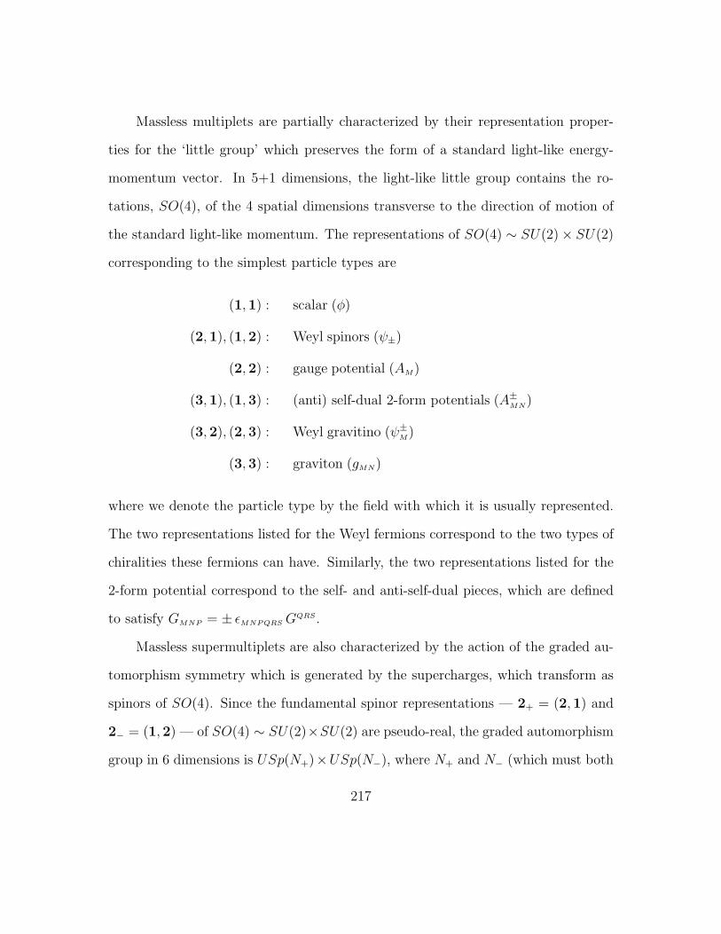
Massless multiplets are partially characterized by their representation proper-

ties for the ‘little group’ which preserves the form of a standard light-like energy-

momentum vector. In 5+1 dimensions, the light-like little group contains the ro-

tations, SO(4), of the 4 spatial dimensions transverse to the direction of motion of

the standard light-like momentum. The representations of SO(4) ∼ SU(2)× SU(2)

corresponding to the simplest particle types are

(1,1) : scalar (φ)

(2,1), (1,2) : Weyl spinors (ψ±)

(2,2) : gauge potential (AM)

(3,1), (1,3) : (anti) self-dual 2-form potentials (A±MN)

(3,2), (2,3) : Weyl gravitino (ψ±M)

(3,3) : graviton (gMN)

where we denote the particle type by the field with which it is usually represented.

The two representations listed for the Weyl fermions correspond to the two types of

chiralities these fermions can have. Similarly, the two representations listed for the

2-form potential correspond to the self- and anti-self-dual pieces, which are defined

to satisfy GMNP = ± εMNPQRS GQRS.

Massless supermultiplets are also characterized by the action of the graded au-

tomorphism symmetry which is generated by the supercharges, which transform as

spinors of SO(4). Since the fundamental spinor representations — 2+ = (2,1) and

2− = (1,2) — of SO(4) ∼ SU(2)×SU(2) are pseudo-real, the graded automorphism

group in 6 dimensions is USp(N+)×USp(N−), where N+ and N− (which must both

217

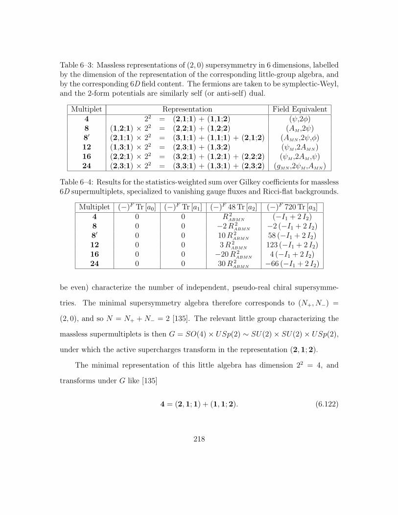
Table 6–3: Massless representations of (2, 0) supersymmetry in 6 dimensions, labelledby the dimension of the representation of the corresponding little-group algebra, andby the corresponding 6D field content. The fermions are taken to be symplectic-Weyl,and the 2-form potentials are similarly self (or anti-self) dual.

Multiplet Representation Field Equivalent4 22 = (2,1;1) + (1,1;2) (ψ,2φ)8 (1,2;1) × 22 = (2,2;1) + (1,2;2) (AM ,2ψ)8′ (2,1;1) × 22 = (3,1;1) + (1,1;1) + (2,1;2) (AMN ,2ψ,φ)12 (1,3;1) × 22 = (2,3;1) + (1,3;2) (ψM ,2AMN)16 (2,2;1) × 22 = (3,2;1) + (1,2;1) + (2,2;2) (ψM ,2AM ,ψ)24 (2,3;1) × 22 = (3,3;1) + (1,3;1) + (2,3;2) (gMN ,2ψM ,AMN)

Table 6–4: Results for the statistics-weighted sum over Gilkey coefficients for massless6D supermultiplets, specialized to vanishing gauge fluxes and Ricci-flat backgrounds.

Multiplet (−)F Tr [a0] (−)F Tr [a1] (−)F 48 Tr [a2] (−)F 720 Tr [a3]4 0 0 R 2

ABMN (−I1 + 2 I2)8 0 0 −2R 2

ABMN −2 (−I1 + 2 I2)8′ 0 0 10R 2

ABMN 58 (−I1 + 2 I2)12 0 0 3R 2

ABMN 123 (−I1 + 2 I2)16 0 0 −20R 2

ABMN 4 (−I1 + 2 I2)24 0 0 30R 2

ABMN −66 (−I1 + 2 I2)

be even) characterize the number of independent, pseudo-real chiral supersymme-

tries. The minimal supersymmetry algebra therefore corresponds to (N+, N−) =

(2, 0), and so N = N+ + N− = 2 [135]. The relevant little group characterizing the

massless supermultiplets is then G = SO(4)× USp(2) ∼ SU(2)× SU(2)× USp(2),

under which the active supercharges transform in the representation (2,1; 2).

The minimal representation of this little algebra has dimension 22 = 4, and

transforms under G like [135]

4 = (2,1; 1) + (1,1; 2). (6.122)

218

This consists of 2 real (1 complex) scalars and a single symplectic-Weyl fermion, and

so consists of 2 bosonic and 2 fermionic states.

Higher-dimensional representations may be obtained from this minimal one by

taking direct products of it with an irreducible representation of the bosonic part of

the little group. Table (6–3) lists some possible representations which are obtained

in this way, including the hyper-multiplet (4), gauge multiplet (8), tensor multiplet

(8′), two types of gravitino multiplet (12, 16) and the graviton multiplet (24). To

derive the results in this table, we use the standard results for SU(2): 2×2 = 1+3,

2× 3 = 2 + 4 and 2× 4 = 3 + 5.

We may now sum the previous expressions for the Gilkey coefficients over the

particle content of these massless 6D supermultiplets. The results obtained for

Tr sm[ak] =∑

p∈sm(−)F (p) Tr p[ak] if the particles all share the same mass are sum-

marized in table (6–4). Notice that the resulting expressions for Tr sm[a3] are pro-

portional to the combination −I1 + 2I2 which gives the Euler number density for

compact 6D manifolds.

Massive 6D supermultiplets

The massive representations of (2, 0) 6D supersymmetry are found in a similar

manner, except in this case the little group for the time-like energy-momentum vector

appropriate to massive fields is SO(5). The particle types and fields corresponding

219

Table 6–5: Massive representations of (2, 0) supersymmetry in six dimensions, la-belled by their dimension. Note that the fermions are not chiral and the 2-formpotentials are not self-dual or antiself-dual.

Mult. Representation Field Equivalent16m 24 = (5,1) + (1,3) + (4,2) (AmM ,2ψm,3φm)64m (4,1) × 24 = (16,1) + (4,1) + (4,3) (ψmM ,2AmMN ,2AmM ,4ψm,2φm)

+(10,2) + (5,2) + (1,2)80m (5,1) × 24 = (14,1) + (10,1) + (1,1) (gmMN ,2ψmM ,AmMN ,3AmM ,2ψm,φm)

+ (5,3) + (16,2) + (4,2)

to the representations of SO(5) are as follows:

1 : massive scalar (φm)

4 : massive spinor (ψm)

5 : massive gauge potential (AmM)

10 : massive 2-form (AmMN)

16 : massive gravitino (ψmM )

14 : massive graviton (gmMN) .

The little algebra for the supersymmetry representations is therefore SO(5) ×

USp(2). The irreducible spinor representations of SO(5) are not chiral, and are 4-

dimensional, and so the number of supercharges doubles in going from light-like to

time-like representations.10 It follows that the dimensionality of the minimal repre-

sentation is the square of what it was in the light-like situation: 24 = 16, with the

10 We assume here vanishing central charges — and so no ‘short’ multiplets.

220

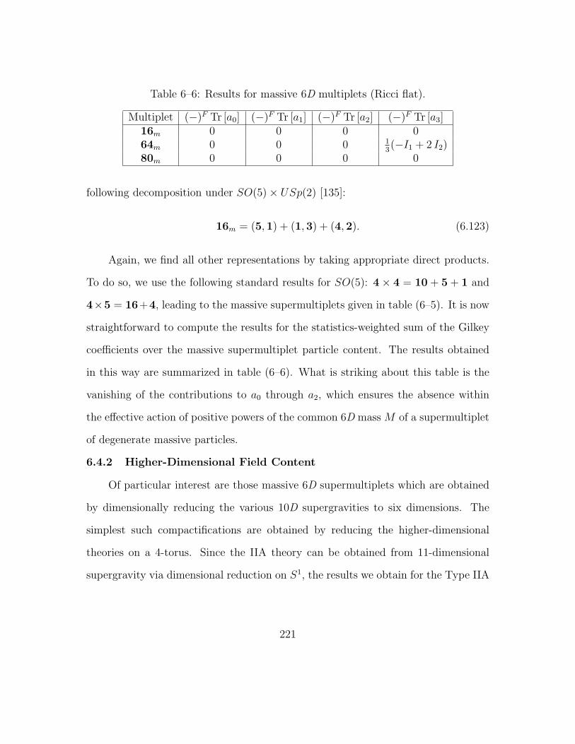
Table 6–6: Results for massive 6D multiplets (Ricci flat).

Multiplet (−)F Tr [a0] (−)F Tr [a1] (−)F Tr [a2] (−)F Tr [a3]16m 0 0 0 064m 0 0 0 1

3(−I1 + 2 I2)

80m 0 0 0 0

following decomposition under SO(5)× USp(2) [135]:

16m = (5,1) + (1,3) + (4,2). (6.123)

Again, we find all other representations by taking appropriate direct products.

To do so, we use the following standard results for SO(5): 4× 4 = 10 + 5 + 1 and

4×5 = 16+4, leading to the massive supermultiplets given in table (6–5). It is now

straightforward to compute the results for the statistics-weighted sum of the Gilkey

coefficients over the massive supermultiplet particle content. The results obtained

in this way are summarized in table (6–6). What is striking about this table is the

vanishing of the contributions to a0 through a2, which ensures the absence within

the effective action of positive powers of the common 6D mass M of a supermultiplet

of degenerate massive particles.

6.4.2 Higher-Dimensional Field Content

Of particular interest are those massive 6D supermultiplets which are obtained

by dimensionally reducing the various 10D supergravities to six dimensions. The

simplest such compactifications are obtained by reducing the higher-dimensional

theories on a 4-torus. Since the IIA theory can be obtained from 11-dimensional

supergravity via dimensional reduction on S1, the results we obtain for the Type IIA

221

theory dimensionally reduced on a 4-torus are equivalent to what is obtained from

11-dimensional supergravity dimensionally reduced on a 5-torus.

For the purposes of the present argument all that matters is the total number

of each type of massive 6D field which is produced by such a reduction. Our purpose

in this section is to show that the massive field content which is obtained by such a

dimensional reduction is the same as would be obtained by combining a small number

of the massive 16m, 64m and 80m representations of (2,0) 6D supersymmetry.11

Since we know that each of these multiplets gives a vanishing contributions to the

first 3 heat-kernel coefficients, the same must also be true of the contributions of the

massive 6D states which are obtained by dimensional reduction.

Type IIA and type IIB supergravities

The field content of Type IIA supergravity in ten dimensions consists of: a

graviton; a 3-form, 2-form, 1-form, and 0-form; two majorana-Weyl gravitini having

opposite 10D chiralities; and two majorana-Weyl dilatini having opposite 10D chi-

ralities. The IIB theory is obtainable from the IIA theory by giving all fermions the

same chirality, and by trading the 3-form and the 1-form for a self-dual 4-form, a

2-form, and a 0-form.

Since each majorana-Weyl spinor in 10D has 16 real components, reduction on a

torus (in the absence of any Scherk-Schwartz supersymmetry-breaking twists [136])

11 This need not imply that these massive states actually transform in these repre-sentations under (2,0) supersymmetry, for example due to possible presence of centralcharges and short multiplets.

222

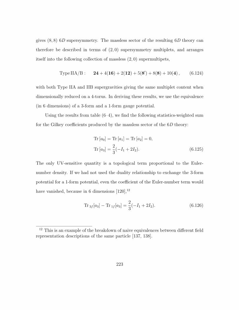
gives (8, 8) 6D supersymmetry. The massless sector of the resulting 6D theory can

therefore be described in terms of (2, 0) supersymmetry multiplets, and arranges

itself into the following collection of massless (2, 0) supermultipets,

Type IIA/B : 24 + 4(16) + 2(12) + 5(8′) + 8(8) + 10(4) , (6.124)

with both Type IIA and IIB supergravities giving the same multiplet content when

dimensionally reduced on a 4-torus. In deriving these results, we use the equivalence

(in 6 dimensions) of a 3-form and a 1-form gauge potential.

Using the results from table (6–4), we find the following statistics-weighted sum

for the Gilkey coefficients produced by the massless sector of the 6D theory:

Tr [a0] = Tr [a1] = Tr [a2] = 0,

Tr [a3] =2

3(−I1 + 2I2). (6.125)

The only UV-sensitive quantity is a topological term proportional to the Euler-

number density. If we had not used the duality relationship to exchange the 3-form

potential for a 1-form potential, even the coefficient of the Euler-number term would

have vanished, because in 6 dimensions [120],12

Tr 3f [a3]− Tr 1f [a3] =2

3(−I1 + 2I2). (6.126)

12 This is an example of the breakdown of naive equivalences between different fieldrepresentation descriptions of the same particle [137, 138].

223

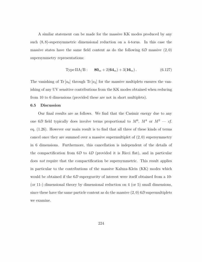
A similar statement can be made for the massive KK modes produced by any

such (8, 8)-supersymmetric dimensional reduction on a 4-torus. In this case the

massive states have the same field content as do the following 6D massive (2, 0)

supersymmetry representations:

Type IIA/B : 80m + 2(64m) + 3(16m) . (6.127)

The vanishing of Tr [a0] through Tr [a2] for the massive multiplets ensures the van-

ishing of any UV sensitive contributions from the KK modes obtained when reducing

from 10 to 6 dimensions (provided these are not in short multiplets).

6.5 Discussion

Our final results are as follows. We find that the Casimir energy due to any

one 6D field typically does involve terms proportional to M6, M4 or M2 — cf.

eq. (1.26). However our main result is to find that all three of these kinds of terms

cancel once they are summed over a massive supermultiplet of (2, 0) supersymmetry

in 6 dimensions. Furthermore, this cancellation is independent of the details of

the compactification from 6D to 4D (provided it is Ricci flat), and in particular

does not require that the compactification be supersymmetric. This result applies

in particular to the contributions of the massive Kaluza-Klein (KK) modes which

would be obtained if the 6D supergravity of interest were itself obtained from a 10-

(or 11-) dimensional theory by dimensional reduction on 4 (or 5) small dimensions,

since these have the same particle content as do the massive (2, 0) 6D supermultiplets

we examine.

224

As such, we believe these results to be encouraging for the success of the SLED

program, inasmuch as they show how bulk supersymmetry can stop very heavy KK

particles from contributing too large one-loop amounts to the low-energy effective

cosmological constant, both through bulk and brane-localized effective interactions.

These results leave one type of one-loop contribution which could still be dangerously

large from the SLED point of view: dimension-two interactions localized on the brane

(such as a brane-localized Einstein-Hilbert action) which are generated by loops of

brane-bound particles (for which supersymmetry is badly broken). Indeed, such

effective interactions are likely to be generated by brane loops, and it is not yet clear

whether the bulk response need cancel their 4D effects in the same way as it would

do for an effective brane tension.

225

CHAPTER 7Conclusions

In this thesis we examined critical aspects of Supersymmetric Large Extra Di-

mensions, a proposal whose goal is to address both the cosmological constant and the

hierarchy problems. Since the SLED proposal relies critically on 6D supergravity,

part of our investigation focused on finding new solutions to the relevant equations

of motion. When work began on this thesis, very little was known about the so-

lutions to the supergravity of interest to us, Nishino-Sezgin supergravity. Progress

in this direction was considerably improved thanks to Gibbons, Gueven and Pope

(GGP), who found the most general solution to the equations of motion, subject to

the requirements of having 4D Minkowski space and axial symmetry in the extra

dimensions. As discussed in the introductory chapter, they also showed that the

unique singularity-free solution consistent with maximal symmetry of the four large

dimensions is the one found by Salam and Sezgin, corresponding to 4D Minkowski

space and spherical extra dimensions.

One of the questions we answer in chapter 3 is what happens when we relax the

requirement that solutions be 4D-flat. In that case, we show that Minkowski space is

no longer the only maximally-symmetric solution allowed; in particular, we explicitly

find solutions having both de Sitter and anti-de Sitter symmetry which necessarily

involve non-conical singularities. This result is important since it shows that in the

226

presence of branes — which generically induce singularities at their location — 4D-

flat solutions are not guaranteed in the same way that they are in the absence of

branes. In this chapter we also find time-dependent solutions to the 6D equations

of motion. These are ‘scaling’ solutions since the time dependence factors out of all

equations of motion, which corresponds to a considerable simplification. Ultimately,

it must be determined whether the SLED proposal yields acceptable cosmologies,

and so finding time-dependent solutions is a necessary first step in this direction.

It is also important to determine whether the various solutions of the super-

gravity equations of motion are stable against small perturbations. Obviously, a

solution who timescale for decay is much less than the age of the universe does not

yield a good cosmological model. Thus, in chapter 4 we examine the perturbative

stability of a large class of solutions to Nishino-Sezgin supergravity. We do so by

linearizing the relevant equations of motion about the general time-independent so-

lutions found by GGP. We solve the resulting linearized equations of motion exactly

in the case where the background GGP solution is chosen to be conical, and then

show that for appropriate boundary conditions all modes have masses greater than

or equal to zero. For the more general case where the background is nonconical, we

can no longer write closed-form solutions; nonetheless, we show that the solutions

are marginally stable, subject again to appropriate boundary conditions. Here, the

marginal stability is expected since scale invariance ensures that there is a massless

mode. Finally, we conclude by closing a possible loophole in the above analysis by

showing that there are no ghosts present.

227

In chapter 5 we turn to the issue of how to regularize singularities in the case

where the metric is not conical in the vicinity of brane sources since, as it turns out,

the majority of singularities encountered are not conical in nature. For example,

in the case of the GGP solutions we see that the conical solutions satisfy λ1 = λ2,

and so make up only a tiny fraction of the parameter space of solutions. Thus, it

is important to understand what objects source these more exotic singularities. To

smooth out these singularities, we excise small regions of space in the neighbour-

hood of the singular points, and on the boundaries of these excised regions we place

codimension-1 branes. The interior regions are then filled with non-singular solutions

to the equations of motion. Our analysis shows in detail how these branes dictate

various bulk properties; for example, we show that there is a ‘Hamiltonian constraint’

which the branes must satisfy if there are to source a flat bulk solution. We further

identify the brane properties required to ensure unbroken scale invariance. Finally,

we calculate the low-energy effective potential for the mode corresponding to this

scaling symmetry, and as expected we find that it is zero in the case where the scale

invariance is unbroken.

The purpose of chapter 6 is to address the all-important question of the size of

the Casimir energy induced by bulk loops. In order that these results be as general as

possible, we do not restrict ourselves to working only in six dimensions and so keep

the number of dimensions arbitrary. We calculate the first few heat kernel coefficients

for the fields up to spin 2, including the contributions of the ghosts. While similar

calculations have been performed in the past for massless particles [120], our main

extension is to provide n-dimensional results for massive fields rather than massless

228

fields, as well as to extend these results to spacetimes having more general background

geometries. This includes calculating the contributions of the various ghosts and

would-be Goldstone particles which participate in the generalized higher-spin mass-

acquisition (Higgs) mechanism. We then assemble these results into supermultiplets

in order to obtain the heat kernel coefficients for general supergravity theories. It is

shown how once assembled into massive supermultiplets, these coefficients vanish in

a number of cases.

Future directions

While much progress has been made in determining the viability of the SLED

proposal, there is work that still needs to be done. In chapter 3 we present a number

of new exact solutions to the 6D supergravity equations of motion, although it is

obvious that these solutions describe only a tiny subset of possible behaviours of this

system. For example, all known solutions currently assume that the extra dimensions

are axially symmetric, and so one possible avenue of research is to search for solutions

where this assumption is relaxed. As suggested in [139], such solutions may represent

the endpoint of a decay from one of the unstable solutions of NS supergravity.

Another area for future research is in improving our understanding of brane-

induced singularities. While chapter 5 focuses on regularizing these singularities by

modeling the brane as having a finite thickness, such a procedure requires solving

complicated algebraic equations for many unknowns. It would be therefore be bene-

ficial to have a more direct handle on how the renormalization of these singularities

should proceed. For example, in the case of a fixed background geometry which

229

is conical, references [88] and [89, 90] show in detail how the various brane cou-

plings renormalize. A generalization of these results to more general backgrounds is

currently underway.

Finally, given the critical importance to the SLED proposal of determining the

size of the one-loop quantum corrections, it certainly behooves us to determine the

answer to this question in the case of the general GGP solutions. As mentioned in

chapter 6, this involves disentangling the mixings between fields of different spin,

induced by the nontrivial background geometry. Once this is accomplished, the

general results of chapter 6 can be used to determine these one-loop corrections.

Work on this is currently in progress.

230

APPENDIX ANewton’s Law in Higher Dimensions

In this appendix, we show how Newton’s law is derived from the Einstein-Hilbert

action. This justifies the claim that the usual inverse square law (ISL) of gravity is

modified to a “1/r2+d law” when there are d extra dimensions. We also show how

the ISL is recovered at low energies, for the special case where the extra dimensions

are compact. A more detailed treatment of this transition can be found in [140].

To see how Newton’s law is derived in higher-dimensional gravity, we recall that

in the Newtonian limit the only non-trivial metric component is g00 = −(1 + 2φ),

and so the only nonzero component of the Einstein tensor is G00 ≈ ∇2g00 = −2∇2φ.

Thus, using also that T00 = ρ is the energy density of nonrelativistic matter, we

obtain

∇2φ =ρ

2M2+d∗

(A.1)

and so recognize φ as the usual gravitational potential. Applying Gauss’ law we see

that for d extra dimensions the gravitational force is given by

F =G∗m1m2

r2+d, (A.2)

which defines the higher-dimensional Newton constant by G−1∗ = 2 Ω2+dM

2+d∗ , where

Ωn is the surface area of the unit n-sphere. Using this last result together with

eq. (1.17), we obtain the expression for the 4D Newton constant in terms of the

231

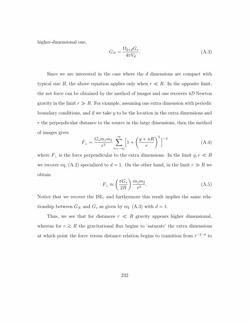
higher-dimensional one,

GN =Ω2+dG∗

4πVd. (A.3)

Since we are interested in the case where the d dimensions are compact with

typical size R, the above equation applies only when r R. In the opposite limit,

the net force can be obtained by the method of images and one recovers 4D Newton

gravity in the limit r R. For example, assuming one extra dimension with periodic

boundary conditions, and if we take y to be the location in the extra dimensions and

r the perpendicular distance to the source in the large dimensions, then the method

of images gives

F⊥ =G∗m1m2

r3

∞∑n=−∞

[1 +

(y + nR

r

)2 ]−2

(A.4)

where F⊥ is the force perpendicular to the extra dimensions. In the limit y, r R

we recover eq. (A.2) specialized to d = 1. On the other hand, in the limit r R we

obtain

F⊥ ≈(πG∗2R

)m1m2

r2. (A.5)

Notice that we recover the ISL, and furthermore this result implies the same rela-

tionship between GN and G∗ as given by eq. (A.3) with d = 1.

Thus, we see that for distances r R gravity appears higher dimensional,

whereas for r >∼ R the gravitational flux begins to ‘saturate’ the extra dimensions

at which point the force versus distance relation begins to transition from r−2−d to

232

r−2. In the SLED proposal, this dilution of gravitational flux into the extra dimen-

sions is the ultimate reason why gravity is perceived to be so much weaker than the

electroweak force even though we assume M∗ ∼MEW.

233

APPENDIX BSome Special Functions

In this appendix we record some useful properties of the special functions which

are used in the main text. In our conventions the Legendre functions are related to

Hypergeometric functions by

Pν(z) = F

[−ν, 1 + ν; 1;

1

2(1− z)

]Qν(z) =

√π Γ(1 + ν)

(2z)1+νΓ(

32

+ ν) F [1 +

ν

2,1

2+ν

2;3

2+ ν; z−2

], ν 6= −3

2,−5

2, . . . .

The asymptotic form of the Legendre functions as z → ±1 can be found from

well-established properties of the hypergeometric functions, most notably its series

definition

F [a, b; c; z] = 1 +ab

cz +

a(a+ 1)b(b+ 1)

c(c+ 1)

z2

2!+ · · · , (B.1)

provided c 6= 0,−1,−2, . . . . For |z| < 1 the hypergeometric function has the property

F [a, b; c; z] = (1− z)c−a−bF [c− a, c− b; c; z]. (B.2)

The potential singularities of F [a, b; c; z] lie at z = ±1 and z =∞, and our interest is

in particular its behaviour at z = ±1. A useful identity, valid when |arg(1− z)| < π,

234

for identifying these behaviours is

F [a, b; c;u] =Γ(c)Γ(c− a− b)Γ(c− b)Γ(c− a)

F [a, b; 1 + a+ b− c; 1− u] (B.3)

+(1− u)c−a−b[

Γ(c)Γ(a+ b− c)Γ(a)Γ(b)

]F [c− a, c− b; c− a− b+ 1; 1− u] .

This expression shows that F [a, b; c; z] is finite as z → 1 provided c > a+b, it diverges

there logarithmically if c = a+ b, and it can be more singular if c < a+ b:

F [a, b; c; 1] =Γ(c) Γ(c− a− b)Γ(c− a) Γ(c− b)

, if c > a+ b, a, b /∈ Z−

F [a, b; a+ b; z] −−→z→1

− Γ(a+ b)

Γ(a)Γ(b)log(1− z), if a, b /∈ Z−

F [−n, b; c; 1] =(c− b)n

(c)n, n ∈ N .

Here Γ is Euler’s Gamma function Γ(n) = (n−1)!, defined for complex arguments by

Γ(x) =∫∞

0du ux−1e−u. (· · · )n is the Pochhammer symbol, defined by (x)n = Γ(x+n)

Γ(x).

Using eq. (B.3) with a = −ν, b = 1 + ν, c = 1 and u = 12(1− z) leads (provided

ν 6= 0, 1, 2, . . . ) to the following asymptotic expression

Pν(z) = −ln[

12(1 + z)

]Γ(−ν)Γ(1 + ν)

F

[−ν, 1 + ν ; 1 ;

1

2(1 + z)

]+O(1)

= −ln[

12(1 + z)

]Γ(−ν)Γ(1 + ν)

+O(1) as z → −1 , (B.4)

If, on the other hand, ν = ` = 0, 1, . . . , then the hypergeometric series terminates

and P`(z) is bounded at both z = ±1. This leads in the usual way to the Legendre

polynomials, for which with P0(z) = 1 and:

P`(z) =1

2``!

(d

dz

)` (z2 − 1

)`, ` = 1, 2, . . . , (B.5)

235

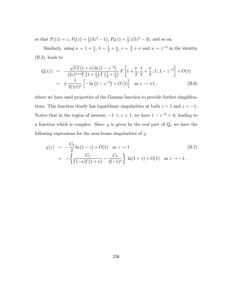
so that P1(z) = z, P2(z) = 12(3z2 − 1), P3(z) = 1

2z(5z2 − 3), and so on.

Similarly, using a = 1 + ν2, b = 1

2+ ν

2, c = 3

2+ ν and u = z−2 in the identity

(B.3), leads to

Qν(z) = −√π Γ(1 + ν) ln (1− z−2)

(2z)1+νΓ(1 + ν

2

)Γ(

12

+ ν2

) F [1 +ν

2,1

2+ν

2; 1 ; 1− z−2

]+O(1)

= ± 1

2(±1)ν

[− ln

(1− z−2

)+O (1)

]as z → ±1 , (B.6)

where we have used properties of the Gamma function to provide further simplifica-

tions. This function clearly has logarithmic singularities at both z = 1 and z = −1.

Notice that in the region of interest, −1 < z < 1, we have 1 − z−2 < 0, leading to

a function which is complex. Since χ is given by the real part of Qν we have the

following expressions for the near-brane singularities of χ:

χ(z) = −C2

2ln (1− z) +O(1) as z → 1 (B.7)

= −

C1

Γ(−ν)Γ(1 + ν)− C2

2(−1)ν

ln(1 + z) +O(1) as z → −1 .

236

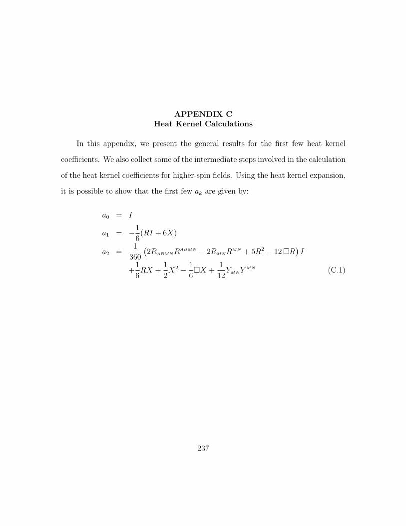
APPENDIX CHeat Kernel Calculations

In this appendix, we present the general results for the first few heat kernel

coefficients. We also collect some of the intermediate steps involved in the calculation

of the heat kernel coefficients for higher-spin fields. Using the heat kernel expansion,

it is possible to show that the first few ak are given by:

a0 = I

a1 = −1

6(RI + 6X)

a2 =1

360

(2RABMNR

ABMN − 2RMNRMN + 5R2 − 12 R

)I

+1

6RX +

1

2X2 − 1

6X +

1

12YMNY

MN (C.1)

237

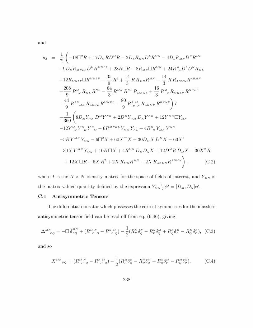
and

a3 =1

7!

(−182R + 17DMRD

MR− 2DLRMNDLRMN − 4DLRMND

NRML

+9DKRMNLPDKRMNLP + 28RR− 8RMNRMN + 24RM

NDLDNRML

+12RMNLPRMNLP − 35

9R3 +

14

3RRMNR

MN − 14

3RRABMNR

ABMN

+208

9RM

N RMLRNL − 64

3RMN RKLRMKNL +

16

3RM

N RMKLP RNKLP

−44

9RAB

MN RABKLRMNKL − 80

9RA M

B N RAKMP RBKNP

)I

+1

360

(8DMYNKD

MY NK + 2DMYNM DKYNK + 12Y MNYMN

−12Y M

N YN

K YK

M − 6RMNKL YMN YKL + 4RM

N YMK YNK

−5RY MN YMN − 62X + 60XX + 30DMX DMX − 60X3

−30X Y MN YMN + 10RX + 4RMN DMDNX + 12DMRDMX − 30X2R

+ 12X R− 5X R2 + 2X RMNRMN − 2X RABMNR

ABMN

), (C.2)

where I is the N × N identity matrix for the space of fields of interest, and YMN is

the matrix-valued quantity defined by the expression YMNij φ

j = [DM , DN ]φi.

C.1 Antisymmetric Tensors

The differential operator which possesses the correct symmetries for the massless

antisymmetric tensor field can be read off from eq. (6.46), giving

∆MN

PQ = − δMN

PQ + (RM N

P Q −RN M

P Q)− 1

2(RM

P δN

Q −RN

P δM

Q +RN

QδM

P −RM

Q δN

P ), (C.3)

and so

XMNPQ = (RM N

P Q −RN M

P Q)− 1

2(RM

P δN

Q −RN

P δM

Q +RN

QδM

P −RM

Q δN

P ). (C.4)

238

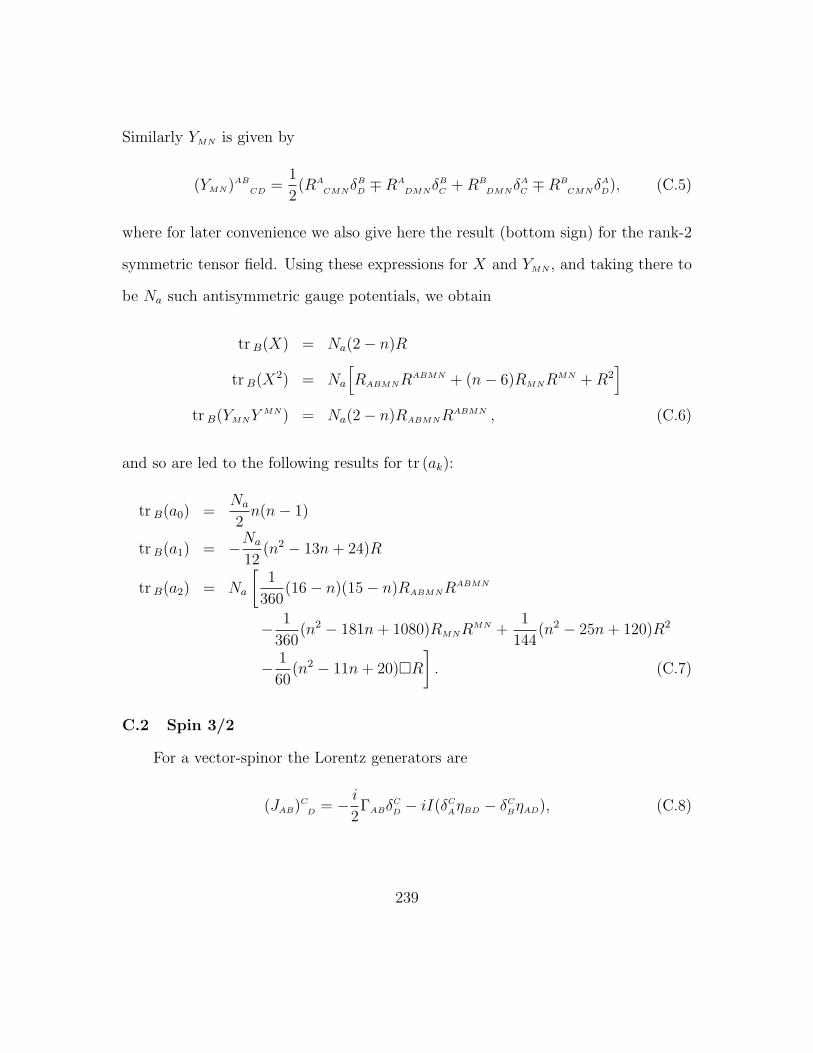
Similarly YMN is given by

(YMN)ABCD =1

2(RA

CMNδB

D ∓RA

DMNδB

C +RB

DMNδA

C ∓RB

CMNδA

D), (C.5)

where for later convenience we also give here the result (bottom sign) for the rank-2

symmetric tensor field. Using these expressions for X and YMN , and taking there to

be Na such antisymmetric gauge potentials, we obtain

tr B(X) = Na(2− n)R

tr B(X2) = Na

[RABMNR

ABMN + (n− 6)RMNRMN +R2

]tr B(YMNY

MN) = Na(2− n)RABMNRABMN , (C.6)

and so are led to the following results for tr (ak):

tr B(a0) =Na

2n(n− 1)

tr B(a1) = −Na

12(n2 − 13n+ 24)R

tr B(a2) = Na

[1

360(16− n)(15− n)RABMNR

ABMN

− 1

360(n2 − 181n+ 1080)RMNR

MN +1

144(n2 − 25n+ 120)R2

− 1

60(n2 − 11n+ 20)R

]. (C.7)

C.2 Spin 3/2

For a vector-spinor the Lorentz generators are

(JAB)CD = − i2

ΓABδC

D − iI(δCAηBD − δCBηAD), (C.8)

239

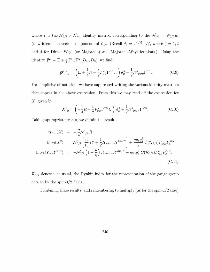
where I is the N3/2 × N3/2 identity matrix, corresponding to the N3/2 = N3/2 ds

(unwritten) non-vector components of ψM . (Recall ds = 2[n/2]+1/ζ, where ζ = 1, 2

and 4 for Dirac, Weyl (or Majorana) and Majorana-Weyl fermions.) Using the

identity /D2 = + 14[ΓM ,ΓN ][DM , DN ], we find

[ /D2]AB =

( +

1

4R− i

2F aCDΓCD ta

)δAB −

1

2RA

BCDΓCD. (C.9)

For simplicity of notation, we have suppressed writing the various identity matrices

that appear in the above expression. From this we may read off the expression for

X, given by

XA

B =

(−1

4R +

i

2F aCDΓCD ta

)δAB +

1

2RA

BMNΓMN . (C.10)

Taking appropriate traces, we obtain the results

tr V S(X) = − n4N3/2R

tr V S(X2) = N3/2

[n

16R2 +

1

2RABMNR

ABMN

]+ndsg

2a

2C(R3/2)F a

MNFMN

a

tr V S (YMNYMN) = −N3/2

(1 +

n

8

)RABMNR

ABMN − ndsg2a C(R3/2)F a

MNFMN

a .

(C.11)

R3/2 denotes, as usual, the Dynkin index for the representation of the gauge group

carried by the spin-3/2 fields.

Combining these results, and remembering to multiply (as for the spin-1/2 case)

240

eq. (C.1) by an overall factor of 1/2, we find

tr V S(a0) =n

2N3/2

tr V S(a1) =n

24N3/2R

tr V S(a2) =N3/2

360

[(30− 7n

8

)RABMNR

ABMN − nRMNRMN +

5n

8R2 +

3n

2R

]+ndsg

2a

12C(R3/2)F a

MNFMN

a . (C.12)

C.3 Spin 2

From eq. (6.89), the symmetric traceless differential operator appropriate for

φMN is seen to be

∆MN

PQ = −[ + (R + 2Λ)

]δMN

PQ + (RM N

P Q +RN M

P Q)− 4

n(gPQR

MN + gMNRPQ)

+1

2(RM

P δN

Q +RN

P δM

Q +RN

QδM

P +RM

Q δN

P ) +4

n2gMNgPQR , (C.13)

from which the expression for X can be read off directly. Taking traces of the relevant

quantities, we find

tr symtr(X) = N2

[− 1

2n(n+ 2)(n2 − 3n+ 4)R− (n+ 2)(n− 1)Λ

]tr symtr(X

2) = N2

[3RABMNR

ABMN +1

n(n2 − 2n− 32)RMNR

MN

+1

2n2(n4 − 3n3 + 16n+ 32)R2

+2

n(n+ 2)(n2 − 3n+ 4)ΛR + 2(n+ 2)(n− 1)Λ2

]tr symtr(YMNY

MN) = −N2(n+ 2)RABMNRABMN . (C.14)

241

Applying eq. (C.1), we arrive at the following expressions for tr [ak]:

tr symtr(a0) =N2

2(n+ 2)(n− 1)

tr symtr(a1) = N2

[1

12n(n+ 2)(5n2 − 17n+ 24)R + (n+ 2)(n− 1)Λ

]tr symtr(a2) = N2

[1

360(n2 − 29n+ 478)RABMNR

ABMN (C.15)

− 1

360n(n3 − 179n2 + 358n+ 5760)RMNR

MN

+1

144n2(25n4 − 95n3 + 22n2 + 480n+ 1152)R2

+1

30n(n+ 2)(2n2 − 7n+ 10)R

+1

6n(n+ 2)(5n2 − 17n+ 24)ΛR + (n2 + n− 2)Λ2

].

242

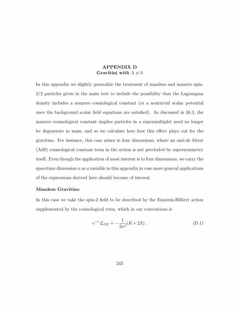
APPENDIX DGravitini with Λ 6= 0

In this appendix we slightly generalize the treatment of massless and massive spin-

3/2 particles given in the main text to include the possibility that the Lagrangian

density includes a nonzero cosmological constant (or a nontrivial scalar potential

once the background scalar field equations are satisfied). As discussed in §6.3, the

nonzero cosmological constant implies particles in a supermultiplet need no longer

be degenerate in mass, and so we calculate here how this effect plays out for the

gravitino. For instance, this case arises in four dimensions, where an anti-de Sitter

(AdS) cosmological constant term in the action is not precluded by supersymmetry

itself. Even though the application of most interest is to four dimensions, we carry the

spacetime dimension n as a variable in this appendix in case more general applications

of the expressions derived here should become of interest.

Massless Gravitino

In this case we take the spin-2 field to be described by the Einstein-Hilbert action

supplemented by the cosmological term, which in our conventions is

e−1 LEH = − 1

2κ2(R + 2Λ) . (D.1)

243

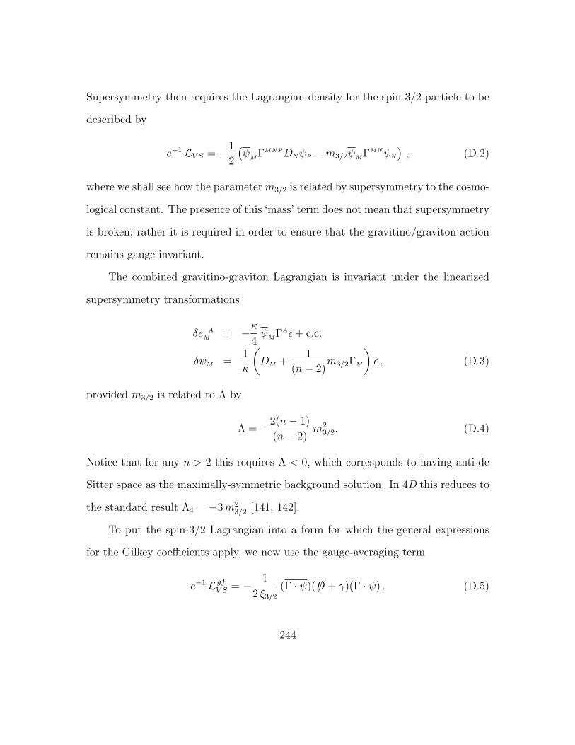
Supersymmetry then requires the Lagrangian density for the spin-3/2 particle to be

described by

e−1 LV S = −1

2

(ψMΓMNPDNψP −m3/2ψMΓMNψN

), (D.2)

where we shall see how the parameter m3/2 is related by supersymmetry to the cosmo-

logical constant. The presence of this ‘mass’ term does not mean that supersymmetry

is broken; rather it is required in order to ensure that the gravitino/graviton action

remains gauge invariant.

The combined gravitino-graviton Lagrangian is invariant under the linearized

supersymmetry transformations

δe A

M = −κ4ψMΓAε+ c.c.

δψM =1

κ

(DM +

1

(n− 2)m3/2ΓM

)ε , (D.3)

provided m3/2 is related to Λ by

Λ = −2(n− 1)

(n− 2)m2

3/2. (D.4)

Notice that for any n > 2 this requires Λ < 0, which corresponds to having anti-de

Sitter space as the maximally-symmetric background solution. In 4D this reduces to

the standard result Λ4 = −3m23/2 [141, 142].

To put the spin-3/2 Lagrangian into a form for which the general expressions

for the Gilkey coefficients apply, we now use the gauge-averaging term

e−1 L gfV S = − 1

2 ξ3/2

(Γ · ψ)( /D + γ)(Γ · ψ) . (D.5)

244

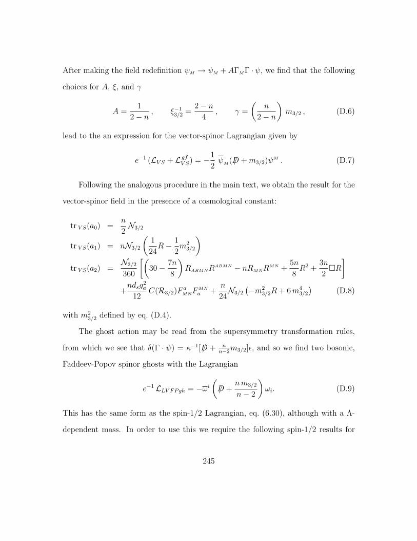
After making the field redefinition ψM → ψM +AΓMΓ · ψ, we find that the following

choices for A, ξ, and γ

A =1

2− n, ξ−1

3/2 =2− n

4, γ =

(n

2− n

)m3/2 , (D.6)

lead to the an expression for the vector-spinor Lagrangian given by

e−1 (LV S + L gfV S) = −1

2ψM( /D +m3/2)ψM . (D.7)

Following the analogous procedure in the main text, we obtain the result for the

vector-spinor field in the presence of a cosmological constant:

tr V S(a0) =n

2N3/2

tr V S(a1) = nN3/2

(1

24R− 1

2m2

3/2

)tr V S(a2) =

N3/2

360

[(30− 7n

8

)RABMNR

ABMN − nRMNRMN +

5n

8R2 +

3n

2R

]+ndsg

2a

12C(R3/2)F a

MNFMN

a +n

24N3/2

(−m2

3/2R + 6m43/2

)(D.8)

with m23/2 defined by eq. (D.4).

The ghost action may be read from the supersymmetry transformation rules,

from which we see that δ(Γ · ψ) = κ−1[ /D + nn−2

m3/2]ε, and so we find two bosonic,

Faddeev-Popov spinor ghosts with the Lagrangian

e−1 LLV FPgh = −ωi(

/D +nm3/2

n− 2

)ωi. (D.9)

This has the same form as the spin-1/2 Lagrangian, eq. (6.30), although with a Λ-

dependent mass. In order to use this we require the following spin-1/2 results for

245

the Gilkey-DeWitt coefficients quoted in the main text, generalized to include the

fermion mass, m2, inside X:

tr 1/2(a0) =N1/2

2

tr 1/2(a1) =N1/2

24(R− 12m2)

tr 1/2(a2) =N1/2

360

[−7

8RABMNR

ABMN −RMNRMN +

5

8(R− 12m2)2 +

3

2R

]+dsg

2a

12C(R1/2)F a

MNFMN

a . (D.10)

The Faddeev-Popov ghost result for tr [ak] is then obtained by multiplying these

expressions by −2, and specializing to the ‘mass’ m = nm3/2/(n− 2).

The use of the operator ( /D+ γ) in the gauge-fixing Lagrangian, eq. (D.5), leads

to a bosonic, Nielsen-Kallosh ghost. Rewriting γ in terms of m3/2, we see that the

Nielsen-Kallosh ghost has the Lagrangian

e−1 LLV NKgh = −ω(

/D −nm3/2

n− 2

)ω. (D.11)

This ghost therefore contributes −1 times the spin-1/2 result to tr [ak], with m =

−nm3/2/(n− 2).

Adding the vector-spinor result together with its associated ghosts, we obtain

the following contribution to tr [ak] by physical spin-3/2 states in the presence of a

246

cosmological constant:

tr 3/2(a0) =N3/2

2(n− 3)

tr 3/2(a1) =N3/2

24

((n− 3)R +

6n(n2 − 7n+ 4)

(n− 1)(n− 2)Λ

)tr 3/2(a2) =

N3/2

360

[(30− 7

8(n− 3)

)RABMNR

ABMN − (n− 3)RMNRMN

+5

8(n− 3)R2 +

3

2(n− 3)R +

15n(n2 − 7n+ 4)ΛR

2(n− 1)(n− 2)

+45n(n4 − 11n3 + 24n2 − 32n+ 16)Λ2

2(n− 1)2(n− 2)2

]+dsg

2a

12(n− 3)C(R3/2)F a

MNFMN

a . (D.12)

Massive Gravitino

This section follows closely the procedure outlined in the massive spin-3/2 section of

the main text. Starting from eq. (6.71), which was our ansatz for a massive spin-3/2

Lagrangian, we again find that this Lagrangian can be made invariant under the

supersymmetry transformations

δψM =1

κDMε+ µΓMε and δχ = fε . (D.13)

In this case, however, f is given by

f 2 = (n− 1)(n− 2)µ2 +Λ

2κ2, (D.14)

while all other equations in eq. (6.73) remain unchanged. The dependence of f on

Λ is required in order to cancel the variation of the Λ term in the Einstein-Hilbert

action.

247

Again, following the procedure of the main text, we add a gauge-fixing term,

eq. (6.76), and perform a field redefinition, eq. (6.79), in order to put the Lagrangian

into the form

e−1 (LmV S + L gfmV S) = −ψ′M( /D +m′3/2)ψ′M − χ′( /D +m′1/2)χ′. (D.15)

The parameters in the gauge-fixing Lagrangian and in the field redefinitions can be

written in terms of M and M , defined as

M = (n− 2)κµ and M =

√M2 − 2Λ

n− 2. (D.16)

With these definitions, we find

A =√

1 + β 2, B = −β2

√n− 2, C = −1

2, D = 0,

α = −1

2

√(n− 2)(1 + β 2), β =

[1

2

(n

n− 2

)M

M− 1

2

]1/2

,

m′1/2 = −γ = M, m′3/2 = M. (D.17)

For the case Λ = 0, these expressions reduce to those given in eq. (6.80). There is a

possible subtlety in the above solution, which comes about because of our simplifying

assumption to take all free parameters to be real. We see that for certain choices of

M and Λ, it’s possible that some of the parameters will be imaginary. However, in

the situations for which our results apply we expect that M |Λ|, and so in these

cases this problem will not arise.

From the gauge-fixing condition, we see that there are two Faddeev-Popov

ghosts, each with mass M , and one Nielsen-Kallosh ghost, with mass −M . The

248

one loop effective action for the ghosts is thus given by

iΣ1/2 =1

4Tr log

(M2 − /D2

)=

1

4Tr log

(M2 − 2Λ

n− 2− /D2

). (D.18)

As usual, we factor the M2 dependence out of our definition of X, and so obtain

X = −1

4R +

i

2ΓABF a

ABta −2Λ

n− 2. (D.19)

The contribution to the Gilkey coefficients coming from the three ghosts is thus

obtained by multiplying eq. (D.10) by −3, with m2 = −2Λ/(n − 2). Similarly,

the Goldstone fermion contribution is also given by eq. (D.10), again with m2 =

−2Λ/(n−2). The contribution from the vector spinor is unchanged from the massless

case considered in the main text, and so its Gilkey coefficients are given by eq. (C.12).

Summing these results, we arrive at the expression for a massive gravitino in a

background spacetime having nonzero cosmological constant:

trm3/2(a0) =N3/2

2(n− 2)

trm3/2(a1) =N3/2

24

((n− 2)R− 48Λ

n− 2

)trm3/2(a2) =

N3/2

360

[(30− 7

8(n− 2)

)RABMNR

ABMN − (n− 2)RMNRMN

+5

8(n− 2)R2 +

3

2(n− 2)R− 60ΛR

(n− 2)− 720Λ2

(n− 2)2

]+g2a

12(n− 2)dsC(R3/2)F a

MNFMN

a . (D.20)

249

REFERENCES

[1] Andrew J. Tolley, C. P. Burgess, D. Hoover, and Y. Aghababaie. Bulk singu-larities and the effective cosmological constant for higher co-dimension branes.JHEP, 03:091, 2006.

[2] A. J. Tolley, C. P. Burgess, C. de Rham, and D. Hoover. Scaling solutions to6D gauged chiral supergravity. New J. Phys., 8:324, 2006.

[3] C. P. Burgess, C. de Rham, D. Hoover, D. Mason, and A. J. Tolley. Kicking therugby ball: Perturbations of 6D gauged chiral supergravity. JCAP, 0702:009,2007.

[4] C. P. Burgess, D. Hoover, and G. Tasinato. UV Caps and Modulus Stabilizationfor 6D Gauged Chiral Supergravity. JHEP, 09:124, 2007.

[5] D. Hoover and C. P. Burgess. Ultraviolet Sensitivity in Higher Dimensions.JHEP, 01:058, 2006.

[6] C. P. Burgess and D. Hoover. UV sensitivity in supersymmetric large extradimensions: The Ricci-flat case. Nucl. Phys., B772:175–204, 2007.

[7] S. Weinberg. Gravitation and Cosmology. Wiley, New York, 1972.

[8] C. W. Misner, K. S. Thorne, and J. A. Wheeler. Gravitation. San Francisco1973, 1279p.

[9] Y. Aghababaie, C. P. Burgess, S. L. Parameswaran, and F. Quevedo. Towardsa naturally small cosmological constant from branes in 6D supergravity. Nucl.Phys., B680:389–414, 2004.

[10] W. M. Yao et al. Review of particle physics. J. Phys., G33:1–1232, 2006.

[11] P. J. Mohr and B. N. Taylor. CODATA recommended values of the fundamentalphysical constants: 1998. Rev. Mod. Phys., 72:351–495, 2000.

250

251

[12] Clifford M. Will. The confrontation between general relativity and experiment.Living Rev. Rel., 9:3, 2005.

[13] R. A. Hulse and J. H. Taylor. Discovery of a pulsar in a binary system. As-trophys. J., 195:L51–L53, 1975.

[14] C. P. Burgess. Introduction to effective field theory. Ann. Rev. Nucl. Part.Sci., 57:329–362, 2007.

[15] Joseph Polchinski. Renormalization and Effective Lagrangians. Nucl. Phys.,B231:269–295, 1984.

[16] Gerard ’t Hooft. A Property of Electric and Magnetic Flux in NonabelianGauge Theories. Nucl. Phys., B153:141, 1979.

[17] Steven Weinberg. Implications of Dynamical Symmetry Breaking: An Adden-dum. Phys. Rev., D19:1277–1280, 1979.

[18] Leonard Susskind. Dynamics of Spontaneous Symmetry Breaking in theWeinberg- Salam Theory. Phys. Rev., D20:2619–2625, 1979.

[19] Stephen P. Martin. A supersymmetry primer. 1997.

[20] George F. Smoot et al. Structure in the COBE differential microwave radiome-ter first year maps. Astrophys. J., 396:L1–L5, 1992.

[21] E. E. Falco, C. S. Kochanek, and J. A. Munoz. Limits on Cosmological ModelsFrom Radio-Selected Gravitational Lenses. Astrophys. J., 494:47–59, 1998.

[22] Adam G. Riess et al. Observational Evidence from Supernovae for an Ac-celerating Universe and a Cosmological Constant. Astron. J., 116:1009–1038,1998.

[23] S. Perlmutter et al. Measurements of Omega and Lambda from 42 High-Redshift Supernovae. Astrophys. J., 517:565–586, 1999.

[24] Brian P. Schmidt et al. The High-Z Supernova Search: Measuring CosmicDeceleration and Global Cur vature of the Universe Using Type Ia Supernovae.Astrophys. J., 507:46–63, 1998.

[25] C. P. Burgess. Supersymmetric large extra dimensions and the cosmologicalconstant problem. 2005.

252

[26] Nima Arkani-Hamed and Savas Dimopoulos. Supersymmetric unification with-out low energy supersymmetry and signatures for fine-tuning at the LHC.JHEP, 06:073, 2005.

[27] Raphael Bousso and Joseph Polchinski. Quantization of four-form fluxes anddynamical neutralization of the cosmological constant. JHEP, 06:006, 2000.

[28] Steven Weinberg. Anthropic Bound on the Cosmological Constant. Phys. Rev.Lett., 59:2607, 1987.

[29] Raman Sundrum. Towards an effective particle-string resolution of the cosmo-logical constant problem. JHEP, 07:001, 1999.

[30] Theodor Kaluza. On the Problem of Unity in Physics. Sitzungsber. Preuss.Akad. Wiss. Berlin (Math. Phys. ), 1921:966–972, 1921.

[31] O. Klein. Quantum theory and five-dimensional theory of relativity. Z. Phys.,37:895–906, 1926.

[32] Joseph Polchinski. Lectures on D-branes. 1996.

[33] M. Cvetic, G. W. Gibbons, and C. N. Pope. A string and M-theory origin forthe Salam-Sezgin model. Nucl. Phys., B677:164–180, 2004.

[34] Nima Arkani-Hamed, Savas Dimopoulos, and G. R. Dvali. The hierarchy prob-lem and new dimensions at a millimeter. Phys. Lett., B429:263–272, 1998.

[35] Nima Arkani-Hamed, Savas Dimopoulos, and G. R. Dvali. Phenomenology,astrophysics and cosmology of theories with sub-millimeter dimensions andTeV scale quantum gravity. Phys. Rev., D59:086004, 1999.

[36] Y. Aghababaie et al. Warped brane worlds in six dimensional supergravity.JHEP, 09:037, 2003.

[37] Eugene A. Mirabelli, Maxim Perelstein, and Michael Edward Peskin. Collidersignatures of new large space dimensions. Phys. Rev. Lett., 82:2236–2239, 1999.

[38] JoAnne L. Hewett and Maria Spiropulu. Particle physics probes of extra space-time dimensions. Ann. Rev. Nucl. Part. Sci., 52:397–424, 2002.

[39] Gian F. Giudice, Riccardo Rattazzi, and James D. Wells. Quantum gravityand extra dimensions at high-energy colliders. Nucl. Phys., B544:3–38, 1999.

253

[40] E. G. Adelberger, B. R. Heckel, and A. E. Nelson. Tests of the gravitationalinverse-square law. Ann. Rev. Nucl. Part. Sci., 53:77–121, 2003.

[41] C. P. Burgess, J. Matias, and F. Quevedo. MSLED: A minimal supersymmetriclarge extra dimensions scenario. Nucl. Phys., B706:71–99, 2005.

[42] Christoph Hanhart, Daniel R. Phillips, Sanjay Reddy, and Martin J. Savage.Extra dimensions, SN1987a, and nucleon nucleon scattering data. Nucl. Phys.,B595:335–359, 2001.

[43] Christoph Hanhart, Jose A. Pons, Daniel R. Phillips, and Sanjay Reddy. Thelikelihood of GODs’ existence: Improving the SN 1987a constraint on the sizeof large compact dimensions. Phys. Lett., B509:1–9, 2001.

[44] H. Nishino and E. Sezgin. Matter and Gauge Couplings of N=2 Supergravityin Six- Dimensions. Phys. Lett., B144:187, 1984.

[45] S. Randjbar-Daemi, Abdus Salam, E. Sezgin, and J. A. Strathdee. An AnomalyFree Model in Six-Dimensions. Phys. Lett., B151:351–356, 1985.

[46] Spyros D. Avramis, Alex Kehagias, and S. Randjbar-Daemi. A new anomaly-free gauged supergravity in six dimensions. JHEP, 05:057, 2005.

[47] Spyros D. Avramis and Alex Kehagias. A systematic search for anomaly-freesupergravities in six dimensions. JHEP, 10:052, 2005.

[48] Ryo Suzuki and Yuji Tachikawa. More anomaly-free models of six-dimensionalgauged supergravity. J. Math. Phys., 47:062302, 2006.

[49] Michael B. Green and John H. Schwarz. Anomaly Cancellation in Supersym-metric D=10 Gauge Theory and Superstring Theory. Phys. Lett., B149:117–122, 1984.

[50] Abdus Salam and E. Sezgin. Chiral Compactification on Minkowski x S**2 ofN=2 Einstein-Maxwell Supergravity in Six-Dimensions. Phys. Lett., B147:47,1984.

[51] Y. Aghababaie et al. Warped brane worlds in six dimensional supergravity.JHEP, 09:037, 2003.

[52] G. W. Gibbons, Rahmi Gueven, and C. N. Pope. 3-branes and uniqueness ofthe Salam-Sezgin vacuum. Phys. Lett., B595:498–504, 2004.

254

[53] C. P. Burgess, F. Quevedo, G. Tasinato, and I. Zavala. General axisymmetricsolutions and self-tuning in 6D chiral gauged supergravity. JHEP, 11:069, 2004.

[54] S. L. Parameswaran, S. Randjbar-Daemi, and A. Salvio. Gauge fields, fermionsand mass gaps in 6D brane worlds. Nucl. Phys., B767:54–81, 2007.

[55] S. L. Parameswaran, G. Tasinato, and I. Zavala. The 6D SuperSwirl. Nucl.Phys., B737:49–72, 2006.

[56] Edward Witten. Dimensional Reduction of Superstring Models. Phys. Lett.,B155:151, 1985.

[57] S. Randjbar-Daemi, Abdus Salam, and J. A. Strathdee. Spontaneous Compact-ification in Six-Dimensional Einstein- Maxwell Theory. Nucl. Phys., B214:491–512, 1983.

[58] Y. Aghababaie, C. P. Burgess, S. L. Parameswaran, and F. Quevedo. SUSYbreaking and moduli stabilization from fluxes in gauged 6D supergravity.JHEP, 03:032, 2003.

[59] (Ed. ) Salam, A. and (Ed. ) Sezgin, E. Supergravities in diverse dimensions.Vol. 1, 2. Amsterdam, Netherlands: North-Holland (1989) 1499 p. Singapore,Singapore: World Scientific (1989) 1499 p.

[60] E. Kasner. Solutions of the Einstein equations involving functions of only onevariable. Trans. Am. Math. Soc., 27:155–162, 1925.

[61] E. M. Lifshitz and I. M. Khalatnikov. Investigations in relativistic cosmology.Adv. Phys., 12:185–249, 1963.

[62] V. A. Belinsky, I. M. Khalatnikov, and E. M. Lifshitz. Oscillatory approach toa singular point in the relativistic cosmology. Adv. Phys., 19:525–573, 1970.

[63] Peter G. O. Freund and Mark A. Rubin. Dynamics of Dimensional Reduction.Phys. Lett., B97:233–235, 1980.

[64] S. Randjbar-Daemi and E. Sezgin. Scalar potential and dyonic strings in 6dgauged supergravity. Nucl. Phys., B692:346–362, 2004.

[65] Alex Kehagias. A conical tear drop as a vacuum-energy drain for the solutionof the cosmological constant problem. Phys. Lett., B600:133–141, 2004.

255

[66] S. Randjbar-Daemi and V. A. Rubakov. 4d-flat compactifications with branevorticities. JHEP, 10:054, 2004.

[67] Hyun Min Lee and Antonios Papazoglou. Brane solutions of a spherical sigmamodel in six dimensions. Nucl. Phys., B705:152–166, 2005.

[68] V. P. Nair and S. Randjbar-Daemi. Nonsingular 4d-flat branes in six-dimensional supergravities. JHEP, 03:049, 2005.

[69] Hyun Min Lee and Christoph Ludeling. The general warped solution withconical branes in six- dimensional supergravity. JHEP, 01:062, 2006.

[70] Shinji Mukohyama, Yuuiti Sendouda, Hiroyuki Yoshiguchi, and Shunichiro Ki-noshita. Warped flux compactification and brane gravity. JCAP, 0507:013,2005.

[71] Ignacio Navarro and Jose Santiago. Gravity on codimension 2 brane worlds.JHEP, 02:007, 2005.

[72] Bryce S. DeWitt. The global approach to quantum field theory. Vol. 1, 2. Int.Ser. Monogr. Phys., 114:1–1042, 2003.

[73] Andreas Albrecht, C. P. Burgess, F. Ravndal, and C. Skordis. Naturalquintessence and large extra dimensions. Phys. Rev., D65:123507, 2002.

[74] Andrew J. Tolley, C. P. Burgess, Claudia de Rham, and D. Hoover. ExactWave Solutions to 6D Gauged Chiral Supergravity. 2007.

[75] Hyun Min Lee and Antonios Papazoglou. Scalar mode analysis of the warpedSalam-Sezgin model. Nucl. Phys., B747:294–311, 2006.

[76] James M. Cline, Julie Descheneau, Massimo Giovannini, and Jeremie Vinet.Cosmology of codimension-two braneworlds. JHEP, 06:048, 2003.

[77] Lisa Randall and Raman Sundrum. A large mass hierarchy from a small extradimension. Phys. Rev. Lett., 83:3370–3373, 1999.

[78] Lisa Randall and Raman Sundrum. An alternative to compactification. Phys.Rev. Lett., 83:4690–4693, 1999.

[79] Robert Geroch and Jennie H. Traschen. Strings and Other DistributionalSources in General Relativity. Phys. Rev., D36:1017, 1987.

256

[80] Jeremie Vinet and James M. Cline. Can codimension-two branes solve thecosmological constant problem? Phys. Rev., D70:083514, 2004.

[81] Marco Peloso, Lorenzo Sorbo, and Gianmassimo Tasinato. Standard 4d gravityon a brane in six dimensional flux compactifications. Phys. Rev., D73:104025,2006.

[82] Eleftherios Papantonopoulos, Antonios Papazoglou, and Vassilios Zamarias.Regularization of conical singularities in warped six- dimensional compactifi-cations. JHEP, 03:002, 2007.

[83] Marco Peloso, Lorenzo Sorbo, and Gianmassimo Tasinato. Standard 4d gravityon a brane in six dimensional flux compactifications. Phys. Rev., D73:104025,2006.

[84] Tsutomu Kobayashi and Masato Minamitsuji. Gravity on an extended brane insix-dimensional warped flux compactifications. Phys. Rev., D75:104013, 2007.

[85] Burak Himmetoglu and Marco Peloso. Isolated Minkowski vacua, and stabilityanalysis for an extended brane in the rugby ball. Nucl. Phys., B773:84–104,2007.

[86] Paul Bostock, Ruth Gregory, Ignacio Navarro, and Jose Santiago. Einsteingravity on the codimension 2 brane? Phys. Rev. Lett., 92:221601, 2004.

[87] Olindo Corradini, Alberto Iglesias, Zurab Kakushadze, and Peter Langfelder.Gravity on a 3-brane in 6D bulk. Phys. Lett., B521:96–104, 2001.

[88] Walter D. Goldberger and Mark B. Wise. Renormalization group flows forbrane couplings. Phys. Rev., D65:025011, 2002.

[89] Claudia de Rham. The Effective Field Theory of Codimension-two Branes.JHEP, 01:060, 2008.

[90] Claudia de Rham. Classical Renormalization of Codimension-two Brane Cou-plings. AIP Conf. Proc., 957:309–312, 2007.

[91] Walter D. Goldberger and Mark B. Wise. Modulus stabilization with bulkfields. Phys. Rev. Lett., 83:4922–4925, 1999.

[92] G. W. Gibbons and S. W. Hawking. Action Integrals and Partition Functionsin Quantum Gravity. Phys. Rev., D15:2752–2756, 1977.

257

[93] G. W. Gibbons and C. N. Pope. Consistent S**2 Pauli reduction ofsix-dimensional chiral gauged Einstein-Maxwell supergravity. Nucl. Phys.,B697:225–242, 2004.

[94] W. Israel. Singular hypersurfaces and thin shells in general relativity. NuovoCim., B44S10:1, 1966.

[95] Jan de Boer, Erik P. Verlinde, and Herman L. Verlinde. On the holographicrenormalization group. JHEP, 08:003, 2000.

[96] Peter B. Gilkey. The Spectral geometry of a Riemannian manifold. J. Diff.Geom., 10:601–618, 1975.

[97] S. M. Christensen. Regularization, Renormalization, and Covariant GeodesicPoint Separation. Phys. Rev., D17:946–963, 1978.

[98] S. M. Christensen and M. J. Duff. New Gravitational Index Theorems andSupertheorems. Nucl. Phys., B154:301, 1979.

[99] D. V. Vassilevich. Heat kernel expansion: User’s manual. Phys. Rept., 388:279–360, 2003.

[100] C. P. Burgess. An ode to effective Lagrangians. 1998.

[101] C. P. Burgess. Goldstone and pseudo-Goldstone bosons in nuclear, particleand condensed-matter physics. Phys. Rept., 330:193–261, 2000.

[102] Satoshi Matsuda and Shigenori Seki. Cosmological constant probing shapemoduli through large extra dimensions. Int. J. Mod. Phys., A21:3095–3110,2006.

[103] D. M. Ghilencea, D. Hoover, C. P. Burgess, and F. Quevedo. Casimir energiesfor 6D supergravities compactified on T(2)/Z(N) with Wilson lines. JHEP,09:050, 2005.

[104] Masato Ito. Casimir forces due to matters in compactified six dimensions.Nucl. Phys., B668:322–334, 2003.

[105] Eduardo Ponton and Erich Poppitz. Casimir energy and radius stabilizationin five and six dimensional orbifolds. JHEP, 06:019, 2001.

[106] G.H. Hardy. Divergent Series. Oxford University Press, 1949.

258

[107] S. W. Hawking. Zeta Function Regularization of Path Integrals in CurvedSpace-Time. Commun. Math. Phys., 55:133, 1977.

[108] N. D. Birrell and P. C. W. Davies. Quantum fields in curved space. Cambridge,Uk: Univ. Pr. ( 1982) 340p.

[109] I.M.Ryzhik I.S. Gradshteyn. Table of Integrals, Series and Products. AcademicPress Inc., New York/London, 1965.

[110] Ruth Gregory and Caroline Santos. Cosmic strings in dilaton gravity. Phys.Rev., D56:1194–1203, 1997.

[111] J. S. Dowker. Casimir effect around a cone. Phys. Rev., D36:3095, 1987.

[112] Dmitri V. Fursaev and Sergey N. Solodukhin. On the description of the Rie-mannian geometry in the presence of conical defects. Phys. Rev., D52:2133–2143, 1995.

[113] Lara De Nardo, Dmitri V. Fursaev, and Gennaro Miele. Heat-kernel coeffi-cients and spectra of the vector Laplacians on spherical domains with conicalsingularities. Class. Quant. Grav., 14:1059–1078, 1997.

[114] Dmitri V. Fursaev and Gennaro Miele. Cones, Spins and Heat Kernels. Nucl.Phys., B484:697–723, 1997.

[115] J. A. Strathdee. Extended Poincare supersymmetry. Int. J. Mod. Phys.,A2:273, 1987.

[116] John M. Cornwall, David N. Levin, and George Tiktopoulos. Derivation ofGauge Invariance from High-Energy Unitarity Bounds on the s Matrix. Phys.Rev., D10:1145, 1974.

[117] Benjamin W. Lee, C. Quigg, and H. B. Thacker. Weak Interactions at VeryHigh-Energies: The Role of the Higgs Boson Mass. Phys. Rev., D16:1519, 1977.

[118] K. Fujikawa, B. W. Lee, and A. I. Sanda. Generalized Renormalizable GaugeFormulation of Spontaneously Broken Gauge Theories. Phys. Rev., D6:2923–2943, 1972.

[119] E. S. Abers and B. W. Lee. Gauge Theories. Phys. Rept., 9:1–141, 1973.

259

[120] E. s. Fradkin and A. a. Tseytlin. Quantization and dimensional reduction:One loop results for superyang-mills and supergravities in D>=4. Phys. Lett.,B123:231–236, 1983.

[121] E. S. Fradkin and A. A. Tseytlin. Conformal Anomaly in Weyl Theory andAnomaly Free Superconformal Theories. Phys. Lett., B134:187, 1984.

[122] W. Siegel. Hidden Ghosts. Phys. Lett., B93:170, 1980.

[123] Soo-Jong Rey. The Higgs mechanism for Kalb-Ramond gauge field. Phys. Rev.,D40:3396, 1989.

[124] N. K. Nielsen. Ghost counting in supergravity. Nucl. Phys., B140:499, 1978.

[125] R. E. Kallosh. Modified Feynman Rules in Supergravity. Nucl. Phys.,B141:141–152, 1978.

[126] C. P. Burgess, E. Filotas, M. Klein, and F. Quevedo. Low-energy brane-worldeffective actions and partial supersymmetry breaking. JHEP, 10:041, 2003.

[127] S. Ferrara and P. van Nieuwenhuizen. Noether coupling of massive gravitinosto N=1 supergravity. Phys. Lett., B127:70, 1983.

[128] Richard Altendorfer and Jonathan Bagger. Dual supersymmetry algebras frompartial supersymmetry breaking. Phys. Lett., B460:127–134, 1999.

[129] S. M. Christensen and M. J. Duff. Quantizing Gravity with a CosmologicalConstant. Nucl. Phys., B170:480, 1980.

[130] Y. M. Cho and S. W. Zoh. Explicit construction of massive spin two fields inKaluza-Klein theory. Phys. Rev., D46:2290–2294, 1992.

[131] Z. Chacko, M. Graesser, C. Grojean, and L. Pilo. Massive gravity on a brane.Phys. Rev., D70:084028, 2004.

[132] M. Fierz and W. Pauli. On relativistic wave equations for particles of arbitraryspin in an electromagnetic field. Proc. Roy. Soc. Lond., A173:211–232, 1939.

[133] Yu. M. Zinoviev. Massive spin-2 supermultiplets. 2002.

[134] S. Deser and Rafael I. Nepomechie. Gauge invariance versus masslessness inde Sitter space. Ann. Phys., 154:396, 1984.

260

[135] J. A. Strathdee. Extended Poincare supersymmetry. Int. J. Mod. Phys.,A2:273, 1987.

[136] Joel Scherk and John H. Schwarz. Spontaneous Breaking of SupersymmetryThrough Dimensional Reduction. Phys. Lett., B82:60, 1979.

[137] S. M. Christensen, M. J. Duff, G. W. Gibbons, and M. Rocek. Vanishing oneloop beta function in gauged N > 4 supergravity. Phys. Rev. Lett., 45:161,1980.

[138] M. J. Duff and P. van Nieuwenhuizen. Quantum Inequivalence of DifferentField Representations. Phys. Lett., B94:179, 1980.

[139] S. L. Parameswaran, S. Randjbar-Daemi, and A. Salvio. Stability and NegativeTensions in 6D Brane Worlds. JHEP, 01:051, 2008.

[140] P. Callin and C. P. Burgess. Deviations from Newton’s law in supersymmetriclarge extra dimensions. Nucl. Phys., B752:60–79, 2006.

[141] P. K. Townsend. Cosmological Constant in Supergravity. Phys. Rev.,D15:2802–2804, 1977.

[142] B. de Wit. Introduction to supergravity. Lectures given at 1984 Spring Schoolon Supersymmetry and Supergravity, Trieste, Italy, Apr 4-14, 1984.