SUPERPOSITION IN THE INTERPRETATION OF TWO … · To determine the resistivity index when this line does not lie over the observation sheet, the secondary 'indices are drawn on the

If you do not need this publication after it has served your purpose, please return it to the Geological Survey, using the official mailing label at the end

UNITED STATES DEPARTMENT OF THE INTERIOR

SUPERPOSITION IN THEINTERPRETATION OF TWO-LAYER

EARTH-RESISTIVITY CURVES

GEOLOGICAL SURVEY BULLETIN 927-A

UNITED STATES DEPARTMENT OF THE INTERIOR Harold L. Ickes, Secretary

GEOLOGICAL SURVEY W. C. Mendenhall, Director

Bulletin 927-A

SUPERPOSITION IN THE INTERPRETATION OF TWO-LAYER EARTH-RESISTIVITY CURVES

BY

IRWIN ROMAN

Contributions to geophysics 1941

(Pages 1-18)

UNITED STATES

GOVERNMENT PRINTING OFFICE

WASHINGTON : 1941

'IK Fale by the Superintendent of Documents, Washington, D. C. ....... Price 30 cent*

CONTENTS

PageAbstract. _____________--___-_-____--___-_______-___---_______----- 1Introduction.__-_____--_-__-_-___-_-_-_-_---_---_---_-_______-_--_ 1Theoretical principles______________________________________________ 3Explanation of the tables and graphs ___-___---__--____--_______-____ 4Preparation of the reference charts __________________________________ 6The superposition method of interpretation._--__-____.-_._________-__ 10An illustrative example__-___________-___---_-_-_-___-__-____----- 12Discussion._______________________________________________________ 14

Applicability of the partition method.__---_-___-__--_______-____ 15Modification of the measuring system.__--____-_-___-_.________-_ 15Reliability___.___________;_________.______________.-.._ 15Homogeneity and isotropism.___________________________________ 15Average resistivity....________-___._-_---_-___-----___-_-_-__-_ 15Partial superposition.__________________________________________ 16Uniqueness. _-____--________.________-_-_---_-_---_--.__---__- 17

ILLUSTKATIONS

Page PLATE 1. Reference chart for buried insulators___________________ In pocket

2. Reference chart for buried conductors._________________ In pocketFIGURE 1. Assumed geologic conditions and basic measuring systems for

use in the interpretation of two-layer earth-resistivity curves _ 2 2. Superposition graph for illustrative example ________________ 13

TABLES

Page TABLE 1. Bed-correction values____________.________________________ 6

2. Reference-chart coordinates for buried insulator. __________ ___ 83. Reference-chart coordinates for buried conductor.____________ 94. Plotting table...______________________^_-________^_^___ In pocket5. Interpretation table._______________^_^________________ In pocket6. Data for illustrative example.______________________ 137. Values of V for reference curve in p6sition shown in figure 2_ _ _ _ 14

n

OONTBIBUTIONS-TO GEOPHYSICS, 1941

SUPERPOSITION IN THE INTERPRETATION OF TWO- LAYER EARTH-RESISTIVITY CURVES

By IRWIN ROMAN

A method is presented for the interpretation of data on electrical resistivity by the superposition of standard reference curves on those obtained from field observations. This method is applicable where bedrock whose average resistivity is essentially uniform is overlain by overburden whose average resistivity is also uniform but markedly distinct.

Instructions for using this method are so given that the routine work may be done by persons not trained in geophysics or advanced mathematics. These in structions are followed by a discussion of the applicability of the method, whose reliability is affected by many factors. Bedrock and overburden, for example, may each comprise many different layers that do not materially affect the homogeneity and isotropism of the formations as a whole; on the other hand, individual layers may affect so large a part of the resistivity curve that the method cannot.be ap plied. In spite of such conditions, however, partial superposition may give valuable qualitative results. If the resistivity curve is unique, the superposition method should give essentially exact results; if several curves are very similar, or if a curve has a very slight degree of curvature, the results of superposition will be correspondingly indefinite.

INTRODUCTION 1

In two previous papers 1 a- method was described for interpreting simple resistivity curves by superposing the observed curves on a set of reference curves. The principles were discussed, and the reference curves were shown on reduced scales. As these two papers contain numerous references to prior literature, no bibliography has been in cluded in the present paper, beyond reference to a few papers bearing on specific items of the text. The reader may find bibliographies in several places, if he is interested in the historical aspects of the subject.

The purpose of the present paper is to summarize the preceding papers and to reduce them to a form available immediately to the user.

' Roman, Irwin, How to compute tables for determining electrical resistivity of underlying beds and their application to geophysical problems: U. S. Bur. Mines Tech. Paper 502, especially p. 22,1931; Some inter pretations of earth-resistivity data: Am. Inst. Min. Met. Eng., Geophysical prospecting, 1934, pp. 183-197.

1

2 CONTRIBUTIONS TO GEOPHYSICS, 1941

Although the results are given in sufficient detail to show the under lying principles, specific instructions are given that will make an ap preciation of the theory unnecessary. For this 'portion of the paper, the only requirement will be the ability to graph observations and ta use a numerical table not involving interpolation.

The assumed geologic conditions and the basic measuring configura tion are shown in figure 1. The top of the earth is considered as a plane layer of uniform thickness, h, and resistivity p 0 . This layer i& called the "overburden, "without reference to its geologic identification. Similarly, the rest of the earth is called the "bed" and is assumed to extend infinitely down and horizontally. Its resistivity, p b , is assumed

FIGURE l. Assumed geologic conditions and basic measuring system for use in the interpretation of two- layer earth-resistivity curves.

to be constant. A current, from the source S, of measured value, /,. as indicated by the meter, M, is introcluced into the ground at two points, A and B. This produces a measurable difference in potential, V, between two points, C and D, For any configuration of measuring; electrodes, an "apparent resistivity," /> , is associated with each "depth" and determined by the relation ,

pa=kV/I

in which the value of k depends on the units and on the system* of making the observations. This formula merely states that the electrical resistance is independent of the impressed current or voltage, or that Ohm's Law is valid. ...'. .

The most common system of measurement is the Wenner system, in which the points A, C, D, B are located along a straight line in the-

INTERPRETATION OF EARTH-RESISTIVITY CURVES 3

order named, each separated from its nearest neighbors by the distance a, called the "separation." In this system, the apparent resistivity is calculated from the customary relation

pa 2ir<i-T!

which assumes that the earth is a semi-infinite conductor, both homogenous and isotropic, with the surface an infinite plane.

THEORETICAL PRINCIPLES »

It has been shown 3 that the ratio of the apparent resistivity, pa , to the overburden resistivity, p 0 , may be considered as a "disturbing factor," M, whose value depends on the ratio of the bed resistivity, pft , to the overburden resistivity, p 0 , and also on the ratio of the separation, a, to the thickness of the overburden, h. Specifically, the ratio of p e to p 0 appears by way of a "reflection factor," Q, defined by the relation

P6 + Po

For a specific value of Q, the value of M may be calculated theoreti cally as a function of a/h. This may be plotted as a curve. Thus :a reference chart may be prepared, showing the variation of M with a/h and containing as many curves as convenient, each curve corre sponding to a single value of Q. Tables for plotting such curves have been published/ but a logarithmic plotting is often more con venient. The natural values may be plotted on double logarithmic paper, but greater flexibility is possible when Cartesian (rectangular coordinate) paper is used.

As fia=Mp0 , it is evident that

log pa =log M+log p 0 .

Also, it is apparent that

log a=log (a/h) +log h.

On the reference chart log M may be plotted against log (a/A) for different values of Q, and on the observation graph, log pa may be plotted against log a. If the reference curves are plotted on trans parent sheeting, to the same scales as used on the observation curves, the reference chart may be laid over that containing the observation curves. If the geologic conditions can be idealized to the assumed theoretical conditions, then the reference chart may be translated,

« This section and the one following may be omitted by the reader who is not interested in the mathe matical aspects.

» Roman, Irwin, op. cit. (U. S. Bur. Mines Tech. Paper 502), p. 20.< Roman, Irwin, op. cit. (Geophysical prospecting, 1934, pp. 388-189. (In this paper I is used instead of

a, and c is used instead of h.)


without rotation, until the curve of best fit is obtained. If the fitting is satisfactory, the specific curve of superposition determines the value of Q, or preferably the value of the "bed correction," c, which is defined by the relation

The value of log pa on the observed graph corresponding to log M=0 on the reference chart is log p 0, which determines the overburden resistivity, p 0 . Similarly, the value of log a on the observed graph, corresponding to log (a/A) = 0 on the reference chart, is log h, which determines the thickness of the overburden, h. Finally,

log p d=log p 0 +log =c+log POPo

determines the bed resistivity p 6 . As may be seen from this relation, the bed correction is the quantity that must be added to log p0 to furnish log p6 . This term was not used in the previous papers but is convenient.

EXPLANATION OF THE TABLES AND GRAPHS 5

In order to simplify the problem for the nonmathematical reader, certain simple transformations are desirable.

1. To reduce the interpretation to routine procedure, all observa tions are reduced to three significant figures, and the interpreted results are given to three significant figures. This accuracy is seldom exceeded by the experimental data, and there is no sacrifice of accuracy in the interpretation, at least for the present state of the theoretical knowledge of the problems involved.

2. The mantissas of all logarithms are reduced to three figures.3. As distances and resistivities are measured in units such that

the values exceed unity, the characteristic is replaced by the number of significant figures occurring to the left of the decimal point.

4. As the disturbing factor lies between zero and unity for a con ducting bed, the logarithms of the disturbing factors for conducting beds are increased by one unit, thus eliminating negative numbers in log M.

5. After the preceding modifications the values of the logarithms are multiplied by 1,000 to eliminate the decimal point.

6. On the reference charts all coordinate lines are omitted except the index lines.

7. To avoid negative numbers in log (a/A), this value is increased by 500 after step 5.' See footnote 2. . .

INTERPRETATION ;OP EARTH-RESISTIVITY CURVES 5

The results of these simplifications may be summarized as follows :1. In tables 2 and 3 and in the reference charts (pis. 1 and 2) the

argument and abscissa, respectively, have the value

Ht =500+l,000 log (a/h).

2. In table 2 and plate 1, for buried insulators, the tabulated value and ordinate, respectively, have the value

Vt = 1,000 log M.

3. In table 3 and plate 2, for buried conductors, the tabulated value and ordinate, respectively, have the value

Vt= 1 ,000 +1,000 log M.

4. On the observation curves the abscissa has the value

H= 1,000+ 1,000 log a,

and the ordinate has the value

V= 1,000 +1,000 log Pa .

5. The values on the observation sheet corresponding to the index lines on the reference charts are:

Depth: H0 = 1,000 + 1,000 log A.

Resistivity: V0= 1,000 + 1,000 log Po .

6. It follows that

#=#,+ (# - 500).

For a buried insulator

For a buried conductor

v=Vt +(V0-i,m).7. The depth index, log (a/A.) = 0, is at

#,=500.

8. The resistivity index, log M=0, is at:

Vt =0 for a buried insulator.

Vt = 1,000 for a buried conductor.

9. To determine the resistivity index when this line does not lie over the observation sheet, the secondary 'indices are drawn on the reference charts at:

Vs= 1,000 for a buried insulator.

F,=0 for a buried conductor.

CONTRIBUTIONS TO GEOPHYSICS, 1941

The incident value for a buried insulator must be decreased by 1,000 .when the secondary index is used, and that for. a buried conductor must be increased by 1,000. These corrections reduce the secondary incidence to the index values.

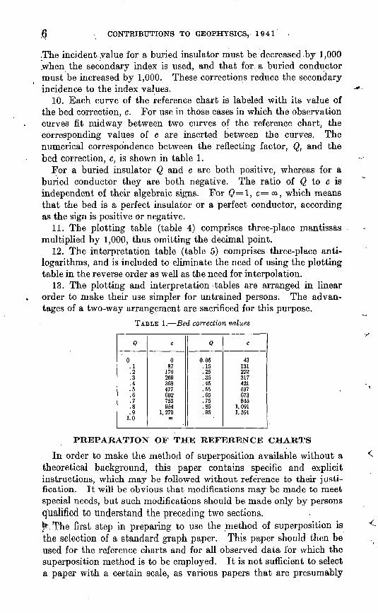
10. Each curve of the reference chart is labeled with its value of the bed correction, c. For use in those cases in which the observation curves fit midway between two curves of the reference chart, the corresponding values of c are inserted between the curves. The numerical correspondence between the reflecting factor, Q, and the bed correction, c, is shown in table 1.

For a buried insulator Q and c are both positive, whereas for a buried conductor they are both negative. The ratio of Q to c is independent of their algebraic signs. For Q=l, c= °°, which means that the bed is a perfect insulator or a perfect conductor, according as the sign is positive or negative.

11. The plotting table (table 4) comprises three-place mantissas multiplied by 1,000, thus omitting the decimal point.

12. The interpretation table (table 5) comprises three-place anti- logarithms, and is included to eliminate the need of using the plotting table in the reverse order as well as the need for interpolation.

13. The plotting and interpretation tables are arranged hi linear order to make their use simpler for untrained persons. The advan tages of a two-way arrangement are sacrificed for this purpose.

TABLE 1. Bed correction values

Q

0.1.2.3.4.5.6.7.8.9

1.0

c

087176269368477602753954

1,27901

Q

0.05.15.25.35.45.55.65.75.85.95

c

43131222317421537673845

1,0911,591

PREPARATION OF THE REFERENCE CHARTS

In order to make the method of superposition available without a theoretical background, this paper contains specific and explicit instructions, which may be followed without reference to their justi fication. It will be obvious that modifications may be made to meet special needs, but such modifications should be made only by persons qualified to understand the preceding two sections. ^.The first step in preparing to use the method of superposition is the selection of a standard graph paper. This paper should then be used for the reference charts and for all observed data for which the superposition method is to be employed. It is not sufficient to select a paper with a certain scale, as various papers that are presumably

INTERPRETATION. OF EARTH-RESISTIVITY CURVES 7

similar may differ by noticeable amounts when superposed. Also, as many graph papers are not interchangeable as to edges, the standard sheets should always be used in the same position.

After the choice of paper has been made, the reference curves may be plotted from tables 2 and 3. In each of these tables the first column lists the horizontal coordinate, Ht, to be used in plotting. Each of the other sets of columns (separated by paraUel rules) con tains the data for a single curve, the value of c for that curve being given at the top of each column. The intermediate values of c, to be inserted between the curves, may be obtained from table 1. In each column, opposite its value of Ht is the value of the vertical coordinate, Vt, for the curve.

To reproduce the curve shown in plates 1 and 2, the values in tables 2 and 3 should be plotted on the scale 1 inch= 100 units, so that only 12 inches of the horizontal scale is needed. The values in the tables are given to a tenth of a unit, to permit their use for other purposes, but the last figure cannot be used in plotting, as the unit figure corresponds to a hundredth of an inch. In the tables the values are listed so that no two curves, shall approach each other by less than 10 units, or a tenth of an inch, no curve shall approach within this distance of the base line, and no curve shall depart from the base line by more than 1,000 units, or 10 inches. The resulting curves are adequate for all ordinary purposes.

In plotting the points, place a sheet of the graph paper over a sheet of blank paper, preferably a heavy drawing paper, so fastened that the two sheets cannot slide relatively to each other. The points should be plotted with a steel needle held vertically, so as to prick through the drawing paper. Also prick through the drawing paper, at the points (0, 0), (500, 0), (1,200, 0), (0, .1,0.00), (500, 1,000) and (1,200, 1,000),

After the points have been plotted, the two sheets should be re moved. On the graph paper, the curves should be drawn in for reference and the straight lines (0, 0) (1,200, 0), (0, 1,000) (1,200, 1,000), and (500, 0) (500, 1,000) drawn. The vertical line is the depth index. On the chart for buried insulators the bottom line is the "resistivity index," and the top line is the "secondary index." On the chart for buried conductors the top line is the resistivity index and the bottom line is the secondary index. It is a simple matter to distinguish the horizontal lines, as the curves always converge to the resistivity index at the left. At the end of each curve write the value of the bed correction, c, appearing at the head of the column in the table. Between each two curves, far enough to the left to avoid confusion, write the intermediate values of c, as obtained from table 1, between the proper curve values of c. Be sure to include the alge braic sign with each value of c.

287344 41 -2

8

TABLE 2. Reference chart coordinates for buried insulator

0255075

inn1UU

125150175

200991£i£iij

250275

300325350375

400425450475

500525550575

600625650675

700725750775

800825850875

900925950975

1,0001,0251,0501,075

1,1001,1251,1501,175

1,200

+ 00

11.313.315.618.3

21.425.029.133.8

39.245.452.360.1

68.978.689.4

101.3

114.3128.4143.7160.0

177.4195.8215.1235.3

256.3278.0300.4323.3

346.6370.3394.3418.6

443.0467.6492.4517.2

542.0566.9591.9616.9

641.9666.9691.9716.9

741.9766.9791.9816.9

841.9

+1,279

78.388.8

100.3112.8126.2140.6

156.0172.3189.5207.4

226.0245.2265.0285.3

305.9326.8347.9369.2

390.5411.9433.3454.7

476.0497.2518.2539.1

559.8580.4600.8621.0

641.0660.8680.4699.8

718.9

+954

34 439i745.7

52.459.968.277.4

87.598.4

110.2122.9

136.5150.9166.1181.9

198.4215.4233.0250.9

269.1287.6306.2324.9

343.7362.4381.1399.7

418.1436.3454.3472.1

489.7507. 0524.0540.7

557.1573.3589.2604.7

619.9

+753

66.7

75.484.995.2

106.2

118.0130.6143.9157.8

172. 2187.1202.5218.2

234.2250.3266.6283.0

299.4315.7331.9347.9

363.8379.4394.8409.9

424.7439.3453.5467.4

480.9494.1506.9519.4

531.5

+602

11.713.615.918.5

21.59A Q £f±, a28.833.1

38.043.549.656.4

63.871.980.790.1

100.2111.0122.4134.3

146.7159.6172.9186.5

200.3214.2228.3242.4

256.4270.4284.3298.0

311.5324.7337.7350.4

362.8374.9386.6398.0

409.0419.7430.0440.0

449.6

+477

46.4

52.559.366.674.5

82.991.9

101.5111.5

121.9132.7143.9155.3

166.9178.7190.5202.4

214.2226.0237.6249.0

260.2271.2282.0292.4

302.5312.3321.8331.0

339.8348.3356.4364.2

371.7

+368

18.621.5

24.728.332.336.7

41.647.052.859.1

65.973.280.988.9

97.3106.1115.2124.5

133.9143.4153.0162.7

172.3181.8191.2200.4

209.4218.2226.8235.1

243.1250.8258.3265.4

272.2278.7284.9290.8

296.3

+269

30.934.939.344.1

49.254.760.566.6

73.079.786.693.6

100.8108.1115.5122.9

130.2137.5144.6151.6

158.5165.2171.6177.8

183.8189.5195.0200.2

205.1209.8214.3218.5

222.5

+176

10.5

12.113.815.818.0

20.423.126.129.3

32.736.440.344.4

48.753.358.062.8

67.772.777.782.7

87.792.697.4

102.2

106.9111.4115.7119.9

123.9127.7131.31317

138.0141.0143.8146.5

149. 1

+87

10.111.513.014.6

16.318.120.122.2

24.426.729.131.6

34.136.639.241.8

44.446.949.451.8

54.256.558.760.8

62.864.766.668.3

69.971.372.774.0

75.2

INTERPRETATION OF EARTH-RESISTIVITY CURVES

TABLE 3. Reference-chart coordinates for buried conductor

\« H'\50 75

100 125 150 175

200225250275

300325350375

400425 450 475

500 525 550 575

600 625 650

' 675

700 725 750775

800 825 850 875

900 925 950 975

1,0001,0251,050-1,075

1,1001,1251,1501,175

1,200

CO

988.2 986.2

983.8 981.0 977.7 974.0

969.7964.7958.9952.3

944.8936.1926.3915.2

902.6888.4 872.5 854.6

834.6 812.4 787.7 760.4

730.2 697.1 660.7 620.9

577.3 530.0 478.6 422.8

362.5 297.2 226.8 151.3

70.1

-1, 279

899.5 885.3 869.4

851.8 832.2 810.6 786.8

760.7 732.2 701.3 667.8

631.7 593.0 551.6 507.7

461.5 412.9 362.3 310.2

256.8 202.8 149.4 96.5

45.9

-954

955.3948.4940.6931.8

921.8910.6 898.1 884.1

868.7 851.7 832.9 812.4

790.1 765.9 739.8 711.8

681.9 650.2 616.9 582.0

545.8 508.5 470.6 432.4

394.4 356.9 320.5 285.7

253.2223.3196.2172.2

151.3133.3117.9105.2

94.6

-753

921.6 910.8 898.8

885.5 870.9 854.9 837.4

818.5 798.2 776.5 753.3

728.7 702.9 676.1 648.4

620.0 591.1 562.0 533.2

504.9 477.3 450.9 426.0

402.9381.7362.6345.6

330.7317.8306.8297.5

289.6

-602

981.2978.2974.7970.7

966.1960.9955.0948.4

941.0932.7 923.5 913.3

902.1 889.8 876.4 861.8

846.0 829.2 811.5 792.7

772.8 752.1 730.8 708.9

686.6 664.2 641.9 619.9

598.4 577.8 538.1 539.6

522.4506.6492.4479.7

468.4458.5450.1442.8

436.3

-477

943.8 936.2 927.8

918.6 908.5 897.5 885,7

873.1 859.6 845.3 830.3

814.6 798.4 781.7 764.7

747.5 730.3 713.3 696.6

680.4 664.9 650.2 636.3

623.4611.6600.8591.1

582.4574.7568.0562.1

557.0

-368

977.1973.6969. 7965.3

960.4954.9 948.9 942.3

935.0 927.0 918.4 909.2

899.4 888.9 877.9 866.4

854.4 842.0 829.4 816.6

803.8 791.0 778.4 766.1

754.1 742.6 731.7 721'. 5

712.0703.2695.1687/8

681.2675.3670.1665.5

661.3

-269

966.1 961.6 956.7

951.3 945.4 939.1 932.3

925.1 917.5 909.5 901.2

892.6 883.8 874.8 865.7

856.6 847.6 838.7 830.0

821.6 813.6 806.0 798.8

792.0785.7779.9774.7

769.9765.6761.7758.2

765.0

-176

989.9

988.3986.6984.7982.5

980.0977.3 974.3 971.0

967.5 963.7 959.6 955.1

950.4 945.5 940.3 935.0

929.5 923.8 918.0 912.2

906.5 900.8 895.2 889.8

884.5 879.4 874.5 869.9

865.6861.6857.9854.5

851.3848.4845.8843.4

841.4

-87

990.0988.6 987.1 985.5

983.7 981.8 979.8 977.6

975.3 972.9 970.4 967.8

965.2 962.5 959.7 956.9

954.2 951.5 948.8 946.2

943.7 941.2 938.8 936.6

934.5932.6930.8929.1

927.5926.0924.7923.5

922.5


The working charts should be made from the drawing paper with out drawing the curves or lines on it. If the working medium is to be tracing paper, tracing cloth, or very thin acetate sheeting, the direct side may be used for copying, using an ordinary ruling pen and opaque ink. A better medium is acetate sheeting about 0.015 inch thick. This is easily handled, can be cut to size, is transparent, is durable, and can be scratched with a needle or knife. If this medium is used, the copying should be done in reverse. To do this, use the bottom side of the drawing sheet as a guide for making the curves, and scratch the lines in the acetate with a needle or thin knife, being careful to hold the cutting tool vertical to avoid errors of parallax. The scratch should be definite but not deep enough to cause the sheet to crack. If such a medium is new to the draftsman, he should practice on small pieces until he has become familiar with the pressure needed for good results. After the curves are cut, they should be filled with opaque ink, such as ordinary waterproof drawing ink. After the ink has dried thoroughly (preferably several hours) the excess may be removed by rubbing lightly across the cuts with a slightly moistened cloth. The cloth should be wet enough to dis solve the ink from the surface without removing it from the cuts, and the pressure should be only heavy enough to attain this end. The lettering and numbering may be added to either side of the sheet ing and may also be cut, if desired. However, ordinary writing with a pen and india ink, on the direct side, will usually suffice. If the writing wears off or dims, it can be replaced without difficulty. Parallax and accuracy of location are not important for the labeling of the chart.

The resulting reference charts are illustrated in plates 1 and 2, which may be considered accurate within 2 percent or less.

THE SUPERPOSITION METHOD OF INTERPRETATION

To apply the method of superposition to the observed data, the procedure is as follows:

Step 1. PREPARE A PLOTTING SHEET. A convenient form is shown in table 6 (p. 13), which gives an example of the method. The values of the separation, a, and the apparent resistivity, pa, are taken directly from the field notes. The value of H is determined by the value of a, and the value of V is determined by the value of pa . In the values of H and V to be plotted there are four figures each. The first figure is the number of significant figures to the left of the decimal point in the observed data. The remaining three figures are obtained from the plotting table (table 4). To obtain these three figures, round the observed data to three figures without reference to the position of the. decimal point, adding ciphers if necessary. Find the resulting number


under the heading " No." in table 4. In, the next column, opposite this number under the heading "Gr.," will be found the last three figures of the value to be plotted.

.Thus, consider the value p0=6,725. The first figure of V is 4, as there are four figures to the left of the implied decimal point. To obtain the remaining figures, round 6,725 to 672. In rounding, if the fourth figure is 0, 1, 2, 3, or 4, drop all figures beyond the third. If the fourth figure is 6, 7, 8, or 9, increase the third figure by one and drop the following figures. If the fourth figure is 5 and a later figure differs from zero, in any position, increase the third figure by one and drop the following figures. If the fourth figure is 5 and there are no following figures that differ from zero either choice is equally good. In this paper the nearest even figure is selected as the third figure. Thus, 6,725 becomes 672, although 673 would be just as correct.

In table 4 we find 672 under the heading "No." and 827 opposite it, under the heading "Gr." Thus for Pa = 6,725, we have F=4,827. If 6,725 were rounded to 673, we should have F=4,828. The dif ference is negligible, as it will be usually. Similarly, if a= 5, H= 1,699, and if a=15, #=2,176.

Step 2. PLOT THE SUPERPOSITION CURVE. The table obtained in step 1 is reduced to a graph by plotting H horizontally and V ver tically, on the paper and in the units selected for the reference charts. Each observation is plotted as a center of a small circle. It is pref erable not to draw a curve through the circles, since a line connecting the points may affect the judgment of the interpreter in finding the best fit or may tend to obscure the lines of the reference chart.

Step 3. SUPERPOSE THE REFERENCE CHART .OVER THE SUPERPOSITION GRAPH. If the superposition curve rises to the right, a buried insulator is indicated, and the chart for buried insulators is used. Similarly, for a descending curve, the chart for buried conductors is used. Lay the reference chart over the superposition graph of the observed data with the depth index vertical. Slide the chart over the graph, without turning it, until the points of the graph agree with one of the curves of the reference chart, or lie midway between two such curves., Step 4. READ THE INDEX VALUES. After determining the position of "best fit," read the value of H, on the graph, directly under the "depth index" and the value of V directly under the "resistivity index." If the resistivity index does not lie over the graph, use the secondary index. For buried insulators the value under the secondary index must be decreased by 1,000 to obtain the value that would lie under the resistivity index if the graph were large enough. Similarly, for buried conductors the secondary value must be increased by 1,000 to obtain the value of the resistivity index. The depth index usually lies over the graph. Call the values under the depth and resistivity

l"2 CONTRIBUTIONS TO GEOPHYSICS, 1941

index, H0 and V0 , respectively, and list the value of c for the curve of best fit, or between the two curves determining the position of best fit.

Step 5. CONVERT THE INDEX VALUES TO INTERPRETED VALUES. To

convert the index values to interpreted values having physical sig nificance, use the interpretation table (table 5). In this conversion, H0 determines the depth, h; V0 determines the resistivity of the overburden, p0, and V0 -\-c determines the value of the bed resistivity, PJ,. The sequence of figures is determined by the last three figures, and the position of the decimal point by the first figure. Under "Gr." in table 5, find the last three figures in the index value. Immediately opposite this entry, find, under "No." the sequence. The position of the decimal point is such that the number of figures to the left of the decimal point is the same as the first figure of the index value.

In the example shown below, superposition determines the index value F0 =4,800. Under "Gr." in table 5, we find the number 800. Under "No." immediately opposite 800, we find 631. As the first figure of 4,800 is 4, there will be four figures in the result, and the value of PO is 6,310. Similarly, the index value of V0 -\-c is 5,168. The value 168 under "Gr." corresponds to 147 under "No." and as the first figure of 5,168 is 5, the bed resistivity is p 6 14,700.

The foregoing steps may be summarized as follows:1. Prepare a plotting sheet from the observed data, using the

plotting table (table 4) to convert the observed values to graph values.2. Plot the superposition points from the table of step 1, but leave

the points as separate circles, not connected.3. Superpose the observation curve and reference chart.4. Read the index values for the superposition of best fit.5. Convert the index values to depth and resistivity values, using

the interpretation table (table 5).

AN ILLUSTRATIVE EXAMPLE

To illustrate the method, consider the data given in the first two columns of table 6. From table 4, H is obtained from the value of a, and V is obtained from the value of pa . The value of V is plotted vertically, and the value of H is plotted horizontally, as shown by the circles in figure 2. Superposition of the reference chart shows that the best fit is obtained for c=+368, with the depth index H0 =3,2QQ and the resistivity index V0 =4,800. The value of V0 -\-c is 5,168. From table 5 we find that H0 corresponds to the depth ^=182, the value of V0 corresponds to the overburden resistivity p«,=6,310, and the value of V0 -\-c corresponds to the bed resistivity p 6 =14,700.

5.100

4,8003.0OO

INTERPRETATION OF EARTH-RESISTIVITY CURVES

TABLE 6. Data fqr illustrative example

13

a

120 140 160

180 200 220

240 260 280

300 320 340

360 380 400

420 440 460

480 SCO 520

540 560 580

Pa

6.725 6,900 7,075

7,425 7,450 7,800

8,275 8,365 8. 435

8,650 8,825 9,055

9,150 9,275 9,625

9,600 10, 250 10,275

10, 325 10, 375 10, 610

10, 785 11,000 11, 050

H

3,079 3,146 3,204

3,255 3,301 3,342

3,380 3,415 3,447

3,477 3,505 3,531

3,556 3,580 3,602

3,623 3,643 3.663

3,681 3,699 3,716

3,732 3.748 3,763

V

4,827 4,838 4,850

4,870 4,872 4,892

4,918 4,922 4,926

4,937 4,945 4,957

4,961 4,967 4,983

4,982 5,009 5,013

5,013 5,017 5,025

5,033 5,041 5,041

a

600 620 640

660 680 700

720 740 V60

780 800 820

840 860 880

900 920 940

960 980

1,000

Pa

11, 125 11, 385 11,100

11, 300 11, 525 11,375

11, 530 11, 560 11, 600

11,600 11,425 11, 535

11, 575 11, 600 11, 610

11, 525 11,815 11, 725

12,050 11,750 11,975

H

3,778 3,792 3,806

3,819 3,832 3,845

3,857 3,869 3,880

3,892 3,903 3,913

3,924 3,934 3,944

3,954 3,963 3,973

3,982 3,991 4,000

V

5,045 5,057 5,045

5,053 5,061 5,057

5,061 5,064 5,064

5,064 5,057 5,061

5,064 5,064 5,064

5,061 5,072 5,068

5,079 5,072 5,079

H 3,500

FIGURE 2. Superposition graph for illustrative example.

4,000

To check this interpretation, we may plot the curve

>

where Ht and Vt are corresponding values taken from table 2 in the column c=+368. To avoid unnecessary labor, we note that H extends from 3,000 to 4,000, so that Ht is needed only from 260 to 1,200. The values of H and V for the reference curve in the inter preted position are shown in table 7. This type of check is not necessary in practice and requires the ability to understand the two sections of a theoretical nature (pp. 3-6).


TABLE 7. Values of V for reference curve in position shown in figure

H,

250 275 300

325 350 375

400 425 450

475 500 525

550 575 600

625 650 675

700 725 750

H

3,010 3,035 3,060

3,085 3,110 3,135

3,160 3, 185 3,210

3,235 3,260 3,285

3,310 3,335 3,360

3,385 3,410 3,435

3,460 3,485 3,510

V

4,819 4,822 4,825

4,825 4,832 4,837

4,842 4,847 4,853

4,859 4,866 4,873

4,881 4,889 4,897

4,906 4,915 4,925

4,934 4,943 4,953

Hi

775 800 825

850 875 900

925 950 975

1,000 1,025 1, 050

' 1,075 1,100 1,125

1,150 1,175 1,200

H

3,535 3,560 3,585

3,610 3,635 3,660

3,685 3,710 3,735

3,760 3,785 3,810

3,835 3,860 3,885

3,910 3,935 3,960

V

4,963 4,972 4,982

4, 991 . 5,000 5,009

5,018 5,027 5,035

5,043 5,051 5,058

5,065 5,072 5,079

5,085 5,091 5,096

It will be noted that the observations fall below the reference curve at the upper end, indicating that a deeper contact is beginning to affect the observations. Except for the ends, the reference curve agrees well with the observations, indicating a contact at a depth of about 182 feet. For this portion of the curve, all the materials above this contact are equivalent to a homogeneous, isotropic material of resistivity 6,310 ohm-centimeters, and all the materials below the contact are equivalent to one of resistivity 14,700 ohm-centimeters.

If the superposition leads to a fit intermediate between two curves on the chart, and it is desired to check the interpretation as explained above, we may use the mean of the values given in the table for the adjacent values. Although this is not justified by theory, it is suf ficiently reliable for practical purposes.

DISCUSSION

The purpose of this paper is to present the method of superposition for interpreting data on electrical resistivity obtained where bedrock is covered by a single overburden, in a form that permits the routine work to be performed by persons not trained in geophysics or advanced mathematics. Except for the se'ctionb on pages 3-6 (see footnote 2), which may be omitted by such readers, the instructions and remarks have been made specific, and no attempt has been made to justify, correlate, or expand the details.

Numerous aspects of the subject have been omitted intentionally. Some of these are discussed briefly in this section.

INTERPRETATION: OF :EARTH-RESISTIVITY; CURVES 15

: Applicability of the partition method. In the partition method of measuring'-electrical resistivity 6 the potentials of the points C and D, figure 1, are measured with reference to a stake midway between them. The only effect of this is to double the constant in the formula, so that the apparent resistivity obtained from the field operations occurs as two values, each of which may be treated as in the simple case. Hence no modification is needed for the superposition, as the disturbing factor is unchanged theoretically.

Modification oj the measuring system. The system of making the measurements may be modified to suit the observer, but such a modification usually will require new tables and new reference charts. If the system departs from the Wenner system, except for the par tition method and a few others, new tables should be calculated di rectly from the basic tables.7

. Reliability. The reliability of the superposition method is affected by many factors. It should be remembered that the assumed con ditions represent idealized circumstances and that the conclusions will be approximate to the same degree as the actual conditions may.be represented by the theoretical picture.

Homogeneity and isotropism. In the theoretical development the overburden and bed are each assumed to be homogeneous and isotropic. In nature such a condition is seldom found. However, a mixture of geologic materials may possess a degree of homogeneity and isotropism sufficient for purposes of study. Thus, a regular distribution of approximately equal-sized pebbles in sand is not homogeneous if the unit volume is 1 cubic centimeter, but may be considered homogeneous if the unit volume is 1 cubic meter. In this sense a material is homogeneous and isotropic if a unit cube has throughout the same electrical resistivity independently of the loca tion and orientation. If measurements are made 100.meters apart, irregularities in various samples having a unit volume of 1 cubic meter may often be neglected, unless there exists a definite trend or sharp change in character within the region of measurement.

Average resistivity. In view of the preceding paragraph, it is possible for a stratum to have an average resistivity that is not the actual resistivity of any material contained in it. Thus, if the average resistivity of a stratum does not change too much as the elec trode separation increases, we may consider that stratum homo geneous. As an example, a stratum composed of alternating thin layers of shale and sandstone would display an average resistivity intermediate between those for these two materials and differing little for different parts of the-stratum or different electrode spacings.

Lee, F. W., and Swartz, J. H., Eesistivity measurements of oil-bearing beds: U. S. Bur. Mines Tech. Paper 488,1930. .. . ...

i Roman, Irwin, op. cit. (TJ. S. Bur. .Mines, \Tech. Paper 502). . . . ;-...... .:

16 '.".. .CONTRIBUTIONS;TO GEOPHYSICS, 19 41 .

Such a stratum would be homogeneous in the sense here required; accordingly, there need not be a true lithologic homogeneity or isotropism in either the overburden or the bedrock to make the method applicable. The requirements are that the average resistivity of each remains fairly constant as the electrode separation is increased, and that there shall be an approximately horizontal contact above and below which the average resistivities are definitely distinct.

Partial superposition. -If the entire superposition graph can be made to agree with a curve on the reference chart, it is reasonable to conclude that the idealized conditions have been approximated in the region surveyed and that the predicted depth should agree closely with the actual depth to the surface of contact. In many places, however, the idealized conditions do not approximate the actual conditions sufficiently to make a complete fitting possible, and it must be inferred that there are two or more surfaces of contact. The theoretical problem has been solved for the case of two horizontal contacts,8 but these theoretical results have not been reduced to curves of reference. A few isolated examples of such curves have been obtained by mechanical or approximate methods. One system atic attempt to plot such curves was made by Wetzel and McMurry, 9 but the curves they give are not arranged conveniently for super position and are not spaced closely enough for quantitative interpre tation. An attempt to apply the two-layer curves to more than two layers was made by Hummel, 10 using an approximate method, and the same method was applied by Watson and Johnson. 11

Such curves obviously do not fall in the assumed group, but it is sometimes possible to fit the curves in sections and consider the interpreted depths as indicators; thus, a layer at 500 feet may lead to an interpreted depth of 200 or 900 feet, which is evidently not a good interpretation. If, however, consecutive curves are similar and lead to consistent changes in the depth of the marker, it is often possible to determine the character of the contact by this simple means for example, to identify a certain type of curve family with an anticline, or to determine the location and direction of throw of a fault by changes in consecutive curves. Although both of these conclusions may be numerically wrong on the basis of well logs and geologic correlation, they may show that such qualitative information can be .very valuable in selecting a location for drilling or in explaining un-

> Koman, Trwin, Thn calculation of electrical resistivity for a' region underlying two uniform layers: Terrestrial Magnetism and Atmospheric Electricity, vol. 38, No. 2, pp. 117-140, June 1933; No. 3, pp. 185- 202, September 1933. This paper contains additional references.

» Wetzel, W. W., and McMurry, H. V., A set of curves to assist in the interpretation of the three-layer resistivity problem: Geophysics, vol. 2, No. 4, October 1937.

10 Hummel, J. N., A theoretical study of apparent resistivity in surface potential methods: Am. Inst. Min. Met. Eng., Geophysical prospecting, 1932, pp. 407-422.

" Watson, K. J., and Johnson, J. F., On the extension of the two-layer methods of interpretation of earth- resistivity data to three and more layers: Geophysics, vol. 3, No. 1. pp. 7-21,1938.


expected performance in wells. Such information can also prevent costly development work in areas of unfavorable structure and can often furnish information in areas for which no quantitative data are available or in which the projection of geologic data is not safe.

Where there is only partial superposition, the interpreter has a simple method of performing a task for which no better tools exist, but he must remember that the conclusions are less accurate and he must draw Ins inferences accordingly. When the method has been, extended, he can check his interpretations for those areas that may still be of interest, but until better methods are available, partial, superposition of the single overburden curves may be useful.

In many regions partial superposition is not applicable. Unless- 'successive layers are reasonably thick, the deeper layers will affect the curve of apparent resistivity to such an extent that no fit of im portance can be made; thus, if the character of the observation curve changes after a few separations, it is not possible to approximate a. superposition. Specifically, in one region- surveyed the material consisted of alternate layers of clay and sand only a few feet thick, and each layer affected so large a part of the resistivity curve that it was impossible to identify the effects of the individual beds. Such curves must be studied in reference to their character or qualitatively. No improvement could be expected through theoretical extensions of the superposition method.

Only experience and judgment will enable the geophysicist to deter mine whether it is advisable to apply the method of superposition to the interpretation of a specific set of data, or to place great reliance on the conclusions. If he decides that it is advisable to apply the method, the routine analysis may be performed by a subordinate.

Uniqueness. For some resistivity curves the data are such that the interpreter has little freedom in fitting the observations to the reference chart. If so, independent interpreters will obtain values of depth and resistivity differing only slightly from each other, and little experience is needed to obtain reliable interpretations. As an ex-

. ample, the writer recalls a curve that was fitted by him and an assist ant, independently. The superposition showed a contact at a depth that could not be much less than 34 feet nor much greater than 35 feet; however, this interpretation was considered impossible by the geologists who had studied the area, as the ground cover was glacial drift to a depth of more than 100 feet. Accordingly, the interpreta tion was considered erroneous, and the curves were returned to the files. About 6 months later the curves were superposed again, with out reference to the former interpretations. The conclusions were the- same, and the curves were jeturned to the files a second time. Several years later a hole was drilled in this area by a driller who had no- knowledge of the resistivity interpretation. When a depth of about-

18 V ' CONTRIBUTIONS TO GEOPHYSICS, 1941; j

34 feet was reached, the driller noticed that progress was impeded. He probed for boulders and finally resorted to dynamite. A lens of "hardpan" was the contact which the interpretations had detected-, contrary to the geologic inferences of the region.

The slopes of some curves are such as to determine the curve of fit definitely, but the curvature is so slight that there is considerable freedom in determining the overlapping portions of the reference curve and observation graph. Both depth and resistivity are then subject to variation in interpretation, but interdependent^. This difficulty can be avoided only by extending the observations to include the more curved portions of the graphs. Inasmuch as many com binations of depth and resistivity may lead to similar curves differently placed on the graph sheet, such lack of uniqueness is due to the geologic and experimental conditions and is not a fault of the method of super position. The cause is an insufficiency of data.

It may happen that several curves on a reference chart can be superposed equally well. This difficulty is also due to insufficiency of data. There is no way to avoid it except by the addition of more and better data.

In general, the better the superposition the more nearly unique will be the interpretation. The shorter the section of fit the more freedom will there be in the interpretation.

o

n

-4-

The use of the subjoined mailing label to return

this report will be official business, and no

postage stamps will be required

UNITED STATES PENALTY FOR PRIVATE USE TO AVOID DEPARTMENT OF THE INTERIOR PAYMENT OF POSTAGE, $300

GEOLOGICAL. SURVEY

OFFICIAL BUSINESS

This label can be used only for returning official publications. The address must not be changed.

GEOLOGICAL SURVEY,

WASHINGTON, D. C.