SUPEROXYGENATION: ANALYSIS OF OXYGEN TRANSFER …

SUPEROXYGENATION: ANALYSIS OF OXYGEN TRANSFER DESIGN

PARAMETERS USING HIGH PURITY OXYGEN AND A PRESSURIZED

AERATION COLUMN

by

TYLER WILLIAM BARBER

B.Sc. California Polytechnic State University, San Luis Obispo, California, U.S.A.,

2011

A THESIS SUBMITTED IN PARTIAL FULFILLMENT OF THE

REQUIREMENTS FOR THE DEGREE OF

MASTER OF APPLIED SCIENCE

in

The Faculty of Graduate and Postdoctoral Studies

(Civil Engineering)

THE UNIVERSITY OF BRITISH COLUMBIA

(Vancouver)

August, 2014

© Tyler William Barber

ii

Abstract

Supplying oxygen to water via the physical process of aeration is the most widely used water

treatment technology. It supports microbial growth in water and wastewaters by introducing

dissolved oxygen to the water, stabilizing organic matter and providing the necessary oxygen for

many other aquatic species to survive. There exists the potential for much improvement in

aeration techniques, which can account for 60 percent of the energy required for water treatment.

This research aimed to analyze one such technique that has limited research of this magnitude,

aerating water under high pressures with high-purity oxygen. Increasing the partial pressure of

oxygen in the aeration gas, by way of Henry's law, increases the saturation concentration of the

water and, thus, several aeration design parameters. The parameters required for aeration design

and sought after in this research are: the mass transfer coefficient (KLa), saturation concentration

(C*sat), standard oxygen transfer rate (SOTR), standard aeration efficiency (SAE), and the

standard oxygen transfer efficiency (SOTE). This research compared the obtained design values

under gauge pressures of 0, 50, 100, 150, and 200 kPa using air and Pressure Swing Adsorption

(PSA) oxygen in an 18.5 foot (5.6 meter) aeration column, allowing for comparative analysis of

the design parameters for aeration. Results show that, with increasing pressure for both air and

PSA oxygen: KLa decreases, C*sat increases; however, at a rate other than predicted by Henry's

law, the SOTR remains constant, the SAE decreases, and the SOTE increases. Between air and

PSA oxygen, PSA was found to have a slightly larger KLa, larger C*sat, larger SOTR, lower SAE,

and a higher SOTE.

iii

Preface

This thesis is ultimately based on theorized conjectures made by Dr. Richard Speece in

collaboration with Drs. Ken Ashley and Don Mavinic. This thesis provides experimental data

and results for said conjectures.

The manifold board and PSA unit used in the research were the same units used in Ashley (2002)

research, with the design and construction of the manifold board provided by Point Four

Systems, Inc.

Design, placement, and construction of the D.O. probes, RIU's, and pump within the column was

completed by the author, Tyler William Barber. Additionally, the process for monitoring

effervescence, chemical mixing, and calibration procedure was designed by the author.

The data analysis of the D.O.-versus-time data was completed using a macro-enabled Excel

spreadsheet provided by Dr. Michael Stenstrom, author of the ASCE standard for oxygen

transfer. The analysis of data with the spreadsheet was completed by the author.

iv

Table of Contents

Abstract ........................................................................................................................................... ii

Preface............................................................................................................................................ iii

Table of Contents ........................................................................................................................... iv

List of Tables ................................................................................................................................ vii

List of Figures ................................................................................................................................ ix

Nomenclature .................................................................................................................................. x

Acknowledgements ...................................................................................................................... xiii

1 Introduction ............................................................................................................................. 1

1.1 Literature Review of Aeration and Superoxygenation ..................................................... 1

1.1.1 Aeration Background ................................................................................................ 1

1.1.2 Aeration Using Pure Oxygen .................................................................................... 3

1.1.2.1 High Purity Oxygen Activated Sludge Systems ................................................ 3

1.1.2.2 High Purity Oxygen Hypolimnetic Aeration Systems ...................................... 4

1.1.2.3 High Purity Oxygen in Aquaculture .................................................................. 6

1.1.3 Superoxygenation ..................................................................................................... 6

1.2 Rationale for Current Research ........................................................................................ 8

1.3 Objectives ......................................................................................................................... 9

2 Equipment and Methods ....................................................................................................... 10

2.1 System Design ................................................................................................................ 10

2.1.1 Aeration Column ..................................................................................................... 10

2.1.2 Air and Oxygen Flow Measurement ....................................................................... 12

2.1.3 Oxygen and Air Source ........................................................................................... 14

2.1.4 Water Source and Volume Measurement ............................................................... 14

2.1.5 D.O. Probes ............................................................................................................. 15

v

2.1.6 Data Logger ............................................................................................................ 16

2.2 Experimental Design ...................................................................................................... 19

2.2.1 Experimental Groups - Superoxygenation .............................................................. 19

2.2.2 Experimental Groups - Deoxygenation .................................................................. 19

2.3 Experimental Procedure ................................................................................................. 21

2.3.1 Superoxygenation Procedure .................................................................................. 21

2.3.1.1 Chemical Deoxygenation Procedure ............................................................... 22

2.3.1.2 Probe Calibration ............................................................................................. 22

2.3.1.3 Termination of Experiments ............................................................................ 25

2.3.2 Effervescence Deoxygenation Procedure ............................................................... 25

2.4 Parameter Estimation ..................................................................................................... 26

2.4.1 Power Estimation .................................................................................................... 30

2.5 Statistical Analysis ......................................................................................................... 32

3 Results ................................................................................................................................... 33

3.1 Superoxygenation ........................................................................................................... 33

3.1.1 Air ........................................................................................................................... 33

3.1.2 PSA Oxygen............................................................................................................ 42

3.1.3 Air-versus-PSA Oxygen ......................................................................................... 52

3.2 Effervescence ................................................................................................................. 57

3.3 Quality Control ............................................................................................................... 63

3.3.1 Winkler Titration .................................................................................................... 63

3.3.2 Results ..................................................................................................................... 64

4 Discussion ............................................................................................................................. 66

4.1 Gas Transfer Theory....................................................................................................... 66

4.1.1 Applications of Gas Transfer Theory ..................................................................... 68

vi

4.1.1.1 Oxygen Saturation Concentration ................................................................... 68

4.1.1.2 Oxygen Transfer Coefficient ........................................................................... 69

4.1.1.3 Dissolved Oxygen Concentration in Bulk Liquid ........................................... 70

4.1.1.4 Factors Affecting Effervescence ..................................................................... 70

4.2 Effect of Pressure on Mass Transfer Coefficient ........................................................... 70

4.2.1 Effect of Differing Gas Purities on Mass Transfer Coefficient .............................. 72

4.3 Effect of Pressure on Saturation Concentration ............................................................. 74

4.3.1 Effect of Henry's Constant ...................................................................................... 74

4.4 Effect of Pressure on SOTR ........................................................................................... 76

4.5 Effect of Pressure on SAE .............................................................................................. 76

4.6 Effect of Pressure on SOTE ........................................................................................... 77

4.7 Effervescence ................................................................................................................. 78

4.7.1 Scenario A ............................................................................................................... 79

4.7.2 Scenario B ............................................................................................................... 79

4.7.3 Scenario C ............................................................................................................... 79

4.7.4 Scenario D ............................................................................................................... 79

4.8 Superoxygenation Practicality........................................................................................ 80

5 Conclusions and Recommendations ..................................................................................... 82

5.1 Conclusions .................................................................................................................... 82

5.2 Recommendations .......................................................................................................... 84

References ..................................................................................................................................... 85

Appendix 1: Sample D.O. spreadsheet ......................................................................................... 89

vii

List of Tables

Table 2.1: Superoxygenation experimental design ....................................................................... 19

Table 2.2: Effervescence experimental design ............................................................................. 20

Table 2.3: Power calculations for superoxygenation treatments. ................................................. 31

Table 3.1: Aeration results for oxygen source from air at 0 kPa (0 atm) - including all values. .. 33

Table 3.2: Aeration results for oxygen source from air at 0 kPa (0 atm) - omitting outliers. ....... 33

Table 3.3: Aeration results for oxygen source from air at 50 kPa (0.5 atm) - including all values.

....................................................................................................................................................... 34

Table 3.4: Aeration results for oxygen source from air at 50 kPa (0.5 atm) - omitting outliers. .. 34


....................................................................................................................................................... 35

Table 3.6: Aeration results for oxygen source from air at 100 kPa (1.0 atm) - omitting outliers. 35


....................................................................................................................................................... 36

Table 3.8: Aeration results for oxygen source from air at 150 kPa (1.5 atm) - omitting outliers. 36


....................................................................................................................................................... 37

Table 3.10: Aeration results for oxygen source from air at 200 kPa (2.0 atm) - omitting outliers.

....................................................................................................................................................... 37

Table 3.11: Aeration results for oxygen source from PSA at 0 kPa (0 atm) - including all values.

....................................................................................................................................................... 43

Table 3.12: Aeration results for oxygen source from PSA at 0 kPa (0 atm) - omitting outliers. . 43

Table 3.13: Aeration results for oxygen source from PSA at 50 kPa (0.5 atm) - including all

values. ........................................................................................................................................... 44

Table 3.14: Aeration results for oxygen source from PSA at 50 kPa (0.5 atm) - omitting outliers.

....................................................................................................................................................... 44


values. ........................................................................................................................................... 45

Table 3.16: Aeration results for oxygen source from PSA at 100 kPa (1.0 atm) - omitting

outliers........................................................................................................................................... 45

viii


values. ........................................................................................................................................... 46


outliers........................................................................................................................................... 46


values. ........................................................................................................................................... 47


outliers........................................................................................................................................... 47

Table 3.21: Air effervescence at 50 kPa (0 atm). ......................................................................... 58

Table 3.22: Air effervescence at 100 kPa (1.0 atm). .................................................................... 59



Table 3.25: PSA oxygen effervescence at 50 kPa (0.5 atm). ........................................................ 60

Table 3.26: PSA oxygen effervescence at 100 kPa (1.0 atm). ...................................................... 61



Table 3.29: Winkler titration D.O. values..................................................................................... 64

Table 3.30: Expected D.O. in column without accounting for effervescence. ............................. 65

Table 3.31: Expected D.O. in column accounting for 35% effervescent loss. ............................. 65

Table 4.1: Log-Deficit versus Non-Linear Regression method for PSA at 50 kPa. ..................... 73

Table 4.2: Log-Deficit versus Non-Linear Regression method for air at 50 kPa. ........................ 73

ix

List of Figures

Figure 2.1: Test column schematic (not to scale). ........................................................................ 11

Figure 2.2: Manifold board schematic. ......................................................................................... 13

Figure 2.3: RIU connection schematic, connected with an RS 485 PC Communication Cable. .. 17

Figure 2.4: Manifold board and RIU configuration. ..................................................................... 18

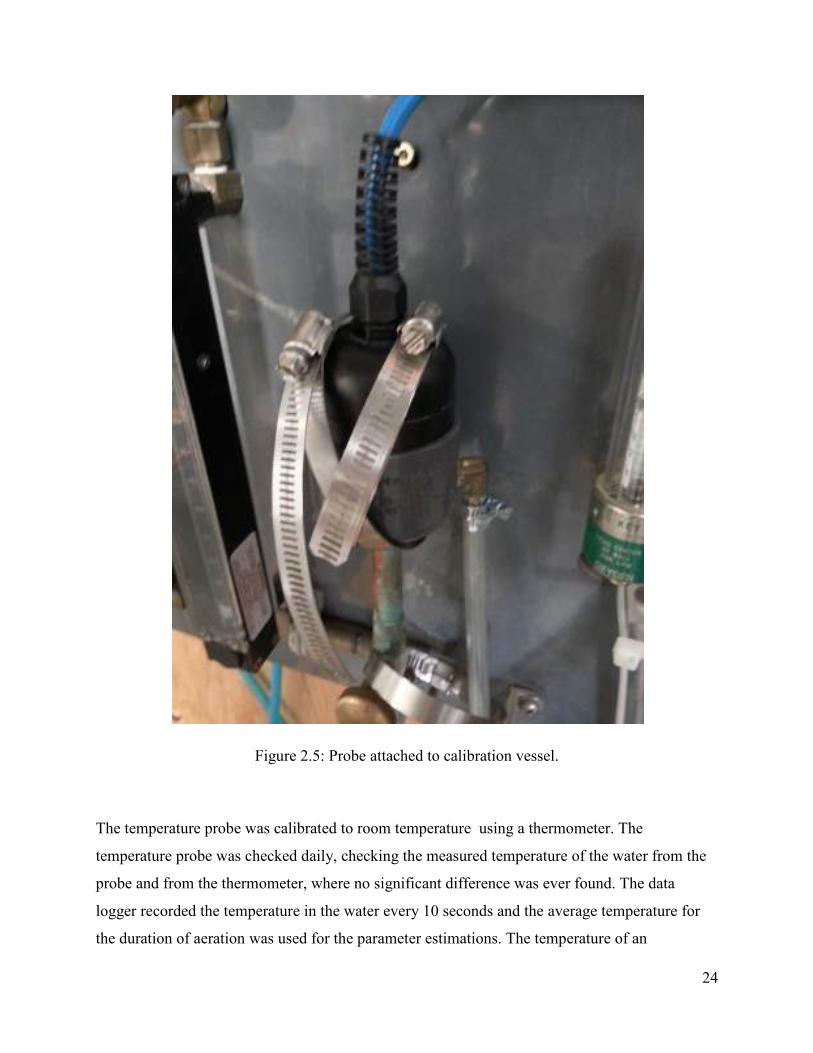
Figure 2.5: Probe attached to calibration vessel. .......................................................................... 24

Figure 3.1: Overall mass transfer coefficient for air. .................................................................... 38

Figure 3.2: Saturation concentration for air. ................................................................................. 39

Figure 3.3: Air standard oxygen transfer rate. .............................................................................. 40

Figure 3.4: Air standard aeration efficiency. ................................................................................ 41

Figure 3.5: Air standard oxygen transfer efficiency. .................................................................... 42

Figure 3.6: Overall PSA oxygen mass transfer coefficient........................................................... 48

Figure 3.7: PSA oxygen saturation concentrations. ...................................................................... 49

Figure 3.8: PSA oxygen standard oxygen transfer rate. ............................................................... 50

Figure 3.9: PSA oxygen standard aeration efficiency. ................................................................. 51

Figure 3.10: PSA oxygen standard oxygen transfer efficiency. ................................................... 52

Figure 3.11: Overall mass transfer coefficient for air and PSA oxygen. ...................................... 53

Figure 3.12: Saturation concentration for air and PSA oxygen. ................................................... 54

Figure 3.13: Standard oxygen transfer rate for air and PSA oxygen. ........................................... 55

Figure 3.14: Standard aeration efficiency for air and PSA oxygen. ............................................. 56

Figure 3.15: Standard oxygen transfer efficiency for air and PSA oxygen. ................................. 57

Figure 3.16: Air effervescent loss for scenarios A-D. .................................................................. 60

Figure 3.17: PSA effervescent loss for scenarios A-D. ................................................................ 62

Figure 4.1: Concentration gradient from gas-liquid interface (Csat) to bulk liquid (CL). .............. 67

x

Nomenclature

A Absorbing surface area of air bubbles (m2)

Atm Atmospheres, unit of measure for pressure

ASCE American Society of Civil Engineers

A/V a, the interfacial area through which mass transfer of oxygen occurs per

volume of water aerated, specific to particular aeration systems (m2/m

3)

BOD Biochemical Oxygen Demand (mg/L)

C*sat Saturated dissolved oxygen concentration (mg/L). Can be obtained from

experiments or air-water dissolved oxygen saturation tables.

C*sat20 Saturated dissolved oxygen concentration at 20°C (mg/L)

Ci Dissolved oxygen concentration at gas bubble interface, assumed to be

saturation concentration (mg/L)

CL Average concentration of dissolved oxygen in the bulk liquid (mg/L)

CSV Comma Separated Variable, format for data logging.

DBCA Downflow Bubble Contact Aeration

D.O. Dissolved Oxygen (mg/L)

e Compressor efficiency, assumed to be 0.80 in adiabatic compression

g grams, unit of weight measurement

k Ratio of specific heat capacities (CP/CV) for air and oxygen in adiabatic

compression formula

KL Liquid film coefficient (m/hr)

KLa Overall oxygen mass transfer coefficient (hr-1

)

KLaT Overall oxygen mass transfer coefficient at temperature T°C (hr-1

)

xi

KLa20 Overall oxygen mass transfer coefficient at 20°C (hr-1

)

kPa Kilopascal, unit of measure for pressure (1.0 Atm = 101.325 kPa = 14.7

psi)

kW Kilowatt, a unit of power measurement

L Liters, unit of volume measurement

min Minute, unit of time measurement

O2 Diatomic oxygen

p Pressure, gauge or absolute

Pw Power input from adiabatic compression

psia Pounds per square inch absolute (includes atmospheric pressure, 14.7 psi)

psig Pounds per square inch gauge (excludes atmospheric pressure, 14.7 psi)

R Engineering gas constant for air/oxygen (8.314 kJ/k mol °K)

RIU Remote Interface Unit, displays dissolved oxygen concentrations from

probes

SCFM Standard cubic feet per minute, air flow rate

SAE Standard aeration efficiency (g O2/kWhr)

SOTE Standard oxygen transfer efficiency (%)

SOTR Standard oxygen transfer rate (g O2/hr)

Saturation A maximum attainable dissolved oxygen concentration for a given

temperature and pressure of water.

Supersaturation When conditions rapidly change (i.e, T or P) to reduce the saturation

concentration of the water; however there still exists concentrations above

the new saturation; the water is supersaturated for a finite amount of time.

xii

t Time (hr)

T Temperature (°C or °K)

V Volume of water aerated (m3)

w Weight of air flow (kg/s)

WO2 Mass flow rate of oxygen in the gas stream (g O2/hr)

XSLX Excel file name for saved data

xiii

Acknowledgements

This thesis was completed with the excitement of knowing that research of this magnitude had

never been completed before for aeration. Having the opportunity to do work of this importance

was more than I could have ever hoped for in obtaining my Master's degree. A special thanks to

my advisors Drs. Don Mavinic and Ken Ashley for the opportunity to work on this project and

for their mentorship in the world of aeration and many hot chocolates along the way. Ken

Christison and Barry Chilibeck for allowing the research to be conducted at Northwest Hydraulic

Consultants and for the access to everything that I could need in the NHC lab. Paul Sampson

who developed much of the ideas and fabrication for this project, i.e., how to make the lid air-

tight in the column, how to pressurize the probes for calibration, construction of the column, and

any other advice given while conducting experiments. Paula Parkinson and Tim Ma in the UBC

Environmental Engineering lab, for the help they provided in obtaining all the tools I needed for

this project. My colleagues in the UBC PCWM group who provided advice for many issues I had

along the way. None of this would have been possible without the support of my family:

grandparents, dad, uncle, mom, brothers, and all my other relatives who made Vancouver a new

home for me. They helped me financially, motivated me, and gave me much needed breaks from

work along the way. And finally to my great-grandpa whom I lost during this journey, a long

time B.C. commercial salmon fisherman, whose stories of diminishing salmon populations led

me to research water treatment and providing a sustainable B.C. fishery. His advice, persona, and

chivalrous demeanor provided an ideal role model for a young tyke growing up. His best advice

he gave me was "stay in school and you won't have to chase those damn sockeye around", and I

could not be happier with the choice I made.

xiv

In Loving Memory of Benny LagosIn Loving Memory of Benny LagosIn Loving Memory of Benny LagosIn Loving Memory of Benny Lagos::::

The greatest of greaThe greatest of greaThe greatest of greaThe greatest of greatttt----grandpas andgrandpas andgrandpas andgrandpas and aaaa commercial fishing legendcommercial fishing legendcommercial fishing legendcommercial fishing legend

January 11, 1914 January 11, 1914 January 11, 1914 January 11, 1914 ---- August 18, 2013August 18, 2013August 18, 2013August 18, 2013

1

1 Introduction

1.1 Literature Review of Aeration and Superoxygenation

1.1.1 Aeration Background

Oxygen is a necessary and vital component for all organisms which undergo aerobic respiration

to survive, many of which live in aquatic environments. Dissolved oxygen (D.O.) is a parameter

widely used to indicate the health of an aquatic ecosystem (Davis and Masten 2009). Depletion

of dissolved oxygen adversely affects many water bodies and providing sufficient dissolved

oxygen levels is a primary concern for maintaining healthy ecosystems in these bodies (Davis

and Masten 2009). Water bodies that become depleted in dissolved oxygen include lakes, oceans,

rivers, streams, and municipal wastewater; and the addition of oxygen to these waters with

depleted D.O. levels can positively affect the organisms that depend on the aqueous

environment. However, the process of adding oxygen to water can be energy intensive and

inefficient due to oxygen's poor solubility in water, sparking the need for continued research into

the field of aeration.

Aeration of wastewater has been a common water treatment method for the last century. Organic

matter in wastewater is stabilized biologically through microorganisms, which convert this

organic matter into various gases and protoplasm (more organisms) (Davis and Masten 2009).

Typically, aerobic oxidation reactions are utilized for this stabilization process of the organic

matter, requiring dissolved oxygen in the water as the electron acceptor to complete the

oxidation reaction (Tchobanoglous et al. 2003). Aeration is the physical process of adding

oxygen through sparging oxygen-rich gases, such as air, into the water to sustain the microbial

population for water treatment (Davis and Masten 2009). However, while widely utilized for

wastewater treatment, aeration is an energy intensive process. For example, in a standard

activated sludge wastewater treatment plant, the energy required for aeration can account for 56

percent of the total plant energy (Tchobanoglous et al. 2003). Due to a large portion of the

operational costs required for aeration, more efficient means to introduce oxygen into the water

are needed.

2

In addition to wastewater treatment, aeration is employed for hypolimnetic treatment of lakes to

replenish anoxic zones that have occurred within the hypolimnion of the lake. Thermal

stratification of lakes occurs from colder, denser water accumulating at the bottom of a lake from

changing seasons causing the surface of the lake to warm. This bottom, colder layer in the lake

forms the hypolimnion and oxygen is consumed from aerobic oxidation reactions involving

microorganisms and organic matter (Beutel 2003). The warmer, less dense water on the surface

forms the epilimnion, separated from the hypolimnion by a thermocline (Cooke et al. 1993). The

high oxygen demand and the inability of the hypolimnion to be re-aerated under natural

conditions often reduces the dissolved oxygen content to zero, impacting much of the aquatic life

(Cooke et al. 1993). Hypolimnetic anoxia increases internal recycling of nutrients and may cause

algae growth, increasing the oxygen demand further (Kowsari 2008). Additionally, it is not

uncommon for anoxic lakes to release metals and other reduced compounds into the water,

degrading the water quality and increasing the difficulty for water treatment (Sartoris and

Boehmke 1987). Providing oxygen to the hypolimnion is important to minimize anoxic

consequences, however several aeration techniques may cause mixing of the hypolimnion and

epilimnion removing thermal stratification. Maintaining a thermal stratification in the lake is a

necessity to several cold-water fisheries (Beutel and Horne 1999). Hypolimnetic aeration is a

technique sometimes utilized, that maintains an oxic hypolimnion and preserves thermal

stratification within the lake (Cooke et al. 1993). Hypolimnetic aeration occurs similarly to the

aeration in wastewater treatment, using air as a source of oxygen to introduce dissolved oxygen

to the water.

Aeration is typically conducted by supplying oxygen from air bubbles to the water fraction of a

system by way of gas-liquid equilibria. The mass transfer of oxygen from air to water to reach

equilibrium between the two phases has predominately been described by the "two-film gas

theory", first proposed by Nernst in 1904. This theory has formed the basis for much of the

engineering design required for aeration facilities. The theory is based on a model in which two

films exist at the gas-liquid phase interface (Lewis and Whitman 1924). The theory describes

molecules as passing through the gas and liquid films by the phenomena of molecular diffusion

(Lewis and Whitman 1924). The molecular diffusion occurs from the diffusivity of the molecule

and a concentration gradient existing in the fluid, i.e. high oxygen concentration in the liquid

film at the bubble interface and very low oxygen concentration in the surrounding bulk water

3

(Geankoplis 2009). Due to oxygen's low solubility in water, the resistance of oxygen transfer is

primarily due to the liquid film and is very small compared to the gas film (Eckenfelder 1959).

Since the primary resistance is through the liquid phase, it is assumed that the concentration in

the liquid film at the interface is at equilibrium with the gas film (Eckenfelder 1959). The

equilibrium that exists at the liquid-gas film interface between the partial pressure of oxygen in

the gas and the dissolved oxygen in water is commonly described by Henry's law. Henry's law

states that "the partial pressure of a chemical in the gas phase (Pgas) is linearly proportional to the

concentration of the chemical in the aqueous phase (Caq)" (Davis and Masten 2009). The two-

film theory and oxygen transfer will be elaborated on further in the discussion.

The shortfall with most aeration techniques used today are that they are energy intensive and

account for a substantial portion of the overall energy cost. In wastewater treatment typical D.O.

values found in the activated sludge treatment process range between 2-3 mg/L, not even fully

reaching the air-saturation concentration in water (>7 mg/L) (Tchobanoglous et al. 2003). Since

the energy required for aeration of water can account for up to 60 percent of the treatment plants

yearly energy, several aeration techniques have been developed to try to maximize oxygen

transfer efficiencies in water treatment. Using high purity oxygen as the gas source is one such

method that has been researched.

1.1.2 Aeration Using Pure Oxygen

Air, due to its atmospheric availability, is the common source for introducing oxygen into anoxic

aqueous environments. The primary advantage to using high purity oxygen (80-100%) for

aeration is that the saturation concentration is approximately five times that achievable by

standard air aeration, from Henry's law, since air is only 21% oxygen (Beutel and Horne 1999).

However, it has been assumed that the cost to produce high purity oxygen often outweighs the

benefits of a higher equilibrium concentration with the water. This common assumption has led

to limited research and development of systems using high purity oxygen, as well as the

necessary design parameters required for these high purity oxygen systems.

1.1.2.1 High Purity Oxygen Activated Sludge Systems

Okun (1948) initiated research into using high purity oxygen for the activated sludge treatment

process. Okun (1948) received the necessary funding to begin research at the Batavia, N.Y.

sewage treatment facility, in order to analyze the effectiveness and cost of using high purity

4

oxygen (Ball and Humenick 1972). The key findings from the Batavia pilot study show that there

is no significant difference in waste stabilization by the microorganisms between high purity

oxygen and air as the oxygen source (Ball and Humenick 1972). However, the microorganisms

produced in the high purity oxygen sludge system produced a thicker, more dense waste sludge

(Ball and Humenick 1972). Denser sludge leads to an increased settling rate and a simpler solids

management program for the treatment plant, another high operational cost. Finally, it was

concluded that as the facility size increases the total cost of oxygen may be cheaper than the total

cost for air (Ball and Humenick 1972).

The Metropolitan Denver Sewage Disposal District No. 1 conducted a 15-month performance

evaluation between air and high purity oxygen for activated sludge wastewater treatment. The

two evaluations were conducted on two full-scale plants, monitoring the performance of each

plant. The high purity oxygen plant was constructed to help treat wastewater from the rapidly

expanding Denver area and was selected over an air system based on the following reasons:

• Higher Biochemical Oxygen Demand (BOD) loading rates;

• Higher D.O. concentrations in the mixed liquor and effluent;

• Improved sludge dewatering characteristics and lower chemical demand for dissolved air

flotation (Nelson and Puntenney 1983).

The key conclusions drawn from the study show neither air nor high purity oxygen activated

sludge systems to be superior. However, in locations where the aeration tank volume is limited

i.e. land availability/costs, the study found the oxygen system to be superior to a standard air

activated sludge system (Nelson and Puntenney 1983).

1.1.2.2 High Purity Oxygen Hypolimnetic Aeration Systems

Similarly to oxygen activated sludge systems, little research and data is available for high purity

oxygen hypolimnetic aeration. Hypolimnetic oxygenation (using high purity oxygen for aeration)

is the newest and least common used technique to prevent hypolimnetic anoxia (Beutel and

Horne 1999). The primary advantage for hypolimnetic oxygenation systems is that they have

greater transfer efficiencies of oxygen when compared to standard aeration systems (Beutel and

Horne 1999).

5

Using high purity oxygen as the source to supply D.O. can be advantageous for several reasons.

The size of the mechanical equipment and recirculation rates to deliver an equivalent amount of

oxygen as air are significantly reduced (Beutel and Horne 1999). Lower recirculation rates

decreases the induced oxygen demand on the hypolimnion and reduces potential for

destratification (Moore et al. 1996). Accidental supersaturated dissolved nitrogen gas, which can

lead to gas bubble disease in fish, is also avoided since there is little to nil nitrogen in high purity

oxygen gas (Fast et al. 1975). Finally, an oxygenated system can have a substantial decrease in

the systems energy use (Speece 1994).

The U.S. Army Corps of Engineers examined the use of deep oxygen injection systems for

aeration of low D.O. reservoirs. Thurmond lake was one such lake and was monitored by Speece

et al. (1976). The deep oxygen injection system places diffusers along the bottom of a deep lake

and injects oxygen for aeration. Due to the depth of the lake the bubble plume created reaches

neutral buoyancy and spreads laterally, maintaining thermal stratification in the lake (Beutel and

Horne 1999). Speece found oxygen transfer efficiencies in the lake of over 90%, while

maintaining an oxic hypolimnion (Speece et al. 1976).

In Ottoville Quarry, Ohio a side stream injection system was installed to improve the trout

fishery of the lake in the summer months. The side stream system was used due to the

shallowness of the lake that would not support a deep injection system, and thus cause

destratification. The system aerates a side stream taken from the hypolimnion and after

oxygenation the water is injected back into the hypolimnion of the lake. The system increased

the D.O. in the treated water (side stream) to 30 mg/L, and after two months of operation, had

increased D.O. in the hypolimnion of the lake from 0 to 8 mg/L (Beutel and Horne 1999; Fast et

al. 1975).

Speece (1971) was the first to create a Downflow Bubble Contact Aeration device (DBCA),

which utilizes an inverted cone shape to keep bubbles suspended within flowing water,

increasing the contact time and thus oxygen transfer efficiency (Speece et al. 1971). A DBCA,

also known as a Speece cone, using high purity oxygen was implemented at Newman Lake in

Washington during the summer of 1992. The Speece cone maintained D.O. levels in the lake of

5.5 mg/L, while previously the lake had nearly zero D.O. (Thomas et al. 1994). The oxygenation

of the lake induced a suitable trout habitat and ecological diversity (Thomas et al. 1994).

6

Ashley (2002) provided the first real database comparing oxygen and air transfer efficiencies,

comparing the Speece cone and the full lift hypolimnetic aerator. Ashley (2002) found that the

transfer efficiency of high purity oxygen in the Speece cone was much higher than the transfer

efficiency of just compressed air (Ashley 2002). This is due to the increased contact time the

bubbles experience in the Speece cone and the greater content of oxygen in the bubble (Ashley et

al. 2008).

1.1.2.3 High Purity Oxygen in Aquaculture

Fish hatcheries are another industry in which supplying high levels of dissolved oxygen are

desired, due primarily to their ability to economically saturate D.O. in water (Colt and Watten

1988). Gas bubble diseases from supersaturated dissolved nitrogen is a fatal problem for growing

smolt, however pure oxygen systems have the ability to A.) supply sufficient D.O. to the influent

water and B.) strip out nitrogen that typically saturates the influent water and causes gas bubble

disease (Colt and Watten 1988). It has been found that fish can survive water that contains more

than 100% saturation of D.O.; however, more than 100% saturation of dissolved nitrogen causes

gas bubble disease (GBD) (Caldwell and Hinshaw 1994; Speece 2007). The use of high purity

oxygen to supply the oxygen demand in aquaculture has been found to improve the economics of

fish production, fish health, and the quality of smolt (Severson et al. 1987).

The use of high purity oxygenation systems in water aeration are limited and the predominate

number of research articles available follow the oxygenation of water under atmospheric

conditions. The Speece cone implemented in Newman lake was placed along the bottom of the

lake; however, the average depth was only 6 meters (less than 0.5 atmospheres of pressure)

(Beutel and Horne 1999). Superoxygenating water, or increasing the pressure of the aeration

system, would increase the equilibrium concentration and theoretically the transfer efficiency of

one such aeration system (Speece 2007). Superoxygenation has the potential for increased

energy savings in a treatment process that is very energy intensive.

1.1.3 Superoxygenation

The principle operations behind superoxygenation are Henry's law and Dalton's law. Dalton

found that the partial pressure of a substance in a mixture is proportional to the total mixture

pressure and the mole fraction of the substance in the mixture (Davis and Masten 2009). Thus, in

1 atmosphere total pressure of air the partial pressure of oxygen (21% in air) would be 0.21

7

atmospheres. If the total pressure were 3 atmospheres, the partial pressure of oxygen would be

0.63 atmospheres (0.21*3). From Henry's law, shown in Equation 1.1, as the partial pressure of

the gas increases, the equilibrium between gaseous oxygen and aqueous dissolved oxygen

increases (Davis and Masten 2009).

= ( 1.1 )

where:

= Partial pressure of A in gaseous phase (atm);

H = Henry's constant (mole fraction gas/mole fraction liquid) (40,100 atm @ 20°C);

= Mole fraction of A in aqueous phase (Nevers 2013).

Hence, by increasing the pressure within the aeration reactor along with the percentage of

oxygen in the gas bubble (i.e., much higher partial pressure), the equilibrium saturation

concentration can increase drastically in the water (Colt and Watten 1988).

Standard aeration technologies are limited economically in raising dissolved oxygen

concentrations above 4-5 mg/L, due to the limited solubility of oxygen gas in water and high

microbial oxygen uptake rates in the water. Solubility of oxygen is 7 to 14 mg/L at 35 and 0

degrees Celsius, respectively, for air saturation at standard pressure (Speece 2007).

Superoxygenation could produce dissolved oxygen concentrations in water well over 150 mg/L,

depending on the operating pressure (Speece 2007). The lack of research regarding

superoxygenation is due to many assumptions surrounding D.O. saturation. For example, it is

assumed that high D.O. concentrations supersaturate the water causing effervescence, or release

of dissolved oxygen back to the gaseous state (similar to bubbles being released in an opened

carbonated beverage) (Speece 2007). It is assumed that retention of high dissolved oxygen

concentrations in the water is impractical due to the effervescence that occurs with

supersaturated water (Speece 2007). Finally, effervescence at more than 100% saturation is

spontaneous (Speece 2007). These assumptions have limited research into superoxygenating

water and led to the belief of its impracticality for water treatment purposes. Validating or

denying these assumptions is essential for continued research into superoxygenation.

8

Henry's law describes a pure oxygen-water interface at atmospheric pressure as having an

equilibrium concentration, or saturation concentration, of 44 mg/L (Davis and Masten 2009).

This is an equilibrium concentration rather than a supersaturated concentration, as is commonly

believed, since it is significantly higher than the range typically found in nature (7-14 mg/L)

(Speece 2007). This increased equilibrium D.O. concentration explains the higher treatment

efficiencies associated with the Speece cone and several other of the hypolimnetic aerators that

use high purity oxygen found in the literature. Engineering systems that utilize even higher

equilibrium concentrations, at increased pressures, could provide smaller treatment equipment

and less energy use for aeration.

Depressurization of the water causes supersaturation; as the water returns to atmospheric

pressure, the saturation concentration of the water decreases and the level of D.O. in the water is

higher than the theoretical saturation concentration, causing effervescence. The water will

effervesce somewhat; however, supersaturation is a necessary but insufficient condition to cause

spontaneous effervescence (Speece 2007). Several factors must be present to cause complete

effervescence of the water. The factors include, but are not limited to: elevated minimum

threshold turbulence regime, ambient pressure at discharge, time/dilution characteristics, and

nucleation sites in the water (Speece 2007). Researching the amount of effervescence associated

with high pressure saturation of D.O. would allow for the appropriate engineering of systems to

minimize the loss of D.O., due to the effervescence during depressurization.

1.2 Rationale for Current Research

With such little research available for high partial pressure oxygen-water equilibria, it is

necessary to begin the foundation for pressurized aeration in the water treatment field. Currently,

with 56 percent of annual wastewater treatment operating costs coming from aeration, aeration is

one of the largest areas requiring improvement (Tchobanoglous et al. 2003). Understanding the

effects of superoxygenation, along with the practicality of using increased operating pressure to

increase oxygen partial pressure in the feed gas, will provide the necessary data for further

research into the field.

Speece (2007) first proposed the idea of superoxygenation with the intent that water could be

saturated to very high concentrations of D.O. and then be used as a concentrated side stream to

supply oxygen to low D.O. water bodies. Operation of a superoxygenated system could reduce

9

the aeration reactor size, operational cost of sludge management, and overall efficiencies of

water treatment facilities (Speece 2007).

This research analyzes the consequences of increasing the partial pressure of oxygen, by

increasing total reactor pressure and oxygen purity, to superoxygenate water. Also studied was

the quantity of dissolved oxygen that is lost to effervescence, as the water is depressurized.

1.3 Objectives

The objectives of the research were to:

1.) Determine the 20°C saturation concentration of dissolved oxygen (i.e. C*sat20) (mg/L)

at 0, 50 (0.5), 100 (1.0), 150 (1.5), and 200 (2.0) kPa (atmospheres) of gauge pressure.

2.) Monitor the change in dissolved oxygen with respect to time during aeration to obtain

the following design parameters:

• KLa20, the oxygen transfer coefficient at 20°C (hr-1

);

• SOTR, the Standard Oxygen Transfer Rate (g O2/hr);

• SAE, the Standard Aeration Efficiency (g O2/kWhr) and;

• SOTE, the Standard Oxygen Transfer Efficiency (%).

3.) Compare Csat20, KLa20, SOTR, SAE, and SOTE with alternate sources of oxygen. High

purity Pressure Swing Adsorption oxygen (~80%) and air (~21%).

4.) Monitor the percent loss of dissolved oxygen due to effervescence after

depressurization of the water column.

10

2 Equipment and Methods

2.1 System Design

2.1.1 Aeration Column

The aeration apparatus used for experimentation was a column located at Northwest Hydraulic

Consultants (NHC) in North Vancouver, British Columbia, Canada. The column was constructed

in three sections of clear acrylic totaling 18 feet 6 inches (5.64 m) in height. The column was 9

3/8-inches (23.8 cm) in diameter and was fitted with a lid and an o-ring for an air-tight seal. The

bottom of the column was fitted with a 1/4-inch (6.4 mm) ball valve for draining. The column

took approximately 25 minutes to fill and 4-5 hours to drain.

To pressurize the column, eight 2-inch (5.1 cm) C-clamps were used around the lid and column

and hand-tightened prior to each experiment. For safety concerns, the column was wrapped with

Lexican plastic sheets which were secured with large hose clamps spaced by approximately one

foot (30.5 cm). In the case of over pressurizing the column the Lexican would contain any type

of "explosion" of the column. A diagram of the column is shown in Figure 2.1.

Sealed through the column lid were three dissolved oxygen probes (Probes 1-3), one near the

surface of the water (Probe 3), one at the mid-depth (Probe 2), and one near the bottom (Probe

1). A temperature probe (Probe 5) was also fitted at the mid-depth level of the column to

measure the temperature of the water during each test. At the bottom of the column were two 140

micron air diffusers, which were connected to a 1/4-inch (6.4 mm) air hose that was fed to the

top of the column. In the center of the lid a 1/4-inch (6.4 mm) threaded hole was drilled which

was fitted with two male air hose quick connect ends, one connected to the air hose to the

diffusers, the other connected to the air hose that supplied the aeration feed gas.

11

Figure 2.1: Test column schematic (not to scale).

12

One condition that was desired to be analyzed during the effervescence phase of the research was

the effect of an induced mixing energy on the water. Therefore, a 19 L/min Beckett pond pump

was placed in the column at approximately 12 feet (3.66 m), or 2/3 of the water depth, for

mixing.

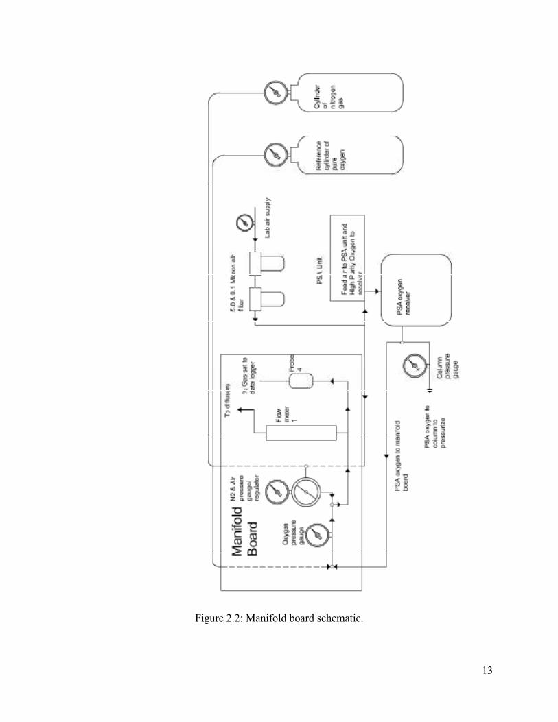
2.1.2 Air and Oxygen Flow Measurement

Air and oxygen gases were delivered through a custom built manifold board manufactured by

Point Four Systems, Inc. The manifold board was the same used in Ashley's (2002) research,

modified slightly. The manifold board was fitted with a Brooks Sho-Rate coarse scale flow meter

with a 150 mm scale, 2 to 12 L/min. The flow indicator was designed to operate at 45 psig (310

kPa), therefore a pressure regulator was also fitted to the manifold board. During

experimentation, the regulator for the different gases was set to 45 psig (310 kPa) prior to

entering the flow meter.

The flow meters were designed to read pure oxygen, therefore a specific density correction factor

(i.e. 1.105/1.0) was applied to the experiments that ran on compressed air (Ashley 2002). The

flow measurements were corrected to standard temperature and pressure, STP, values (i.e. 0°C,

101.325 kPa)

A small portion of the inflowing gas was sent to a cup constructed of a PVC pipe cap in which an

oxygen percent saturation probe (Probe 4) was connected. This probe measured the oxygen

purity of the inflowing gas to the diffusers. The gas that was measured came from the line before

the flow meter, so as to not affect the flow measurement. A reference cylinder of oxygen

(99.99% purity) was used to calibrate the oxygen probes. The reference cylinder was connected

to a two-stage pressure regulator before being piped to the manifold board. A cylinder of pure

nitrogen was used to mix the water, and was also connected to a two-stage pressure regulator and

to the manifold board. A schematic showing the different hose connections on the manifold

board can be seen in Figure 2.2.

13

Figure 2.2: Manifold board schematic.

14

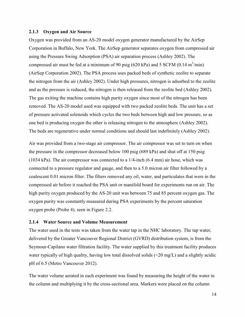
2.1.3 Oxygen and Air Source

Oxygen was provided from an AS-20 model oxygen generator manufactured by the AirSep

Corporation in Buffalo, New York. The AirSep generator separates oxygen from compressed air

using the Pressure Swing Adsorption (PSA) air separation process (Ashley 2002). The

compressed air must be fed at a minimum of 90 psig (620 kPa) and 5 SCFM (0.14 m3/min)

(AirSep Corporation 2002). The PSA process uses packed beds of synthetic zeolite to separate

the nitrogen from the air (Ashley 2002). Under high pressures, nitrogen is adsorbed to the zeolite

and as the pressure is reduced, the nitrogen is then released from the zeolite bed (Ashley 2002).

The gas exiting the machine contains high purity oxygen since most of the nitrogen has been

removed. The AS-20 model used was equipped with two packed zeolite beds. The unit has a set

of pressure activated solenoids which cycles the two beds between high and low pressure, so as

one bed is producing oxygen the other is releasing nitrogen to the atmosphere (Ashley 2002).

The beds are regenerative under normal conditions and should last indefinitely (Ashley 2002).

Air was provided from a two-stage air compressor. The air compressor was set to turn on when

the pressure in the compressor decreased below 100 psig (689 kPa) and shut off at 150 psig

(1034 kPa). The air compressor was connected to a 1/4-inch (6.4 mm) air hose, which was

connected to a pressure regulator and gauge, and then to a 5.0 micron air filter followed by a

coalescent 0.01 micron filter. The filters removed any oil, water, and particulates that were in the

compressed air before it reached the PSA unit or manifold board for experiments run on air. The

high purity oxygen produced by the AS-20 unit was between 75 and 85 percent oxygen gas. The

oxygen purity was constantly measured during PSA experiments by the percent saturation

oxygen probe (Probe 4), seen in Figure 2.2.

2.1.4 Water Source and Volume Measurement

The water used in the tests was taken from the water tap in the NHC laboratory. The tap water,

delivered by the Greater Vancouver Regional District (GVRD) distribution system, is from the

Seymour-Capilano water filtration facility. The water supplied by this treatment facility produces

water typically of high quality, having low total dissolved solids (<20 mg/L) and a slightly acidic

pH of 6.5 (Metro Vancouver 2012).

The water volume aerated in each experiment was found by measuring the height of the water in

the column and multiplying it by the cross-sectional area. Markers were placed on the column

15

every foot (30.5 cm) and a tape measure was used to measure the distance between the water

surface and the nearest marker. The water volume during experiments ranged between 235-245

L. The displacement caused by the probes and pumps was found to account for approximately

2.5 L; thus, this volume was subtracted from the volume calculated by measuring the water

height.

2.1.5 D.O. Probes

Specialty dissolved oxygen probes were purchased from Pentair Aquatic Eco-systems (formerly

Point Four Systems, Inc) in Coquitlam B.C. The high range stationary probes provided were the

OxyGuard Standard Type polarographic dissolved oxygen probe. In order to measure the high

levels of oxygen expected in the aeration column, the probes were modified to a configuration

slightly different from typical dissolved oxygen polarographic probes. The high range probe has

a smaller cathode than the conventional D.O. probe OxyGuard manufactures (Pentair Aquatic

Ecosystems 2013) . The oxygen polarographic probe is a galvanic sensor that produces a

millivolt (mV) signal directly proportional to the oxygen present in the medium the probe is

placed (Pentair Aquatic Ecosystems 2013). The probe consists of a cathode, anode, and a cap

that is fitted with a membrane and filled with electrolyte. Oxygen diffuses through the membrane

onto the cathode, where it reacts chemically, and then combines with the anode (OxyGuard

2013). This chemical process develops an electrical current which is converted to a mV output

signal through a resistor in the probe (OxyGuard 2013).

The probe has built in temperature compensation; therefore, no additional allowance is required

(Pentair Aquatic Ecosystems 2013). However, for this study probes were allowed to stabilize for

a minimum of ten minutes at the temperature of the medium they were placed. The OxyGuard

probes are designed for use between 0 and 40 degrees Celsius and a depth up to 100 meters

(OxyGuard 2013). Neither of these limits were exceeded in the experiments.

The oxygen probe measuring the percent oxygen in the inflowing gas (Probe 4) was fitted with a

"% saturation" membrane; while a "mg/L" membrane was fitted on D.O. probes 1-3 in the

column as per Pentair's instruction. The different probe membranes were required for accurate

measurement of either "mg/L" or "% saturation" for the respective probes. Probes 1-3 in the

column initially began collecting bubbles on the membranes during aeration; this led to probe

measurement of the oxygen content in the bubble, rather than the water. To solve this issue the

16

probes were attached to a 5-inch (12.7 cm) "L" bracket, tilting the probes at a 45° angle. This

allowed for bubbles to deflect off the membrane and continue rising in the column, ensuring

measurement of the dissolved oxygen in the water. This was confirmed during chemical

deoxygenation of the water (Section 2.3.1.1); in which the rate of decline in D.O. exuded by the

probes from nitrogen sparging would drastically increase, once sodium sulfite was added to the

column and began rapidly consuming the D.O in the water.

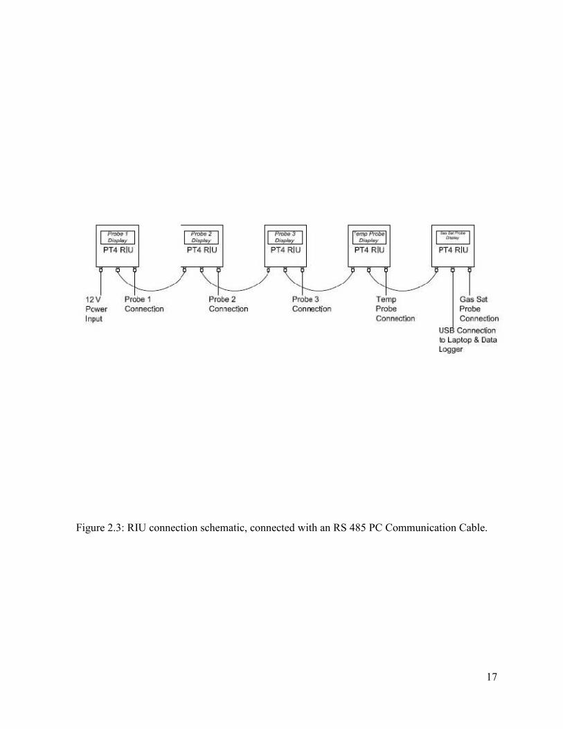
2.1.6 Data Logger

The D.O. probes were connected to their own respective PT4 Remote Interface Unit (RIU). The

PT4 RIU is a field mounted single sensor transmitter/controller. The unit will accept inputs from

any sensor providing a voltage, e.g. the D.O. probes. The PT4 RIU's were connected in series to

each other via an RS485 PC communication cable which was then connected to a Samsung

laptop via a USB cable. A schematic of the RIU setup is shown in Figure 2.3. The laptop was

installed with the PT4 Sync HMI Software system provided by Pentair. This software allowed

for user control of the data logger as well as a real-time view of the probe concentrations. Once

the data logging file was set, the system would record the 3 D.O. probe concentrations located in

the column, the temperature probe, and the percent oxygen probe (Probe 4). Concentrations for

these five probes were recorded every 10 seconds by the data logger in a .CSV file. Once an

experiment was finished, the data logger was stopped and the .CSV file was saved into an Excel

file name (.XLSX). The ASCE standard for reaeration states that, when a minimum number of

21 samples of D.O. measurements are obtained, the samples can be approximately equally

spaced from each other over the entire D.O. collection range. In each test, conducted for at least

45 minutes, at least 270 D.O. sample measurements were collected from the in situ probes, thus

satisfying the ASCE requirement. The actual manifold board and RIU configuration used in this

research are shown in Figure 2.4.

17

Figure 2.3: RIU connection schematic, connected with an RS 485 PC Communication Cable.

18

Figure 2.4: Manifold board and RIU configuration.

19

2.2 Experimental Design

2.2.1 Experimental Groups - Superoxygenation

This research aimed to find oxygen transfer rates and saturation concentrations in clean water at

different pressures, using high purity oxygen and air as the source of oxygen. Obtaining the same

data for air provided a base sample for comparative purposes between PSA and standard

aeration. The experimental groups were designed to increase in pressure incrementally by 50 kPa

(0.5 atmospheres), up to a pressure of 200 kPa (2 atmospheres). It was desired to record

measurements beyond this pressure; however, the reliability of the probes and structural integrity

of the column were of concern. The American Society of Civil Engineers (ASCE) standard for

oxygen transfer measurements requires a minimum of 3 replicates to be conducted for non-

steady state reaeration tests (ASCE 2007). Conducting experiments with 4 replicates was

selected for additional quality control. The data was analyzed by each probe individually, i.e. 4

replicates per probe, as well as by examining the column as a completely mixed reactor. This

allowed for the 3 probes to be used as duplicates for each experiment with 4 replicates, totaling

in 12 replicate samples to obtain an overall mean value for the reactor at each pressure.

The experimental groups conducted for the superoxygenation phase of the research are depicted

in Table 2.1.

Table 2.1: Superoxygenation experimental design

Gauge Pressure -

kPa (Atmospheres) Gas Type

Gas Flow Rate

(LPM)

No.

Experiments Replicates Total

0 (0) Oxygen/Air 4 2 4 8

50 (0.5) Oxygen/Air 4 2 4 8

100 (1.0) Oxygen/Air 4 2 4 8

150 (1.5) Oxygen/Air 4 2 4 8

200 (2.0) Oxygen/Air 4 2 4 8

Total

40

2.2.2 Experimental Groups - Deoxygenation

The research objectives also aimed to study the accompanying effervescence when the column

was depressurized with high D.O. concentrations, causing supersaturation. Therefore, at the

completion of each oxygenation experiment, a deoxygenation experiment began. In order to

determine the "spontaneity" of effervescence, the column was exposed to four different

20

environments (A-D) after superoxygenation, since the oxygenation phase had four replicates that

could be tested for effervescence.

A.) Depressurize to atmospheric pressure with the mixing pump active;

B.) Depressurize to atmospheric pressure without the mixing pump;

C.) Depressurize to 50 kPa (0.5 atmospheres) with the mixing pump active;

D.) Depressurize to 50 kPa (0.5 atmospheres) without the mixing pump active.

Conducting the research in this manner allowed for the validity of the assumption that

effervescence at more than 100% saturation is spontaneous to be determined. Finding the amount

of oxygen lost in each of the above four environments, if different from each other, would show

that other forces are needed for complete effervescence of water. Since there were four

depressurizing environments tested, only 1 replicate could be conducted. However, the data was

analyzed as a completely mixed reactor where the average effervescent loss was the average of

the 3 probes for each environment.

The experimental groups conducted for the deoxygenation phase of the research are depicted in

Table 2.2.

Table 2.2: Effervescence experimental design

Gauge Pressure -

kPa (Atmospheres) Gas Type Environment

No.

Experiments Replicates Total

50 (0.5) Oxygen/Air AB 4 2 8

100 (1.0) Oxygen/Air ABCD 8 1 8



Total 32

21

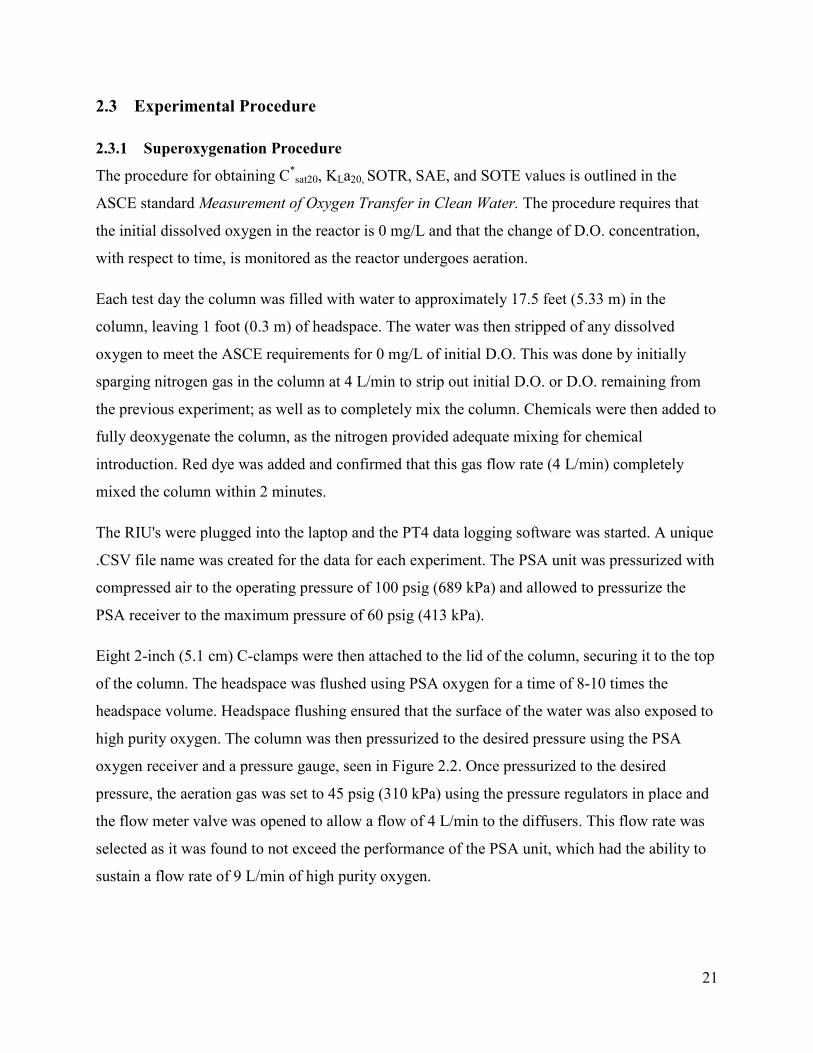
2.3 Experimental Procedure

2.3.1 Superoxygenation Procedure

The procedure for obtaining C*sat20, KLa20, SOTR, SAE, and SOTE values is outlined in the

ASCE standard Measurement of Oxygen Transfer in Clean Water. The procedure requires that

the initial dissolved oxygen in the reactor is 0 mg/L and that the change of D.O. concentration,

with respect to time, is monitored as the reactor undergoes aeration.

Each test day the column was filled with water to approximately 17.5 feet (5.33 m) in the

column, leaving 1 foot (0.3 m) of headspace. The water was then stripped of any dissolved

oxygen to meet the ASCE requirements for 0 mg/L of initial D.O. This was done by initially

sparging nitrogen gas in the column at 4 L/min to strip out initial D.O. or D.O. remaining from

the previous experiment; as well as to completely mix the column. Chemicals were then added to

fully deoxygenate the column, as the nitrogen provided adequate mixing for chemical

introduction. Red dye was added and confirmed that this gas flow rate (4 L/min) completely

mixed the column within 2 minutes.

The RIU's were plugged into the laptop and the PT4 data logging software was started. A unique

.CSV file name was created for the data for each experiment. The PSA unit was pressurized with

compressed air to the operating pressure of 100 psig (689 kPa) and allowed to pressurize the

PSA receiver to the maximum pressure of 60 psig (413 kPa).

Eight 2-inch (5.1 cm) C-clamps were then attached to the lid of the column, securing it to the top

of the column. The headspace was flushed using PSA oxygen for a time of 8-10 times the

headspace volume. Headspace flushing ensured that the surface of the water was also exposed to

high purity oxygen. The column was then pressurized to the desired pressure using the PSA

oxygen receiver and a pressure gauge, seen in Figure 2.2. Once pressurized to the desired

pressure, the aeration gas was set to 45 psig (310 kPa) using the pressure regulators in place and

the flow meter valve was opened to allow a flow of 4 L/min to the diffusers. This flow rate was

selected as it was found to not exceed the performance of the PSA unit, which had the ability to

sustain a flow rate of 9 L/min of high purity oxygen.

22

2.3.1.1 Chemical Deoxygenation Procedure

As per the ASCE, non-steady state reaeration procedure, the water needed to be stripped of any

dissolved oxygen prior to each experiment. This was partially done with the nitrogen sparging

which initiated a completely mixed regime, the remainder was removed by chemical oxidation.

The test water was deoxygenated with 0.1 mg/L of cobalt chloride as a catalyst and 7.9 mg/L of

sodium sulfite per mg/L of dissolved oxygen in the water (ASCE 2007). However, due to

oxidation during mixing it can be required to add up to 1.5 times the calculated amount of

sodium sulfite required for deoxygenation (Beak Consultants Ltd 1977). The cobalt chloride was

dissolved in a 500 mL bottle and added to the column and allowed to mix for a few minutes in

the column, by nitrogen sparging. The average D.O. concentration measured by probes 1-3 in the

column was used to determine the amount of sodium sulfite required for chemical

deoxygenation, applying a safety factor of 1.5. The amount of sodium sulfite required was

dissolved into a 1 liter flask and then added to the column to consume the remaining D.O.

Chemical deoxygenation limits the number of experiments that can be conducted on the same

test water to 5-8 experiments, as the solids concentration begins to accumulate and affect oxygen

transfer performance (ASCE 2007). It has been found that total dissolved solids (TDS)

concentrations below 2000 mg/L will not adversely affect oxygen transfer (ASCE 2007). The

number of experiments conducted on each test water was limited to 4. The largest amount of

sodium sulfite added to any one test water was 218 g (1.5 Pressure replicates - PSA) resulting in

a TDS concentration of 910 mg/L. Replicates were conducted in a random sequence so that

replicate 'D' (i.e., the fourth experiment) was not always completed fourth and, thus, always

exposed to higher TDS concentrations.

2.3.1.2 Probe Calibration

Calibration of the OxyGuard probes was completed as outlined in the OxyGuard manual and was

completed at the beginning of each day of experimentation. The probes were considered zero

stable, therefore a single point calibration would suffice (Pentair Aquatic Ecosystems 2013). Due

to the high concentrations the probes were measuring, it was impossible to reliably calibrate the

probes in water; therefore, Probes 1-4 were calibrated with the reference cylinder of pure

oxygen. Placing the probe in a pressure vessel would allow the probes to be calibrated to a higher

23

concentration, as it is desirable to calibrate as close as possible to a known value in the range at

which the probe will operate (Pentair Aquatic Ecosystems 2013).

Table 14, "Oxygen - mmHg per mg/L as a function of temperature", found in the Pentair manual

depicts the partial pressure of oxygen and the corresponding mg/L concentration as a function of

temperature. The absolute pressure that the probe was exposed to in pure oxygen could then be

converted to a known mg/L value for calibration. Probes 1-3 were calibrated daily before each

experiment and were calibrated at the pressure that was going to be tested in the column for that

round of experiments. The probes were attached to a PVC cap via hose clamps to secure the

probe in the cap. Pure oxygen was then used to pressurize the cap and probe to the desired

pressure for calibration. The calibrating mg/L concentration was then set on the RIU's. Figure 2.5

shows the probe in the pressure vessel used for calibration. The percent saturation probe was

calibrated at atmospheric pressure using the reference cylinder of pure oxygen.

24

Figure 2.5: Probe attached to calibration vessel.

The temperature probe was calibrated to room temperature using a thermometer. The

temperature probe was checked daily, checking the measured temperature of the water from the

probe and from the thermometer, where no significant difference was ever found. The data

logger recorded the temperature in the water every 10 seconds and the average temperature for

the duration of aeration was used for the parameter estimations. The temperature of an

25

experiment did not vary by more than 1°C, for any superoxygenation or effervescence

experiment.

2.3.1.3 Termination of Experiments

The method of parameter estimation, as will be outlined in Section 2.4, requires that aeration

during an experiment occurs for a time "no less than 4/KLa20" (ASCE 2007). Initial experiments

concluded that aeration of 45 minutes would suffice in the water reaching 99% saturation and an

accurate estimation of the parameters desired.

2.3.2 Effervescence Deoxygenation Procedure

The effervescing deoxygenation procedure was done to monitor the effects of water saturated at

a given pressure being rapidly exposed to atmospheric conditions, thus supersaturating the water

causing effervescence. For environments A and C (pump on) the pump was turned on prior to

depressurizing the column. The column was then depressurized to either gauge pressures of 0 or

50 kPa, depending on which environment was tested. The column was then allowed to effervesce

for 20 minutes. Initial experiments found that most dissolved oxygen was lost in the first 5

minutes of effervescence when the concentration in the water was highest. The difference in

effervescence between 20 and 30 minutes was not significant and, thus, did not justify

monitoring for a time longer than 20 minutes, while staying within reason. It was also found that

experiments conducted on a Friday would still have water at or above saturation values the

following Monday; indicating that effervescence seemingly follows an inverse exponential

curve.

Experiments conducted on effervescence found that the effervescing bubbles in the water were

very small, lacking high rise velocities. The effervescing bubbles would stick to the D.O. probes'

membrane, even with the probes tilted at 45°, causing the D.O. probes to read the concentration

of oxygen in the bubbles rather than the water. Therefore, once the water was allowed to

effervesce for 20 minutes, the water column was sparged with nitrogen gas at 6 L/min to remove

the fine bubbles trapped on the probes. The nitrogen gas bubbles freed the finer oxygen bubbles

within 30 seconds and the probes began accurately measuring the concentration of D.O. in the

water. Sparging occurred until the concentration the probes measured began to decrease;

indicating that nitrogen gas had begun stripping out oxygen from the water (about 3 minutes).

This allowed for an initial and final concentration to be measured over the 20 minute

26

effervescing span, resulting in a percent loss of oxygen for each probe. When measuring high

concentrations of D.O. in the water it was expected that the amount of oxygen removed by

nitrogen sparging in the 3 minute time frame (< 5 mg/L) would be very minimal in comparison.

Additionally, the values of percent D.O. loss would give conservative estimates for

effervescence, as they included the minimal amounts lost from the short time of nitrogen

sparging.

There is no written standard for effervescence testing; therefore, all assumptions such as

environments A-D, effervescence time, and the use of nitrogen sparging were derived from

observation during preliminary experiments. The effervescence procedure was developed with

the intent of showcasing the effects different factors have on the amount of D.O. loss to

effervescence.

2.4 Parameter Estimation

Oxygen transfer is modeled through the exponential equation according to Equation 2.1 (Brown

and Baillod 1982):

= ∗ − ∗ − ∗ ( 2.1 )

where:

= The dissolved oxygen concentration in the test water at temperature T and time t;

∗ = The dissolved oxygen saturation value (mg/L) for the ambient barometric pressure and

temperature T of the test water;

= Initial dissolved oxygen concentration at test temperature T (mg/L);

= Oxygen overall mass transfer coefficient at the temperature T of the test water (hr-1

);

t = Time at which the value of C is desired (hr).

Typically, KLaT is the only unknown value of Equation 2.1. C*sat can be assumed using air-

saturation values for varying temperatures and barometric pressures in academic tables (log-

deficit method). C0 can be assumed to be 0 mg/L since the reaeration test requires 0 mg/L of

initial dissolved oxygen in the test water, leaving KLaT as the only unknown. Monitoring the

27

change in the dissolved oxygen profile, with respect to time, will solve Equation 2.1. However,

using high purity oxygen and higher pressures to attain unknown saturation values adds an extra

variable to the equation, as C*sat becomes an unknown. Thus, the non-linear regression method,

as is the preferred method by the ASCE standard, was employed to solve Equation 2.1.

The method is based on non-linear regression of Equation 2.1 through the D.O.-versus-time data

that is logged in each experiment. The best estimates for the variables (C*sat, KLaT) are selected

as "the values that drive the model equation through the prepared D.O. concentration-versus-time

data points with a minimum residual sum of squares" (ASCE 2007). The residual is the

difference in concentration between a measured D.O. value at a given time and a D.O. value that

is predicted by the model at the same time step (ASCE 2007). Application of this method to

solve one equation with two unknowns requires the assistance of computer software. A

spreadsheet was supplied with the ASCE standard, coded by Michael Stenstrom, primary author

of the ASCE reaeration standard. The spreadsheet allows for user input of the D.O.

concentration-versus-time data and outputs values for C*sat and KLaT. Additionally, the program

will output the residual sum of squares for the parameter values generated. A sample of the

spreadsheet with D.O. data from this research can be seen in Appendix 1.

The KLa found for each experiment had to then be corrected to 20°C, if the experiment was not

conducted at that temperature. KLaT was converted to KLa20 according to Equation 2.2:

= ( 2.2 )

where:

= Oxygen transfer coefficient at 20°C (hr-1

);

= Oxygen transfer coefficient at test temperature T (hr-1

);

θ = 1.024 (Tchobanoglous et al. 2003);

T = Water test temperature.

Similarly to KLa, C*sat at the test temperature needed to be converted to standard conditions of

20°C. Since C*sat is also dependent on the barometric pressure the saturation concentration

28

needed to be corrected to a standard pressure of 101.325 kPa. This was done according to

Equation 2.3:

∗ = ∗ ! "#$% ( 2.3 )

where:

∗ = Oxygen saturation concentration at 20°C and 101.325 kPa barometric pressure (mg/L);

∗ = Oxygen saturation concentration at test temperature and test barometric pressure (mg/L);

τ = Temperature correction factor =

&'()*+',-./0./1)/,-./))23),',)/*&,.2),-13,)',) &'()*+',-./0./1)/,-./*)4,))/*"".56789.:24/ ;

Ω = Pressure correction factor = ;,.2),-18,)',)+-)

+/*,*8,)',)"".5678.

It is important to note that tabulated concentration values, for the temperature correction factor,

were obtained from tables containing the data for the air-water saturation concentration

relationship. This same temperature correction factor was assumed to apply to saturation

concentrations gathered throughout the data collection, even at the high concentrations obtained

at high pressures. Experiments, however, were conducted as close to 20°C as possible (15-21

degrees) for PSA oxygen to minimize potential error from the temperature correction factor.

Experiments conducted on air ranged from 10-20 degrees Celsius; however, the temperature

correction factor was assumed to cause less error when used with air.

The SOTR was calculated according to Equation 2.4:

<=>? = ∗ @ ( 2.4 )

where:

SOTR = Standard oxygen transfer rate (g O2/hr);

= Oxygen transfer coefficient at 20°C (hr-1

);

∗ = Oxygen saturation concentration at 20°C and 101.325 kPa (mg/L);

29

V = Volume of water in the column (m3).

SOTE was calculated as (Equation 2.5):

<=>A = +B CDEF

( 2.5 )

where:

SOTE = Standard oxygen transfer efficiency (%);


WO2 = Mass flow rate of oxygen in the gas flow stream (g O2/hr).

For experiments conducted with air, WO2 was calculated as the measured gas flow, corrected to

standard conditions, multiplied by the weight of oxygen in air (0.3 g/L at STP) and converted to

g O2/hr (Ashley 2002). This can be found in Equation 2.6.

GB-,H = ℎJ⁄ = HLMNOPQ min⁄ ∗ 0.3H = Q⁄ ∗ 60WXY ℎJ⁄ ( 2.6 )

For experiments conducted with PSA oxygen, WO2 was calculated as the sum of the measured

gas flow, corrected to standard conditions, multiplied by the percent of oxygen in the gas and the

weight of pure oxygen (1.4277 g/L at STP) (Ashley 2002). The percent of oxygen in the gas was

taken as the average reading of Probe 4 throughout the experiment (75-85%). This calculation is

shown in Equation 2.7.

GB8+H= ℎJ⁄ = HLMNOPQ min⁄ ∗ %= ∗ 1.4277H = Q⁄ ∗ 60WXY ℎJ⁄ ( 2.7 )

The SAE was calculated as (Equation 2.8):

<^A = +B C8._),`/3' ( 2.8 )

where:

SAE = Standard aeration efficiency (g O2/kWhr);


Power Input = Total delivered power (kW).

30

The calculation of the delivered power to each experiment is outlined in the next section (2.4.1).

2.4.1 Power Estimation

The power was estimated from adiabatic compression of a gas to a given discharge pressure.

This is the theoretical power required at blower discharge to deliver a given mass flow of gas at a

given discharge pressure (ASCE 2007). The delivered blower power, calculated according to the

adiabatic compression formula, can be found in Equation 2.9. The power equation and

calculations used were the same as outlined by Ashley (2002).

a_ = _C b9.:/) [ "⁄ / − 1] ( 2.9 )

where:

Pw = Power input (kW);

w = Weight of air flow (kg/s) (i.e., 1.2927 g/L);

R = Engineering gas constant, 8.314 kJ/k mol °K;

T1 = Absolute inlet temperature before compression (°K);

p1 = Absolute inlet pressure before compression (i.e., 101.325 kPa);

p2 = Absolute inlet pressure after compression;

k = Ratio of specific heats for gas = 1.395 for air and oxygen;

n = (k-1)/k = 0.283 for air and oxygen;

29.7 = Constant for SI conversion;

e = Compressor efficiency, 0.80 (ASCE 2007; Ashley 2002).

On air, the adiabatic compression was separated into two components, Pw1 and Pw2. Pw1 was

calculated using the absolute delivery pressure from the manifold board regulator, i.e. 60 psia

(413 kPa). Pw2 is the same adiabatic compression formula adjusted for the absolute ambient

hydrostatic pressure of the diffusers plus the total column pressure as the inlet pressure after

compression (p2). The sum of the two power components equals the total delivered power.

31

For experiments on PSA oxygen, the power input was separated into three components plus an

expansion factor for the weight of air flow (w; kg/s), based on the published air input to oxygen

output ratio of the AS-20 PSA unit (i.e., 15.9:1) (AirSep Corporation 2002; Ashley 2002). The

first component, Pw1, is the delivered blower power required to deliver the mass flow of gas at

the absolute minimum pressure requirement of the PSA unit, i.e. 105 psia (723 kPa) (Ashley

2002). Similarly to Pw2 for air, Pw2 for PSA is the same adiabatic compression formula adjusted

to the absolute ambient hydrostatic pressure plus the total column pressure on the diffusers.

Finally, the third component, Pw3, is the average measured wire power of the AS-20 unit. Wire

power was calculated according to:

a = e ∗ @ ( 2.10 )

where:

P = Wire power (Watts);

I = Measured current (amps);

V = Measured potential (Volts) (Kowsari 2008).

The average measured wire power of the PSA unit was 0.02938 kW. Voltage and current were

measured in the PSA unit during several oxygen cycles to obtain average values for power

calculation. The sum of the three power components is the total delivered power for PSA

oxygen. Voltage and current were measured with a Fluke multi-meter. Table 2.3 summarizes the

power components and calculations for air and PSA oxygen.

Table 2.3: Power calculations for superoxygenation treatments.

Treatment Pw1 Pw2 Pw3

Air

Adiabatic

compression

@ 60 psia

(413 kPa)

Adiabatic compression @ x m

depth + column absolute pressure

(i.e. 100, 150, 200, 250, 300 kPa)

n/a

PSA

Adiabatic

compression

@ 105 psia

(723 kPa)

Adiabatic compression @ x m

depth + column absolute pressure

(i.e. 100, 150, 200, 250, 300 kPa)

Average measured

wire power to PSA

unit (i.e. 0.02938 kW)

32

2.5 Statistical Analysis

To account for lingering effects from excess sodium sulfite added in the chemical deoxygenation

procedure, low-end data truncation was applied to the D.O. concentration-versus-time raw data.

ASCE recommends that data below 20% of C*sat be removed from the data series, if there is an

apparent interaction with excess sodium sulfite (ASCE 2007). This was applied in all

experiments conducted for consistency and to negate any adverse effects from excess sodium

sulfite.

The mean values for KLa20, C*sat20, SOTR, SOTE, and SAE were determined, along with the

standard deviations and standard errors for each. ASCE requires a standard for the repeatability

of replicate samples measured. This standard requires that when a series of at least three replicate

tests are conducted, the KLa20 values must not vary by more than ± 15% from the mean for the

values for that probe (ASCE 2007). Values that are outside of the range will be considered as

invalid and not used in any further calculations. However, since the experiments were outside

pressures and saturation concentrations for which the ASCE standard was established, the data

was analyzed without KLa20 values that were outside the range specified and with said KLa20

values included. Since four replicates were conducted at each pressure, the removal of any value

outside of the 15% range still resulted in three replicates that could be used in all experiments

and for all probes.

Additionally, a total mean value was obtained viewing the column as a completely mixed

reactor, exposed to the total headspace pressure and one-half of the water column depth as

additional hydrostatic pressure. Using the three probes as duplicates in this manner allowed for

12 data points to be obtained (4 replicates x 3 probes) for finding an overall mean for the desired

parameters. This average was also analyzed using the 15% range requirement of ASCE for KLa20

values, still resulting in at least 9 data points to be used at all pressures for a mean value of each

parameter.

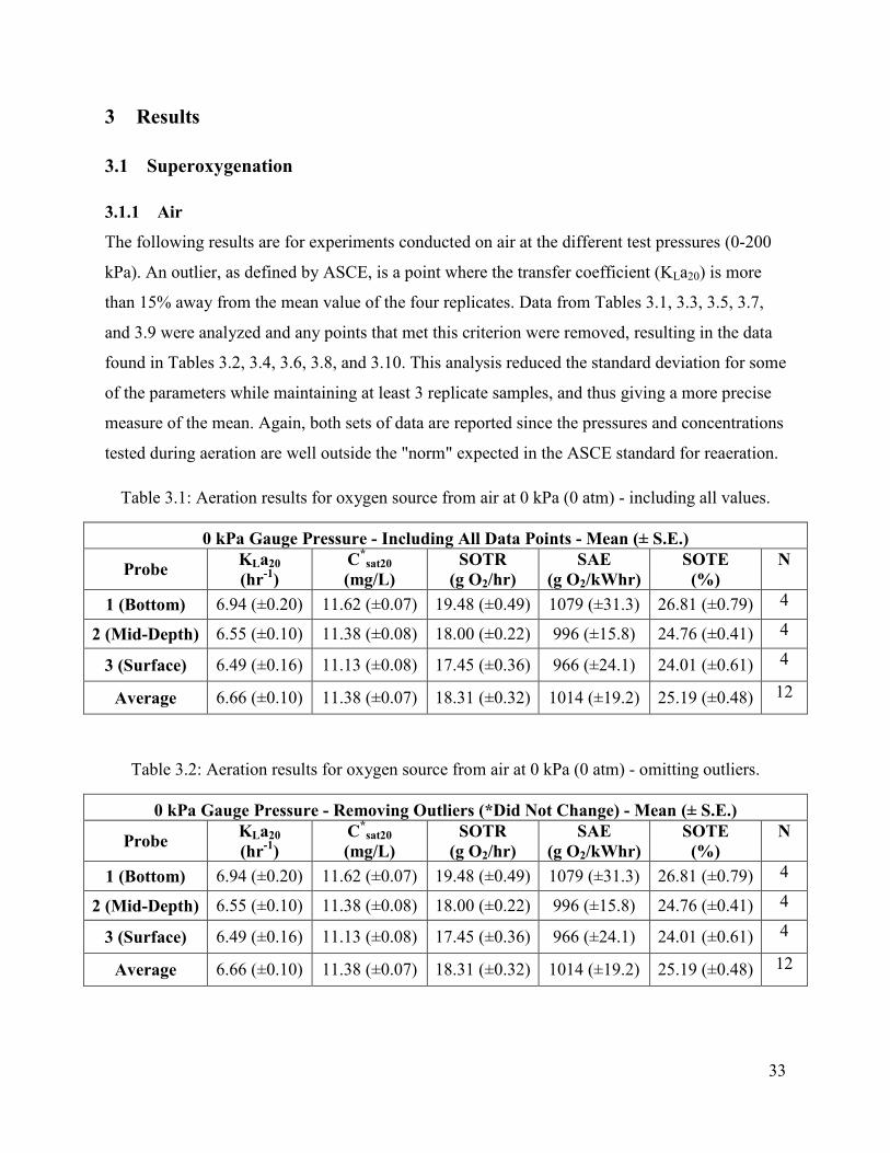
33

3 Results

3.1 Superoxygenation

3.1.1 Air

The following results are for experiments conducted on air at the different test pressures (0-200

kPa). An outlier, as defined by ASCE, is a point where the transfer coefficient (KLa20) is more

than 15% away from the mean value of the four replicates. Data from Tables 3.1, 3.3, 3.5, 3.7,

and 3.9 were analyzed and any points that met this criterion were removed, resulting in the data

found in Tables 3.2, 3.4, 3.6, 3.8, and 3.10. This analysis reduced the standard deviation for some

of the parameters while maintaining at least 3 replicate samples, and thus giving a more precise

measure of the mean. Again, both sets of data are reported since the pressures and concentrations

tested during aeration are well outside the "norm" expected in the ASCE standard for reaeration.

Table 3.1: Aeration results for oxygen source from air at 0 kPa (0 atm) - including all values.

0 kPa Gauge Pressure - Including All Data Points - Mean (± S.E.)

Probe KLa20

(hr-1

)

C*

sat20

(mg/L)

SOTR

(g O2/hr)

SAE

(g O2/kWhr)

SOTE

(%)

N

1 (Bottom) 6.94 (±0.20) 11.62 (±0.07) 19.48 (±0.49) 1079 (±31.3) 26.81 (±0.79) 4

2 (Mid-Depth) 6.55 (±0.10) 11.38 (±0.08) 18.00 (±0.22) 996 (±15.8) 24.76 (±0.41) 4

3 (Surface) 6.49 (±0.16) 11.13 (±0.08) 17.45 (±0.36) 966 (±24.1) 24.01 (±0.61) 4

Average 6.66 (±0.10) 11.38 (±0.07) 18.31 (±0.32) 1014 (±19.2) 25.19 (±0.48) 12

Table 3.2: Aeration results for oxygen source from air at 0 kPa (0 atm) - omitting outliers.

0 kPa Gauge Pressure - Removing Outliers (*Did Not Change) - Mean (± S.E.)

Probe KLa20

(hr-1

)

C*

sat20

(mg/L)

SOTR

(g O2/hr)

SAE

(g O2/kWhr)

SOTE

(%)

N

1 (Bottom) 6.94 (±0.20) 11.62 (±0.07) 19.48 (±0.49) 1079 (±31.3) 26.81 (±0.79) 4

2 (Mid-Depth) 6.55 (±0.10) 11.38 (±0.08) 18.00 (±0.22) 996 (±15.8) 24.76 (±0.41) 4

3 (Surface) 6.49 (±0.16) 11.13 (±0.08) 17.45 (±0.36) 966 (±24.1) 24.01 (±0.61) 4

Average 6.66 (±0.10) 11.38 (±0.07) 18.31 (±0.32) 1014 (±19.2) 25.19 (±0.48) 12

34



Probe KLa20

(hr-1

)

C*

sat20

(mg/L)

SOTR

(g O2/hr)

SAE

(g O2/kWhr)

SOTE

(%)

N

1 (Bottom) 4.84 (±0.41) 19.20 (±1.31) 22.11 (±1.76) 1078 (±86.8) 30.83 (±2.48) 4

2 (Mid-Depth) 5.42 (±0.29) 16.82 (±0.36) 22.01 (±1.56) 1073 (±76.3) 30.68 (±2.18) 4

3 (Surface) 4.92 (±0.43) 16.17 (±0.63) 19.36 (±2.35) 943 (±111) 26.95 (±3.17) 4

Average 5.06 (±0.21) 17.39 (±0.60) 21.16 (±1.08) 1031 (±51.8) 29.49 (±1.48) 12


50 kPa Gauge Pressure - Removing Outliers ('*' Indicates Change) - Mean (± S.E.)

Probe KLa20

(hr-1

)

C*

sat20

(mg/L)

SOTR

(g O2/hr)

SAE

(g O2/kWhr)

SOTE

(%)

N

1 (Bottom)* 5.25 (±0.04) 18.38 (±1.45) 23.22 (±1.94) 1130 (±98.3) 32.31 (±2.80) 3

2 (Mid-Depth) 5.42 (±0.29) 16.82 (±0.36) 22.01 (±1.56) 1073 (±76.3) 30.68 (±2.18) 4

3 (Surface) 4.92 (±0.43) 16.17 (±0.63) 19.36 (±2.35) 943 (±111) 26.95 (±3.17) 4

Average* 5.10 (±0.18) 17.01 (±0.50) 21.37 (±1.15) 1041 (±55.7) 29.77 (±1.59) 11

35



Probe KLa20

(hr-1

)

C*

sat20

(mg/L)

SOTR

(g O2/hr)

SAE

(g O2/kWhr)

SOTE

(%)

N

1 (Bottom) 4.39 (±0.30) 24.06 (±1.97) 25.25 (±1.89) 1122 (±82.3) 35.61 (±2.61) 4

2 (Mid-Depth) 4.81 (±0.34) 21.20 (±0.32) 24.64 (±1.82) 1095 (±79.7) 34.75 (±2.52) 4

3 (Surface) 3.93 (±0.49) 19.49 (±1.09) 18.24 (±1.68) 811 (±75.8) 25.74 (±2.41) 4

Average 4.38 (±0.23) 21.58 (±0.89) 22.71 (±1.34) 1009 (±59.3) 32.03 (±1.88) 12



Probe KLa20

(hr-1

)

C*

sat20

(mg/L)

SOTR

(g O2/hr)

SAE

(g O2/kWhr)

SOTE

(%)

N

1 (Bottom) 4.39 (±0.30) 24.06 (±1.97) 25.25 (±1.89) 1122 (±82.3) 35.61 (±2.61) 4

2 (Mid-

Depth)* 5.14 (±0.09) 21.24 (±0.45) 26.33 (±0.91) 1170 (±38.2) 37.13 (±1.21)

3

3 (Surface)* 4.33 (±0.40) 19.06 (±1.42) 19.76 (±1.02) 879 (±45.7) 27.92 (±1.45) 3

Average* 4.60 (±0.19) 21.71 (±1.07) 23.93 (±1.21) 1063 (±52.9) 33.76 (±1.68) 10

36



Probe KLa20

(hr-1

)

C*

sat20

(mg/L)

SOTR

(g O2/hr)

SAE

(g O2/kWhr)

SOTE

(%)

N

1 (Bottom) 4.35 (±0.08) 30.36 (±0.72) 31.57 (±1.36) 1288 (±52.2) 44.37 (±1.80) 4

2 (Mid-Depth) 3.38 (±0.50) 31.43 (±2.42) 24.58 (±2.42) 1003 (±98.1) 34.55 (±3.38) 4

3 (Surface) 2.83 (±0.15) 28.71 (±1.44) 19.25 (±0.47) 786 (±17.1) 27.06 (±0.59) 4

Average 3.52 (±0.25) 30.17 (±0.94) 25.13 (±1.74) 1026 (±70.7) 35.33 (±2.44) 12



Probe KLa20

(hr-1

)

C*

sat20

(mg/L)

SOTR

(g O2/hr)

SAE

(g O2/kWhr)

SOTE

(%)

N

1 (Bottom) 4.35 (±0.08) 30.36 (±0.72) 31.57 (±1.36) 1288 (±52.2) 44.37 (±1.80) 4

2 (Mid-

Depth)* 3.84 (±0.27) 29.37 (±1.80) 26.80 (±1.33) 1093 (±56.0) 37.65 (±1.93)

3

3 (Surface) 2.83 (±0.15) 28.71 (±1.44) 19.25 (±0.47) 786 (±17.1) 27.06 (±0.59) 4

Average* 3.66 (±0.22) 29.49 (±0.71) 25.79 (±1.77) 1052 (±71.8) 36.24 (±2.47) 11

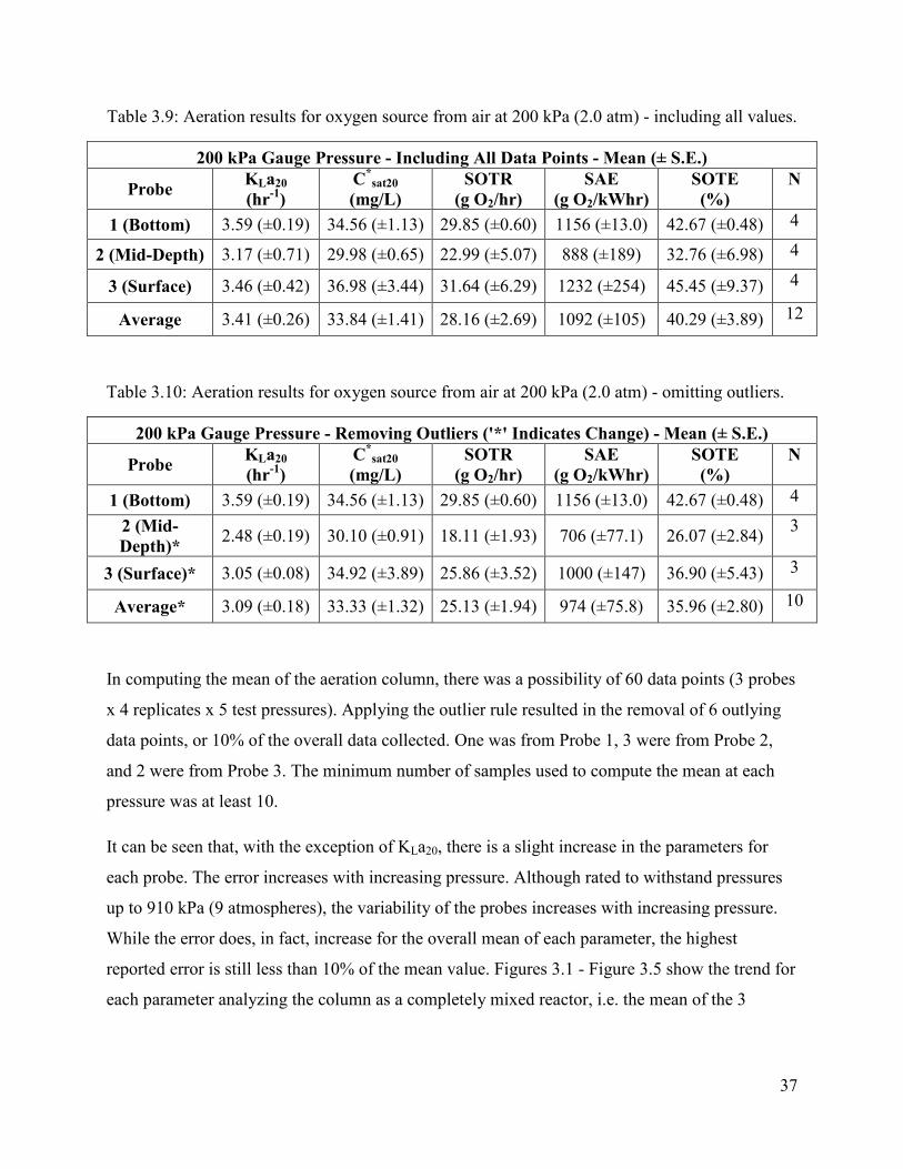
37



Probe KLa20

(hr-1

)

C*

sat20

(mg/L)

SOTR

(g O2/hr)

SAE

(g O2/kWhr)

SOTE

(%)

N

1 (Bottom) 3.59 (±0.19) 34.56 (±1.13) 29.85 (±0.60) 1156 (±13.0) 42.67 (±0.48) 4

2 (Mid-Depth) 3.17 (±0.71) 29.98 (±0.65) 22.99 (±5.07) 888 (±189) 32.76 (±6.98) 4

3 (Surface) 3.46 (±0.42) 36.98 (±3.44) 31.64 (±6.29) 1232 (±254) 45.45 (±9.37) 4

Average 3.41 (±0.26) 33.84 (±1.41) 28.16 (±2.69) 1092 (±105) 40.29 (±3.89) 12



Probe KLa20

(hr-1

)

C*

sat20

(mg/L)

SOTR

(g O2/hr)

SAE

(g O2/kWhr)

SOTE

(%)

N

1 (Bottom) 3.59 (±0.19) 34.56 (±1.13) 29.85 (±0.60) 1156 (±13.0) 42.67 (±0.48) 4

2 (Mid-

Depth)* 2.48 (±0.19) 30.10 (±0.91) 18.11 (±1.93) 706 (±77.1) 26.07 (±2.84)

3

3 (Surface)* 3.05 (±0.08) 34.92 (±3.89) 25.86 (±3.52) 1000 (±147) 36.90 (±5.43) 3

Average* 3.09 (±0.18) 33.33 (±1.32) 25.13 (±1.94) 974 (±75.8) 35.96 (±2.80) 10

In computing the mean of the aeration column, there was a possibility of 60 data points (3 probes

x 4 replicates x 5 test pressures). Applying the outlier rule resulted in the removal of 6 outlying

data points, or 10% of the overall data collected. One was from Probe 1, 3 were from Probe 2,

and 2 were from Probe 3. The minimum number of samples used to compute the mean at each

pressure was at least 10.

It can be seen that, with the exception of KLa20, there is a slight increase in the parameters for

each probe. The error increases with increasing pressure. Although rated to withstand pressures

up to 910 kPa (9 atmospheres), the variability of the probes increases with increasing pressure.

While the error does, in fact, increase for the overall mean of each parameter, the highest

reported error is still less than 10% of the mean value. Figures 3.1 - Figure 3.5 show the trend for

each parameter analyzing the column as a completely mixed reactor, i.e. the mean of the 3

38

probes at each pressure. The graphs plotted are for the data that excludes outliers and contain the

standard error for each data point.

Figure 3.1: Overall mass transfer coefficient for air.

The overall mass transfer coefficient (KLa20) steadily decreased with increasing pressure. KLa20

decreases approximately 0.5 fold over the range of pressures tested. Similar results were

obtained for PSA oxygen. A possible cause of reduced KLa20 values is that the higher pressure

causes smaller bubble size and thus a slower rise velocity of the bubbles. The decrease in rise

velocity causes a decrease in the turbulence in the water and the surface renewal rate of the

liquid film, affecting KLa20. This will be elaborated on further in the discussion.

0.00

1.00

2.00

3.00

4.00

5.00

6.00

7.00

8.00

0 50 100 150 200 250

KLa

20

(hr

-1)

Pressure (kPa)

Average Air Mass Transfer Coefficient, KLa20

39

Figure 3.2: Saturation concentration for air.

Figure 3.2 includes the concentration found from using Henry's law to estimate the saturation

concentration. This calculation was done using 21% oxygen in air and the total pressure in the

column plus one-half of the total water depth to estimate the partial pressure. The 20°C Henry's

constant used was 40,100 atmospheres/mole fraction (Nevers 2013). The 150 and 200 kPa

pressures (1.5 and 2.0 atmospheres, respectively) indicate that there may be some interaction

with Henry's constant and increasing pressure.

0.00

5.00

10.00

15.00

20.00

25.00

30.00

35.00

40.00

0 50 100 150 200 250

C*sa

t20

(mg

/L)

Pressure (kPa)

Average Air Saturation Concentration, C*sat20

Average C*

Henry's Law

40

Figure 3.3: Air standard oxygen transfer rate.

The oxygen transfer rate (SOTR) increased over the range of pressures tested, seen in Figure 3.3;

however, this increase is very minimal (~1.5 fold). The minimal change in SOTR is possibly due

to the ability of oxygen to transfer across the bubble film not changing dramatically with

pressure; thus, the oxygen transfer rate stays nearly constant. (Similar results were obtained in

the experiments conducted with PSA in that minimal changes in SOTR occurred).

0.00

5.00

10.00

15.00

20.00

25.00

30.00

0 50 100 150 200 250

SO

TR

(g

O2/h

r)

Pressure (kPa)

Average Air SOTR

41

Figure 3.4: Air standard aeration efficiency.

Figure 3.4 indicates that the aeration efficiency stayed nearly constant over the range of

pressures tested. The primary input for SAE calculation is SOTR, which was found to have a

minimal change. The other input to SAE calculation is the power required for aeration. The

theoretical power required at blower discharge did not change significantly over the range of

pressures tested for air.

0.00

200.00

400.00

600.00

800.00

1000.00

1200.00

0 50 100 150 200 250

SA

E (

g O

2/k

Wh

r)

Pressure (kPa)

Average Air SAE

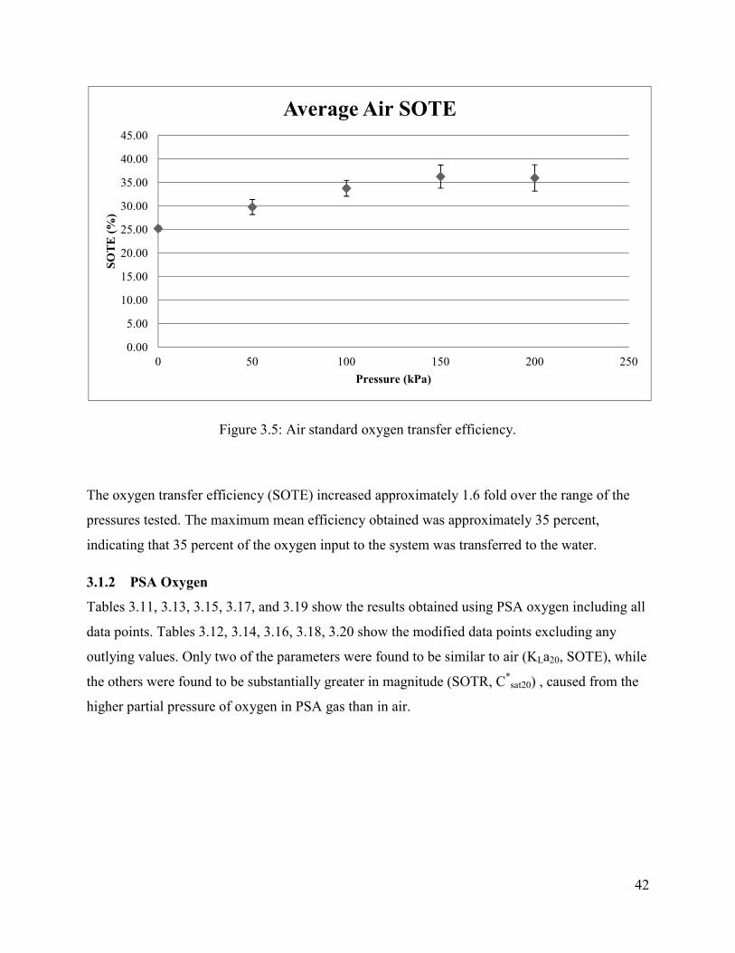
42

Figure 3.5: Air standard oxygen transfer efficiency.

The oxygen transfer efficiency (SOTE) increased approximately 1.6 fold over the range of the

pressures tested. The maximum mean efficiency obtained was approximately 35 percent,

indicating that 35 percent of the oxygen input to the system was transferred to the water.

3.1.2 PSA Oxygen

Tables 3.11, 3.13, 3.15, 3.17, and 3.19 show the results obtained using PSA oxygen including all

data points. Tables 3.12, 3.14, 3.16, 3.18, 3.20 show the modified data points excluding any

outlying values. Only two of the parameters were found to be similar to air (KLa20, SOTE), while

the others were found to be substantially greater in magnitude (SOTR, C*sat20) , caused from the

higher partial pressure of oxygen in PSA gas than in air.

0.00

5.00

10.00

15.00

20.00

25.00

30.00

35.00

40.00

45.00

0 50 100 150 200 250

SO

TE

(%

)

Pressure (kPa)

Average Air SOTE

43

Table 3.11: Aeration results for oxygen source from PSA at 0 kPa (0 atm) - including all values.


Probe KLa20

(hr-1

)

C*

sat20

(mg/L)

SOTR

(g O2/hr)

SAE

(g O2/kWhr)

SOTE

(%)

N

1 (Bottom) 7.85 (±0.50) 51.37 (±0.32) 97.75 (±6.76) 241.0 (±16.6) 35.12 (±2.45) 4

2 (Mid-Depth) 8.13 (±0.28) 49.63 (±0.42) 97.89 (±4.45) 241.3 (±10.9) 35.17 (±1.61) 4

3 (Surface) 8.27 (±0.30) 49.17 (±0.33) 98.62 (±4.42) 243.1 (±10.8) 35.43 (±1.60) 4

Average 8.08 (±0.20) 50.06 (±0.34) 98.09 (±2.78) 241.8 (±6.8) 35.24 (±1.00) 12

Table 3.12: Aeration results for oxygen source from PSA at 0 kPa (0 atm) - omitting outliers.


Probe KLa20

(hr-1

)

C*

sat20

(mg/L)

SOTR

(g O2/hr)

SAE

(g O2/kWhr)

SOTE

(%)

N

1 (Bottom)* 8.31 (±0.25) 51.60 (±0.32) 104.1 (±3.45) 256.4 (±8.4) 37.40 (±1.24) 3

2 (Mid-Depth) 8.13 (±0.28) 49.63 (±0.42) 97.89 (±4.45) 241.3 (±10.9) 35.17 (±1.61) 4

3 (Surface) 8.27 (±0.30) 49.17 (±0.33) 98.62 (±4.42) 243.1 (±10.8) 35.43 (±1.60) 4

Average* 8.23 (±0.15) 50.00 (±0.37) 98.84 (±2.37) 246.1 (±5.8) 35.87 (±0.86) 11

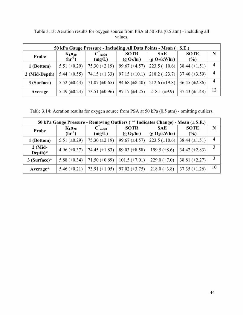
44


values.


Probe KLa20

(hr-1

)

C*

sat20

(mg/L)

SOTR

(g O2/hr)

SAE

(g O2/kWhr)

SOTE

(%)

N

1 (Bottom) 5.51 (±0.29) 75.30 (±2.19) 99.67 (±4.57) 223.5 (±10.6) 38.44 (±1.51) 4

2 (Mid-Depth) 5.44 (±0.55) 74.15 (±1.33) 97.15 (±10.1) 218.2 (±23.7) 37.40 (±3.59) 4

3 (Surface) 5.52 (±0.43) 71.07 (±0.65) 94.68 (±8.40) 212.6 (±19.8) 36.45 (±2.86) 4

Average 5.49 (±0.23) 73.51 (±0.96) 97.17 (±4.25) 218.1 (±9.9) 37.43 (±1.48) 12

Table 3.14: Aeration results for oxygen source from PSA at 50 kPa (0.5 atm) - omitting outliers.


Probe KLa20

(hr-1

)

C*

sat20

(mg/L)

SOTR

(g O2/hr)

SAE

(g O2/kWhr)

SOTE

(%)

N

1 (Bottom) 5.51 (±0.29) 75.30 (±2.19) 99.67 (±4.57) 223.5 (±10.6) 38.44 (±1.51) 4

2 (Mid-

Depth)* 4.96 (±0.37) 74.45 (±1.83) 89.03 (±8.58) 199.5 (±8.6) 34.42 (±2.83)

3

3 (Surface)* 5.88 (±0.34) 71.50 (±0.69) 101.5 (±7.01) 229.0 (±7.0) 38.81 (±2.27) 3

Average* 5.46 (±0.21) 73.91 (±1.05) 97.02 (±3.75) 218.0 (±3.8) 37.35 (±1.26) 10

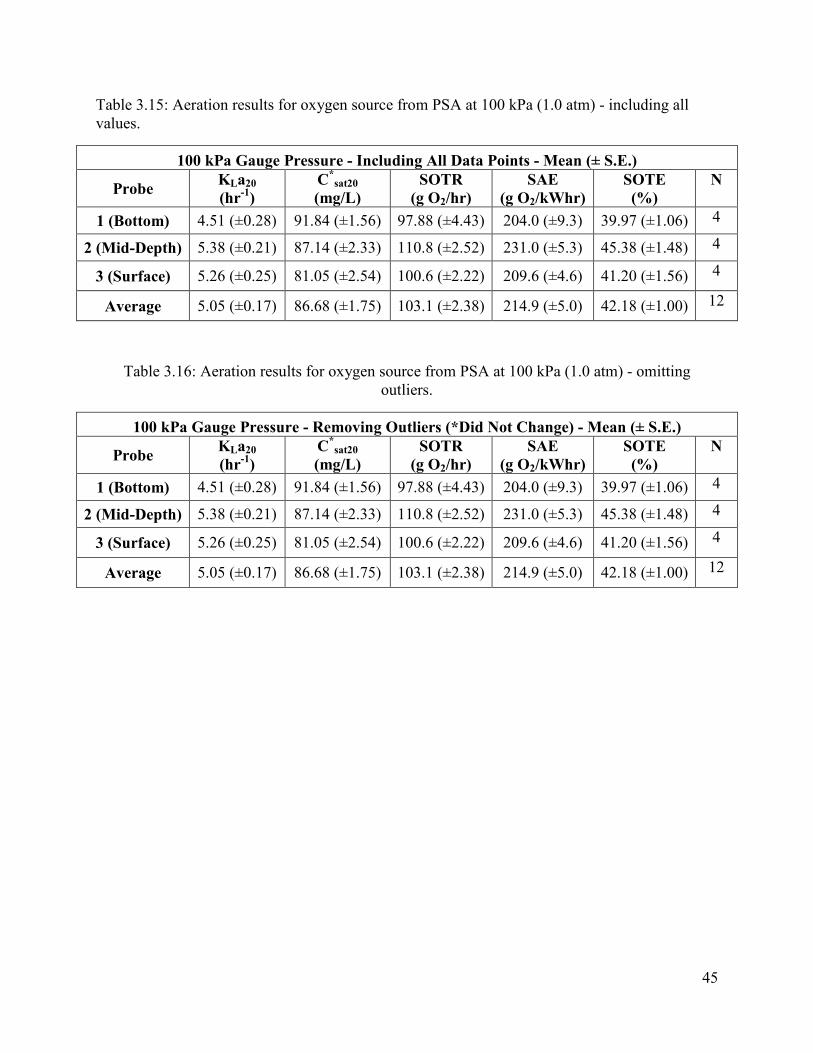
45


values.


Probe KLa20

(hr-1

)

C*

sat20

(mg/L)

SOTR

(g O2/hr)

SAE

(g O2/kWhr)

SOTE

(%)

N

1 (Bottom) 4.51 (±0.28) 91.84 (±1.56) 97.88 (±4.43) 204.0 (±9.3) 39.97 (±1.06) 4

2 (Mid-Depth) 5.38 (±0.21) 87.14 (±2.33) 110.8 (±2.52) 231.0 (±5.3) 45.38 (±1.48) 4

3 (Surface) 5.26 (±0.25) 81.05 (±2.54) 100.6 (±2.22) 209.6 (±4.6) 41.20 (±1.56) 4

Average 5.05 (±0.17) 86.68 (±1.75) 103.1 (±2.38) 214.9 (±5.0) 42.18 (±1.00) 12


outliers.

100 kPa Gauge Pressure - Removing Outliers (*Did Not Change) - Mean (± S.E.)

Probe KLa20

(hr-1

)

C*

sat20

(mg/L)

SOTR

(g O2/hr)

SAE

(g O2/kWhr)

SOTE

(%)

N

1 (Bottom) 4.51 (±0.28) 91.84 (±1.56) 97.88 (±4.43) 204.0 (±9.3) 39.97 (±1.06) 4

2 (Mid-Depth) 5.38 (±0.21) 87.14 (±2.33) 110.8 (±2.52) 231.0 (±5.3) 45.38 (±1.48) 4

3 (Surface) 5.26 (±0.25) 81.05 (±2.54) 100.6 (±2.22) 209.6 (±4.6) 41.20 (±1.56) 4

Average 5.05 (±0.17) 86.68 (±1.75) 103.1 (±2.38) 214.9 (±5.0) 42.18 (±1.00) 12

46


values.


Probe KLa20

(hr-1

)

C*

sat20

(mg/L)

SOTR

(g O2/hr)

SAE

(g O2/kWhr)

SOTE

(%)

N

1 (Bottom) 3.07 (±0.22) 106.0 (±4.73) 77.76 (±2.70) 152.9 (±6.2) 32.68 (±1.56) 4

2 (Mid-Depth) 4.70 (±0.26) 94.70 (±5.71) 106.4 (±4.08) 208.8 (±6.4) 44.57 (±1.12) 4

3 (Surface) 4.53 (±0.69) 91.73 (±1.99) 100.2 (±16.0) 197.7 (±33.6) 42.15 (±7.04) 4

Average 4.10 (±0.26) 97.46 (±2.17) 94.75 (±4.34) 186.5 (±8.5) 39.80 (±1.81) 12


outliers.


Probe KLa20

(hr-1

)

C*

sat20

(mg/L)

SOTR

(g O2/hr)

SAE

(g O2/kWhr)

SOTE

(%)

N

1 (Bottom)* 3.26 (±0.16) 102.9 (±5.16) 80.43 (±0.60) 158.7 (±2.9) 34.03 (±1.10) 3

2 (Mid-Depth) 4.70 (±0.26) 94.70 (±5.71) 106.4 (±4.08) 208.8 (±6.4) 44.57 (±1.12) 4

3 (Surface)* 3.84 (±0.13) 91.29 (±2.74) 84.20 (±0.79) 164.0 (±1.2) 35.13 (±0.77) 3

Average* 4.01 (±0.23) 96.15 (±3.00) 91.93 (±4.23) 180.3 (±8.2) 38.57 (±1.72) 10

47


values.


Probe KLa20

(hr-1

)

C*

sat20

(mg/L)

SOTR

(g O2/hr)

SAE

(g O2/kWhr)

SOTE

(%)

N

1 (Bottom) 4.07 (±0.07) 119.5 (±3.10) 115.1 (±1.76) 217.8 (±2.5) 45.59 (±0.68) 4

2 (Mid-Depth) 3.02 (±0.54) 123.7 (±6.78) 85.22 (±10.5) 161.6 (±21.2) 35.49 (±4.30) 4

3 (Surface) 3.68 (±0.17) 106.3 (±2.15) 92.58 (±4.17) 175.5 (±9.4) 36.72 (±2.05) 4

Average 3.59 (±0.18) 116.5 (±2.90) 97.63 (±4.59) 185.0 (±9.0) 39.27 (±1.88) 12


outliers.


Probe KLa20

(hr-1

)

C*

sat20

(mg/L)

SOTR

(g O2/hr)

SAE

(g O2/kWhr)

SOTE

(%)

N

1 (Bottom) 4.07 (±0.07) 119.5 (±3.10) 115.1 (±1.76) 217.8 (±2.5) 45.59 (±0.68) 4

2 (Mid-

Depth)* 4.06 (±0.22) 110.3 (±2.87) 105.6 (±2.99) 201.7 (±5.9) 41.81 (±2.06)

3

3 (Surface) 3.68 (±0.17) 106.3 (±2.15) 92.58 (±4.17) 175.5 (±9.4) 36.72 (±2.05) 4

Average* 3.92 (±0.10) 112.2 (±2.31) 104.3 (±3.46) 198.0 (±3.5) 41.33 (±1.48) 11

In computing the overall average of the aeration column, there was a possibility of 60 data points

(3 probes x 4 replicates x 5 test pressures). Applying the outlier rule resulted in the removal of 6

outlying data points, or 10% of the overall data collected for PSA oxygen. Two were from probe

1, 2 were from probe 2, and 2 were from probe 3. The minimum number of samples used to

compute the mean at each pressure was at least 10.

The trends depicted by air as the oxygen source were not as apparent when PSA oxygen was

utilized. KLa20 still decreased with increasing pressure and C*sat20 still increased. However, SOTR

shows very little change and remained nearly constant over the range of pressures tested. Since

SOTR is the primary input for the SOTE calculation, SOTE remained relatively constant over

the range of pressures, as well. SAE showed a slight decrease, stemming from the higher power

required to produce PSA oxygen at higher pressures.

48

Figures 3.6 - Figure 3.10 are plots of the means for each parameter along with the error bar and

indicate the trends that occurred. The data plotted in the figures was the data that excluded the

six outlier points.

Figure 3.6: Overall PSA oxygen mass transfer coefficient.

The overall mass transfer coefficient decreased with increasing pressure. Similar to the results

obtained for air, KLa20 decreased approximately 0.5 fold over the pressure range. One possible

cause for the decrease in KLa20 values, similarly to air, is that the increased pressure decreases the

rise velocity of the bubbles and, thus, the turbulence in the water column.

0.00

1.00

2.00

3.00

4.00

5.00

6.00

7.00

8.00

9.00

0 50 100 150 200 250

KLa

20

(hr

-1)

Pressure (kPa)

Average PSA Mass Transfer Coefficient, KLa20

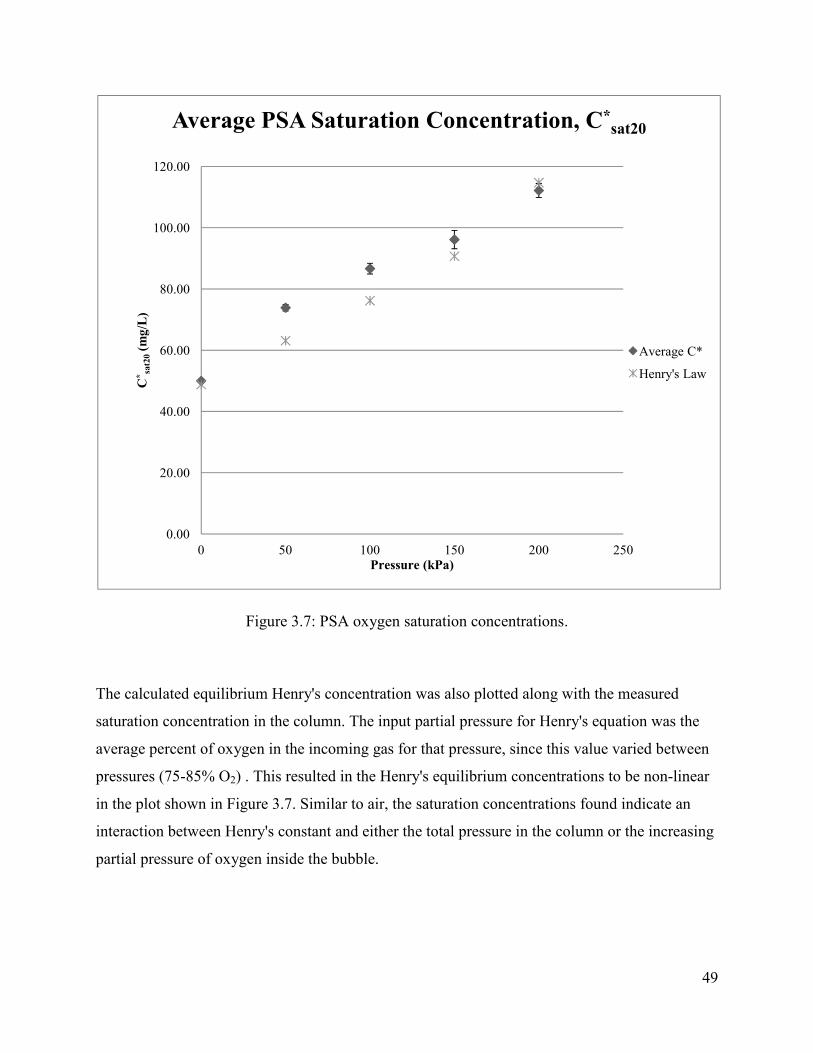
49

Figure 3.7: PSA oxygen saturation concentrations.

The calculated equilibrium Henry's concentration was also plotted along with the measured

saturation concentration in the column. The input partial pressure for Henry's equation was the

average percent of oxygen in the incoming gas for that pressure, since this value varied between

pressures (75-85% O2) . This resulted in the Henry's equilibrium concentrations to be non-linear

in the plot shown in Figure 3.7. Similar to air, the saturation concentrations found indicate an

interaction between Henry's constant and either the total pressure in the column or the increasing

partial pressure of oxygen inside the bubble.

0.00

20.00

40.00

60.00

80.00

100.00

120.00

0 50 100 150 200 250

C*sa

t20

(mg

/L)

Pressure (kPa)

Average PSA Saturation Concentration, C*sat20

Average C*

Henry's Law

50

Figure 3.8: PSA oxygen standard oxygen transfer rate.

Interestingly, Figure 3.8 shows the oxygen transfer rate (SOTR) did not increase nor decrease but

in fact remained relatively constant over the course of the experiments. This would indicate that

the physical transferability of oxygen across a water-bubble interface did not change with respect

to pressure.

0.00

20.00

40.00

60.00

80.00

100.00

120.00

0 50 100 150 200 250

SO

TR

(g

O2/h

r)

Pressure (kPa)

Average PSA SOTR

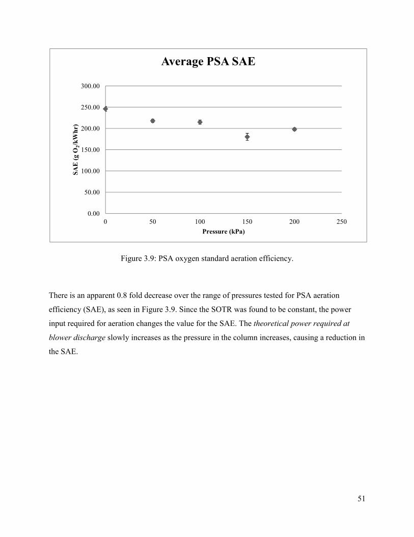
51

Figure 3.9: PSA oxygen standard aeration efficiency.

There is an apparent 0.8 fold decrease over the range of pressures tested for PSA aeration

efficiency (SAE), as seen in Figure 3.9. Since the SOTR was found to be constant, the power

input required for aeration changes the value for the SAE. The theoretical power required at

blower discharge slowly increases as the pressure in the column increases, causing a reduction in

the SAE.

0.00

50.00

100.00

150.00

200.00

250.00

300.00

0 50 100 150 200 250

SA

E (

g O

2/k

Wh

r)

Pressure (kPa)

Average PSA SAE

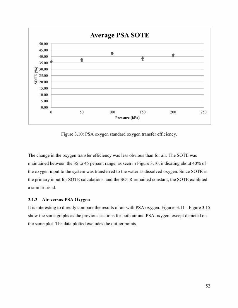
52

Figure 3.10: PSA oxygen standard oxygen transfer efficiency.

The change in the oxygen transfer efficiency was less obvious than for air. The SOTE was

maintained between the 35 to 45 percent range, as seen in Figure 3.10, indicating about 40% of

the oxygen input to the system was transferred to the water as dissolved oxygen. Since SOTR is

the primary input for SOTE calculations, and the SOTR remained constant, the SOTE exhibited

a similar trend.

3.1.3 Air-versus-PSA Oxygen

It is interesting to directly compare the results of air with PSA oxygen. Figures 3.11 - Figure 3.15

show the same graphs as the previous sections for both air and PSA oxygen, except depicted on

the same plot. The data plotted excludes the outlier points.

0.00

5.00

10.00

15.00

20.00

25.00

30.00

35.00

40.00

45.00

50.00

0 50 100 150 200 250

SO

TE

(%

)

Pressure (kPa)

Average PSA SOTE

53

Figure 3.11: Overall mass transfer coefficient for air and PSA oxygen.

The mass transfer coefficient was found to be very similar between air and PSA oxygen, seen in

Figure 3.11. The PSA oxygen only had a slightly higher transfer coefficient, most notably at

atmospheric pressure. Additionally, both gas sources trend in a similar fashion, decreasing with

increasing pressure. The similar transfer coefficients indicate that the amount of oxygen inside

the bubble has very little affect on the ability of the oxygen to transfer across the water-bubble

interface. These results contradict other data published within Civil Engineering, such as Ashley

(2002) and Kowsari (2008). Ashley (2002) and Kowsari (2008) both found the mass transfer

coefficient to be substantially larger for PSA oxygen when compared to the air mass transfer

coefficient. The reason for the discrepancy is primarily based on the method for parameter

estimation, non-linear regression used in this research versus the log-deficit method used by

Ashley (2002) and Kowsari (2008). This will be elaborated on further in the discussion.

0.00

1.00

2.00

3.00

4.00

5.00

6.00

7.00

8.00

9.00

0 50 100 150 200 250

KLa

20

(hr

-1)

Pressure (kPa)

Average Air-PSA KLa20

Air

PSA

54

Figure 3.12: Saturation concentration for air and PSA oxygen.

As was expected, the saturation concentration obtained for PSA oxygen was significantly higher

than what was obtained for air, seen in Figure 3.12. The average difference between PSA oxygen

and air saturation concentrations was 3.9 fold, which correlates to the 80% PSA oxygen versus

21% air (3.8-fold).

0.00

20.00

40.00

60.00

80.00

100.00

120.00

0 50 100 150 200 250

C*sa

t20

(mg

/L)

Pressure (kPa)

Average Air-PSA Saturation Concentration,

C*sat20

Air

PSA

55

Figure 3.13: Standard oxygen transfer rate for air and PSA oxygen.

The oxygen transfer rate (SOTR), seen in Figure 3.13, was found to be near constant for PSA

oxygen, with no apparent trend. The SOTR for air seemed to have a slightly positive linear trend;

however, the error bars that can be seen in Figure 3.3 indicate that the SOTR may also be closer

to a relatively constant value. The SOTR is significantly larger for PSA oxygen than air,

increasing by approximately 5 fold over the range of pressures tested.

0.00

20.00

40.00

60.00

80.00

100.00

120.00

0 50 100 150 200 250

SO

TR

(g

O2/H

r)

Pressure (kPa)

Average Air-PSA SOTR

Air

PSA

56

Figure 3.14: Standard aeration efficiency for air and PSA oxygen.

The standard aeration efficiency (SAE), seen in Figure 3.14, was the only parameter found to be

more advantageous for aeration with air. This is simply due to the higher amount of energy

required for PSA oxygen production. In both instances, the SAE did not indicate significant

change over the pressure ranges tested. The maximum difference between air and PSA oxygen

was found to be a 5.8 fold increase for air, at 150 kPa.

0.00

200.00

400.00

600.00

800.00

1000.00

1200.00

0 50 100 150 200 250

SA

E (

g O

2/k

Wh

)

Pressure (kPa)

Average Air-PSA SAE

Air

PSA

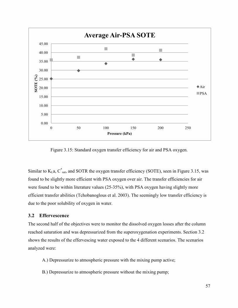
57

Figure 3.15: Standard oxygen transfer efficiency for air and PSA oxygen.

Similar to KLa, C*sat, and SOTR the oxygen transfer efficiency (SOTE), seen in Figure 3.15, was

found to be slightly more efficient with PSA oxygen over air. The transfer efficiencies for air

were found to be within literature values (25-35%), with PSA oxygen having slightly more

efficient transfer abilities (Tchobanoglous et al. 2003). The seemingly low transfer efficiency is

due to the poor solubility of oxygen in water.

3.2 Effervescence

The second half of the objectives were to monitor the dissolved oxygen losses after the column

reached saturation and was depressurized from the superoxygenation experiments. Section 3.2

shows the results of the effervescing water exposed to the 4 different scenarios. The scenarios

analyzed were:

A.) Depressurize to atmospheric pressure with the mixing pump active;

B.) Depressurize to atmospheric pressure without the mixing pump;

0.00

5.00

10.00

15.00

20.00

25.00

30.00

35.00

40.00

45.00

0 50 100 150 200 250

SO

TE

(%

)

Pressure (kPa)

Average Air-PSA SOTE

Air

PSA

58

C.) Depressurize to 50 kPa (0.5 atmospheres) with the mixing pump active;

D.) Depressurize to 50 kPa (0.5 atmospheres) without the mixing pump active.

The purpose of monitoring these four differing environments was to determine whether or not

certain environmental factors play a role in releasing oxygen from supersaturated water or if the

water effervesces spontaneously and returns to saturation at normal temperature and pressure.

Additionally, since there is no data currently available on the effervescence of oxygen in water

and how this phenomena interacts with other factors, this data would provide the first such

database.

Tables 3.21 - Table 3.24 depict the percent loss of dissolved oxygen after 20 minutes of

effervescence from the air superoxygenation experiments. Figure 3.16 shows the percent loss of

D.O. on a bar chart. The percent loss was determined from the percent difference in the

concentration measured by the probes while the column was still pressurized and the

concentration measured 20 minutes after depressurizing. The average for the three probes was

then found to determine the mean dissolved oxygen lost within the column. Since the tests

conducted at 50 kPa could not be depressurized to 50 kPa, scenarios A and B were repeated.

Effervescence was not tested at atmospheric conditions (0 kPa) because initial tests found that

the column did not effervesce at atmospheric conditions. Since the pressure and temperature

remained the same in the column, the saturation concentration did not change.

Table 3.21: Air effervescence at 50 kPa (0 atm).

50 kPa - Air

Scenario Average % Effervescent

Loss (± S.E.) N

A 19.6 (± 1.3) 6

B 7.3 (± 3.1) 6

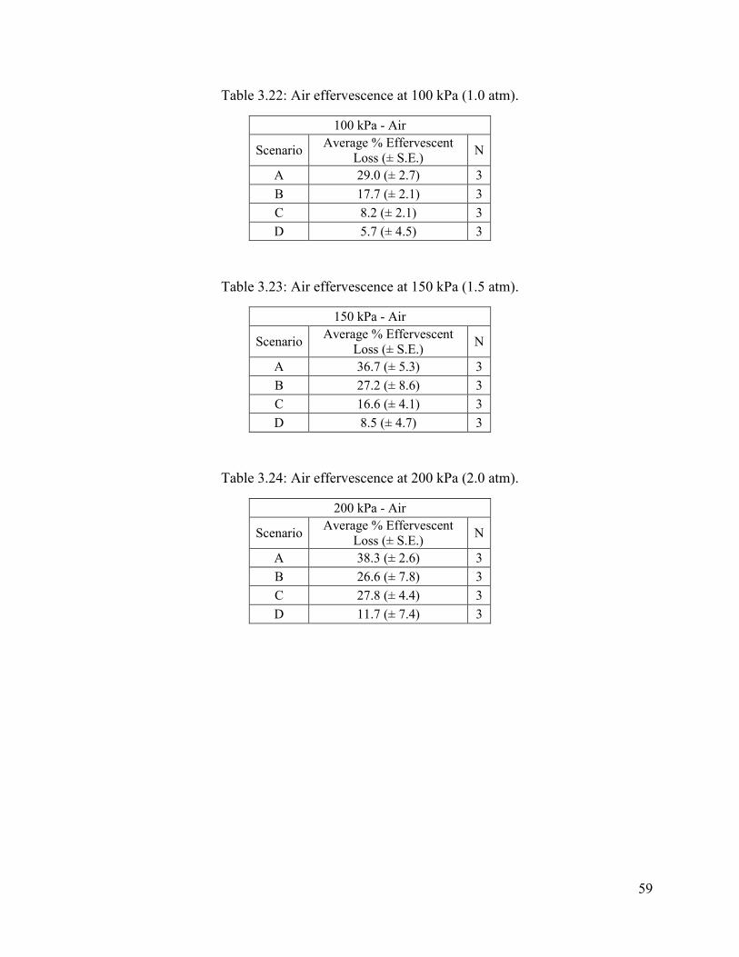
59

Table 3.22: Air effervescence at 100 kPa (1.0 atm).

100 kPa - Air


Loss (± S.E.) N

A 29.0 (± 2.7) 3

B 17.7 (± 2.1) 3

C 8.2 (± 2.1) 3

D 5.7 (± 4.5) 3


150 kPa - Air


Loss (± S.E.) N

A 36.7 (± 5.3) 3

B 27.2 (± 8.6) 3

C 16.6 (± 4.1) 3

D 8.5 (± 4.7) 3


200 kPa - Air


Loss (± S.E.) N

A 38.3 (± 2.6) 3

B 26.6 (± 7.8) 3

C 27.8 (± 4.4) 3

D 11.7 (± 7.4) 3

60

Figure 3.16: Air effervescent loss for scenarios A-D.

Tables 3.25 - Table 3.28 show the effervescent loss for PSA oxygen and Figure 3.17 depicts the

data on a bar chart.

Table 3.25: PSA oxygen effervescence at 50 kPa (0.5 atm).

50 kPa - PSA


Loss (± S.E.) N

A 26.1 (± 2.0) 6

B 23.1 (± 1.3) 6

0

5

10

15

20

25

30

35

40

45

50 100 150 200

Per

cen

t L

oss

(%

)

Starting Pressure (kPa)

Air - Effervescent Loss (20 minutes)

Pump On - 0 kpa Release

Pump Off - 0 kpa Release


Pump Off - 50 kPa Release

61


100 kPa - PSA


Loss (± S.E.) N

A 40.1 (± 2.4) 3

B 27.6 (± 0.6) 3

C 14.1 (± 0.5) 3

D 14.2 (± 4.3) 3


150 kPa - PSA


Loss (± S.E.) N

A 47.3 (± 2.2) 3

B 34.3 (± 3.6) 3

C 28.2 (± 2.8) 3

D 21.9 (± 1.4) 3


200 kPa - PSA


Loss (± S.E.) N

A 46.7 (± 1.9) 3

B 25.6 (± 3.0) 2

C 42.4 (± 1.7) 2

D 20.9 (± 1.6) 3

62

Figure 3.17: PSA effervescent loss for scenarios A-D.

Figures 3.16 and Figure 3.17 both show that for both increasing pressure differential (i.e. the

difference between column pressure and column release pressure), the amount of oxygen that

effervesces from the water increases. This was due to the saturation concentration within the

column changing more dramatically. For example, at 150 kPa, the saturation concentration was

found to be 96 mg/L, while at 200 kPa, the saturation concentration was found to be 112 mg/L.

Hence, more oxygen tries to escape the dissolved phase when going from 200 kPa to

atmospheric than going from 150 kPa to atmospheric. This can also be seen at each pressure

individually, where more D.O. is lost when the column is released to atmospheric pressure, than

when released to 50 kPa. The mixing pump was found to have an effect, as a more turbulent

regime in the water caused more oxygen to effervesce from the system.

0

5

10

15

20

25

30

35

40

45

50

50 100 150 200

Per

cen

t L

oss

(%

)

Starting Pressure (kPa)

PSA - Effervescent Loss (20 minutes)





63

3.3 Quality Control

Since the database primarily relies on the dependability of the OxyGuard probes, additional

techniques were desired for oxygen measurement. Unfortunately, there is no robust method for

determining the amount of oxygen in the water at the high pressures on a molecular level. That is

what certain methods, such as the Winkler titration, provide. These methods quantify the exact

number of moles of oxygen dissolved in the water. However, it was not feasible to titrate the

water under pressure in the test column. Therefore, utilizing this method at atmospheric pressure,

with some gross assumptions, was used to estimate the amount of dissolved oxygen in the

column.

A tap was placed at about the 5-foot (1.5 m) depth mark of the column with a 1/8-inch (3.2 mm)

ball valve connected to one foot (0.3 m) of 1/8-inch (3.2 mm) tubing. The column underwent

normal deoxygenation procedures to remove the initial dissolved oxygen from the water. This

water was used as dilution water and 225 mL were measured into a 300 mL BOD bottle from the

tap. Then an experiment was conducted as a "blank" using nitrogen as the aeration gas. The

column was pressurized to 50 kPa and allowed to reach saturation and then the remaining 75 mL

in the BOD bottle was filled from the tap in the column. This was repeated for the 5 test

pressures providing "blanks" at each pressure. Then typical experiments using PSA oxygen were

conducted, similar to the nitrogen, where 75 mL of the superoxygenated water was added to a

BOD bottle containing 225 mL of deoxygenated water. Two duplicates were collected at each

test pressure. Even though the sample in the BOD bottle did not contain the same amount of

D.O. as what was in the column, the D.O. in the BOD bottle and a dilution factor were used to

estimate the D.O. in the superoxygenated stream. Additionally, the diluted D.O. concentration

provided values for the working range of the Winkler titration (0-20 mg/L).

3.3.1 Winkler Titration

The Winkler titration provides a precise measurement of the amount of oxygen molecules in the

water sample. The titration procedure is based on the oxidizing property of D.O. The titration

used was the azide modification, as it was found most applicable to the source water in this

research.

During the azide modification, according to Standard Methods, 1 mL of manganous sulfate

solution (MnSO4) was added to the 300 mL of sample in the BOD bottle, followed by 1 mL of

64

alkali-iodide-azide reagent (American Water Works Association et al. 1992). This created a

precipitate in the BOD bottle, and once the precipitate settled in the sample, 1 mL of

concentrated sulfuric acid (H2SO4) was added. The solution was then mixed until the precipitate

was dissolved by the sulfuric acid. A volume of 200 mL of the mixture was then titrated with

0.025 Molar sodium thiosulfate (Na2S2O3) to a pale yellow color. A few drops of starch solution

was then added to turn the solution to a blue color and titration continued until the blue color

disappeared. Each 1 mL of sodium thiosulfate added to the solution corresponds to 1 mg/L D.O.

in the sample.

3.3.2 Results

The dissolved oxygen found in the samples by way of a Winkler titration is shown in Table 3.29:

Table 3.29: Winkler titration D.O. values.

Sample Pressure

(kPa) A

(mg/L) B

(mg/L) Blank

(mg/L) Temp °C

50 7.9 9.35 0 21.1

100 12.8 13.55 0 21.1

150 13.7 15 0 21.1

200 16.6 17 0 21.1

Sample B was taken a minimum of 5 minutes after Sample A was taken, resulting in the higher

D.O. concentration. The column was allowed to saturate for 15 minutes, once the pressure step

was increased 50 kPa. Since the time of aeration at the 50 kPa pressure was 40 minutes, and

using the experimental KLa values obtained, it is assumed that the column was at least at 95%

saturation by the time sample B was collected. Using a dilution factor of 4 (i.e., 300 mL Total/75

mL Sample) the D.O. in the reactor at each pressure can be calculated and is shown in Table

3.30.

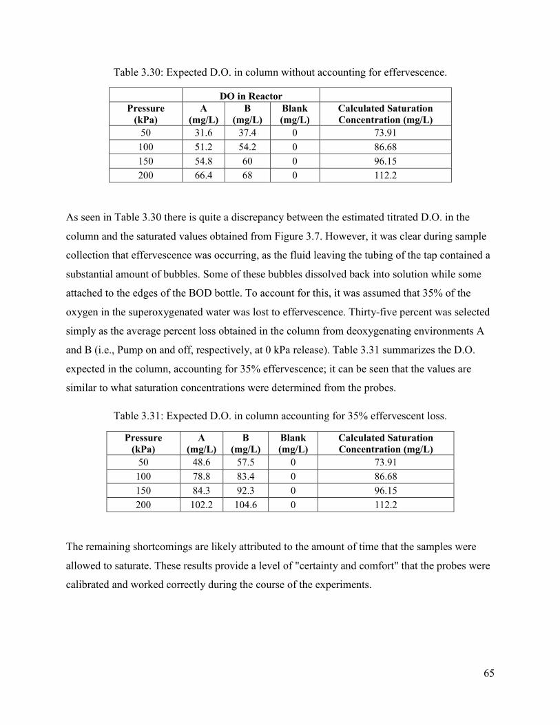
65

Table 3.30: Expected D.O. in column without accounting for effervescence.

DO in Reactor

Pressure

(kPa) A

(mg/L) B

(mg/L) Blank

(mg/L) Calculated Saturation

Concentration (mg/L)

50 31.6 37.4 0 73.91

100 51.2 54.2 0 86.68

150 54.8 60 0 96.15

200 66.4 68 0 112.2

As seen in Table 3.30 there is quite a discrepancy between the estimated titrated D.O. in the

column and the saturated values obtained from Figure 3.7. However, it was clear during sample

collection that effervescence was occurring, as the fluid leaving the tubing of the tap contained a

substantial amount of bubbles. Some of these bubbles dissolved back into solution while some

attached to the edges of the BOD bottle. To account for this, it was assumed that 35% of the

oxygen in the superoxygenated water was lost to effervescence. Thirty-five percent was selected

simply as the average percent loss obtained in the column from deoxygenating environments A

and B (i.e., Pump on and off, respectively, at 0 kPa release). Table 3.31 summarizes the D.O.

expected in the column, accounting for 35% effervescence; it can be seen that the values are

similar to what saturation concentrations were determined from the probes.

Table 3.31: Expected D.O. in column accounting for 35% effervescent loss.

Pressure

(kPa) A

(mg/L) B

(mg/L) Blank

(mg/L) Calculated Saturation

Concentration (mg/L)

50 48.6 57.5 0 73.91

100 78.8 83.4 0 86.68

150 84.3 92.3 0 96.15

200 102.2 104.6 0 112.2

The remaining shortcomings are likely attributed to the amount of time that the samples were

allowed to saturate. These results provide a level of "certainty and comfort" that the probes were

calibrated and worked correctly during the course of the experiments.

66

4 Discussion

4.1 Gas Transfer Theory

First, it is useful to briefly review the gas transfer theory and elaborate further from what was

described in the literature review. As discussed earlier, several theories describe the mass

transfer of gas into liquid, stemming from the research by Lewis and Whitman (1924) into the

Two-Film theory and the Film Penetration theory by Higbie (1935), who theorized mixing of the

water caused some gas transfer. Danckwertz (1951) carried the Film Penetration theory further,

indicating the importance of surface renewal at the bubble-liquid interface. Many of the theories

are approximations and Dobbins (1964) has proposed the theory that appears to best describe the

gas transfer process (Ashley 2002). Dobbins' (1964) theory is a combination of the Two-Film

theory (Lewis and Whitman 1924) and the Surface Renewal theory (Danckwertz 1951).

Dobbins (1964) suggested that oxygen molecules are transported to the liquid film at the bubble

surface by a partial pressure gradient in the bubble and a concentration gradient in the liquid

phase. The oxygen molecules that are transported to the liquid film cause saturation conditions at

the bubble-water interface (Ashley 2002). Due to the poor solubility of oxygen in water, the

transport of gaseous oxygen through the bubble proceeds much more rapidly than through the

liquid film (Eckenfelder 1959).

The transport of oxygen molecules through the liquid film occurs from molecular diffusion and

it is presumed that the interface is at saturation; therefore, all of the resistance to oxygen passing

the interface into the water is from the molecular diffusion across the liquid film (Eckenfelder

1959). The oxygen that passes through this thin liquid film is then mixed into the bulk water by

diffusion and convection currents (Ashley 2002). Convective mass transfer is described by the

flux of a molecule (Fick's law) from a surface to the bulk phase, and a convective mass transfer

coefficient is used to represent the molecular and eddy diffusivities of the molecule (Geankoplis

2009). The mass transfer occurs from a driving force, or concentration gradient, existing between

the interface and bulk liquid (Geankoplis 2009). This can be seen visually in Figure 4.1 (from

Ashley 2002).

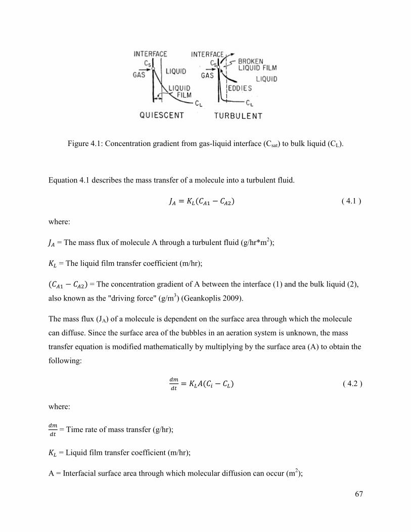
67

Figure 4.1: Concentration gradient from gas-liquid interface (Csat) to bulk liquid (CL).

Equation 4.1 describes the mass transfer of a molecule into a turbulent fluid.

f = " − ( 4.1 )

where:

f = The mass flux of molecule A through a turbulent fluid (g/hr*m2);

= The liquid film transfer coefficient (m/hr);

" − = The concentration gradient of A between the interface (1) and the bulk liquid (2),

also known as the "driving force" (g/m3) (Geankoplis 2009).

The mass flux (JA) of a molecule is dependent on the surface area through which the molecule

can diffuse. Since the surface area of the bubbles in an aeration system is unknown, the mass

transfer equation is modified mathematically by multiplying by the surface area (A) to obtain the

following:

*2* = ^- − ( 4.2 )

where:

*2* = Time rate of mass transfer (g/hr);

= Liquid film transfer coefficient (m/hr);

A = Interfacial surface area through which molecular diffusion can occur (m2);

68

- = Interface concentration, i.e. saturation concentration (C*sat) of dissolved oxygen between

liquid and gas bubble (mg/L);

= Average concentration of dissolved oxygen in the bulk liquid (mg/L) (Mavinic and Bewtra

1974).

The mass transfer equation can be changed to concentration units by dividing through by the

volume (V) of the liquid:

*1* =

"g*2* =

g - − = - − ( 4.3 )

where:

*1* = Time rate of oxygen concentration transfer, i.e. SOTR (mg/L*hr);

V = Volume of the liquid (m3);

A/V = a = Interfacial surface area of the bubble through which oxygen can diffuse in a particular

aeration system per unit volume of water (m2/m

3) (Ashley 2002);

KLa = Overall oxygen transfer coefficient (hr -1

).

Due to the impracticality of measuring the liquid film transfer coefficient (KL) and "a" directly, it

has become standard practice to consider the aeration process in terms of the overall oxygen

transfer coefficient (KLa) (Ashley 2002). Equation 4.3 is modified mathematically through

integration to result in Equation 2.1 found in Section 2.4, as is the equation reported in the ASCE

standard.

4.1.1 Applications of Gas Transfer Theory

From Equation 4.3 the primary parameters affecting gas transfer are the oxygen saturation

concentration (Csat or Ci), overall oxygen transfer coefficient (KLa), and the dissolved oxygen

concentration in the bulk liquid (CL).

4.1.1.1 Oxygen Saturation Concentration

The saturation concentration was the primary focus of this research. Increasing the saturation

concentration directly results in increasing the "driving force" for aeration. Increasing the

69

pressure in the column would increase the oxygen saturation concentration and indicate the

effects of increasing C*sat on the driving force for mass transfer. Henry's law correlates the

equilibrium between partial pressure of oxygen in the gas phase and the dissolved oxygen

concentration in the liquid. Henry's constant, and thus the saturation concentration, is controlled

by temperature, pressure, and dissolved solids concentrations. The partial pressure of oxygen in

the gas bubble is affected by the oxygen purity within the bubble and the total pressure at which

the bubble is exposed.

4.1.1.2 Oxygen Transfer Coefficient

Many factors influence the oxygen transfer coefficient, KLa, because several different factors

change both KL and "a" independently as well as synergistically. Several factors affecting the

mass transfer coefficient are:

1.) Water temperature;

2.) Depth of gas release;

3.) Bubble contact time;

4.) Gas bubble size;

5.) Gas flow rate;

6.) Diffuser type and orifice size;

7.) Turbulence in the liquid;

8.) Position of the diffuser;

9.) Aeration tank dimensions;

10.) Presence of dissolved solids and organics (i.e. surfactants) (Mavinic and Bewtra 1974).

Since so many factors influence the mass transfer coefficient, it was necessary to run each

experiment similarly, such that the only factors affecting KLa were related to the pressure in the

column. The same diffusers, gas flow rate, and diffuser positioning were used in these

experiments. Maintaining the same gas flow rate throughout kept the turbulence within the

70

column theoretically similar throughout the experiments. Additionally, tank volume was kept

constant throughout the experiments, along with limiting the amount of dissolved solids present

in the liquid.

4.1.1.3 Dissolved Oxygen Concentration in Bulk Liquid

The oxygen concentration already in the liquid, CL, affects gas transfer by either increasing or

decreasing the driving force for transfer to occur. Hence, as oxygen transfer takes place

throughout an aeration experiment, CL increases, thus decreasing oxygen transfer rate. This

explains why the water needs to be deoxygenated, as per the ASCE standard, prior to each

experiment; starting the driving force at a maximum with CL equal to zero. The total driving

force will be a key factor when analyzing the benefits of using high purity oxygen for aeration

later in the chapter.

4.1.1.4 Factors Affecting Effervescence

On the reverse side of gas transfer, is the loss of dissolved oxygenation due to effervescence, as

the phase equilibrium shifts towards the gaseous phase. When the water is under a certain set of

conditions, i.e. temperature and pressure, the saturation concentration is a certain value for that

temperature and pressure. As soon as the pressure exerted on the water is reduced, the

equilibrium saturation value is reduced as well. Reducing the saturation concentration will cause

some effervescence. However, several other factors affect the effervescence of oxygen from

water. These, among other things, include: the pressure the water is released to, nucleation sites

in the water, and turbulence of the water (Speece 2007).

4.2 Effect of Pressure on Mass Transfer Coefficient

It is clear that, for both air and PSA oxygen, increasing pressure caused the mass transfer

coefficient to decrease. There are mixed results in the literature regarding the effects of pressure

on the overall mass transfer coefficient. Yoshida and Arakawa (1968), Letzel et al. (1999), and

Jin et al. (2004) show that the mass transfer coefficient and/or the liquid film coefficient (KL)

actually increase with increasing pressure. Letzel et al. (1999) showed that, with increasing

system pressure, the gas holdup of the bubble increases as well. This is due to the increase in

system pressure shrinking the bubble size and, thus, decreasing the rise velocity of the bubble in

the water column (Letzel et al. 1999). Yoshida and Arakawa (1968) included a mixer in their

system design and found KL to increase with increasing pressure. However, they found the

71

pressure dependence to be less obvious when the agitator was operated at a higher mixing speed

(Yoshida and Arakawa 1968). Jin et al. (2004) found the mass transfer coefficient to increase

with increasing pressure as well, in an unmixed bubble column. Teramoto et al. (1974) found

that the liquid mass transfer coefficient was independent of increasing system pressure, and

actually remained constant over the course of the experiments.

The discrepancies in the literature can be explained. The primary difference between the results

of Teramoto et al. (1974) and Letzel et al. (1999), Yoshida and Arakawa (1968), and Jin et al.

(2004) is secondary mixing of the column. As Dobbins (1964) stressed, mass transfer is highly

dependent on the surface renewal rate of the bubble-water interface. In the experiments

conducted without a secondary mixing device, the transfer coefficient consistently increased.

This is likely due to the gas holdup from the increased system pressure and the decrease in

bubble size and rise velocity, as found by Letzel et al. (1999). Smaller bubbles increase the

surface area that the oxygen can transfer through, increasing KLa. A lower rise velocity will

increase the contact time between the bubble and water, consequently increasing KLa. However,

a lower rise velocity also induces a less turbulent hydrodynamic regime in the water column; a

lesser hydrodynamic regime would decrease the surface renewal rate and thus KLa. As explained

in Section 4.1.1.2, there are many factors affecting KLa, making KLa unique to each system to

which it is employed. As shown by Teramoto et al. (1974), when an agitator was introduced into

the system, the mass transfer coefficient stayed constant over the range of pressures tested. With

the agitator, the surface renewal rate was increased and could have eliminated any effects of gas

hold up from increased pressure. This was also shown by Yoshida and Arakawa (1968) when, at

the higher mixing speeds, the dependence of KLa on pressure was less apparent.

All of the columns used in the previous examples were not as large as the column used for this

research; the largest was by Jin et al. (2004) at 1.25 m, only one-fifth the column size used for

these experiments. Due to the further distance the bubble must rise in this research, the contact

time and decreased bubble size may not have had as great of an influence on the mass transfer

coefficient as the decreased turbulence over the span of the column height. This could explain

the decrease in the mass transfer coefficient over the increased operating pressures. Additionally,

the mass transfer may not be entirely liquid film controlled.

72

As suggested by Eckenfelder (1959), it is thought that the primary resistance of poorly soluble

gases is due to the liquid film. However, Versteeg et al. (1987) found the gas phase mass transfer

coefficient (Kg) of nitrogen gas to decrease with increasing pressure. This could be another factor

influencing the overall mass transfer coefficient (KLa); if the gas diffusivity in the bubble is

decreasing with increasing pressure, then the renewal rate of oxygen at the interface would

decrease. Since there is such a high "driving force", with superoxygenation, on molecules

leaving the liquid film to the bulk liquid, the gas would be unable to maintain the liquid film at

saturated conditions.

4.2.1 Effect of Differing Gas Purities on Mass Transfer Coefficient

The mass transfer coefficient did not vary greatly between the different purity of gases used.

Figure 3.11 shows that the PSA oxygen only had a slightly larger mass transfer coefficient. This

largely contradicts the work done by Ashley (2002) and Kowsari (2008). Ashley (2002) found

KLa for PSA oxygen to be about 4-6 fold greater than the KLa found for air in a full lift

hypolimnetic aerator. Additionally, in a Speece cone, Ashley (2002) and Kowsari (2008) found

the PSA oxygen KLa to be about 6-8 fold greater than the air KLa value. The difference can be

primarily attributed to the different methods used in parameter estimation.

This research utilized the non-linear regression method for parameter estimation (Section 2.4).

While, Ashley (2002) and Kowsari (2008) each used the log-deficit method for parameter

estimation. The log-deficit method is based on a one parameter linear regression of the log form

of Equation 2.1. Since Equation 2.1 has two unknown parameters, the log-deficit method

requires estimation of the saturation concentration (C*sat) to determine KLa. Ashley (2002) and

Kowsari (2008) conducted experiments until the water reached about 70% saturation, in which

the saturation was determined from air-water D.O. equilibrium tables. However, the issue with

the log-deficit method is that estimating the saturation concentration for PSA oxygen with air-

water saturation tables underestimates the true saturation concentration. As discussed in Section

1.1.3, the higher purity the oxygen gas, the larger the saturation concentration will be, shown by

Henry's law. The current method for determining mass transfer coefficients using the log-deficit

method, requires that the saturation concentration be estimated by averaging three D.O.

measurements, 5 minutes apart, at a starting time of no shorter than 6/ KLa20 (ASCE 2007). The

ASCE standard suggests that KLa will increase 3% for every 1% decrease in estimation of C*sat

73

and, thus, does not recommend using this a priori method of estimating C*sat from D.O.

saturation tables (ASCE 2007). This revised version of the ASCE standard was published after

the research by Ashley (2002) and Kowsari (2008).

Since the non-linear regression method was employed for this research, there was no estimation

of C*sat, and the saturation concentration was, in fact, determined from the Excel model. This

model, discussed in Section 2.4, was coded by Michael Stenstrom (author of the ASCE standard)

and calculated the saturation concentration from a D.O. versus time data input, based on non-

linear regression. The log-deficit method was performed on one randomly selected data set (50

kPa pressure, replicate 'A') for PSA oxygen and air to compare the differences between the log-

deficit and non-linear regression methods. This can be found in Table 4.1 and Table 4.2. Note:

The saturation concentration for the log-deficit method was found from an air-water D.O.

saturation table accounting for pressure by including 50 kPa headspace pressure with the mid-

depth pressure of the water column. The saturation concentration for the non-linear regression

method was determined from the Excel model.

Table 4.1: Log-Deficit versus Non-Linear Regression method for PSA at 50 kPa.

Mass Transfer Coefficient-PSA 50 kPa (Rep 'A')

Bottom

(hr-1

) Mid-Depth

(hr-1

) Surface

(hr-1

)

Saturation

Concentration

(mg/L)

Log-Deficit 32 30 15 18.1

Non-Linear Regression 5.0 4.3 4.5 73

Table 4.2: Log-Deficit versus Non-Linear Regression method for air at 50 kPa.

Mass Transfer Coefficient-Air 50 kPa (Rep 'A')

Bottom

(hr-1

) Mid-Depth

(hr-1

) Surface

(hr-1

)

Saturation

Concentration

(mg/L)

Log-Deficit 5.8 5.9 6.2 18.1

Non-Linear Regression 5.19 5.36 5.67 17.4

As can be seen in Table 4.1 and Table 4.2, the log-deficit method largely overestimates the mass

transfer coefficient when using a tabulated D.O. saturation concentration value. Even though the

difference between PSA and air mass transfer coefficients in this research are significantly

74

different than those found in the literature, the oxygen transfer rates (SOTR) are similar, which

will be discussed in Section 4.4.

Therefore, the similarity between the mass transfer coefficients of air and PSA oxygen in this

research, found using the robust non-linear regression method, indicates that the mass transfer

coefficient is independent of the gas composition in the bubble. Since the gas flow rates, column

volume, and bubble diffusers were the same in both experiments, the A/V ratio in Equation 4.3

should be similar, thus, not affecting KLa. The different densities between high purity oxygen

(1.4277 g/L) and air (1.2927 g/L) at standard conditions could slightly change the bubble rise

velocity and, thus, the hydrodynamic conditions and surface renewal rate within the column

(Versteeg et al. 1987). This could explain the slightly higher KLa for PSA oxygen over the

pressures tested.

4.3 Effect of Pressure on Saturation Concentration

As was expected, the saturation concentration (C*

sat) increased with increasing pressure. This is

due to the equilibrium between the partial pressure of oxygen and the dissolved oxygen in water,

as described by Henry's law. However, it can be seen that Henry's constant itself may not be

entirely independent of the pressure in the system. This can be explained by gas-liquid

equilibrium thermodynamics.

4.3.1 Effect of Henry's Constant

It is well established that, for sparingly soluble gases, the solubility is proportional to the

gaseous-phase fugacity, or partial pressure. This is denoted by Equation 4.4:

M = ( 4.4 )

where:

M= Gas fugacity, partial pressure (atm);

K = Proportionality constant (atm);

X2 = Mol fraction of solute in water (mole fraction) (Wilhelm et al. 1977).

The proportionality constant, K, is directly related to Henry's constant by the activity coefficient

of dissolved oxygen in water. The activity coefficient is defined as a factor used in

75

thermodynamics to account for deviations from ideal behavior in a mixture (Kyle 1999). In an

ideal mixture, the interactions between the same chemical species are the same and the volume

variation in mixing is zero (Kyle 1999). This is denoted by Equation 4.5:

= h ( 4.5 )

where:

K = Proportionality constant (atm);

h = Activity coefficient of dissolved oxygen (unitless);

H = Henry's constant (atm) (Wilhelm et al. 1977).

For dilute solutions, it is commonly assumed that the activity coefficient approaches unity and

can be disregarded from equilibrium equations. Additionally, on the vapor side of the equation

there exists a fugacity coefficient. The fugacity coefficient relates the behavior of the gas in

reality versus if the gas were ideal (Kyle 1999). According to the Lewis fugacity rule, at

temperatures below the boiling point of water and within a few atmospheres of pressure, the

fugacity coefficient is independent of the gas composition (Wilhelm et al. 1977). Therefore,

fugacity of the gas can just be assumed as the partial pressure of that gas, i.e. the fugacity

coefficient approaches unity.

The deviations of the experimental saturation concentrations obtained can be attenuated to these

assumptions that form the basis of Henry's law. While subtle, the saturation concentrations seem

to deviate from Henry's equilibrium line with increasing pressure and increasing gas purity. This

indicates non-unity values for the activity coefficient and fugacity coefficient, affecting the

equilibrium that exists between gaseous and aqueous oxygen.

The saturation concentration, in addition to increasing over the pressure ranges, increased when

using PSA oxygen as opposed to air. The difference between the saturation concentrations was

found, on average, to be 3.71 fold greater for PSA oxygen, consistent with the average percent

oxygen in PSA when compared to air (80%/21% = 3.81). This is expected as the partial pressure

within the gas bubble is increasing, thus the D.O. equilibrium concentration must increase by

way of gas-liquid equilibrium.

76

4.4 Effect of Pressure on SOTR

The effect of pressure on the oxygen transfer rate is seemingly negligible, for both PSA and air.

The results indicated that, as pressure increased, the rate at which oxygen transfered into the

water was the same. Eckenfelder (1952) suggested that the effect of temperature on SOTR is also

constant. As temperature increases, so does KLa. Conversely, as the temperature increases the

saturation concentration decreases. Reviewing Equation 2.4, the SOTR is the product of the

volume, mass transfer coefficient, and the saturation concentration of the water. With increasing

(or decreasing) temperature, the opposite trends of KLa and C*sat tend to cancel each other out,

resulting in a constant value over different temperature ranges (Eckenfelder 1952).

This research suggests similar effects over changing pressure conditions. With increasing

pressure, the saturation concentration will increase; therefore, KLa must decrease to maintain the

oxygen transfer rate at a constant value. This suggests that for a given system, the ability to

transfer oxygen into the water will be the same no matter what the conditions give. The

exception would be increasing the purity of the oxygen in the feed gas.

This research shows a 5 fold increase in the SOTR from air to PSA oxygen. Interestingly, this

increase is greater than the increase of saturation concentrations between air and PSA oxygen

(~3.7 fold). This would indicate that the ability of oxygen to transfer to the aqueous phase

increases slightly with increasing purity of oxygen in the bubble. Since oxygen transfer rates are

dependent on each aeration system specifically, it is difficult to directly compare SOTR with

literature values. However, Colt et al. (1993) found values ranging from 50-800 g O2/hr; Ashley

(2002) found values easily surpassing 100 g O2/hr in a full lift hypolimnetic aerator; and Ashley

et al. (2014) found SOTR values up to 100 g O2/hr when using a Speece cone. The data in this

research was found to be well within those ranges.

4.5 Effect of Pressure on SAE

The aeration efficiency remained close to a constant value as the pressure in the system increased

for air, while a slight decrease for PSA oxygen was observed. Recalling Equation 2.8, the SAE is

simply the SOTR divided by the power input of the system. As discussed in Section 4.4, the

SOTR remained constant throughout the experiments and the change in power requirements at

each pressure is not significant. For example, the power required for air production at 200 kPa

was 0.026 kW versus 0.017 kW at 0 kPa, 0.7 fold decrease. The power required for PSA

77

production at 200 kPa was 0.54 kW, as opposed to 0.41 kW at 0 kPa, a 0.8 fold decrease. The

decrease in power requirement for PSA oxygen (0.8 fold) is the same as the decrease in SAE

over the range of pressures tested. The change is more apparent in PSA oxygen than in air,

simply because of A.) the higher pressure required for the PSA unit (105 psia vs. 60 psia) and B.)

the higher mass flow rate of air required to the PSA unit (15.9:1). Aeration becomes more power

intensive at the higher pressures, due to pressurizing the headspace, increasing the value of p2 in

Equation 2.9 and, thus, increasing the total power requirement.

The aeration efficiency is considerably greater for air, compared to PSA oxygen. This is the only

parameter in which air improved over PSA oxygen. This is expected since the power required to

produce high purity oxygen can be substantially greater than the power required to compress air.

This was represented in Equation 2.9 by including the published ratio for air input to oxygen

output of the AirSep unit (i.e., 15.9:1) (AirSep Corporation 2002). The expansion ratio indicates

that it requires 15.9 times as much power to produce oxygen as opposed to air. The SAE for air

was found to be approximately 5 fold greater than for PSA oxygen (at 150 kPa). Similar results

were obtained by Ashley (2002), where, in a full lift hypolimnetic aerator, it was found that air

had a better SAE by approximately 3-5 fold. However, these results can be misleading as air is

limited by the maximum amount of oxygen it can deliver to the water, affecting the driving

force, and the rate at which it can deliver the oxygen. Additionally, new aeration technologies

may improve the SAE for high purity oxygen over the use of typical diffused aeration.

For example, research by Ashley (2002) and Kowsari (2008) showed that, with using a Speece

cone, the SAE was substantially higher for PSA oxygen as opposed to air. Results obtained show

a 5-8 fold increase in SAE for PSA oxygen from Kowsari (2008) and 4-5 fold from Ashley

(2002). This shows that using aeration devices, (other than diffused bubble aeration) such as a

Speece Cone (DBCA), would increase the SAE for PSA oxygen during superoxygenation.

4.6 Effect of Pressure on SOTE

The oxygen transfer efficiency showed only a slight increase over the experimented pressures for

both PSA oxygen and air. As was expected, the SOTE was low due to the low solubility of

oxygen in water. Eckenfelder (1952) found transfer efficiencies between 15 and 20 percent for

air in water. Ashley (2002) showed transfer efficiencies of 5-10 percent for air in a full lift

78

hypolimnetic aeration unit. Ashley (2002) also showed that PSA oxygen in a full lift aerator was

not significantly more efficient than using air, 1-3 percentage points.

The SOTE values obtained in this research show that, with increasing pressure, the SOTE

increases slightly, as seen in Figure 3.15. However, the increase is not dramatic, since the

primary input for the SOTE calculation is the SOTR, which was found to be relatively constant.

The increase in SOTE percentage for PSA oxygen is likely due to the PSA unit producing lesser

quality oxygen over time, i.e. the higher pressures used PSA oxygen with purities slightly less

than the lower pressures (77 vs. 83%). As the mass flow of oxygen slightly decreased, the

transfer efficiency slightly increased. The SOTE calculations for air are similar; however, Figure

3.3 shows that the SOTR for air was not entirely constant and increased minimally, which

represents the slight increase in SOTE.

Ashley (2002) showed that SOTE increased for both PSA oxygen and air, when used in a Speece

cone aeration device. This was carried farther by Kowsari (2008) who optimized water flow to

gas flow in a Speece cone. Optimized results show that, in a Speece cone, the SOTE could reach

as high as 66-72 percent for PSA oxygen to only 40%, at the same conditions for air (Ashley et

al. 2014). Colt et al. (1993) evaluated the performance of bubble columns using high purity

oxygen for aquaculture. The findings showed that the use of oxygen had transfer efficiencies

ranging from 30-60%, similar to Ashley et al. (2014) (Colt et al. 1993). The columns used by

Colt et al. (1993) utilized the principle of countercurrent aeration, that is running the water

against the flow of the bubbles, similar to a Speece cone (Colt et al. 1993).

Using a Speece cone for superoxygenation would greatly improve the transfer efficiency for the

process, as opposed to a standard bubble diffuser, as was used in this research. Additionally, a

pressurized aeration tank would allow for capturing and recycling of the off gas, which would

increase the transfer efficiency substantially, as less of the oxygen produced would be wasted.

4.7 Effervescence

The second part of the research was to monitor the loss of oxygen from the superoxygenated

column. Figure 3.16 and Figure 3.17 show the loss of oxygen from depressurization of the

superoxygenated water. As the column pressure was reduced, the D.O. saturation concentration

decreased, causing an imbalance in the gas-water equilibrium.

79

4.7.1 Scenario A

The first research scenario was to put the column under conditions that mimicked mixing the

water at atmospheric conditions. This was done by turning the pump on after aeration was

finished from the superoxygenation phase. Then the column was depressurized to atmospheric

conditions. This scenario would provide the environment that is most likely to produce the most

effervescence, providing a turbulent regime at atmospheric pressure (Speece 2007). As can be

seen in Figure 3.16 and Figure 3.17, this scenario provided the most D.O. loss for both

superoxygenation with PSA and air. This was also observed qualitatively as the amount of

bubbles produced in the column was significantly greater than any other scenario. The bubble

density, to the eye, seemed much greater than any of the other scenarios.

4.7.2 Scenario B

The second research scenario put the column under conditions that would mimic water with a

very low turbulence regime at atmospheric conditions. With the exception of the 200 kPa

superoxygenated PSA water, this environment typically provided the second most loss of

dissolved oxygen. Qualitatively, this scenario showed little effervescing bubbles and the majority

of the bubble were not "free-flowing" but rather formed on the probes and edges of the column,

the impurities that existed within the water.

4.7.3 Scenario C

The third research scenario reduced the pressure in the column to 50 kPa after the mixing pump

had been turned on, inducing a turbulent regime. The purpose of this scenario was to mimic

dilution of superoxygenated water under hydrostatic pressure at the bottom of a shallow lake or

aeration tank, i.e. approximately 17 feet (5.18 m) deep. The results typically showed to have the

third most loss of D.O. to effervescence. Qualitatively, to the eye, the bubble density in this

scenario seemed to be similar to that of scenario A. No significant conclusions can be drawn if

more D.O. was lost in this scenario or scenario B. However, it seems clear that less dissolved

oxygen came out of solution in this scenario than in scenario A, even though the bubble density

appeared to be similar.

4.7.4 Scenario D

The fourth and final research scenario reduced the pressure to 50 kPa without activating the

mixing pump and minimizing the turbulence in the column. This scenario would mimic very

80

little mixing energy from dilution of superoxygenated water, under approximately 17 feet (5.18

m) of hydrostatic head. As was expected, this scenario showed the least amount of D.O. loss.

Qualitatively the amount of bubbles in the column was nearly unnoticeable to the naked eye.

Some of the averages depicted in Tables 3.21 -Table 3.28 show fairly high deviations, sometimes

almost as large as the mean values. While this may indicate "weak" data, it should be noted that

each scenario used the D.O. loss at each probe to find the average D.O. loss for that scenario.

Since the probes were at different locations within the column, the percent loss for each probe

was not that similar; near the bottom of the column, very little bubbles formed and the formation

of bubbles could really only be seen to the eye at about 12 feet (3.66 m) deep. As these very

small bubbles rose through the column, they would provide additional nucleation sites required

for effervescence and a slightly more turbulent water. This provided a semi-linear loss of D.O. in

the column, with the least amount near the bottom and the most lost at the surface, thus leading

to a higher standard error.

The results show that effervescence may not be entirely spontaneous. Additional factors such as

the pressure of release and turbulent characteristics affect the amount of dissolved oxygen that is

lost. This shows that superoxygenated systems can be "engineered" to minimize the effect of

effervescence, for effective use of superoxygenated water.

4.8 Superoxygenation Practicality

As discussed earlier, the practically of superoxygenating water has long been questioned.

However, the purpose of superoxygenation is not to saturate an entire body of water with

dissolved oxygen of 100 mg/L. The intent is that producing high levels of D.O. in a side stream

of water, then diluting the side stream into the main body, would be more efficient than standard

aeration of the entire body of water. Most fish, even D.O. sensitive rainbow trout, can survive in

water with D.O. levels at 65% air saturation values (about 5.9 mg/L @ 20°C) (Caldwell and

Hinshaw 1994). Using a side stream containing 100 mg/L of D.O., which was found to be very

feasible at 200 kPa gauge pressure, would only require aeration of about 10% of a water body to

maintain a healthy D.O. of 10 mg/L. Even accounting for a 35% effervescent loss would still

maintain the D.O. between 6 and 7 mg/L.

81

Aeration of such a small volume of water, relative to the total water body, would substantially

decrease the footprint required for aeration, a large concern with wastewater treatment facilities.

Operational costs could be decreased further using aeration devices such as Speece cones with

PSA oxygen under pressure. Additionally, in wastewater treatment, raising the D.O. content of

the bioreactor could produce a denser sludge, resulting in a lower operational costs for sludge

management (Ball and Humenick 1972).

One of the target concerns with superoxygenation is the effervescent loss as the water is returned

to normal pressures. It was found that effervescence is not entirely spontaneous and can be

minimized through the appropriate design for the dilution of the superoxygenated water, this

could be done by minimizing turbulence and releasing the water under available hydrostatic

head. Additionally, effervescence, as seen visually in the experiments, resulted in very fine

bubbles, much smaller than the bubbles produced from the 140 micron diffuser used. Any

effervescence from a superoxygenated side stream should act as a secondary form of aeration for

the main body of water low in D.O. As discussed earlier, the smaller bubbles will provide much

more surface area and thus a higher mass transfer coefficient.

The feasibility of using a highly oxygenated side stream, to introduce dissolved oxygen to a low

D.O. water body, was partially demonstrated by the quality control experiment conducted with

the Winkler titration. These experiments showed that approximately 35% of the D.O. was lost to

effervescence in the mixing of the concentrated stream with the dilute water. Engineering

systems to reduce effervescence from lower mixing energies and deeper injection points would

greatly reduce the amount of D.O. lost to effervescence.

In summary, superoxygenation could provide a more sustainable solution to the aeration aspect

of water and wastewater treatment. It would provide for a smaller footprint and capital cost,

lower operational costs, and improve water quality.

82

5 Conclusions and Recommendations

5.1 Conclusions

Superoxygenation of clean water, using PSA oxygen and pressure, outperformed air and pressure

in nearly all measurable parameters of aeration. Based on the results obtained, the following

conclusions can be drawn about superoxygenation:

• KLa and SOTE values were similar to literature values (1-10 hr-1

for air KLa and 25-35%

for air SOTE); this indicates that the performance of this aeration unit and calculation of

said parameters is comparable to other systems (Ashley 2002; Kowsari 2008;

Tchobanoglous et al. 2003).

• The mass transfer coefficient (KLa) decreased significantly with increasing pressure.

While this refutes some of the literature, there is no definitive conclusion in the literature

suggesting the KLa must increase with increasing pressure. The mass transfer coefficient

is system dependent and the likely decrease water column turbulence from lower rise

velocities may have contributed to the decreasing KLa values in this study.

• The mass transfer coefficient is independent of differing gas bubble compositions. While

this refutes much of the Civil Engineering literature, the discrepancy is largely due to the

different methods utilized for parameter estimation. While the method of determining

KLa and C*sat differ, the outcomes of SOTR, SAE, and SOTE are similar to literature

values, indicating the methods may be different; however, they ultimately end at the same

conclusions. This also indicates the importance of reporting the method used for

parameter estimation as well as properly using the correct values in the design equations,

depending on the method used for parameter estimation.

• The saturation concentration (C*sat) increased over the range of pressures and range of

oxygen purities tested, confirming that C*sat of water is simply an equilibrium value with

the partial pressure of oxygen to which the water is exposed. The relationship of the

saturation concentration did not completely follow the linear response, as predicted by

Henry's law. This is possibly due to larger interactions between oxygen molecules in the

gas and aqueous phase causing the activity and fugacity coefficients to veer from unity.

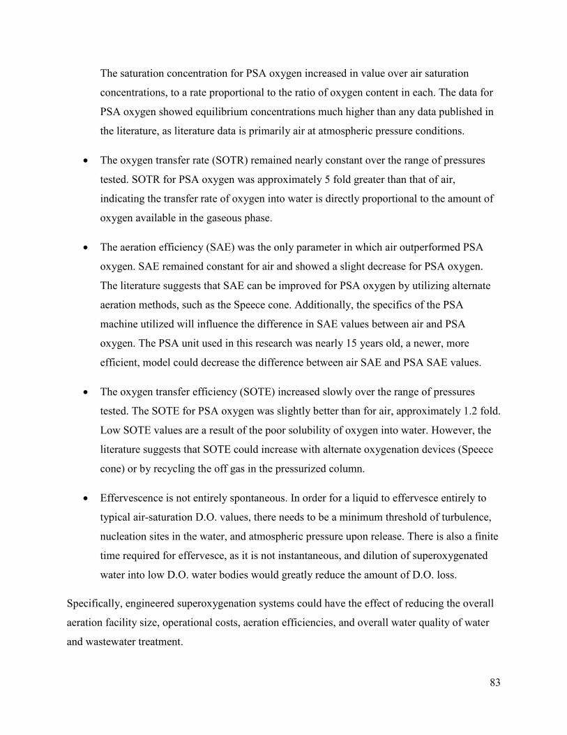
83

The saturation concentration for PSA oxygen increased in value over air saturation

concentrations, to a rate proportional to the ratio of oxygen content in each. The data for

PSA oxygen showed equilibrium concentrations much higher than any data published in

the literature, as literature data is primarily air at atmospheric pressure conditions.

• The oxygen transfer rate (SOTR) remained nearly constant over the range of pressures

tested. SOTR for PSA oxygen was approximately 5 fold greater than that of air,

indicating the transfer rate of oxygen into water is directly proportional to the amount of

oxygen available in the gaseous phase.

• The aeration efficiency (SAE) was the only parameter in which air outperformed PSA

oxygen. SAE remained constant for air and showed a slight decrease for PSA oxygen.

The literature suggests that SAE can be improved for PSA oxygen by utilizing alternate

aeration methods, such as the Speece cone. Additionally, the specifics of the PSA

machine utilized will influence the difference in SAE values between air and PSA

oxygen. The PSA unit used in this research was nearly 15 years old, a newer, more

efficient, model could decrease the difference between air SAE and PSA SAE values.

• The oxygen transfer efficiency (SOTE) increased slowly over the range of pressures

tested. The SOTE for PSA oxygen was slightly better than for air, approximately 1.2 fold.

Low SOTE values are a result of the poor solubility of oxygen into water. However, the

literature suggests that SOTE could increase with alternate oxygenation devices (Speece

cone) or by recycling the off gas in the pressurized column.

• Effervescence is not entirely spontaneous. In order for a liquid to effervesce entirely to

typical air-saturation D.O. values, there needs to be a minimum threshold of turbulence,

nucleation sites in the water, and atmospheric pressure upon release. There is also a finite

time required for effervesce, as it is not instantaneous, and dilution of superoxygenated

water into low D.O. water bodies would greatly reduce the amount of D.O. loss.

Specifically, engineered superoxygenation systems could have the effect of reducing the overall

aeration facility size, operational costs, aeration efficiencies, and overall water quality of water

and wastewater treatment.

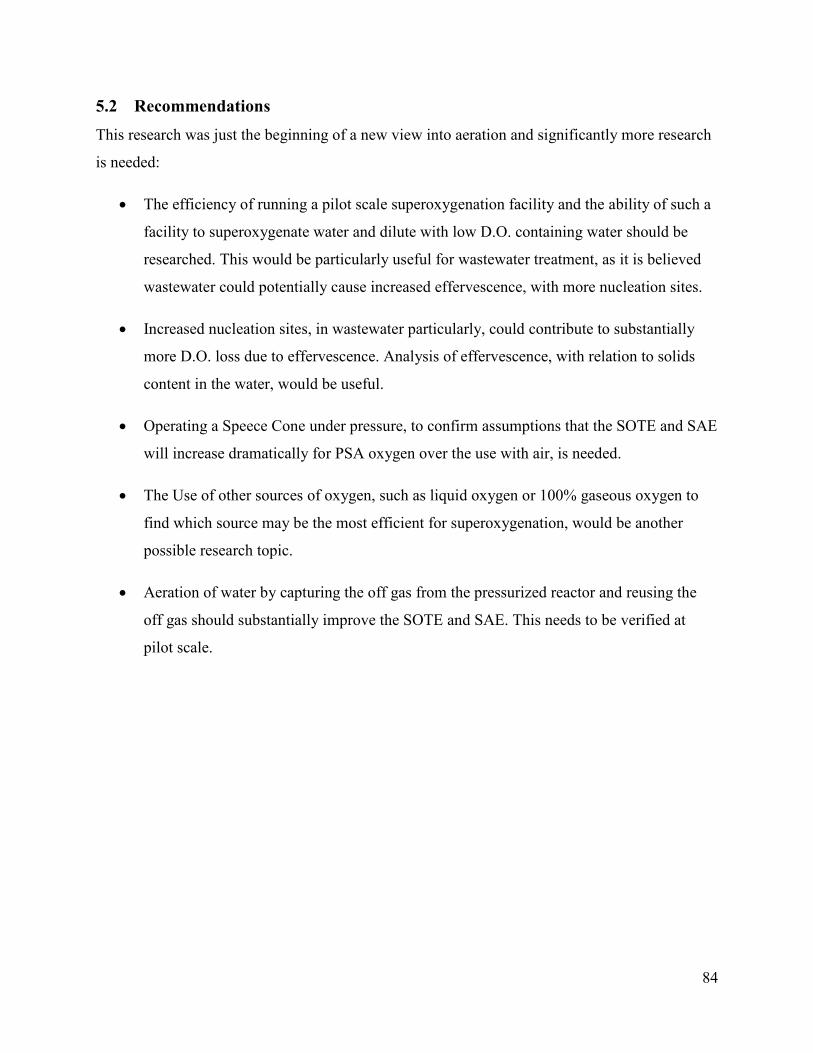
84

5.2 Recommendations

This research was just the beginning of a new view into aeration and significantly more research

is needed:

• The efficiency of running a pilot scale superoxygenation facility and the ability of such a

facility to superoxygenate water and dilute with low D.O. containing water should be

researched. This would be particularly useful for wastewater treatment, as it is believed

wastewater could potentially cause increased effervescence, with more nucleation sites.

• Increased nucleation sites, in wastewater particularly, could contribute to substantially

more D.O. loss due to effervescence. Analysis of effervescence, with relation to solids

content in the water, would be useful.

• Operating a Speece Cone under pressure, to confirm assumptions that the SOTE and SAE

will increase dramatically for PSA oxygen over the use with air, is needed.

• The Use of other sources of oxygen, such as liquid oxygen or 100% gaseous oxygen to

find which source may be the most efficient for superoxygenation, would be another

possible research topic.

• Aeration of water by capturing the off gas from the pressurized reactor and reusing the

off gas should substantially improve the SOTE and SAE. This needs to be verified at

pilot scale.

85

References

AirSep Corporation. (2002). AS-20 - 1000 Instruction Manual. 1:1 – 8:1.

American Water Works Association, American Public Health Association, and Water

Environment Federation. (1992). “Inorganic Nonmetals.” Standard Methods for the

Examination of Water and Wastewater, A. E. Greenberg, L. S. Clesceri, and A. D. Eaton,

eds., American Public Health Association, Washington DC, 4–99:4–102.

ASCE. (2007). Measurement of Oxygen Transfer in Clean Water: ASCE Standard. American

Society of Civil Engineers, Reston, VA, 1–32.

Ashley, K., Fattah, K., Mavinic, D., and Kosari, S. (2014). “Analysis of design factors

influencing the oxygen transfer of a pilot-scale Speece Cone hypolimnetic aerator.” Journal

of Environmental Engineering, ASCE 140(3).

Ashley, K. I. (2002). “Comparative Analysis of Oxygen Transfer in Full Lift and Downflow

Bubble Contact Hypolimnetic Aerators.” Ph.D. Thesis, University of British Columbia.

Ashley, K. I., Mavinic, D. S., and Hall, K. J. (2008). “Oxygenation performance of a laboratory-

scale Speece Cone hypolimnetic aerator: preliminary assessment.” Canadian Journal of

Civil Engineering, 35(7), 663–675.

Ball, J. E., and Humenick, M. J. (1972). “High-Purity Oxygen in Biological Treatment of

Municipal Wastewater.” Water Pollution Control Federation, 44(1), 65–76.

Beak Consultants Ltd. (1977). CPAR Project Report 542-1. State of the art Review: Aeration.

Montreal.

Beutel, M. W. (2003). “Hypolimnetic Anoxia and Sediment Oxygen Demand in California

Drinking Water Reservoirs.” Lake and Reservoir Management, 19(3), 208–221.

Beutel, M. W., and Horne, A. J. (1999). “A Review of the Effects of Hypolimnetic Oxygenation

on Lake and Reservoir Water Quality.” Lake and Reservoir Management, 15(4), 285–297.

Brown, L. C., and Baillod, C. R. (1982). “Modeling and Interpreting Oxygen Transfer Data.”

Journal of the Environmental Engineering Division, 108(4), 607–628.

Caldwell, C., and Hinshaw, J. (1994). “Physiological and haematological responses in rainbow

trout subjected to supplemental dissolved oxygen in fish culture.” Aquaculture, 126, 183–

193.

Colt, J., Sheahan, J. E., and Bouck, G. R. (1993). “Evaluation of the ‘Michigan’ Type Pure

Oxygen Columns for Oxygen Addition and Nitrogen Removal.” Aquaculture Engineering,

12, 141–154.

86

Colt, J., and Watten, B. (1988). “Applications of Pure Oxygen in Fish Culture.” Aquaculture

Engineering, 7, 397–441.

Cooke, G. D., Welch, E. B., Peterson, S. A., and Newroth, P. R. (1993). Restoration and

Management of Lakes and Reservoirs. Lewis Publishers, Boca Raton.

Danckwertz, P. V. (1951). “Significance of Liquid-Film Coefficients in Gas Absorption.”

Industrial and Engineering Chemistry, 43(6), 1460–1467.

Davis, M. L., and Masten, S. J. (2009). Principles of Environmental Engineering and Science.

The McGraw-Hill Companies, New York, 481–495.

Eckenfelder, W. W. (1952). “Aeration Efficiency and Design: I. Measurement of Oxygen

Transfer Efficiency.” Sewage and Industrial Wastes, 24(10), 1221–1228.

Eckenfelder, W. W. (1959). “Absorption of oxygen from air bubbles in water.” Journal of

Sanitary Engineering Division, 85, 89–99.

Fast, A. W., Dorr, V. A., and Rosen, R. J. (1975). “A submerged hypolimnion aerator.” Water

Resources Research, 11(2), 287–293.

Geankoplis, C. J. (2009). Transport Processes and Separation Process Principles. (M. Vincenti,

ed.), Pearson Education, Inc., Upper Saddle River, 46.

Kowsari, S. (2008). “Analysis of Design Factors Influencing the Oxygen Transfer Efficiency of a

Speece Cone Hypolimnetic Aerator.” M.A.Sc. Thesis, University of British Columbia.

Kyle, B. G. (1999). Chemical and Process Thermodynamics. Prentice Hall, Upper Saddle River.

Letzel, H. M., Schouten, J. C., Krishna, R., and van den Bleek, C. M. (1999). “Gas holdup and

mass transfer in bubble column reactors operated at elevated pressure.” Chemical

Engineering Science, 54, 2237–2246.

Lewis, W. K., and Whitman, W. G. (1924). “Principles of Gas Absorption.” Industrial and

Engineering Chemistry, 16(12), 1215–1220.

Mavinic, D. S., and Bewtra, J. K. (1974). “Mass transfer of oxygen in diffused aeration systems.”

Can. J. Civil. Eng., 1, 71–84.

Metro Vancouver. (2012). The Greater Vancouver Water District Quality Control Annual Report

2012: Volume 2 Rev 1. Vancouver, 31.

Moore, B. C., Chen, P.-H., Funk, W. H., and Yonge, D. (1996). “A Model For Predicting Lake

Sediment Oxygen Demand Following Hypolimntetic Aeration.” Water Resources Bulletin,

32(4), 723–731.

87

Nelson, J. K., and Puntenney, J. L. (1983). “Performance Comparison of the Air and High-

Purity-Oxygen Activated Sludge Systems.” Water Pollution Control Federation, 55(4),

336–340.

Nevers, N. de. (2013). Physical and Chemical Equilibrium for Chemical Engineers. John Wiley

& Sons, Hoboken.

OxyGuard. (2013). OxyGuard Dissolved Oxygen Probe Standard Type: User Manual. Farum,

Denmark, 1–7.

Pentair Aquatic Ecosystems. (2013). PT4 Remote Interface Unit: Installation and User Manual.

Coquitlam.

Sartoris, J. J., and Boehmke, J. R. (1987). Limnological effects of artificial aeration at Lake

Cachuma, California. REC–ERC–87–10: 56 pp.

Severson, R. F., Stark, J. L., and Poole, L. M. (1987). Use Of Oxygen To Commercially Rear

Coho Salmon. Papers On The Use Of Supplemental Oxygen To Increase Hatchery Rearing

Capacity In The Pacific Northwest. Portland, 25–34.

Speece, R. E. (1994). “Later thinking solves stratification problems.” Water Quality

International, 3, 12–15.

Speece, R. E. (2007). Superoxygenation: Facts and Myths. 1–15.

Speece, R. E., Madrid, M., and Needham, K. (1971). “Downflow Bubble Contact Aeration.”

Journal of the Sanitary Engineering Division, ASCE, 97(4), 433–441.

Speece, R. E., Siddiqi, R. H., Auburt, R., and DiMond, E. (1976). reservoir discharge

oxygenation demonstration project of Clark Hill lake. Savannah.

Tchobanoglous, G., Burton, F. L., and Stensel, H. D. (2003). Wastewater Engineering:

Treatment and Reuse. McGraw Hill Education.

Thomas, J. A., Funk, W. H., Moore, B. C., and Budd, W. W. (1994). “Short Term Changes In

Newman Lake Following Hypolimnetic Aeration With The Speece Cone.” Lake and

Reservoir Management, 9(1), 111–113.

Versteeg, G. F., Blauwhoff, P. M. M., and Van Swaaij, W. P. M. (1987). “The Effect of

Diffusivity on Transfer in Stirred Vessels. Gas-Liquid Mass Experiments at Atmospheric

and Elevated Pressures.” Chemical Engineering Science, 42(5), 1103–1119.

Wilhelm, E., Battino, R., and Wilcock, R. J. (1977). “Low-Pressure Solubility of Gases in Liquid

Water.” Journal of Chemical Reviews, 77(2), 219–255.

88

Yoshida, F., and Arakawa, S.-I. (1968). “Pressure dependence of liquid phase mass transfer

coefficients.” American Institute of Chemical Engineers, 14(6), 962–963.

89

Appendix 1: Sample D.O. spreadsheet

The following curves depict the measured D.O. concentration compared to the calculated D.O.

concentration by using non-linear regression to solve equation 2.1. Following the curves is the

excel table used to convert the saturation concentration and mass transfer coefficient to standard

conditions.

0

20

40

60

80

100

120

0.000 5.000 10.000 15.000 20.000 25.000 30.000 35.000 40.000

DO

co

nce

ntr

ati

on

(m

g/l

)

Time

Probe 1

Observed concentration Calculated concentration

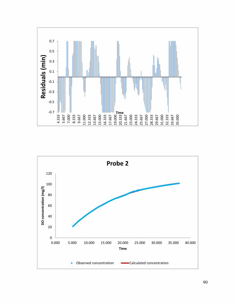
90

-0.7

-0.5

-0.3

-0.1

0.1

0.3

0.5

0.7

4.3

33

5.6

67

7.0

00

8.3

33

9.6

67

11

.00

0

12

.33

3

13

.66

7

15

.00

0

16

.33

3

17

.66

7

19

.00

0

20

.33

3

21

.66

7

23

.00

0

24

.33

3

25

.66

7

27

.00

0

28

.33

3

29

.66

7

31

.00

0

32

.33

3

33

.66

7

35

.00

0

Re

sid

ua

ls (

min

)

Time

0

20

40

60

80

100

120

0.000 5.000 10.000 15.000 20.000 25.000 30.000 35.000 40.000

DO

co

nce

ntr

ati

on

(m

g/l

)

Time

Probe 2


91

-0.7

-0.5

-0.3

-0.1

0.1

0.3

0.5

0.7

5.1

67

6.5

00

7.8

33

9.1

67

10

.50

0

11

.83

3

13

.16

7

14

.50

0

15

.83

3

17

.16

7

18

.50

0

19

.83

3

21

.16

7

22

.50

0

23

.83

3

25

.16

7

26

.50

0

27

.83

3

29

.16

7

30

.50

0

31

.83

3

33

.16

7

34

.50

0

35

.83

3

Re

sid

ua

ls (

min

)

Time

0

20

40

60

80

100

120

0.000 5.000 10.000 15.000 20.000 25.000 30.000 35.000 40.000

DO

co

nce

ntr

ati

on

(m

g/l

)

Time

Probe 3


92

Plant name/Reference and Test Date:

Test 2.0D 3/28/14

Test Conditions

Test Temperature (°C) 19.1

Volume of test tank (m3) 0.241

Volumetric Airflow rate(m3/min) 0.009

Barometric Pressure(in Hg) 100.7

TDS (mg/l) 855

Transfer Parameters (Standard Conditions)

C*∞ 110.66 (mg/l)

Kla (Not TDS corrected) 4.21 (per hour)

Kla (TDS

corrected) 4.2

7 (per

hour)

Co -29.07 (mg/l)

Transfer Parameters (Test Conditions)

C*∞

(mg/L) Kla (per

hour) RMSE (mg/L)

Probe 1 113.58 4.11 0.68

-0.7

-0.5

-0.3

-0.1

0.1

0.3

0.5

0.7

5.8

33

7.1

67

8.5

00

9.8

33

11

.16

7

12

.50

0

13

.83

3

15

.16

7

16

.50

0

17

.83

3

19

.16

7

20

.50

0

21

.83

3

23

.16

7

24

.50

0

25

.83

3

27

.16

7

28

.50

0

29

.83

3

31

.16

7

32

.50

0

33

.83

3

35

.16

7

36

.50

0

Re

sid

ua

ls (

min

)

Time

Probe 2

Probe 3

Probe 4

Probe 5

Probe 6

Site Name/Reference and Test Date:

Test 2.0D 3/28/14

Test Conditions:

Test Temperature

Volume of test tank

Volumetric Airflow rate

Depth of aeration tank

Barometric pressure at site

Input Elevation of site

Barometric pressure at site from elevation

Power input

TDS during test

Properties of Water at test temperature (Program

Weight density

Saturated vapor pressure

Ω (Pressure Correction factors)

τ (Temperature Correction factor)

Values at Test conditions

Probe 2 113.47 3.97 0.43

Probe 3 111.62 4.27 0.92

Probe 4 0.00 0.00

Probe 5 0.00 0.00

Probe 6 0.00 0.00

1 101.325

Site Name/Reference and Test Date:

19.1 °C

0.241 m3

0.009 m3/min

5.46 m

Barometric pressure at site 100.7 kPa

m

Barometric pressure at site from elevation 0 kPa

0.07 kW

855 mg/l

Water at test temperature (Program-calculated)

9.79 kN/m3

2.126 kPa

Ω (Pressure Correction factors) 0.999 0.999

0.994 0.994

τ (Temperature Correction factor) 1.021

Test conditions

Values at Test conditions C

*∞

(mg/L) Kla (per hour)

Probe 1 113.58 4.11

Probe 2 113.47 3.97

Probe 3 111.62 4.27

Probe 4 0.00 0.00

Probe 5 0.00 0.00

Probe 6 0.00 0.00

112.89 4.12

93

0.43

0.92

0.999

0.994

Standard conditions

C*∞

(mg/L) Kla (per hour)

111.33 4.20

111.23 4.06

109.41 4.36

0.00 0.00

0.00 0.00

0.00 0.00

110.66 4.21

94

Average

TDS corrected Kla (standard conditions) 4.27 (per hour)

C*st (Tabulated Saturation DO) 9.258 mg/L

Documents

SUPEROXYGENATION: ANALYSIS OF OXYGEN TRANSFER …