Superintegrability, Exact Solvability, and OrthogonalPolynomials

Sarah Post

Centre de Recherches MathématiquesMontreal, (QC) Canada

NC State University, January 13, 2012

Outline

IntroductionMotivating example: Simple harmonic oscillatorSuperintegrable systems

Second-order superintegrabilityRepresentations of quadratic algebras using Wilson polynomials

Higher-order superintegrable systemsA new superintegrable Hamiltonian with reflectionsA superintegrable system without separation of variables

New results in:

1. E. J. Kalnins, W. Miller Jr. and S. P. Two variable Wilson polynomials andthe generic superintegrable system on the 3-sphere. SIGMA 7, 051(2011) arXiv:1010.3032.

2. S. P., L. Vinet and A. Zhedanov. An infinite family of superintegrableHamiltonians with reflection in the plane. J. Phys. A 44, 505201 (2011)arXiv:1108.5208.

3. S. P. and P. Winterntiz. A nonseparable quantum superintegrable systemin 2D real Euclidean space. J. Phys. A 44, 152001 (2011) arXiv:1101.5405.

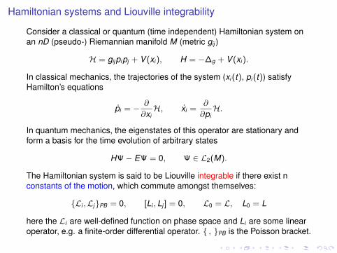
Hamiltonian systems and Liouville integrability

Consider a classical or quantum (time independent) Hamiltonian system onan nD (pseudo-) Riemannian manifold M (metric gij )

H = gijpipj + V (xi ), H = −∆g + V (xi ).

In classical mechanics, the trajectories of the system (xi (t), pi (t)) satisfyHamilton’s equations

pi = − ∂

∂xiH, xi =

∂

∂piH.

In quantum mechanics, the eigenstates of this operator are stationary andform a basis for the time evolution of arbitrary states

HΨ− EΨ = 0, Ψ ∈ L2(M).

The Hamiltonian system is said to be Liouville integrable if there exist nconstants of the motion, which commute amongst themselves:

{Li ,Lj}PB = 0, [Li , Lj ] = 0, L0 = L, L0 = L

here the Li are well-defined function on phase space and Li are some linearoperator, e.g. a finite-order differential operator. { , }PB is the Poisson bracket.

Canonical example

Example (Simple Harmonic Oscillator in 2D)The Hamiltonian for the SHO is given by

H = −∂2x − ∂2

y + ω2(x2 + y2).

It is immediately obvious that this is Hamiltonian is radially symmetric, that is,it admits the first-order integral of the motion

X = y∂x − x∂y , [H,X ] = 0.

The Schrödinger equation for the SHO in polar coordinates haseigenfunctions as

HΦ = EΦ, E = −2ω(2m + n + 1) Φ = cm,n(ωr 2)n2 eωr2/2Ln

m(ωr 2)einθ.

This exact-solvablity is not the case for all group-invariant potentials. the SHOis also superintegrable:

L = −∂2x + ω2x2

This constant of the motion is not associated with group symmetry, butinstead separation of variable in cartesian coordinates.

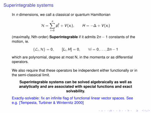
Superintegrable systems

In n dimensions, we call a classical or quantum Hamiltonian

H =nX

i=0

p2i + V (xi ), H = −∆ + V (xi )

(maximally, Nth-order) Superintegrable if it admits 2n − 1 constants of themotion, ie.

{Li ,H} = 0, [Li ,H] = 0, ∀i = 0, . . . , 2n − 1

which are polynomial, degree at most N, in the momenta or as differentialoperators.

We also require that these operators be independent either functionally or inthe semi-classical limit.

Superintegrable systems can be solved algebraically as well asanalytically and are associated with special functions and exact

solvability.

Exactly-solvable: fix an infinite flag of functional linear vector spaces. Seee.g. [Tempesta, Turbiner & Winternitz 2000]

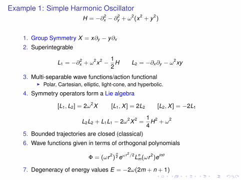
Example 1: Simple Harmonic OscillatorH = −∂2

x − ∂2y + ω2(x2 + y2)

1. Group Symmetry X = x∂y − y∂x

2. Superintegrable

L1 = −∂2x + ω2x2 − 1

2H L2 = −∂x∂y − ω2xy

3. Multi-separable wave functions/action functionalI Polar, Cartesian, elliptic, light-cone, and hyperbolic.

4. Symmetry operators form a Lie algebra

[L1, L2] = 2ω2X [L1,X ] = 2L2 [L2,X ] = −2L1

L2L2 + L1L1 − 2ω2X 2 =14

H2 + ω2

5. Bounded trajectories are closed (classical)

6. Wave functions given in terms of orthogonal polynomials

Φ = (ωr 2)n2 eωr2/2Ln

m(ωr 2)einθ

7. Degeneracy of energy values E = −2ω(2m + n + 1)

Example 2: Smorodinsky-Wintenitz iH = −∂2

x − ∂2y + ω2(x2 + y2)−

14 − a2

x2 −14 − b2

y2 .

1. Group Symmetry

2. Superintegrable

L1 = ∂2x +

1/4− a2

x2 −ω2x2, L2 = (x∂y−y∂x )2+(1/4− a2)y2

x2 +(1/4− b2)x2

y2 .

3. Multi-separable wave functions/action functionalI Polar, Cartesian, elliptic, light-cone, and hyperbolic .

4. Symmetry operators form a quadratic algebra R ≡ [L1, L2]

[R, L1] = 8L21 − 8HL1 + 16ω2L2 − 8ω2,

[R, L2] = 8HL2 − 8{L1, L2}+ (12− 16a2)H + (16a2 + 16b2 − 24)L1.

5. Bounded trajectories are closed (classical)

6. Wave functions given in terms of orthogonal polynomials (quantum)

Φ = cosa−1/2 θ sinb−1/2 θ(ωr 2)n2 eωr2/2L2n+a+b+1

m (ωr 2)Pa,bn (− cos(2θ))

7. Degeneracy of energy values E = −2ω(2m + 2n + a + b + 1)

Classification of Second-order Superintegrable Systems

I Begun with Smorodinsky, Winternitz and collaborators (∼ 1965) studyingsystems which are multi-separable. Gave classification in 2D and 3D onreal Euclidean space.

I Kalnins, Kress, Miller and Pogosyan published a series of papers (∼2000) classifying second-order superintegrable systems on conformallyflat space.

I In 2D, all second-order superintegrable systems are equivalent tosystems on either E(2,C) or S2(C).

I Bijection between classical and quantum systems and potentials dependlinearly on at most 4 constants.

I The wave functions are exactly-solvable in terms of a gauge function andorthogonal polynomials (OPs)

I The algebra of integrals of the motion closes at 6th order and isalgebraically generated by H, L1 L2 and R ≡ [L1, L2].

Models of the quadratic algebras

Just as the representation theory of Lie algebras is associated with the SHO,we can use the representation theory of the quadratic algebras to gain insightinto the physical systems.

1. Look for (finite dimensional) irreducible representations throughrealizations in terms of differential or difference operators and specialfunctions.

2. To date, have given an irreducible representation for each equivalenceclass of second-order superintegrable systems in 2D in terms of functionspace realization. See e.g. SP SIGMA 7 (2011)

3. Special functions/OP which arise: Jacobi polynomials, Laguerrepolynomials, Bessel functions, Dual Hahn polynomials, and Wilsonpolynomials.

4. All such quadratic algebras were realized in terms of differentialoperators except the one associated with the generic superintegrablesystem ∗ on the 2 sphere. The operators defining this algebra arerelated to the Wilson polynomials in full generality.

∗-generic in the sense that all other second-order superintegrable systemscan be obtained through appropriately chose limits (delicate).

The 2D SystemFor n = 2 define the generic sphere system by embedding of S2

x21 + x2

2 + x23 = 1 in three dimensional flat space. The Hamiltonian operator is

H =X

1≤i<j≤3

(xi∂j − xj∂i )2 +

3Xk=1

ak

x2k, ∂i ≡ ∂xi .

The 3 operators that generate the symmetries are L12, L13, L23 where

Lij = (xi∂j − xj∂i )2 +

aix2j

x2i

+ajx2

i

x2j

1 ≤ i < j ≤ 3,

H =X

1≤i<j≤3

Lij +4X

k=1

ak .

These integrals of motion for a quadratic algebra with R = [L23, L13] and

εijk [Ljk ,R] = 4{Ljk , Lij} − 4{Ljk , Lik} − (8 + 16aj )Lik + (8 + 16ak )Lij + 8(aj − ak ),

R2 =83{L23, L13, L12} − (16a1 + 12)L2

23 − (16a2 + 12)L213 − (16a3 + 12)L2

12

+523

({L23, L13}+ {L13, L12}+ {L12, L23}) +13

(16 + 176a1)L23 +13

(16 + 176a2)L13

+13

(16 + 176a3)L12 +323

(a1 + a2 + a3) + 48(a1a2 + a2a3 + a3a1) + 64a1a2a3.

Here εijk is the pure skew-symmetric tensor, and {A,B} = AB + BA with ananalogous definition of {A,B,C} as a symmetrized sum of 6 terms.

The Wilson Polynomials

Before we proceed to the model, we us present a basic overview of some ofthe characteristics of the Wilson polynomials [ Wilson 1980]

wn(t2) ≡ wn(t2, α, β, γ, δ) = (α + β)n(α + γ)n(α + δ)n×

4F3

„−n, α + β + γ + δ + n − 1, α− t , α + tα + β, α + γ, α + δ

; 1«

= (α + β)n(α + γ)n(α + δ)nΦ(α,β,γ,δ)n (t2).

The polynomial wn(t2) is symmetric in α, β, γ, δ.The Wilson polynomials are eigenfunctions of a divided difference operatorgiven as

τ∗τΦn = n(n + α + β + γ + δ − 1)Φn

whereEAF (t) = F (t + A), τ =

12t

(E1/2 − E−1/2),

τ∗ =12t

h(α + t)(β + t)(γ + t)(δ + t)E1/2 − (α− t)(β − t)(γ − t)(δ − t)E−1/2

i.

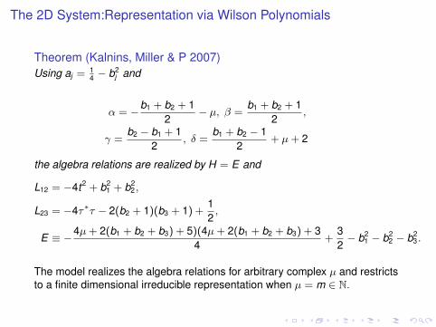
The 2D System:Representation via Wilson Polynomials

Theorem (Kalnins, Miller & P 2007)Using aj = 1

4 − b2j and

α = −b1 + b2 + 12

− µ, β =b1 + b2 + 1

2,

γ =b2 − b1 + 1

2, δ =

b1 + b2 − 12

+ µ+ 2

the algebra relations are realized by H = E and

L12 = −4t2 + b21 + b2

2,

L23 = −4τ∗τ − 2(b2 + 1)(b3 + 1) +12,

E ≡ −4µ+ 2(b1 + b2 + b3) + 5)(4µ+ 2(b1 + b2 + b3) + 34

+32− b2

1 − b22 − b2

3.

The model realizes the algebra relations for arbitrary complex µ and restrictsto a finite dimensional irreducible representation when µ = m ∈ N.

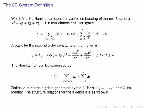
The 3D System:Definition

We define the Hamiltonian operator via the embedding of the unit 3-spherex2

1 + x22 + x2

3 + x24 = 1 in four dimensional flat space.

H =X

1≤i<j≤4

(xi∂j − xj∂i )2 +

4Xk=1

ak

x2k, ∂i ≡ ∂xi .

A basis for the second order constants of the motion is

Lij ≡ Lji = (xi∂j − xj∂i )2 +

aix2j

x2i

+ajx2

i

x2j, 1 ≤ i < j ≤ 4.

The Hamiltonian can be expressed as

H =X

1≤i<j≤4

Lij +4X

k=1

ak .

Define A to be the algebra generated by the Lij for all i, j = 1, .., 4 and I, theidentity. The structure relations for the algebra are as follows:

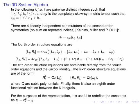
The 3D System:AlgebraIn the following i, j, k , ` are pairwise distinct integers such that1 ≤ i, j, k , ` ≤ 4, and εijk is the completely skew-symmetric tensor such thatεijk = 1 if i < j < k .

There are 4 linearly independent commutators of the second ordersymmetries (no sum on repeated indices) [Kalnins, Miller and P. 2011]:

R` = εijk [Lij , Ljk ]

The fourth order structure equations are

[Lij ,Rj ] = 4εi`k ({Lik , Lj`} − {Li`, Ljk}+ Li` − Lik + Ljk − Lj`)

[Lij ,Rk ] = 4εij`({Lij , Li` − Lj`}+ (2 + 4aj )Li` − (2 + 4ai )Lj` + 2ai − 2aj ).

The fifth order structure equations are obtainable directly from the fourthorder equations and the Jacobi identity. The sixth order structure equationsare of the form

R2` = Q`(Lij ), {Ri ,Rj} = Qij (Lij ),

where Q are cubic polynomials. Finally, there is also an eighth orderfunctional relation between the 6 integrals.

For the purposes of the representation, it is useful to redefine the constantsas ai = b2

i − 14 .

Subalgebras

We note that the algebra described above contains several copies of2-sphere algebra. Then, we can see that there exist subalgebras Ak

generated by the set {Lij , I} for i, j 6= k and that these algebras are exactlythose associated to the 2D analog of this system. Furthermore, if we define

Hk ≡X

i<j,i,j 6=k

Lij − (Xj 6=k

b2i −

34

)I

then Hk will commute with all the elements of Ak and will represent theHamiltonian for the associated system.

For example, A4 ⊂ A the algebra generated by L12, L13, L23 and the identity, Ihas as it center

H4 = L12 + L13 + L23 + (3/4− b21 − b2

2 − b23)I

which is the Hamiltonian for the associated 2-sphere system in coordinatesx2

1 + x22 + x2

3 = 1..

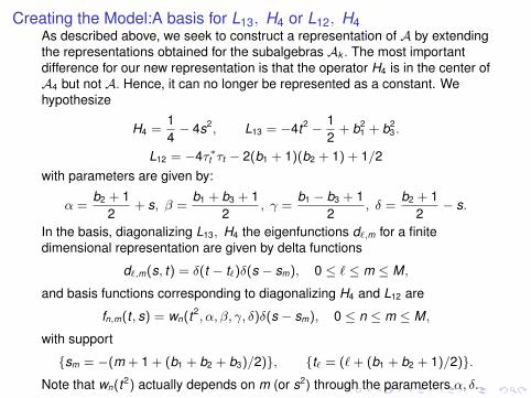
Creating the Model:A basis for L13, H4 or L12, H4As described above, we seek to construct a representation of A by extendingthe representations obtained for the subalgebras Ak . The most importantdifference for our new representation is that the operator H4 is in the center ofA4 but not A. Hence, it can no longer be represented as a constant. Wehypothesize

H4 =14− 4s2, L13 = −4t2 − 1

2+ b2

1 + b23.

L12 = −4τ∗t τt − 2(b1 + 1)(b2 + 1) + 1/2with parameters are given by:

α =b2 + 1

2+ s, β =

b1 + b3 + 12

, γ =b1 − b3 + 1

2, δ =

b2 + 12− s.

In the basis, diagonalizing L13, H4 the eigenfunctions d`,m for a finitedimensional representation are given by delta functions

d`,m(s, t) = δ(t − t`)δ(s − sm), 0 ≤ ` ≤ m ≤ M,

and basis functions corresponding to diagonalizing H4 and L12 are

fn,m(t , s) = wn(t2, α, β, γ, δ)δ(s − sm), 0 ≤ n ≤ m ≤ M,

with support

{sm = −(m + 1 + (b1 + b2 + b3)/2)}, {t` = (`+ (b1 + b2 + 1)/2)}.

Note that wn(t2) actually depends on m (or s2) through the parameters α, δ.

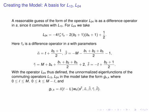
Creating the Model: A basis for L13,L24

A reasonable guess of the form of the operator L24 is as a difference operatorin s, since it commutes with L13. For L24 we take

L24 = −4τ∗s τs − 2(b2 + 1)(b4 + 1) +12.

Here τs is a difference operator in s with parameters

α = t +b2 + 1

2, β = −M − b1 + b2 + b3

2− 1,

γ = M + b4 +b1 + b2 + b3

2+ 2, δ = −t +

b2 + 12

.

With the operator L24 thus defined, the unnormalized eigenfunctions of thecommuting operators L13, L24 in the model take the form gn,k where0 ≤ ` ≤ M, 0 ≤ k ≤ M − `, and

g`,k = δ(t − t`)wk (s2, α, β, γ, δ).

To complete the model, we will need parameter dependent raising andlowering operators for the Wilson polynomials,

R =1

2y[T 1/2 − T−1/2].

RΦn =n(n + α + β + γ + δ − 1)

(α + β)(α + γ)(α + δ)Φ

(α+1/2,β+1/2,γ+1/2,δ+1/2)n−1 .

L =1

2y

h(α− 1/2 + y)(β − 1/2 + y)(γ − 1/2 + y)(δ − 1/2 + y)T 1/2

−(α− 1/2− y)(β − 1/2− y)(γ − 1/2− y)(δ − 1/2− y)T−1/2i.

LΦn = (α + β − 1)(α + γ − 1)(α + δ − 1)Φ(α−1/2,β−1/2,γ−1/2,δ−1/2)n+1 .

Lαβ =1

2y

h−(α− 1/2 + y)(β − 1/2 + y)T 1/2 + (α− 1/2− y)(β − 1/2− y)T−1/2

i.

LαβΦn = −(α + β − 1)Φ(α−1/2,β−1/2,γ+1/2,δ+1/2)n .

We finalize the construction of our model by realizing the operator L34. Theoperator L34 must commute with L12, so we hypothesize that it is of the form

L34 = A(s)S(LαβLαγ)t + B(s)S−1(LγδLβδ)t + C(s)(LR)t + D(s).

Since the eigenfunctions for L12 are

fn,m(t , s) = wn(t2, α, β, γ, δ)δ(s − sm).

On the other hand, we can consider the action of L34 on the basis g`,k :

g`,k = δ(t − t`)wk (s2, α, β, γ, δ).

Considering L34 primarily as an operator on s we hypothesize that it must beof the form

L34 = A(t)T (LαβLαγ)s + B(t)T−1(LγδLβδ)s + C(t)(LR)s

+D(t)s2 + E(t) + κL12.

By a long and tedious computation we can verify that the 3rd order structureequations are satisfied for certain choices of functions. We also obtain thequantization for E , for finite dimensional representations,

E = −(2M +4X

j=1

bj + 3)2)− 1.

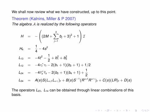
We shall now review what we have constructed, up to this point.

Theorem (Kalnins, Miller & P 2007)The algebra A is realized by the following operators

H = −

0@(2M +4X

j=1

bj + 3)2 + 1

1A IH4 =

14− 4s2

L13 = −4t2 − 12

+ b21 + b2

3

L12 = −4τ∗t τt − 2(b1 + 1)(b2 + 1) + 1/2

L24 = −4τ∗s τs − 2(b2 + 1)(b4 + 1) +12

L34 = A(s)S(LαβLαγ)t + B(s)S−1(RαβRαγ)t + C(s)(LR)t + D(s)

The operators L23, L14 can be obtained through linear combinations of thisbasis.

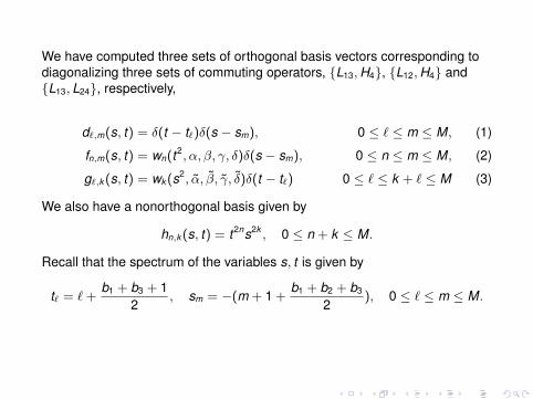
We have computed three sets of orthogonal basis vectors corresponding todiagonalizing three sets of commuting operators, {L13,H4}, {L12,H4} and{L13, L24}, respectively,

d`,m(s, t) = δ(t − t`)δ(s − sm), 0 ≤ ` ≤ m ≤ M, (1)

fn,m(s, t) = wn(t2, α, β, γ, δ)δ(s − sm), 0 ≤ n ≤ m ≤ M, (2)

g`,k (s, t) = wk (s2, α, β, γ, δ)δ(t − t`) 0 ≤ ` ≤ k + ` ≤ M (3)

We also have a nonorthogonal basis given by

hn,k (s, t) = t2ns2k , 0 ≤ n + k ≤ M.

Recall that the spectrum of the variables s, t is given by

t` = `+b1 + b3 + 1

2, sm = −(m + 1 +

b1 + b2 + b3

2), 0 ≤ ` ≤ m ≤ M.

Relation with Tratnik’s polynomials

It is possible to write an inner product on the finite dimensional representationas

〈f (t , s), g(t , s)〉 =

Z Zf (t , s)g(t , s)ω(t , s)δ(t − t`)δ(s − sm)dsdt ,

with

ω(t`, sm) =M!(1 + b4)M−m(M + b1 + b2 + b3 + b4 + 3)m(2m + 2 + b1 + b2 + b3)

(M − m)!(1 + b4)M (M + b1 + b2 + b3 + 3)m(2 + b1 + b2 + b3)

×(1 + b1)`(1 + b1 + b3)`(1 + b2)m−`(2 + b1 + b2 + b3)m+`(2` + 1 + b1 + b3)

`!(m − `)!(1 + b3)`(2 + b1 + b3)m+`(1 + b1 + b3)c20,0

This is exactly the weight function for an n-variable generalization of theWilson polynomials given by Tratnik 1991.

Further, it can be seen by direct computation that the operators which arediagonalized by the Tratnik polynomials [Geronimo & Iliev 2010] can bewritten in terms of the operators L12 and L14 + L12 + L24 and so form a basisfor the representation of A.

Conclusion 1

I Introduce the "generic" superintegrable system on the n-sphere.I The representation theory of the 2-d system can be constructed in terms

of Wilson polynomials.I The representation theory of the 3-d system can be constructed in terms

of a two variable generalization of the Wilson polynomials introduced byTratnik.

I These representations give information about the original system, i.e.eigenvalues of symmetry operators and inter-basis expansioncoefficients.

I The algebra gives the structure of recurrence operators which act on theWilson polynomials.

I For the future:I Study the system on the n-sphere: n − 1 variable Tratnik polynomials.I Consider limiting processes on the system to get other representations in

terms of orthogonal polynomials-in analogy with Askey-Wilson tableau.I q-analogs?

Example 3: Tremblay, Turbiner & Winternitz

H = ∂2r +

1r∂r +

1r 2 ∂

2θ − ω2r 2 +

( 14 − a2)k2

r 2 cos2 kθ+

( 14 − b2)k2

r 2 sin2 kθ.

1. Group Symmetry

2. Superintegrable for rational k = p/q [Kalnins, Kress, Miller & Pogosyan2011]

∃L1, L2 = ∂2r +

( 14 − a2)k2

cos2 kθ+

( 14 − b2)k2

sin2 kθ.

3. Multi- separable wave functions/action functionalI Polar, Cartesian, elliptic, light-cone, and hyperbolic .

4. Symmetry operators form a polynomial algebra

5. Bounded trajectories are closed (classical)

6. Wave functions given in terms of orthogonal polynomials (quantum)

Φ = c1 cosa−1/2 θ sinb−1/2 θ(ωr 2)n2 eωr2/2Lpn/q+a+b+1

m (ωr 2)Pa,bn

„− cos(2

pqθ)

«7. Degeneracy of energy values E = −2ω(2m + 2p

q n + a + b + 1)

Why (higher-order) Superintegrability?

It may be intuitively obvious why we would care about second-ordersuperintegrability because of its connection to multiseparability. Less obviousperhaps is the uses of the higher-order integral.

Answer: Special Functions and exact solvability

Many of the special functions of mathematical physics are associated withsuperintegrable systems and perhaps the key to their tractability lies in thehigher-order integrals and polynomial algebras which give recurrencerelations for the special functions.

Conversely, it is possible to use known recurrence relations for specialfunctions to construct integrals of motion for superintegrable systems whichadmit separation of variables. Miller, Kalnins Kress 2011 proved thesuperintegrability of the TTW system using recurrence relations for Jacobiand Laguerre polynomials.

The little -1 Jacobi polynomialsThe set of classical orthogonal polynomials can be extended to includepolynomial eigenfunctions of first-order differential operators of Dunkl-type.[Vinet & Zhedanov 2011]

The simplest of these heretofore "missing" classical orthogonal polynomialsare called little −1 Jacobi polynomials and satisfy

Λ ≡»2(1− x)

ddx

R +“α + β + 1− α

x

”(1− R)

–,

ΛP(α,β)n (x) = λn,α,βP(α,β)

n (x), Rf (x) = f (−x)

where

λn,α,β =

−2n for n even,

2(n + α + β + 1) for n odd.

These polynomials can be expressed in terms of the hypergeometric(terminating) series. As their name indicates, they can be obtained as aq → −1 limit of the little q-Jacobi polynomials. For α > −1, β > −1, they areorthogonal over the interval [−1, 1] with respect to the weight function

ω(x) = |x |α(1− x2)(β+1)/2(1 + x).

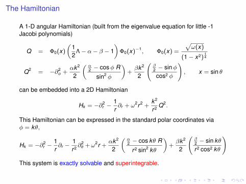
The Hamiltonian

A 1-D angular Hamiltonian (built from the eigenvalue equation for little -1Jacobi polynomials)

Q = Φ0(x)

„12

Λ− α− β − 1«

Φ0(x)−1, Φ0(x) =

pω(x)

(1− x2)14

Q2 = −∂2φ +

αk2

2

„ α2 − cosφ R

sin2 φ

«+βk2

2

β2 − sinφcos2 φ

!, x = sin θ

can be embedded into a 2D Hamiltonian

Hk = −∂2r −

1r∂r + ω2r 2 +

k2

r 2 Q2.

This Hamiltonian can be expressed in the standard polar coordinates viaφ = kθ,

Hk = −∂2r −

1r∂r −

1r 2 ∂

2θ +ω2r +

αk2

2

„ α2 − cos kθ R

r 2 sin2 kθ

«+βk2

2

β2 − sin kθr 2 cos2 kθ

!

This system is exactly solvable and superintegrable.

The wave functions

The eigenfunctions for the Schrödinger equation admit separation of variables

Ψ(r , φ) = R(r)Φ(φ).

„−∂2

r −1r∂r −

A2

r 2 + ω2r 2«

R(r) = ER(r).

withQ2Φ(φ) = a2

nΦ(φ), A = k |an|.

If the energy is restricted to

Em,n = 2ω[2m + k |an|+ 1], an =

−n − α+β+1

2 n evenn + α+β+1

2 n odd

The components of the wave function are

R(r) = Y Am(r) = Km (

√ωr)Ae−ω

2r2/2LAm(ωr 2)

Φ(φ) = Xn(φ) =Nn

N0Φ0(φ)P(α,β)

n (sinφ).

Raising and lowering operators

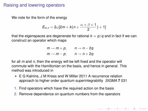
We note for the form of the energy

Em,n = 2ω[2m + k(n +α + β + 1

2) + 1]

that the eigenspaces are degenerate for rational k = p/q and in fact if we canconstruct an operator which maps

m→ m + p, n→ n − 2q

m→ m − p, n→ n + 2q

for all m and n, then the energy will be left fixed and the operator willcommute with the Hamiltonian on the basis, and hence in general. Thismethod was introduced in

I E G Kalnins, J M Kress and W Miller 2011 A recurrence relationapproach to higher order quantum superintegrability SIGMA 7 031

1. Find operators which have the required action on the basis

2. Remove dependence on quantum numbers from the operators

Raising and Lowering operators for Φ(φ)

First, we need to raise or lower n by 2q. To do this, we have the operators J+

and J− which are parameter independent

J+ = (x + (x − 1)R)

„Q − 1

2

«+ α + β

J− = (x + (1− x)R)

„Q +

12

«− α + β

and which have the following action

J+Pn =

(2n(α+β+n)(α+β+2n)

Pn−1 n even−2(α + β + 2n + 2)Pn+1 n odd

J−Pn =

(2(α + β + 2n + 2)Pn+1 n even− 2(α+n)(β+n)

(α+β+2n)Pn−1 n odd .

The operator which will change the degree of Xn by 2 is given by

Φ0J−J+Φ−10 Xn =

(− 4n(α+β+n)(α−1+n)(β−1+n)

(α+β+2n)(α+β+2n−2)Xn−2 n even

−4(α + β + 2n + 2)(α + β + 2n + 4)Xn+2 n odd .

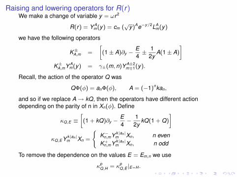
Raising and lowering operators for R(r)We make a change of variable y = ωr 2

R(r) = Y Am(y) = cm (

√y)Ae−y/2LA

m(y)

we have the following operators

K±A,m =

»(1± A)∂y −

E4± 1

2yA(1± A)

–K±A,mY A

m(y) = γ±(m, n)Y A±2m∓1(y).

Recall, the action of the operator Q was

QΦ(φ) = anΦ(φ), A = (−1)nkan,

and so if we replace A→ kQ, then the operators have different actiondepending on the parity of n in Xn(φ). Define

κQ,E ≡»

(1 + kQ)∂y −E4− 1

2ykQ(1 + Q)

–κQ,E Y k|an|

m Xn =

(K−n,mY k|an|

m Xn, n evenK +

n,mY k|an|m Xn, n odd

To remove the dependence on the values E = Em,n we use

κpQ,H = κp

Q,E |E=H .

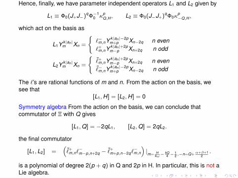
Hence, finally, we have parameter independent operators L1 and L2 given by

L1 ≡ Φ0(J+J−)qΦ−10 κp

Q,H , L2 ≡ Φ0(J−J+)qΦ0κp−Q,H ,

which act on the basis as

L1Y k|an|m Xn =

(`−m,nY k|an|−2p

m+p Xn−2q n even`+m,nY k|an|+2p

m−p Xn+2q n odd

L2Y k|an|m Xn =

(˜+m,nY k|an|+2p

m−p Xn+2q n even˜−m,nY k|an|−2p

m+p Xn−2q n odd

The `’s are rational functions of m and n. From the action on the basis, wesee that

[L1,H] = [L2,H] = 0

Symmetry algebra From the action on the basis, we can conclude thatcommutator of Ξ with Q gives

[L1,Q] = −2qL1, [L2,Q] = 2qL2.

the final commutator

[L1, L2] =“

˜+m,n`

−m−p,n+2q − ˜+

m+p,n−2q`−m,n

”|m= H

4ω−kQ4 −

12 ,−n=Q+α+β+1

2.

is a polynomial of degree 2(p + q) in Q and 2p in H. In particular, this is not aLie algebra.

Conclusions 2

I We have shown how the new little -1 Jacobi polynomials can be use as abasis of eigenfunctions for a superintegrable Hamiltonian withreflections.

I We have used the raising and lowering operators for the little -1 Jacobipolynomials, in conjunction with those of the Laguerre polynomials toprove the superintegrability of the 2D Hamiltonian.

Future perspectivesI Construct other systems using known raising/lowering operators for

OPs.1. Extending other separable Hamiltonians by "adding k’s" (with P. Winternitz

and D. Levesque)2. To other, non-classical OPs, e.g. exceptional OPs (with S. Tsujimoto and L.

Vinet)

I Use superintegrable systems to find raising/lowering/recurrencerelations for OPs.

Non-separable superintegrable systems

What remains if we have non-separable superintegrability?

1. Group Symmetry

2. Multi- separable wave functions/action functional

3. All integrals of motion of degree N > 2

4. Degeneracy of energy values

5. Bounded trajectories are closed (classical)

6. Symmetry operators form a polynomial algebra ???

7. Wave functions given in terms of orthogonal polynomials (quantum)???

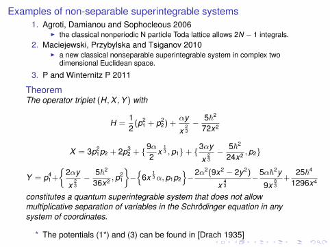
Examples of non-separable superintegrable systems1. Agroti, Damianou and Sophocleous 2006

I the classical nonperiodic N particle Toda lattice allows 2N − 1 integrals.2. Maciejewski, Przybylska and Tsiganov 2010

I a new classical nonseparable superintegrable system in complex twodimensional Euclidean space.

3. P and Winternitz P 2011

TheoremThe operator triplet (H,X ,Y ) with

H =12

(p21 + p2

2) +αy

x23− 5~2

72x2

X = 3p21p2 + 2p3

2 + {9α2

x13 , p1}+ {3αy

x23− 5~2

24x2 , p2}

Y = p41+

2αy

x23− 5~2

36x2 , p21

ff−n

6x13α, p1p2

o−2α2(9x2 − 2y2)

x43

−5α~2y

9x83

+25~4

1296x4

constitutes a quantum superintegrable system that does not allowmultiplicative separation of variables in the Schrödinger equation in anysystem of coordinates.

* The potentials (1*) and (3) can be found in [Drach 1935]

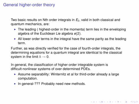
General higher-order theory

Two basic results on Nth order integrals in E2, valid in both classical andquantum mechanics, are:

I The leading ( highest-order in the momenta) term lies in the envelopingalgebra of the Euclidean Lie algebra e(2).

I All lower order terms in the integral have the same parity as the leadingterm.

Further, as was directly verified for the case of fourth-order integrals, thedetermining equations for a quantum integral are identical to the classicalsystem in the limit ~→ 0.

In general, the classification of higher-order integrable system isdifficult-nonlinear systems of over determined PDEs.

I Assume separability: Winternitz et al for third-order already a largecomputation.

I In general-??? Probably need new methods.

Conclusions 3

I We have seen how higher-order superintegrable systems retain many ofthe properties of second-order superintegrable systems and evensystems which admit a group symmetry.

I We have demonstrated a new non-separable, quantum superintegrablesystem with non-trivial classical limit.

I We have shown the general results for Nth-order integrals in N = 4 case,i.e. parity of terms, highest order terms are in enveloping algebra of e(2).

There are many open problems in this area. It remains to be seen, fornon-separable superintegrable systems

I If the higher-order integrals can be used to solve for the wave functions,(exactly solvable?)

I If the wave functions are related to know special functions or, if they arenew, if they admit special function-like properties

I If the Hamiltonians can be written in algebraic form in terms of thegenerators of a hidden/dynamical symmetry algebra

I If the Lie symmetries of the system (e.g. of the equations of motion) canbe used.

I Can we see the structure of superintegrability in scattering states?

Thank you for your attention

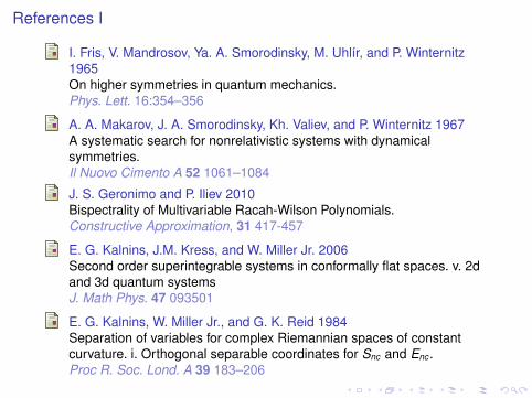
References I

I. Fris, V. Mandrosov, Ya. A. Smorodinsky, M. Uhlír, and P. Winternitz1965On higher symmetries in quantum mechanics.Phys. Lett. 16:354–356

A. A. Makarov, J. A. Smorodinsky, Kh. Valiev, and P. Winternitz 1967A systematic search for nonrelativistic systems with dynamicalsymmetries.Il Nuovo Cimento A 52 1061–1084

J. S. Geronimo and P. Iliev 2010Bispectrality of Multivariable Racah-Wilson Polynomials.Constructive Approximation, 31 417-457

E. G. Kalnins, J.M. Kress, and W. Miller Jr. 2006Second order superintegrable systems in conformally flat spaces. v. 2dand 3d quantum systemsJ. Math Phys. 47 093501

E. G. Kalnins, W. Miller Jr., and G. K. Reid 1984Separation of variables for complex Riemannian spaces of constantcurvature. i. Orthogonal separable coordinates for Snc and Enc .Proc R. Soc. Lond. A 39 183–206

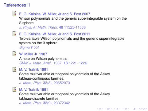
References II

E. G. Kalnins, W. Miller, Jr and S. Post 2007Wilson polynomials and the generic superintegrable system on the2-sphereJ. Phys. A: Math. Theor. 40 11525-11538

E. G. Kalnins, W. Miller, Jr and S. Post 2011Two-variable Wilson polynomials and the generic superintegrablesystem on the 3-sphereSigma 7 051

W. Miller Jr. 1987A note on Wilson polynomialsSIAM J. Math. Anal., 1987, 18 1221–1226

M. V. Tratnik 1991Some multivariable orthogonal polynomials of the Askeytableau-continuous families.J. Math. Phys. 32(8), 20652073

M. V. Tratnik 1991Some multivariable orthogonal polynomials of the Askeytableau-discrete families.J. Math. Phys. 32(9), 23372342

References III

Tremblay F, Turbiner A V and Winternitz P 2009An infinite family of solvable and integrable quantum systems on theplaneJ. Phys. A 42 242001

Vinet L and Zhedanov A 2011A "missing" family of classical orthogonal polynomialsJ. Phys. A 44 085201

J. Wilson 1980Some hypergeometric orthogonal polynomialsSIAM J. Math. Anal. 11 690–701