Embed Size (px)
Citation preview

Super Tips
and Tricks

Content
Super Tips & Tricks Content......................................................................... 1 Content .................................................................................................. 2
Part I: Super Excel Tips and Tricks............................................3 About This Handbook .................................................................................. 4
Part II: Manipulating Data in Access .....................................9

Super Tips and Tricks • Page 3
Part I: Super Excel Tips
and Tricks

Super Tips and Tricks • Page 4
About This Handbook
This handbook was created by Angela Bolick with the assistance of Eric Lawson and Kelvin Testado as reference material for users who will view and print reports. It will be used during the Super Tips and Tricks class. The handbook is divided into two sections:
• Part I Super Excel Tips and Tricks
• Part II Manipulating Data in Access
Names used in the documentation are fictitious.
Super Tips and Tricks • Page 5
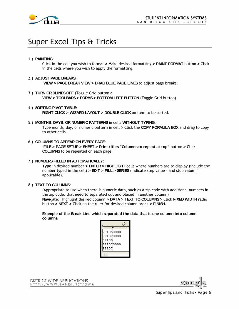
Super Excel Tips & Tricks
1.) PAINTING: Click in the cell you wish to format > Make desired formatting > PAINT FORMAT button > Click in the cells where you wish to apply the formatting.
2.) ADJUST PAGE BREAKS:
VIEW > PAGE BREAK VIEW > DRAG BLUE PAGE LINES to adjust page breaks.
3.) TURN GRIDLINES OFF (Toggle Grid button): VIEW > TOOLBARS > FORMS > BOTTOM LEFT BUTTON (Toggle Grid button).
4.) SORTING PIVOT TABLE:
RIGHT CLICK > WIZARD LAYOUT > DOUBLE CLICK on item to be sorted.
5.) MONTHS, DAYS, OR NUMERIC PATTERNS in cells WITHOUT TYPING: Type month, day, or numeric pattern in cell > Click the COPY FORMULA BOX and drag to copy to other cells.
6.) COLUMNS TO APPEAR ON EVERY PAGE:
FILE > PAGE SETUP > SHEET > Print titles “Columns to repeat at top” button > Click COLUMNS to be repeated on each page.
7.) NUMBERS FILLED IN AUTOMATICALLY:
Type in desired number > ENTER > HIGHLIGHT cells where numbers are to display (include the number typed in the cell) > EDIT > FILL > SERIES (indicate step value – and stop value if applicable).
8.) TEXT TO COLUMNS:
(Appropriate to use when there is numeric data, such as a zip code with additional numbers in the zip code, that need to separated out and placed in another column) Navigate: Highlight desired column > DATA > TEXT TO COLUMNS > Click FIXED WIDTH radio button > NEXT > Click on the ruler for desired column break > FINISH. Example of the Break Line which separated the data that is one column into column columns.
Super Tips and Tricks • Page 6
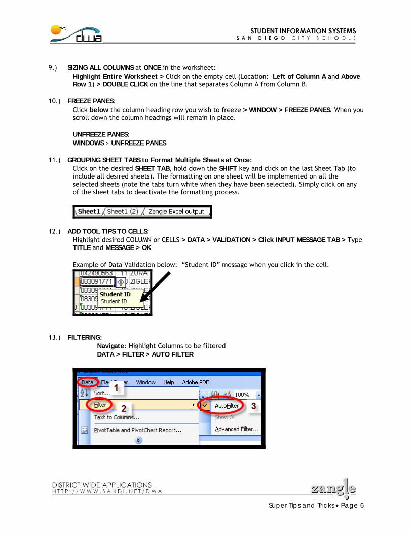
9.) SIZING ALL COLUMNS at ONCE in the worksheet:
Highlight Entire Worksheet > Click on the empty cell (Location: Left of Column A and Above Row 1) > DOUBLE CLICK on the line that separates Column A from Column B.
10.) FREEZE PANES: Click below the column heading row you wish to freeze > WINDOW > FREEZE PANES. When you scroll down the column headings will remain in place. UNFREEZE PANES: WINDOWS > UNFREEZE PANES
11.) GROUPING SHEET TABS to Format Multiple Sheets at Once: Click on the desired SHEET TAB, hold down the SHIFT key and click on the last Sheet Tab (to include all desired sheets). The formatting on one sheet will be implemented on all the selected sheets (note the tabs turn white when they have been selected). Simply click on any of the sheet tabs to deactivate the formatting process.
12.) ADD TOOL TIPS TO CELLS: Highlight desired COLUMN or CELLS > DATA > VALIDATION > Click INPUT MESSAGE TAB > Type TITLE and MESSAGE > OK Example of Data Validation below: “Student ID” message when you click in the cell.
13.) FILTERING: Navigate: Highlight Columns to be filtered
DATA > FILTER > AUTO FILTER
Super Tips and Tricks • Page 7
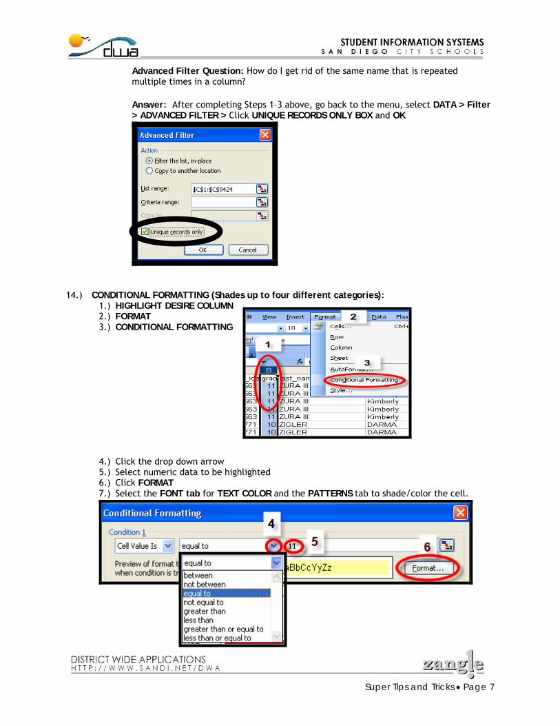
Advanced Filter Question: How do I get rid of the same name that is repeated multiple times in a column?
Answer: After completing Steps 1–3 above, go back to the menu, select DATA > Filter > ADVANCED FILTER > Click UNIQUE RECORDS ONLY BOX and OK
14.) CONDITIONAL FORMATTING (Shades up to four different categories): 1.) HIGHLIGHT DESIRE COLUMN 2.) FORMAT 3.) CONDITIONAL FORMATTING
4.) Click the drop down arrow 5.) Select numeric data to be highlighted 6.) Click FORMAT 7.) Select the FONT tab for TEXT COLOR and the PATTERNS tab to shade/color the cell.
Super Tips and Tricks • Page 8
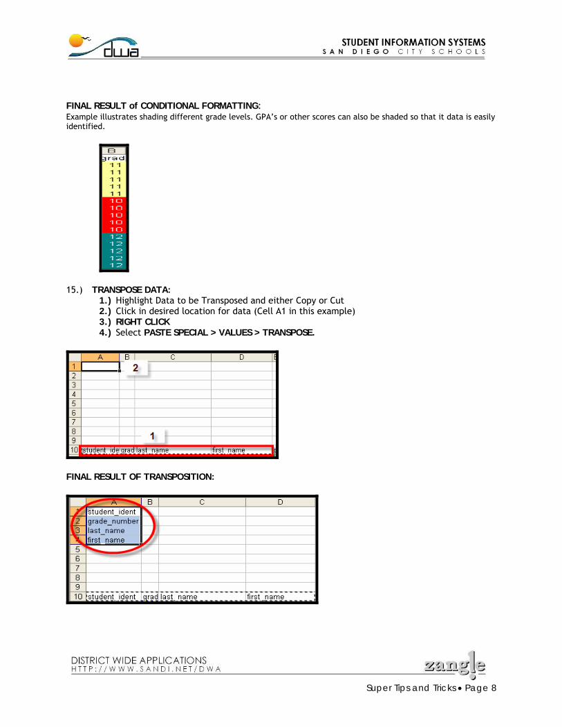
FINAL RESULT of CONDITIONAL FORMATTING: Example illustrates shading different grade levels. GPA’s or other scores can also be shaded so that it data is easily identified.
15.) TRANSPOSE DATA:
1.) Highlight Data to be Transposed and either Copy or Cut 2.) Click in desired location for data (Cell A1 in this example) 3.) RIGHT CLICK 4.) Select PASTE SPECIAL > VALUES > TRANSPOSE.
FINAL RESULT OF TRANSPOSITION:

Super Tips and Tricks • Page 9
Part II: Manipulating Data
in Access
Super Tips and Tricks • Page 10
Manipulating Data in Access
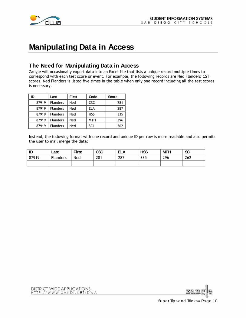
The Need for Manipulating Data in Access Zangle will occasionally export data into an Excel file that lists a unique record multiple times to correspond with each test score or event. For example, the following records are Ned Flanders' CST scores. Ned Flanders is listed five times in the table when only one record including all the test scores is necessary. ID Last First Code Score
87919 Flanders Ned CSC 281
87919 Flanders Ned ELA 287
87919 Flanders Ned HSS 335
87919 Flanders Ned MTH 296
87919 Flanders Ned SCI 262
Instead, the following format with one record and unique ID per row is more readable and also permits the user to mail merge the data: ID Last First CSC ELA HSS MTH SCI 87919 Flanders Ned 281 287 335 296 262

Super Tips and Tricks • Page 11
Step 1: Plan Ahead
Make a list of the fields you want in your final report. Then search the existing views in Zangle to determine which reports contain the necessary fields. Make sure you identify a common unique field in each report. This field will help link the reports together later on. The most common unique field is the student ID.
Super Tips and Tricks • Page 12
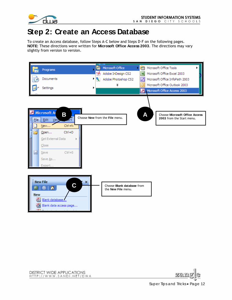
Step 2: Create an Access Database To create an Access database, follow Steps A-C below and Steps D–F on the following pages. NOTE: These directions were written for Microsoft Office Access 2003. The directions may vary slightly from version to version.
Choose Microsoft Office Access 2003 from the Start menu.
A Choose New from the File menu.
Choose Blank database from the New File menu.
C
B
Super Tips and Tricks • Page 13
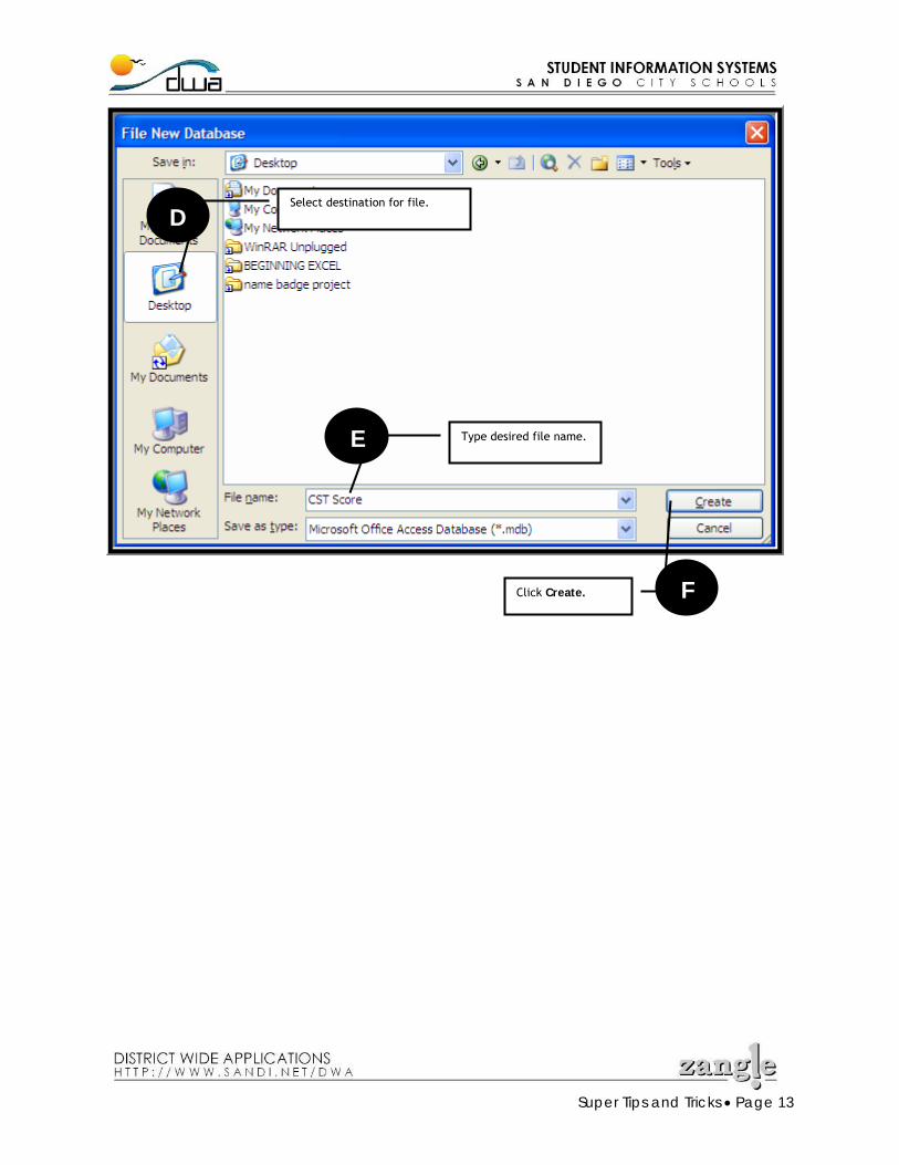
E
F
D Select destination for file.
Click Create.
Type desired file name.
Super Tips and Tricks • Page 14
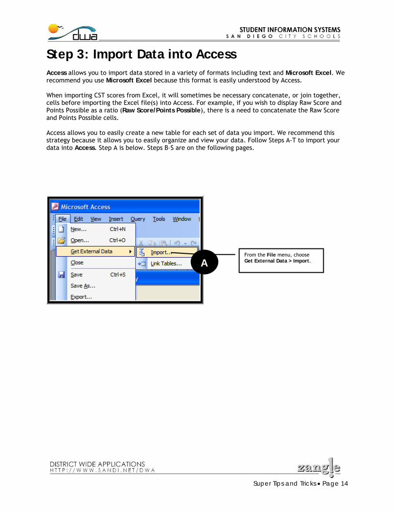
Step 3: Import Data into Access Access allows you to import data stored in a variety of formats including text and Microsoft Excel. We recommend you use Microsoft Excel because this format is easily understood by Access. When importing CST scores from Excel, it will sometimes be necessary concatenate, or join together, cells before importing the Excel file(s) into Access. For example, if you wish to display Raw Score and Points Possible as a ratio (Raw Score/Points Possible), there is a need to concatenate the Raw Score and Points Possible cells. Access allows you to easily create a new table for each set of data you import. We recommend this strategy because it allows you to easily organize and view your data. Follow Steps A-T to import your data into Access. Step A is below. Steps B–S are on the following pages.
From the File menu, choose Get External Data > Import. A
Super Tips and Tricks • Page 15
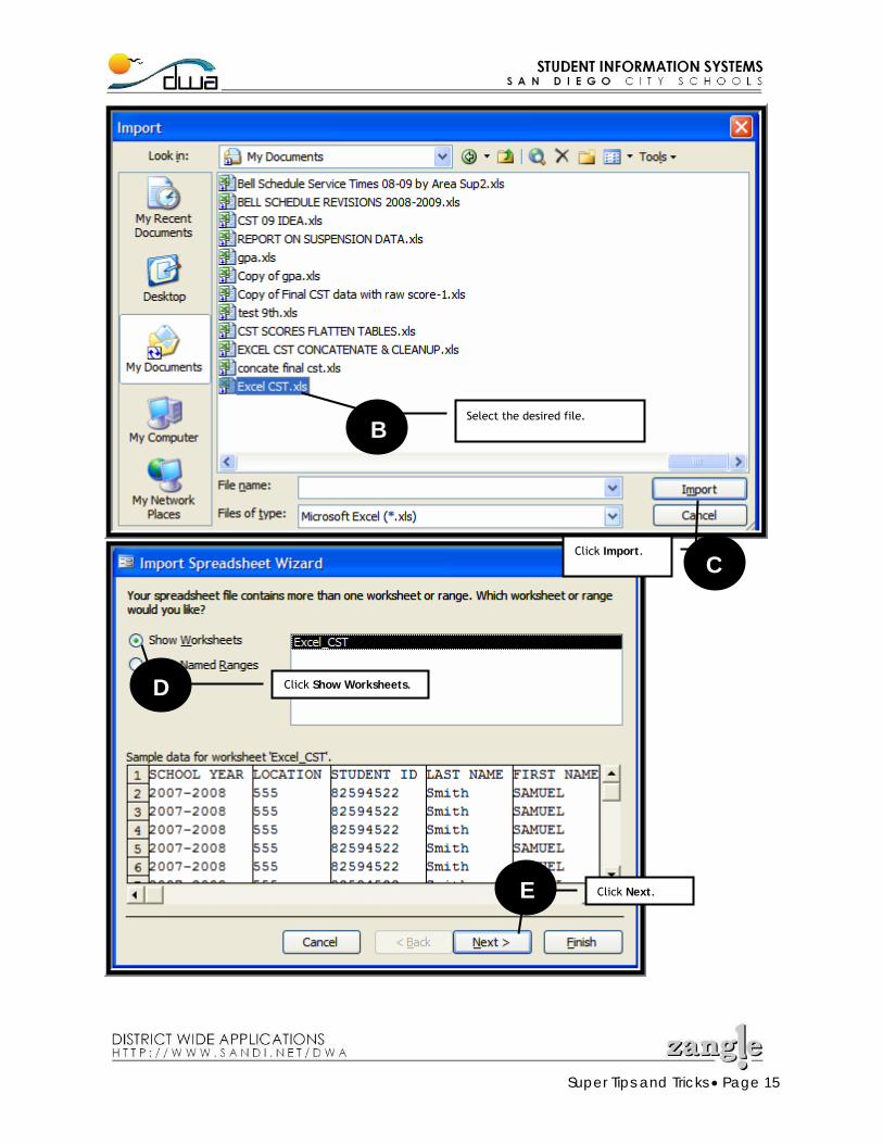
Click Import.
Select the desired file.
C
B
Click Show Worksheets.
Click Next.
D
E
Super Tips and Tricks • Page 16
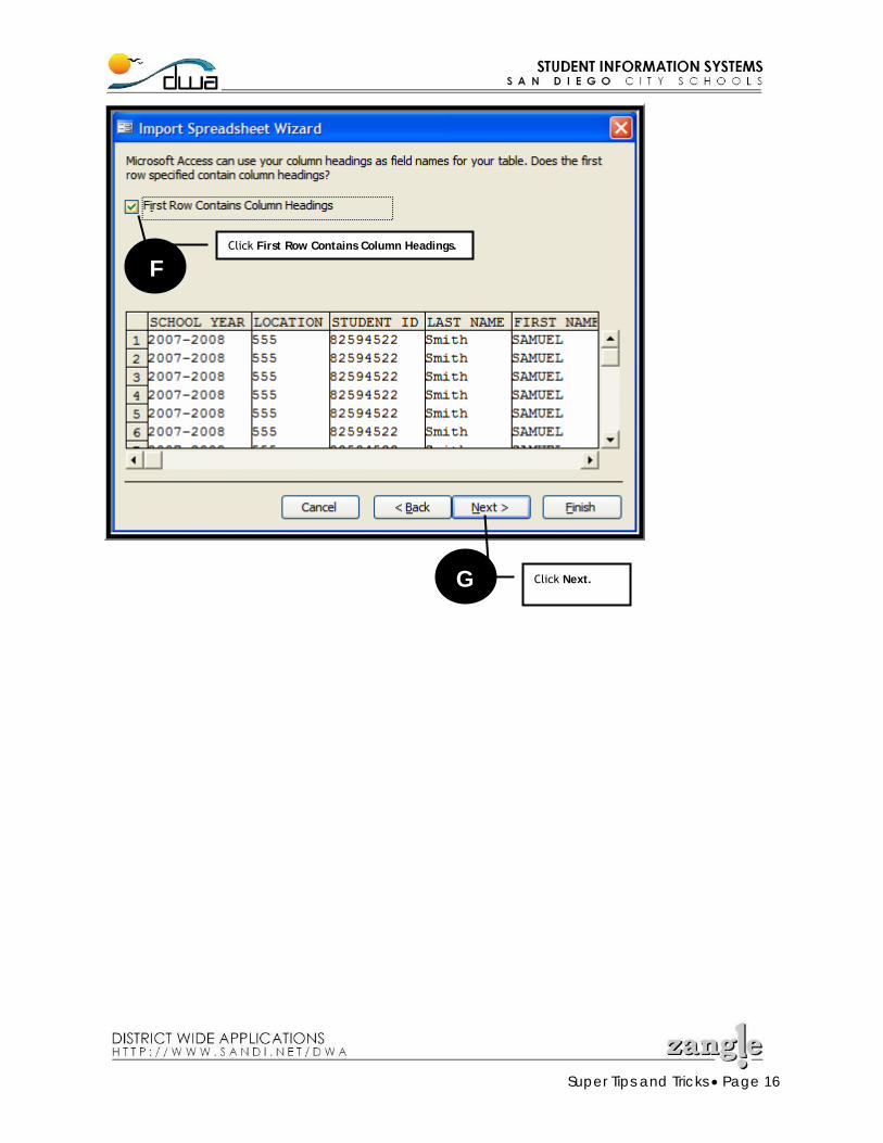
F Click First Row Contains Column Headings.
Click Next. G
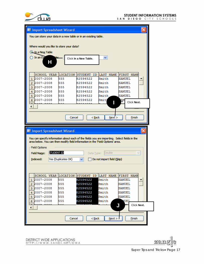
Super Tips and Tricks • Page 17
I
H
Click Next.
Click In a New Table.
Click Next. J
Super Tips and Tricks • Page 18
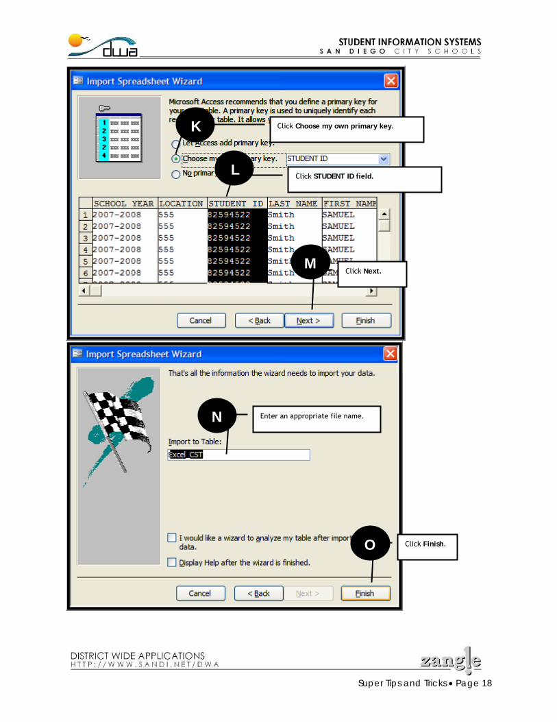
Click Choose my own primary key. K
Click Next. M
Enter an appropriate file name. N
Click Finish. O
Click STUDENT ID field. L
Super Tips and Tricks • Page 19
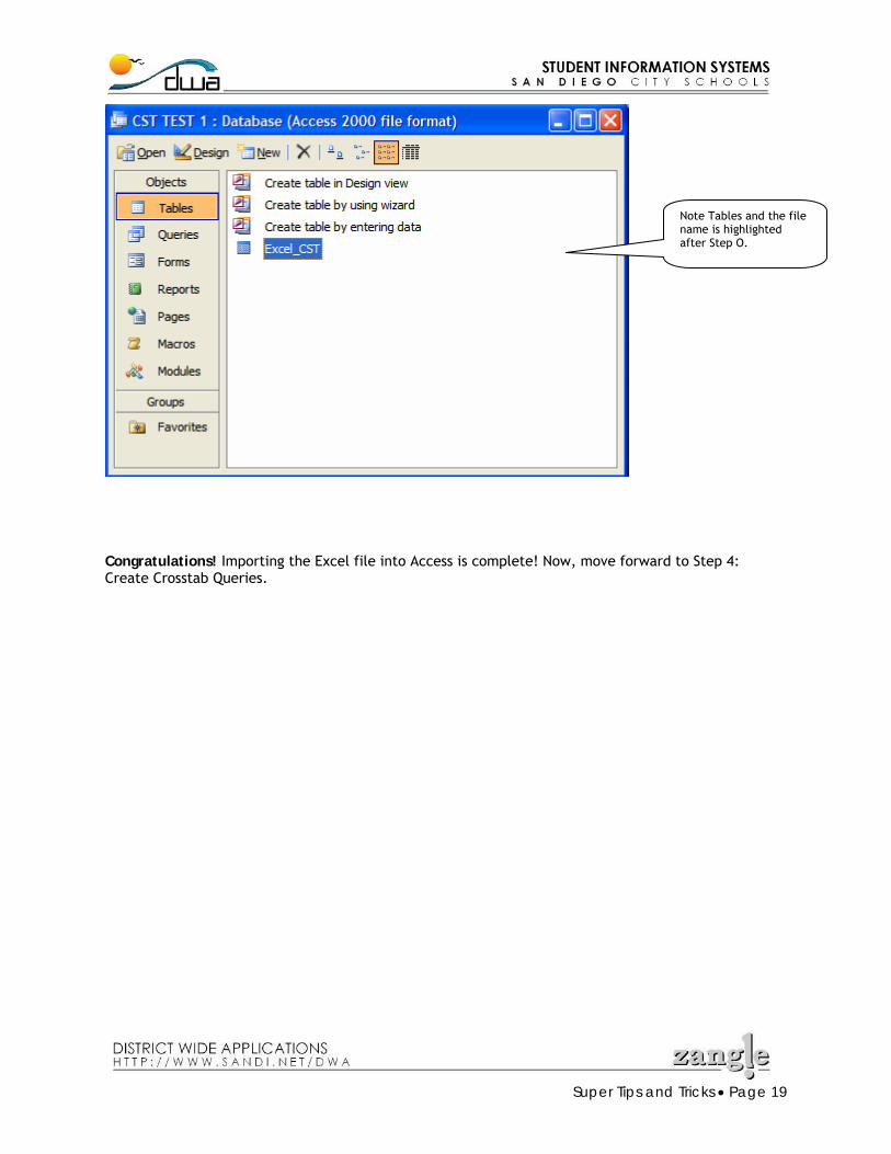
Congratulations! Importing the Excel file into Access is complete! Now, move forward to Step 4: Create Crosstab Queries.
Note Tables and the file name is highlighted after Step O.
Super Tips and Tricks • Page 20
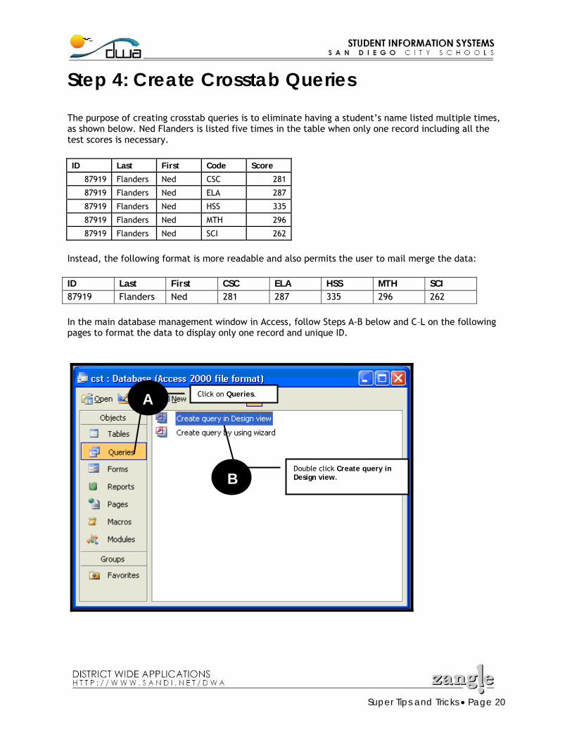
Step 4: Create Crosstab Queries
The purpose of creating crosstab queries is to eliminate having a student’s name listed multiple times, as shown below. Ned Flanders is listed five times in the table when only one record including all the test scores is necessary. ID Last First Code Score
87919 Flanders Ned CSC 281
87919 Flanders Ned ELA 287
87919 Flanders Ned HSS 335
87919 Flanders Ned MTH 296
87919 Flanders Ned SCI 262
Instead, the following format is more readable and also permits the user to mail merge the data: ID Last First CSC ELA HSS MTH SCI 87919 Flanders Ned 281 287 335 296 262 In the main database management window in Access, follow Steps A-B below and C–L on the following pages to format the data to display only one record and unique ID.
Click on Queries. A
Double click Create query in Design view. B
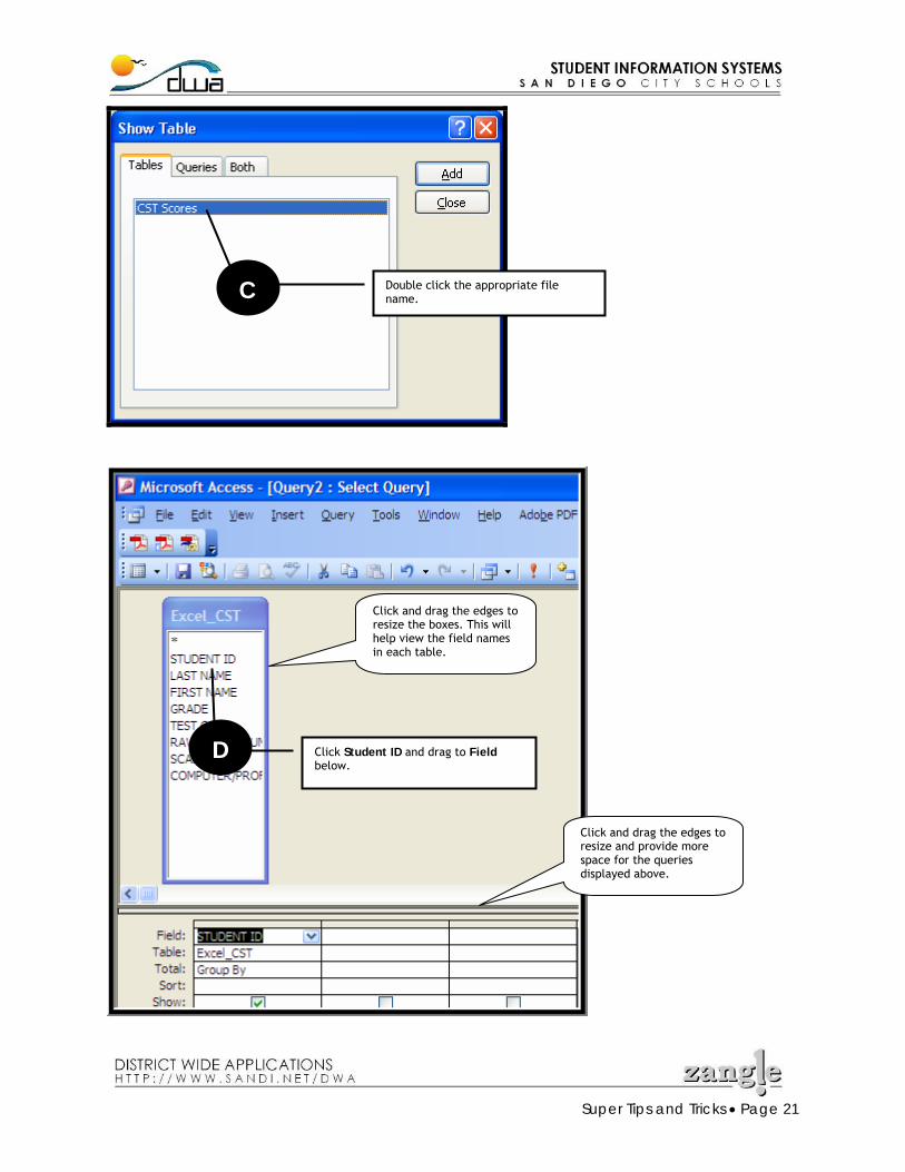
Super Tips and Tricks • Page 21
Double click the appropriate file name.
C
Click Student ID and drag to Field below.
D
Click and drag the edges to resize the boxes. This will help view the field names in each table.
Click and drag the edges to resize and provide more space for the queries displayed above.
Super Tips and Tricks • Page 22
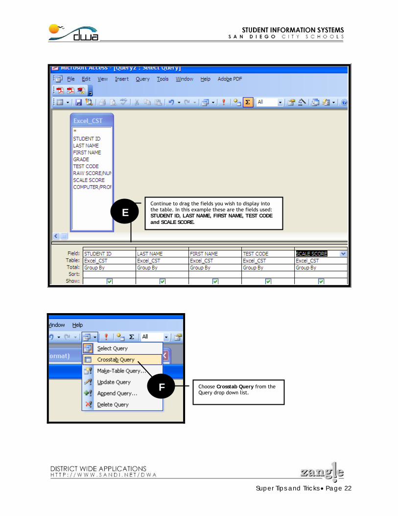
Choose Crosstab Query from the Query drop down list.
F
Continue to drag the fields you wish to display into the table. In this example these are the fields used: STUDENT ID, LAST NAME, FIRST NAME, TEST CODE and SCALE SCORE.
E
Super Tips and Tricks • Page 23
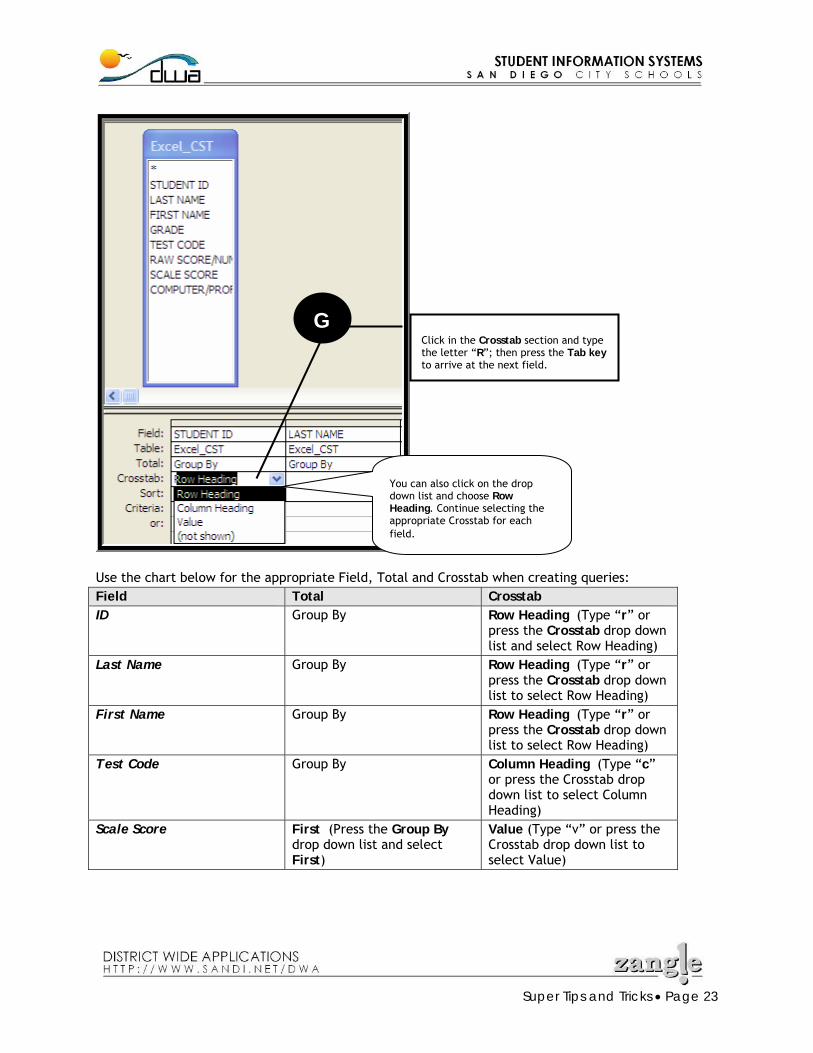
Use the chart below for the appropriate Field, Total and Crosstab when creating queries: Field Total Crosstab ID Group By Row Heading (Type “r” or
press the Crosstab drop down list and select Row Heading)
Last Name Group By Row Heading (Type “r” or press the Crosstab drop down list to select Row Heading)
First Name Group By Row Heading (Type “r” or press the Crosstab drop down list to select Row Heading)
Test Code Group By Column Heading (Type “c” or press the Crosstab drop down list to select Column Heading)
Scale Score First (Press the Group By drop down list and select First)
Value (Type “v” or press the Crosstab drop down list to select Value)
Click in the Crosstab section and type the letter “R”; then press the Tab key to arrive at the next field.
G
You can also click on the drop down list and choose Row Heading. Continue selecting the appropriate Crosstab for each field.
Super Tips and Tricks • Page 24
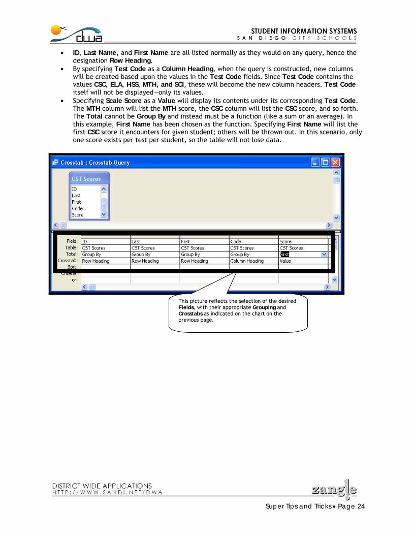
• ID, Last Name, and First Name are all listed normally as they would on any query, hence the designation Row Heading.
• By specifying Test Code as a Column Heading, when the query is constructed, new columns will be created based upon the values in the Test Code fields. Since Test Code contains the values CSC, ELA, HSS, MTH, and SCI, these will become the new column headers. Test Code itself will not be displayed―only its values.
• Specifying Scale Score as a Value will display its contents under its corresponding Test Code. The MTH column will list the MTH score, the CSC column will list the CSC score, and so forth. The Total cannot be Group By and instead must be a function (like a sum or an average). In this example, First Name has been chosen as the function. Specifying First Name will list the first CSC score it encounters for given student; others will be thrown out. In this scenario, only one score exists per test per student, so the table will not lose data.
This picture reflects the selection of the desired Fields, with their appropriate Grouping and Crosstabs as indicated on the chart on the previous page.
Super Tips and Tricks • Page 25
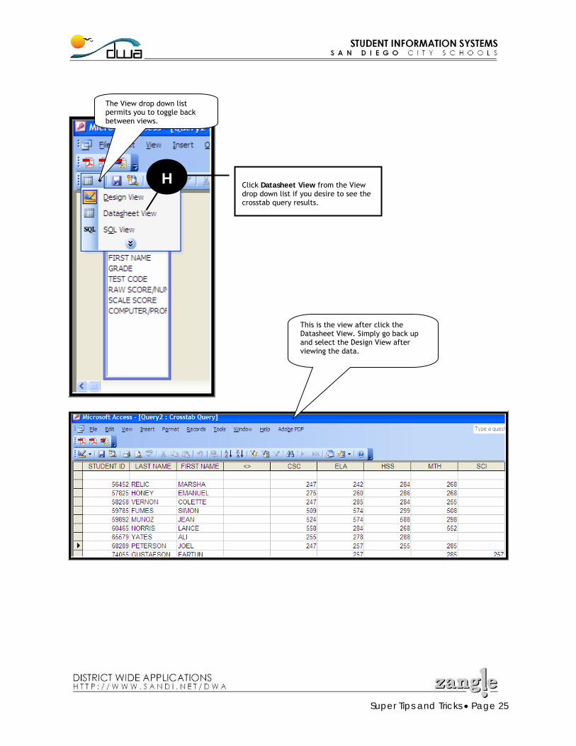
Click Datasheet View from the View drop down list if you desire to see the crosstab query results.
H
The View drop down list permits you to toggle back between views.
This is the view after click the Datasheet View. Simply go back up and select the Design View after viewing the data.
Super Tips and Tricks • Page 26
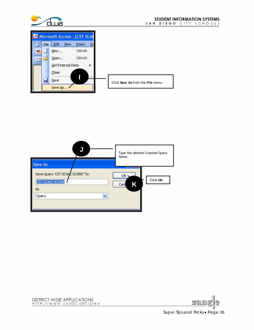
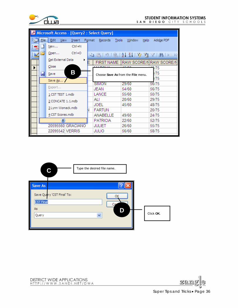
Click Save As from the File menu.
I
Type the desired Crosstab Query Name.
J
Click OK.
K
Super Tips and Tricks • Page 27
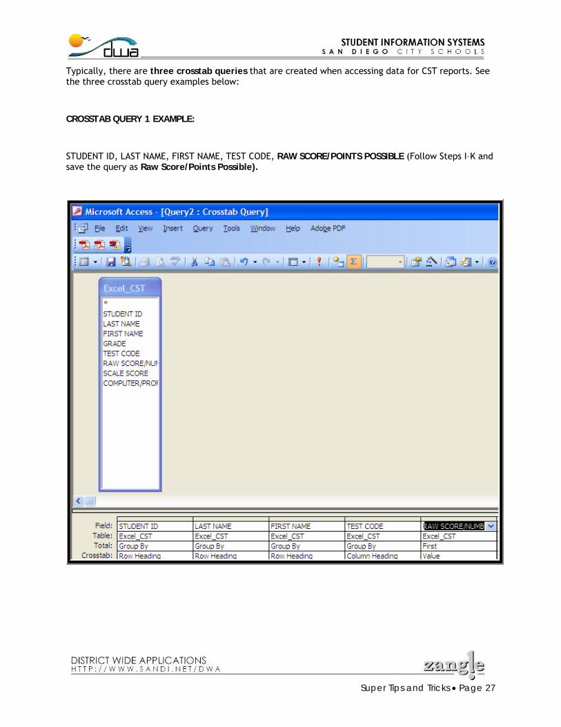
Typically, there are three crosstab queries that are created when accessing data for CST reports. See the three crosstab query examples below:
CROSSTAB QUERY 1 EXAMPLE:
STUDENT ID, LAST NAME, FIRST NAME, TEST CODE, RAW SCORE/POINTS POSSIBLE (Follow Steps I–K and save the query as Raw Score/Points Possible).
Super Tips and Tricks • Page 28
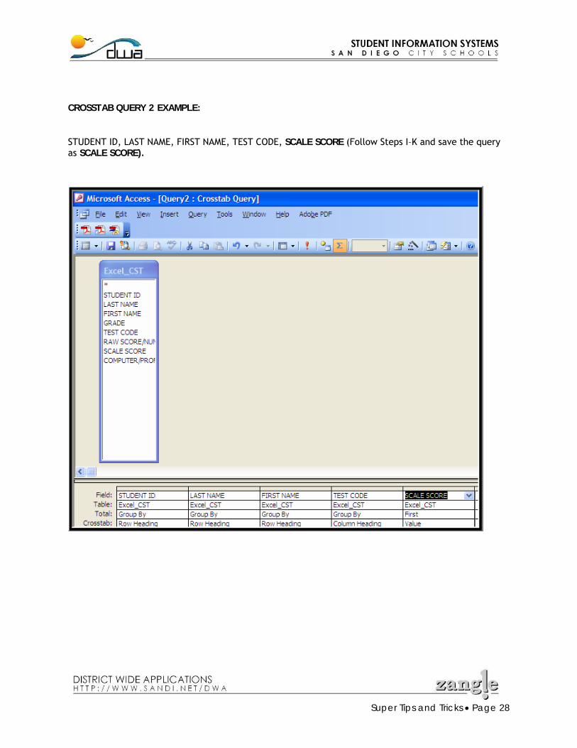
CROSSTAB QUERY 2 EXAMPLE: STUDENT ID, LAST NAME, FIRST NAME, TEST CODE, SCALE SCORE (Follow Steps I–K and save the query as SCALE SCORE).
Super Tips and Tricks • Page 29
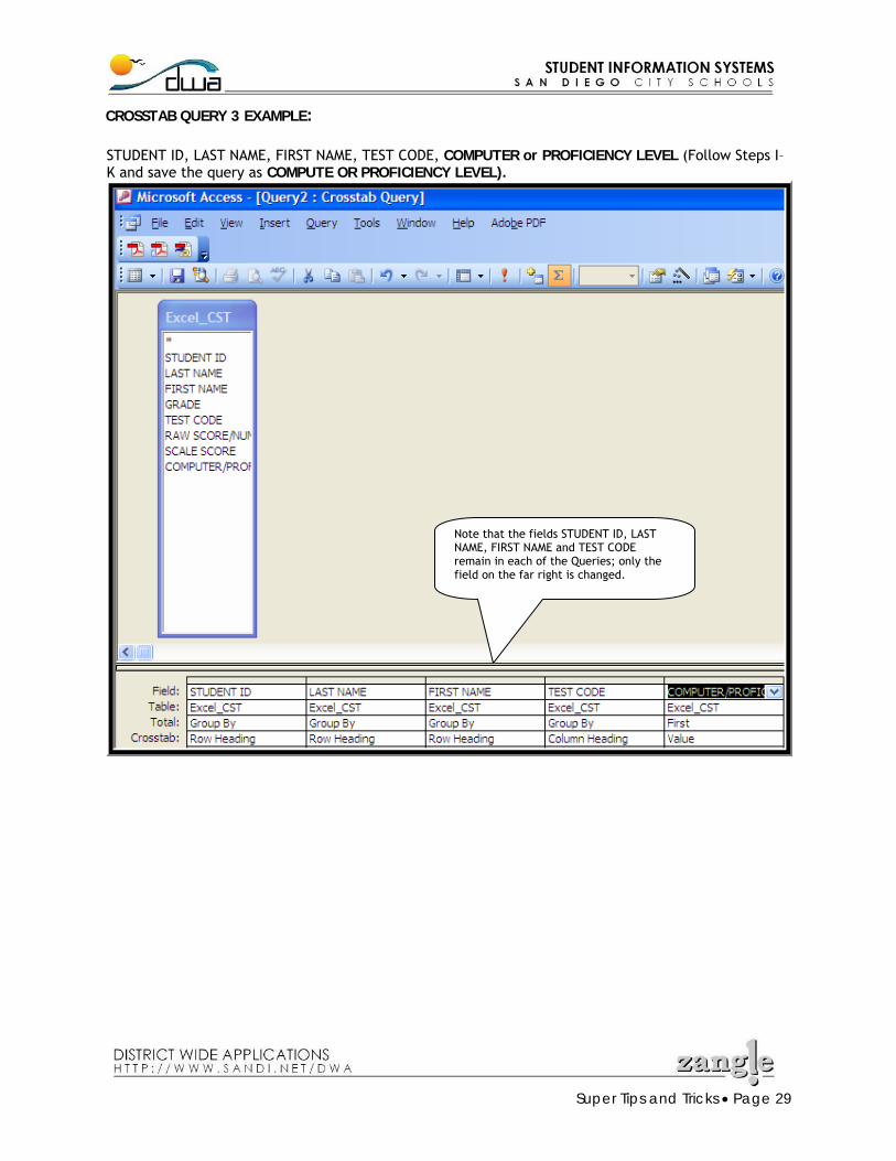
CROSSTAB QUERY 3 EXAMPLE: STUDENT ID, LAST NAME, FIRST NAME, TEST CODE, COMPUTER or PROFICIENCY LEVEL (Follow Steps I–K and save the query as COMPUTE OR PROFICIENCY LEVEL).
Note that the fields STUDENT ID, LAST NAME, FIRST NAME and TEST CODE remain in each of the Queries; only the field on the far right is changed.
Super Tips and Tricks • Page 30
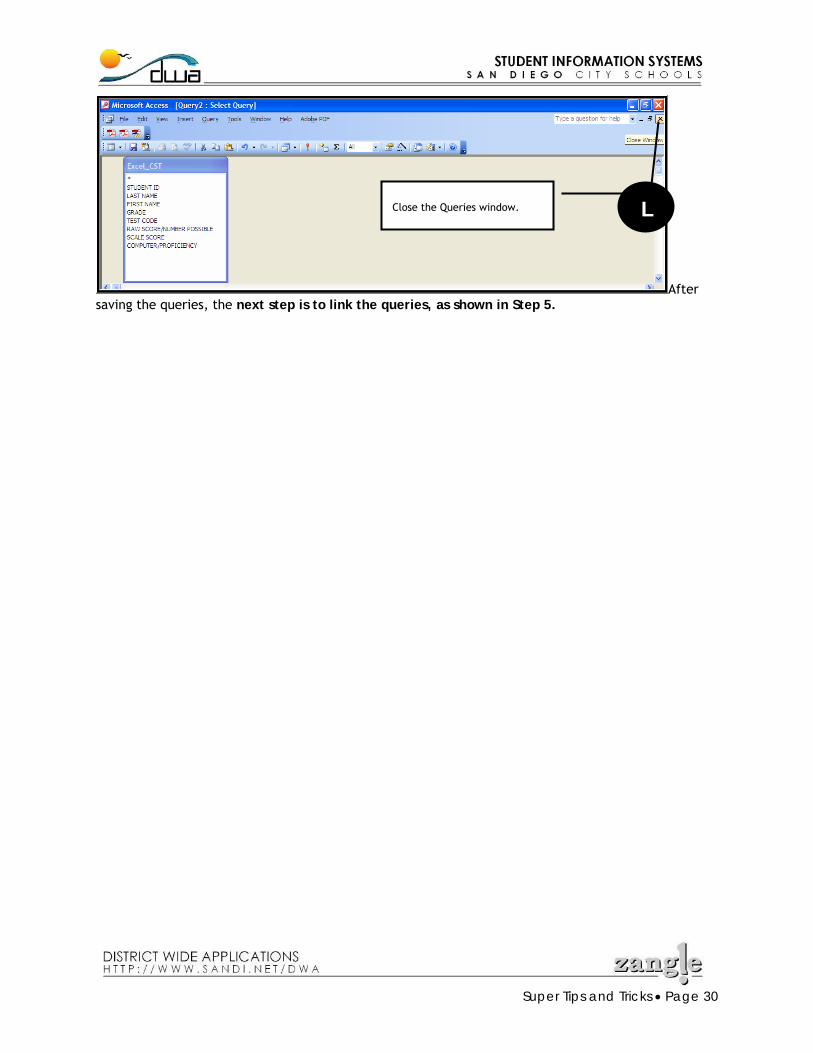
After saving the queries, the next step is to link the queries, as shown in Step 5.
L Close the Queries window.
Super Tips and Tricks • Page 31
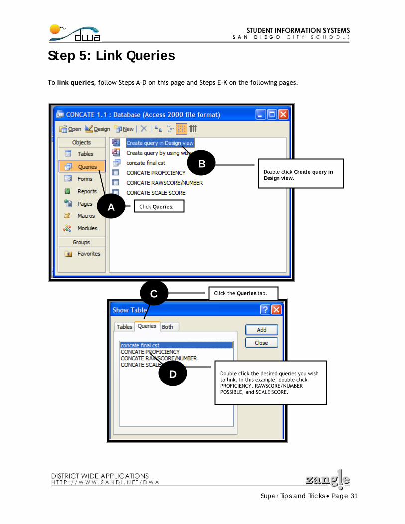
Step 5: Link Queries
To link queries, follow Steps A–D on this page and Steps E–K on the following pages.
C
Click Queries.
Double click the desired queries you wish to link. In this example, double click PROFICIENCY, RAWSCORE/NUMBER POSSIBLE, and SCALE SCORE.
Double click Create query in Design view.
A
B
Click the Queries tab.
D
C
Super Tips and Tricks • Page 32
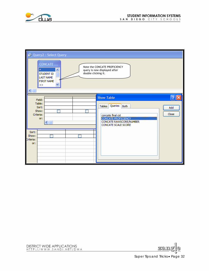
Note the CONCATE PROFICIENCY query is now displayed after double clicking it.
Super Tips and Tricks • Page 33
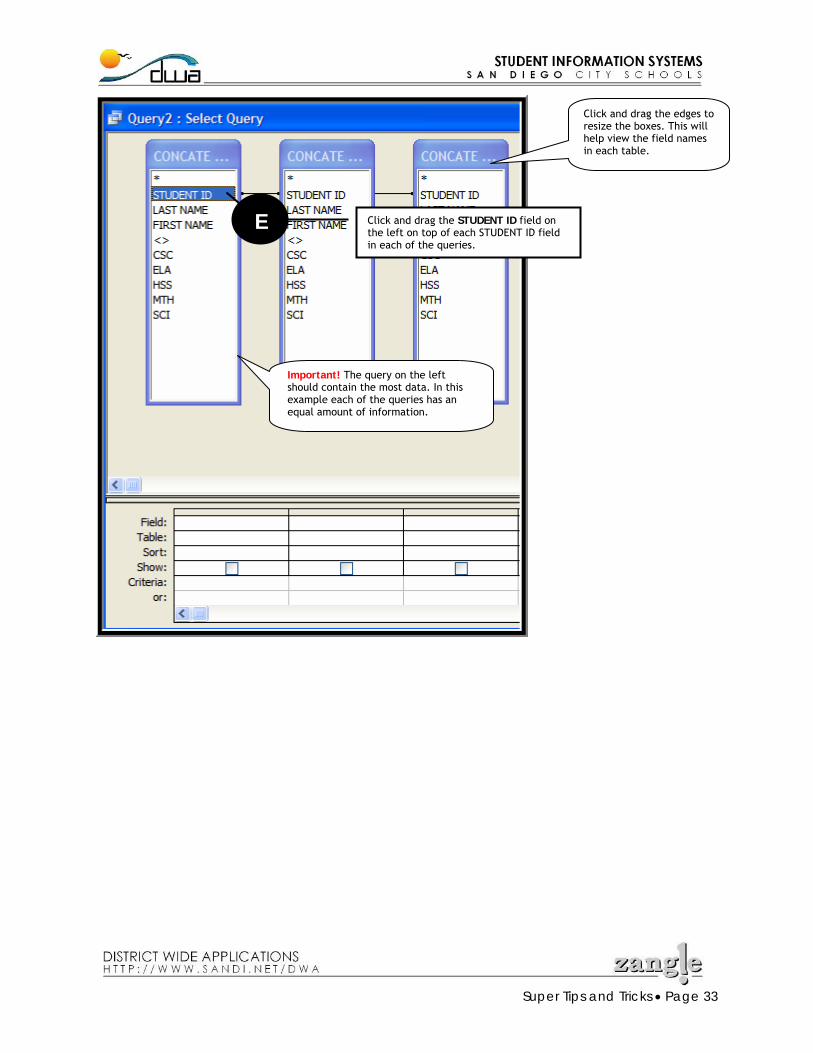
Click and drag the STUDENT ID field on the left on top of each STUDENT ID field in each of the queries.
Click and drag the edges to resize the boxes. This will help view the field names in each table.
E
Important! The query on the left should contain the most data. In this example each of the queries has an equal amount of information.
Super Tips and Tricks • Page 34
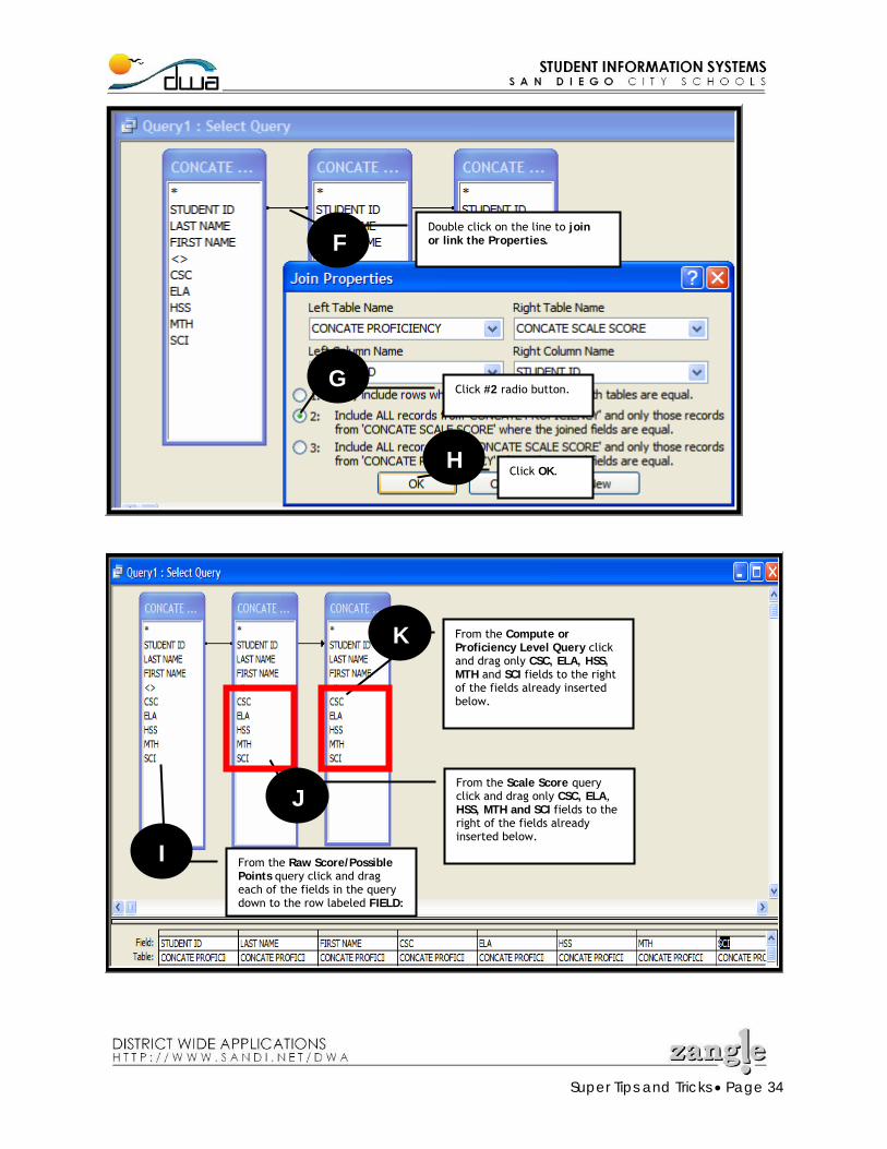
F Double click on the line to join or link the Properties.
Click #2 radio button.
G
Click OK.
H
From the Raw Score/Possible Points query click and drag each of the fields in the query down to the row labeled FIELD:
I
From the Scale Score query click and drag only CSC, ELA, HSS, MTH and SCI fields to the right of the fields already inserted below.
From the Compute or Proficiency Level Query click and drag only CSC, ELA, HSS, MTH and SCI fields to the right of the fields already inserted below.
J
K
Super Tips and Tricks • Page 35
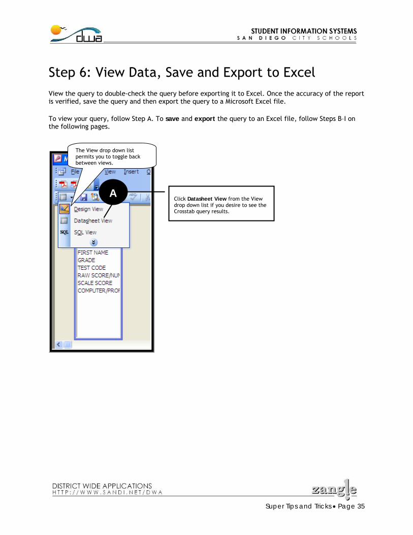
Step 6: View Data, Save and Export to Excel View the query to double-check the query before exporting it to Excel. Once the accuracy of the report is verified, save the query and then export the query to a Microsoft Excel file. To view your query, follow Step A. To save and export the query to an Excel file, follow Steps B–I on the following pages.
The View drop down list permits you to toggle back between views.
Click Datasheet View from the View drop down list if you desire to see the Crosstab query results.
A
Super Tips and Tricks • Page 36
Choose Save As from the File menu.
B
Type the desired file name. C
Click OK.
D
Super Tips and Tricks • Page 37
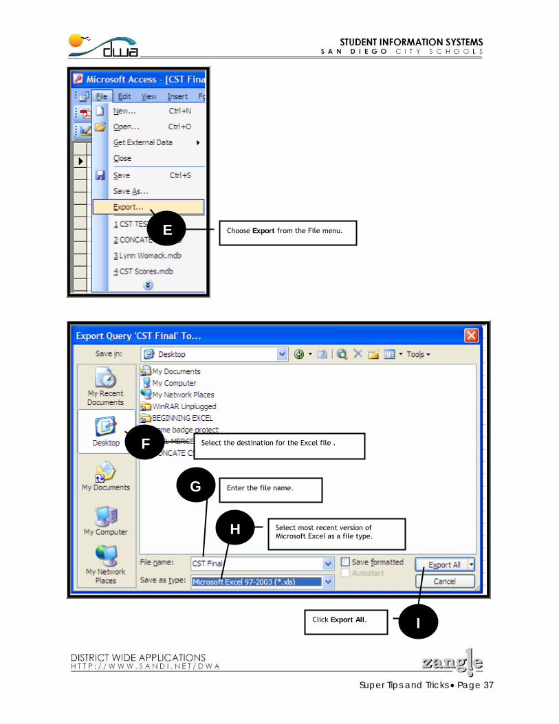
Choose Export from the File menu. E
Click Export All.
Select most recent version of Microsoft Excel as a file type.
Enter the file name.
Select the destination for the Excel file .
I
H
G
F
Super Tips and Tricks • Page 38
Clean Up Exported Excel File
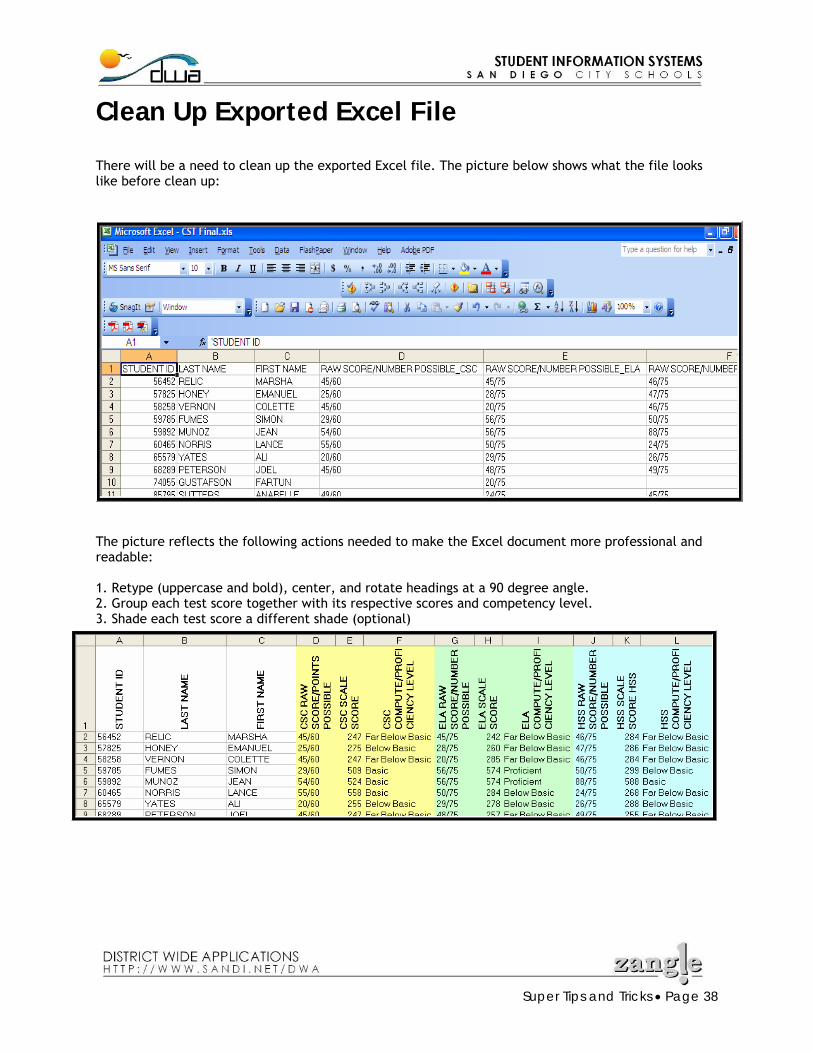
There will be a need to clean up the exported Excel file. The picture below shows what the file looks like before clean up:
The picture reflects the following actions needed to make the Excel document more professional and readable: 1. Retype (uppercase and bold), center, and rotate headings at a 90 degree angle. 2. Group each test score together with its respective scores and competency level. 3. Shade each test score a different shade (optional)
Super Tips and Tricks • Page 39
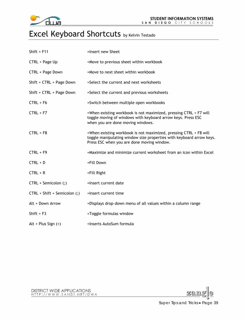
Excel Keyboard Shortcuts by Kelvin Testado
Shift + F11 =Insert new Sheet CTRL + Page Up =Move to previous sheet within workbook CTRL + Page Down =Move to next sheet within workbook Shift + CTRL + Page Down =Select the current and next worksheets Shift + CTRL + Page Down =Select the current and previous worksheets CTRL + F6 =Switch between multiple open workbooks CTRL + F7 =When existing workbook is not maximized, pressing CTRL + F7 will toggle moving of windows with keyboard arrow keys. Press ESC when you are done moving windows. CTRL + F8 =When existing workbook is not maximized, pressing CTRL + F8 will
toggle manipulating window size properties with keyboard arrow keys. Press ESC when you are done moving window.
CTRL + F9 =Maximize and minimize current worksheet from an icon within Excel CTRL + D =Fill Down CTRL + R =Fill Right CTRL + Semicolon (;) =Insert current date CTRL + Shift + Semicolon (;) =Insert current time Alt + Down Arrow =Displays drop–down menu of all values within a column range Shift + F3 =Toggle formulas window Alt + Plus Sign (+) =Inserts AutoSum formula