super-resolution video analysis for forensic investigations

Chapter 20

SUPER-RESOLUTION VIDEO ANALYSIS FOR FORENSIC INVESTIGATIONS

Ashish Gehani and John Reif

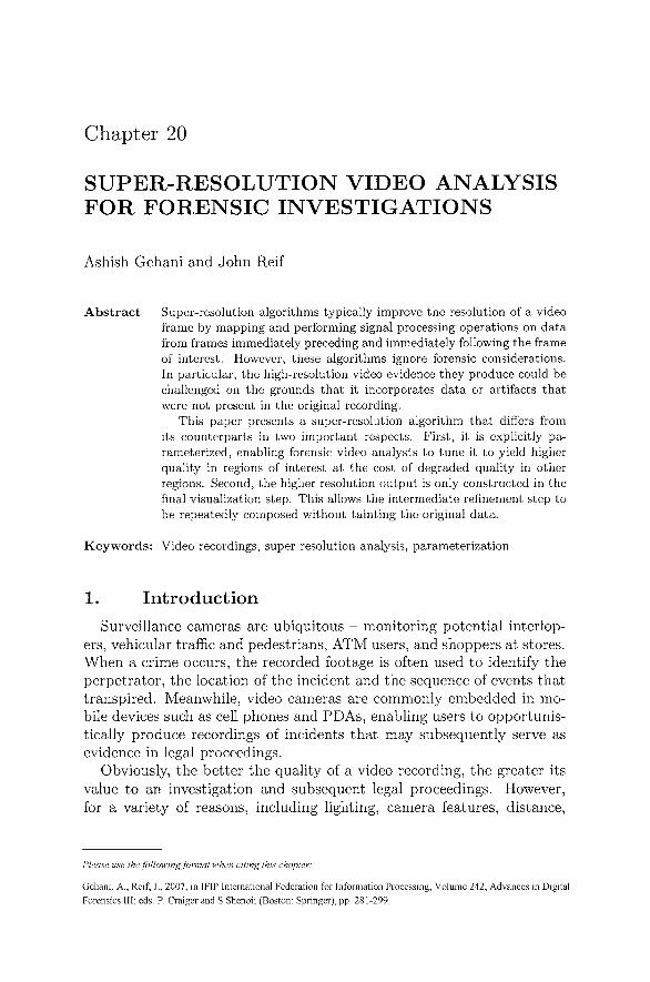
Abstract Super-resolution algorithms typically improve the resolution of a video frame by mapping and performing signal processing operations on data from frames immediately preceding and immediately following the frame of interest. However, these algorithms ignore forensic considerations. In particular, the high-resolution video evidence they produce could be challenged on the grounds that it incorporates data or artifacts that were not present in the original recording.

This paper presents a super-resolution algorithm that differs from its counterparts in two important respects. First, it is explicitly pa-rameterized, enabling forensic video analysts to tune it to yield higher quality in regions of interest at the cost of degraded quality in other regions. Second, the higher resolution output is only constructed in the final visualization step. This allows the intermediate refinement step to be repeatedly composed without tainting the original data.

Keywôrds: Video recordings, super-resolution analysis, parameterization

1. Introduction Surveillance cameras are ubiquitous - monitoring potential interlop-

ers, vehicular traffic and pedestrians, ATM users, and shoppers at stores. When a crime occurs, the recorded footage is often used to identify the perpetrator, the location of the incident and the sequence of events that transpired. Meanwhile, video cameras are commonly embedded in mo-bile devices such as cell phones and PDAs, enabling users to opportunis-tically produce recordings of incidents that may subsequently serve as evidence in legal proceedings.

Obviously, the better the quality of a video recording, the greater its value to an investigation and subsequent legal proceedings. However, for a variety of reasons, including lighting, camera features, distance,

Please use the following format when citing this chapter:

Gehani, A., Reif, J., 2007, in IFIP International Federation for Information Processing, Volume 242, Advances in Digital Forensics III; eds. P. Craiger and S Shenoi; (Boston: Springer), pp. 281-299.

282 ADVANCES IN DIGITAL FORENSICS III

angle and recording speed, a video recording may be of lesser quality, requiring it to be enhanced to provide adequate detail (resolution).

This paper describes a super-resolution algorithm that extracts data from video frames immediately preceding and following a given frame (temporal context) to improve its resolution. Super-resolution algo-rithms typically map the contextual data to a higher resolution repre-sentation, and then perform signal processing operations to improve the frame's quality. As a result, the high resolution version can be challenged on the grounds that it introduces elements not present in the original data. The algorithm presented in this paper is novel in that it maintains the additional data in an intermediate representation where every point is from an input frame; this effectively eliminates legal challenges based on the introduction of data to the original video evidence.

2. Background A digital video recording "projects" points from three-dimensional

continuous surfaces (objects in a scene) to two-dimensional finite regions (pixel elements on a sensor grid). In the process, a point in R*̂ (triple of real values that uniquely identify a location in the scene) is first mapped to a point in R^ (pair of real values that identify the registration location on the sensor grid); the set of these points constitutes the "image space." All the points that fall on a pixel in the sensor then map to a single point in N^ (pair of values that uniquely identifies the pixel's location on the sensor). The set of locations form the "representation grid." Since a collection of points in R^ combine to yield a single discrete value (pixel intensity), the set of sensor output values is called the "approximated image space."

A video sequence is formed by repeating the spatial registration pro-cess at discrete points in time. The instant in time when a frame was captured is represented with a temporal index. The temporal index is usually an integer counter. However, in the case of motion-activated recordings, the temporal index is an arbitrary strictly monotonically in-creasing sequence.

The set of points that undergoes spatial projection varies from frame to frame (Figure 1). Since points close to each other on an object are likely to have the same visual character, the human eye is unable to discern that different points are being registered. Video compression algorithms exploit this feature by replacing sets of points with single representatives. For example, quantization algorithms map a range of intensity levels to a single intensity level because it can be represented more succinctly. On the other hand, super-resolution algorithms extract

Gehani & Reif 283

Figure 1. Object sampling

Figure 2. Object mapping.

and utilize variations in tlie intensity levels to increase the detail in each video frame.

Frame resolution can be increased using spatial domain signal process-ing, e.g., linear or spline interpolation. However, these algorithms cannot recover subpixel features lost during the subsamphng process. Consec-utive frames, / j , . . . , ft+n, of a video sequence register different sets of points, 5*4,..., St+n, on the object, as illustrated in Figure 2. Therefore, super-resolution algorithms can outperform spatial domain techniques by enhancing each frame using data from temporally proximal frames.


Super-resolution algorithms have been studied for almost a decade. These algorithms use elements from a single image or video frame to construct a higher resolution version via sphne interpolation [16]. How-ever, this technique cannot recover lost subpixel features. Consequently, newer algorithms use data from several temporally proximal video frames or multiple images of the same scene. While the details differ, these algorithms employ similar observation models to characterize the degra-dation of high resolution frames to lower quality frames. As a result, the super-resolution algorithms have a similar structure [10]. The first step is coarse motion estimation, which typically estimates the motion between frames at block granularity. Next, data from contextual frames is interpolated onto a grid representing the desired high resolution out-put. The final step involves image restoration operations such as blur and noise removal.

If the motion between frames is known a priori^ low resolution frames can be spatially shifted and the resulting collection can be combined using nonuniform interpolation [17]. This can also be done when the camera aperture varies [8]. Other spatial domain algorithms use color [13] and wavelets [9]. Frequency domain approaches exploit aliasing in low resolution frames [15]. Moreover, the blur and noise removal steps may be incorporated directly [7]. Knowledge of the optics and sensor can be included to address the problem of not having sufficient low resolution frames [5]. The issue has also been addressed using maximum a posteriori (MAP) estimates of unknown values [11]. Other general approaches use projection onto convex sets (POCS) [14], iterative back-projection (IBP) [6], and adaptive filtering theory [4].

3. Motivation Super-resolution algorithms have been designed without regard to the

Frye and Daubert standards for introducing scientific evidence in U.S. courts. The Frye standard derives from a 1923 case where systolic blood pressure was used to ascertain deception by an individual. The method was disallowed because it was not widely accepted by scientists. The Frye standard was superseded in 1975 by the Federal Rules of Evidence, which require the evidence to be based in "scientific knowledge" and to "assist the trier of fact." In 1993, the Daubert family sued Mer-rell Dow Pharmaceuticals claiming that its anti-nausea drug Bendectin caused birth defects. The case reached the U.S. Supreme Court where the Daubert standard for relevancy and rehability of scientific evidence was articulated.

Gehani & Reif 285

Figure 3. Super-resolution algorithm.

Super-resolution algorithms typically map tlie contextual data to a higher resolution representation, and then perform signal processing op-erations to improve the frame's quality. As a result, the high resolution version frame can be challenged on the grounds that it introduces ele-ments not present in the original data. This is a side-effect of algorithm design, which is to use an observation model that results in an ill-posed inverse problem with many possible solutions. The algorithm introduced in this paper uses a different analytical technique that maintains the ad-ditional data in an intermediate representation where every point is from an input frame. This technique eliminates legal challenges based on the introduction of data to the original video evidence.

4. Algorithm Overview The proposed super-resolution algorithm is illustrated in Figure 3.

Each frame of a video sequence is enhanced independently in serial order. To process a given frame, a set of frames is formed by choosing several frames that are immediately previous to and immediately after the frame under consideration.

The frame being improved is then broken up into rectangular blocks. Extra data about each block in the frame is then extracted. For a given block, this is done by performing a search for one block from each of the frames in the set of frames (defined above) that best matches the


frame. A sub-pixel displacement that minimizes the error between each of the contextual blocks and the block under consideration is analytically calculated for each of the blocks in the frame.

The data thus obtained is a set of points of the form (x, y^ z)^ where z is the image intensity at point (x, y) in the XY plane. The set thus obtained corresponds to points scattered in the XY plane. To map this back to a grid, a bivariate spline surface, comprising tensor product basis splines that approximate this data, is computed. Since this is done for each frame in the sequence, a sequence similar in length to the input is produced as output.

5. Temporal Context Extraction Our algorithm enhances the resolution of a video sequence by increas-

ing the size of the data set associated with each frame. Considering the "reference frame," whose resolution is being improved, we examine the problem of extracting relevant information from only one other frame, the "contextual frame." The same process may be applied to other frames immediately before and after the reference frame in the video sequence to obtain the larger data set representing the region in object space that was mapped to the reference frame.

Ideally, whenever an object in the reference frame appears in the contextual frame, it is necessary to identify the exact set of pixels that correspond to the object, extract the set, and incorporate it into the representation of the object in the reference frame. We use a technique from video compression called "motion estimation" for this purpose.

5,1 Initial Motion Estimation The reference frame is broken into blocks of fixed size (the block di-

mensions are an algorithm parameter). The size of the block must be determined as a function of several factors that necessitate a tradeoff. Smaller blocks provide finer granularity, allowing for local movements to be better represented. The uniform motion field is forced on a smaller number of pixels, but this increases the computational requirements. Depending on the matching criterion, smaller blocks result in more in-correct matches. This is because larger blocks provide more context, which increases the probability of correctly determining an object's mo-tion vector.

For each block, a search for a block of identical dimensions is per-formed in the contextual frame. A metric that associates costs inversely with the closeness of matches is used to identify the block with the lowest cost. The vector, which connects a point on the reference block to the

Geham & Reif 287

corresponding point of the best match block in the contextual frame, is denoted as the initial motion estimate for the block.

Matching Criteria If a given video frame has width Fyj and height F/^, and the sequence is T frames long, then a pixel at position {m,n) in the /^^ frame, is specified by VS{m,n, f), where m G { 1 , . . . ^Fy^}, n G {!,... ,i^/i}, and / G { 1 , . . . ,T}. If a given block has width J5-̂ ; and height S/^, then a block in the reference frame with its top left pixel at (x, y) is denoted RB{x^ y, t), where x G { 1 , . . . , {Fy^ — B^, + 1)}, y G {!,..., {Fh — Bh •\- 1)}, and t is the temporal index. For a fixed reference frame block denoted by RB{x^y->'^)i the block in the contextual frame that has its top left pixel located at the position (x + a, y + 6) is denoted by CB{a,h,u), where (x + a) G {!,... ^{F^j — B^; + 1)}, {y -\- h) G {!,..., (F^ — B/i + 1)}, and where the contextual frame has temporal index [t -\- u). The determination that the object, represented in the block with its top left corner at (x, y) at time t, has been translated in exactly u frames by the vector (a, 6), is associated with a cost given by the function C{RB{x, y, t), CB{a, 6, u)).

We use the mean absolute difference (MAD) as the cost function. Empirical studies related to MPEG standards show that it works just as eff'ectively as more computationally intensive criteria [1]. The corre-sponding cost function is given by:

MAD{RB{x,y,t),CB{a,b,u)) = (1) ^ ( B . a ; - l ) ( B h - l )

BwBh 1=0 j~Q

Motion Vector Identification Given a reference block RB{x^y^t), we wish to determine the block CB[a^ 6, u) that is the best match in the (t-\-uy^ frame, with the motion vector (a, b) constrained to a fixed rect-angular search space centered at (x,i/). This is illustrated in Figure 4. If the dimensions of this space are specified as algorithm parameters p and g, then a G {(x—p) , . . . , (x-f-p)}, and b G {{y — q),..., {y^-q)} must hold. These values can be made small for sequences with little motion to enhance computational efficiency. If the motion characteristics of the sequence are unknown, p and q may be set so that the entire frame is searched.

The "full search method" is the only method that can determine the best choice CB{amin^^min->u) without error, such that:


Figure 4- Contextual block determined with integral pixel accuracy.

Voe {(-x + l ) , , . . , { F „ - B „ - . T + l ) } , (2)

-ib e {{-y + 1),... ,{FH -^ Bh - y + 1)}, C{RB{x,y, t), CB{amrn, b-min,u)) < C{RB{x,y, t), CB(a, b,u))

The method computes C{RB{x, y, t),CB{a, b, u)) for all values of a and b in the above mentioned ranges and keeps track of the pair (a, b) that results in the lowest cost. The complexity of the algorithm is 0{pqBwBh) when p and q are specified, and 0{FwFfiByjBh) when the most general form is used.

5.2 Re-Estimation with Subpixel Accuracy Objects do not move in integral pixel displacements. It is, therefore,

necessary to estimate the motion vector at a finer resolution. This is the second step in our hierarchical search.

Our analytical technique for estimating the motion of a block with sub-pixel accuracy is illustrated in Figure 5. By modeling the cost func-tion as a separable function, we develop a measure for the real-valued displacements along each orthogonal axis that reduce the MAD value.

Let the function !F{x, y) contain a representation of the reference frame with temporal index t, i.e.,

V-re { l , . . . ,F„},Vy 6 { l , . . . , F h } (3) r[x,y) = VSix,y,t)

Geham & Reif 289

Figure 5. Sub-pixel displacement to improve reference area match.

Furthermore, let the function G{x, y) contain a representation of the contextual block for which the motion vector is being determined with sub-pixel accuracy. If RB{xo,yo,t) is the reference block for which the previous stage of the algorithm found CB{amin,bmimu) to be the con-textual block with the closest match in frame {t + u), then define:

Xmin = 3^0 'v (^min, Xmax ^ ^0 r Q'min + i^w J- (4j

ymin ^^ yo y Omin i ymax ^^ 't/0 + Omin i i^h t

Note that the required definition of Q{x,y) is given by:

vX t \Xmin i • . - j ^max }yye{y mm ) • • • ,ymax} (5)

Q{x,y) = VS{x,y,u)

Instead of iamin,bmin), which is the estimate that results from the first stage of the search, we seek to determine the actual motion of the object that can be represented by {amin + ôLmvm bmin + 5bmin)- Therefore, at this stage the vector {Samin, ^bmin), which we call the "sub-pixel motion displacement," must be found.

LEMMA 1 Sx can be calculated in C(log (YBwBh)) space and 0{Bu,Bh) time.

Proof: This statement holds when the intensity values between two adjacent pixels are assumed to vary linearly. Note that Y is the range


of possible values of the function (or the range of possible values of a pixel's color).

If the sub-pixel motion displacement is estimated as (5x, 5y), then the cost function is C{RB{x^ y, t), CB{a + 5x,b -]- Sy,u)). We can use mean square error (MSE) as the matching criterion and treat it as an indepen-dent function of 5x and 6y. We apply linear interpolation to calculate J^ and G with non-integral parameters. To perform the estimation, the function must be known at the closest integral-valued parameters. Since the pixels adjacent to the reference block are easily available, and since this is not true for the contextual block, we reformulate the above equa-tion without loss of generality as:

MSE{5x)= £ g {T{x + Sx,y)-g{x,y)f (6)

This is equivalent to using a fixed grid (contextual block) and variably displacing the entire reference frame to find the best sub-pixel displace-ment (instead of intuitively fixing the video frame and movement of the block whose motion is being determined).

Assuming that the optimal sub-pixel displacement along the x axis of the contextual block under consideration is the 5x that minimizes the function MSE{6x), we solve for 6x using the constraint:

^ MSE{Sx) = 0 (7) d{Sx)

Xmax y-maa

X — ̂ min y — Vmin

\T(x -\-bx,y)- g(x,y)] -^Tj^î^ + Sx,y)

Since T{x^y) is a discrete function, we use linear interpolation to ap-proximate it as a continuous function for representing J^{x + 6x^y) and computing -MJ^^{X -f Sx^ y). We now consider the case of a positive 5x.

\/5x, 0 < (5x < 1, T{x + 5x, y) - J^(a;, y) + 5x [r{x + 1, y) - ^{x, y)] (8)

^ J'{x-^5x,y):=r{x^l,y)-jF{x,y) (9) d{5x)

By rearranging terms, we obtain the closed form solution:

6x ^ (10) E ^ - ; , , T^lTyl,^ [ [H^ + 1 . y) - Hx. y)] [^(^, y) - g(^, y)] ]

Gehani & Reif 291

Similarly, an independent calculation can be performed to ascertain the negative value of 6x that is optimal. The solution for the case of a negative 5x is a minor variation of the technique described above. Finally, the MSE between the reference and contextual block is com-puted for each of the two 6x's. The Sx that results in the lower MSE is determined to be the correct one.

The closed form solution for each dx adds ByjB^ terms to the nu-merator and the denominator. Each term requires two subtractions and one multiplication. This is followed by computing the final quotient of the numerator and denominator summations. Therefore, the time com-plexity is 0{B^Bh). Note that computing the MSE is possible within this bound as well. Since the function values range up to Y and only the running sum of the numerator and denominator must be stored, the space needed is OilogYByjBk)- •

We now show that it is possible to obtain a better representation of a block in the reference frame by completing the analysis of sub-pixel displacements along the orthogonal axis.

LEMMA 2 The cardinality of the set of points that represents the block under consideration from the reference frame is non-decreasing.

Proof: After a 5x has been determined, the block must be translated by a quantity 5y along the orthogonal axis. It is important to perform this calculation after the 5x translation has been applied because this guarantees that the MSE after both translations is no more than the MSE after the first translation; this ensures algorithm correctness. The 5y can be determined in a manner analogous to fe, using the represen-tation of the MSE below with the definition x' — x -]- 5x. The closed form for a positive 5y is defined below. The case when 5y is negative is a minor variation.

\/5y, 0<6y<l,5y= (11)

E^^SLn ^y^g ln [ [nx'.y + 1) - Hx'.y)] [H^'^y) - Q{x',y)] ]

Z:zz.Êlzz^^ IH^'^y +1) -H '̂̂ y)]'

If the sub-pixel displacement {5x,5y) results in an MSE between the contextual and reference blocks exceeding a given threshold, then the extra information is not incorporated into the current set representing the reference block. This prevents the contamination of the set with spurious information. It also completes the proof that either a set of points that enhances the current set is added, or none are - since this


yields a non-decreasing cardinality for the set representing the block being processed. D

By performing this analysis independently for each of the contextual blocks that corresponds to a reference block, we obtain a scattered data set representing the frame whose resolution is being enhanced. If the sampling grid were to have infinite resolution, an inspection of the values registered on it at the points determined to be in the image space would find the data points to be a good approximation. By repeating this process with a number of contextual frames for each reference frame, we can extract a large set of extra data points in the image space of the reference frame. At this stage, the resolution of the video frame has been analytically enhanced. However, the format of scattered data is not acceptable for most display media (e.g., video monitors). Therefore, the data must be processed further to make it usable.

6. Coherent Frame Creation We define a "uniform grid" to be the set Hp^k U VQ.I of liiies in R^,

where Hp^^ = {x = /ca | /c G {0,1, 2 , . . . , P } , a G R, F G N } specifies a set of vertical lines and VQÎ = {T/ = //? | / G {0,1, 2 , . . . , Q}, /? G R, Q G N } specifies a set of horizontal lines. Specifying the values of P^Qâ^ and P determines the uniform grid uniquely. Given a set S of points of the form {x,y,z), where z represents the intensity of point (x,y) in image space, if there exist M, N, a, and (3 such that all the (x, y) of the points in the set S lie on the associated uniform grid, and if every data point (x, y) on the uniform grid has an intensity (that is a 2: component) associated with it, then we call the set S a "coherent frame." Each of the frames in the original video sequence was a coherent frame. We seek to create a coherent frame from the data set D^ with the constraint that the coherent frame should have the same number of points as the data set D,

The general principle used to effect the transformation from scattered data to a coherent frame is to construct a surface in R^ that passes through the input data. By representing this surface in a functional form with the X and y coordinates as parameters, it can then be evaluated at uniformly-spaced points in the XY plane to produce a coherent frame.

Numerous methods are available for this purpose, the tradeoff be-ing the increased computational complexity needed to guarantee greater mapping accuracy. While the efficiency of the procedure is important, we would like to make our approximation as close a fit as possible. Note that although we will be forced to use interpolation techniques at this stage, we are doing so with a data set that has been increased in size.

Gehani & Reif 293

so this is not equivalent to performing interpolation at the outset and is certainly an improvement over it. We use B-spline interpolation with degree /c, which can be set as a parameter to our algorithm.

7. Implementation Issues Given an arbitrary scattered data set, we can construct a coherent

frame that provides a very good approximation of the surface specified by the original data set. However, if we were to work with the entire data set at hand, our algorithm would not be scalable due to the memory requirements.

Noting that splines use only a fixed number of neighboring points, we employ the technique of decomposing the data set into spatially related sets of fixed size. Each set contains all the points within a block in image space. The disadvantage of working with such subsets is that visible artifacts develop at the boundaries in the image space of these blocks.

To avoid this we "compose" the blocks using data from adjacent blocks to create a border of data points around the block in question, so that the spline surface constructed for a block is continuous with the surfaces of the adjacent blocks. Working with one block at a time in this manner, we construct surfaces for each region in the image space, and evaluate the surface on a uniform grid, to obtain the desired representation. A coherent frame is obtained when this is done for the entire set.

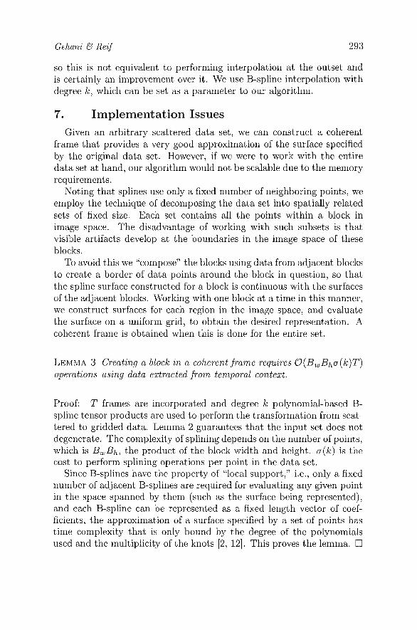
LEMMA 3 Creating a block in a coherent frame requires 0{B^Bha{k)T) operations using data extracted from temporal context.

Proof: T frames are incorporated and degree k polynomial-based B-spline tensor products are used to perform the transformation from scat-tered to gridded data. Lemma 2 guarantees that the input set does not degenerate. The complexity of splining depends on the number of points, which is BujBh, the product of the block width and height. a{k) is the cost to perform sphning operations per point in the data set.

Since B-splines have the property of "local support," i.e., only a fixed number of adjacent B-splines are required for evaluating any given point in the space spanned by them (such as the surface being represented), and each B-sphne can be represented as a fixed length vector of coef-ficients, the approximation of a surface specified by a set of points has time complexity that is only bound by the degree of the polynomials used and the multiphcity of the knots [2, 12]. This proves the lemma. D


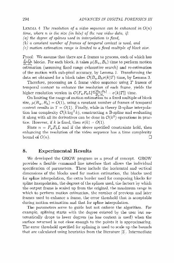
LEMMA 4 The resolution of a video sequence can he enhanced in 0{n) time, where n is the size (in bits) of the raw video data, if: (a) the degree of splines used in interpolation is fixed, (h) a constant number of frames of temporal context is used, and (c) motion estimation range is limited to a fixed multiple of block size.

Proof: We assume that there are L frames to process, each of which has ^^^ blocks. For each block, it takes ii{Bw, B^) time to perform motion estimation (assuming fixed range exhaustive search) and re-estimation of the motion with sub-pixel accuracy, by Lemma L Transforming the data set obtained for a block takes 0{ByjBhcr{k)T) time, by Lemma 3.

Therefore, processing an L frame video sequence using T frames of temporal context to enhance the resolution of each frame, yields the higher resolution version in 0 ( F ^ F ^ L [ ^ ^ | j / ^ ^ + cr(/c)T]) time.

On limiting the range of motion estimation to a fixed multiple of block size, /i(B^^Bh) = 0(1) , using a constant number of frames of temporal context results in T == 0(1) . Finally, while in theory B-spline interpola-tion has complexity 0{klog^ k), constructing a B-spline and evaluating it along with all its derivatives can be done in 0{k'^) operations in prac-tice. However, if k is fixed, then a{k) = 0(1) .

Since n = F^jF^L and if the above specified constraints hold, then enhancing the resolution of the video sequence has a time complexity bound of 0 ( n ) . D

8. Experimental Results We developed the GROW program as a proof of concept. GROW

provides a flexible command fine interface that allows the individual specification of parameters. These include the horizontal and vertical dimensions of the blocks used for motion estimation, the blocks used for spline interpolation, the extra border used for composing blocks for spline interpolation, the degrees of the splines used, the factors by which the output frame is scaled up from the original, the maximum range in which to perform motion estimation, the number of previous and later frames used to enhance a frame, the error threshold that is acceptable during motion estimation and that for spline interpolation.

The parameters serve to guide but not enforce the algorithm. For example, splining starts with the degree entered by the user but au-tomatically drops to lower degrees (as less context is used) when the surface returned is not close enough to the points it is approximating. The error threshold specified for splining is used to scale up the bounds that are calculated using heuristics from the literature [3]. Intermediate

Gehani & Reif 295

results, such as sub-pixel displacements, are calculated and kept in high precision floating point format. When error thresholds are crossed, the data in question is not used. Thus, occlusion and peripheral loss of ob-jects are dealt with effectively using only reference image data for the relevant region.

To evaluate the performance of GROW, we use the signal-to-noise ratio (SNR) to measure distortion:

In the definition, G represents the high resolution video sequence, and J^ represents the high resolution sequence obtained by running GROW on the low resolution version associated with G- The low resolution version is obtained through the sub-sampling of Q.

Table 1. Effect of parameter variations on output frame SNR.

Super-Resolution Technique s t p 1 SNR

Spline Interpolation (w/o Temporal Context) 16 16 0 0 28.39 Spline Interpolation (w Temporal Context) 8 8 2 2 30.40 Spline Interpolation (w Temporal Context) 4 4 2 2 30.59

Table 1 compares the signal strengths of the sequence produced by GROW for various parameters: the range for initial motion estimation on each axis (5, t) and the number of previous and later frames used (p, I). The first row represents the use of spline interpolation with 16x16 motion estimation blocks (s, t = 16) and no proximal frames (p, / = 0). The second row, corresponding to the use of 8x8 motion estimation blocks and two previous (p = 2) and two later (/ = 2) frames (five frames total), results in a noticeably higher SNR. The third row, with 4x4 mo-tion estimation blocks and five total frames, shows further improvement in the SNR, but at the cost of increased computation.

Figure 6 shows five frames of a video sequence. The higher resolution output corresponding to the third frame in Figure 6 is generated using all five frames as input to GROW.

Figure 7(a) shows the original frame whose resolution is being in-creased. Figure 7(b) shows the result of spline interpolation. Figure 7(c) shows the frame obtained by applying GROW. Artifacts that arise in the final images are due to errors in initial block matching and sphning. Forensic video analysts can tolerate these artifacts in portions of the


Figure 6. Original frames.

Figure 7. (a) Original frame; (b) Higher resolution version using spline interpolation; (c) Higher resolution version using GROW.

frame that are of no consequence; in exchange they get greater detail in regions of interest.

Certain aspects, such as sphne degree selection, have been automated in GROW. Others, such as splining error bounds, are semi-automatically calculated using heuristics and minimal user input. To obtain an optimal image sequence, it is necessary for the user to manually adjust the val-ues fed into the algorithm. Significantly better results can be obtained by hand tuning GROW than by applying spline interpolation without temporal context. This is clear from the results in Table 1, where spline

Gehani & Reif 297

Figure 8. Time requirements (Splining (SGF); Temporal context extraction (TCE).

interpolation without proximal frames (first row) does not yield as strong a signal as the best case output of GROW (third row).

Note that the improvement in spline interpolation by adding temporal context is accomplished at little cost. This is verified in the graphs in Figure 8, where the time requirement for temporal context extraction is minimal compared with that for spline construction and evaluation.

9. Conclusions This paper describes how temporally proximal frames of a video se-

quence can be utilized to aid forensic video analysts by enhancing the resolution of individual frames. The super-resolution technique enables video analysts to vary several parameters to achieve a tradeoff between the quality of the reconstructed regions and the computational time. Another benefit is that analysts can further enhance regions of interest at the cost of degrading other areas of a video frame. Moreover, tempo-ral extraction is performed first, with the mapping to a regular grid only occurring for visualization at the end. This is important for maintaining the integrity of evidence as video frames may be processed repeatedly without tainting the intermediate data.

References

[1] V. Bhaskaran and K. Konstantinides, Image and Video Com-pression Standards: Algorithms and Architectures^ Kluwer, Boston, Massachusetts, 1996.

[2] C. de Boor, A Practical Guide to Splines, Springer-Verlag, New York, 1978.


[3] P. Dierckx, Curve and Surface Fitting with Splines, Oxford Univer-sity Press, New York, 1993.

[4] M. Elad and A. Feuer, Super-resolution restoration of an image sequence: Adaptive filtering approach, IEEE Transactions on Image Processing, vol. 8(3), pp. 387-395, 1999.

[5] R. Hardie, K. Barnard, J. Bognar, E. Armstrong and E. Watson, High-resolution image reconstruction from a sequence of rotated and translated frames and its appUcation to an infrared imaging system. Optical Engineering, vol. 37(1), pp. 247-260, 1998.

[6] M. Irani and S. Peleg, Improving resolution by image registration. Computer Vision, Graphics and Image Processing: Graphical Mod-els and Image Processing, vol. 53(3), pp. 231-239, 1991.

[7] S. Kim, N. Bose and H. Valenzuela, Recursive reconstruction of high resolution image from noisy undersampled multiframes, IEEE Transactions on Acoustics, Speech and Signal Processing, vol. 38(6), pp. 1013-1027, 1990.

[8] T. Komatsu, T. Igarashi, K. Aizawa and T. Saito, Very high res-olution imaging scheme with multiple different-aperture cameras. Signal Processing: Image Communication, vol. 5(5-6), pp. 511-526, 1993.

[9] N. Nguyen and P. Milanfar, An efficient wavelet-based algorithm for image super-resolution, Proceedings of the International Conference on Image Processing, vol. 2, pp. 351-354, 2000.

[10] S. Park, M. Park and M. Kang, Super-resolution image reconstruc-tion: A technical overview, IEEE Signal Processing, vol. 20(3), pp. 21-36, 2003.

[11] R. Schulz and R. Stevenson, Extraction of high-resolution frames from video sequences, IEEE Transactions on Image Processing, vol. 5(6), pp. 996-1011, 1996.

[12] L. Schumaker, Spline Functions: Basic Theory, Wiley, New York, 1981.

[13] N. Shah and A. Zakhor, Resolution enhancement of color video sequences, IEEE Transactions on Image Processing, vol. 8(6), pp. 879-885, 1999.

[14] H. Stark and P. Oskoui, High resolution image recovery from image-plane arrays using convex projections. Journal of the Optical Society of America, vol. 6(11), pp. 1715-1726, 1989.

Gehani & Reif 299

[15] R. Tsai and T. Huang, Multiple frame image restoration and reg-istration, in Advances in Computer Vision and Image Processing, T. Huang (Ed.), JAI Press, Greenwich, Connecticut, pp. 317-399, 1984.

[16] M. Unser, A. Aldroubi and M. Eden, Enlargement or reduction of digital images with minimum loss of information, IEEE Transac-tions on Image Processing, vol. 4(3), pp. 247-258, 1995.

[17] H. Ur and D. Gross, Improved resolution from sub-pixel shifted pic-tures. Computer Vision, Graphics and Image Processing: Graphical Models and Image Processing, vol. 54(2), pp. 181-186, 1992.

Documents

super-resolution video analysis for forensic investigations