1

Super linear speedup in a local parallel

meshless solution of thermo-fluid problems

G. Kosec, M. Depolli, A. Rashkovska, R. Trobec

Jožef Stefan Institute, Department of Communication Systems, Jamova 39 1000 Ljubljana, Slovenia

gkosec@ijs.si, matjaz.depolli@ijs.si, aleksandra.rashovska@ijs.si, roman.trobec@ijs.si

Abstract

The performance of the parallel implementation of the local meshless numerical method in

solving system of coupled partial differential equations is explored. Presented numerical

approach makes the computation convenient for parallel implementation using OpenMP based

parallelization. The numerical experiments are performed on the de Vahl Davis natural

convection case, with superlinear computational speedup regime identified. The phenomenon is

further investigated through measurements of the central processing unit cache hit rates. It is

demonstrated that the accumulation of L3 caches governs the superlinear speedup. Considering

the presented analyses basic rules for effective computation strategy regarding the multicore

computations are suggested.

Keywords:

multicore; cache; OpenMP; superlinear speedup; Meshless; natural convection

1. Introduction

Numerical analysis and computer modelling are becoming basic tools for technological and

scientific research. Numerous problems, e.g. fluid flow, various transport phenomena, weather

dynamic, etc. require adequate discretization techniques to be addressed. In the majority of

numerical simulations the Finite Volume Method (FVM) [1], the Finite Difference Method

(FDM) [2], the Boundary Element Method (BEM) [3] or the Finite Element Method (FEM) [4]

are used. However, in the last few years new class of numerical methods, referred to as the

meshless methods [5] is becoming popular as an alternative. The treatment of complex

geometries is within the meshless framework much simplified since no topological relations

between computational nodes are needed. Several different meshless methods exist [6-8] and this

work is focused on one of the simplest among them - the point interpolation [9] Local Radial

Basis Function Collocation Method (LRBFCM) [10]. The main advantage of the local numerical

method is that the system matrix remains sparse or banded, which simplifies the solution

procedure. In contrast, a global approach [11] might become instable for increasing number of

discretization points, demands a lot of computational resources, and complicates the computer

program implementation. Besides the simpler formulation, the local solution procedure also

enables higher parallel efficiency. From the computation point of view, the localization reduces

inter-processor communication, which is often a bottleneck of parallel algorithms [12]. The

computation time is an important factor in numerical simulations and it is often not addressed

2

adequately. An important part of the numerical approach is thus the effective implementation of

the solution procedure on modern computer architectures. The developments in the technology

of the computer architectures are nowadays extremely vivid. The processing power can be

increased either by increasing the processor’s clock frequency or by increasing the number of

processing units. The clock frequencies are approaching their physical limits; therefore the

second option - increased number of processing units - is becoming more attractive. Parallel

computers, available today in most desktop computers or computer servers, can compensate for

the lack of performance of a single computer, but only in cases where an efficient parallelization

of the computational method is known. Various application programming interfaces (APIs) for

parallel programming are used to maximize the performance of parallel systems. Nowadays, the

most widely used APIs for parallel programming are MPI for distributed-memory systems, and

Ptreads and OpenMP for shared-memory systems [13]. Moreover, using graphical processing

units (GPUs) for solving parallel problems is widely spreading. APIs that support parallel

programming on GPUs are becoming more and more popular, like CUDA and OpenCL [14, 15].

There are several publications regarding the parallelization of different numerical schemes for

various applied problems [12, 16-18], mostly based on MPI parallelization, but only a few

numerical studies tackle the influence of the cache memory effects on the performance of

parallel computations [19].

In this paper, we demonstrate the efficiency of an OpenMP [20] based parallel implementation of

the completely local meshless solution of the classical de Vahl Davis benchmark test case [21]

on a multicore multiprocessor architecture. The paper contributes two basic messages. First, the

parallelization of the proposed meshless based numerical scheme is straightforward on shared-

memory systems. A minor amount of effort and expertise are required to apply OpenMP

parallelization if the sequential code is ready, thus the approach is interesting for engineering

computations. On the other hand, the method offers several convenient features, like ease of

implementation, stability, accuracy, and good convergent behaviour [22] that have been already

successfully proved on several demanding non-linear coupled problems [23-25] .

Second, the efficiency of a parallel implementation can be gravely affected by the memory

architecture of a computational system. It is demonstrated that extreme superlinear speedup can

be achieved if appropriate architecture is used for a specific problem size. The effect is explained

by measurements of the central processing unit (CPU) counters through execution of a

simulation. It is clearly shown that accumulating L3 caches govern the effect. In other words, it

is not only the power of CPU that matters in intense simulations; communication speed is

equally important.

The rest of the paper is organized as follows. In section 2 the test problem is described. Next, the

meshless solution methodology and LBRFCM are briefly presented, followed by description of

the parallel program implementation. Section 5 is devoted to the analysis and interpretation of

the obtained experimental results. Concluding section summarizes the results and provides

suggestions for the users dealing with complex realistic numerical problems.

3

2. Governing equations

The most standard free fluid flow benchmark test is the well-known de Vahl Davis natural

convection test [21]. There are several numerical solutions published in the literature [24, 26, 27]

that make the tests convenient for benchmarking purposes. The problem domain is a closed air-

filled square-shaped cavity with differentially heated vertical walls with temperature difference

T and insulated horizontal walls. Non-permeable and no-slip velocity boundaries are assumed.

The problem dynamics is described by three coupled Partial Differential Equations (PDEs)

equations: mass (1), momentum (2) and energy conservation (3) equations, where all material

properties are considered to be constant. The Boussinesq approximation (4) is used for the

treatment of the body force in the momentum equation. The natural convection is thus described

by the following system of equations

0 v , (1)

( ) Pt

vvv v b , (2)

( )

p

p

c Tc T T

t

v, (3)

ref1 ( )T T T b g , (4)

with ref, , , , , , , , , ,p Tu v P T c T v g and b standing for velocity, pressure, temperature,

thermal conductivity, specific heat, gravitational acceleration, density, coefficient of thermal

expansion, reference temperature for Boussinesq approximation, viscosity and body force,

respectively. The thermo-physical properties are assumed constant in the de Vahl Davis case.

The case is characterized by two dimensionless values

3 2

Ra=T H pT c

g, (5)

Prpc

, (6)

referred as Rayleigh and Prandtl numbers, respectively. ,H W stands for the domain dimension

(Figure 1).

4

Figure 1: The geometry and boundary conditions of natural convection benchmark test.

3. Solution procedure

In this work, we focus on a local meshless numerical method with a local pressure-velocity

coupling. The general idea behind the method is the use of local sub clusters of discretization

nodes termed as local support domains (Figure 2). Within a selected support domain, an arbitrary

field is approximated as a linear combination of weighted basis functions

1

( ) ( )N

n n

n

p p , (7)

where , , and , ,n n x yN p p p stand for the approximation function, the number of basis

functions, the approximation coefficients, the basis functions and the position vector,

respectively. Such an approximation function is created in each discretization point. Considering

the analysis from Franke [28], we use Hardy’s Multiquadrics (MQs) for the basis functions. We

use the collocation approach, i.e. the number of support points is the same as the number of the

basis functions. After the solution of local systems, i.e. determination of unknown coefficients α

the arbitrary spatial differential operation L can be evaluated (7)

1

( )N

n n

n

L L

p p . (8)

The computation of the coefficients and the evaluation of the differential operators can be

combined in a single operation. The differential operator Lχ vector is introduced as

1

1

( ) ( )N

L

m nm n

n

L

p p (9)

and a differential operation is thus simplified to

1

( )N

L

m n

n

L

p p p . (10)

5

The structured formulation is convenient for implementation since most of the complex and CPU

demanding operations are performed in the pre-process phase. The Neumann boundary

conditions are computed directly by equation (10) while the Dirichlet conditions are explicitly

set. More details about the presented spatial discretization can be found in [29].

Figure 2: Schematic representation of the meshless numerical principle.

The temporal discretization is done through a two-level explicit time stepping

00 0 0 0 0 0 0D S

t

v , (11)

where the zero-indexed quantities stand for the values at the previous time step, and ,D S for the

general diffusion coefficient and the source term, respectively. The time step is denoted with t .

The pressure-velocity coupling is performed through the correction of the intermediate velocity

0 0 0 0 0 0ˆ ( )

tP

v v v b v v . (12)

Equation (12) does not take into account the mass continuity. In order to drive velocity to the

solenoid field the iteration is introduced. In each iteration, the pressure is corrected as

1ˆ ˆm mP P P , (13)

where andm P stand for the iteration index and the pressure correction, respectively. The

pressure correction is directly related to the divergence of the intermediate velocity

ˆ mP

t

v , (14)

where stands for the relaxation coefficient. The corrected pressure is then used to recomputed

equation (12). The iteration is performed until the criterion ˆ· V v is met in all computational

points. The approach is similar to the artificial compressibility method (ACM) that has been

recently under intense research [30] and also to the SOLA approach [31]. More details about the

pressure-velocity coupling can be found in [32].

6

4. Implementation

The most computationally demanding parts of the code are the following four spatial loops:

computation of the new temperature, new velocity, pressure correction and time advance. All

four spatial loops are incorporated into the temporal loop and additionally, velocity is coupled

with pressure correction in pressure-velocity coupling iteration loop. In the first three spatial

loops, the governing equations are computed, and in the fourth one the data from current time

step is transferred to the next time step. Each equation comprises different partial differential

operations that are evaluated as a convolution of the corresponding partial differential vector and

support domain values of the treated field. For example, a new temperature is computed as

2

2

0 0 0 0

1 1 1

N N Nx y

n n m m m m x n m m y n

m m mpcurrent temperature

advection Tdiffusion T

T T T T v T vc

v

p p p p p p p . (15)

The computation takes place in all nodes. The 2

χ and ,x y χ stand for partial differential vectors

for the Laplace operator and the first spatial partial derivatives, respectively, that are computed in

a pre-process phase. In the present paper, we use the LRBFCM with five nodded support, i.e. N

equals 5. The computation of a new temperature field requires approximately 6 N floating point

operations and has to access 4 N data locations. The computation of velocity field and pressure

correction follows the same principles. All four spatial loops are parallelized with OpenMP [20].

We use #pragma omp parallel for directive with a static scheduling. The implementation

flowchart is presented in Figure 3.

In the program implementation, we organised the data in a node centralised class structure. Each

computational node is represented with a class that comprises all the numerical and thermo-

physical relevant data and is stored in sequential memory locations. The physical fields, i.e.

temperature, velocity and pressure, are represented as double precision values. The partial

differential vectors are stored as arrays of N doubles, for each operator. Each node also carries

predefined information about the support domain stored in an array of pointers to the memory

locations of support nodes. The access to nodes is completely local in nature and therefore cache-

friendly. Generally, domain nodes are stored in an unstructured manner, which is usual for

meshless methods, since there is no general topological relation between the computational

nodes. In case of r-adaptivity, the nodes are dynamically added during the execution and the

memory is allocated as the nodes are created. However, in our present analysis, we use the static

nodal distribution. The nodes are positioned systematically in the beginning of the simulation.

Such an approach introduces partial structured data, since the nodes which are close to each other

in domain space are likely to be close to each other in the memory, as well.

7

Initialization

Find support domains

Create operator vectors

Nu

merical p

re-pro

cess p

hase

Main simulation start

Pre

-pro

cess

End of time stepping

All nodes processed

end

Pre

ssu

re-v

elo

city

ite

rati

on

loo

p

Time advance

Find support domains

Create approximation All nodes

processed

no

yes

Compute new temperature

no yes

Spatial loop - parallel

All nodes processed

Compute new velocity

no yesAll nodes processed

Apply pressure correction

no yes

Met the divergence

criterion

yes

yes

no

no

Tem

po

ral l

oo

p

Spatial loop - parallel Spatial loop - parallel

Figure 3: Scheme of OpenMP parallelized solution procedure for the natural convection

problem.

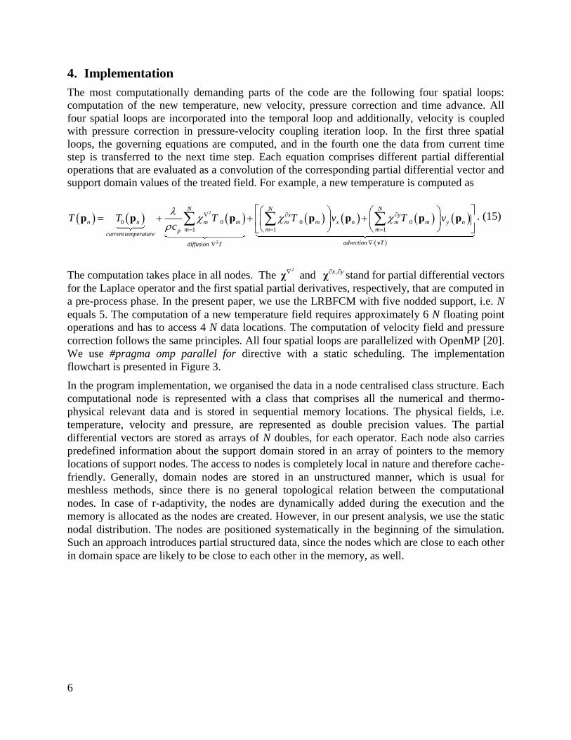
All tests are performed on a computer system with four Intel Xeon E4870 processors with

Nehalem microarchitecture, each with ten cores, system clock of 2.80 GHz, 3200 MHz front side

bus (FSB), and 64 GB of shared main memory. The system has three levels of cache hierarchy:

each core has 32 kB of L1 instruction cache and 32 kB of L1 data cache, 256 kB of L2 cache,

and shares 30 MB of L3 cache with the other cores of the processor. The latencies for accessing

data are 4 clock cycles for the L1 cache, typical 10 clock cycles for the L2 cache, 40 clock cycles

for the L3 cache, and an order 120 clock cycles for main memory [33]. The computer

architecture is schematically presented in Figure 4.

8

Figure 4: Scheme of the computer architecture used for the test case.

The tests are run on Nehalem microarchitecture; however, the results are not limited to a specific

architecture and thus a similar behaviour is expected on all current and future NUMA multicore

platforms.

5. Results

5.1. Results of numerical integration

The classical de Vahl Davis benchmark test is defined for the natural convection of the air

Pr 0.71 in a square closed cavity. The only free parameter of the test remains the thermal

Rayleigh number. In the original paper [21], de Vahl Davis tested the problem with the Rayleigh

number up to 610 . However, in the latest publications, the results of more intense simulations

were presented with the Rayleigh number up to 810 . Lage and Bejan [34] showed that the

laminar domain of the closed cavity natural convection problem is roughly below 9Gr<10 . It was

reported [35] that the natural convection becomes unsteady for 8Ra 2 10 . In this paper, we

deal with the steady solution and therefore, according to the published data, a case with the

maximum 8Ra 10 is considered. A detailed comparison of the presented numerical approach

against previously published data has been already done in [32], where the range of 3 8Ra 10 ,10

has been analysed. It has been shown that the proposed local approach is in a

good agreement with the previous work, as well as convergent, conservative and stable [32]. The

presented solution procedure has been also successfully applied on several other thermo-fluid

problems, where the latest and also the most complex simulation was solidification of a binary

alloy [25]. The published tests confirm that the presented meshless numerical solution procedure

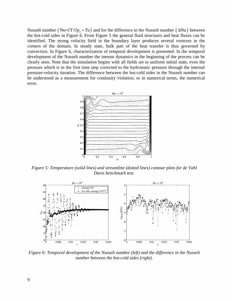
provides good results. In Figure 5 the results for 8Ra 10 case are presented in terms of the

stream function and temperature contour plot. Note that all results are stated in the standard

dimensionless form. Additional results are presented in terms of temporal development of the

9

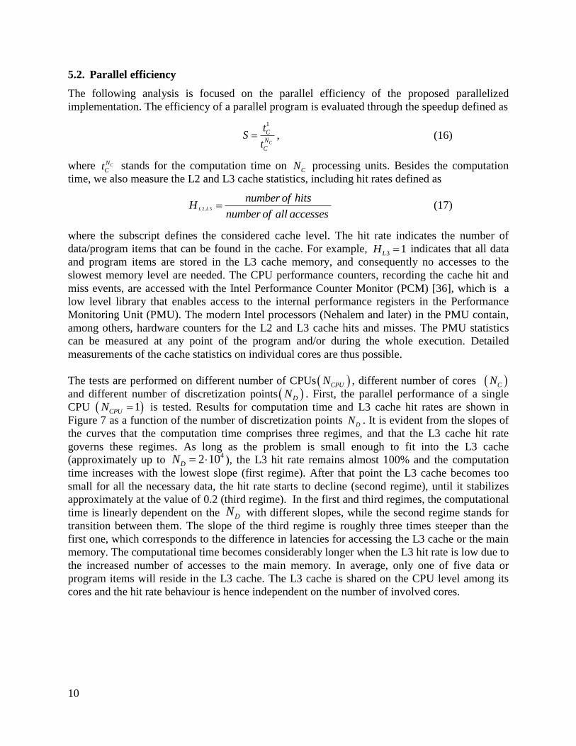
Nusselt number Nu= / xT p Tu and for the difference in the Nusselt number Nu between

the hot-cold sides in Figure 6. From Figure 5 the general fluid structures and heat fluxes can be

identified. The strong velocity field in the boundary layer produces several vortexes in the

corners of the domain. In steady state, bulk part of the heat transfer is thus governed by

convection. In Figure 6, characterization of temporal development is presented. In the temporal

development of the Nusselt number the intense dynamics in the beginning of the process can be

clearly seen. Note that the simulation begins with all fields set to uniform initial state, even the

pressure which is in the first time step corrected to the hydrostatic pressure through the internal

pressure-velocity iteration. The difference between the hot-cold sides in the Nusselt number can

be understood as a measurement for continuity violation, or in numerical terms, the numerical

error.

Figure 5: Temperature (solid lines) and streamline (dotted lines) contour plots for de Vahl

Davis benchmark test.

Figure 6: Temporal development of the Nusselt number (left) and the difference in the Nusselt

number between the hot-cold sides (right).

10

5.2. Parallel efficiency

The following analysis is focused on the parallel efficiency of the proposed parallelized

implementation. The efficiency of a parallel program is evaluated through the speedup defined as

1

C

C

N

C

tS

t , (16)

where CN

Ct stands for the computation time on CN processing units. Besides the computation

time, we also measure the L2 and L3 cache statistics, including hit rates defined as

2, 3L L

number of hitsH

number of all accesses (17)

where the subscript defines the considered cache level. The hit rate indicates the number of

data/program items that can be found in the cache. For example, 3 1LH indicates that all data

and program items are stored in the L3 cache memory, and consequently no accesses to the

slowest memory level are needed. The CPU performance counters, recording the cache hit and

miss events, are accessed with the Intel Performance Counter Monitor (PCM) [36], which is a

low level library that enables access to the internal performance registers in the Performance

Monitoring Unit (PMU). The modern Intel processors (Nehalem and later) in the PMU contain,

among others, hardware counters for the L2 and L3 cache hits and misses. The PMU statistics

can be measured at any point of the program and/or during the whole execution. Detailed

measurements of the cache statistics on individual cores are thus possible.

The tests are performed on different number of CPUs CPUN , different number of cores CN

and different number of discretization points DN . First, the parallel performance of a single

CPU 1CPUN is tested. Results for computation time and L3 cache hit rates are shown in

Figure 7 as a function of the number of discretization points DN . It is evident from the slopes of

the curves that the computation time comprises three regimes, and that the L3 cache hit rate

governs these regimes. As long as the problem is small enough to fit into the L3 cache

(approximately up to 42 10DN ), the L3 hit rate remains almost 100% and the computation

time increases with the lowest slope (first regime). After that point the L3 cache becomes too

small for all the necessary data, the hit rate starts to decline (second regime), until it stabilizes

approximately at the value of 0.2 (third regime). In the first and third regimes, the computational

time is linearly dependent on the DN with different slopes, while the second regime stands for

transition between them. The slope of the third regime is roughly three times steeper than the

first one, which corresponds to the difference in latencies for accessing the L3 cache or the main

memory. The computational time becomes considerably longer when the L3 hit rate is low due to

the increased number of accesses to the main memory. In average, only one of five data or

program items will reside in the L3 cache. The L3 cache is shared on the CPU level among its

cores and the hit rate behaviour is hence independent on the number of involved cores.

11

Figure 7: Computation time (left) and L3 cache hit rate (right) with the respect to the number

of discretization points and the number of cores on a single CPU.

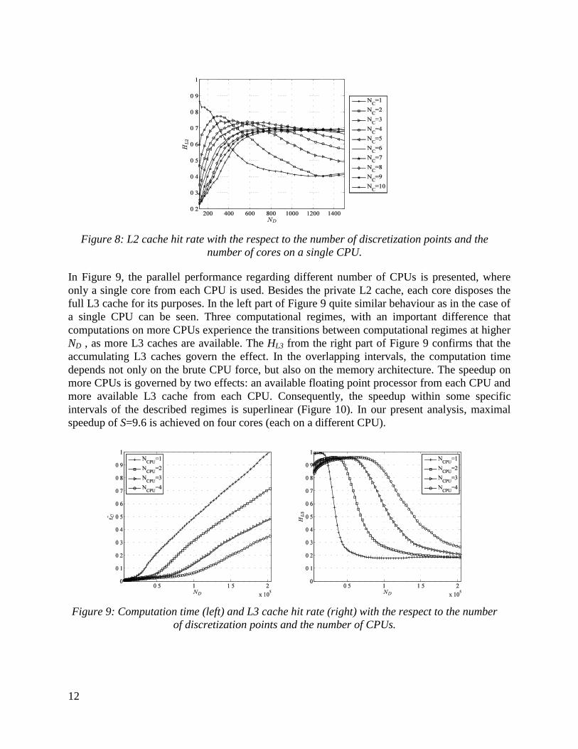
Next analysis is focused on the impact of the L2 cache on the computation performance on a

single CPU. The L2 hit rate results are shown in Figure 8. The variations in2LH have been

significantly larger than in the L3 cache as the L2 cache is much smaller and therefore more

dependent on the cache policies and operating system tasks. Also, the DN

range of the visible L2

cache impact is much smaller than of the L3. The 2LH also depends on the number of cores

since the L2 caches are private in each core. For better presentation of the main findings, the L2

measurements are smoothed with a low pass filter. From Figure 8, it is visible that for small ND

the hit rate of a single core is much higher than the hit rate of multicore computations. Small

systems fit into the L2 cache, and as long as only a single core is used, there is no

communication between cores and thus virtually no cache misses. In the case with more cores

used, each time a core modifies a memory location on its local cache, it invalidates the caches on

other cores that occupy the same memory location. While this frequently happens on shared data,

it also happens on private data, because multiple variables might inhabit the same cache block. In

our test case, such behaviour is frequent since variables written by one core are interleaved with

variables read by another core. Invalidation of L2 cache blocks introduces L2 cache misses and

consequently L3 cache accesses. The described invalidation effect is amplified with the number

of cooperating cores. By increased problem size, HL2 converges approximately to the value of

0.5. For a single core, the saturation is achieved approximately after ND = 600 discretization

points, while for higher number of cores this limit increases. As long as theDN is small and all

the data fits into one L2 cache, the invalidation effect is strong; however, when the dataset

becomes bigger, the accumulating L2 caches improves the computation performance. The

interplay of those two effects is clearly demonstrated on Figure 8. Nevertheless, for complex

computations, the memory demands are much bigger than the size of the L2 cache.

12

Figure 8: L2 cache hit rate with the respect to the number of discretization points and the

number of cores on a single CPU.

In Figure 9, the parallel performance regarding different number of CPUs is presented, where

only a single core from each CPU is used. Besides the private L2 cache, each core disposes the

full L3 cache for its purposes. In the left part of Figure 9 quite similar behaviour as in the case of

a single CPU can be seen. Three computational regimes, with an important difference that

computations on more CPUs experience the transitions between computational regimes at higher

ND , as more L3 caches are available. The HL3 from the right part of Figure 9 confirms that the

accumulating L3 caches govern the effect. In the overlapping intervals, the computation time

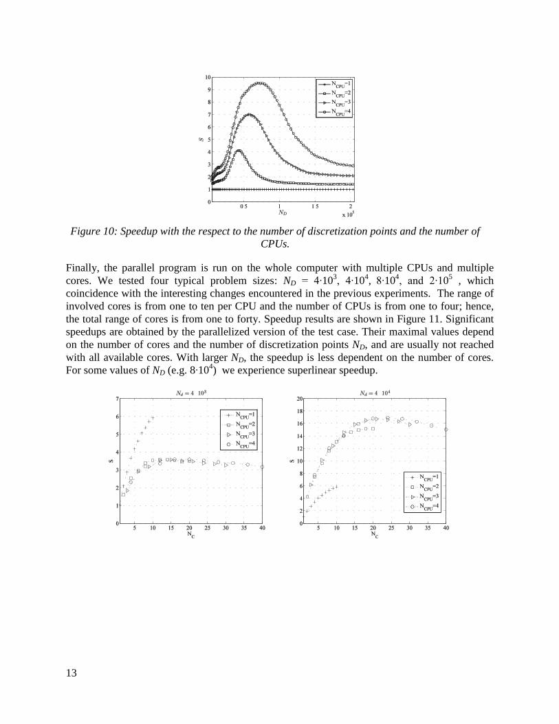
depends not only on the brute CPU force, but also on the memory architecture. The speedup on

more CPUs is governed by two effects: an available floating point processor from each CPU and

more available L3 cache from each CPU. Consequently, the speedup within some specific

intervals of the described regimes is superlinear (Figure 10). In our present analysis, maximal

speedup of S=9.6 is achieved on four cores (each on a different CPU).

Figure 9: Computation time (left) and L3 cache hit rate (right) with the respect to the number

of discretization points and the number of CPUs.

13

Figure 10: Speedup with the respect to the number of discretization points and the number of

CPUs.

Finally, the parallel program is run on the whole computer with multiple CPUs and multiple

cores. We tested four typical problem sizes: ND = 4∙103, 4∙10

4, 8∙10

4, and 2∙10

5 , which

coincidence with the interesting changes encountered in the previous experiments. The range of

involved cores is from one to ten per CPU and the number of CPUs is from one to four; hence,

the total range of cores is from one to forty. Speedup results are shown in Figure 11. Significant

speedups are obtained by the parallelized version of the test case. Their maximal values depend

on the number of cores and the number of discretization points ND, and are usually not reached

with all available cores. With larger ND, the speedup is less dependent on the number of cores.

For some values of ND (e.g. 8∙104) we experience superlinear speedup.

14

Figure 11: Speedup for different number of discretization points with respect to the number of

cores and the number of CPUs.

6. Discussion

In the present paper, we analyse the behaviour of parallelized implementation of the strong form

LRBFCM in solving thermo-fluid problems. In contrast to conventional numerical methods, the

LBRFCM relays on local meshless technique with several degrees of freedom in the type of

approximation [23, 37], in the selection of basis and its augmentation [38], conditioning [39] and

optimized weighting [40] of the approximation, in distribution of discretization nodes [41], in the

size of the local support domains [37, 42], etc. The advanced usage of meshless methods can be

applied to treat numerical anomalies or cases where special treatment is required. The method

can be severely altered by changing only its parameters, which can be done on the fly during the

simulation. For example, in the case of shockwave propagation, the r-adaptation can be easily

applied [29] to ease the numerical instabilities without introducing additional numerical

dissipation. Convective dominated problems can be also treated with the adaptive upwind [43]

that uses local Péclét number to evaluate the magnitude and the direction of the upwind offset.

All these features are inherent in meshless and do not require any kind of special treatment of the

numerical algorithms and the code. On the other hand, the local differential vector formulation

simplifies the implementation and the understanding of the method to the level of FDM, but still

conserves all the mentioned advantages.

An evident drawback of the meshless could be the higher complexity because of the additional

effort needed to maintain the support domain nodes. However, specialized data structures are

known, e.g. KD tree [12], that enable efficient searching of support nodes in logD DO N N time

and can be also done in a pre-process and/or only when the nodal topology changes. The number

of support nodes might be also higher than in conventional approaches. For example, central

FDM scheme requires only five nodes in 2D, while Diffuse Approximate Method based on

Weighted Least Squares approximation requires 13 support nodes [37]. The LBRFCM method is

based on collocation and typically requires less support nodes in the support domain. In our

implementation, we use the smallest possible setup of 5N , which implies that its

computational complexity is in the order of DO N N and is comparable to the one of FDM. The

memory complexity of LRBFCM is however higher in comparison to the FDM. The LRBFCM

does not require any kind of topological relations between nodes and consequently the partial

15

differentials are spatial dependent; the memory complexity is therefore DO N N , while for

FDM only O N .

A further drawback of the LBRFCM method could be the lower accuracy, in particular, in some

inconvenient distribution of local nodes [44], which could happen for larger DN . However, it has

been shown in [45] and with extensive experimental results in [12, 22] that the local strong form

meshless formulation provides results comparable to the weak formulated Meshless Local Petrov

Galerkin Method (MLPG) and FEM on structured and non-structured discretization nodes. It was

also confirmed in [46] that the local formulation of LRBFCM outperforms the global approach

significantly in larger systems, which equates the LBRFCM with conventional strong formulated

methods.

The experimental results presented in our paper are used for the analysis and prediction of the

execution performances in different application regimes. Regarding the execution speedup,

superlinear regimes are identified, governed by the accumulated L3 caches. Detailed analysis of

the parallel program execution time reveals that the superlinear regime occurs as a consequence

of accumulating L3 caches. This conclusion is supported by the evaluation of the CPU

performance through measured memory cache statistics from PMU. The measurements

confirmed the theoretical expectations and explain the superlinearity with the maximum of S =

9.6 on 4 cores. Based on the presented results, some clear and generally applicable conclusions

can be drawn. As long as the size of the problem is small (below 104 in our test case) and all the

data fits into a single L3 cache, it is beneficial to use multiple cores on a single CPU for

improved speedup. Using more CPUs in that case would introduce communication between the

CPUs, which lowers the speedup. In larger problems (between 104 and 10

5), the accumulated L3

caches may produce superlinear speedups using more CPUs with only a single core from each.

The maximal size of the problem, which still provides superlinearity, depends on the memory

architecture. However, L3 caches are in general relatively big and thus, the effect should be

detectable on most of the modern computer systems. The largest problems (above 105) that do

not fit into accumulated L3 caches will be executed in the shortest time if all available CPUs and

cores are exploited. However, there is a maximal speedup that cannot be exceeded, because it is

limited by the bandwidth of the main memory.

Our discussion will finally touch a prediction for the expected speedup behaviour in the case of

other well established solution approaches, in particular, weak formulated Galerkin methods with

the main representatives FEM and meshless MLPG. It is known from the analysis published in

[12] that the complexities of the final system construction for these methods are D qO N n and

2logD q DO N n N Nm , respectively, where qn is the number of integration points and m is

the number of monomial basis functions. It follows that the weak formulated methods are in

general more complex because of numerical integration of the weak form, which requires

additional evaluation of the trial function in the integration points. Additionally, MLPG is an

approximation method that requires at least 11 nodes in the support domain and inherits all

problems with maintaining the support nodes in a specialized data structure. We can expect an

increased complexity of the Galerkin methods for a factor of qn , regarding the number of

floating point operations, and the same memory complexity, because numerical integration will

not require additional storage.

16

7. Conclusions

An OpenMP based parallel implementation of a strong formulated local meshless procedure

LBRFCM for solving fluid flow problems is demonstrated on an off-the-shelf computer server

with 4 CPUs, each with 10 cores. The standard de Vahl Davis natural convection test is used for

benchmarking purposes. It is shown that one can efficiently solve non-linear coupled problems,

like the natural convection fluid flow problem, with LBRFCM, which offers several convenient

features, such as the ease of implementation, adequate stability, accuracy, and convergence. The

methodology also offers several degrees of freedom for altering in order to treat anomalies or

special numerical cases. We confirmed that the parallelization of the LBRFCM is

straightforward on shared-memory systems. A minor amount of effort and expertise are required

to parallelize the sequential code, thus the approach is interesting for engineering computations.

It is demonstrated through extensive experiments that the efficiency of the parallel

implementation is gravely affected by the memory architecture of the computational system. A

significant speedup in the execution can be achieved if appropriate architecture is used for a

specific problem size. The effect is explained by on-line measurements of memory cache

statistics with the Performance Monitoring Units of the CPUs. It is shown that accumulating L3

caches govern the effect. In other words, it is not only the computational power of the CPU that

matters in intense simulations; memory access and communication speed are equally important.

There are still several factors that have not been explored in full details, e.g. motherboard

architecture, bandwidths of data and program buses, cache policies, etc. They could influence the

results but do not change the main findings. Future work is focused on more detailed analysis of

new architecture-dependant factors and application of the proposed methodology in realistic

technological processes and 3D structures.

Acknowledgment

We acknowledge the financial support from the state budget by the Slovenian Research Agency

under the grants P2-0095, PR-03266 and J2-4120.

8. References

[1] Ferziger JH, Perić M. Computational Methods for Fluid Dynamics. Berlin: Springer; 2002.

[2] Őzisik MN. Finite Difference Methods in Heat Transfer. Boca Raton: CRC Press; 2000.

[3] Wrobel LC. The Boundary Element Method: Applications in Thermo-Fluids and Acoustics.

West Sussex: John Wiley & Sons; 2002.

[4] Rappaz M, Bellet M, Deville M. Numerical Modelling in Materials Science and Engineering.

Berlin: Springer-Verlag; 2003.

[5] Atluri SN, Shen S. The Meshless Method. Encino: Tech Science Press; 2002.

[6] Liu GR, Gu YT. An Introduction to Meshfree Methods and Their Programming. Dordrecht:

Springer; 2005.

[7] Nguyen VP, Rabczuk T, Bordas S, Duflot M. Meshless methods: A review and computer

implementation aspects. Mathematics and Computers in Simulation. 2008;79:763-813.

[8] Mirzaei D, Schaback R. Direct Meshless Local Petrov-Galerkin (DMLPG) method: A

generalized MLS approximation. Appl Numer Math. 2013;68:73-82.

17

[9] Wang JG, Liu GR. A point interpolation meshless method based on radial basis functions. Int

J Numer Meth Eng. 2002;54:1623-48.

[10] Šarler B, Perko J, Chen CS. Radial basis function collocation method solution of natural

convection in porous Media. Int J Numer Method H. 2004;14:187-212.

[11] Kansa EJ. Multiquadrics - a scattered data approximation scheme with application to

computational fluid dynamics, part I. Comput Math Appl. 1990;19:127-45.

[12] Trobec R, Šterk M, Robič B. Computational complexity and parallelization of the meshless

local Petrov-Galerkin method. Comput Struct. 2009;87:81-90.

[13] Pacheco PS. An Introduction to Parallel Programming. Burlington: Morgan Kaufmann

Publishers; 2011.

[14] Kirk DB, Hwu WW. Programming Massively Parallel Processors. Burlington: Morgan

Kaufmann Publishers; 2010.

[15] Domínguez JM, Crespo AJC, Valdez-Balderas D, Rogers BD, Gómez-Gesteira M. New

multi-GPU implementation for smoothed particle hydrodynamics on heterogeneous clusters.

Comput Phys Commun. 2013.

[16] Singh V. Parallel implementation of the EFG Method for heat transfer and fluid flow

problems. Comput Mech. 2004;34:453–63.

[17] Zhang L, Wagner GJ, Liu WK. A parallelized meshfree method with boundary enrichment

for large-scale CFD. J Comput Phys. 2002;176:483–506.

[18] Rabczuk T, Bordas S, Askes H. Meshfree Methods for Dynamic Fracture. Computational

Technology Reviews. 2010;1:157-85.

[19] Venkatesh TN, Sarasamma VR, Rajalakshmy, Kirti Chandra Sahu S, Govindarajan R.

Super-linear speed-up of a parallel multigrid navier-stokes solver on flosolver. Ecol Ec Env.

2005;88:589-93.

[20] Chandra R, Dagum L, Kohr D, Maydan D, McDonald J, Menon R. Parallel Programming in

OpenMP. San Diego: Academic Press; 2001.

[21] de Vahl Davis G. Natural convection of air in a square cavity: a bench mark numerical

solution. Int J Numer Meth Fl. 1983;3:249-64.

[22] Trobec R, Kosec G, Šterk M, Šarler B. Comparison of local weak and strong form meshless

methods for 2-D diffusion equation. Eng Anal Bound Elem. 2012;36:310-21.

[23] Vertnik R, Šarler B. Meshless local radial basis function collocation method for convective-

diffusive solid-liquid phase change problems. Int J Numer Method H. 2006;16:617-40.

[24] Divo E, Kassab AJ. Localized meshless modeling of natural-convective viscous flows.

Numer Heat Transfer. 2007;B129:486-509.

[25] Kosec G, Založnik M, Šarler B, Combeau H. A Meshless Approach Towards Solution of

Macrosegregation Phenomena. CMC-Comput Mater Con. 2011;580:1-27.

[26] Prax C, Sadat H, Salagnac P. Diffuse approximation method for solving natural convection

in porous Media. Theor App T. 1996;22:215-23.

[27] Wan DC, Patnaik BSV, Wei GW. A new benchmark quality solution for the buoyancy-

driven cavity by discrete singular convolution. Numer Heat Transfer. 2001;B40:199-228.

[28] Franke J. Scattered data interpolation: tests of some methods. Math Comput. 1982;48:181-

200.

[29] Kosec G, Šarler B. H-adaptive local radial basis function collocation meshless method.

CMC-Comput Mater Con. 2011;26:227-53.

18

[30] Malan AG, Lewis RW. An artificial compressibility CBS method for modelling heat

transfer and fluid flow in heterogeneous porous materials. Int J Numer Meth Eng. 2011;87:412-

23.

[31] Hong CP. Computer Modelling of Heat and Fluid Flow Materials Processing. Bristol:

Institute of Physics Publishing; 2004.

[32] Kosec G, Šarler B. Solution of thermo-fluid problems by collocation with local pressure

correction. Int J Numer Method H. 2008;18:868-82.

[33] INTEL. 64 and IA-32 Architectures Optimization Reference Manual.

http://www.intel.com/content/www/us/en/architecture-and-technology/64-ia-32-architectures-

optimization-manual.html.

[34] Lage JL, Bejan A. The Ra-Pr domain of laminar natural convection in an enclosure heated

from the side. Numer Heat Transfer. 1991;A19:21-41.

[35] Nobile E. Simulation of time-dependent flow in cavities with the additive-correction

multigrid method, part II: Apllications. Numer Heat Transfer. 1996;B30:341-50.

[36] INTEL. Performance Counter Monitor. http://software.intel.com/en-us/articles/intel-

performance-counter-monitor.

[37] Prax C, Sadat H, Dabboura E. Evaluation of high order versions of the diffuse approximate

meshless method. Appl Math Comput. 2007;186:1040–53.

[38] Zhang Y, Sim T, Tan CL, Sung E. Anatomy-based face reconstruction for animation using

multi-layer deformation. J Visual Lang Comput. 2006;17:126-60.

[39] Lee CK, Liu X, Fan SC. Local muliquadric approximation for solving boundary value

problems. Comput Mech. 2003;30:395-409.

[40] Perko J, Šarler B. Weigh function shape parameter optimization in meshless methods for

non-uniform grids. CMES-Comp Model Eng. 2007;19:55-68.

[41] Kovačević I, Šarler B. Solution of a phase-field model for dissolution of primary particles in

binary aluminum alloys by an r-adaptive mesh-free method. Mater Sci Eng. 2005;A413-414:423-

8.

[42] Šarler B, Vertnik R. Meshfree explicit local radial basis function collocation method for

diffusion problems. Comput Math Appl. 2006;51:1269-82.

[43] Lin H, Atluri SN. Meshless local Petrov Galerkin method (MLPG) for convection-diffusion

problems. CMES-Comp Model Eng. 2000;1:45-60.

[44] Šterk M, Trobec R. Meshless solution of a diffusion equation with parameter optimization

and error analysis. Eng Anal Bound Elem. 2008;32:567-77.

[45] Wang CA, Sadat H, Prax C. A new meshless approach for three dimensional fluid flow and

related heat transfer problems. Computers and Fluids. 2012;69:136-46.

[46] Yao G, Šarler B. Assessment of global and local meshless methods based on collocation

with radial basis functions for parabolic partial differential equations in three dimensions. Eng

Anal Bound Elem. 2012;36:1640-8.