Super-Gaussian Transport Theory and Field Generating Instability in Laser-Plasmas

J. J. Bissell and R. J. Kingham Blackett Laboratory Imperial College London SW7 2BZ

1 Introduction Accurate prediction of plasma transport is essential to the success of long-pulse (100ps-10ns) experiments, such as those at the National Ignition Facility in the United States.i Transport is commonly modelled using magnetohydrodynamics (MHD) - an approach based on the fluid equations and closed using Braginskii's classical transport theory, i.e., assuming that the electron distribution function is close to a Gaussian.ii,iii,iv However, for laser intensities in the range 1014-1015Wcm-2

(typical of long-pulse experiments), heating is dominated by inverse bremsstrahlung, and this mechanism tends to distort the distribution function away from a Gaussian by preferentially transmitting energy to slower, more collisional electrons. In fact, the distribution function f0 tends to a super-Gaussian; that is, f0(v)exp[-(v/evT)m], where v is the electron velocity, m[2,5], e is a function of m, and vT=(2Te/me)1/2 is the thermal velocity, with Te and me as the electron temperature and mass respectively.v,vi Notice that when m=2 we recover the usual Gaussian form. The super-Gaussian power m is calculated from the ion atomic number Z and the electron quiver velocity vosc. using the formula of Matte et al.,vi

m 2 311.66 /aM

0.724 , where aM Z(vosc. /vT )2 . (1)

Recently, Ridgers et al. have shown that a super-Gaussian may be used as the basis for re-deriving the transport theory, and gave expressions for the electric field E and heat-flow q to account for I.B. effects in fluid codes, thus mitigating the need for expensive kinetic calculations.vii Ridgers's modified transport equations are

eneE c Pe jB me

e B

c j nec Te

(2)

and

q ne BTe

me

c Te 'j Te

e BTe

me

c Pe ,

(3)

where e is the electronic charge, ne is the electron number density, Pe=neTe is the isotropic pressure, j is the current, B is the magnetic field flux-density and B=cBT is the Braginkii collision time, which is proportional to the thermal collision time T=(4vT

3)/(ni[Ze2/0me]2logei) by the factor cB =31/2/4, where ni is the ion number density, 0 is the permittivity of free space and logei8 is the Coulomb logarithm. Ridgers used the Lorentz approximation, so the transport coefficients c, c, c, c=('-[5/2]I), c and c are dimensionless functions of both m and the Hall Parameter =LB only, where L=(e|B|/me) is the electron thermal Larmor frequency.vii Note that classical transport theory, for which c=c and c=c=I (the identity tensor), is recovered when m=2. The resistivity c, conductivity c, and thermoelectric tensors c and c may thus be termed `old' coefficients, whose values are modified depending on the super-Gaussian power m, while c and c are `new' coefficients describing novel I.B. effects. The magnetic field provides a natural reference direction for the transport so that a general

coefficient may be written in terms of three components , || and , viz

||b(b s) b (s b) b s, (4)

where b=B/|B| is a unit vector in the direction of the magnetic field and s is the driving force behind the transport. Convention dictates that in the case of the resistivity c, for which the driving force is s=j, the final term in this expression takes a negative rather than positive sign. Note that only the components are unique , because ||=(=0).iii,iv,vii

Ridgers demonstrated the applicability of the super-Gaussian transport theory, and noted modifications to the `old' coefficients; however, he did not consider the implications of the new terms.vii Consequently, the first part of this report is devoted to an exploration of some of the ways super-Gaussians might be expected to modify transport in magnetized plasmas. We shall show that the addition of `new' coefficients has two principle consequences: first, the suppression of traditional transport phenomena; and second, the introduction of new effects. Indeed, we shall demonstrate that transport is strongly affected by super-Gaussian effects in the limit of low , suggesting that the theory may be most relevant to the seeding and evolution of magnetic fields in otherwise un-magnetized conditions. For this reason, later sections are devoted to a discussion of its consequences for the well-known field generating thermal instability.viii,ix,x

2 Super-Gaussian Effects in the Induction Equation Using the chain rule to write Pe=neTe+Tene, the consequences of the c coefficient may be considered by looking at its contribution to the induction equation, found after substituting equation (2) into Faraday's Law, i.e.,

Bt

E

Te

c

ene

ne jB me

c

e2ne B

j c c Te

e

.

(5)

The final term in this equation represents the Nernst effect,xi that is, advection of the magnetic field down temperature gradients. Retaining just this term, applying the expansion of equation (4), and keeping only the cross-field parts, we find

Bt

(vN B), where vN cB

2T

2

B

( )Te

Te

(6)

is the Nernst advection velocity and T=vTT is the thermal mean-free-path (c.f. A. Nishiguchi et al.xi). The coefficient (which is positive) is reduced in the super-Gaussian theory; however, because is negative, the Nernst velocity is further suppressed by the new coefficient. Indeed, for the case where m=5, when is of a similar order to , we see as much as a five-fold reduction in the Nernst velocity vN in the low χ limit (see figure 1).

Contact j.bissell07@imperial.ac.uk

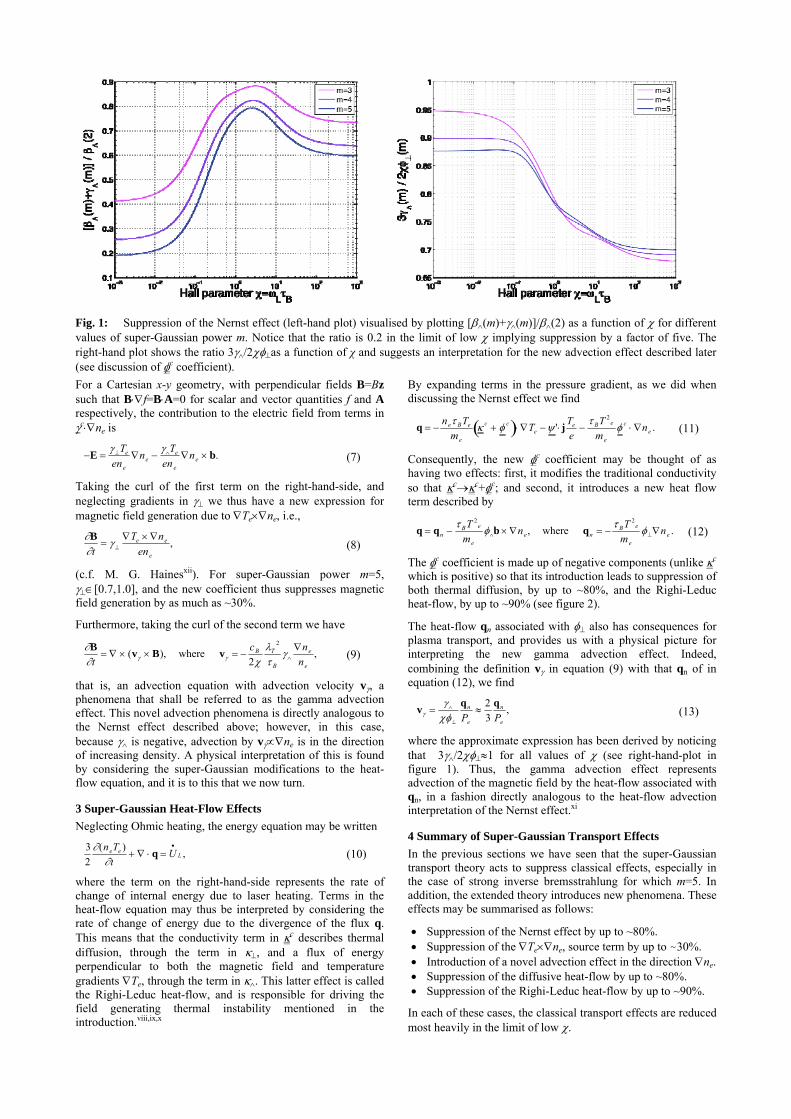
Fig. 1: Suppression of the Nernst effect (left-hand plot) visualised by plotting [(m)+(m)]/(2) as a function of for different values of super-Gaussian power m. Notice that the ratio is 0.2 in the limit of low implying suppression by a factor of five. The right-hand plot shows the ratio 3/2as a function of χ and suggests an interpretation for the new advection effect described later (see discussion of c coefficient). For a Cartesian x-y geometry, with perpendicular fields B=Bz such that Bf=BA=0 for scalar and vector quantities f and A respectively, the contribution to the electric field from terms in cne is

E Te

ene

ne Te

ene

ne b. (7)

Taking the curl of the first term on the right-hand-side, and neglecting gradients in we thus have a new expression for magnetic field generation due to Tene, i.e.,

Bt

Te ne

ene

, (8)

(c.f. M. G. Hainesxii). For super-Gaussian power m=5, [0.7,1.0], and the new coefficient thus suppresses magnetic field generation by as much as ~30%.

Furthermore, taking the curl of the second term we have

Bt

(v B), where v cB

2T

2

B

ne

ne

, (9)

that is, an advection equation with advection velocity v, a phenomena that shall be referred to as the gamma advection effect. This novel advection phenomena is directly analogous to the Nernst effect described above; however, in this case, because is negative, advection by vne is in the direction of increasing density. A physical interpretation of this is found by considering the super-Gaussian modifications to the heat-flow equation, and it is to this that we now turn.

3 Super-Gaussian Heat-Flow Effects Neglecting Ohmic heating, the energy equation may be written

32(neTe )

t q U

L , (10)

where the term on the right-hand-side represents the rate of change of internal energy due to laser heating. Terms in the heat-flow equation may thus be interpreted by considering the rate of change of energy due to the divergence of the flux q. This means that the conductivity term in c describes thermal diffusion, through the term in , and a flux of energy perpendicular to both the magnetic field and temperature gradients Te, through the term in . This latter effect is called the Righi-Leduc heat-flow, and is responsible for driving the field generating thermal instability mentioned in the introduction.viii,ix,x

By expanding terms in the pressure gradient, as we did when discussing the Nernst effect we find

q ne BTe

me

c c Te ' j Te

e BT 2

e

me

c ne . (11)

Consequently, the new c coefficient may be thought of as having two effects: first, it modifies the traditional conductivity so that cc+c; and second, it introduces a new heat flow term described by

q qn BT 2

e

me

b ne , where qn BT 2

e

me

ne . (12)

The c coefficient is made up of negative components (unlike c which is positive) so that its introduction leads to suppression of both thermal diffusion, by up to ~80%, and the Righi-Leduc heat-flow, by up to ~90% (see figure 2).

The heat-flow qn associated with also has consequences for plasma transport, and provides us with a physical picture for interpreting the new gamma advection effect. Indeed, combining the definition v in equation (9) with that qn of in equation (12), we find

v

qn

Pe

23

qn

Pe

, (13)

where the approximate expression has been derived by noticing that 3/21 for all values of (see right-hand-plot in figure 1). Thus, the gamma advection effect represents advection of the magnetic field by the heat-flow associated with qn, in a fashion directly analogous to the heat-flow advection interpretation of the Nernst effect.xi

4 Summary of Super-Gaussian Transport Effects In the previous sections we have seen that the super-Gaussian transport theory acts to suppress classical effects, especially in the case of strong inverse bremsstrahlung for which m=5. In addition, the extended theory introduces new phenomena. These effects may be summarised as follows:

Suppression of the Nernst effect by up to ~80%. Suppression of the Tene, source term by up to ~30%. Introduction of a novel advection effect in the direction ne. Suppression of the diffusive heat-flow by up to ~80%. Suppression of the Righi-Leduc heat-flow by up to ~90%.

In each of these cases, the classical transport effects are reduced most heavily in the limit of low .

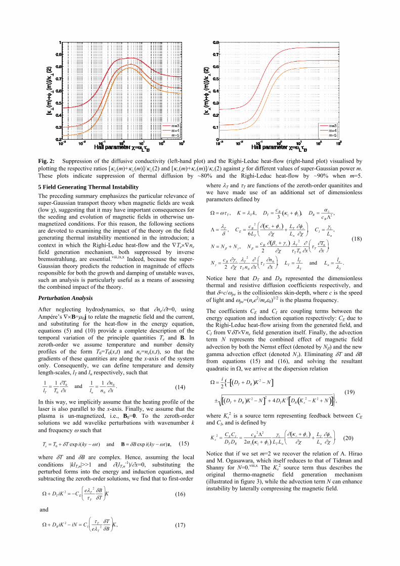
Fig. 2: Suppression of the diffusive conductivity (left-hand plot) and the Righi-Leduc heat-flow (right-hand plot) visualised by plotting the respective ratios [(m)+(m)]/(2) and [(m)+(m)]/(2) against χ for different values of super-Gaussian power m. These plots indicate suppression of thermal diffusion by ~80% and the Righi-Leduc heat-flow by ~90% when m=5.

5 Field Generating Thermal Instability The preceding summary emphasizes the particular relevance of super-Gaussian transport theory when magnetic fields are weak (low χ), suggesting that it may have important consequences for the seeding and evolution of magnetic fields in otherwise un-magnetized conditions. For this reason, the following sections are devoted to examining the impact of the theory on the field generating thermal instability mentioned in the introducion; a context in which the Righi-Leduc heat-flow and the Tene field generation mechanism, both suppressed by inverse bremsstrahlung, are essential.viii,ix,x Indeed, because the super-Gaussian theory predicts the reduction in magnitude of effects responsible for both the growth and damping of unstable waves, such an analysis is particularly useful as a means of assessing the combined impact of the theory.

Perturbation Analysis

After neglecting hydrodynamics, so that ne/t=0, using Ampére’s B=0j to relate the magnetic field and the current, and substituting for the heat-flow in the energy equation, equations (5) and (10) provide a complete description of the temporal variation of the principle quantities Te and B. In zeroth-order we assume temperature and number density profiles of the form T0=T0(x,t) and ne=ne(x,t), so that the gradients of these quantities are along the x-axis of the system only. Consequently, we can define temperature and density length-scales, lT and ln respectively, such that

1lT

1T0

T0

xand 1

ln

1n0

n0

x. (14)

In this way, we implicitly assume that the heating profile of the laser is also parallel to the x-axis. Finally, we assume that the plasma is un-magnetized, i.e., B0=0. To the zeroth-order solutions we add wavelike perturbations with wavenumber k and frequency such that

Te T0 T exp i(ky t) and B B exp i(ky t)z, (15)

where T and B are complex. Hence, assuming the local conditions |klT,n|>>1 and (lT,n

-1)/x=0, substituting the perturbed forms into the energy and induction equations, and subtracting the zeroth-order solutions, we find that to first-order

DT iK 2 CE

eT2

T

B

T

K

(16)

and

DRiK 2 iN CI

T

eT2T

B

K , (17)

where T and T are functions of the zeroth-order quanitites and we have made use of an additional set of dimensionless parameters defined by

T , K T k, DT cB

3 || || , DR

||

cB2 ,

T

, CE

cB2

6LT

LT

Ln

, CI

||

Ln

,

N N N , N cB

2

T

2

T T0

x

T

T0

x

,

N cB

2

T2

T n0

x

T

n0

x

, LT

lTT

and Ln ln

T

.

(18)

Notice here that DT and DR represented the dimensionless thermal and resistive diffusion coefficients respectively, and that =c/pe is the collisionless skin-depth, where c is the speed of light and pe=(nee

2/me0)1/2 is the plasma frequency.

The coefficients CE and CI are coupling terms between the energy equation and induction equation respectively: CE due to the Righi-Leduc heat-flow arising from the generated field, and CI from Tne field generation itself. Finally, the advection term N represents the combined effect of magnetic field advection by both the Nernst effect (denoted by N) and the new gamma advection effect (denoted N). Eliminating T and B from equations (15) and (16), and solving the resultant quadratic in , we arrive at the dispersion relation

i2

DT DR K 2 N

DT DR K 2 N 2 4DT K 2 DR Ks2 K 2 N ,

(19)

where Ks2 is a source term representing feedback between CE

and CI, and is defined by

K s2

CECI

DT DR

cB

22

2 || || || ||

LT Ln

LT

Ln

.

(20)

Notice that if we set m=2 we recover the relation of A. Hirao and M. Ogasawara, which itself reduces to that of Tidman and Shanny for N=0.viii,x The Ks

2 source term thus describes the original thermo-magnetic field generation mechanism (illustrated in figure 3), while the advection term N can enhance instability by laterally compressing the magnetic field.

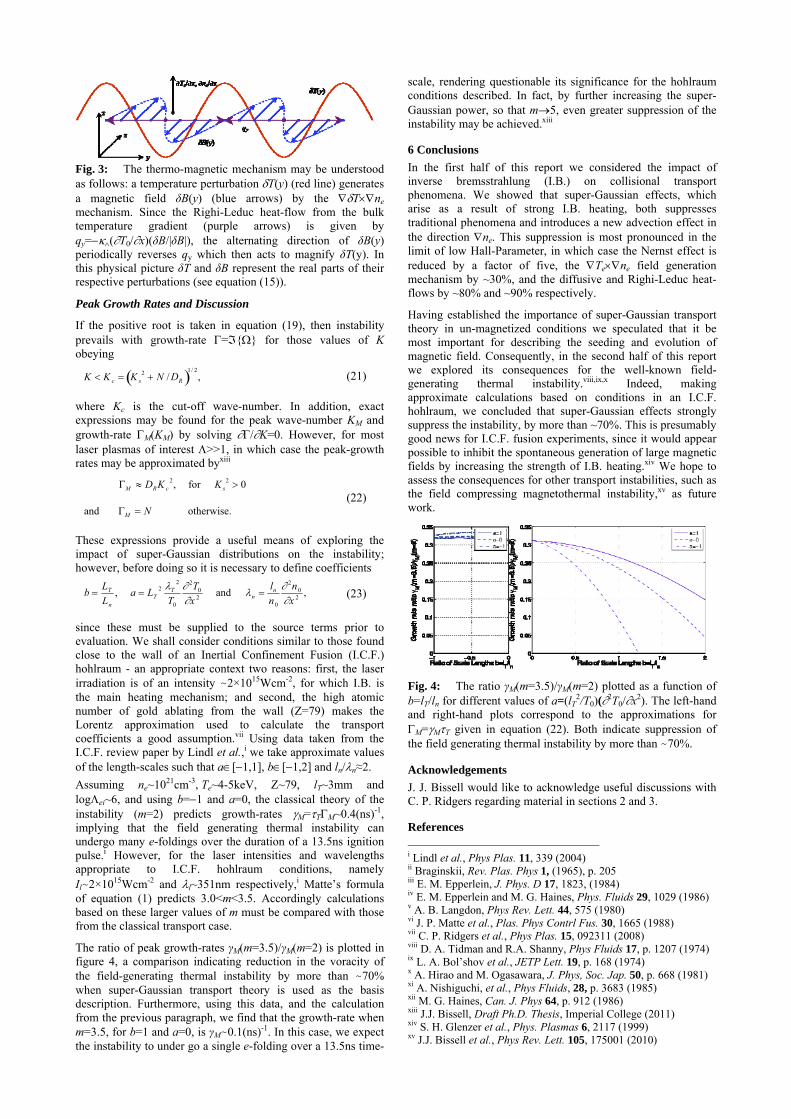
Fig. 3: The thermo-magnetic mechanism may be understood as follows: a temperature perturbation T(y) (red line) generates a magnetic field δB(y) (blue arrows) by the Tne mechanism. Since the Righi-Leduc heat-flow from the bulk temperature gradient (purple arrows) is given by qy=(T0/x)(δB/|δB|), the alternating direction of δB(y) periodically reverses qy which then acts to magnify δT(y). In this physical picture δT and δB represent the real parts of their respective perturbations (see equation (15)).

Peak Growth Rates and Discussion

If the positive root is taken in equation (19), then instability prevails with growth-rate = for those values of K obeying

K K c K s2 N /DR 1/ 2

, (21)

where Kc is the cut-off wave-number. In addition, exact expressions may be found for the peak wave-number KM and growth-rate M(KM) by solving /K=0. However, for most laser plasmas of interest >>1, in which case the peak-growth rates may be approximated byxiii

M DRK c2, for K s

2 0

and M N otherwise.

(22)

These expressions provide a useful means of exploring the impact of super-Gaussian distributions on the instability; however, before doing so it is necessary to define coefficients

b LT

Ln

, a LT2 T

2

T0

2T0

x 2 and n ln

n0

2n0

x 2 , (23)

since these must be supplied to the source terms prior to evaluation. We shall consider conditions similar to those found close to the wall of an Inertial Confinement Fusion (I.C.F.) hohlraum - an appropriate context two reasons: first, the laser irradiation is of an intensity ~2×1015Wcm-2, for which I.B. is the main heating mechanism; and second, the high atomic number of gold ablating from the wall (Z=79) makes the Lorentz approximation used to calculate the transport coefficients a good assumption.vii Using data taken from the I.C.F. review paper by Lindl et al.,i we take approximate values of the length-scales such that a[1,1], b[1,2] and ln/n≈2. Assuming ne~1021cm-3, Te~4-5keV, Z~79, lT~3mm and logei~6, and using b=1 and a=0, the classical theory of the instability (m=2) predicts growth-rates M=TM~0.4(ns)-1, implying that the field generating thermal instability can undergo many e-foldings over the duration of a 13.5ns ignition pulse.i However, for the laser intensities and wavelengths appropriate to I.C.F. hohlraum conditions, namely Il~2×1015Wcm-2 and l~351nm respectively,i Matte’s formula of equation (1) predicts 3.0<m<3.5. Accordingly calculations based on these larger values of m must be compared with those from the classical transport case.

The ratio of peak growth-rates γM(m=3.5)/γM(m=2) is plotted in figure 4, a comparison indicating reduction in the voracity of the field-generating thermal instability by more than ~70% when super-Gaussian transport theory is used as the basis description. Furthermore, using this data, and the calculation from the previous paragraph, we find that the growth-rate when m=3.5, for b=1 and a=0, is γM~0.1(ns)-1. In this case, we expect the instability to under go a single e-folding over a 13.5ns time-

scale, rendering questionable its significance for the hohlraum conditions described. In fact, by further increasing the super-Gaussian power, so that m5, even greater suppression of the instability may be achieved.xiii

6 Conclusions In the first half of this report we considered the impact of inverse bremsstrahlung (I.B.) on collisional transport phenomena. We showed that super-Gaussian effects, which arise as a result of strong I.B. heating, both suppresses traditional phenomena and introduces a new advection effect in the direction ne. This suppression is most pronounced in the limit of low Hall-Parameter, in which case the Nernst effect is reduced by a factor of five, the Tene field generation mechanism by ~30%, and the diffusive and Righi-Leduc heat-flows by ~80% and ~90% respectively.

Having established the importance of super-Gaussian transport theory in un-magnetized conditions we speculated that it be most important for describing the seeding and evolution of magnetic field. Consequently, in the second half of this report we explored its consequences for the well-known field-generating thermal instability.viii,ix,x Indeed, making approximate calculations based on conditions in an I.C.F. hohlraum, we concluded that super-Gaussian effects strongly suppress the instability, by more than ~70%. This is presumably good news for I.C.F. fusion experiments, since it would appear possible to inhibit the spontaneous generation of large magnetic fields by increasing the strength of I.B. heating.xiv We hope to assess the consequences for other transport instabilities, such as the field compressing magnetothermal instability,xv as future work.

Fig. 4: The ratio γM(m=3.5)/γM(m=2) plotted as a function of b=lT/ln for different values of a=(lT

2/T0)(2T0/x2). The left-hand and right-hand plots correspond to the approximations for M=MT given in equation (22). Both indicate suppression of the field generating thermal instability by more than ~70%.

Acknowledgements J. J. Bissell would like to acknowledge useful discussions with C. P. Ridgers regarding material in sections 2 and 3.

References i Lindl et al., Phys Plas. 11, 339 (2004) ii Braginskii, Rev. Plas. Phys 1, (1965), p. 205 iii E. M. Epperlein, J. Phys. D 17, 1823, (1984) iv E. M. Epperlein and M. G. Haines, Phys. Fluids 29, 1029 (1986) v A. B. Langdon, Phys Rev. Lett. 44, 575 (1980) vi J. P. Matte et al., Plas. Phys Contrl Fus. 30, 1665 (1988) vii C. P. Ridgers et al., Phys Plas. 15, 092311 (2008) viii D. A. Tidman and R.A. Shanny, Phys Fluids 17, p. 1207 (1974) ix L. A. Bol’shov et al., JETP Lett. 19, p. 168 (1974) x A. Hirao and M. Ogasawara, J. Phys, Soc. Jap. 50, p. 668 (1981) xi A. Nishiguchi, et al., Phys Fluids, 28, p. 3683 (1985) xii M. G. Haines, Can. J. Phys 64, p. 912 (1986) xiii J.J. Bissell, Draft Ph.D. Thesis, Imperial College (2011) xiv S. H. Glenzer et al., Phys. Plasmas 6, 2117 (1999) xv J.J. Bissell et al., Phys Rev. Lett. 105, 175001 (2010)

High-field electrodynamics in plasmasConta t d.burtonlan aster.a .ukDA BurtonDepartment of Physi s, Lan aster University& The Co k roft Institute, Daresbury, UK H WenDepartment of Physi s, Lan aster University& The Co k roft Institute, Daresbury, UKClassi al va uum Maxwellian ele trodynami s is alinear theory, and non-linearities arise only via the ou-pling of ele tromagneti elds and matter. Althoughnon-linear theories of ele trodynami s may be indu edfrom va uum persisten e amplitudes in QED [1, theorigin of the non-linearity may be understood as the oupling of the ele tromagneti eld to virtual ele tron-positron pairs. Unlike gauge elds asso iated with anon-Abelian gauge group, the ele tromagneti eld de-s ribed by Maxwellian ele trodynami s does not fun-damentally ouple to itself.Born-Infeld ele trodynami s has attra ted onsid-erable attention over re ent years. It was originallyintrodu ed in the 1930s [2 in an attempt to des ribethe lassi al ele tron entirely in terms of its ele tromag-neti eld. Born was driven by the desire to developa quantum theory of ele trodynami s that avoidedthe divergen es that plagued QED at that time; byintrodu ing a fundamentally non-linear lassi al the-ory of ele tromagnetism, he began by eliminating theCoulomb singularity in the ele tri eld of a lassi- al point harge at rest. Born's long-term goal wasto quantize his non-linear lassi al eld theory; how-ever, this proved to be an extremely diÆ ult task andhe never fullled his ambition. Moreover, a workables heme was developed for handling the divergen es inQED order-by-order within perturbation theory, andthe development of perturbative renormalization te h-niques led to some of the most spe ta ular triumphsof modern physi s (for example, the re ent determina-tion of the inverse 1 of the ne stru ture onstantto less than one part per billion [3). Thus, interestin Born's work waned; however, during the rst super-string revolution in the mid-1980s it was shown thatBorn-Infeld-type theories are a feature of low energystring eld theory [4, and this dis overy led to there ent resurgen e of interest in Born-Infeld ele trody-nami s [510.Furthermore, among the family of non-linear gen-eralizations of Maxwellian ele trodynami s, it has longbeen known that Born-Infeld theory possesses a num-ber of highly attra tive features; in parti ular, like theva uum Maxwell equations, the Born-Infeld equationsexhibit zero birefringen e and its solutions have ex ep-tional ausal behaviour [11, 12. The va uum Maxwelland Born-Infeld eld equations are the only physi- al theories with a single light one obtainable froma lo al Lagrangian onstru ted solely from the twoLorentz invariants asso iated with the ele tromagneti

eld strength tensor and the metri tensor. Hen e,the phase speed of a Born-Infeld ele tromagneti planewave in the va uum is independent of its polarization.Any self- onsistent theory des ribing a large ol-le tion of harged parti les must in lude all ele tro-magneti for es between the parti les. However, thenotorious problem of determining the lassi al for eon a single a elerating point harge due to its ownele tromagneti eld has stimulated resear h for overa entury and remains unresolved. The stru ture of anisolated single ele tron is urrently beyond observationand one often pro eeds lassi ally by asso iating theele tron with a singularity in the ele tromagneti elddes ribed by Maxwell's equations in va uo. Follow-ing Dira [13, an equation of motion for the ele tronmay be obtained by appealing to onservation of thetotal energy-momentum of the ele tron and its ele -tromagneti eld (see Ref. 14 for a re ent dis ussion).In order to remove singularities in the equation of mo-tion, Dira made \natural assumptions" about the ori-gin of the ele tron mass. The resulting Lorentz-Dira equation of motion ontains third order proper timederivatives of the ele tron's world line, and possessessolutions that violate intuition. In parti ular, unlessspe ial onditions are adopted for the nal state of theele tron, it predi ts that a free ele tron in va uo anself-a elerate; furthermore the equations possess solu-tions in whi h the ele tron experien es a sudden a el-eration before it enters a region of spa e ontaining anon-vanishing external ele trostati eld (see Ref. 15for a re ent dis ussion).The sear h for a omplete dynami al theory of apoint harge within Born-Infeld ele trodynami s is on-going [16, and this theory is expe ted to provide aresolution to the radiation-rea tion problem. In parti -ular, the diÆ ulties asso iated with the Lorentz-Dira equation are thought to have their origin in the ele -tron's singular total mass-energy in lassi al Maxwellele trodynami s; however, the ele tri eld of a Born-Infeld ele tron at rest is non-singular and its totalmass-energy is nite. Even so, this ele tri eld is notdierentiable at the ele tron, and it may be that a omplete dynami al theory an only be found in the ontext of many-body theory [17.Some of the most extreme onditions ever en oun-tered in a terrestrial laboratory are reated when high-power laser pulses intera t with matter. The laser pulseimmediately vaporizes the matter to form an intenselaser-plasma providing novel avenues for generating in-1

tense bursts of oherent ele tromagneti radiation fora wide range of appli ations in biologi al and mate-rial s ien e [18. Furthermore, laser-plasmas permit ontrollable investigation of matter in extreme ondi-tions that only o ur naturally away from the Earth.It is expe ted that the next generation of ultra-intenselasers will, for the rst time, allow ontrollable a essto regimes where a host of dierent quantum ele tro-dynami phenomena will be evident. In parti ular,the hallenge of extending S hwinger's lassi analy-sis [1 of va uum breakdown in a stati external ele -tri eld to breakdown in an intense laser-plasma is on-going [19. However, the radiation-rea tion problem issuÆ iently strong motivation for exploring whether aBorn-Infeld-type theory an yield experimental signa-tures before quantum ee ts be ome signi ant [8. AsuÆ iently short and intense laser pulse propagatingthrough a plasma may reate a travelling longitudi-nal plasma wave whose phase velo ity is approximatelythe same as the laser pulse's group velo ity. However,it is not possible to sustain arbitrarily large ele tri elds; substantial numbers of plasma ele trons be ometrapped in the wave and are a elerated, whi h damp-ens the wave (the wave `breaks'). Early theoreti alinvestigation of non-linear plasma waves was under-taken in the mid 1950s by Akhiezer and Polovin [20,and later expounded by Dawson [21 in the ontext ofwave-breaking. Furthermore, this a eleration me ha-nism was re ently employed [22 to explain the emis-sion of energeti ele trons from within the interiors ofpulsars; su h ele trons are ne essary for the formationof the ele tron-positron plasma populating a pulsar'smagnetosphere.Wave-breaking is a fundamentally non-linear phe-nomenon, and it is natural to explore the proper-ties of Born-Infeld ele trodynami s from this perspe -tive [10. Moreover, the magneti elds found in neu-tron stars are typi ally 108T, whilst those in mag-netars may be two orders of magnitude higher andsu h elds have energy densities ommensurate withthe S hwinger limit (i.e. ommensurate with a stati ele tri eld of strength 1018V=m).Our rst steps in an investigation of olle tive phe-nomena in Born-Infeld ele trodynami s have fo ussedon the behaviour of old Born-Infeld plasmas [10.1 Born-Infeld plasmaUnlike lassi al Maxwell theory, the ele tromagneti eld in lassi al Born-Infeld theory possesses a funda-mental self- oupling whi h leads to a non-trivial va -uum polarization. The situation is analogous to Euler-Heisenberg ele trodynami s [1, where the ele tromag-neti onstitutive relations are non-linear; however, theorigin of the non-linearity in the latter is the ouplingof the ele tromagneti eld operator to the ele tron-

positron eld operator. In Born-Infeld theory the ele -tri displa ement D and magneti eld H are non-linear fun tions of the ele tri eld E and magneti indu tion B and have the formD = "0 E+ 2 2(E B)Bp1 2(E2 2B2) 4 2(E B)2 ; (1)H = 10 B 2(E B)Ep1 2(E2 2B2) 4 2(E B)2 (2)in the lassi al va uum, where the self- oupling on-stant has dimensions [ele tri eld1. As usual, theelds E;B;D;H satisfyr D = ; rH = J+ tD; (3)r B = 0; rE = tB: (4)Equations (1), (2), (3), (4), with = 0 and J = 0,may be indu ed from an a tion prin iple for whi h theLagrangian is a Lorentz invariant expressed entirely interms of the spa etime metri tensor and the ele tro-magneti 2-form onstru ted from E;B (see, for exam-ple, Ref. 8).In the following, the plasma ele trons are modelledas a old harged uid satisfying the momentum bal-an e lawtp+ (u r)p = e(E+ uB) (5)where u is the plasma ele trons' bulk 3-velo ity andp = meu=p1 u2= 2 is their bulk relativisti 3-momentum. The ion ba kground is assumed to be uni-form and stati over the times ales of interest, and theele tri harge density and ele tri urrent density Jare = 0 + e; J = e u (6)where e is the bulk ele tron harge density and 0is the ba kground ion harge density (a positive on-stant). As usual, e is the harge on the ele tron andme is the rest mass of the ele tron.One way to motivate the eld equations (1)-(6) isto use an a tion prin iple that exploits the notion of a\material" (or \body") manifold, ea h of whose points orrespond to the worldline in spa etime of an idealizedparti le in the ele tron uid [10.1.1 Properties of linear wavesBefore exploring the behaviour of non-linear waves, we omment on some of the properties of small amplitudewaves in a old magnetized Born-Infeld plasma.Inspe tion of (1) revealsD = "0E+ 2 2(E B)Bp1 + 2 2B2 +O(jEj2) (7)2

and hen e small amplitude plane waves that os illateparallel to a stati and uniform ba kground magneti eld (with magnitude B0) satisfyD = "0q1 + 2 2B20 E; (8)and the permittivity "0p1 + 2 2B20 is seen to dependon B0. It follows that the plasma frequen y !BIp ofa old Born-Infeld plasma may be obtained from theusual plasma frequen y !p of a old Maxwell plasmaby the repla ement "0 ! "0p1 + 2 2B20 :!BIp = !p(1 + 2 2B20) 14 : (9)Now onsider a small amplitude ele tromagneti plane wave propagating parallel to the ba kgroundmagneti eld. We linearize (1)-(6) about the elds(E = 0;B = B0;u = 0; e = 0) des ribing a quies- ent plasma:E = E1 +O(2); (10)B = B0 + B1 +O(2); (11)u = u1 +O(2); (12)e = O(2) (13)where B0 is onstant and E1, B1, u1 are perturba-tions about the equilibrium onguration (E = 0;B =B0;u = 0) satisfying E1 B0 = B1 B0 = u1 B0 = 0.The parameter is merely a devi e to tag the relativemagnitudes of ea h term and has no physi al signi- an e. It an be set to unity at the end of any al ula-tion.For a old Maxwell plasma, the dispersion relationfor a right-handed ir ularly polarized plane ele tro-magneti wave propagating along the ba kground mag-neti eld is [23(! ! )(! 2k2=!) = !2p (14)where ! is the ele tron's y lotron frequen y. For the ase of a Born-Infeld plasma, equating the oeÆ ientsof in (1) and (2) yields the perturbations (D1;H1)about (D = 0; H = B0=0) orresponding to (10),(11): D1 = "0 E1p1 + 2 2B20 ; (15)H1 = 10 B1p1 + 2 2B20 : (16)One an show that right-handed ir ularly polarizedplane ele tromagneti waves propagating along theba kground magneti eld satisfy the following disper-sion relation:(! ! )(! 2k2=!) = !2pq1 + 2 2B20= !BI 2p (1 + 2 2B20) (17)where (9) has been used.

1.2 Properties of non-linear wavesParti le a eleration in non-linear ele trostati waves lose to breaking has re ently been proposed as a pos-sible me hanism for explaining how energeti ele tronsare eje ted from within the interiors of pulsars [22.If an atom is immersed in a uniform ba kgroundmagneti eld whose strength is mu h greater than 105T then the orresponding magneti for e on theele trons is mu h greater than the atom's Coulombi for es [24. The atom settles into the ground Landaulevel, limiting the ele trons' spatial displa ement trans-verse to the magneti eld lines. Thus, ele trons are ondu ted preferentially along the dire tion of the mag-neti eld lines, and one may approximate the bulkele tron motion as 1-dimensional [22. Moreover, themagneti eld lines in the iron rust of a neutron starare expe ted to run parallel to its surfa e and to bestrongly urved near the poles, where they emerge nor-mal to the star's surfa e. The magneti urvature nearthe poles is expe ted to lead to variations in ele tronnumber density and ex ite ele trostati waves in theele tron `gas' within the iron rust [22.We now examine the behaviour of a Born-Infeldplasma in this ontext, by exploring properties of solu-tions to (1)-(6) that des ribe large-amplitude longitudi-nal plane waves. It is useful to envisage the ele trons inthe plasma as belonging to one or other of two families.The rst family and the ion ba kground onstitute thebulk plasma; those ele trons and the ba kground ionsform the wave. The members of the se ond family arethe rest of the ele tron population, some of whi h aretrapped in the wave's potential; we do not attempt toin lude the se ond family in the simple model exploredhere.We seek properties of solutions to (1)-(6) that de-s ribe longitudinal plane waves. The elds have theform u = u() z; E = E() z; B = B0 z (18)where = z vt with the onstant v being the phasespeed of the wave and 0 < v < . It is useful to en- ode the 3-momentum p in terms of a dimensionlessfun tion = () as follows:p = me v p2 1 z (19)where > 1 is assumed and the Lorentz fa tor =1=p1 v2= 2 orresponds to the phase speed v of thewave. The speed of the ele trons des ribed by (19) isless than v when the ele trons are moving in the samedire tion as the wave, i.e. the ele trons lag behind thewave.3

Equations (1)-(6), (18), (19) lead to the followingordinary dierential system:ddEp1 + 2 2B20p1 2E2 = 0 2"0 1 v p2 1;(20)E = 1 me 2e dd (21)for and E.Inspe tion of (20), (21) reveals that, for os illatorysolutions, the ele tri eld E has a turning point where = . Further investigation reveals that this turn-ing point is a minimum of E and an upper boundEmax (`wave-breaking limit') on E may be obtained byevaluating the rst integral of (20) between the points( = 1; E = 0) and ( = ; E = EBImax) whereEBImax = 1s1 2EAP 2max2p1 + 2 2B20 + 12: (22)The maximum ele tri eld EAPmax for a relativisti oldMaxwell plasma isEAPmax = m!p e p2( 1) (23)and was rst obtained by Akhiezer and Polovin [20.The maximum ele tri eld o urs during motion inwhi h the plasma ele trons approa h the phase velo -ity of the wave (i.e. approa hes unity).Further analysis of (20), (21) reveals the angularfrequen y !BI of solutions to (20), (21) to be!BI !AP(1 + 2 2B20)1=4 1m!p 2e 2 p1 + 2 2B20 (24)in the parameter regime 1 and m!p(1 +2 2B20)1=4=e 1=p with B0 1. Also, !APis the (angular) frequen y of ele trostati waves of a old Maxwell plasma for 1 [20,!AP = 2p2 !p: (25)If = 1018m=V then B0 = 1 orresponds toB0 = 109T, whi h is within the range of the surfa emagneti elds of rotation-powered radio pulsars [24.A knowledgementsWe thank the Co k roft Institute and the ALPHA-Xproje t for support.

Referen es[1 J. S hwinger, Phys. Rev. 82 (5) 664 (1951)[2 M. Born, L. Infeld, Pro . R. So . Lond. A 144 425(1934)[3 D. Hanneke, S. Fogwell, G. Gabrielse, Phys. Rev.Lett. 100 120801 (2008)[4 E.S. Fradkin, A.A. Tseytlin, Phys. Lett. B 163 123(1985)[5 G.W. Gibbons, C.A.R. Herdeiro, Phys. Rev. D 63064006 (2001)[6 R. Ferraro, Phys. Rev. Lett. 99 230401 (2007)[7 R. Ferraro, J. Phys. A: Math. Theor. 43 195202(2010)[8 T. Dereli, R.W.Tu ker, EPL 89 20009 (2010)[9 S.I. Kruglov J. Phys. A: Math. Theor. 43 375402(2010)[10 D.A. Burton, R.M.G.M. Trines, T.J. Walton, H.Wen, J. Phys. A: Math. Theor. 44 095501 (2011)[11 G. Boillat, J. Math. Phys. 11 941 (1970)[12 J. Plebanski, Le tures on Non-Linear Ele trody-nami s, Nordita, Copenhagen (1970)[13 P.A.M. Dira , Pro . R. So . Lond. A 167 148(1938)[14 D.A. Burton, J. Gratus, R.W. Tu ker, Ann. Phys.322 599 (2007)[15 D.J. GriÆths, T. C. Pro tor, D.F. S hroeter, Am.J. Phys. 78 (4) 391 (2010)[16 D. Chru inski, Phys. Lett. A 240 8 (1998)[17 M.K.H. Kiessling, J. Stat. Phys. 116 (1/4) 1057(2004)[18 H.P. S hlenvoigt, et al., Nat. Phys. 4 133 (2008)[19 M. Marklund, J. Lundin, Eur. Phys. J. D 55 319(2009)[20 A.I. Akhiezer, R.V. Polovin, Sov. Phys.JETP 3696 (1956)[21 J.M. Dawson, Phys. Rev. 113 383 (1959)[22 D.A. Diver, et. al.,Mon. Not. R. Astron. So . 401613 (2010)[23 T.H. Stix, Waves in Plasmas, Springer-Verlag,New York (1992)[24 A.K. Harding, D. Lai, Rep. Prog. Phys. 69 2631(2006)4

2D Hydrodynamic Code Development and Simulations Relevant to Fast Ignition Fusion Targets

I. A. Bush and J. Pasley

York Plasma Institute, University of YorkHeslington, York, YO10 5DD

A. P. L. Robinson

Central Laser Facility, STFC Rutherford Appleton LaboratoryHSIC, Didcot, Oxon., OX11 0QX

Introduction

In fast-ignition inertial confinement fusion the heating of a compressed core of deuterium-tritium fuel is provided by a second, high-power, laser pulse [1,2]. This creates a beam of hot electrons which heat the central region in the compressed fuel up to ignition temperatures.

One challenge to overcome with this scheme is the problem of the large divergence angles of the electrons created by the laser pulse [3]. These will not efficiently heat the core of the fuel, as much of their energy will be wasted. One way to overcome this problem would be to use a structured collimator to control the spread of the electrons. This is achieved by through resistivity gradients, for example in a solid cone shaped target [4]. It as been shown that such a resistivity gradient can successfully restrict the spread of the electrons [5].

One potential problem is what could happen to the structured collimator itself, over the duration of the high-powered laser pulse. Over the 10 – 20 ps duration of the laser pulse the collimator will undergo extremely rapid Ohmic heating, due to the resistive return current induced by the forward going relativistic electrons. The relativistic electrons experience virtually no resistivity, and approximately balance the return current, such that jf ≈ -jr . This leads to a heating term given by

∂T∂ t

=γ−1n i k B

η j f2

(1)

where T is the temperature, γ the specific heat ratio, ni the ion number density, kB Boltzmann's constant, η the resistivity and jf the fast electron current density.

Hydrodynamic simulations of such structured collimators are necessary to explore this effect. Thermal conduction and ion-electron equilibration can be of great importance in laser produced plasmas, and also need to be included.

Two-Fluid Hydrodynamics

Electrons and ions are initially taken to be separate species, with coupling between the two given arising through the electromagnetic field, the frictional collision force and the electron-ion collision term. The resulting set of equations are;

Conservation of mass

∂n i

∂ t+∇⋅( niui )=0

∂ne

∂ t+∇⋅(neue)=0 (2,3)

Conservation of momentum

n i mi( ∂

∂ t+ui⋅∇ )= (4)

e ni (E+ui×B )−∇ p i−n i mi νie (ue−ui )

ne me ( ∂

∂ t+ue⋅∇ )= (5)

−ene (E+ue×B )−∇ pe−ne me νei (ue−u i )

Conservation of energy

ni k B

γ−1 ( ∂∂ t

+ui⋅∇ )T i+ p i ∇⋅ui+∇⋅q i=S i (6)

ne k B

γ−1 ( ∂∂ t

+ue⋅∇ )T e+ pe ∇⋅ue+∇⋅qe=S e (7)

With the energy source terms given by;

S i=ni k B

γ−1νie ( T i−T e) (8)

Se=η j r2+

ne k B

γ−1νei (T e−T i ) (9)

Here n is the number density, m the mass, u the velocity and p the pressure with the subscript denoting ions or electrons. e is the charge on an electron. νie represents the collision operator between ions and electrons. E and B are the electric and magnetic fields respectively. The terms involving qi and qe represent the thermal conduction, which is defined later.

Hydrocode Implementation

Some assumptions are made in the code, which means we can can track four fluid parameters, instead of the six given in the previous section. Quasi-neutrality is assumed to be maintained, such that ni = Z ne, with Z being the ionic charge. The electrons and ions are taken to move together with the same velocity, that is, ui = ue. The mass density of the ions is much greater than the mass density of the electrons, such that ρ ≈ ρi.

The equations for the momentum of the ions and electrons are linked through the Lorentz force term. There are no external fields applied that will be considered.

Contact iab500@york.ac.uk

Hence the only fluid parameter that need to be tracked for both the electrons and the ions is the temperature. The resulting equations that are used, when simplifying with these assumptions are given by;

∂ρ

∂ t+∇⋅(ρu )=0 (10)

ρ( ∂∂ t

+u⋅∇ )=−∇ ( pi+pe) (11)

∂e i

∂ t+∇⋅( (e i+ p i )u )=−u∇⋅pe

(12)

∂ee

∂ t+∇⋅(ee u )=u∇⋅pe (13)

where e is the total energy density, which is given by;

e i=p i

γ−1+

12ρi∣u2∣ (14)

for the ions, and similarly for the electrons. The thermal conduction and equilibration implementation are not included here, but will be added in the next section.

This equation set is solved using a similar method to that discussed in Ziegler [6]. This is a Godunov-type scheme which is effective at naturally treating shocks without requiring artificial viscosity.

Equilibration

The equilibration between ions and electrons is given by;

∂T i

∂ t=νie (T e−T i ) (15)

with the collision frequency is given by;

νie=8√2π ne Z 2 e4 ln Λ

3mi me k B3 /2(T i

mi

+T e

me)

3 /2

ϵ02 (16)

where the symbols have their previously defined meanings, and ln Λ is the Coulomb logarithm. Note also that;

νie=ne

ni

νei=Z νei (17)

This is implemented in the code using an implicit scheme, which ensures numerical stability. The resulting equations for the equilibration are given by;

T in+1

=(1+n iβΔT i

n )+neβΔ t T en

1+( ne+ni )βΔ t (18)

T en+1

=(1+neβΔ T e

n )+ni βΔ t T in

1+ (ni+ne)βΔ t (19)

where the value β is given by;

β=νie

ne

=νei

ni

(20)

and Δt is the time-step in the code. The superscript n refers to the current time-step in the code, and n+1 the next time-step.

As an implicit method is being used no special time-step restriction is imposed for the equilibration. This means that, depending on the problem, equilibration could occur quickly over a few time steps, although in many of the simulations of interest the equilibration will only occur over the length of the simulation.

Thermal Conduction

The thermal conduction in a plasma is given by the Spitzer-Härm formula [7];

∂u∂ t

=∇⋅(κSH ∇T ) (21)

where u is the internal energy, that is u = p / (γ – 1).

Here κsh is given by;

κSH=20( 2π )

3 /2 ϵ0 ( k B T )5 /2 k B

√me e4 Z ln Λ (22)

The effective thermal conductivity is actually less than this. An electric field is produced such that current created by the temperature gradient is canceled, which reduces in turn the heat flow. The reduction factor is given by [7,8];

ϵ=0.4Z

Z+0.2 log10 ( Z+3.44 ) (23)

and the effective thermal conductivity given by;

κ=ϵκSH (24)

This is similarly solved implicitly, to ensure stability in the code. The initial equations are given by;

T jn+1

−T jn

Δ t=

γ−1n k B

F j+1/2n+1

−F j−1 /2n+1

Δ x (24)

where the flux, F, is given by

F j+1/2=κ j+1+κ j

2

T j+1−T j

Δ x (25)

and similarly for Fj-1/2. Here Δx is the cell width and j refers to the cell number.

Overall this gives the relation;

T jn=T j

n+1−

Δ t2 Δ x2

γ−1nk B

[ (κ j+1+κ j ) T j+1−

(κ j+1+2κ j+κ j−1) T j+(κ j+κ j−1 ) T j−1 ](26)

This can be rewritten as a tridiagonal matrix equation. To solve for the new temperature this matrix needs to be inverted, which is done using an implementation of the Thomas algorithm [9]. In the code the thermal conduction for the x-direction and y-direction are done separately in consecutive steps.

Results

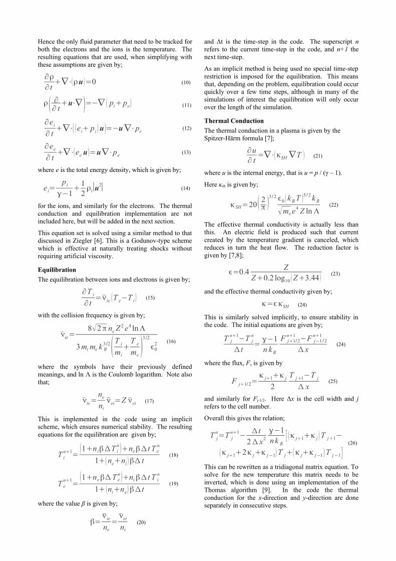
Extensive tests of problems relevant to fast-ignition have not yet been performed, however some tests of the code have been done. In figure 1 the initial density, ion temperature and electron temperature are shown respectively, alongside the values at 20 ps. In this problem a 10 μm region of an aluminium plasma has an electron temperature profile given by;

T eV=400 e−

x2

2σ2

+100

where σ = 25 μm. The rest of the plasma has an initial temperature of 100 eV. In the central 10 μm region the density is 2700 kg m-3, solid density for aluminium. The remainder is at one thousandth of aluminium solid density.

It can be seen that after 20 ps the temperature of the ions and electrons are identical. The initial higher density plasma has remained largely intact.

Conclusions

A discussion has been given of the creation of a 2D hydrodynamics code, which includes treatment of an ion and electron species with different temperatures. Ion-electron equilibration has been implemented along with thermal conductivity and the results of a simulation has been shown.

Future work needs to be done in using this code to look at problems relevant to fast-ignition. This will be done by taking temperature profiles from other simulations and looking at the hydrodynamic response of the plasma to the return current heating the target is subjected to.

References

1. Nuckolls J et al. 1972 Nature 239 139

2. Lindl J 1995 Phys. Plasmas 2 3933

3. Stephnes R et al. 2004 Phys. Rev E. 69 066414

4. Robinson A P L et al. 2007 Phys. Plasmas 14 083105

5. Kar S et al. 2009 Phys. Rev. Lett. 102 055001

6. Ziegler U 2004 J. Comp. Phys. 196 393

7. Spitzer L 1962 Physics of Fully Ionized Gases

8. Schurtz G et al. 2000 Phys. Plasmas 7 10

9. Press W H et al. 1986 Numerical Recipes in Fortran 90, Second Edition

Initial 20 ps

Figure 1: Spatial profiles for density (top), ion temperature (middle) and electron temperature (bottom) at 0 ps and 20 ps. It can be seen the electrons and ions have reached equilibrium after 20 ps. This is for an aluminium plasma initially at rest.

Evolution of a short pulse via ray tracing

Contact: rac@st-andrews.ac.uk

R.A. CairnsUniversity of St AndrewsSchool of Mathematics and StatisticsSt Andrews, Fife, KY16 9SS

1 Introduction

In a recent paper [1] we have suggested a way in which theradiation pattern produced by an antenna can be repro-duced in detail by following rays. The method relies onthe use of the asymptotic method of stationary phase tond the wave amplitude and phase in the far eld regionaway from the antenna, the innovative feature being thedevelopment of a method that does not depend on havingexplicit knowledge of the phase or a solution in terms of aphase integral. The required information is obtainable bylooking at di¤erences between adjacent rays. Examplesfor which an explicit solution can be found and comparedwith the approximation show that it works well exceptin the vicinity of a region where rays are reected. Ourobject here is to adapt this method to study the evolutionof short pulses launched into a time and space dependentmedium, a problem with possible relevance to some laserplasma systems.

2 Theory

We consider a one-dimensional problem with a short pulselaunched from x = 0 into the region x > 0. The time de-pendence of the pulse will be assumed centered aroundt = 0 and we shall assume that the pulse is propagatinginto a cold plasma so that the local dispersion relation is

D = !2 !2p k2c2 = 0 (1)

with !p; the plasma frequency, a function of x and t:With a time-dependent plasma frequency the wave fre-quency changes as it propagates, as can be seen from thestandard ray-tracing equations [2] and applications of thisphoton acceleration to laser plasma have been explored byMendonça [3]. The initial pulse launched from x = 0 canstill be Fourier transformed in time, even though the fre-quencies change as the wave propagates and, since we aredealing with a linear problem, the wave eld is a super-position of these initial Fourier components. The rate ofchange of the background plasma is assumed such thatthere is no appreciable change during the time taken tolaunch the pulse. We shall use as the Fourier trans-form variable of the initial pulse and ! for the frequencyfollowing a ray.In principle the wave amplitude at any point will

be a summation over the di¤erent Fourier compo-nents. We shall assume that the solution at any point

for a given Fourier component can be expressed as aslowly varying amplitude and a phase, taking the formA(; x; t) exp [i (; x; t)] : The full solution will then takethe form

a(x; t) =

Z 1

1A(; x; t) exp [i (; x; t)] d: (2)

The essence of the method of stationary phase [4] is toassume that rapid variations in the phase factor cancelout over most of the range of integration and that thedominant contribution comes from the neighbourhood ofpoints where

@

@[ (; x; t)] = 0: (3)

Taking this to be the case and letting 0 be the frequencyat which (3) is satised, we then approximate the integralbyZ 1

1A(0; x; t) exp

i (0; x; t) + i

1

2( 0)2 00(0; x; t)

d

= A(0; x; t)

s2

j00jeii4 (4)

where the sign in the exponential correponds to that of00 and the primes denote derivatives with repect to :The problem we now address is how to obtain the sec-ond derivative of the phase in the absence of any explicitexpression for :We begin by relating the problem to ray tracing. The

standard ray racing equations [2] are

x =

@D@k@D@!

k =

@D@x@D@!

(5)

! =

@D@t@D@!

where D is dened by (1) and its dependence on x andt is through that of the plasma frequency. Since thewavenumber and frequency are related to the phase by

k =@

@x(6)

! = @@t

the phase along a ray path is

=

Z(kdx !dt) ;

with the integral starting at the origin, and

@

@=

Z @k

@dx @!

@dt

=

Z @k@

@D@k +

@!@

@D@!

@D@!

dt

using (5). The numerator in this integral is the totalderivative of D with respect to and is zero since D isidentically zero. We conclude then that d

d is zero alonga ray path and so the point of stationary phase at anyvalue of x and t is determined by the initial frequencysuch that a ray launched from the origin at t = 0 arrivesat that point. That being so we now need to calculate thesecond derivative of the phase in order to nd the waveamplitude from (4).Following the method of [1] we note that following the

ray path

@2

@2=

Z @2k

@2dx @2!

@2dt

= Z

@2k@2

@D@k +

@2!@2

@D@!

@D@!

dt

and that by using the fact that the total derivative of Dis zero we can obtain an expression involving rst deriv-atives of the wavenumber and frequency with respect tothe launch frequency. Since these derivatives need to beevaluated numerically, this should allow better accuracythan using the original expression with second derivatves.The integral is taken from t = 0; x = 0 along the raytrajectory. Note that all rays are launched at the sametime, the time dependence of the pulse being implicit inits Fourier spectrum rather than in the launch conditions.This is analogous to the spatial problem where the raysare all launched from the centre of the antenna. In thelatter case the solution is only valid su¢ ciently far fromthe antenna (a few antenna widths in practice) and in thepresent case the solution is only valid su¢ ciently far fromthe origin that the solution is dominated by the dispersionof the di¤erent frequency components.At this point it will be useful to illustrate the method

with a simple example, namely a short pulse launched intoa homogeneous plasma. The solution of this problem canbe found exactly and is

a(x; t) =

Z 1

1

~a () exp

i2 !2p

x it

d (7)

with~a the Fourier transform of the time-dependence of

the pulse launched from x = 0. This illustrates the wayin which the solution is a superposition of the di¤erent

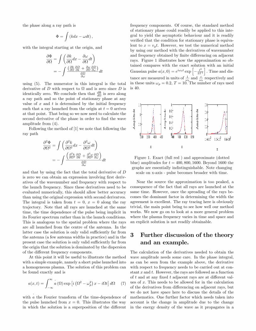
frequency components. Of course, the standard methodof stationary phase could readily be applied to this inte-gral to yield the asymptotic behaviour and it is readilyveried that the condition for stationary phase is equiva-lent to x = vgt. However, we test the numerical methodby using our method with the derivatives of wavenumberand frequency obtained by nite di¤erencing on adjacentrays. Figure 1 illustrates how the approximation so ob-tained compares with the exact solution with an initial

Gaussian pulse a(x; 0) = ei!0t exph t2

2T 2

i: Time and dis-

tance are measured in units of 1!0and c

!0respectively and

in these units !p = 0:2, T = 10: The number of rays usedis 40.

Figure 1. Exact (full red ) and approximate (dottedblue) amplitudes for t = 400; 800; 1600: Beyond 1600 thegraphs are essentially indistinguishable. Note changingscale on x-axis - pulse becomes broader with time.

Near the source the approximation is too peaked, aconsequence of the fact that all rays are launched at thesame time. However, once the spreading of the rays be-comes the dominant factor in determining the width theagreement is excellent. The ray tracing here is obviouslytrivial, the main point being to see how well our methodworks. We now go on to look at a more general problemwhere the plasma frequency varies in time and space andan explicit solution is not readily obtainable.

3 Further discussion of the theoryand an example.

The calculation of the derivatives needed to obtain thewave amplitude needs some care. In the phase integral,as can be seen from the example above, the derivativewith respect to frequency needs to be carried out at con-stant x and t. However, the rays are followed as a functionof t and at any xed t adjacent rays are at di¤erent val-ues of x: This needs to be allowed for in the calculationof the derivatives from di¤erencing on adjacent rays, butwe do not have space here to discuss the details of themathematics. One further factor which needs taken intoaccount is the change in amplitude due to the changein the energy density of the wave as it propagates in a

changing medium. This is separate from the e¤ect of dis-persion of the waves which we have considered so far. Ifwe express the amplitude in terms of the vector poten-tial a of the wave, then as shown by [5] the quantity !a2

is conserved for each frequency component, assuming thegradients in space or time to be small. This means that,in our one-dimensional problem,

@

@t

!a2

+@

@x

vg!a

2= 0: (8)

Following a ray path this implies that

d

dt

!a2

=@

@t

!a2

+ vg

@

@x

!a2

=

!a2

@vg@x: (9)

Now@vg@x

= 1q!2 !2p

!p!

@!p@x

while from the ray tracing equations

k = !p

!

@!p@x

so that (9) becomes

!a2

1 ddt

!a2

+ k1

dk

dt= 0 (10)

implying that k!a2 is constant along the ray. The am-plitude variation implied by this is included as an e¤ectadditional to that due to the spreading of the rays.To illustrate the method we look at a pulse (as before)

being overtaken by a moving density ramp as illustratedin Figure 2. The peak of the pulse has been reduced to0:25 in the gure for convenience. We use 100 rays, ini-tially spread across the spectrum of the pulse. Since itstime prole is Gaussian, so too is the spectrum, and therays initially are spaced evenly over 2:5 standard devi-ations from the centre, at 1 in our normalised units.

Figure 2. Initial pulse shape (blue) and density prole(red) in terms of critical density for frequency !0:The

prole moves to the right with velocity 0:98c:

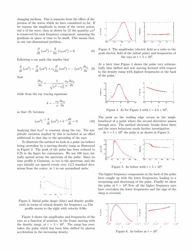
Figure 3 shows the amplitudes and frequencies of therays as a function of position, in the frame moving withthe density ramp, at t = 5 103. The ramp has over-taken the pulse which has been blue shifted by photonacceleration in the increasing density.

Figure 3. The amplitudes (electric eld as a ratio to thepeak electric eld of the initial pulse) and frequencies of

the rays at t = 5 103:

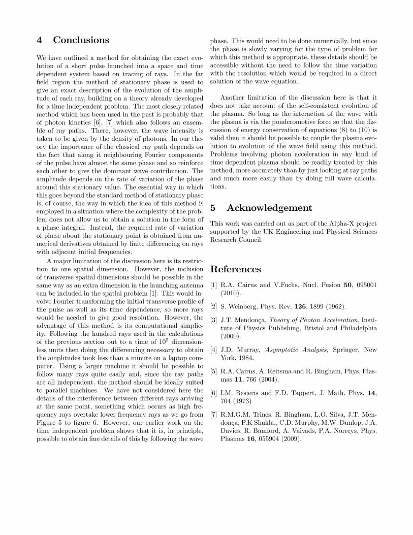
At a later time Figure 4 shows the pulse very substan-tially blue shifted and now moving forward with respectto the density ramp with highest frequencies at the backof the pulse.

Figure 4. As for Figure 3 with t = 2:5 104:

The peak on the trailing edge occurs in the neigh-bourhood of a point where the second derivative passesthrough zero. The method obviously breaks down thereand the exact behaviour needs further investigation.At t = 5 104 the pulse is as shown in Figure 5.

Figure 5. As before with t = 5 104:

The higher frequency components at the back of the pulsehave caught up with the lower frequencies, leading to asteepening and shortening of the pulse. Finally we showthe pulse at t = 105:Now all the higher frequency rayshave overtaken the lower frequencies and the sign of thechirp is reversed.

Figure 6. As before at t = 105:

4 Conclusions

We have outlined a method for obtaining the exact evo-lution of a short pulse launched into a space and timedependent system based on tracing of rays. In the fareld region the method of stationary phase is used togive an exact description of the evolution of the ampli-tude of each ray, building on a theory already developedfor a time-independent problem. The most closely relatedmethod which has been used in the past is probably thatof photon kinetics [6], [7] which also follows an ensem-ble of ray paths. There, however, the wave intensity istaken to be given by the density of photons. In our the-ory the importance of the classical ray path depends onthe fact that along it neighbouring Fourier componentsof the pulse have almost the same phase and so reinforceeach other to give the dominant wave contribution. Theamplitude depends on the rate of variation of the phasearound this stationary value. The essential way in whichthis goes beyond the standard method of stationary phaseis, of course, the way in which the idea of this method isemployed in a situation where the complexity of the prob-lem does not allow us to obtain a solution in the form ofa phase integral. Instead, the required rate of variationof phase about the stationary point is obtained from nu-merical derivatives obtained by nite di¤erencing on rayswith adjacent initial frequencies.A major limitation of the discussion here is its restric-

tion to one spatial dimension. However, the inclusionof transverse spatial dimensions should be possible in thesame way as an extra dimension in the launching antennacan be included in the spatial problem [1]. This would in-volve Fourier transforming the initial transverse prole ofthe pulse as well as its time dependence, so more rayswould be needed to give good resolution. However, theadvantage of this method is its computational simplic-ity. Following the hundred rays used in the calculationsof the previous section out to a time of 105 dimension-less units then doing the di¤erencing necessary to obtainthe amplitudes took less than a minute on a laptop com-puter. Using a larger machine it should be possible tofollow many rays quite easily and, since the ray pathsare all independent, the method should be ideally suitedto parallel machines. We have not considered here thedetails of the interference between di¤erent rays arrivingat the same point, something which occurs as high fre-quency rays overtake lower frequency rays as we go fromFigure 5 to gure 6. However, our earlier work on thetime independent problem shows that it is, in principle,possible to obtain ne details of this by following the wave

phase. This would need to be done numerically, but sincethe phase is slowly varying for the type of problem forwhich this method is appropriate, these details should beaccessible without the need to follow the time variationwith the resolution which would be required in a directsolution of the wave equation.

Another limitation of the discussion here is that itdoes not take account of the self-consistent evolution ofthe plasma. So long as the interaction of the wave withthe plasma is via the ponderomotive force so that the dis-cussion of energy conservation of equations (8) to (10) isvalid then it should be possible to couple the plasma evo-lution to evolution of the wave eld using this method.Problems involving photon acceleration in any kind oftime dependent plasma should be readily treated by thismethod, more accurately than by just looking at ray pathsand much more easily than by doing full wave calcula-tions.

5 Acknowledgement

This work was carried out as part of the Alpha-X projectsupported by the UK Engineering and Physical SciencesResearch Council.

References

[1] R.A. Cairns and V.Fuchs, Nucl. Fusion 50, 095001(2010).

[2] S. Weinberg, Phys. Rev. 126, 1899 (1962).

[3] J.T. Mendonça, Theory of Photon Acceleration, Insti-tute of Physics Publishing, Bristol and Philadelphia(2000).

[4] J.D. Murray, Asymptotic Analysis, Springer, NewYork, 1984.

[5] R.A. Cairns, A. Reitsma and R. Bingham, Phys. Plas-mas 11, 766 (2004).

[6] I.M. Besieris and F.D. Tappert, J. Math. Phys. 14,704 (1973)

[7] R.M.G.M. Trines, R. Bingham, L.O. Silva, J.T. Men-donça, P.K Shukla., C.D. Murphy, M.W. Dunlop, J.A.Davies, R. Bamford, A. Vaivads, P.A. Norreys, Phys.Plasmas 16, 055904 (2009).

1

Calculation of Siegert states of molecules in electric field :an H+

2 study

contact : linda@power1.pc.uec.ac.jp, lhamonou01@qub.ac.uk

Linda Hamonou

University of Electro-communications,1-5-1, Chofu-ga-oka, Chofu-shi, Tokyo, Japan.

Toru Morishita

University of Electro-communications,1-5-1, Chofu-ga-oka, Chofu-shi, Tokyo, Japan.

Oleg I. Tolstikhin

Russian Research Center ”Kurchatov Insti-tute”Kurchatov Square 1, Moscow 123182, Russia

Shinichi Watanabe

University of Electro-communications,1-5-1, Chofu-ga-oka, Chofu-shi, Tokyo, Japan

1. Introduction

Siegert states of atoms and molecules

placed in an electric field, defined as the so-

lutions to the stationary Schrodinger equa-

tion satisfying the regularity and outgoing-

wave boundary conditions [2], have been

obtained by Batishchev et al [1] within

th restriction of the single active electron

(SAE) approximation. In [1] was presented

an efficient method to calculate not only

the complex energy eigenvalues, but also

the eigenfunctions for a general class of

one-electron atomic potentials. They also

derived an exact expression for the trans-

verse momentum distribution of the ionized

electrons in terms of Siegert eigenfunction

in the asymptotic region.

In the previous CLF report we pre-

sented an extension of the Siegert states

to molecules. The formulation of computa-

tional method requires some modifications

from the atomic procedure.

In this report we present the prelimi-

nary results obtained using the molecular

formulation to study the simplest molecu-

lar ion, H+2 . We first give the basic equa-

tion required for understanding the Siegert

states of molecules. Then we explain the

numerical procedure including a DRV ba-

sis set and R-matrix propagation. Results

have been obtained for different potential

models of H+2 for an internuclear distance

of R=2 and an angle between the electric

field direction and the molecular axis θ = 0.

We use atomic units through the report in

not specified otherwise.

2. Basic equations

The Siegert states of molecules are ob-

tained within the SAE approximation by

solving the following Schrodinger equation

Hϕ = Eϕ (1)

The Hamiltonian for an electron interact-

ing with a molecular potential V (r) in pres-

ence of a static uniform electric field F di-

rected along the z axis is given by :

H = −1

2∆ + V (r) + Fz. (2)

We use the parabolic coordinates η, ϕ

2

and ξ defined as follow.

ξ = r + z, 0 ≤ ξ ≤ ∞ (3)

η = r − z, 0 ≤ η ≤ ∞ (4)

ϕ = arctany

x, 0 ≤ ϕ ≤ 2π(5)

In the general cases, for an arbitrary molec-

ular potential V (r), the variables (ξ, η) and

φ cannot be separated as they are for the

atomic case. In order to solve the molec-

ular problem we have to take into account

a coupling in ϕ. The Schrodinger equation

(1) in paraboliccoordinates is rewritten in

the form

[∂

∂ηη∂

∂η− 1

4η

∂2

∂ϕ2+ B(η) +

Eη

2+Fη2

4

]ψ(ξ, η, ϕ) = 0, (6)

where

B(η) =∂

∂ξξ∂

∂ξ− 1

4ξ

∂2

∂ϕ2− ξ + η

2V (ξ, η) +

Eξ

2− Fξ2

4. (7)

These equations must be supple-

mented by the regularity and out-going-

wave boundary conditions [2]. For non-

zero electric fields, all the eigenstates are

unbound, so the eigenvalue E is a complex

number

E = E − i

2Γ (8)

with the real part E giving the energy of

the state, and the imaginary part Γ defin-

ing the ionisation rates. Equation () and

(7) are solved using the slow-variable dis-

cretization (SVD) method [3] in combina-

tion with the R-matrix propagation tech-

nique [4].

3. Numerical procedure

The numerical procedure is based on the

discrete variable representation (DVR) ba-

sis sets [5] constructed from Laguerre, Ja-

cobi and Legender polynomials compatible

with the boundary conditions [6]. We re-

fer the reader to [1] for more mathematical

and numerical details.

In the atomic case [1], the eigenfunc-

tions of the adiabatic Hamiltonian were

obtained using the DVR constructed us-

ing the generalized Laguerre polynomials

L|m|n (sξ) [6], where the scaling s defines the

extent of the DVR basis in ξ.

This representation enables the exact in-

corporation of the regularity boundary con-

dition ψ(ξ, η)|ξ→0 ∝ ξ|m|/2 into the formu-

lation. In the molecular case, the solution

ψ(ξ, η, ϕ) contains integer and half-integer

powers of ξ for ξ → 0 which cannot be rep-

resented by a single Laguerre-DVR basis

with a fixed magnetic quantum number m.

We thus introduce a new variable.

ξ = ζ2 (9)

So we have

B(η) =B(η)

4ζ(10)

with

B(η) =∂

∂ζζ∂

∂ζ+

(1

ζ+ζ

η

)∂2

∂ϕ2− 2ζ(ζ2 + η)V (ξ, η, ϕ) + 2Eζ3 − Fζ5. (11)

3

This transformation allows us to use a

single-Laguerre-DVR basis with m = 0 for

the expansion in ζ. The eigenfunctions of

B(η) are constructed using the direct prod-

uct of the Laguerre-DVR basis with peri-

odic boundary conditions in ϕ.

In the R-matrix theory [7], the space

is divided into two regions, an inner region

which is here divided into Nsec sectors so

that 0 ≤ η ≤ ηc can be define by

0 = η0 < η1 < · · · < ηNsec = ηc. (12)

In each sector, we construct the R-matrix

basis ψn(ξ, η, ϕ) defined by[∂

∂ηη∂

∂η− L− 1

4η

∂2

∂ϕ2+ B(η) +

Eη

2+Fη2

4

]ψ(ξ, η, ϕ) = 0, (13)

with L is the Bloch operator given by:

L = η[δ(η − η+)− δ(η − η−)]∂

∂η. (14)

Similarly to the η variable, in the molecu-

lar problem in order to incorporate the reg-

ularity boundary condition ψ(ξ, η)|η→0 ∝η|m|/2, the solution contains integer and

half-integer powers of η. We thus introduce

another change of variables in the first sec-

tor,

η = χ2 (15)

to allow the representation of the solution

by a single Legendre-DVR basis. In the

outer region, η > ηc, the molecular po-

tential is substituted by a purely Coulomb

potential −Zas/r so that the problem be-

comes exactly separable in parabolic coor-

dinates and reduced to solving uncoupled

equations in η [1]. We apply out-going

wave boundary condition. The R-matrix is

propagated from η = 0 outward and from

η = ηc inward. Matching the solutions

at the right boundary in the first sector

gives the Siegert eigenvalue E and eigen-

functions.

4. Results

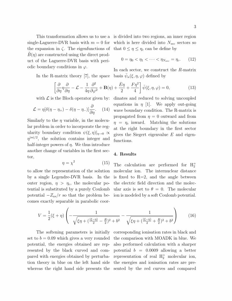
The calculation are performed for H+2

molecular ion. The internuclear distance

is fixed to R=2, and the angle between

the electric field direction and the molec-

ular axis is set to θ = 0. The molecular

ion is modeled by a soft Coulomb potential.

V =1

2(ξ + η)

− 1√ξη + ( (ξ−η)

2− R

2)2 + b2

− 1√ξη + ( (ξ−η)

2+ R

2)2 + b2

(16)

The softening parameters is initially

set to b = 0.09 which gives a very rounded

potential, the energies obtained are rep-

resented by the black curved and com-

pared with energies obtained by perturba-

tion theory in blue on the left hand side

whereas the right hand side presents the

corresponding ionisation rates in black and

the comparison with MOADK in blue. We

also performed calculation with a sharper

potential b = 0.0009 allowing a better

representation of real H+2 molecular ion,

the energies and ionisation rates are pre-

sented by the red curves and compared

4

as well with perturbation theory’s energies

and MOADK [10] ionisation rates in green.

We obtain a good agreement with pertur-

bation theory for electric field F < 0.25

which is to be expected as perturbation

theory is limited to low electric field. We

can also notice that for the rounded po-

tential with b = 0.09 our ionisation rates

are lower than the one given by MOADK

which is also to be expected as MOADK

tend to overestimate the ionisation rates.

However the ionisation rate obtained for

the sharper potential with b = 0.0009 is

much higher than the value obtained with

MOADK. For sharper potential, as bound-

ing energy increases, the ioinsation rates

decreases leading to an underestimation of

the ionisation rates by MOADK.

0 0.1 0.2 0.3 0.4 0.5Electric field F (a.u.)

-1.6

-1.5

-1.4

-1.3

-1.2

-1.1

-1

-0.9

Ene

rgy

(a.u

.)

b=0.09b=0.0009perturbation theory b=0.09perturbation theory b=0.0009

0 0.1 0.2 0.3 0.4 0.5Electric field F (a.u.)

1e-12

1e-10

1e-08

1e-06

0.0001

0.01

1

Ioni

satio

n ra

tes

(a.u

.)

b=0.09b=0.0009MOADK b=0.09MOADK b=0.0009

Figure 1. Electric field dependent energies and ionisation rates obtained with twodifferent potential and compared with other theory.

5. Conclusion

In this report, we have presented the devel-

opment necessary to calculate the molecu-

lar Siegert states in a static electric field.

Starting from an atomic problem enabling

the calculation of Siegert states in the sin-

gle active electron approximation, we ex-

tended the problem reducing the use of the

symmetries and including the coupling in

ϕ coordinate to solve molecular problems.

This new method enable us to obtain eigen-

values and eigenfunctions for a particular

Siegert state as a function of a variating

electric field for molecules modeled by one-

electron potential. The complex eigenvalue

obtained from the match of the R-matrix

with the out-going wave Siegert boundary

condition gives the energy and the ioniza-

tion rate of a particular state.

5

6. Reference

1. P. A. Batishchev, O. I. Tolstikhin and

T. Morishita, Phys. Rev. A 82, 023416

(2010)

2. A. J. F. Siegert, Phys. Rev. 56, 750

(1939)

3. O. I. Tolstikhin, S. Watanabe and M.

Matsuzawa, J. Phys. B 29, L389 (1996)

4. K. L. Baluja, P. G. Burke and L. A.

Morgan, Comput. Phys. Commun. 27,

299 (1982)

5. D. O. Harris, G. G. Engerholm and W.

D. Gwinn, J. Chem. Phys. 43, 1515 (1965)

6. A. S. Dickinson and P. R. Certain, J.

Chem. Phys. 49, 4209 (1968)

7. J. C. Light, I. P. Hamilton and J. V.

Lill, J. Chem. Phys. 82, 1400 (1985)

8. O. I. Tolstikhin and C. Namba, CTBC

- A Program to Solve the Collinear three-

Body Problem: Bound States and Scat-

tering Below the Three-body Disintegra-

tion Threshold, Research Report NIFS-

779 (National Institute for Fusion Sci-

ence, Toki, Japan, 2003). Available at

http://www.nifs.ac.jp/report/nifs779.html

9. P.G. Burke and K. A. Berrington,

Atomic and Molecular Processes: An R-

matrix Approach (IOP, Bristol, 1993)

10. X. M. Tong, Z. X. Zhao and C. D. Lin,

Phys. Rev. A 66, 033402 (2002)

Radiation Reaction in Ultra-Intense Laser Fields

Tom Heinzl

School of Computing and Mathematics, University of Plymouth,

Plymouth PL4 8AA, UK

Chris Harvey

Department of Physics, Umeå University,

SE-901 87 Umeå, Sweden

Introduction

The problem of classical radiation reaction (RR) has vexed

generations of physicists since its first formulation in 1892 by

Lorentz [1, 2]. Following important contributions by Abraham

[3] and others the equation describing the back reaction of the

radiation field on the motion of the radiating charge has been

cast in its final covariant form by Dirac in 1938 [4]. It is now

aptly called the Lorentz-Abraham-Dirac (LAD) equation. The

relevant body of literature has become enormous and we refer

to the recent monographs [5, 6] and, in particular, to the preprint

[7] for an overview of the historical development and extensive

lists of references. A particularly compact way of writing the

LAD equation, say for an electron (mass m, charge e) is

where u denotes the electron 4-velocity, F = eFu/c the Lorentz

4-force in terms of the field strength tensor, F, of the externally

prescribed field and dots derivatives with respect to proper

time, τ. The second term on the right is the RR force, FRR,

which is characterised by the appearance of the time parameter

This is the time it takes light to traverse the classical electron

radius1, re = e2/4πmc2 = αλC ≈ 3 fm. Obviously, the scales

involved are typical for strong interactions (or quantum

chromodynamics) – a first hint that the classical LAD equation

(1) does not capture the physics at these (essentially quantum)

scales. Finally, the projection Pµν = 1 – uµuν /c2 in (1) guarantees

that 4-acceleration and velocity are Minkowski orthogonal. This

follows upon differentiating the on-shell condition, u2= c2,

which, of course, is Einstein's first postulate on the universality

of the speed of light, c. As u is time-like, its τ-derivative is

space-like.

Estimating RR

The LAD equation (1) is of third order in time derivatives and

hence suffers from a number of pathologies such as runaway

solutions and pre-acceleration. One way to overcome this is by

iteration, assuming that FRR << F which amounts to working to

first order in τ0. This in turn implies a ‘reduction of order’ in

derivatives and results in the Landau-Lifshitz (LL) equation [8],

Hence, one replaces the problematic ‘jerk’ [9] term, mü, in (1)

by the proper time derivative of the Lorentz force [6] where the

acceleration term is evaluated to lowest order in τ0, hence

1 We employ Heaviside-Lorentz units with fine structure constant α =

e2/4πħc = 1/137.

For alternative derivations of the LL equation emphasising

mathematical intricacies related to regularisations of the point

particle concept we refer to [10, 11].

The LL equation (3) was derived under the assumption of a

small reaction force, FRR << F. Let us elucidate the physics

involved somewhat further by assuming that the external field is

produced by a laser modelled as a plane wave with light-like

wave vector k, k2 = 0. An electron ‘approaching’ the laser field

with initial 4-velocity u0 will, in its rest frame, ‘see’ a wave

frequency given by the invariant scalar product,

Temporal gradients will then be of the order of the laser period,

dF/dτ ~ Ω0F, so that the relative magnitude of the reaction force

becomes

with the inequality required for the validity of the LL equation.

Consider now a head-on collision in the lab where the laser

frequency is measured to be ω,

with the usual relativistic gamma factor, γ0 = Ee/mc2 measuring

the electron energy Ee in units of mc2. Such an electron then

‘sees’ a laser frequency that is Doppler upshifted according to

the last identity holding for γ0 >>1.This boost in laser frequency

is just the usual energy gain of a colliding versus fixed target

mode (which, of course, are related by a longitudinal Lorentz

boost with rapidity ζ). If we define dimensionless photon

energies in the co-moving and lab frames,

the RR parameter r from (6) becomes

For an optical laser ν ≈ 10-6 so that r ≈ 10-8 γ0.Thus, to boost

this to order unity (such that reaction equals Lorentz force)

requires γ0 ≈ 108 i.e. electron energies of order ≈ 102 TeV.

These can only be produced in gamma-ray bursts, but not

(currently) in labs. The ground breaking laser pair production

(“matter from light”) experiment SLAC E-144, for instance,

was utilising the 50 GeV SLAC linear collider implying γ0 ≈ 105

and r ≈ 10-8 [12].

The standard way of quantifying radiation by accelerated

charges is via Larmor's formula for the radiated power, the

relativistic incarnation of which may be written as

and hence is of order τ0. If we follow our philosophy of

neglecting terms of order τ02 it suffices to express the

acceleration via just the Lorentz force,

where we have introduced the 4-vector E corresponding to the

electric field ‘seen’ by the electron. Let us reemphasise here

that we do not require the LL equation with its RR force, FRR.

Thus, if we assume transversality of our laser fields, kF = 0, we

Contact theinzl@plymouth.ac.uk

immediately derive a very useful conservation law by dotting k

into (12),

Hence, without RR, the electron always ‘sees’ the same laser

frequency on its passage through the laser beam,

If we now plug the Lorentz equation (12) into (11) the average

energy loss per (reduced) laser period 1/ Ω0 in units of mc2

becomes

Interestingly, we recover our RR parameter r from (6) and (10)

plus a new quantity, the dimensionless laser amplitude a0 which

measures the energy gain of an electron traversing a laser

wavelength, c/Ω0, in an rms field E in units of mc2. Obviously,

when this (purely classical) parameter becomes of order unity,

the electron motion is relativistic. Note that a0 is both Lorentz

and gauge invariant [13]. This is particularly obvious upon

reexpressing a0 in terms of a dimensionless field strength,

whereupon

The energy loss parameter (15) was previously employed in

[14—17]. It suggests that for substantial radiation the small RR

parameter r needs to be compensated by large values of a02.

Denoting the current record intensity by I22 = 1022 W/cm2 we

may write

so that one can envisage a0 values of about 103 for the not too

distant future [18,19]. We have seen already in (10) that large

gamma factors (colliding mode) yield a further increase of

radiative losses. In addition, the losses accumulate over

successive laser periods. After, say, N cycles one expects a total

relative change of the electron gamma factor given by

where the smallness of αν ≈ 10-8 may be compensated by pulse

duration, N, initial electron energy, γ0, and intensity, a02.

Modelling the laser

The simplest model of a laser (beam) is provided by a plane

wave with a field tensor depending solely on the invariant

phase, F = F(φ), φ = k · x, and obeying transversality, kF = 0. If

we choose k as in (7) we have

In other words, the laser field F only depends on the light-front

or null coordinate, x– = ct – z.

Plane waves are invariantly characterised as null fields [21, 22]

as scalar and pseudoscalar invariants vanish,

Hence, the energy momentum tensor of a plane wave is just F2.

This is the only nontrivial power of field strength as F is

nilpotent with index 3, i.e. F3 = 0 which will be important when

we solve the equations of motion in such a field. As a result it is

important to note that there is no intrinsic invariant scale

associated with a null field. In order to characterise them in an

invariant fashion one needs a probe such as an electron or a

(non-laser) photon. This naturally leads to the invariant

amplitude a0 as defined in (16) which explicitly depends on the

probe electron 4-velocity. Defining the energy density of the

laser ‘seen’ by the electron as

we see that (16) expresses just the dimensionless version of this

energy density,

Typically, the plane wave modelling the laser will be pulsed,

i.e. of finite duration in invariant phase, φ. We accommodate

this situation by parameterising F as follows. We assume the

plane wave field to be linearly polarised along the space-like

transverse 4-vector ε (ε2 = –1) and hence decompose F into

magnitude a0, envelope f = f(φ) and a constant tensor,

,

so that we have altogether

with the dimensionless constant 4-vector n = kc/Ω0 obeying n2 =

0 = n · ε and n · u = n · u0 = c. As a result,

,

with all higher powers vanishing due to n2 = 0. In order for (26)

to be consistent with (16) and (25) the average must be defined

in such a way that f is normalized to unity. Defining a

dimensionless gauge potential, Â = eA/mc2, the field strength

becomes

the prime henceforth denoting the derivative with respect to

invariant phase φ. Comparison with (26) finally yields Â′= a0 f ε

and

Solving the LL equation

Unlike the LAD the LL equation is a fairly standard equation of

motion being second order in time derivatives. Hence, it

requires two integrations and initial conditions for velocity and

position. For the purposes of this contribution it will be

sufficient to perform only the first integration for which we

need to provide the initial 4-velocity, u(0) = u0.

Neglecting RR

To set the stage for a later comparison we first briefly recall the

solution without RR, i.e. of the Lorentz force equation of

motion (12). We first note that for any function f = f(τ) of

proper time we may trade derivatives according to

where, in the last step, we have used the conservation law (14).

In terms of the dimensionless field strength (27) the Lorentz

equation takes on the particularly compact form

This is, of course, integrated by a matrix exponential which

truncates at second order due to nilpotency, F3 = 0. Employing

the parameterisation (26) the solution becomes

where we have used the pulse shape integral

for k = 1. Upon inspection of the solution (30) we note the

following features. The velocity decomposes into transverse

and longitudinal contributions given by the second and third

terms on the right, respectively. If the initial velocity is

longitudinal (like for a head-on collision) we have ε ·u0=0. In

this case, the longitudinal velocity is quadratic in a0 while the

transverse component is always linear.

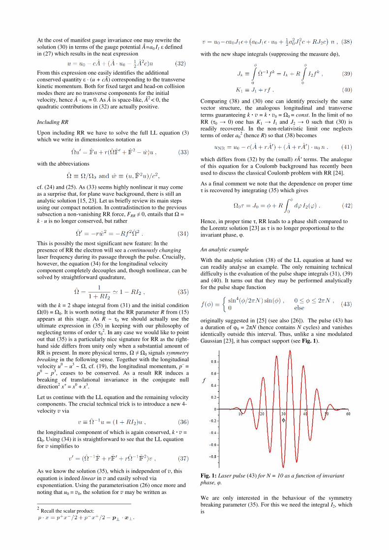
At the cost of manifest gauge invariance one may rewrite the

solution (30) in terms of the gauge potential Â=a0 I1 ε defined

in (27) which results in the neat expression

From this expression one easily identifies the additional

conserved quantity ε · (u + cÂ) corresponding to the transverse

kinetic momentum. Both for fixed target and head-on collision

modes there are no transverse components for the initial

velocity, hence  · u0 = 0. As  is space-like, Â2 < 0, the

quadratic contributions in (32) are actually positive.

Including RR

Upon including RR we have to solve the full LL equation (3)

which we write in dimensionless notation as

with the abbreviations

cf. (24) and (25). As (33) seems highly nonlinear it may come

as a surprise that, for plane wave background, there is still an

analytic solution [15, 23]. Let us briefly review its main steps

using our compact notation. In contradistinction to the previous

subsection a non-vanishing RR force, FRR ≠ 0, entails that Ω =

k · u is no longer conserved, but rather

This is possibly the most significant new feature: In the

presence of RR the electron will see a continuously changing

laser frequency during its passage through the pulse. Crucially,

however, the equation (34) for the longitudinal velocity

component completely decouples and, though nonlinear, can be

solved by straightforward quadrature,

with the k = 2 shape integral from (31) and the initial condition

Ω(0) = Ω0. It is worth noting that the RR parameter R from (15)

appears at this stage. As R ~ τ0 we should actually use the

ultimate expression in (35) in keeping with our philosophy of

neglecting terms of order τ02. In any case we would like to point

out that (35) is a particularly nice signature for RR as the right-

hand side differs from unity only when a substantial amount of

RR is present. In more physical terms, Ω ≠ Ω0 signals symmetry

breaking in the following sense. Together with the longitudinal

velocity u0 – u3 ~ Ω, cf. (19), the longitudinal momentum, p– =

p0 – p3, ceases to be conserved. As a result RR induces a

breaking of translational invariance in the conjugate null

direction2 x+ = x0 + x3.

Let us continue with the LL equation and the remaining velocity

components. The crucial technical trick is to introduce a new 4-

velocity v via

the longitudinal component of which is again conserved, k · v =

Ω0. Using (34) it is straightforward to see that the LL equation

for v simplifies to

As we know the solution (35), which is independent of v, this

equation is indeed linear in v and easily solved via

exponentiation. Using the parameterisation (26) once more and

noting that u0 = v0, the solution for v may be written as

2 Recall the scalar product:

with the new shape integrals (suppressing the measure dφ),

Comparing (38) and (30) one can identify precisely the same

vector structure, the analogous longitudinal and transverse

terms guaranteeing k · v = k · v0 = Ω0 = const. In the limit of no

RR (τ0 → 0) one has K1 → I1 and J2 → 0 such that (30) is

readily recovered. In the non-relativistic limit one neglects

terms of order a02 (hence R) so that (38) becomes

which differs from (32) by the (small) rÂ′ terms. The analogue

of this equation for a Coulomb background has recently been

used to discuss the classical Coulomb problem with RR [24].

As a final comment we note that the dependence on proper time

τ is recovered by integrating (35) which gives

Hence, in proper time τ, RR leads to a phase shift compared to

the Lorentz solution [23] as τ is no longer proportional to the

invariant phase, φ.

An analytic example

With the analytic solution (38) of the LL equation at hand we

can readily analyse an example. The only remaining technical

difficulty is the evaluation of the pulse shape integrals (31), (39)

and (40). It turns out that they may be performed analytically

for the pulse shape function

originally suggested in [25] (see also [26]). The pulse (43) has

a duration of φ0 = 2πN (hence contains N cycles) and vanishes

identically outside this interval. Thus, unlike a sine modulated

Gaussian [23], it has compact support (see Fig. 1).

Fig. 1: Laser pulse (43) for N = 10 as a function of invariant

phase, φ.

We are only interested in the behaviour of the symmetry

breaking parameter (35). For this we need the integral I2, which

is

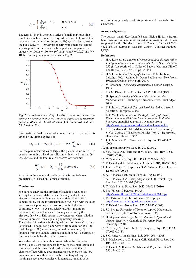
The term δI2 in (44) denotes a series of small amplitude sine

functions which we do not display. All we need to know is that

they vanish at the ‘end’ of the pulse, δI2(φ0) = 0. Hence, inside

the pulse Ω/Ω0 = 1 – RI2 drops linearly with small oscillations

superimposed until it reaches a final plateau. For parameter

values γ0 = 100, a0= 150, ν = 10-6 (implying R = 0.022) and N =

10 the resulting behaviour is shown in Fig. 2.

Fig. 2: Laser frequency Ω/Ω0 = 1 – RI2 as ‘seen’ by the electron

during the passing of an N =10 pulse as a function of invariant

phase, φ. Black line: Constant result (14) without RR. Red line:

RR Solution (35).

From (44) the final plateau value, once the pulse has passed, is

given by the simple expression

For the parameter values of Fig. 2 the plateau value is 0.81. In

general, assuming a head-on collision with γ0 >> 1 one has Ω0 ≈

2γ0, Ωf ≈ 2γf and the total relative energy loss becomes

Apart from the numerical coefficient this is precisely our

prediction (18) based on Larmor's formula.

Conclusions

We have re-analysed the problem of radiation reaction by

solving the Landau-Lifshitz equation analytically for an

electron in an intense plane wave laser field. Such a field

depends solely on the invariant phase, φ = k · x or, with the laser

wave vector k pointing in z direction, on the light-front

coordinate x– = ct – z. A particularly useful signature for

radiation reaction is the laser frequency as ‘seen’ by the

electron, Ω = k · u. This ceases to be conserved when radiation

reaction is present, thus signalling symmetry breaking:

Translational invariance in the light-front coordinate x+ = ct + z

is violated. For a pulsed plane wave of finite duration in x– the

total change in Ω (hence in longitudinal momentum, p–)

obtained from the Landau-Lifshitz equation is well described by

Larmor's formula for the radiated power.

We end our discussion with a caveat. While the discussion

above is consistent one expects, in view of the small length and

time scales and the huge field gradients involved, that all

classical effects will be accompanied (if not overwhelmed) by

quantum ones. Whether these can be disentangled, say by

looking at special observables or kinematics, remains to be

seen. A thorough analysis of this question will have to be given

elsewhere.

Acknowledgements

The authors thank Kurt Langfeld and Nicloa Iji for a fruitful

(and ongoing) collaboration on radiation reaction. C. H. was

supported by the Swedish Research Council Contract #2007-

4422 and the European Research Council Contract #204059-

QPQV.

References

1. H.A. Lorentz, La Théorié Electromagnétique de Maxwell et

son Application aux Corps Mouvants, Arch. Neérl. 25, 363-

552 (1892), reprinted in Collected Papers (Martinus Nijhoff,

The Hague, 1936), Vol. II, pp. 64-343.

2. H.A. Lorentz, The Theory of Electrons, B.G. Teubner,

Leipzig, 1906; reprinted by Dover Publications, New York,

1952 and Cosimo, New York, 2007.

3. M. Abraham, Theorie der Elektrizität, Teubner, Leipzig,

1905.

4. P.A.M. Dirac, Proc. Roy. Soc. A 167, 148-169 (1938).

5. H. Spohn, Dynamics of Charged Particles and their

Radiation Field, Cambridge University Press, Cambridge,

2004.

6. F. Rohrlich, Classical Charged Particles, 3rd ed., World

Scientific, Singapore, 2007.

7. K.T. McDonald, Limits on the Applicability of Classical

Electromagnetic Fields as Inferred from the Radiation

Reaction, unpublished preprint, available from:

http://www.hep.princeton.edu/~mcdonald/examples/

8. L.D. Landau and E.M. Lifshitz, The Classical Theory of

Fields (Course of Theoretical Physics, Vol. 2), Butterworth-

Heinemann, Oxford, 1987.

9. J.G. Russo and P.K. Townsend, J. Phys. A 42, 445402

(2009).

10. H. Spohn, Europhys. Lett. 49, 287 (2000).

11. S.E. Gralla, A.I. Harte and R.M. Wald, Phys. Rev. D 80,

024031 (2009).

12. C. Bamber et al., Phys. Rev. D 60, 092004 (1999).

13. T. Heinzl and A. Ilderton, Opt. Commun. 282, 1879 (2009).

14. J. Koga, T.Zh. Esirkepov and S.V. Bulanov, Phys. Plasmas

12, 093106 (2005).

15. A. Di Piazza, Lett. Math. Phys. 83, 305 (2008).

16. A. Di Piazza, K.Z. Hatsagortsyan and C.H. Keitel, Phys.

Rev. Lett. 102, 254802 (2009).

17. Y. Hadad et al., Phys. Rev. D 82, 096012 (2010).

18. The Vulcan 10 Petawatt Project:

http://www.clf.rl.ac.uk/New+Initiatives/14764.aspx

19. The Extreme Light Infrastructure (ELI) project:

http://www.extreme-light-infrastructure.eu

20. T. Heinzl, Lect. Notes Phys. 572, 55-142 (2001).

21. J.L. Synge, University of Toronto Applied Mathematics

Series, No. 1 (Univ. of Toronto Press, 1935).

22. H. Stephani, Relativity: An Introduction to Special and

General Relativity, Cambridge University Press,

Cambridge, 2004.

23. C. Harvey, T. Heinzl, N. Iji, K. Langfeld, Phys. Rev. D 83,

076013 (2011).

24. S.G. Rajeev, Annals Phys. 323, 2654-2661 (2008).

25. F. Mackenroth, A. Di Piazza, C.H. Keitel, Phys. Rev. Lett.

105, 063903 (2010).

26. T. Heinzl, A. Ilderton, M. Marklund, Phys. Lett. B 692,

250-256 (2010).

Time-dependent R-matrix theory for ultra-fast processes

S. Hutchinson Centre for Theoretical Atomic, Molecular and Optical Physics, Queen’s University Belfast, Belfast BT7 1NN, United Kingdom

A. C. Brown Centre for Theoretical Atomic, Molecular and Optical Physics, Queen’s University Belfast, Belfast BT7 1NN, United Kingdom

H.W. van der Hart Centre for Theoretical Atomic, Molecular and Optical Physics, Queen’s University Belfast, Belfast BT7 1NN, United Kingdom

Introduction Over the last ten years, substantial experimental effort has been devoted to the study of atomic and molecular processes on ultra-short timescales. At the heart of these developments lies harmonic generation, since ultra-short pulses are created through the superposition of several harmonics created by the same pulse [1]. Harmonic generation can also be used as a measurement tool, for example, to study molecular changes on the sub-femtosecond timescale [2], and to obtain information about molecular structure [3]. Harmonic generation has been used to explore the importance of ultra-fast multi-electron dynamics in molecules [4] and in atomic systems [5].

The most widely used approximation in theoretical work devoted to atoms in strong fields is the single-active-electron approximation. Within this approximation, only a single electron can respond to the laser field. This approximation is clearly invalid if we aim to investigate the influence of electron correlation on the dynamics. However, it can be shown that even sophisticated two-electron approaches are insufficient to describe the full influence of electron-electron interactions on multi-electron dynamics. It is therefore important to develop approaches, which can describe these interactions and their effects on multi-electron dynamics in full detail. Over the last five years, we have developed such an approach: the time-dependent R-matrix (TDRM) approach.

Time-dependent R-matrix theory The TDRM approach solves the time-dependent Schrödinger equation by partitioning the configuration space into an inner and outer region with a shared boundary at r = a0 [6,7]. Within the inner region, exchange and correlation effects are included for all of the electrons in the system under investigation. Within the outer region, the ejected electron is well separated from the residual ion. Thus the outer electron interacts with the remaining ion only through long-range direct interactions.

Within the inner region, the wavefunction is expressed through an R-Matrix basis expansion [8]. The wavefunction is propagated using a Crank-Nicolson scheme, which requires the solution of a system of linear equations at each time step. Solving this system of equations at time t = tq, we calculate the R-matrix R and a T-Vector T on the boundary r = a0 [6]. Both the R-matrix and the T-vector represent wavefunction flow through the boundary: the T-vector represents flow for the known wavefunction at time tq, and the R-matrix flow for the (yet unknown) wavefunction at time tq+1.

In the outer region a0 ≤ r ≤ ap, we solve a set of coupled differential equations describing the motion of the ejected electron in the presence of the light field by subdividing into p equally sized sub regions. Following solution of this set of equations, we propagate the R-matrix and T-vector across the boundaries of each sub region. Using R and T, along with the boundary condition stating that the wave function is zero at r = ap, we propagate the wave function at t = tq+1 inwards across all

of the sub regions. We then use this wave function as the start for the next iteration.

Electron dynamics in C+ The TDRM method has been applied successfully to describe correlated electron dynamics in a C+ ion with magnetic quantum number M=0 [9,10]. A pump-probe scheme was employed to observe the ultrafast dynamics of a 2s2p2 wavepacket both in the ionization probability [9] and in momentum distributions coupled to the residual 3Po target state of the C2+ ion [10]. As the dynamics is primarily confined to the 2s2p2 configuration, it is predominantly driven by repulsion between the two electrons. While the restriction of the total magnetic quantum number to M=0 is appropriate for targets with filled valence shells, such as noble gas atoms, general targets with open valence shells, such as C+, can be in an initial state with a non-zero value for M. As a consequence, multi-electron dynamics for systems with M≠0 has so far not been investigated thoroughly, even though there may be fundamental changes to the dynamics. We have therefore extended time-dependent R-matrix theory to the case that M≠0 [11]. This requires some modifications to the codes since ΔL=0 transitions are allowed for non-zero M, whereas they are not allowed for M=0. We demonstrate this code by extending our earlier work in the description of 2s2p2 dynamics in C+ to the case that M=1. This changes the 2s2p2 dynamics fundamentally: from spatial dynamics for M=0 to spin dynamics for M=1. The pump-probe scheme is the same as in our previous study for M=0, with a pump laser photon energy of 10.9 eV and a probe laser photon energy of 16.3 eV. Both pump and probe laser pulse have a six-cycle sin2 profile. Results

Figure 1. Ionization probability of C+ in a 10.9-16.3 eV pump-probe scheme as a function of time delay between the two six-cycle pulses. For the pump-probe scheme described above, figure 1 shows the obtained ionization probabilities over a range of time delays between the laser pulses. At the photon energies used, we observe an ultrafast oscillation with a period of approximately 0.3fs, along with a weak longer period behaviour with a period

Contact h.vanderhart@qub.ac.uk

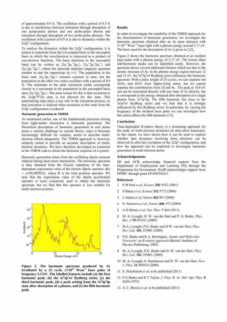
of approximately 0.9 fs. The oscillation with a period of 0.3 fs is due to interference between ionization through absorption of one pump-pulse photon and one probe-pulse photon and ionization through absorption of two probe-pulse photons. The oscillation with a period of 0.9 fs is due to dynamics within the 2s2p2 configuration. To analyse the dynamics within the 2s2p2 configuration, it is easiest to transform from the LS-coupled basis to the uncoupled basis in which the wavefunction is expressed as a product of one-electron functions. The basis functions in the uncoupled basis can be written as |2s0

+2p1+2p0

-, |2s0+2p1

-2p0+, and

|2s0-2p1

+2p0+, where the subscript indicates magnetic quantum

number m and the superscript ms=±½. The population in the basis state |2s0

-2p1+2p0

+ remains constant in time, but the population in the other two states oscillates with a period of 0.9 fs. The minimum in the peak ionization yields corresponds closely to a maximum in the population in the uncoupled basis state |2s0

+2p1+2p0

-. The main reason for this is that excitation to the 2s2p(1Po)3s state is not allowed for this state. This autoionizing state plays a key role in the ionization process, so that ionization is reduced when excitation of this state from the 2s2p2 configuration is reduced. Harmonic generation in TDRM As mentioned earlier, one of the fundamental processes arising from light-matter interaction is harmonic generation. The theoretical description of harmonic generation in real atoms poses a serious challenge to current theory, since it becomes increasingly difficult for complex atoms to describe multi-electron effects adequately. The TDRM approach is, however, uniquely suited to provide an accurate description of multi-electron dynamics. We have therefore developed an extension to the TDRM code to obtain the harmonic response of a system.

Harmonic generation arises from the oscillating dipole moment induced during laser-atom interactions. The harmonic spectrum is thus obtained from the Fourier transform of the time-dependent expectation value of the electric dipole operator, d(t) = -eΨ(t)|R|Ψ(t), where R is the total position operator. We note that the expectation value of the dipole acceleration operator is more commonly used to obtain the harmonic spectrum, but we find that this operator is less suitable for multi-electron systems.

Figure 2. The harmonic spectrum produced by Ar irradiated by a 25 cycle, 2×1013 Wcm-2 laser pulse of frequency 5.17eV. The labelled features include (a) the first harmonic peak, (b) the 3s23p5nℓ Rydberg series, (c) the third harmonic peak, (d) a peak arising from the 3s23p54p state after absorption of a photon, and (e) the fifth harmonic peak.

Results

In order to investigate the suitability of the TDRM approach for the determination of harmonic generation, we investigate the harmonic spectrum obtained after an Ar atom interacts with 2×1013 Wcm−2 laser light with a photon energy around 5.17 eV. The basis used for the description of Ar is given in [12].

Figure 2 shows the harmonic spectrum obtained at an incident laser pulse with a photon energy of 5.17 eV. The lowest three odd-harmonic peaks can be identified easily. However, the spectrum shows several additional features which are due to the atomic structure of Ar. In the photon energy region between 12 and 15 eV, the 3s23p5nℓ Rydberg series influences the harmonic spectrum. With a pulse length of 25 cycles, we can separate out 3d/4s, and 4d/5s from higher-lying states, but we cannot separate the contributions from 3d and 4s. The peak at 18.8 eV can not be associated directly with any state of Ar directly, but it corresponds to the energy obtained after absorption of a single photon from 3s23p54p. The fifth harmonic lies close to the 3s3p6nℓ Rydberg series and we find that it is strongly influenced by this Rydberg series. In particular, by varying the frequency of the incident laser pulse we can investigate how this series affects the fifth harmonic [13].

Conclusions Time-dependent R-matrix theory is a promising approach for the study of multi-electron dynamics on ultra-short timescales. In this report, we have shown how it can be used to explore whether spin dynamics involving three electrons can be observed in ultra-fast excitation of the 2s2p2 configuration, and how the approach can be exploited to investigate harmonic generation in multi-electron atoms

Acknowledgements SH and ACB acknowledge financial support from the Department of Employment and Learning (NI) through the Programme for Government. HvdH acknowledges support from EPSRC through grant EP/G055416/1.

References 1. P M Paul et al, Science 292 5522 (2001)

2. S Baker et al, Science 312 5772 (2006)

3. J. Itatani et al, Nature 432 867 (2004)

4. O. Smirnova et al, Nature 460, 972 (2009)

5. A D Shiner et al, Nat. Phys. 7 464 (2011)

6. M. A. Lysaght, H. W. van der Hart and P. G. Burke, Phys. Rev. A 79 053411 (2009)

7. M.A. Lysaght, P.G. Burke and H.W. van der Hart, Phys. Rev. Lett. 101 253001 (2008)

8. P.G. Burke and K.A. Berrington, Atomic and Molecular Processes: an R-matrix approach (Bristol: Institute of Physics Publishing, 2003)

9. M. A. Lysaght, P.G. Burke and H. W. van der Hart, Phys. Rev. Lett. 102 193001 (2009)

10. M. A. Lysaght, S. Hutchinson and H. W. van der Hart, New J. Phys. 11 093014 (2009)

11. S. Hutchinson et al, to be published (2011)

12. P G Burke and K T Taylor, J. Phys. B: At. Mol. Opt. Phys. 8 2620 (1975)

13. A. C. Brown et al, to be published (2011)

Molecular Dynamics simulations for the viscosity of non-ideal plasmas

Author 1 J. P. Mithen

University of Oxford, Clarendon Laboratory, Parks Road,Oxford, OX1 3PU

Author 2 J. Daligault

Theoretical Division, Los Alamos National Laboratory,Los Alamos, NM, 87545, USA

Author 3 G. Gregori

University of Oxford, Clarendon Laboratory, Parks Road,Oxford, OX1 3PU

Introduction

Viscosity is a fundamental characteristic property of all liquids. Recently, it was shown by the present authors that the viscosity of non-ideal plasmas - which have liquidlike properties - could in principle be measured in x-ray scattering experiments on laser produced plasmas [1]. With this in mind, it is desirable to have theoretical estimates of the viscosity of non-ideal plasmas. In this contribution, we will describe two methods for computing the viscosity and present numerical results.

Both of the methods we describe - the “Green-Kubo method” and the “Hydrodynamic method” - rely on large scale, accurate Molecular dynamics (MD) simulations. In the present instance, these simulations have been performed for the Yukawa system, which is a fluid of particles, mass m , with interaction potential v (r)=(Ze)2 exp(−r /λ s)/4 πϵ0 r . The particles in this system represent interacting ions of charge Ze ; the bare Coulomb interactions between the ions are screened by the electrons. The electronic screening length λ s reduces to either the Debye length or the Thomas-Fermi distance in the limiting cases of classical and degenerate electron fluid respectively [2]. This system, often called the Yukawa one-component plasma (YOCP), is known to be fully characterised by two dimensionless parameters only [3]: the coupling strength

Γ=(Ze)2

(4π ϵ0 kb T ),

where T is the temperature, and the screening parameter

α=aλ s

,

where a=4 n/3−1/3 with n the density. For Γ≥1 , the system represents a 'non-ideal' or 'strongly coupled' plasma; at these coupling parameters the standard results of high temperature plasma physics are no longer applicable. The YOCP represents a highly simplified description of such a non-ideal plasma consisting of ions and electrons. Nevertheless, it is certainly a useful model with which to investigate the properties of these states of matter.

As will be elucidated in the following sections, the viscosity of the YOCP can be calculated by computing its equilibrium dynamics. In order to compute these dynamics we use MD simulations [4]. First, we choose values for Γ and α . For the calculations presented in this contribution, we have chosen a fixed value of α=2 - which is often a reasonable estimate of the screening parameter for a typical non-ideal laser produced plasma - and performed simulations for a range of

Γ values (1, 5, 10, 50, 120 and 175) in order to compute the viscosity for a range of thermodynamic conditions. In our simulations, we perform a long equilibration of duration

1000ωp−1

, where ωp=√n(Ze)2 /ϵ0 m is the plasma

frequency of the system (our timestep is δ t=0.01ωp−1

). After this equilibration, we record the positions and velocities of the N=5000 particles for a further time of

30×819.1ωp−1

. From the particle positions and velocities we can calculate the time-dependent correlation functions

introduced in the following sections (we split the simulation into 30 parts, compute correlation functions for each part, and average in order to improve statistics). Each of the two methods for computing the viscosity, as outlined in the following sections, involves computation of a different time-dependent correlation function.

Green-Kubo method

A standard way to compute the viscosity of a fluid is to use the following “Green-Kubo relation” in which the shear viscosity

η is expressed in terms of the time integral of the shear stress autocorrelation function η(t ) [5],

η=∫0

∞

η(t)dt=1

kB T V∫

0

∞

<σzx(0)σzx(t )>dt . (1)

In Eq. (1), V is the volume of the system (in our case the volume of the simulation box). The brackets <...> denote the usual statistical (thermal) average. The shear stress autocorrelation function is given in terms of the zx component of the microscopic stress tensor,

σzx(t)=∑

i=1

N

[mv i , z(t )v i , x(t)−12 ∑

j=1≠i

N

(zij xij / rij)v(rij)] (2)

where v i , z (t) is the z component of velocity of particlei at time t , and xij=∣x i(t)−x j( t )∣ . Eq. (1) is a

particular example of a “Green-Kubo relation” in which a transport coefficient of a fluid is expressed in terms of a time integral of a microscopic correlation function.

We compute σzx at each timestep using the positions and

velocities from our MD simulations. We can then compute<σ

zx(0)σzx

( t )> by replacing the statistical average by a time average [4], i.e.

<σzx(0)σzx

( t)>=limT→∞

1T∫0

T

σzx(τ)σ

zx( t+τ)d τ . (3)

In this way the shear stress autocorrelation function η(t )appearing in Eq. (1) can be computed. The time integral of

η(t ) then gives the shear viscosity η (see Eq. (1)).

In Fig. 1, we show typical MD results for the normalised shear stress autocorrelation function and the normalised shear viscosity, which are both dimensionless and defined by

η(t )=η(t )/nma2ωp

2 and η=η/nma2ωp respectively.

As shown in Fig. 1, because of noise in the computed shear stress autocorrelation function, the upper limit in the integral in Eq. (1) must be replaced by some cutoff time tcutoff , which is less than the total simulation time of 819.1ωp

−1. We find

that this cutoff time must be chosen differently for each Γ ; the arbitrary choice of tcutoff is a somewhat undesirable necessity of the Green-Kubo method. Despite this, we find that our simulations are long enough that the final result for the viscosity is not particularly sensitive to the choice of tcutoff , providing tcutoff is selected to be close to the time at which

Contact james.mithen@physics.ox.ac.uk

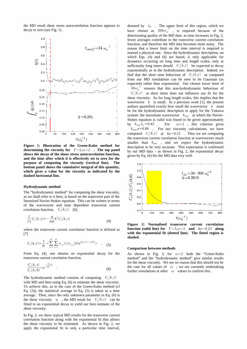
the MD result shear stress autocorrelation function appears to decay to zero (see Fig. 1) .

Hydrodynamic method

The “hydrodynamic method” for computing the shear viscosity, as we shall refer to it here, is based on the transverse part of the linearized Navier-Stokes equation. This can be written in terms of the wavevector and time dependent transverse current correlation function, C t(k ,t ) [6],

∂

∂ tC t(k ,t)=−

η

nmk2 C t(k , t)

(4)

where the transverse current correlation function is defined as [7]

C t(k ,t )=1N

<∑i=1

N

∑j=1

N

v i , x(t )v j , x(0)eik (zi (t)−z j (0))> . (5)

From Eq. (4), one obtains an exponential decay for the transverse current correlation function,

C t(k , t)

C t(k , 0)=e

−η

nmk

2t

. (6)

The hydrodynamic method consists of computing C t(k ,t )with MD and then using Eq. (6) to estimate the shear viscosity. To achieve this, as in the case of the Green-Kubo method (cf Eq. (3)), the statistical average in Eq. (5) is taken as a time average. Then, since the only unknown parameter in Eq. (6) is the shear viscosity η , the MD result for C t(k ,t ) can be fitted to an exponential decay to yield our best estimate of the shear viscosity.

In Fig. 2, we show typical MD results for the transverse current correlation function along with the exponential fit that allows the shear viscosity to be estimated. As shown in Fig. 2, we apply the exponential fit to only a particular time interval,

denoted by t fit . The upper limit of this region, which we have chosen as 200ω p

−1, is required because of the

deteriorating quality of the MD data: as time increases in Fig. 2, fewer averages contribute to the transverse current correlation function, and therefore the MD data becomes more noisy. The reason that a lower limit on the time interval is required is instead a physical one. Since the hydrodynamic description, on which Eqs. (4) and (6) are based, is only applicable for dynamics occurring on long time and length scales, only at sufficiently long times should C t(k ,t ) be expected to decay exponentially as in the hydrodynamic description. Indeed, we find that the short time behaviour of C t(k ,t ) as computed from our MD simulations can be seen to be Gaussian (as expected) rather than exponential. Our chosen lower limit of

50ωp−1

ensures that this non-hydrodynamic behaviour ofC t(k ,t ) at short times does not influence our fit for the

shear viscosity. As for long length scales, this implies that the wavevector k is small. In a previous work [1], the present authors quantified exactly how small the wavevector k must be for the hydrodynamic description to apply for the Yukawa system: the maximum wavevector kmax at which the Navier-Stokes equation is valid was found to be given approximately by kmax λs≈0.43 . For α=2 , this criterion gives

kmax a≈0.86 . For our viscosity calculations, we have computed C t(k ,t ) at ka=0.23 . Thus we are computing the transverse current correlation function at wavevectors much smaller than kmax , and we expect the hydrodynamic description to be very accurate. This expectation is confirmed by our MD data – as shown in Fig. 2, the exponential decay given by Eq. (6) fits the MD data very well.

Comparison between methods

As shown in Fig. 3, for α=2 both the “Green-Kubo method” and the “hydrodynamic method” give similar results for the shear viscosity. We see no reason that this should not be the case for all values of α ; we are currently undertaking further simulations at other α values to confirm this.

Figure 2: Normalised transverse current correlation function (solid line) for Γ=5,α=2 and ka=0.23 along with the exponential fit (dotted line). The fitted region is shaded.

Figure 1: Illustration of the Green-Kubo method for determining the viscosity for Γ=5,α=2 . The top panel shows the decay of the shear stress autocorrelation function, and the time after which it is effectively set to zero for the purpose of computing the viscosity (vertical line). The bottom panel shows the cumulative integral of this quantity, which gives a value for the viscosity as indicated by the dashed horizontal line.

Concluding Remarks

In this contribution we investigated two methods for computing the viscosity of non-ideal plasmas using Molecular Dynamics simulations. As our model of a non-ideal plasma we took the Yukawa one-component plasma. Our work demonstrated that the hydrodynamic method for computing the viscosity is feasible and therefore complements the more widely used method based on the Green-Kubo relation. That is to say, this alternative method provides a way to validate the Green-Kubo result. Furthermore, we expect that in the future our viscosity calculations will be used to assist with the interpretation and analysis of x-ray scattering experiments, which could in principle measure this fundamental physical quantity.

Acknowledgements

This work was supported by the John Fell Fund and by EPSRC grant no. EP/G007187/1.

References

1. J. P. Mithen, J. Daligault and G. Gregori, Phys. Rev. E 83, 015401(R); see also the article “Hydrodynamics of the Yukawa One Component Plasma” (CLF Annual Report 2009-2010).

2. D. Kremp, M. Schlanges and W. D. Kraeft, Quantum Statistics of Nonideal Plasmas (Springer-Verlag, Berlin, 2005).

3. Z. Donkó, G. J. Kalman and P. Hartmann, J. Phys.: Consens. Matter 20, 413101 (2008).

4. See e.g. M. P. Allen and D. J. Tildesley, Computer simulation of liquids (Oxford, New York, 1987).

5. U. Balucani and M. Zoppi, Dynamics of the Liquid State, (Oxford, 1994).

6. J. P. Boon and S. Yip, Molecular Hydrodynamics, (Dover, 1991).

7. J. P. Hansen, I. R. McDonald and E. L. Pollock, Phys. Rev. A 11, 1025 (1975).

Figure 3: Comparison of viscosity as computed by the Green-Kubo method (open circles, with 20% error bars) and the hydrodynamic method (filled triangles).

Kinetic theory of radiation reaction

Adam Noble & Dino Jaroszynski

SUPA & University of Strathclyde,

Glasgow, G4 0NG, UK

Jonathan Gratus & David Burton

Physics Department, Lancaster University, LA1 4YB, UK

& The Cockcroft Institute, Daresbury, UK

Introduction

With the development of ultrahigh intensity laser facilities, such

as the Extreme Light Infrastructure (ELI), it is increasingly

important to understand how charged particles behave in strong

electric and magnetic fields. While it is well known that such

fields cause charges to accelerate, and hence to radiate energy

and momentum, consistently accounting for accelerations

caused by both the applied fields and the radiation field has

troubled physicists for more than a century.

The Abraham-Lorentz-Dirac (ALD) equation, derived to

describe the motion of a radiating point charge, is beset with

difficulties. The worst of these is the existence of solutions

which describe exponentially increasing proper acceleration −

so-called runaway solutions − something at odds with both

intuition and observation.

Because of these problems, many alternative descriptions of

radiation reaction have been proposed. However, the many

independent derivations of the ALD equation suggest it should

remain the starting point of any serious study of radiation

reaction.

Any realistic prospect of studying the effects of radiation

reaction experimentally come from observing not individual

particles, but rather electron bunches containing on the order of

particles or more. It follows that an appropriate description

of radiation reaction is not the single particle ALD equation, but

a kinetic theory based on it. We have recently presented such a

theory, and, after a brief overview of the single-particle theory,

summarize it here.

Single particle theory

The ALD equation for a particle of charge and mass in an

external electromagnetic field is

where is the characteristic time of the particle,

is the projection orthogonal to the 4-velocity

, and an overdot denotes differentiation with respect to

proper time .

The difficulties in using this equation stem from the fact it

involves the derivative of the particle's acceleration, so

specifying initial position and velocity does not uniquely fix the

solution. On the other hand, a generic specification of the

initial acceleration leads to pathological behaviour, with the

proper-acceleration growing exponentially, .

To avoid these problems, Landau and Lifshitz have proposed an

alternative equation of radiation reaction, obtained by

expanding the ALD equation about the Lorentz force:

This equation has the advantage that when the applied force

vanishes, so too does the acceleration, so runaway solutions are

absent. However, while it may be a good approximation for a

single radiating particle, it is far from clear how the errors scale

with the number of particles, so it is not a suitable starting point

for a kinetic theory.

Kinetic theory

For a sufficiently large collection of particles, we can use a

particle distribution function to analyze the average properties,

if we are not concerned with tracking the detailed motion of

each particle.

The Maxwell-Vlasov theory is a self-consistent kinetic theory

of charged particles, which conserves energy and momentum

and so includes some of the bulk features of radiation reaction.

However, it treats the charge as a continuum whose elements

have infinitesimal charge and mass, and so must be altered to

describe particles whose trajectories satisfy the ALD equation.

Since the ALD equation is 3rd order, the appropriate phase

space must have acceleration variables as well as spacetime and

velocity variables. Hence the Liouville vector governing the

dynamics of the system is

where is the 4-acceleration, and is given from the ALD

equation as

Since particles with the same initial conditions evolve together,

the number of particles in a region of phase space remains

constant. It follows that the generalized Vlasov equation takes

the form

where the second term follows from the expansion of the phase

space volume element under the flow of .

This equation governs the motion of the particles. To close the

system, we must couple it to Maxwell's equations, using the

current

Fluid model

The generalized Vlasov equation does not in general reduce to

the usual Vlasov equation in the limit . This is because

any regular solution contains runaway trajectories as well as

physical ones. Hence physical solutions must be singular, with

support only on a submanifold of phase space.

Rather than work with singular quantities, we can take moments

of the generalized Vlasov equation, yielding a fluid theory on

spacetime. Because this procedure involves integrating out the

velocity and acceleration dependence, the moments themselves

are regular, unlike the distribution function.

Define the -moments of the distribution,

Contact adam.noble@strath.ac.uk

where is the invariant measure. Then

integrating the generalized Vlasov equation yields

where parentheses about indices denote symmetrization.

The first few equations read explicitly

where the index denotes the absence of velocity and/or

acceleration terms in the given moments.

It is convenient, and helps to illustrate the relation between the

field system and the original ALD equation, to rewrite the

moment equations in terms of the average velocity and

acceleration,

and the centred moments

where and . Then the above

become

If the centred moments all vanish, these represent the ALD

equation as a field system, with proper time derivatives replaced

by . In general, the centred moments represent collective

effects which drive the average motion away from the motion of

an individual particle.

As with the single particle ALD equation, this field system

contains both physical and unphysical solutions, with the latter

manifesting as instabilities. By analogy with the Landau-

Lifshitz approximation, we can eliminate the unphysical

solutions by expanding the equations about . Because of

the acceleration moments, this will not in general lead to the

same fluid system as we would get from a kinetic theory based

on the Landau-Lifshitz equation.

Reducing a kinetic theory to a fluid system based on a finite

number of modes introduces a loss of information, which

manifests itself in the failure of the moment equations to form a

closed system. It is therefore necessary to introduce equations

of state to supplement the system. Because of the greater

variety of moments available, the appropriate choice of

equation of state is more subtle than for the fluid system based

on the usual Vlasov theory, and further exploration of this issue

is required. One convenient and physically relevant choice

corresponds to a cold fluid model, and involves setting all

centred moments to zero.

Langmuir waves

One of the most fundamental phenomena in the physics of

plasmas is the existence of Langmuir waves, and these provide

an important testing ground for any theory. Although the

effects of radiative damping on such waves will be extremely

small, it provides a useful demonstration of how the theory can

be applied. For simplicity, we consider only the case of a cold

plasma.

The equilibrium state for a cold quiescent plasma is

with external current due to the ions,

.

Linearizing the field system and Maxwell's equations about this

equilibrium, and seeking harmonic longitudinal solutions of

frequency leads to the dispersion relation

where is the plasma frequency. This has three

roots: two (physically equivalent) physical solutions,

and the unphysical solution,

The physical roots behave as one would expect: oscillations

close to the plasma frequency, with a small radiative damping

term. The third root describes an extremely rapid growth

without oscillation. Its origin in the runaway solutions of the

ALD equation is seen in the impossibility of taking the limit

, so it must be rejected as unphysical.

Conclusions

We have discussed a kinetic theory suitable for describing large

numbers of radiating electrons, based on the exact Abraham-

Lorentz-Dirac equation. Like the ALD equation, it admits both

physical solutions and unphysical ones for which the limit

does not exist.

While the presence of the nonphysical solutions prevents the

kinetic theory from reducing to the usual Maxwell-Vlasov

description in the appropriate limit, a fluid model can be

derived from the moments of the particle distribution function

which does have the correct correspondence limit.

As a simple demonstration of the theory, we have applied it to

the radiative damping of Langmuir waves, and found that, as

expected, it exhibits both physically reasonable behaviour and

unphysical solutions which must be rejected.

Acknowledgements

We acknowledge the support of the U. K. EPSRC, the Laserlab-

Europe consortium and the FP7 - Extreme Light Infrastructure

(ELI) project.

References

1. P.A.M. Dirac, Proc. R. Soc. A 167 148 (1938)

2. L.D. Landau and E.M. Lifshitz, The Classical Theory of

Fields (Pergamon, London, 1962)

3. A. Noble et al., Proc. SPIE 8079, 80790L (2011)

4. A. Noble et al., A kinetic model of radiating electrons, in

preparation.

Simulating Prolific Pair-Production in 10PW Laser-Plasma Interactions

C. P. Ridgers

University of Oxford Clarendon Laboratory, Parks Road, Oxford, OX1 3PU

A. R. Bell

University of Oxford & Rutherford Appleton Laboratory Clarendon Laboratory, Parks Road, Oxford, OX1 3PU

J. G. Kirk

Max Planck-Institute fur Kernphysik Postfach 10 39 80, 69029 Heidelberg, Germany

R. Duclous

Commissariat a l’Energie Atomique, Bruyeres-le-Chatel, DAM-Ile de France, France

Introduction

With the next generation of high intensity lasers it will be possible to access the regime in which Quantum Electrodynamics (QED) plays an important role. Specifically, the laser-fields may be sufficiently strong to generate electron-positron pairs [1,2]. In order to correctly simulate laser-plasma interactions with 10PW lasers one must include pair production in the modeling tools, first and foremost in Particle-in-Cell (PIC) codes. Here we will discuss the model required to do this efficiently.

At laser intensities between 1023Wcm-2 and 1024Wcm-2 two effects become increasingly important. Firstly the acceleration of the electrons in the laser fields is sufficiently violent that they may generate high-energy gamma-ray photons, the generation of which causes the electron to recoil significantly. This radiation drag is important in determining the motion of the electrons. The high energy photons may then go on to generate pairs in the fields of the laser, a process known as the (multiphoton) Breit-Wheeler process. Alternatively the electrons may generate pairs directly in the laser-fields, via a virtual photon. This is known as the Trident process. Of particular interest is the fact that the two-step Breit-Wheeler process can lead to all of the laser energy being converted to pairs, and so very efficient antimatter production [1,3]. At 10PW laser intensities the emission of gamma rays by the electrons is discontinuous, i.e. few high-energy photons are emitted instead of continuous radiation. This enhances the rate of pair production as the electron can reach high energy between emission events and so emit a high energy photon which is in turn more likely to create a pair, this process is known as straggling [4].

The theoretical model

A semi-classical model describing the QED effects described above was developed by Bell, Kirk, Arka & Duclous [1,2,4], a summary of this model is presented here.

The controlling parameter determining the rate of emission of photons by electrons accelerated in the laser fields is

η = γ E⊥

Es

+ v ×BBs

(1)

Here E⊥ is the electric field perpendicular to the direction of motion of the electron Es (= cBs =1.3x1018Vm-1) is the Schwinger field (the field at which the vacuum breaks down into a cascade of pairs). Pair production becomes important when η becomes of the order of 0.1 [1]. For an intensity of 1023Wcm-2 the electric field of the laser is of the order of 1015Vm-1. From equation (1) one can see that when the

Lorentz factor of the electrons (γ) is of the order of 100 then pairs should be produced in significant quantities. Electrons are accelerated to this energy by a 10PW laser.

The second controlling parameter is

χ =hν

2mec2

E⊥

Es

+kk

×BBs

(2)

Here hν is the relevant photon energy and k is its wavevector.

The rate of generation of gamma-ray photons by an electron and their energy are controlled by these parameters. The rate of generation of photons of all energies by a single electron of Lorentz factor γ is

dNγ

dt= 3

mec2α f

hηγ

F(η,χ)χ0

η / 2

∫ dχ (3)

Where η and γ are those for the emitting electron. F(η,χ) is the (quantum-corrected) synchrotron function [2]. As the energy of the electron increases, the energy spectrum (i.e. the synchrotron function) shifts to higher energies, and so higher energy photons are emitted; these are much more likely to generate pairs.

The rate of pair production from photons with energy hν and controlling parameter χ by the Breit-Wheeler process is given by

dN±

dt=

α f mec2

hmec

2

hνχT(χ) (4)

The corresponding rate of pair production directly by an electron (the Trident process) with Lorentz factor γ and controlling parameter η is

dN±

dt= 0.64

α f2mec

2

hηγ

Ω(η) (5)

Ω(η) and T(χ) are well known functions [2,5].

The inclusion of pair production in PIC codes

The emission of gamma-ray photons and pairs described above is a statistical process. A quantum particle may or may not emit in a given time interval subject to emission probabilities. This statistical nature of the emission process gives rise to the straggling effect already mentioned [4]. In order to capture this effect a Monte-Carlo approach is taken when including pair-production in a PIC code [4]. If a beam of particles of initial intensity I0 travels through a medium of optical depth τ then the emerging intensity is

Contact c.ridgers1@physics.ox.ac.uk

I = I0e−τ ⇒ P = (1− e−τ ) (6)

P is probability of a given beam particle emitting. From equation (6) we see that most particles penetrate to some small optical depth, with relatively fewer getting further. Such a description of the emission process is naturally suited to inclusion in a PIC code. Each particle is assigned with a P-value at random, this is used to compute the optical depth it reaches before emission. As the particle moves along its worldline by distance ∆s, ∆τ is added to its optical depth until it reaches its optical depth for emission, at which point it emits a particle. The increments to the optical depth are

∆τ = ∆tdNdt

(7)

dN/dt is the relevant rate of particle production, for the generation of photons by an electron or positron this is given by equation (3) and for the generation of a pair from a photon by equation (4). Note that it has been shown that the generation of pairs by the Trident process is not important for high intensity (>3x1023Wcm-2) interactions and it will no longer be considered [4].

We will now consider each step in the two-step Breit-Wheeler process. Firstly a photon is generated. This occurs when the optical depth of an electron or positron equals that for emission as calculated using the Monte-Carlo approach described above. The photon is emitted moving in the same direction as the electron or positron, its energy is determined by a quantum, and therefore, Monte-Carlo process. The probability that the emitted photon has a given energy is set by the synchrotron function. The energy of the photon is related to the χ-value with which it is emitted. The probability of the photon having a χ-value between 0 and χf is

P =

d2Nγ

dχdtdχ

0

χ f

∫d2Nγ

dχdtdχ

0

η / 2

∫=

F(η,χ)χ

dχ0

χ f

∫F(η,χ)

χdχ

0

η / 2

∫ (8)

Once again P is chosen at random and by inverting equation (8) χf is found. This then gives the energy of the emitted photon

hν =2mec

2χ f γη

(9)

η and γ are those for the emitting particle.

The electron (or positron) recoils, resulting in its momentum changing from pf to pi

p f = pi −h

2πk (10)

k is the wavevector of the emitted photon. This formulation does not conserve energy but the error has been shown to be of the order of 1/γiγf (the subscripts i and f denote the initial and final states of the electron respectively) [4]. The error is small as the electron is ultra-relativistic in 10PW laser-plasma interactions.

The photon generated is then assigned an optical depth for emission and propagates until this is reached, at which point it emits a pair and is annihilated. The electron and positron are emitted moving in the same direction as the photon. The electron is assigned a fraction of the photon’s energy f. The probability of the electron gaining this fraction is given by

P =

dR( f ,χ)df

df0

f

∫dR( f ,χ)

dfdf

0

1

∫ (11)

dR(f,χ)/df is given by [6]

dR( f ,χ)df

∝2 + f (1− f )

f (1− f )K2 / 3

13χf (1− f )

(12)

Where χ is that for the emitting photon and K2/3 is a Bessel function of the second kind. The constant in equation (12) is not required as P is expressed as a ratio.

The electron is assigned a P-value at random and equation (11) is inverted to determine f. It should be noted that the value of f is relatively unimportant as the energy the electron and positron in the pair gain by acceleration in the laser field is typically much greater than that they start with.

Conclusions

A relatively straightforward prescription for including radiation and pair-production in a PIC code has been developed and presented here in summary. Including these QED effects is of crucial importance to modeling the interaction of 10PW laser-plasma interactions, where such processes are of importance.

References

[1] A.R.Bell & J.G.Kirk, Phys Rev Lett, 101, 200403 (2008)

[2] J.G.Kirk, A.R.Bell & I.Arka, Plas Phys Cont Fus, 51, 085008 (2009)

[3] N.Elkina et al, Phys.Rev.ST Accel.Beams, 14, 054401 (2011)

[4] R.Duclous, Plas Phys Cont Fus, 53, 015009 (2010)

[5] T.Erber, Rev Mod Phys, 38, 629 (1966)

[6] J.K.Daugherty & A.K.Harding, Ap J, 273, 761 (1983)

The Magnetic Switchyard : Guiding Fast Electrons for Fast Ignition ICF

A.P.L.Robinson

Central Laser Facility STFC Rutherford-Appleton Laboratory Didcot, OX11 0QX, United Kingdom

M.Tabak and M.H.Key

Lawrence Livermore National Laboratory Livermore USA

Introduction

Fast Ignition ICF [1] is an attractive alternative to central hot-spot ignition of inertially confined fusion fuel. The key attractions are the significant reductions in implosion requirements and the overall reduction in laser energy that should be required (a few hundred kJ as opposed to > 1MJ).

The reduction in overall laser energy will only be achieved if there is a sufficiently high coupling efficiency between the short “ignitor” laser pulse and the hot spot that is generated in the compressed DT fuel. Extensive hydrodynamic studies, based on analytic considerations, have indicated that the minimum energy that must be coupled into the hot spot for ignition are in the range 10-20kJ (assuming DT compressed to 350-400 gcm-

3) in 10-20ps. Achieving a laser to fast electron conversion efficiency of 30%, and perhaps higher, is not unlikely. This therefore leaves the question of how to ensure that a sufficiently large proportion of the fast electron energy is deposited in the hot spot. If the fast electron population has a large divergence angle (PIC simulations increasingly suggest this is the case) this will not be possible, but if one could devise a scheme for effectively guiding the fast electrons then this could become possible.

In this report we describe a new concept for guiding fast electrons using structured inserts in the cone tip. The concept has been assessed using 3D numerical simulations for multi-kJ conditions that are relevant to full Fast Ignition.

Magnetic Switchyard Concept

We propose a new concept for effectively guiding the fast electrons in the case where the fast electrons have a high divergence angle. This is termed the “Magnetic Switchyard”, and this is based on the idea of engineering the growth of resistivity gradients that the authors proposed in [2], and which were explored experimentally in [3,4]. The idea is to use an insert in cone and to focus the laser onto the rear surface of the insert. The insert consists of an array of concentric quasi-cylindrical shells embedded in a lower-Z substrate. The shells are axisymmetric about the cone axis. This arrangement is illustrated in figure 1 below.

Figure 1 : Slice Plot of Z for a Magnetic Switchyard insert into a cone. Red regions are higher Z than blue regions. This shows the concentric, axisymmetric shells embedded in the lower-Z material.

The Magnetic Switchyard works as follows : As fast electrons flow through the structure, initially as a divergent spray, magnetic fields will grow at the interfaces between higher-Z and lower-Z materials. These fields will act to push fast electrons into the higher-Z guiding shells. Eventually the magnetic fields will have grown to such an extent that they will function as `rigid pipes’ for the fast electrons. The shells will only accept a part of the fast electron source with a limited angular spread. As the bunches move through the shell they will have their mean direction altered (from diverging to converging), but the angular spread of the bunch cannot be reduced. At the far end of the switchyard we should thus emit electron bunches whose mean direction have all been altered so as to point at a distant target region. In a fast ignition scenario there is now no need to introduce any guiding elements outside the cone, which pose problems for hydrodynamic fuel assembly. In figure 2 below, we show the results of a 2D particle tracking simulation through a prescribed B-field arrangement similar to what one might obtain. This shows how such an arrangement might act to guide electrons.

Figure 2. Results of 2D particle tracking calculation through a prescribed B-field. This illustrates how the Switchyad might work to guide fast electrons to a distant point, even when they are initially divergent.

3D Hybrid Simulation Model

In what follows we will now show the results of one of a number of numerical simulations that show that the magnetic switchyard concept may be highly beneficial to Fast Ignition ICF, even if the switchyard is not too complex.

The numerical simulations are 3D particle-based hybrid code calculations, that have been performed using the ZEPHYROS code [3,4]. ZEPHYROS is a particle hybrid code, and a description of this method can be found in the work of Davies and co-workers [5]. The simulations were performed on a 200x200x200 grid with a cell size of 1µm on each side. In these simulations an array of carbon shells (density 2gcm-3)

Contact alex.robinson@stfc.ac.uk

embedded in CH2 (density of 1gcm-3) was studied. The atomic Z-map and ion density are shown in figure 3 below as a slice through the x-y mid-plane. The background temperature is initially set to 100eV. Note that we also include compressed DT fuel in the simulation, however no hydrodynamics or burn is included in the simulation model.

The fast electron injection models irradiation by a laser intensity of 4 x 1020Wcm-2 with a 50% conversion efficiency. The temporal profile of the beam is a top-hat function of 18ps duration, and the transverse injection profile that was employed is exp(-(r/rs)

4) with rs = 15µm . The fast electron distribution was given by a single-temperature relativistic Maxwellian in energy, with Tf = 2.6MeV (from the ponderomotive scaling with a 0.351µm wavelength) and in terms of angular distribution a uniform distribution over a cone subtended by a half-angle of 70o was used. The total fast electron energy that is injected is 23kJ. These simulations are run up to 20ps.

Figure 3 : Ion Charge (Z) in x-y midplane (left), and Ion Density in x-y midplane (right).

Results

In the simulation it was found that the Magnetic Switchyard structure had a strong guiding effect on the fast electrons as we anticipated. In figure 4 we show the fast electron density and the Bz component of the magnetic flux density in the x-y midplane at 6ps.

Figure 4 : Fast Electron Density in x-y midplane at 6ps (left), and Bz component of magnetic flux density in x-y midplane at 6ps (right).

The fast electron density in figure 4 shows that strong guiding of the fast electrons has occurred, both through the switchyard structure and through the DT fuel. The structure of the fast electron density is interesting. There exists a distinct cone that suggests convergence of fast electrons, surrounded by a ‘penumbra’ of lower fast electron density, which suggests that it consists of divergent fast electrons.

The plot of Bz in figure 4 shows that collimating/confining B-field builds up around all of the more resistive shells inside the Switchyard as expected, thus achieving the anticipated effect. In the DT fuel region we note that a strong collimating field is generated but only around the aforementioned ‘penumbral’ part of the fast electron beam. The denser, converging part of the beam only seems to have much weaker magnetic field associated with it.

The observations of the fast electron density pattern and magnetic field apply to most of the simulation time. At the end

of the simulation, one is clearly more interested in examining the coupling of the fast electron energy into the dense DT fuel.

Figure 5 : Ion temperature in x-y midplane at 20ps (left), and Ion Internal Energy in x-y midplane at 20ps (right). Note that both plots only show the DT fuel region.

In figure 5 we show plots of the ion temperature and ion internal energy at 20ps in the DT fuel region only (i.e. > 110 µm). In terms of the energetic of this simulation, it is important to remember that 23kJ of fast electron energy is injected. The ion temperature shows that a very small spot is heated to 6keV (at this point the density is about 275gcm-3) and this is surrounded by a wider region which is heated to about 3keV. In terms of the ion internal energy one can see that a roughly spherical hot spot has been generated with a roughly 20µm radius. If one integrates the internal energy over a 40x40x40µm cube centred on (172,100,100)µm then one finds that 6.22kJ has been deposited. This means that the effective coupling efficiency is 27%. The Atzeni minimum ignition criterion [6] for a spot of this size would be about 22kJ so this is insufficient to ignite the target. Nonetheless it does show that the Switchyard can lead to good coupling efficiencies even when the electron divergence is large (70o half-angle in this case) under multi-kJ Fast Ignition relevant conditions.

Conclusions

In this article we have reported on the development of a new concept for guiding fast electrons which are initially highly divergent for Fast Ignition ICF. The concept is based on previous work which showed that resistivity gradients can be used to engineer the growth of collimating magnetic field as required. 3D hybrid simulations suggest that even when the electron divergence half-angle is 70o, that the use of the switchyard results in 27% coupling into a 20µm radius hot-spot. Future work will concentrate on scaling the concept to full ignition conditions.

Acknowledgements

APLR is grateful for the use of computing resources provided by Science and Technology Facilities Council's e-Science facility.

APLR would like to thank A.R.Bell, W.Bokee-West, M.Tolley, and P.A.Norreys for their advice and useful discussions during the course of this work.

References

1. M.Tabak et al., Phys.Plasmas, 1 (1994)

2. A.P.L.Robinson and M.Sherlock, Phys.Plasmas, 14, 083105 (2007)

3. S.Kar et al., Phys.Rev.Lett., 102, 055001 (2009)

4. B.Ramakrishna et al., Phys.Rev.Lett., 105, 135001(2010)

5. J.R.Davies et al, Phys.Rev.E, 56 (1997)

6. S.Atzeni, Phys.Plasmas, 6 , 3316 (1999)

Production of high energy protons with hole-boring radiation pressure acceleration

A.P.L.Robinson

Central Laser Facility, STFC Rutherford-Appleton Laboratory Didcot, Oxfordshire, United Kingdom OX11 0QX

Introduction

Recently there has been considerable interest in Radiation Pressure Acceleration (RPA) of ions. RPA can occur in two distinct modes that have been termed ‘Light Sail’ (LS) [1] and ‘Hole-Boring’ (HB) [2] RPA respectively. In LS RPA a slab of plasma will be accelerated as a whole, and it has been shown that numerical simulations of this are well modeled by the classic simple model of a planar reflecting slab being accelerated by pure light pressure – hence the name. In HB RPA a laser pulse will drive into a thick slab of plasma pushing a beam of ions ahead of the receding plasma surface. Studies suggest that it should be much easier to reach high energies (> 100MeV per nucleon) with LS RPA than HB RPA.

In non-relativistic HB RPA the ion energy should be given by ,

,cn

I

i

=ε (1)

and if we now assume that the minimum ion density is a0nc, then we can express the intensity in terms of a0 and substitute to obtain,

20 cma e=ε , (2)

which is a very slow scaling compared to LS RPA. This scaling is not consistent with previous numerical simulations which show a much better scaling [2]. In this article we will examine why Eq. 2 is incorrect, and thus show that HB-RPA is much less restricted than the a0nc ‘limit’ suggests. This opens up the possibility that HB RPA will actually allow us to produce 100-200MeV protons at not excessively high intensities.

Theory

The a0nc ‘limit’ on HB-RPA comes from the minimum density at which a plasma will be transparent to an incident laser pulse. Linearized relativistic fluid theory gives this as a0nc for the case of a circularly polarized laser pulse. The problem with this is that linear theory does not fully treat such high intensity laser-plasma interactions. The effect of non-linearity on the penetration of laser pulses into plasma slabs was thoroughly analysed by Cattani et al. [3] using analytic theory. This yields the following expression for the penetration threshold at a given a0,

[ ],)11)(1(241 4222

dddp aaana −−++= (3)

where,

,1169

23

189 22

+−+−= nnnnad (4)

Note that the electron density is normalized to the critical density in Eq.3 and 4. If this is shown graphically, as is done in figure 1, then we find that the penetration threshold rapidly exceeds that predicted by linear theory. In other words, Cattani’s analysis indicates that we should be able to achieve HB-RPA with much lower density plasmas than that predicted by linear theory.

Figure 1 : Penetration threshold in terms of a0 as predicted by Eq. 3 and 4.

Futhermore we can use the expressions developed in [2] to predict the proton energies that can be achieved given this limit. If one assumes that the laser wavelength is 1µm and that HB-RPA can be achieved right at the penetration threshold then one obtains the curves plotted in figure 2 below where both the maximum obtainable energy and the intensity requirement are plotted.

This shows that protons in the range of 100-200MeV can be generated using laser intensities in the range of 5x1021-1x1022 Wcm-2. In [2] the PIC simulations suggested that one would need 2-4x1022 Wcm-2 to reach the 100-200MeV so this result represents a reduction by a factor of four in the required intensity. In what follows we will report on our numerical investigations that were carried out to validate this theoretical result.

Contact A.P.L.Robinson@stfc.ac.uk

Figure 2 : Maximum achievable proton energy from HB-RPA as a function of plasma density normalized to critical density at 1µm wavelength.

Numerical Simulation Set-Up

One dimensional electromagnetic Particle-in-Cell simulations were carried out to address the questions raised in the preceding section. The code employed for this is the same used in previous investigations (e.g. [1]).The plasma consists of a purely hydrogenic plasma initially at a temperature of 20keV with a density in the range 3-10x1027m-3. The plasma has a `top-hat' density profile and is 10µm thick. Each species is represented by 100 macroparticles per cell. The spatial grid consisted of 10000 cells of 10nm width. A circularly polarized pulse with a FWHM intensity of IFWHM = 1.25 x 1021Wcm-2 and FWHM duration of 40fs is incident on the target from the left. The pulse has a sin2 temporal profile and a wavelength of 1µm.

Results

Initially a scan was conducted over the range of densities from 3-10x1027m-3 and the results are summarized in figure 3 in which we show the average energy of the protons accelerated by HB RPA at 75fs (if any), and the predicted energy according to the formulae of [2] for both the FWHM intensity and the peak intensity. As can be seen, we are obtaining HB RPA at plasma densities well below a0nc as predicted. To demonstrate that HB RPA is indeed observed we show the results of one particular simulation (the one where n = 7x1027m-3) in figure 4. This clearly shows the hole-boring process in the both the phase space, and the strong pistoning of the plasma in terms of the particle densities. Note that the actual target thickness is not important provided that it is more than a few microns thick. The target could be much thicker than the 10µm used here and the same results would be obtained.

Figure 3 : Results of 1D PIC simulation as average proton versus plasma density (blue circles). Black line is predicted proton energy from HB formulae at FWHM intensity and red line is the same at the peak intensity.

Figure 4 : (Left) px-x phase space for protons. (Right) Number densities of protons (red) and electrons (blue). Data is taken from the n = 7x1027m-3 simulation.

The loss of HB-RPA at 6x1027m-3 is consistent with Cattani’s prediction for the penetration threshold. On extending this method of scanning across density at a given a0 to a set of a0s we have found a very good general agreement with Cattani’s prediction.

Thus 1D PIC simulations validate the idea that one can reach much higher proton energies using HB-RPA than one would think from the a0nc limit.

This is the main text of the article. This will include many lines about what the article is about. There can be many sections depending what the subject matter is. These may contain graphs, figures, photos equations etc.

Conclusions

In this paper we addressed the question of the minimum plasma density that can be used to obtain HB-RPA. If this were limited to a0nc then reaching high proton energies is demanding. We showed, however, that the limit is considerably lower due to the effect of nonlinear processes on laser pulse penetration. In fact this reduces the intensities required to reach the 100-200MeV range by a factor of 4 – down to 0.5-1x1022Wcm-2, which means that high energy proton generation from HB-RPA should be possible. In future we will conduct multi-dimensional simulations to further investigate this route.

References

1. T.Esirkepov, Phys.Rev.Lett., 92, 175003-1 (2004)

2. A.P.L.Robinson, Plasma Phys.Control. Fusion, 51, 024004 (2009)

3. F.Cattani et al., Phys.Rev.E, 62, 1234 (2000)

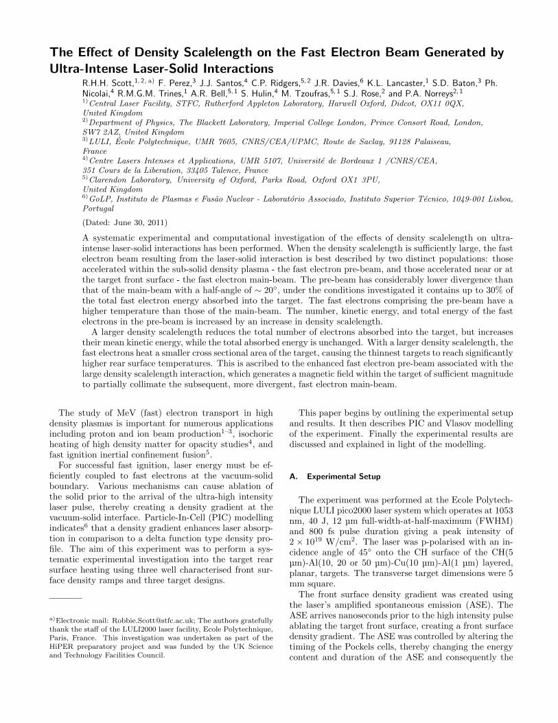
The Effect of Density Scalelength on the Fast Electron Beam Generated byUltra-Intense Laser-Solid Interactions

R.H.H. Scott,1, 2, a) F. Perez,3 J.J. Santos,4 C.P. Ridgers,5, 2 J.R. Davies,6 K.L. Lancaster,1 S.D. Baton,3 Ph.Nicolai,4 R.M.G.M. Trines,1 A.R. Bell,5, 1 S. Hulin,4 M. Tzoufras,5, 1 S.J. Rose,2 and P.A. Norreys2, 11)Central Laser Facility, STFC, Rutherford Appleton Laboratory, Harwell Oxford, Didcot, OX11 0QX,United Kingdom2)Department of Physics, The Blackett Laboratory, Imperial College London, Prince Consort Road, London,SW7 2AZ, United Kingdom3)LULI, Ecole Polytechnique, UMR 7605, CNRS/CEA/UPMC, Route de Saclay, 91128 Palaiseau,France4)Centre Lasers Intenses et Applications, UMR 5107, Universite de Bordeaux 1 /CNRS/CEA,351 Cours de la Liberation, 33405 Talence, France5)Clarendon Laboratory, University of Oxford, Parks Road, Oxford OX1 3PU,United Kingdom6)GoLP, Instituto de Plasmas e Fusao Nuclear - Laboratorio Associado, Instituto Superior Tecnico, 1049-001 Lisboa,Portugal

(Dated: June 30, 2011)

A systematic experimental and computational investigation of the effects of density scalelength on ultra-intense laser-solid interactions has been performed. When the density scalelength is sufficiently large, the fastelectron beam resulting from the laser-solid interaction is best described by two distinct populations: thoseaccelerated within the sub-solid density plasma - the fast electron pre-beam, and those accelerated near or atthe target front surface - the fast electron main-beam. The pre-beam has considerably lower divergence thanthat of the main-beam with a half-angle of ∼ 20, under the conditions investigated it contains up to 30% ofthe total fast electron energy absorbed into the target. The fast electrons comprising the pre-beam have ahigher temperature than those of the main-beam. The number, kinetic energy, and total energy of the fastelectrons in the pre-beam is increased by an increase in density scalelength.

A larger density scalelength reduces the total number of electrons absorbed into the target, but increasestheir mean kinetic energy, while the total absorbed energy is unchanged. With a larger density scalelength, thefast electrons heat a smaller cross sectional area of the target, causing the thinnest targets to reach significantlyhigher rear surface temperatures. This is ascribed to the enhanced fast electron pre-beam associated with thelarge density scalelength interaction, which generates a magnetic field within the target of sufficient magnitudeto partially collimate the subsequent, more divergent, fast electron main-beam.

The study of MeV (fast) electron transport in highdensity plasmas is important for numerous applicationsincluding proton and ion beam production1–3, isochoricheating of high density matter for opacity studies4, andfast ignition inertial confinement fusion5.

For successful fast ignition, laser energy must be ef-ficiently coupled to fast electrons at the vacuum-solidboundary. Various mechanisms can cause ablation ofthe solid prior to the arrival of the ultra-high intensitylaser pulse, thereby creating a density gradient at thevacuum-solid interface. Particle-In-Cell (PIC) modellingindicates6 that a density gradient enhances laser absorp-tion in comparison to a delta function type density pro-file. The aim of this experiment was to perform a sys-tematic experimental investigation into the target rearsurface heating using three well characterised front sur-face density ramps and three target designs.

a)Electronic mail: Robbie.Scott@stfc.ac.uk; The authors gratefullythank the staff of the LULI2000 laser facility, Ecole Polytechnique,Paris, France. This investigation was undertaken as part of theHiPER preparatory project and was funded by the UK Scienceand Technology Facilities Council.

This paper begins by outlining the experimental setupand results. It then describes PIC and Vlasov modellingof the experiment. Finally the experimental results arediscussed and explained in light of the modelling.

A. Experimental Setup

The experiment was performed at the Ecole Polytech-nique LULI pico2000 laser system which operates at 1053nm, 40 J, 12 µm full-width-at-half-maximum (FWHM)and 800 fs pulse duration giving a peak intensity of2 × 1019 W/cm2. The laser was p-polarised with an in-cidence angle of 45 onto the CH surface of the CH(5µm)-Al(10, 20 or 50 µm)-Cu(10 µm)-Al(1 µm) layered,planar, targets. The transverse target dimensions were 5mm square.

The front surface density gradient was created usingthe laser’s amplified spontaneous emission (ASE). TheASE arrives nanoseconds prior to the high intensity pulseablating the target front surface, creating a front surfacedensity gradient. The ASE was controlled by altering thetiming of the Pockels cells, thereby changing the energycontent and duration of the ASE and consequently the

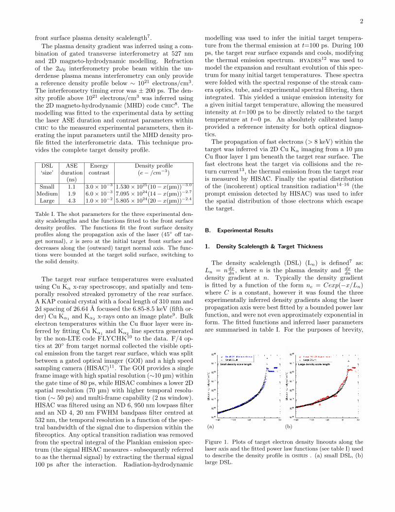
2

front surface plasma density scalelength7.

The plasma density gradient was inferred using a com-bination of gated transverse interferometry at 527 nmand 2D magneto-hydrodynamic modelling. Refractionof the 2ω0 interferometry probe beam within the un-derdense plasma means interferometry can only providea reference density profile below ∼ 1021 electrons/cm3.The interferometry timing error was ± 200 ps. The den-sity profile above 1021 electrons/cm3 was inferred usingthe 2D magneto-hydrodynamic (MHD) code chic8. Themodelling was fitted to the experimental data by settingthe laser ASE duration and contrast parameters withinchic to the measured experimental parameters, then it-erating the input parameters until the MHD density pro-file fitted the interferometric data. This technique pro-vides the complete target density profile.

DSL ASE Energy Density profile‘size’ duration contrast (e− /cm−3)

(ns)Small 1.1 3.0 × 10−3 1.530 × 1025(10 − x(µm))−3.0

Medium 1.9 6.0 × 10−3 7.095 × 1024(14 − x(µm))−2.7

Large 4.3 1.0 × 10−2 5.805 × 1024(20 − x(µm))−2.4

Table I. The shot parameters for the three experimental den-sity scalelengths and the functions fitted to the front surfacedensity profiles. The functions fit the front surface densityprofiles along the propagation axis of the laser (45 off tar-get normal), x is zero at the initial target front surface anddecreases along the (outward) target normal axis. The func-tions were bounded at the target solid surface, switching tothe solid density.

The target rear surface temperatures were evaluatedusing Cu Kα x-ray spectroscopy, and spatially and tem-porally resolved streaked pyrometry of the rear surface.A KAP conical crystal with a focal length of 310 mm and2d spacing of 26.64 A focussed the 6.85-8.5 keV (fifth or-der) Cu Kα1

and Kα2x-rays onto an image plate9. Bulk

electron temperatures within the Cu fluor layer were in-ferred by fitting Cu Kα1

and Kα2line spectra generated

by the non-LTE code FLYCHK10 to the data. F/4 op-tics at 20 from target normal collected the visible opti-cal emission from the target rear surface, which was splitbetween a gated optical imager (GOI) and a high speedsampling camera (HISAC)11. The GOI provides a singleframe image with high spatial resolution (∼10 µm) withinthe gate time of 80 ps, while HISAC combines a lower 2Dspatial resolution (70 µm) with higher temporal resolu-tion (∼ 50 ps) and multi-frame capability (2 ns window).HISAC was filtered using an ND 6, 950 nm lowpass filterand an ND 4, 20 nm FWHM bandpass filter centred at532 nm, the temporal resolution is a function of the spec-tral bandwidth of the signal due to dispersion within thefibreoptics. Any optical transition radiation was removedfrom the spectral integral of the Plankian emission spec-trum (the signal HISAC measures - subsequently referredto as the thermal signal) by extracting the thermal signal100 ps after the interaction. Radiation-hydrodynamic

modelling was used to infer the initial target tempera-ture from the thermal emission at t=100 ps. During 100ps, the target rear surface expands and cools, modifyingthe thermal emission spectrum. hyades12 was used tomodel the expansion and resultant evolution of this spec-trum for many initial target temperatures. These spectrawere folded with the spectral response of the streak cam-era optics, tube, and experimental spectral filtering, thenintegrated. This yielded a unique emission intensity fora given initial target temperature, allowing the measuredintensity at t=100 ps to be directly related to the targettemperature at t=0 ps. An absolutely calibrated lampprovided a reference intensity for both optical diagnos-tics.

The propagation of fast electrons (> 8 keV) within thetarget was inferred via 2D Cu Kα imaging from a 10 µmCu fluor layer 1 µm beneath the target rear surface. Thefast electrons heat the target via collisions and the re-turn current13, the thermal emission from the target rearis measured by HISAC. Finally the spatial distributionof the (incoherent) optical transition radiation14–16 (theprompt emission detected by HISAC) was used to inferthe spatial distribution of those electrons which escapethe target.

B. Experimental Results

1. Density Scalelength & Target Thickness

The density scalelength (DSL) (Ln) is defined7 as:Ln = n dxdn , where n is the plasma density and dx

dn thedensity gradient at n. Typically the density gradientis fitted by a function of the form ne = Cexp(−x/Ln)where C is a constant, however it was found the threeexperimentally inferred density gradients along the laserpropagation axis were best fitted by a bounded power lawfunction, and were not even approximately exponential inform. The fitted functions and inferred laser parametersare summarised in table I. For the purposes of brevity,

(a) (b)

Figure 1. Plots of target electron density lineouts along thelaser axis and the fitted power law functions (see table I) usedto describe the density profile in osiris . (a) small DSL, (b)large DSL.

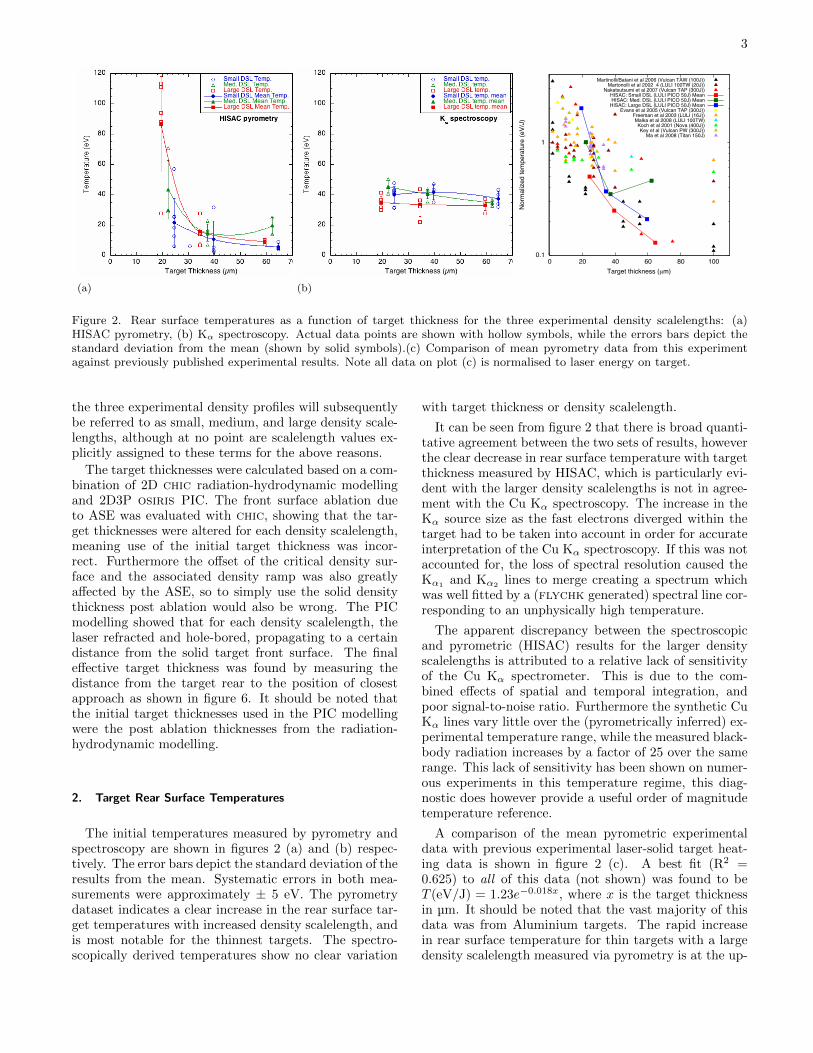
3

(a) (b)

0.1

1

0 20 40 60 80 100

Norm

alize

d te

mpe

ratu

re (e

V/J)

Target thickness (µm)

Target rear surface temperature normalized to laser energy

Martinolli/Batani et al 2006 (Vulcan TAW (100J))Martonolli et al 2002 4 (LULI 100TW (20J))

Nakatsutsumi et al 2007 (Vulcan TAP (300J))HISAC: Small DSL (LULI PICO 50J) MeanHISAC: Med. DSL (LULI PICO 50J) Mean

HISAC: Large DSL (LULI PICO 50J) MeanEvans et al 2005 (Vulcan TAP (300J))

Freeman et al 2003 (LULI (16J))Malka et al 2008 (LULI 100TW)Koch et al 2001 (Nova (400J))Key et al (Vulcan PW (300J))

Ma et al 2008 (Titan 150J)

0.1

1

0 20 40 60 80 100

Norm

alize

d te

mpe

ratu

re (e

V/J)

Target thickness (µm)

Target rear surface temperature normalized to laser energy

Martinolli/Batani et al 2006 (Vulcan TAW (100J))Martonolli et al 2002 4 (LULI 100TW (20J))

Nakatsutsumi et al 2007 (Vulcan TAP (300J))HISAC: Small DSL (LULI PICO 50J) MeanHISAC: Med. DSL (LULI PICO 50J) Mean

HISAC: Large DSL (LULI PICO 50J) MeanEvans et al 2005 (Vulcan TAP (300J))

Freeman et al 2003 (LULI (16J))Malka et al 2008 (LULI 100TW)Koch et al 2001 (Nova (400J))Key et al (Vulcan PW (300J))

Ma et al 2008 (Titan 150J)

Friday, 11 March 2011

Figure 2. Rear surface temperatures as a function of target thickness for the three experimental density scalelengths: (a)HISAC pyrometry, (b) Kα spectroscopy. Actual data points are shown with hollow symbols, while the errors bars depict thestandard deviation from the mean (shown by solid symbols).(c) Comparison of mean pyrometry data from this experimentagainst previously published experimental results. Note all data on plot (c) is normalised to laser energy on target.

the three experimental density profiles will subsequentlybe referred to as small, medium, and large density scale-lengths, although at no point are scalelength values ex-plicitly assigned to these terms for the above reasons.

The target thicknesses were calculated based on a com-bination of 2D chic radiation-hydrodynamic modellingand 2D3P osiris PIC. The front surface ablation dueto ASE was evaluated with chic, showing that the tar-get thicknesses were altered for each density scalelength,meaning use of the initial target thickness was incor-rect. Furthermore the offset of the critical density sur-face and the associated density ramp was also greatlyaffected by the ASE, so to simply use the solid densitythickness post ablation would also be wrong. The PICmodelling showed that for each density scalelength, thelaser refracted and hole-bored, propagating to a certaindistance from the solid target front surface. The finaleffective target thickness was found by measuring thedistance from the target rear to the position of closestapproach as shown in figure 6. It should be noted thatthe initial target thicknesses used in the PIC modellingwere the post ablation thicknesses from the radiation-hydrodynamic modelling.

2. Target Rear Surface Temperatures

The initial temperatures measured by pyrometry andspectroscopy are shown in figures 2 (a) and (b) respec-tively. The error bars depict the standard deviation of theresults from the mean. Systematic errors in both mea-surements were approximately ± 5 eV. The pyrometrydataset indicates a clear increase in the rear surface tar-get temperatures with increased density scalelength, andis most notable for the thinnest targets. The spectro-scopically derived temperatures show no clear variation

with target thickness or density scalelength.

It can be seen from figure 2 that there is broad quanti-tative agreement between the two sets of results, howeverthe clear decrease in rear surface temperature with targetthickness measured by HISAC, which is particularly evi-dent with the larger density scalelengths is not in agree-ment with the Cu Kα spectroscopy. The increase in theKα source size as the fast electrons diverged within thetarget had to be taken into account in order for accurateinterpretation of the Cu Kα spectroscopy. If this was notaccounted for, the loss of spectral resolution caused theKα1 and Kα2 lines to merge creating a spectrum whichwas well fitted by a (flychk generated) spectral line cor-responding to an unphysically high temperature.

The apparent discrepancy between the spectroscopicand pyrometric (HISAC) results for the larger densityscalelengths is attributed to a relative lack of sensitivityof the Cu Kα spectrometer. This is due to the com-bined effects of spatial and temporal integration, andpoor signal-to-noise ratio. Furthermore the synthetic CuKα lines vary little over the (pyrometrically inferred) ex-perimental temperature range, while the measured black-body radiation increases by a factor of 25 over the samerange. This lack of sensitivity has been shown on numer-ous experiments in this temperature regime, this diag-nostic does however provide a useful order of magnitudetemperature reference.

A comparison of the mean pyrometric experimentaldata with previous experimental laser-solid target heat-ing data is shown in figure 2 (c). A best fit (R2 =0.625) to all of this data (not shown) was found to beT (eV/J) = 1.23e−0.018x, where x is the target thicknessin µm. It should be noted that the vast majority of thisdata was from Aluminium targets. The rapid increasein rear surface temperature for thin targets with a largedensity scalelength measured via pyrometry is at the up-

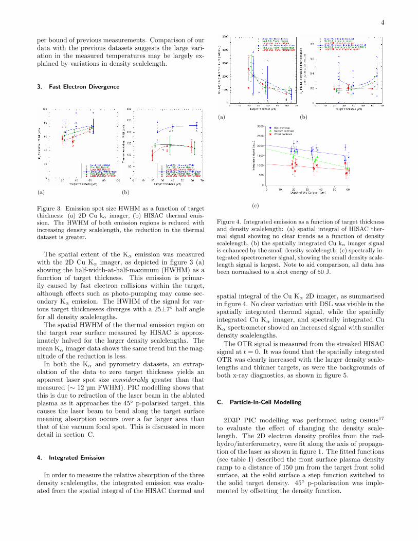
4

per bound of previous measurements. Comparison of ourdata with the previous datasets suggests the large vari-ation in the measured temperatures may be largely ex-plained by variations in density scalelength.

3. Fast Electron Divergence

(a) (b)

Figure 3. Emission spot size HWHM as a function of targetthickness: (a) 2D Cu kα imager, (b) HISAC thermal emis-sion. The HWHM of both emission regions is reduced withincreasing density scalelength, the reduction in the thermaldataset is greater.

The spatial extent of the Kα emission was measuredwith the 2D Cu Kα imager, as depicted in figure 3 (a)showing the half-width-at-half-maximum (HWHM) as afunction of target thickness. This emission is primar-ily caused by fast electron collisions within the target,although effects such as photo-pumping may cause sec-ondary Kα emission. The HWHM of the signal for var-ious target thicknesses diverges with a 25±7 half anglefor all density scalelengths.

The spatial HWHM of the thermal emission region onthe target rear surface measured by HISAC is approx-imately halved for the larger density scalelengths. Themean Kα imager data shows the same trend but the mag-nitude of the reduction is less.

In both the Kα and pyrometry datasets, an extrap-olation of the data to zero target thickness yields anapparent laser spot size considerably greater than thatmeasured (∼ 12 µm FWHM). PIC modelling shows thatthis is due to refraction of the laser beam in the ablatedplasma as it approaches the 45 p-polarised target, thiscauses the laser beam to bend along the target surfacemeaning absorption occurs over a far larger area thanthat of the vacuum focal spot. This is discussed in moredetail in section C.

4. Integrated Emission

In order to measure the relative absorption of the threedensity scalelengths, the integrated emission was evalu-ated from the spatial integral of the HISAC thermal and

(a) (b)

(c)

Figure 4. Integrated emission as a function of target thicknessand density scalelength: (a) spatial integral of HISAC ther-mal signal showing no clear trends as a function of densityscalelength, (b) the spatially integrated Cu kα imager signalis enhanced by the small density scalelength, (c) spectrally in-tegrated spectrometer signal, showing the small density scale-length signal is largest. Note to aid comparison, all data hasbeen normalised to a shot energy of 50 J.

spatial integral of the Cu Kα 2D imager, as summarisedin figure 4. No clear variation with DSL was visible in thespatially integrated thermal signal, while the spatiallyintegrated Cu Kα imager, and spectrally integrated CuKα spectrometer showed an increased signal with smallerdensity scalelengths.

The OTR signal is measured from the streaked HISACsignal at t = 0. It was found that the spatially integratedOTR was clearly increased with the larger density scale-lengths and thinner targets, as were the backgrounds ofboth x-ray diagnostics, as shown in figure 5.

C. Particle-In-Cell Modelling

2D3P PIC modelling was performed using osiris17

to evaluate the effect of changing the density scale-length. The 2D electron density profiles from the rad-hydro/interferometry, were fit along the axis of propaga-tion of the laser as shown in figure 1. The fitted functions(see table I) described the front surface plasma densityramp to a distance of 150 µm from the target front solidsurface, at the solid surface a step function switched tothe solid target density. 45 p-polarisation was imple-mented by offsetting the density function.

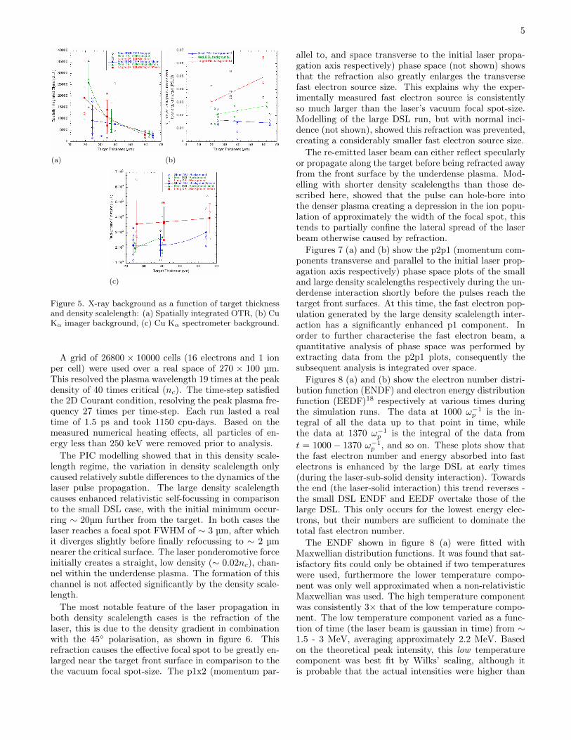
5

(a) (b)

(c)

Figure 5. X-ray background as a function of target thicknessand density scalelength: (a) Spatially integrated OTR, (b) CuKα imager background, (c) Cu Kα spectrometer background.

A grid of 26800 × 10000 cells (16 electrons and 1 ionper cell) were used over a real space of 270 × 100 µm.This resolved the plasma wavelength 19 times at the peakdensity of 40 times critical (nc). The time-step satisfiedthe 2D Courant condition, resolving the peak plasma fre-quency 27 times per time-step. Each run lasted a realtime of 1.5 ps and took 1150 cpu-days. Based on themeasured numerical heating effects, all particles of en-ergy less than 250 keV were removed prior to analysis.

The PIC modelling showed that in this density scale-length regime, the variation in density scalelength onlycaused relatively subtle differences to the dynamics of thelaser pulse propagation. The large density scalelengthcauses enhanced relativistic self-focussing in comparisonto the small DSL case, with the initial minimum occur-ring ∼ 20µm further from the target. In both cases thelaser reaches a focal spot FWHM of ∼ 3 µm, after whichit diverges slightly before finally refocussing to ∼ 2 µmnearer the critical surface. The laser ponderomotive forceinitially creates a straight, low density (∼ 0.02nc), chan-nel within the underdense plasma. The formation of thischannel is not affected significantly by the density scale-length.

The most notable feature of the laser propagation inboth density scalelength cases is the refraction of thelaser, this is due to the density gradient in combinationwith the 45 polarisation, as shown in figure 6. Thisrefraction causes the effective focal spot to be greatly en-larged near the target front surface in comparison to thethe vacuum focal spot-size. The p1x2 (momentum par-

allel to, and space transverse to the initial laser propa-gation axis respectively) phase space (not shown) showsthat the refraction also greatly enlarges the transversefast electron source size. This explains why the exper-imentally measured fast electron source is consistentlyso much larger than the laser’s vacuum focal spot-size.Modelling of the large DSL run, but with normal inci-dence (not shown), showed this refraction was prevented,creating a considerably smaller fast electron source size.

The re-emitted laser beam can either reflect specularlyor propagate along the target before being refracted awayfrom the front surface by the underdense plasma. Mod-elling with shorter density scalelengths than those de-scribed here, showed that the pulse can hole-bore intothe denser plasma creating a depression in the ion popu-lation of approximately the width of the focal spot, thistends to partially confine the lateral spread of the laserbeam otherwise caused by refraction.

Figures 7 (a) and (b) show the p2p1 (momentum com-ponents transverse and parallel to the initial laser prop-agation axis respectively) phase space plots of the smalland large density scalelengths respectively during the un-derdense interaction shortly before the pulses reach thetarget front surfaces. At this time, the fast electron pop-ulation generated by the large density scalelength inter-action has a significantly enhanced p1 component. Inorder to further characterise the fast electron beam, aquantitative analysis of phase space was performed byextracting data from the p2p1 plots, consequently thesubsequent analysis is integrated over space.

Figures 8 (a) and (b) show the electron number distri-bution function (ENDF) and electron energy distributionfunction (EEDF)18 respectively at various times duringthe simulation runs. The data at 1000 ω−1

p is the in-tegral of all the data up to that point in time, whilethe data at 1370 ω−1

p is the integral of the data from

t = 1000 − 1370 ω−1p , and so on. These plots show that

the fast electron number and energy absorbed into fastelectrons is enhanced by the large DSL at early times(during the laser-sub-solid density interaction). Towardsthe end (the laser-solid interaction) this trend reverses -the small DSL ENDF and EEDF overtake those of thelarge DSL. This only occurs for the lowest energy elec-trons, but their numbers are sufficient to dominate thetotal fast electron number.

The ENDF shown in figure 8 (a) were fitted withMaxwellian distribution functions. It was found that sat-isfactory fits could only be obtained if two temperatureswere used, furthermore the lower temperature compo-nent was only well approximated when a non-relativisticMaxwellian was used. The high temperature componentwas consistently 3× that of the low temperature compo-nent. The low temperature component varied as a func-tion of time (the laser beam is gaussian in time) from ∼1.5 - 3 MeV, averaging approximately 2.2 MeV. Basedon the theoretical peak intensity, this low temperaturecomponent was best fit by Wilks’ scaling, although itis probable that the actual intensities were higher than

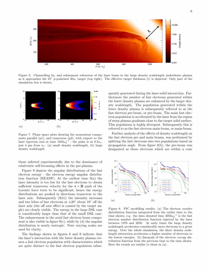
6

t

Wednesday, 16 March 2011

Figure 6. Channelling by, and subsequent refraction of the laser beam in the large density scalelength underdense plasmaas it approaches the 45 p-polarised 40nc target (top right). The effective target thickness (t) is depicted. Only part of thesimulation box is shown.

(a) (b)

Figure 7. Phase space plots showing the momentum compo-nents parallel (p1), and transverse (p2), with respect to thelaser injection axis at time 1035ω−1

p - the pulse is at 0.5nc,just 4 µm from nc: (a) small density scalelength, (b) largedensity scalelength.

those inferred experimentally due to the dominance ofrelativistic self-focussing effects in the pre-plasma.

Figure 9 depicts the angular distributions of the fastelectron energy - the electron energy angular distribu-tion function (EEADF). At the earliest time 9(a) thelaser intensity is too low for the fast electrons to obtainsufficient transverse velocity for the v ×B push of theLorentz force term to be significant, hence the energydistributions are peaked in directions transverse to thelaser axis. Subsequently (9(b)) the intensity increasesand two lobes of fast electrons at ±20 about 10 off thelaser axis (the off axis effect is caused by the target an-gle) are clearly visible. The energy in the large DSL caseis considerably larger than that of the small DSL case.The enhancement in the axial fast electron beam compo-nent is also visible in figure 9(c), while by (d) the angulardistribution is nearly isotropic. Note varying scales areused for clarity.

The findings shown in figures 8 and 9 indicate thatthe laser’s interaction with the lower density plasma cre-ates a fast electron population with characteristics whichare quite distinct to the fast electron population subse-

quently generated during the laser-solid interaction. Fur-thermore the number of fast electrons generated withinthe lower density plasma are enhanced by the larger den-sity scalelength. The population generated within thelower density plasma is subsequently referred to as thefast electron pre-beam, or pre-beam. The main fast elec-tron population is accelerated by the laser from the regionof steep plasma gradients close to the target solid surface.This population is highly divergent. Subsequently this isreferred to as the fast electron main-beam, or main-beam.

Further analysis of the effects of density scalelength onthe fast electron pre and main beams, was performed bysplitting the fast electrons into two populations based onpropagation angle. From figure 9(b), the pre-beam wasdesignated as those electrons which are within a cone

(a)

105

107

109

1011

1013

1015

1 10 100

low and high_c 17run endf

Small DSL 1000ωp-1

Small DSL 1370ωp-1

Small DSL 2050ωp-1

Large DSL 1000ωp-1

Large DSL 1370ωp-1

Large DSL 2050ωp-1

Elec

tron

num

ber/M

eV

Electron energy (MeV)

(b)

105

107

109

1011

1013

1 10 100

low and high_c 17run eedf

Small DSL 1000ωp-1

Small DSL 1370ωp-1

Small DSL 2050ωp-1

Large DSL 1000ωp-1

Large DSL 1370ωp-1

Large DSL 2050ωp-1

Elec

tron

ener

gy (M

eV/M

eV)

Electron energy (MeV)

Figure 8. PIC modelling results: (a) The electron numberdistribution function integrated from the earlier time to thetime shown, e.g. the data denoted time 2050ω−1

p is the fastelectron number distribution function injected by the laserbetween 1370 and 2050. At early times the large densityscalelength accelerates considerably more electrons to a givenenergy. Over the whole simulation, the short density scale-length interaction accelerates a higher number of electrons tothe lowest energies. (b) Integrals of the electron energy dis-tribution function from the previous time to the time shown.Here the trends are similar to those in (a).

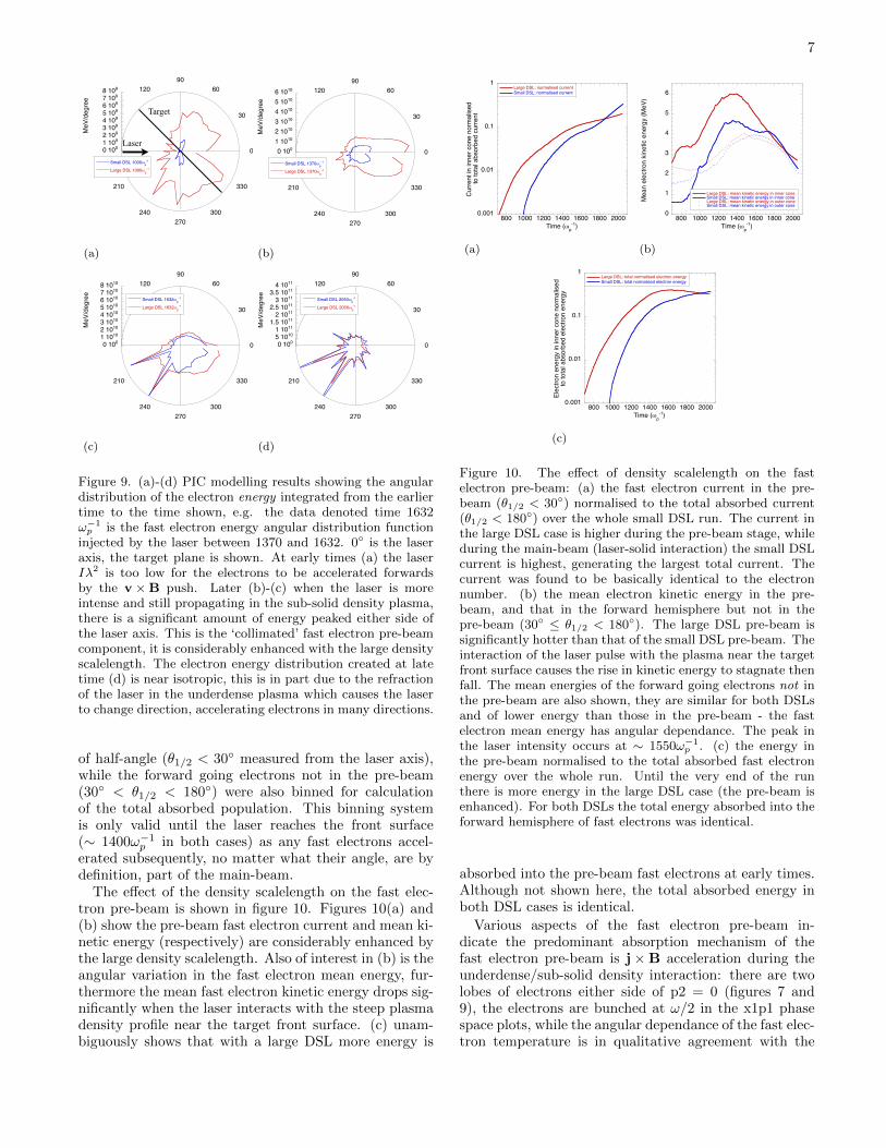
7

(a)

Laser

Target

0 1001 1092 1093 1094 1095 1096 1097 1098 109

0

30

6090

120

210

240270

300

330

17runs eeadf@t=1000

Small DSL 1000!p-1

Large DSL 1000!p-1

MeV

/deg

ree

Thursday, 10 March 2011

(b)

0 1001 10102 10103 10104 10105 10106 1010

0

30

6090

120

210

240270

300

330

17runs eeadf@t=1370

Small DSL 1370ωp-1

Large DSL 1370ωp-1

MeV

/deg

ree

(c)

0 1001 10102 10103 10104 10105 10106 10107 10108 1010

0

30

6090

120

210

240270

300

330

17runs eeadf@t=1632

Small DSL 1632ωp-1

Large DSL 1632ωp-1

MeV

/deg

ree

(d)

0 1005 10101 1011

1.5 10112 1011

2.5 10113 1011

3.5 10114 1011

0

30

6090

120

210

240270

300

330

17runs eeadf@t=2050

Small DSL 2050ωp-1

Large DSL 2050ωp-1

MeV

/deg

ree

Figure 9. (a)-(d) PIC modelling results showing the angulardistribution of the electron energy integrated from the earliertime to the time shown, e.g. the data denoted time 1632ω−1p is the fast electron energy angular distribution function

injected by the laser between 1370 and 1632. 0 is the laseraxis, the target plane is shown. At early times (a) the laserIλ2 is too low for the electrons to be accelerated forwardsby the v ×B push. Later (b)-(c) when the laser is moreintense and still propagating in the sub-solid density plasma,there is a significant amount of energy peaked either side ofthe laser axis. This is the ‘collimated’ fast electron pre-beamcomponent, it is considerably enhanced with the large densityscalelength. The electron energy distribution created at latetime (d) is near isotropic, this is in part due to the refractionof the laser in the underdense plasma which causes the laserto change direction, accelerating electrons in many directions.

of half-angle (θ1/2 < 30 measured from the laser axis),while the forward going electrons not in the pre-beam(30 < θ1/2 < 180) were also binned for calculationof the total absorbed population. This binning systemis only valid until the laser reaches the front surface(∼ 1400ω−1

p in both cases) as any fast electrons accel-erated subsequently, no matter what their angle, are bydefinition, part of the main-beam.

The effect of the density scalelength on the fast elec-tron pre-beam is shown in figure 10. Figures 10(a) and(b) show the pre-beam fast electron current and mean ki-netic energy (respectively) are considerably enhanced bythe large density scalelength. Also of interest in (b) is theangular variation in the fast electron mean energy, fur-thermore the mean fast electron kinetic energy drops sig-nificantly when the laser interacts with the steep plasmadensity profile near the target front surface. (c) unam-biguously shows that with a large DSL more energy is

(a)

0.001

0.01

0.1

1

800 1000 1200 1400 1600 1800 2000

current within a cone of half angle 30 degrees relative to total current over 180

degrees (i.e those which go into the target) in small dsl case

Large DSL: normalised currentSmall DSL: normalised current

Cur

rent

in in

ner c

one

norm

alis

ed

to to

tal a

bsor

bed

curre

nt

Time (ωp-1)

(b)

0

1

2

3

4

5

6

800 1000 1200 1400 1600 1800 2000

mean e kinetic energy within a cone of half angle 30 degrees and mean e kintic energy 180

degrees but not in inner cone

Large DSL: mean kinetic energy in inner coneSmall DSL: mean kinetic energy in inner coneLarge DSL: mean kinetic energy in outer coneSmall DSL: mean kinetic energy in outer cone

Mea

n el

ectro

n ki

netic

ene

rgy

(MeV

)

Time (ωp-1)

(c)

0.001

0.01

0.1

1

800 1000 1200 1400 1600 1800 2000

e energy within a cone of half angle 30 degrees relative to total e energy over 180

degrees (i.e those which go into the target)

Large DSL: total normalised electron energySmall DSL: total normalised electron energy

Elec

tron

ener

gy in

inne

r con

e no

rmal

ised

to

tota

l abs

orbe

d el

ectro

n en

ergy

Time (ωp-1)

Figure 10. The effect of density scalelength on the fastelectron pre-beam: (a) the fast electron current in the pre-beam (θ1/2 < 30) normalised to the total absorbed current(θ1/2 < 180) over the whole small DSL run. The current inthe large DSL case is higher during the pre-beam stage, whileduring the main-beam (laser-solid interaction) the small DSLcurrent is highest, generating the largest total current. Thecurrent was found to be basically identical to the electronnumber. (b) the mean electron kinetic energy in the pre-beam, and that in the forward hemisphere but not in thepre-beam (30 ≤ θ1/2 < 180). The large DSL pre-beam issignificantly hotter than that of the small DSL pre-beam. Theinteraction of the laser pulse with the plasma near the targetfront surface causes the rise in kinetic energy to stagnate thenfall. The mean energies of the forward going electrons not inthe pre-beam are also shown, they are similar for both DSLsand of lower energy than those in the pre-beam - the fastelectron mean energy has angular dependance. The peak inthe laser intensity occurs at ∼ 1550ω−1

p . (c) the energy inthe pre-beam normalised to the total absorbed fast electronenergy over the whole run. Until the very end of the runthere is more energy in the large DSL case (the pre-beam isenhanced). For both DSLs the total energy absorbed into theforward hemisphere of fast electrons was identical.

absorbed into the pre-beam fast electrons at early times.Although not shown here, the total absorbed energy inboth DSL cases is identical.

Various aspects of the fast electron pre-beam in-dicate the predominant absorption mechanism of thefast electron pre-beam is j×B acceleration during theunderdense/sub-solid density interaction: there are twolobes of electrons either side of p2 = 0 (figures 7 and9), the electrons are bunched at ω/2 in the x1p1 phasespace plots, while the angular dependance of the fast elec-tron temperature is in qualitative agreement with the

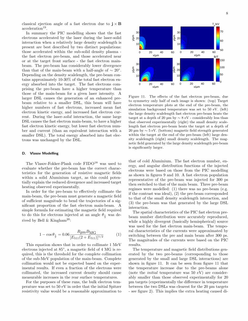
8

classical ejection angle of a fast electron due to j×Bacceleration19.

In summary the PIC modelling shows that the fastelectrons accelerated by the laser during the laser-solidinteraction when a relatively large density scalelength ispresent are best described by two distinct populations:those accelerated within the sub-solid density plasma -the fast electron pre-beam, and those accelerated nearor at the target front surface - the fast electron main-beam. The pre-beam has considerably lower divergencethan that of the main-beam with a half-angle of ∼ 20.Depending on the density scalelength, the pre-beam con-tains approximately 10-30% of the total fast electron en-ergy absorbed into the target. The fast electrons com-prising the pre-beam have a higher temperature thanthose of the main-beam for a given laser intensity. Alarger DSL causes the generation of an enhanced pre-beam relative to a smaller DSL, this beam will havehigher numbers of fast electrons, increased mean fastelectron kinetic energy, and increased fast electron cur-rent. During the laser-solid interaction, the same largeDSL causes the fast electron main-beam, to have a higherfast electron kinetic energy, but lower fast electron num-ber and current (than an equivalent interaction with asmaller DSL). The total energy absorbed into fast elec-trons was unchanged by the DSL.

D. Vlasov Modelling

The Vlasov-Fokker-Plank code FIDO18 was used toevaluate whether the pre-beam has the correct charac-teristics for the generation of resistive magnetic fieldswithin a solid Aluminium target, as this could poten-tially explain the reduced divergence and increased targetheating observed experimentally.

In order for the pre-beam to effectively collimate themain-beam, the pre-beam must generate a magnetic fieldof sufficient magnitude to bend the trajectories of a sig-nificant proportion of the fast electron main-beam. Asimple formula for estimating the magnetic field requiredto do this for electrons injected at an angle θ 1

2was de-

rived by Bell & Kingham20:

1 − cos θ 12

= 0.06RµmBMG

[E511(2 + E511)]1/2(1)

This equation shows that in order to collimate 1 MeVelectrons injected at 85, a magnetic field of 4 MG is re-quired, this is the threshold for the complete collimationof the sub-MeV population of the main-beam. Completecollimation would not be expected based on the exper-imental results. If even a fraction of the electrons werecollimated, the increased current density should causemeasurable increases in the rear surface temperatures.

For the purposes of these runs, the bulk electron tem-perature was set to 50 eV in order that the initial Spitzerresistivity value would be a reasonable approximation to

x/µm

y/µm

0 20 40 60

10

20

30

x/µm

y/µm

0 20 40 60

10

20

30

50

60

70

x/µm

y/µm

0 20 40 60

10

20

30

x/µm

y/µm

0 20 40 60

10

20

30

0

50

100

150

Te/eV

B/T

Figure 11. The effects of the fast electron pre-beam, dueto symmetry only half of each image is shown: (top) Targetelectron temperature plots at the end of the pre-beam, thesimulation background temperature was set to 50 eV. (left)the large density scalelength fast electron pre-beam heats thetarget at a depth of 20 µm by ∼ 8 eV - considerably less thanthat observed experimentally (right) the small density scale-length fast electron pre-beam heats the target at a depth of20 µm by ∼ 5 eV. (bottom) magnetic field strength generatedwithin the target at the end of the pre-beam (left) large den-sity scalelength (right) small density scalelength. The mag-netic field generated by the large density scalelength pre-beamis significantly larger.

that of cold Aluminium. The fast electron number, en-ergy, and angular distribution functions of the injectedelectrons were based on those from the PIC modellingas shown in figures 9 and 10. A fast electron populationrepresentative of the pre-beam was injected for 300 psthen switched to that of the main beam. Three pre-beamregimes were modelled: (1) there was no pre-beam (e.g.if the contrast was ideal), (2) the pre-beam correspondedto that of the small density scalelength interaction, and(3) the pre-beam was that generated by the large DSLinteraction.

The spatial characteristics of the PIC fast electron pre-beam number distribution were accurately reproduced,while a highly divergent (basically hemispherical) sourcewas used for the fast electron main-beam. The tempo-ral characteristics of the currents were approximated byswitching between the pre and main beam after 300 ps.The magnitudes of the currents were based on the PICresults.

The temperature and magnetic field distributions gen-erated by the two pre-beams (corresponding to thosegenerated by the small and large DSL interactions) areshown in figure 11. It can be seen from figure 11 thatthe temperature increase due to the pre-beams alone(note the initial temperature was 50 eV) are consider-ably smaller than those observed experimentally for 20µm targets (experimentally the difference in temperaturebetween the two DSLs was clearest for the 20 µm targets- see figure 2). This implies the extra heating caused di-

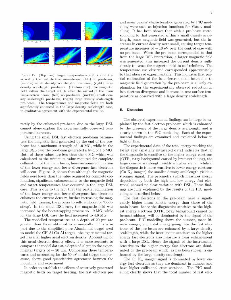
9

x/µm

y/µm

0 10 20 30 40 50 60

5

10

15

20

25

30

35 63eV

79eV

100eV

126eV

200eV

158eV

x/µm

y/µm

0 10 20 30 40 50 60

5

10

15

20

25

30

35

79eV

100eV

158eV

126eV

63eV

200eV

x/µm

y/µm

0 10 20 30 40 50 60

5

10

15

20

25

30

35 126eV

158eV

200eV

251eV

316eV

100eV63eV79eV

x/µm

y/µm

0 10 20 30 40 50 60

5

10

15

20

25

30

35

100T

631T

40T

16T

63T

x/µm

y/µm

0 10 20 30 40 50 60

5

10

15

20

25

30

35

631T

16T

40T

100T158T

x/µm

y/µm

0 10 20 30 40 50 60

5

10

15

20

25

30

35

16T40T

251T100T

631T

Figure 12. (Top row) Target temperatures 400 fs after thearrival of the fast electron main-beam: (left) no pre-beam,(middle) small density scalelength pre-beam, (right) largedensity scalelength pre-beam. (Bottom row) The magneticfield within the target 400 fs after the arrival of the mainfast-electron beam: (left) no pre-beam, (middle) small den-sity scalelength pre-beam, (right) large density scalelengthpre-beam. The temperatures and magnetic fields are bothsignificantly enhanced in the large density scalelength case,in qualitative agreement with the experimental results.

rectly by the enhanced pre-beam due to the large DSLcannot alone explain the experimentally observed tem-perature increases.

Using the small DSL fast electron pre-beam parame-ters the magnetic field generated by the end of the pre-beam has a maximum strength of 1.0 MG, while in thelarge DSL case the pre-beam generated a field of 1.6 MG.Both of these values are less than the 4 MG which wascalculated as the minimum value required for completecollimation of the main beam, however some collimationof the lower energy and lower divergence fast electronswill occur. Figure 12, shows that although the magneticfields were lower than the value required for complete col-limation, significant enhancements to the magnetic fieldand target temperatures have occurred in the large DSLcase. This is due to the fact that the partial collimationof the lower energy and lower divergence fast electronsenhances the current density, further increasing the mag-netic field, causing the process to self-reinforce, or ‘boot-strap’. In the small DSL case, the magnetic field wasincreased by the bootstrapping process to 1.9 MG, whilefor the large DSL case the field increased to 4.6 MG.

The modelled temperatures at a depth of 20 µm aregreater than those obtained experimentally. This is inpart due to the simplified pure Aluminium target usedto model the CH-Al-Cu-Al target - the experimental tar-get has a far higher areal electron density. Accounting forthis areal electron density effect, it is more accurate tocompare the model data at a depth of 40 µm to the exper-imental targets of ∼ 20 µm. Comparing these tempera-tures and accounting for the 50 eV initial target temper-ature, shows good quantitative agreement between themodelling and experiment.

In order to establish the effects of resistively generatedmagnetic fields on target heating, the fast electron pre

and main beams’ characteristics generated by PIC mod-elling were used as injection functions for Vlasov mod-elling. It has been shown that with a pre-beam corre-sponding to that generated within a small density scale-length, some magnetic field was generated, but the in-creases in current density were small, causing target tem-perature increases of ∼ 10 eV over the control case withno pre-beam. When the pre-beam corresponded to thatfrom the large DSL interaction, a larger magnetic fieldwas generated, this increased the current density suffi-ciently to cause the magnetic field to self-reinforce. Thetemperature rise observed corresponded approximatelyto that observed experimentally. This indicates that par-tial collimation of the fast electron main-beam due tomagnetic field generation by the pre-beam is a likely ex-planation for the experimentally observed reduction infast electron divergence and increase in rear surface tem-perature as observed with a large density scalelength.

E. Discussion

The observed experimental findings can in large be ex-plained by the fast electron pre-beam which is enhancedby the presence of the large density scalelength and isclearly shown in the PIC modelling. Each of the exper-imental findings are examined and explained below inlight of this.

The experimental data of the total energy reaching thetarget rear (spatially integrated data) indicates that, ifthe diagnostic is sensitive to the higher energy electrons(OTR, x-ray background caused by bremsstrahlung), thelarge density scalelength yields a higher signal, while ifthe diagnostic is more sensitive to lower energy electrons(Cu Kα imager) the smaller density scalelength yields astronger signal. The pyrometry (which measures energydeposition by both the high and low energy fast elec-trons) showed no clear variation with DSL. These find-ings are fully explained by the results of the PIC mod-elling as described below.

The fast electrons in the pre-beam have a signifi-cantly higher mean kinetic energy than those of themain beam, hence the diagnostics sensitive to the high-est energy electrons (OTR, x-ray background caused bybremsstrahlung) will be dominated by the signal of thepre-beam. PIC modelling shows the number, mean ki-netic energy, and total energy going into the fast elec-trons of the pre-beam are enhanced by a large densityscalelength, while the instruments sensitive to the higherenergy fast electrons also measure a clear enhancementwith a large DSL. Hence the signals of the instrumentssensitive to the higher energy fast electrons are domi-nated by the pre-beam which, as has been shown, is en-hanced by the large density scalelength.

The Cu Kα imager signal is dominated by lower en-ergy fast electrons as they are dominant in number andhave higher collisional cross sections. The PIC mod-elling clearly shows that the total number of fast elec-

10

trons absorbed over the whole interaction is significantlyenhanced with a small density scalelength, but this domi-nance is only due to the lowest energy fast electrons. Thisis in agreement with the spatially integrated Cu Kα im-ager results - explaining the experimental observations.

Finally the pyrometry observes no clear change in thetotal energy reaching the target rear as a function of den-sity scalelength. This instrument measures energy depo-sition at the target rear by both the high and low energyfast electrons via Ohmic and collisional heating. The PICmodelling showed that the total energy absorbed was in-variant with density scalelength, thereby explaining thepyrometric experimental observations.

The rear surface temperatures measured by the Cu Kα

spectroscopy and pyrometry were of the same order, how-ever the spectroscopy did not show the factor of four tem-perature increase for the thinner targets and large densityscalelength. This was ascribed to the lack of sensitivityof the spectrometer, similar observations have been madeover numerous expeirments.

All of the diagnostics found the spot-size HWHMcaused by the electron transport within the target wasreduced with a large density scalelength. The reductionin the spot-size HWHM was considerably larger in thecases of the thermal and OTR than that of the Cu Kα im-ager. The reduction is attributed to the more collimatednature of, and increased current in, the fast electron pre-beam generated by the sub-solid density interaction inthe large DSL case. The exact mechanism by which thisreduction in spot size occurs is discussed in more detailbelow.

Vlasov modelling showed that the pre-beam only in-creased the target temperature by ∼ 8 eV in the largeDSL case - insufficient to explain the pyrometrically ob-served increases in rear surface temperature.

It was found that the fast electron pre-beam gener-ated by the small density scalelength could generate somemagnetic field but it was insufficient to cause significantcollimation of the main-beam, and the observed temper-atures rises were small. The large density scalelengthinteraction was sufficient to cause partial collimation ofthe subsequent fast electron main-beam and resultant in-creases in rear surface temperatures were of the order of60 eV - similar to those observed experimentally.

Fast ignition inertial confinement fusion requires theignition electron beam to have a mean energy of ∼ 1MeV. The enhancement in forward energy flux whichhas been demonstrated with the large density scalelengthpre-plasma is principally due to the creation of a pre-beam of fast electrons of increased number and mean ki-netic energy but reduced divergence (in comparison tothose fast electrons generated near the solid surface).The fast electron pre-beam does not have the correctcharacteristics for a fast ignition ICF driver as the meanfast electron kinetic energy is too high and there are in-sufficient electrons within the pre-plasma, however it maypossess useful characteristics with regards to the creationof a magnetic field structure which could collimate (or

at least reduce the divergence of) the highly divergent,colder electrons accelerated at the solid-surface (be thatan embedded cone or surface of a compressed ICF cap-sule).B ≈ ηjt/R approximates the resistively generated

magnetic field by a fast electron beam propagating in asolid21, where B is the magnetic field, j the current den-sity, t the laser duration and R the electron beam radius.This is now applied in a fast ignition relevant scenario.Assuming η = 1.6 × 10−8Ω −m (Spitzer resistivity for 1keV D-T ), a fast electron beam radius of 10 µm, a laserpulse duration of 1 ps, and a mean fast electron energy of5 MeV (the temperature of the fast electron pre-beam),the total energy in the electron beam would be requiredto be ∼ 500 J in order to create a 400 T magnetic fieldwhich extends 200 µm into the solid, compressed D-T.Within this field the 1 MeV electrons will have a Larmorradius of the order of the magnetic field radius, and hencewill be confined by the magnetic field ‘structure’. Thisshows that in principle it is possible to use the initialhigh energy population of electrons to draw a sufficientresistive return current within a fast ignition relevant sce-nario in order to generate a magnetic field suitable for thecollimation of the bulk electron population.

This scheme is similar to the artificial collimation tech-nique proposed by Robinson et al21, however it has theadvantage that the initial population is of higher tem-perature and importantly, is more collimated than thatof the bulk electron population, hence it may be possibleto set up a magnetic field which extends deep into thecompressed DT core, guiding the fast electrons withinthe DT until they deposit their energy.

F. Summary

In conclusion, when a sufficiently large density scale-length exists (see table I), the fast electron beam result-ing from the laser-solid interaction is best described bytwo distinct populations: those accelerated within thesub-solid density plasma - the fast electron pre-beam,and those accelerated near or at the target front surface- the fast electron main-beam.

The fast electron pre-beam has considerably lower di-vergence than that of the main-beam with a half-angleof ∼ 20. Depending on the density scalelength, the pre-beam contains approximately 10-30% of the total fastelectron energy absorbed into the target. The fast elec-trons comprising the pre-beam have a higher temperaturethan those of the main-beam for a given laser intensity.

A larger DSL causes the generation of an enhancedfast electron pre-beam during the sub-solid density in-teraction, this beam will have higher numbers of fastelectrons, increased mean kinetic energy, and increasedcurrent. The same large DSL causes the main-beam gen-erated at or near the solid surface, to have a higher fastelectron kinetic energy, but lower fast electron numberand current. The total energy absorbed into fast elec-

11

trons was unchanged by the DSL.There is strong evidence that with a larger density

scalelength, the fast electrons heat a smaller cross sec-tional area of the target, causing the thinnest targetsto reach significantly higher rear surface temperatures.Based on the modelling performed it is most likely thisis due to the enhanced fast electron pre-beam associatedwith the large density scalelength interaction. This gen-erates a magnetic field within the target of sufficient mag-nitude to partially collimate the subsequent more diver-gent fast electron main-beam.

The fast electron pre-beam may have suitable proper-ties to generate a magnetic field within the compressedDT core of a fast ignition ICF capsule. This magneticfield structure would act to collimate the subsequent pop-ulation of highly divergent electrons accelerated from thesolid surface. Simple calculations show this is energeti-cally feasible requiring less than 1% of the ignition laserenergy. More detailed work is required to accurately as-sess the viability of such a scheme.

This work has two main findings in the context of fastignition. Firstly, if it is not possible to generate a mag-netic field in the manner described above, higher con-trasts are advantageous for fast ignition as they increasethe fast electron current and reduce the fast electron’smean kinetic energy. Secondly, the hole boring phase ofcone-less fast ignition inertial confinement fusion may beused to generate a fast electron pre-beam with suitablecharacteristics for the divergence reduction of the fastelectron main-beam generated by the laser-solid interac-tion.

REFERENCES

1E. L. Clark et al., Phys. Rev. Lett. 84, 670 (2000).

2R. A. Snavely et al., Phys. Rev. Lett. 85, 2945 (2000).3A. Maksimchuk et al., Phys. Rev. Lett. 84, 4108 (2000).4D. Hoarty et al., High Energy Density Phys. 3, 115 (2007).5M. Tabak et al., Phys. Plamas 1, 1626 (1994), part 2.6A. J. Kemp, Y. Sentoku, and M. Tabak, Phys. Rev. E 79, 066406(2009).

7S. C. Wilks and W. L. Kruer, IEEE J. Quantum Electronics 33(1997).

8P.-H. Maire, J. Breil, and S. Galera, International Journal forNumerical Methods in Fluids 56, 1161 (2008).

9A. L. Meadowcroft, C. D. Bentley, and E. N. Stott, Review ofScientific Instruments 79, 113102 (2008).

10H.-K. Chung et al., High Energy Density Physics 1, 3 (2005),ISSN 1574-1818.

11R. Kodama, K. Okada, and Y. Kato, Review of Scientific Instru-ments 70, 625 (1999).

12N. C. Woolsey et al., Phys. Rev. E 57, 4650 (1998).13A. R. Bell et al., Plasma Phys. & Controlled Fusion 39, 653

(1997).14J. J. Santos et al., Phys. Rev. Lett. 89 (2002), fast elec-

tron transport in ultraintense laser pulse interaction with solidtargets by rear-side self-radiation diagnostics 10.1103/Phys-RevLett.89.025001.

15J. Zheng et al., Phys. Plamas 10, 2994 (2003).16S. D. Baton et al., Phys. Rev. Lett. 91, 105001 (2003).17R. Fonseca et al., in P. Sloot et al., editors, Computational Sci-

ence — ICCS 2002, volume 2331 of Lecture Notes in ComputerScience, pages 342–351, Springer Berlin / Heidelberg (2002).

18M. Sherlock, Phys. Plamas 16, 103101 (2009).19R. B. Stephens et al., Phys. Rev. E 69, 066414 (2004), copy-

right (C) 2008 The American Physical Society Please report anyproblems to prola@aps.org PRE.

20A. R. Bell and R. J. Kingham, Phys. Rev. Lett. 91, 035003(2003), copyright (C) 2008 The American Physical Society Pleasereport any problems to prola@aps.org PRL.

21A. P. L. Robinson, M. Sherlock, and P. A. Norreys, Phys. Rev.Lett. 100, 025002 (2008).

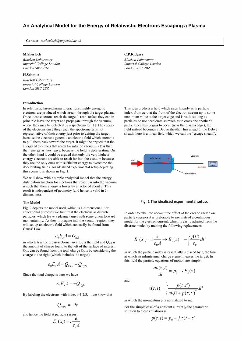
An Analytical Model for the Energy of Relativistic Electrons Escaping a Plasma

M.Sherlock Blackett Laboratory Imperial College London London SW7 2BZ

H.Schmitz Blackett Laboratory Imperial College London London SW7 2BZ

C.P.Ridgers Blackett Laboratory Imperial College London London SW7 2BZ

Introduction In relativistic laser-plasma interactions, highly energetic electrons are produced which stream through the target plasma. Once these electrons reach the target’s rear surface they can in principle leave the target and propagate through the vacuum, where they may be detected by a spectrometer [1]. The energy of the electrons once they reach the spectrometer is not representative of their energy just prior to exiting the target, because the electrons generate an electric field which attempts to pull them back toward the target. It might be argued that the energy of electrons that reach far into the vacuum is less than their energy as they leave, because the field is decelerating. On the other hand it could be argued that only the very highest energy electrons are able to reach far into the vacuum because they are the only ones with sufficient energy to overcome the decelerating fields. An idealised experimental setup depicting this scenario is shown in Fig. 1.

We will show with a simple analytical model that the energy distribution function for electrons that reach far into the vacuum is such that their energy is lower by a factor of about 2. This result is independent of geometry (and hence is valid in 3-dimensions).

The Model Fig. 2 depicts the model used, which is 1-dimensional. For educational purposes we first treat the electrons as discrete particles, which leave a plasma target with some given forward momentum p0. As they propagate into the vacuum region, they will set up an electric field which can easily be found from Gauss’ Law:

in which A is the cross-sectional area, Ex is the field and Qleft is the amount of charge found to the left of the surface of interest. Qleft can be found from the total charge Qtotal by considering the charge to the right (which includes the target):

Since the total charge is zero we have

By labeling the electrons with index i=1,2,3…, we know that

and hence the field at particle i is just

This idea predicts a field which rises linearly with particle index, from zero at the front of the electron stream up to some maximum value at the target edge and is valid so long as particles do not decelerate so much as to cross one another’s paths. Once this begins to occur (near the plasma edge), the field instead becomes a Debye sheath. Thus ahead of the Debye sheath there is a linear field which we call the “escape sheath”.

In order to take into account the effect of the escape sheath on particle energies it is preferable to use instead a continuous model for the electron current, which is easily adapted from the discrete model by making the following replacement:

in which the particle index is essentially replaced by τ, the time at which an infinitesimal charge element leaves the target. In this field the particle equations of motion are simply:

and

in which the momentum p is normalized to mc.

For the simple case of a constant current j0 the parametric solution to these equations is:

Contact m.sherlock@imperial.ac.uk

0 х leftЕ A Q

0 х total rightЕ A Q Q

0 х rightЕ A Q

rightQ ie

0

( )х i

eЕ x i

A

0 00

( ')( ) ( ) 'х i х

e j tЕ x i Е dt

A

0( , ) ( )х

dp tp eЕ

dt

20

( , ')( , ) '1 ( , ')

t p tx t dt

m p t

0 0( , ) ( )p t p j t

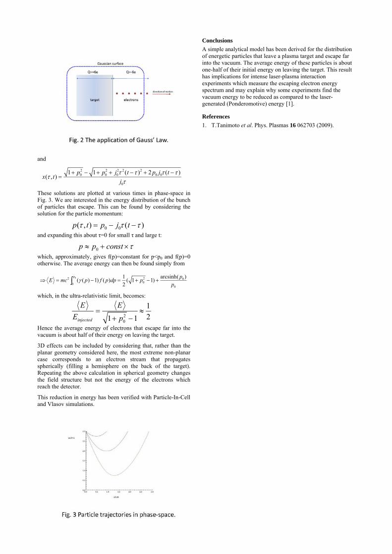
and

These solutions are plotted at various times in phase-space in Fig. 3. We are interested in the energy distribution of the bunch of particles that escape. This can be found by considering the solution for the particle momentum:

and expanding this about τ=0 for small τ and large t:

which, approximately, gives f(p)=constant for p<p0 and f(p)=0 otherwise. The average energy can then be found simply from

which, in the ultra-relativistic limit, becomes:

Hence the average energy of electrons that escape far into the vacuum is about half of their energy on leaving the target.

3D effects can be included by considering that, rather than the planar geometry considered here, the most extreme non-planar case corresponds to an electron stream that propagates spherically (filling a hemisphere on the back of the target). Repeating the above calculation in spherical geometry changes the field structure but not the energy of the electrons which reach the detector.

This reduction in energy has been verified with Particle-In-Cell and Vlasov simulations.

Conclusions A simple analytical model has been derived for the distribution of energetic particles that leave a plasma target and escape far into the vacuum. The average energy of these particles is about one-half of their initial energy on leaving the target. This result has implications for intense laser-plasma interaction experiments which measure the escaping electron energy spectrum and may explain why some experiments find the vacuum energy to be reduced as compared to the laser-generated (Ponderomotive) energy [1].

References 1. T.Tanimoto et al. Phys. Plasmas 16 062703 (2009).

2 2 2 2 20 0 0 0 0

0

1 1 ( ) 2 ( )( , )

p p j t p j tx t

j

0 0( , ) ( )p t p j t

0p p const

02 2 000

0

1 arcsinh( )( ( ) 1) ( ) ( 1 1)2

p pE mc p f p dp p

p

20

121 1injected

E E

E p

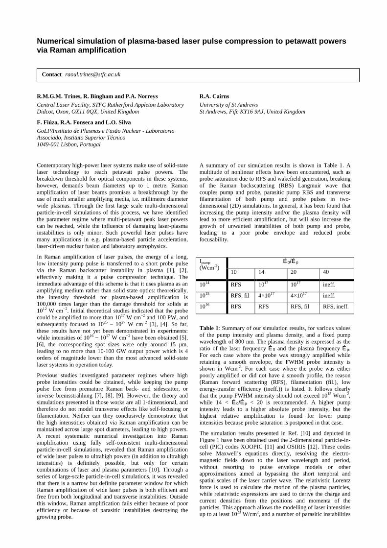
R.M.G.M. Trines, R. Bingham and P.A. Norreys

Central Laser Facility, STFC Rutherford Appleton Laboratory Didcot, Oxon, OX11 0QX, United Kingdom

F. Fiúza, R.A. Fonseca and L.O. Silva

GoLP/Instituto de Plasmas e Fusão Nuclear - Laboratorio Associado, Instituto Superior Técnico 1049-001 Lisbon, Portugal

R.A. Cairns

University of St Andrews St Andrews, Fife KY16 9AJ, United Kingdom

Contemporary high-power laser systems make use of solid-state laser technology to reach petawatt pulse powers. The breakdown threshold for optical components in these systems, however, demands beam diameters up to 1 metre. Raman amplification of laser beams promises a breakthrough by the use of much smaller amplifying media, i.e. millimetre diameter wide plasmas. Through the first large scale multi-dimensional particle-in-cell simulations of this process, we have identified the parameter regime where multi-petawatt peak laser powers can be reached, while the influence of damaging laser-plasma instabilities is only minor. Such powerful laser pulses have many applications in e.g. plasma-based particle acceleration, laser-driven nuclear fusion and laboratory astrophysics.

In Raman amplification of laser pulses, the energy of a long, low intensity pump pulse is transferred to a short probe pulse via the Raman backscatter instability in plasma [1], [2], effectively making it a pulse compression technique. The immediate advantage of this scheme is that it uses plasma as an amplifying medium rather than solid state optics: theoretically, the intensity threshold for plasma-based amplification is 100,000 times larger than the damage threshold for solids at 1012 W cm−2. Initial theoretical studies indicated that the probe could be amplified to more than 1017 W cm−2 and 100 PW, and subsequently focused to 1025 – 1027 W cm−2 [3], [4]. So far, these results have not yet been demonstrated in experiments: while intensities of 1016 − 1017 W cm−2 have been obtained [5], [6], the corresponding spot sizes were only around 15 µm, leading to no more than 10-100 GW output power which is 4 orders of magnitude lower than the most advanced solid-state laser systems in operation today.

Previous studies investigated parameter regimes where high probe intensities could be obtained, while keeping the pump pulse free from premature Raman back- and sidescatter, or inverse bremsstrahlung [7], [8], [9]. However, the theory and simulations presented in those works are all 1-dimensional, and therefore do not model transverse effects like self-focusing or filamentation. Neither can they conclusively demonstrate that the high intenstities obtained via Raman amplification can be maintained across large spot diameters, leading to high powers. A recent systematic numerical investigation into Raman amplification using fully self-consistent multi-dimensional particle-in-cell simulations, revealed that Raman amplification of wide laser pulses to ultrahigh powers (in addition to ultrahigh intensities) is definitely possible, but only for certain combinations of laser and plasma parameters [10]. Through a series of large-scale particle-in-cell simulations, it was revealed that there is a narrow but definite parameter window for which Raman amplification of wide laser pulses is both efficient and free from both longitudinal and transverse instabilities. Outside this window, Raman amplification fails either because of poor efficiency or because of parasitic instabilities destroying the growing probe.

A summary of our simulation results is shown in Table 1. A multitude of nonlinear effects have been encountered, such as probe saturation due to RFS and wakefield generation, breaking of the Raman backscattering (RBS) Langmuir wave that couples pump and probe, parasitic pump RBS and transverse filamentation of both pump and probe pulses in two-dimensional (2D) simulations. In general, it has been found that increasing the pump intensity and/or the plasma density will lead to more efficient amplification, but will also increase the growth of unwanted instabilities of both pump and probe, leading to a poor probe envelope and reduced probe focusability.

Ipump

(Wcm-2) É 0/É p

10 14 20 40

1014 RFS 1017 1017 ineff.

1015 RFS, fil 4×1017 4×1017 ineff.

1016 RFS RFS RFS, fil RFS, ineff.

Table 1: Summary of our simulation results, for various values of the pump intensity and plasma density, and a fixed pump wavelength of 800 nm. The plasma density is expressed as the ratio of the laser frequency É 0 and the plasma frequency É p. For each case where the probe was strongly amplified while retaining a smooth envelope, the FWHM probe intensity is shown in Wcm-2. For each case where the probe was either poorly amplified or did not have a smooth profile, the reason (Raman forward scattering (RFS), filamentation (fil.), low energy-transfer efficiency (ineff.)) is listed. It follows clearly that the pump FWHM intensity should not exceed 1015 Wcm-2, while 14 < É 0/É p < 20 is recommended. A higher pump intensity leads to a higher absolute probe intensity, but the highest relative amplification is found for lower pump intensities because probe saturation is postponed in that case.

The simulation results presented in Ref. [10] and depicted in Figure 1 have been obtained used the 2-dimensional particle-in-cell (PIC) codes XOOPIC [11] and OSIRIS [12]. These codes solve Maxwell’s equations directly, resolving the electro-magnetic fields down to the laser wavelength and period, without resorting to pulse envelope models or other approximations aimed at bypassing the short temporal and spatial scales of the laser carrier wave. The relativistic Lorentz force is used to calculate the motion of the plasma particles, while relativistic expressions are used to derive the charge and current densities from the positions and momenta of the particles. This approach allows the modelling of laser intensities up to at least 1023 W/cm2, and a number of parasitic instabilities

Numerical simulation of plasma-based laser pulse compression to petawatt powers via Raman amplification

Contact raoul.trines@stfc.ac.uk

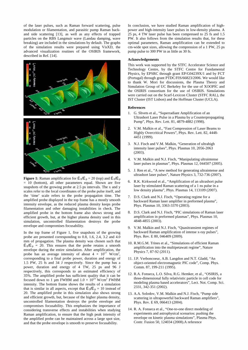
of the laser pulses, such as Raman forward scattering, pulse modulation or filamentation, and parasitic pump Raman back- and side scattering [13], as well as any effects of trapped particles on the RBS Langmuir wave (Landau damping, wave breaking) are included in the simulations by default. The graphs of the simulation results were prepared using VisXD, the advanced visualization routines of the OSIRIS framework, described in Ref. [14].

Figure 1: Raman amplification for É 0/É p = 20 (top) and É 0/Ép = 10 (bottom), all other parameters equal. Shown are five snapshots of the growing probe at 2.5 ps intervals. The x and y scales refer to the local coordinates of the probe pulse itself, and the ‘time’ scale refers to the probe propagation time. The amplified probe displayed in the top frame has a mostly smooth intensity envelope, as the reduced plasma density keeps probe filamentation and other damaging instabilities in check. The amplified probe in the bottom frame also shows strong and efficient growth, but, at the higher plasma density used in this simulation, uncontrolled filamentation destroys the probe envelope and compromises focusability.

In the top frame of Figure 1, five snapshots of the growing probe are presented corresponding to 0.8, 1.6, 2.4, 3.2 and 4.0 mm of propagation. The plasma density was chosen such that É 0/É p = 20. This ensures that the probe retains a smooth envelope during the entire simulation. After amplification, the probe has an average intensity of about 4 × 1017 W/cm2, corresponding to a final probe power, duration and energy of 1.5 PW, 25 fs and 34 J respectively. Since the pump has a power, duration and energy of 4 TW, 25 ps and 96 J respectively, this corresponds to an estimated efficiency of 35%. The amplified probe has sufficient quality that it can be focused down to 1 µm FWHM and 1.0 × 1023 W/cm2 FWHM intensity. The bottom frame shows the results of a simulation that is similar in all aspects, except that É 0/É p = 10 instead of 20. The amplified probe in this simulation also shows strong and efficient growth, but, because of the higher plasma density, uncontrolled filamentation destroys the probe envelope and compromises focusability. This emphasizes the importance of considering transverse effects and instabilities when studying Raman amplification, to ensure that the high peak intensity of the amplified probe can be maintained across a large spot size, and that the probe envelope is smooth to preserve focusability.

In conclusion, we have studied Raman amplification of high-power and high-intensity laser pulses in low-density plasma. A 25 ps, 4 TW laser pulse has been compressed to 25 fs and 1.5 PW. It also follows from the simulation results that, for these optimal parameters, Raman amplification can be extended to cm-wide spot sizes, allowing the compression of a 1 PW, 25 ps pump pulse to 300 PW in as little as 30 fs.

Acknowledgements

This work was supported by the STFC Accelerator Science and Technology Centre, by the STFC Centre for Fundamental Physics, by EPSRC through grant EP/G04239X/1 and by FCT (Portugal) through grant PTDC/FIS/66823/2006. We would like to thank W. Mori for discussions, the Plasma Theory and Simulation Group of UC Berkeley for the use of XOOPIC and the OSIRIS consortium for the use of OSIRIS. Simulations were carried out on the Scarf-Lexicon Cluster (STFC RAL), the IST Cluster (IST Lisbon) and the Hoffman Cluster (UCLA).

References

1. G. Shvets et al., “Superradiant Amplification of an Ultrashort Laser Pulse in a Plasma by a Counterpropagating Pump”, Phys. Rev. Lett. 81, 4879-4882 (1998).

2. V.M. Malkin et al., “Fast Compression of Laser Beams to Highly Overcritical Powers”, Phys. Rev. Lett. 82, 4448-4451 (1999).

3. N.J. Fisch and V.M. Malkin, “Generation of ultrahigh intensity laser pulses”, Phys. Plasmas 10, 2056-2063 (2003).

4. V.M. Malkin and N.J. Fisch, “Manipulating ultraintense laser pulses in plasmas”, Phys. Plasmas 12, 044507 (2005).

5. J. Ren et al., “A new method for generating ultraintense and ultrashort laser pulses”, Nature Physics 3, 732-736 (2007).

6. R.K. Kirkwood et al., “Amplification of an ultrashort pulse laser by stimulated Raman scattering of a 1 ns pulse in a low density plasma”, Phys. Plasmas 14, 113109 (2007).

7. D.S. Clark and N.J. Fisch, “Operating regime for a backward Raman laser amplifier in preformed plasma”, Phys. Plasmas 10, 3363-3370 (2003).

8. D.S. Clark and N.J. Fisch, “PIC simulations of Raman laser amplification in preformed plasmas”, Phys. Plasmas 10, 4848-4855 (2003).

9. V.M. Malkin and N.J. Fisch, “Quasitransient regimes of backward Raman amplification of intense x-ray pulses”, Phys. Rev. E 80, 046409 (2009).

10. R.M.G.M. Trines et al., “Simulations of efficient Raman amplification into the multipetawatt regime”, Nature Physics 7, 87-92 (2011).

11. J.P. Verboncoeur, A.B. Langdon and N.T. Gladd, “An object-oriented electromagnetic PIC code”, Comp. Phys. Comm. 87, 199-211 (1995).

12. R.A. Fonseca, L.O. Silva, R.G. Hemker, et al., “OSIRIS, a three-dimensional fully relativistic particle in cell code for modeling plasma based accelerators”, Lect. Not. Comp. Sci. 2331, 342-351 (2002).

13. A.A. Solodov, V.M. Malkin and N.J. Fisch, “Pump side scattering in ultrapowerful backward Raman amplifiers”, Phys. Rev. E 69, 066413 (2004).

14. R. A. Fonseca et al., “One-to-one direct modeling of experiments and astrophysical scenarios: pushing the envelope on kinetic plasma simulations”, Plasma Phys. Contr. Fusion 50, 124034 (2008).A reference

Use of the Debye-Waller Factor as a Temperature Diagnostic in Strongly Coupled Non-Equilibrium Plasmas.

T. G. White, J. Mithen, C. D. Murphy, G. Gregori Clarendon Laboratory, University of Oxford

D. Hochhaus, P. Neumayer GSI Helmholtzzentrum fr Schwerionenforschung GmbH

P. Davis, S. H. Glenzer, T. Ma, S. Le Pape Lawrence Livermore National Laboratory

B. Crowley AWE, Aldermaston

Introduction A complete description of the ion dynamics within the

warm dense matter (WDM) regime is important for describing many physical phenomena ranging from phase transitions within the interior of large astrophysical objects [1] to temperature relaxation rates during the internal processes of inertial confinement fusion [2]. Recent advances in both experimental and theoretical high energy density physics [3] have permitted these extreme states of matter to be formed in the laboratory and characterization methods are being rapidly developed and improved upon. Here we look at adapting a conventional condensed matter technique to study ion dynamics in the WDM state. This state is characterized by high pressure (≈1 Mbar), temperature (≈1 eV) and approximately solid density [4, 5] and represents a major challenge theoretically, computationally and experimentally. It lies in the regime between traditional solid state and plasma physics where expansion techniques are no longer applicable and neither the kinetic nor the potential energy can be treated perturbatively.

High density plasmas can be parameterized by the ion-ion coupling parameter,

(1) where Q is the ionic charge, Ti(e) the ion (electron)

temperature, a=(3/4πn)1/3 the Wigner-Seitz radius (average inter-particle separation) and n the ion number density. Equation (1) expresses the ratio of the pairwise Coulomb interaction to the average kinetic energy. WDM lies in the region where the coupling parameter is of order unity or greater. In this state strongly coupled ions, non-equilibrium species (Te/Ti > 1) and non-negligible electron degeneracy play an important role in defining structural dynamics [6]. At higher ion-ion coupling parameters the influence of the Coulomb interaction is increased and the ions arrange themselves around their equilibrium lattice positions. The ions oscillate around these positions and consequentially the ion acoustic waves present in a less strongly coupled plasma (fluid) are now replaced by phonons which must be treated quantum mechanically.

In the laboratory these non-equilibrium systems can occur when matter is exposed to ultra-intense optical laser radiation. Energy is transferred ‘instantaneously’ to the electrons in the system and the degree of electron-phonon coupling determines the inter-species temperature relaxation rates. One area that has received considerable attention and is based on these equilibration rates is the process of ultra-fast non-thermal `melting` [7, 8]. Here an ultra intense laser beam can create a strongly perturbed potential surface (due to the excited state of the energetic electrons) causing high carrier density and in some cases exceeding that of the crystal stability limit. The residual motion of the atoms then causes disordering

of the crystal on timescales much shorter than the usual propagation of a melt front. Conversely in gold the electron excitation is thought to produce a hardening of the lattice structure [9]. In all cases study into these non-equilibrium processes require simultaneous measurement of the electron and ion temperatures.

Currently many techniques exist to determine the electron temperature in a dense plasma [10]. However diagnosing the ion temperature, particularly at temperatures of a few eV or below, is far more difficult without resorting to interpolation based surface techniques such as emission spectroscopy [11], and interferometery [12, 13]. The method investigated in this report directly measures the ion bulk temperature through x-ray scattering from a strongly coupled plasma. The Debye-Waller (DW) technique has long been used in solid state physics as a way to characterize the displacement of atoms in a crystal from equilibrium through the intensity of elastically scattered radiation (Bragg diffraction) [14]. Here we examine the applicability of this technique to infer ion dynamics and temperature in matter transitioning from cold condensed matter to the WDM state. This is done through a combination of the solid state DW theory (section 1) and large-scale molecular dynamic simulation (section 2). Finally we evaluate the applicability of this technique through experimental results from proton heated highly orientated pyrolytic graphite (HOPG) (section 3).

1. Temperature Dependent Debye-Waller Factor In the kinematic limit where radiation interacts only

weakly with a sample it has been shown that the intensity of scattered radiation at position R is proportional to the value of the dynamic structure factor S, the incident power P0 and the inverse irradiated area A,

(2)

where ω is the frequency shift of the scattered photon and Ω the solid angle [10]. In the non-relativistic limit for near-elastic scattering, |k|=2k0sin(θ/2) for incident x-rays with wave vector |k0|=4π/λ0. Here, θ is the scattering angle and λ0 the probe wavelength. The dynamic structure factor is the spatial and temporal Fourier transform of the dynamic electron density-density auto-correlation function, known as the van Hove function [15]. In effect, the scattered radiation profile from a dense plasma contains information on the motion and position of the particles within.

In a solid it is natural to decompose the motion of the ions into multiple terms, Ri which represents the equilibrium position of the ions in the lattice as well as uoi(t) and uti(t) which represent the displacement of ions from these points, oscillatory and translational motion respectively. Following the derivation by Gregori [16, 17] we derive a set of equations

Γ =Q2

4π0kBTia,

Ps(R,ω)dΩdω ∝ P0

AS(k,ω) ,

Contact thomas.white@physics.ox.ac.uk

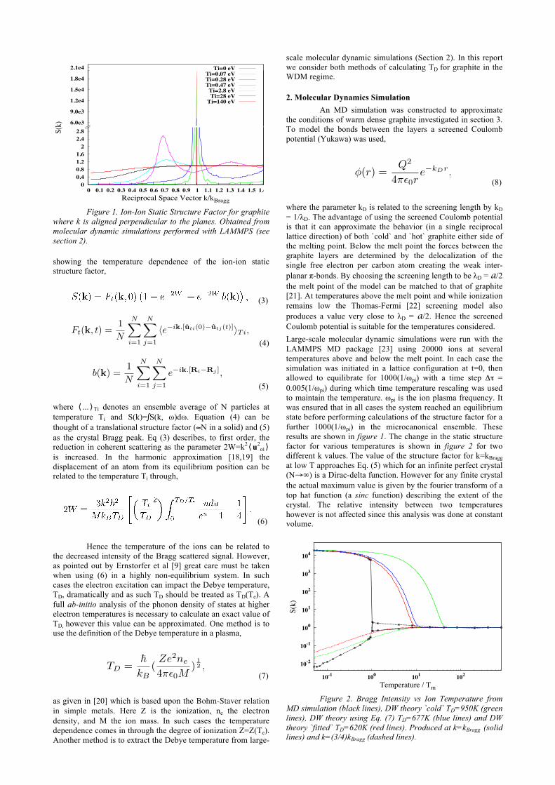
Figure 1. Ion-Ion Static Structure Factor for graphite

where k is aligned perpendicular to the planes. Obtained from molecular dynamic simulations performed with LAMMPS (see section 2).

showing the temperature dependence of the ion-ion static structure factor,

(3)

(4)

(5)

where ⟨...⟩Ti denotes an ensemble average of N particles at temperature Ti and S(k)=∫S(k, ω)dω. Equation (4) can be thought of a translational structure factor (≈N in a solid) and (5) as the crystal Bragg peak. Eq (3) describes, to first order, the reduction in coherent scattering as the parameter 2W=k2⟨u2

oi⟩ is increased. In the harmonic approximation [18,19] the displacement of an atom from its equilibrium position can be related to the temperature Ti through,

(6) Hence the temperature of the ions can be related to

the decreased intensity of the Bragg scattered signal. However, as pointed out by Ernstorfer et al [9] great care must be taken when using (6) in a highly non-equilibrium system. In such cases the electron excitation can impact the Debye temperature, TD, dramatically and as such TD should be treated as TD(Te). A full ab-initio analysis of the phonon density of states at higher electron temperatures is necessary to calculate an exact value of TD, however this value can be approximated. One method is to use the definition of the Debye temperature in a plasma,

(7)

as given in [20] which is based upon the Bohm-Staver relation in simple metals. Here Z is the ionization, ne the electron density, and M the ion mass. In such cases the temperature dependence comes in through the degree of ionization Z=Z(Te). Another method is to extract the Debye temperature from large-

scale molecular dynamic simulations (Section 2). In this report we consider both methods of calculating TD for graphite in the WDM regime.

2. Molecular Dynamics Simulation An MD simulation was constructed to approximate the conditions of warm dense graphite investigated in section 3. To model the bonds between the layers a screened Coulomb potential (Yukawa) was used,

(8) where the parameter kD is related to the screening length by kD = 1/λD. The advantage of using the screened Coulomb potential is that it can approximate the behavior (in a single reciprocal lattice direction) of both `cold` and `hot` graphite either side of the melting point. Below the melt point the forces between the graphite layers are determined by the delocalization of the single free electron per carbon atom creating the weak inter-planar π-bonds. By choosing the screening length to be λD = a/2 the melt point of the model can be matched to that of graphite [21]. At temperatures above the melt point and while ionization remains low the Thomas-Fermi [22] screening model also produces a value very close to λD = a/2. Hence the screened Coulomb potential is suitable for the temperatures considered. Large-scale molecular dynamic simulations were run with the LAMMPS MD package [23] using 20000 ions at several temperatures above and below the melt point. In each case the simulation was initiated in a lattice configuration at t=0, then allowed to equilibrate for 1000(1/ωpi) with a time step Δτ = 0.005(1/ωpi) during which time temperature rescaling was used to maintain the temperature. ωpi is the ion plasma frequency. It was ensured that in all cases the system reached an equilibrium state before performing calculations of the structure factor for a further 1000(1/ωpi) in the microcanonical ensemble. These results are shown in figure 1. The change in the static structure factor for various temperatures is shown in figure 2 for two different k values. The value of the structure factor for k=kBragg at low T approaches Eq. (5) which for an infinite perfect crystal (N→∞) is a Dirac-delta function. However for any finite crystal the actual maximum value is given by the fourier transform of a top hat function (a sinc function) describing the extent of the crystal. The relative intensity between two temperatures however is not affected since this analysis was done at constant volume.

Figure 2. Bragg Intensity vs Ion Temperature from

MD simulation (black lines), DW theory `cold` TD=950K (green lines), DW theory using Eq. (7) TD=677K (blue lines) and DW theory `fitted` TD=620K (red lines). Produced at k=kBragg (solid lines) and k=(3/4)kBragg (dashed lines).

6.0e3

9.0e3

1.2e4

1.5e4

1.8e4

2.1e4 Ti=0 eV Ti=0.07 eV Ti=0.28 eV Ti=0.47 eV Ti=2.8 eV Ti=28 eV

Ti=140 eV

00.40.81.21.6

22.42.8

0 0.1 0.2 0.3 0.4 0.5 0.6 0.7 0.8 0.9 1 1.1 1.2 1.3 1.4 1.5 1.6

S(k)

Reciprocal Space Vector k/kBragg

Ft(k, t) =1

N

N

i=1

N

j=1

e−ik.[uti(0)−utj(t)]Ti,

b(k) =1

N

N

i=1

N

j=1

e−ik.[Ri−Rj ],

TD =kB

(Ze2ne

4π0M)

12 ,

φ(r) =Q2

4π0re−kDr,

10-2

10-1

100

101

102

103

104

10-1 100 101 102

S(k)

Temperature / Tm

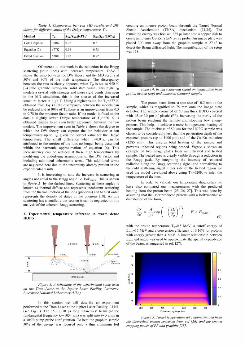
Table 1. Comparison between MD results and DW theory for different values of the Debye temperature, TD.

Method TD SMD/SDW(0.5TM) SMD/SDW(0.9TM)

Cold Graphite 950K 0.75 0.5

Equation (7) 677K 0.94 0.78

Fitted function 620K 1.02 0.92

Of interest to this work is the reduction in the Bragg scattering (solid lines) with increased temperature. Table 1 shows the ratio between the DW theory and the MD results at 50% and 90% of the melt temperature. The discrepancy between the two is clearly apparent when TD is set to 950 K [24] the graphite inter-plane solid state value. This high TD models a crystal with stronger and more rigid bonds than seen in the MD simulation, this is the source of the increased structure factor at high T. Using a higher value for TD=677 K obtained from Eq. (7) the discrepancy between the models can be reduced and at 90% of Tm there is an improvement from 0.5 to 0.78 in the structure factor ratio. If the model is fitted to the data a slightly lower Debye temperature of TD=620 K is obtained leading to an even better agreement between the two models. The improvement seen in Table 1 shows the degree to which the DW theory can capture the ion behavior at ion temperatures up to Tm given the correct value for the Debye temperature. The small difference when T=0.9TM can be attributed to the motion of the ions no longer being described within the harmonic approximation of equation (6). This inconsistency can be reduced at these high temperatures by modifying the underlying assumptions of the DW factor and including additional anharmonic terms. This additional terms are neglected here due to the uncertainty already present in the experimental results.

It is interesting to note the increase in scattering at angles not equal to the Bragg angle i.e. k≠kBragg. This is shown in figure 2 by the dashed lines. Scattering at these angles is known as thermal diffuse and represents incoherent scattering from the thermal motion of the ions (phonons) and to first order represents the density of states of the phonons [18]. As this scattering has a smaller cross section it can be neglected in this analysis of the coherent Bragg scattering.

3. Experimental temperature inference in warm dense HOPG

Figure 3. A schematic of the experimental setup used

on the Titan Laser at the Jupiter Laser Facility, Lawrence Livermore National Laboratory (USA).

In this section we will describe an experiment performed at the Titan Laser at the Jupiter Laser Facility, LLNL (see Fig 3). The 150 J, 10 ps long Titan west beam (at the fundamental frequency λ0=1054 nm) was split into two arms in a 30/70 pump-probe configuration. To heat the graphite sample 30% of the energy was focused onto a thin aluminum foil

creating an intense proton beam through the Target Normal Sheath Acceleration (TNSA) mechanism [24,25]. The remaining energy was focused 225 ps later onto a copper disk to create an intense Cu-Kα 8 keV x-ray probe. An image plate was placed 300 mm away from the graphite sample at 27.4° to detect the Bragg diffracted light. The magnification of the setup was 138.

Figure 4. Bragg scattering signal on image plate from proton heated (top) and unheated (bottom) sample.

The proton beam forms a spot size of ~0.5 mm on the sample, which is magnified to 75 mm onto the image plate detector. The sample consisted of 50 µm thick HOPG covered with 15 or 30 µm of plastic (PP), increasing the purity of the proton beam reaching the sample and stopping low energy protons. This helps to achieve a more homogeneous heating of the sample. The thickness of 50 µm for the HOPG sample was chosen to be considerably less than the penetration depth of the expected protons (up to 1000 µm) and of the Cu-Kα radiation (1285 µm). This ensures total heating of the sample and prevents unheated regions being probed. Figure 4 shows an example of two image plates from an unheated and heated sample. The heated area is clearly visible through a reduction in the Bragg peak. By integrating the intensity of scattered radiation along the Bragg scattering signal and normalizing to the cold scattering signal either side of the heated region we used the model developed above using TD=620K to infer the temperature of the ions.

In order to validate our temperature diagnostics we have also compared our measurements with the predicted heating from the proton beam [25, 26, 27]. This was done by assuming that the laser produced protons with a Boltzmann-like distribution of the form,

(9)

with the proton temperature Tp≈0.5 MeV, a cutoff energy of Emax≈15 MeV and a conversion efficiency of 0.16% for protons with energy greater than 4 MeV. A linear relationship between Emax and angle was used to approximate the spatial dependence of the beam, as suggested in ref. [27].

Figure 5. Target temperature (eV) approximated from

the theoretical proton spectrum from ref [26] and the known stopping power of PP and graphite [28].

dN

dE=

A

E12

exp

−2E

Tp

12

E < Emax ,

From the assumed proton distribution and its spatial variation using the known stopping power in cold PP and graphite the estimated deposited energy at a given depth in the sample was calculated. An example for 15 µm of PP is given in figure 5 with the resulting heating profiles shown for the different cases in figure 6. Figure 6 also shows the temperatures obtained for three different shots using the DW theory for 15 µm of PP (a), 30 µm of PP (b) and no proton beam (c). The similarity between the temperatures obtained using the theoretical spectrum and those obtained using the DW theory coupled with the experimental results is promising. Further analysis of the proton spectrum using RCF and proton spectrometers present at the experiment should allow for improvement between the predicted and the measured temperatures in the sample. This analysis should help to evaluate the validity of the spatial features of the heated sample present in our results.

Figure 6. Inferred ion temperature from the DW

model (red lines) and expected temperature from the theoretical proton spectrum (blue lines) for 15 µm of PP (a), 30 µm of PP (b) and no heating (c). The red dashed line indicates the equilibrium melt temperature of graphite ~0.33 eV. Conclusions

In this report we present an overview of the Debye-Waller (DW) technique to characterize the displacement of atoms in a crystal from the equilibrium positions. We show how within the harmonic approximation this displacement can be linked to the ion temperature through eq. (6) provided that

TD is known. Using a classical simulation we have shown that when a fitted TD is used the DW theory agrees with MD simulation extremely well up to 90% of the melt temperature, Tm. However when using the solid state result we obtained a large (~50%) discrepancy at these higher temperatures. We also showed that for temperatures below 0.5Tm using the value of TD obtained from the the Bohm-Staver relation (7) is also comparatively accurate (<5%).

Finally we evaluate the validity of this technique through experimental results in an equilibrium system by inferring the ion temperature in warm dense graphite (HOPG) and have shown that the results obtained from the DW theory compare favorably with an approximate proton spectrum and known energy deposition in graphite.

Acknowledgements The work in this report was supported by funding from AWE. The author would also like to thank all the staff at the Jupiter Laser Facility, LLNL for their support.

References [1] J. Daligault and S. Gupta, Astrophys.J. 703, 994 (2009). [2] M. Matzen, M. Sweeney, R. Adams, and J. Asay, Physics of Plasmas (2005). [3] R. Drake, High-energy-density physics, fundamentals, inertial fusion, and experimental astrophysics (Springer Verlag, 2006). [4] R. Davidson, D. Arnett, J. Dahlburg, and P. Dimotakis, Frontiers in high energy density physics (Frontiers, 2002). [5] R. Drake, Physics Of Plasmas 16, 055501 (2009). [6] G. Gregori and D.O. Gericke. Physics Of Plasmas. 16, 5 (2009) [7] C.W. Siders, Science 286, 1340 (1999). [8] A. M. Lindenberg, Science 308, 392 (2005). [9] R. Ernstorfer et al, Science 323, 5917 (2009) . [10] S.H. Glenzer and R. Redmer, Reviews Of Modern Physics 81, 1625 (2009). [11] P. Patel et al, Physical Review Letters 91, 12, (2003). [12] A. Mancic et al, High Energy Density Physics 6, 21 (2010). [13] G.M. Dyer et al, Physical Review Letters 101, 1, (2008). [14] T.H. Metzger, Journal of Applied Crystallography 19, 200 (1986). [15] J.P. Hansen and I. R. McDonald, Theory of Simple Liquids, Third Edition, 3rd ed. (Academic Press, 2006). [16] G. Gregori, S. Glenzer, W. Rozmus, R. Lee, and O. Landen, Physical Review E 67, 026412 (2003). [17] G. Gregori, S. H. Glenzer, and O. L. Landen, Physical Review E 74, 026402 (2006). [18] J. Als-Nielsen, Elements of Modern X-Ray Physics (Wiley, John & Sons, Incorporated, 2001). [19] R. Mossbauer and W. Wiedemann. Kernresonanzabsorption Nicht Doppler-Verbreiterter Gammastrahlung in Re-187. Z Phys. 159, 1 (1960). [20] G. Gregori et al, High Energy Density 3, 99 (2007). [21] S. Hamaguchi, R. Farouki, and D. Dubin, Physical Review E 56, 4671 (1997). [22] D. Salzmannn, Atomic Physics in Hot Plasmas (Oxford University Press, 1998) [23] http://lammps.sandia.gov/ [24] W. DeSorbo, The Specific Heat of Graphite from 13° to 300°K. J. Chem. Phys. 21, 1660 (1953). [25] P. Mora, Plasma Expansion into a Vacuum. Physical Review Letters. 90, 18 (2003). [26] J. Fuchs et al, Laser-driven proton scaling laws and new paths towards energy increase. Nat Phys. 2, 48–54. (2006). [27] F.Nuernberg, M. Schollmeier, E. Brambrink, et al. Radiochromic film imaging spectroscopy of laser-accelerated proton beams. Rev Sci Instrum. 80, 3 (2009) [28] http://physics.nist.gov/PhysRefData/Star/Text/PSTAR.html

0

0.05

0.1

0.15

0.2

0.25

0.3

0.35

0.4

-0.8 -0.6 -0.4 -0.2 0 0.2 0.4 0.6 0.8

Infer

red I

on T

empe

ratur

e (eV

)

Distance on HOPG (mm)

0

0.05

0.1

0.15

0.2

0.25

0.3

0.35

0.4

-0.8 -0.6 -0.4 -0.2 0 0.2 0.4 0.6 0.8

Infer

red I

on T

empe

ratur

e (eV

)

Distance on HOPG (mm)

0

0.05

0.1

0.15

0.2

0.25

0.3

0.35

0.4

-0.8 -0.6 -0.4 -0.2 0 0.2 0.4 0.6 0.8

Infer

red I

on T

empe

ratur

e (eV

)

Distance on HOPG (mm)

(a)

(b)

(c)

Gaps in data correspond to no scattered light i.e. to graphite above

the melt point

A new VFP-PIC hybrid code to model fast electron transport with hydrodynamic response

B. E. R. Williams and R. J. Kingham

Imperial College of Science Technology and Medicine London, SW7 2AZ

Introduction

The interaction of a high-intensity laser beam with a solid target generates a large number of fast-electrons with long mean free paths. The study of these fast-electrons is still the subject of active research, given their relevance to Tabak's proposed fast-ignition (FI) approach to inertial confinement fusion [1]. Modelling of these electrons from the region in which they are generated to the dense fuel core is not a trivial task given the range of plasma conditions experienced by the electrons. Conventional methods for simulating this FI system fall into two categories: kinetic and hybrid codes. Kinetic codes, such as Vlasov Fokker-Planck (VFP) and Particle in Cell (PIC) codes, provide an almost complete description of the system, but are often computationally expensive and have strict constraints on the time-step. Thus, these codes can struggle to model picosecond timescales when hydrodynamics of the background is expected to be significant. VFP codes work best in collision-dominated plasmas. As for PIC codes, there is some debate about their ability to reproduce the results of classical transport theory, which can play a significant role in beam-plasma systems. Furthermore, PIC codes can struggle to accurately represent the fast-electron beam in a solid density background as most of the particles in a cell will be used to model the background. Hybrid codes [2] often consist of a PIC code, which accurately models the fast-electrons, and a simple fluid code to model the response of the background. While hybrid codes are computationally light, the description of the background is often rudimentary. This reduced description of the background allows probing of longer time-scales and larger spatial-scales. This description of the background is sometimes as simple as

where η is the Spitzer resistivity. However, η should be a tensor when magnetic fields are present [3]. Also this simple treatment neglects many terms present in the full Ohm’s law. More advanced hybrid codes still rely on the fluid treatment of the background plasma. However this treatment is only valid in the case of Maxwellian background distribution functions and also in the absence of steep number density and temperature gradients. Both non-Maxwellian distributions and steep gradients are expected to be present in fast ignition scenario.

Novel Hybrid Code

We present a new approach to modeling fast ignition type scenarios. This novel hybrid code offers a good description of the fast-electrons (PIC), and an improved description of the background (VFP) compared to conventional hybrid codes. The VFP code used (IMPACT [4]) is suited to describing magnetized transport in the presence of steep temperature and number density gradients. Furthermore, it can model magnetic field generation and includes the displacement current in Ampere’s law. IMPACT solves the VFP equation by making use of a Cartesian tensor expansion in velocity space

In order to truncate this expansion, IMPACT utilises the diffusion approximation, which neglects terms in f of higher order than 1. This approximation is valid for a collisional plasma, and limits the hybrid approach to systems with small beam to background ratios (just as in a conventional hybrid code). The PIC code and VFP code are linked via their current contributions to Ampere’s law.

Filamentation instability

To test the VFP-PIC interaction we considered the filamentation instability in a 1d2v system. The mechanism for this instability is essentially a feedback between the generation of a magnetic field due a transverse perturbation of the beam current, and the enhancement of this current due to the Lorentz force of the perturbed magnetic field [5]. Due to the novel set up of the hybrid scheme it was necessary to derive a dispersion relation in the VFP-PIC system. We used the approach of Epperlein [6] as a template. We consider the distribution function of the background electrons to be a shifted Maxwellian evolving under the f0 and f1 equations. The beam electrons are initially monokinetic with velocity vh and evolve under the collisionless Vlasov equation. Considering wavelike perturbations, and using Ampere’s law and Faraday’s law we find a cubic dispersion relation of the form given in figure

where

and

γ is the growth rate, k is the wavenumber of the instability,

ωh is the hot electron plasma frequency,

ωc is the background

electron plasma frequency,

τ th is the collision time of a thermal electron in the background,

f00 is the initial isotropic part of the

distribution function for the background electrons. The real parts of the roots of the above cubic are shown in figure 1 for a system with a beam to background ratio of 0.01, vh = 10 vth, where vth is the thermal velocity in the background, with the background at a temperature of 50 eV and an electron density of and 5*1021 /cm3.

Contact brennig.williams08@imperial.ac.uk

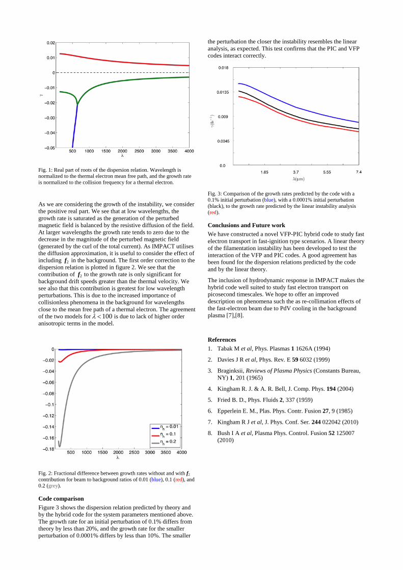
Fig. 1: Real part of roots of the dispersion relation. Wavelength is normalized to the thermal electron mean free path, and the growth rate is normalized to the collision frequency for a thermal electron.

As we are considering the growth of the instability, we consider the positive real part. We see that at low wavelengths, the growth rate is saturated as the generation of the perturbed magnetic field is balanced by the resistive diffusion of the field. At larger wavelengths the growth rate tends to zero due to the decrease in the magnitude of the perturbed magnetic field (generated by the curl of the total current). As IMPACT utilises the diffusion approximation, it is useful to consider the effect of including f2 in the background. The first order correction to the dispersion relation is plotted in figure 2. We see that the contribution of f2 to the growth rate is only significant for background drift speeds greater than the thermal velocity. We see also that this contribution is greatest for low wavelength perturbations. This is due to the increased importance of collisionless phenomena in the background for wavelengths close to the mean free path of a thermal electron. The agreement of the two models for

λ <100 is due to lack of higher order anisotropic terms in the model.

Fig. 2: Fractional difference between growth rates without and with f2 contribution for beam to background ratios of 0.01 (blue), 0.1 (red), and 0.2 (grey).

Code comparison

Figure 3 shows the dispersion relation predicted by theory and by the hybrid code for the system parameters mentioned above. The growth rate for an initial perturbation of 0.1% differs from theory by less than 20%, and the growth rate for the smaller perturbation of 0.0001% differs by less than 10%. The smaller

the perturbation the closer the instability resembles the linear analysis, as expected. This test confirms that the PIC and VFP codes interact correctly.

Fig. 3: Comparison of the growth rates predicted by the code with a 0.1% initial perturbation (blue), with a 0.0001% initial perturbation (black), to the growth rate predicted by the linear instability analysis (red).

Conclusions and Future work

We have constructed a novel VFP-PIC hybrid code to study fast electron transport in fast-ignition type scenarios. A linear theory of the filamentation instability has been developed to test the interaction of the VFP and PIC codes. A good agreement has been found for the dispersion relations predicted by the code and by the linear theory.

The inclusion of hydrodynamic response in IMPACT makes the hybrid code well suited to study fast electron transport on picosecond timescales. We hope to offer an improved description on phenomena such the as re-collimation effects of the fast-electron beam due to PdV cooling in the background plasma [7],[8].

References

1. Tabak M et al, Phys. Plasmas 1 1626A (1994)

2. Davies J R et al, Phys. Rev. E 59 6032 (1999)

3. Braginksii, Reviews of Plasma Physics (Constants Bureau, NY) 1, 201 (1965)

4. Kingham R. J. & A. R. Bell, J. Comp. Phys. 194 (2004)

5. Fried B. D., Phys. Fluids 2, 337 (1959)

6. Epperlein E. M., Plas. Phys. Contr. Fusion 27, 9 (1985)

7. Kingham R J et al, J. Phys. Conf. Ser. 244 022042 (2010)

8. Bush I A et al, Plasma Phys. Control. Fusion 52 125007 (2010)