Embed Size (px)
Citation preview
Introduction to
PLASMA ASTROPHYSICS
(Selected 10 lectures)
Boris V. Somov
Astronomical Institute and Faculty of Physics
Moscow State University
Pushino-na-Oke, 2008
Contents
About These Lectures 5
1 Particles and Fields: Exact Self-Consistent Description 91.1 Liouville’s theorem . . . . . . . . . . . . . . . . . . . 9
1.1.1 Continuity in phase space . . . . . . . . . 91.1.2 The character of particle interactions 121.1.3 The Lorentz force, gravity . . . . . . . . . 151.1.4 Collisional friction . . . . . . . . . . . . . . . 161.1.5 The exact distribution function . . . . 18
1.2 Charged particles in the electromagnetic field . . . . . . . . . 221.2.1 General formulation of the problem . 221.2.2 The continuity equation for electric
charge . . . . . . . . . . . . . . . . . . . . . . . . . 241.2.3 Initial equations and initial conditions 251.2.4 Astrophysical plasma applications . . 26
1.3 Gravitational systems . . . . . . . . . . . . . . . . . . . . . . 281.4 Practice: Exercises and Answers . . . . . . . . . . . . . . . . 29
2 Statistical Description of Interacting Particle Systems 332.1 The averaging of Liouville’s equation . . . . . . . . . . . . . . 33
2.1.1 Averaging over phase space . . . . . . . . 332.1.2 Two statistical postulates . . . . . . . . . 352.1.3 A statistical mechanism of mixing . . 372.1.4 Derivation of a general kinetic equa-
tion . . . . . . . . . . . . . . . . . . . . . . . . . . . 402.2 A collisional integral and correlation functions . . . . . . . . . 43
2.2.1 Binary interactions . . . . . . . . . . . . . . . 432.2.2 Binary correlation . . . . . . . . . . . . . . . 46
1
2 CONTENTS
2.2.3 The collisional integral and binarycorrelation . . . . . . . . . . . . . . . . . . . . . . 48
2.3 Equations for correlation functions . . . . . . . . . . . . . . . 512.4 Practice: Exercises and Answers . . . . . . . . . . . . . . . . 54
3 Weakly-Coupled Systems with Binary Collisions 553.1 Approximations for binary collisions . . . . . . . . . . . . . . 55
3.1.1 The small parameter of kinetic theory 553.1.2 The Vlasov kinetic equation . . . . . . . 583.1.3 The Landau collisional integral . . . . . 593.1.4 The Fokker-Planck equation . . . . . . . 61
3.2 Correlations and Debye-Huckel shielding . . . . . . . . . . . . 643.2.1 The Maxwellian distribution function 643.2.2 The averaged force and electric neu-
trality . . . . . . . . . . . . . . . . . . . . . . . . . 653.2.3 Pair correlations and the Debye-Huckel
radius . . . . . . . . . . . . . . . . . . . . . . . . . 673.3 Gravitational systems . . . . . . . . . . . . . . . . . . . . . . 703.4 Comments on numerical simulations . . . . . . . . . . . . . . 713.5 Practice: Exercises and Answers . . . . . . . . . . . . . . . . 73
4 Macroscopic Description of Astrophysical Plasma 774.1 Summary of microscopic description . . . . . . . . . . . . . . 774.2 Definition of macroscopic quantities . . . . . . . . . . . . . . 784.3 Macroscopic transfer equations . . . . . . . . . . . . . . . . . 80
4.3.1 Equation for the zeroth moment . . . . 804.3.2 The momentum conservation law . . . 82
4.4 The energy conservation law . . . . . . . . . . . 864.4.1 The second moment equation . . . . . . 864.4.2 The case of thermodynamic equilib-
rium . . . . . . . . . . . . . . . . . . . . . . . . . . . 894.4.3 The general case of anisotropic plasma 90
4.5 General properties of transfer equations . . . . . . . . . . . . 924.5.1 Divergent and hydrodynamic forms . 924.5.2 Status of the conservation laws . . . . . 94
4.6 Equation of state and transfer coefficients . . . . . . . . . . . 954.7 Gravitational systems . . . . . . . . . . . . . . . . . . . . . . 98
CONTENTS 3
5 The Generalized Ohm’s Law in Plasma 1015.1 The classic Ohm’s law . . . . . . . . . . . . . . . . . . . . . . 1015.2 Derivation of basic equations . . . . . . . . . . . . . . . . . . 1025.3 The general solution . . . . . . . . . . . . . . . . . . . . . . . 1065.4 The conductivity of magnetized plasma . . . . . . . . . . . . 107
5.4.1 Two limiting cases . . . . . . . . . . . . . . . 1075.4.2 The physical interpretation . . . . . . . . 108
5.5 Currents and charges in plasma . . . . . . . . . . . . . . . . . 1115.5.1 Collisional and collisionless plasmas . 1115.5.2 Volume charge and quasi-neutrality . 115
5.6 Practice: Exercises and Answers . . . . . . . . . . . . . . . . 117
6 Single-Fluid Models for Astrophysical Plasma 1196.1 Derivation of the single-fluid equations . . . . . . . . . . . . . 119
6.1.1 The continuity equation . . . . . . . . . . . 1196.1.2 The momentum conservation law . . . 1206.1.3 The energy conservation law . . . . . . . 123
6.2 Basic assumptions and the MHD equations . . . . . . . . . . 1266.2.1 Old simplifying assumptions . . . . . . . 1266.2.2 New simplifying assumptions . . . . . . 1286.2.3 Non-relativistic MHD . . . . . . . . . . . . 1316.2.4 Energy conservation . . . . . . . . . . . . . . 1336.2.5 Relativistic magnetohydrodynamics . 134
6.3 Magnetic flux conservation. Ideal MHD . . . . . . . . . . . . 1356.3.1 Integral and differential forms of the
law . . . . . . . . . . . . . . . . . . . . . . . . . . . . 1356.3.2 The ideal MHD . . . . . . . . . . . . . . . . . 1396.3.3 The ‘frozen field’ theorem . . . . . . . . . 141
6.4 Magnetic reconnection . . . . . . . . . . . . . . . . . . . . . . 1436.5 Practice: Exercises and Answers . . . . . . . . . . . . . . . . 146
7 MHD in Astrophysics 1497.1 The main approximations in ideal MHD . . . . . . . . . . . . 149
7.1.1 Dimensionless equations . . . . . . . . . . 1497.1.2 Weak magnetic fields in astrophysi-
cal plasma . . . . . . . . . . . . . . . . . . . . . . 1527.1.3 Strong magnetic fields in plasma . . . 153
7.2 Accretion disks of stars . . . . . . . . . . . . . . . . . . . . . 1577.2.1 Angular momentum transfer . . . . . . . 157
4 CONTENTS
7.2.2 Accretion in cataclysmic variables . . 1597.2.3 Accretion disks near black holes . . . . 1607.2.4 Flares in accretion disk coronae . . . . 161
7.3 Astrophysical jets . . . . . . . . . . . . . . . . . . . . . . . . . 1627.3.1 Jets near black holes . . . . . . . . . . . . . 1627.3.2 Relativistic jets from disk coronae . . 165
7.4 Practice: Exercises and Answers . . . . . . . . . . . . . . . . 166
8 Plasma Flows in a Strong Magnetic Field 1698.1 The general formulation of a problem . . . . . . . . . . . . . 1698.2 The formalism of 2D problems . . . . . . . . . . . . . . . . . 172
8.2.1 The first type of problems . . . . . . . . . 1738.2.2 The second type of MHD problems . 175
8.3 The existence of continuous flows . . . . . . . . . . . . . . . . 1818.4 Flows in a time-dependent dipole field . . . . . . . . . . . . . 183
8.4.1 Plane magnetic dipole fields . . . . . . . 1838.4.2 Axial-symmetric dipole fields . . . . . . 188
8.5 Practice . . . . . . . . . . . . . . . . . . . . . . . . . . . . . . 191
About These Lectures
If you want to learn the most fundamental things about plasma as-trophysics with the least amount of time and effort – and whodoesn’t? – this text is for you.
The textbook is addressed to students without a background inplasma physics.
It grew from the lectures given at the Moscow Institute of Physicsand Technics (the ‘fiz-tekh’) since 1977.
A similar full-year course was offered to the students of the As-tronomical Division in the Faculty of Physics at the Moscow StateUniversity over the years after 1990.
The idea of the book is not typical for the majority of textbooks.
It was suggested by S.I. Syrovatskii that
the consecutive consideration of physical principles, start-ing from the most general ones, and of simplifying assump-tions gives us a simpler description of plasma under cosmicconditions.
On the basis of such an approach the student interested in modernastrophysics, its current practice, will find the answers to two keyquestions:
1. What approximation is the best one (the simplest but sufficient)for description of a phenomenon in astrophysical plasma?
5
6 About These Lectures
2. How can I build an adequate model for the phenomenon, forexample, a flare in the corona of an accretion disk?
Practice is really important for the theory of astrophysical plasma.
Related exercises (supplemented to each chapter) serve to betterunderstanding of plasma astrophysics.
As for the applications, preference evidently is given to physicalprocesses in the solar plasma.
Why? – Because of the possibility of the all-round observationaltest of theoretical models.
For instance, flares on the Sun, in contrast to those on other stars,can be seen in their development.
We can obtain a sequence of images during the flare’s evolution,not only in the optical and radio ranges but also in the EUV, soft andhard X-ray, gamma-ray ranges.
It is assumed that the students have mastered a course of generalphysics and have some initial knowledge of theoretical physics.
For beginning students, who may not know in which subfields ofastrophysics they wish to specialize,
it is better to cover a lot of fundamental theories thoroughlythan to dig deeply into any particular astrophysical subjector object,
even a very interesting one, for example black holes.
Astrophysicists of the future will need tools that allow them toexplore in many different directions.
Moreover astronomy of the future will be, more than hitherto, pre-cise science similar to mathematics and physics.
see http://www.springer/com/http://adsabs.harvard.edu/
About These Lectures 7
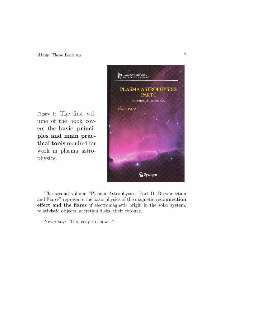
Figure 1: The first vol-ume of the book cov-ers the basic princi-ples and main prac-tical tools required forwork in plasma astro-physics.
The second volume “Plasma Astrophysics, Part II, Reconnectionand Flares” represents the basic physics of the magnetic reconnectioneffect and the flares of electromagnetic origin in the solar system,relativistic objects, accretion disks, their coronae.
Never say: “It is easy to show...”.
8 About These Lectures
Chapter 1
Particles and Fields: ExactSelf-Consistent Description
There exist two ways to describe exactly the behaviour ofa system of charged particles in electromagnetic and gravi-tational fields.
1.1 Liouville’s theorem
1.1.1 Continuity in phase space
Let us consider a system of N interacting particle.
Without much justification, let us introduce the distribution func-tion
f = f(r,v, t) (1.1)
for particles as follows.
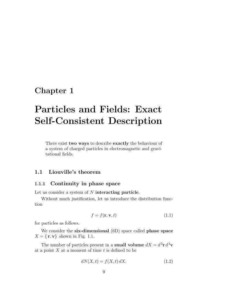
We consider the six-dimensional (6D) space called phase spaceX = r,v shown in Fig. 1.1.
The number of particles present in a small volume dX = d 3r d 3vat a point X at a moment of time t is defined to be
dN(X, t) = f(X, t) dX. (1.2)
9
10 Chapter 1. Particles and Fields
v
r0
X
d X
d
d3
3
v
r
X
Figure 1.1: The 6D phase space X. A small volume dX at apoint X.
Accordingly, the total number of the particles at this moment is
N(t) =∫
f(X, t) dX ≡∫ ∫
f(r,v, t) d 3r d 3v . (1.3)
If, for definiteness, we use the Cartesian coordinates, then
X = x, y, z, vx, vy, vz
is a point of the phase space (Fig. 1.2) and
X = vx, vy, vz, vx, vy, vz (1.4)
is the velocity of this point in the phase space.
Suppose the coordinates and velocities of the particles are chang-ing continuously – ‘from point to point’, i.e. the particles movesmoothly at all times.
So the distribution function f(X, t) is differentiable.
1.1. Liouville’s Theorem 11
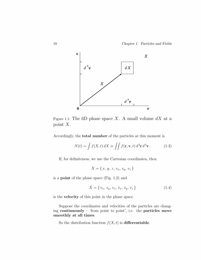
Moreover we assume that this motion of the particles in phase spacecan be expressed by the continuity equation:
∂f
∂t+ div
XfX = 0
(1.5)
or∂f
∂t+ divr fv + divv f v = 0 .
v
r0
X X
S
U
dS
.J
Figure 1.2: The 6D phase space X. The volume U is enclosedby the surface S.
Equation (1.5) expresses the conservation law for the particles,since the integration of (1.5) over a volume U enclosed by the surface Sin Fig. 1.2 gives
∂
∂t
∫
U
f dX +∫
U
divX
fX dX =
by virtue of the Ostrogradskii-Gauss theorem
12 Chapter 1. Particles and Fields
=∂
∂tN(t)
∣∣∣∣U
+∫
S
fX dS =∂
∂tN(t)
∣∣∣∣U
+∫
S
J · dS = 0 . (1.6)
HereJ = fX (1.7)
is the particle flux density in the phase space.
Thus
a change of the particle number in a given volume U of thephase space X is defined by the particle flux through theboundary surface S.
The reason is clear.
There are no sources or sinks for the particles inside the volume.
Otherwise the source and sink terms must be added to the right-hand side of Equation (1.5).
1.1.2 The character of particle interactions
Let us rewrite Equation (1.5) in another form in order to understandthe meaning of divergent terms.
The first of them is
divr fv = f divr v + (v · ∇r) f = 0 + (v · ∇r) f ,
since r and v are independent variables in the phase space X.
The second divergent term is
divv f v = f divv v + v · ∇v f .
So far no assumption has been made as to the character of par-ticle interactions.
1.1. Liouville’s Theorem 13
It is worth doing here.
Let us restrict our consideration to the interactions with
divv v = 0 ,(1.8)
then Equation (1.5) takes the following form
∂f
∂t+ v · ∇r f +
F
m· ∇v f = 0
or∂f
∂t+ X∇
Xf = 0 , (1.9)
where
X =
vx, vy, vz,Fx
m,
Fy
m,
Fz
m
. (1.10)
So we ‘trace’ the phase trajectories of particles when they moveunder action of a force field F(r,v, t).
Thus we have found Liouville’s theorem in the following formulation:
∂f
∂t+ v · ∇r f +
F
m· ∇v f = 0 . (1.11)
Liouville’s theorem: The distribution function remainsconstant on the particle phase trajectories if condition (1.8)is satisfied.
We call Equation (1.11) the Liouville equation.
The first term in Equation (1.11), the partial time derivative ∂f/∂t ,characterizes a change of the distribution function f(t,X) at a givenpoint X in the phase space with time t.
Define also the Liouville operator
14 Chapter 1. Particles and Fields
D
Dt≡ ∂
∂t+ X
∂
∂X≡ ∂
∂t+ v · ∇r +
F
m· ∇v . (1.12)
This operator is just the total time derivative following a particle mo-tion in the phase space X.
By using definition (1.12), we rewrite Liouville’s theorem as follows:
Df
Dt= 0 .
(1.13)
What factors do lead to the changes in the distribution function?
Let dX be a small volume in the phase space X.
v
r0
J
v
r0
Jr
v
Jr
Jv
v
FdX dX
(a) (b)
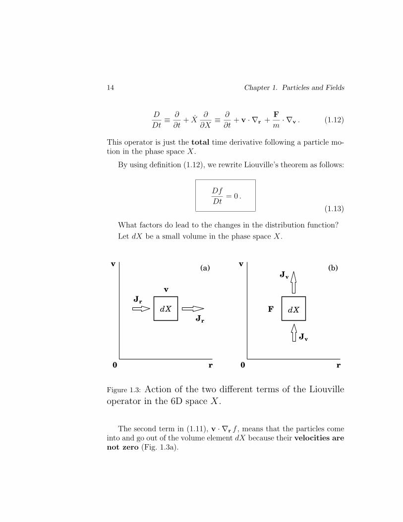
Figure 1.3: Action of the two different terms of the Liouvilleoperator in the 6D space X.
The second term in (1.11), v · ∇r f , means that the particles comeinto and go out of the volume element dX because their velocities arenot zero (Fig. 1.3a).
1.1. Liouville’s Theorem 15
So this term describes a simple kinematic effect.
If the distribution function f has a gradient over r, then anumber of particles inside the volume dX changes becausethey move with velocity v.
The third term, (F/m) ·∇v f , means that the particles escape fromthe volume element dX or come into it due to their acceleration ordeceleration under action of the force field F (Fig. 1.3b).
1.1.3 The Lorentz force, gravity
In order the Liouville theorem to be valid, the force field F has to satisfycondition (1.8).
We rewrite it as follows:
∂ vα
∂ vα
=1
m
∂Fα
∂ vα
= 0
or
∂Fα
∂ vα
= 0 , α = 1, 2, 3 . (1.14)
In particular, this condition holds if
the component Fα of the force vector F does not depend uponthe velocity component vα.
This is a sufficient condition, of course.
The classical Lorentz force
Fα = e[Eα +
1
c(v ×B )α
](1.15)
obviously has that property.
16 Chapter 1. Particles and Fields
The gravitational force in the classical approximation is entirelyindependent of velocity.
Other forces are considered, depending on a situation, e.g., theforce resulting from the emission of radiation (the radiation reaction)and/or absorption of radiation by astrophysical plasma.
These forces when they are important must be considered with ac-count of their relative significance, conservative or dissipative charac-ter, and other physical properties taken.
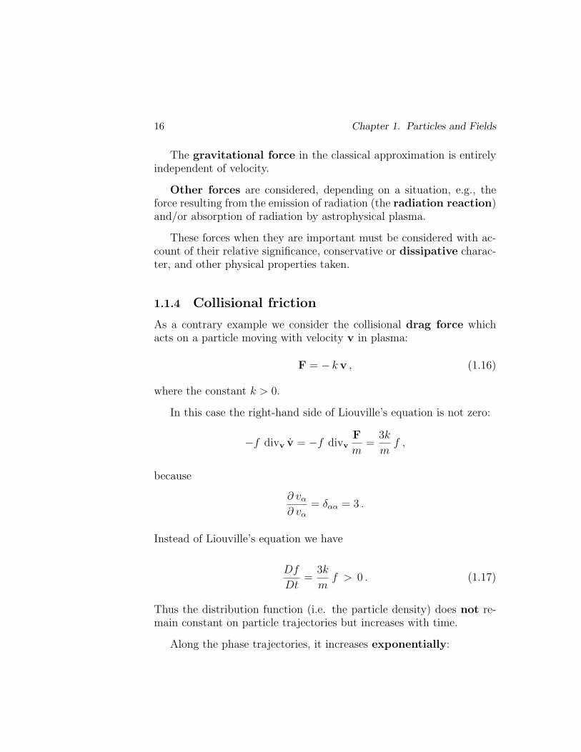
1.1.4 Collisional friction
As a contrary example we consider the collisional drag force whichacts on a particle moving with velocity v in plasma:
F = − k v , (1.16)
where the constant k > 0.
In this case the right-hand side of Liouville’s equation is not zero:
−f divv v = −f divvF
m=
3k
mf ,
because
∂ vα
∂ vα
= δαα = 3 .
Instead of Liouville’s equation we have
Df
Dt=
3k
mf > 0 . (1.17)
Thus the distribution function (i.e. the particle density) does not re-main constant on particle trajectories but increases with time.
Along the phase trajectories, it increases exponentially:
1.1. Liouville’s Theorem 17
f(t, r,v) ∼ f(0, r,v) exp
(3k
mt
). (1.18)
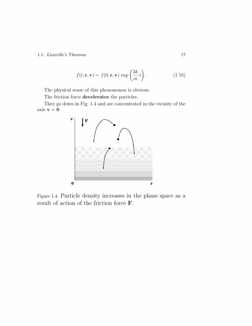
The physical sense of this phenomenon is obvious.
The friction force decelerates the particles.
They go down in Fig. 1.4 and are concentrated in the vicinity of theaxis v = 0.
v
r0
F
Figure 1.4: Particle density increases in the phase space as aresult of action of the friction force F.
18 Chapter 1. Particles and Fields
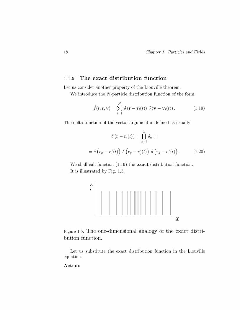
1.1.5 The exact distribution function
Let us consider another property of the Liouville theorem.
We introduce the N -particle distribution function of the form
f(t, r,v) =N∑
i=1
δ (r− ri(t)) δ (v − vi(t)) . (1.19)
The delta function of the vector-argument is defined as usually:
δ (r− ri(t)) =3∏
α=1
δα =
= δ(rx − r i
x(t))
δ(ry − r i
y(t))
δ(rz − r i
z(t)). (1.20)
We shall call function (1.19) the exact distribution function.
It is illustrated by Fig. 1.5.
X
f
<
Figure 1.5: The one-dimensional analogy of the exact distri-bution function.
Let us substitute the exact distribution function in the Liouvilleequation.
Action:
1.1.5. Exact Distribution Function 19
∂
∂t+ v · ∇r +
F
m· ∇v ==> f ==> = 0 .
The resulting three terms are
∂f
∂t=
∑
i
(−1) δ ′α (r− ri(t)) r iα δ (v − vi(t)) +
+∑
i
(−1) δ (r− ri(t)) δ ′α (v − vi(t)) v iα , (1.21)
v · ∇r f ≡ vα∂f
∂rα
=
=∑
i
vα δ ′α (r− ri(t)) δ (v − vi(t)) , (1.22)
F
m· ∇v f ≡ Fα
m
∂f
∂vα
=
=∑
i
Fα
mi
δ (r− ri(t)) δ ′α (v − vi(t)) . (1.23)
Here the index α = 1, 2, 3 or (x, y, z).
The prime denotes the derivative with respect to the argument ofa function.
The overdot denotes differentiation with respect to time t.
Summation over the repeated index α (contraction) is implied:
δ ′α r iα = δ ′x r i
x + δ ′y r iy + δ ′z r i
z .
The sum of terms (1.21)–(1.23) equals zero.
Let us rewrite it as follows
20 Chapter 1. Particles and Fields
0 =∑
i
(−r i
α + v iα
)δ ′α (r− ri(t)) δ (v − vi(t)) +
+∑
i
(−v i
α +Fα
mi
)δ (r− ri(t)) δ ′α (v − vi(t)) .
This can occur just then that all the coefficients of different combi-nations of delta functions with their derivatives equal zero as well.
Therefore we find
d r iα
dt= v i
α(t) ,d v i
α
dt=
1
mi
Fα (ri(t),vi(t)) . (1.24)
Thus
the Liouville equation for an exact distribution function isequivalent to the Newton set of equations for a particle mo-tion, both describing a purely dynamic behavior of the par-ticles.
It is natural since this distribution function is exact.
No statistical averaging has been done so far.
Statistics will appear later on when, instead of the exact descrip-tion of a system, we begin to use some mean characteristics such astemperature, density etc.
The statistical description is valid for systems containing a largenumber of particles.
We have shown that finding a solution of the Liouville equationfor an exact distribution function
1.1.5. Exact Distribution Function 21
Df
Dt= 0
(1.25)
is the same as the integration of the motion equations.
22 Chapter 1. Particles and Fields
However
for systems of a large number of interacting particles, it ismuch more advantageous to deal with the single Liouvilleequation for the exact distribution function which describesthe entire system.
1.2 Charged particles in the electromagnetic field
1.2.1 General formulation of the problem
Let us recall the basic physics notations and establish a common basis.
Maxwell’s equations for the electric field E and magnetic field Bare well known to have the form:
rot B =4π
cj +
1
c
∂ E
∂t, (1.26)
rot E = −1
c
∂ B
∂t, (1.27)
div B = 0 , (1.28)
div E = 4πρ q . (1.29)
The fields are completely determined by electric charges andelectric currents.
Note that Maxwell’s equations imply:
• the continuity equation for electric charge (see Exercise 1.5)
• the conservation law for electromagnetic field energy (Exer-cise 1.6).

1.2. Initial Equations 23
e1
0
ei
ri(t)vi(t)
eNq
tt
t
©©©©©©©©©* PPPqt
t
t
t
Figure 1.6: A system of N charged particles.
Let there be N particles with charges e1, e2, . . . ei, . . . eN, coordi-
nates ri(t) and velocities vi(t), see Fig. 1.6.
By definition, the electric charge density
ρ q (r, t) =N∑
i=1
ei δ (r− ri(t)) (1.30)
and the density of electric current
j (r, t) =N∑
i=1
ei vi(t) δ (r− ri(t)) . (1.31)
The coordinates and velocities of particles can be found by integrat-ing the equations of motion – the Newton equations:
ri = vi(t) , (1.32)
vi =1
mi
ei
[E (ri(t)) +
1
cvi ×B (ri(t))
]. (1.33)
Let us count the number of unknown quantities: the vectorsB, E, ri, and vi.
We obtain: 3 + 3 + 3N + 3N = 6 (N + 1).
The number of equations = 8 + 6N = 6 (N + 1) + 2.
24 Chapter 1. Particles and Fields
Therefore two equations seem to be unnecessary. Why is thisso?
1.2.2 The continuity equation for electric charge
At first let us make sure that the definitions (1.30) and (1.31) conformto the conservation law for electric charge.
Differentiating (1.30) with respect to time gives
∂ρ q
∂t= −∑
i
ei δ′α r i
α . (1.34)
Here the index α = 1, 2, 3.The prime denotes the derivative with respect to the argument of
the delta function.The overdot denotes differentiation with respect to time t.
For the electric current density (1.31) we have the divergence
div j =∂
∂rα
jα =∑
i
ei viα δ ′α . (1.35)
Comparing (1.34) with (1.35) we see that
∂ρ q
∂t+ div j = 0 .
(1.36)
Therefore the definitions for ρ q and j conform to the continuityequation.
As we shall see it in Exercise 1.5, conservation of electric chargefollows also directly from the Maxwell equations.
The difference is that above we have not used scalar Equation (1.29).
1.2. Initial Equations 25
1.2.3 Initial equations and initial conditions
Operating with the divergence on Equation (1.26)
Action:
div ==> rot B =4π
cj +
1
c
∂ E
∂t,
and using the continuity Equation (1.36),
Action:
div j = − ∂ρ q
∂t.
we obtain
0 =4π
c
(−∂ρ q
∂t
)+
1
c
∂
∂tdiv E .
Thus, we find that
∂
∂t( div E− 4πρ q ) = 0 . (1.37)
Hence Equation (1.29) will be valid at any moment of time, pro-vided it is true at the initial moment.
Let us operate with the divergence on Equation (1.27):
Action:
div ==> rot E = −1
c
∂ B
∂t,
∂
∂tdiv B = 0 . (1.38)
Equation (1.28) implies the absence of magnetic charges or, which isthe same, the solenoidal character of the magnetic field.
Conclusion. Equations (1.28) and (1.29) play the role of initialconditions for the time-dependent equations
26 Chapter 1. Particles and Fields
∂
∂tB = − c rot E (1.39)
and∂
∂tE = + c rot B− 4π j . (1.40)
Thus, in order to describe the gas consisting of N charged parti-cles, we consider the time-dependent problem of N bodies with a giveninteraction law.
The electromagnetic part of interaction is described by Max-well’s equations, the time-independent scalar equationsplaying the role of initial conditions for the time-dependent problem.
Therefore the set consisting of eight Maxwell’s equations and 6NNewton’s equations is neither over- nor under-determined.
It is closed with respect to the time-dependent problem, i.e. itconsists of 6 (N + 1) equations for 6 (N + 1) variables, once the initialand boundary conditions are given.
1.2.4 Astrophysical plasma applications
The set of equations described above can be treated analytically in justthree cases:
1. N = 1 , the motion of a charged particle in a given electro-magnetic field, e.g., drift motions and adiabatic invariants, wave-particle interaction, particle acceleration in astrophysical plasma.
2. N = 2 , Coulomb collisions of two charged particles, i.e. binarycollisions.
1.2. Initial Equations 27
This is important for the kinetic description of physical processes,e.g., the kinetic effects under propagation of accelerated parti-cles in plasma, collisional heating of plasma by a beam of fastelectrons or/and ions.
3. N → ∞ , a very large number of particles.
This case is the frequently considered one in plasma astrophysics,because it allows us to introduce macroscopic descriptions ofplasma, the widely-used magnetohydrodynamic (MHD) approxi-mation.
Intermediate case:
Numerical integration of Equations (1.26)–(1.33) in the case of largebut finite N , like N ≈ 3×10⁶, is possible by using modern computers.
The computations called particle simulations are increasinglyuseful for understanding many properties of astrophysical plasma andfor demonstration of them.
One important example of a simulation is magnetic reconnectionin a collisionless plasma.
This process often leads to fast energy conversion from field energyto particle energy, flares in astrophysical plasma (see Part II).
28 Chapter 1. Particles and Fields
Generalizations:
The set of equations described can be generalized to include consid-eration of neutral particles.
This is necessary, for instance, in the study of the generalizedOhm’s law which is applied in the investigation of physical processesin weakly-ionized plasmas, e.g., in the solar photosphere and pro-minences.
Dusty and self-gravitational plasmas in space are interesting inview of the diverse and often surprising facts about planetary ringsand comet environments, interstellar dark space.
1.3 Gravitational systems
Gravity plays a central role in the dynamics of many astrophysicalsystems – from stars to the Universe as a whole.
A gravitational force acts on the particles as follows:
mi vi = −mi∇φ . (1.41)
Here the gravitational potential
φ(t, r) = −N∑
n=1
G mn
| rn(t)− r | , n 6= i , (1.42)
G is the gravitational constant.
We shall return to this subject many times, e.g., while studying thevirial theorem.
This theorem is widely used in astrophysics.
Though the potential (1.42) looks similar to the Coulomb potentialof charged particles,
physical properties of gravitational systems differ so muchfrom properties of astrophysical plasma.
1.4. Practice: Exercises and Answers 29
We shall see this fundamental difference in what follows.
1.4 Practice: Exercises and Answers
Exercise 1.1. Show that
any distribution function that is a function of the constantsof motion – the invariants of motion – satisfies Liouville’sequation.
Answer.A general solution of the equations of motion (1.24) depends on 6N
constants Ci where i = 1, 2, ... 6N .
If the distribution function is a function of these constants of themotion
f = f ( C1, ... Ci, ... C6N ) , (1.43)
we rewrite the left-hand side of Equation (1.13) as
Df
Dt=
6N∑
i=1
(DCi
Dt
) (∂f
∂Ci
). (1.44)
Because Ci are constants of the motion, DCi/Dt = 0.
Therefore the right-hand side of Equation (1.44) is also zero. Q.e.d.
This is the so-called Jeans theorem.
Exercise 1.2. Rewrite the Liouville theorem by using the Hamiltonequations.
Answer.
Rewrite the Newton set of equations (1.24) in the Hamilton form:
qα =∂H
∂Pα
, Pα = −∂H
∂qα
, α = 1, 2, 3 . (1.45)
30 Chapter 1. Particles and Fields
Here H(P, q) is the Hamiltonian of a system, qα and Pα are the gen-eralized coordinates and momenta, respectively.
Let us substitute the variables r and v in the Liouville equation bythe generalized variables q and P:
∂f
∂t+∇P H · ∇q f −∇q H · ∇P f = 0 . (1.46)
Recall that the Poisson brackets for arbitrary quantities A and Bare defined to be
[ A , B ] =3∑
α=1
(∂A
∂qα
∂B
∂Pα
− ∂A
∂Pα
∂B
∂qα
). (1.47)
Applying (1.47) to (1.46), we find the final form of the Liouvilletheorem
∂f
∂t+ [ f , H ] = 0 .
(1.48)
Note that for a system in equilibrium
[ f , H ] = 0 . (1.49)
Exercise 1.3. Discuss what to do with the Liouville theorem, if itis impossible to disregard quantum indeterminacy and assume thatthe classical description of a system is justified.
Consider the case of dense fluids inside stars, for example, whitedwarfs.
Comment.
Inside a white dwarf star the temperature T ∼ 105 K, but thedensity is very high: n ∼ 1028 − 1030 cm−3.
The electrons cannot be regarded as classical particles.
1.4. Practice: Exercises and Answers 31
We have to consider them as a quantum system with a Fermi-Diracdistribution.
Exercise 1.4. Recall the Liouville theorem in a course of mechanics– the phase volume of a system is independent of t.
Show that this formulation is equivalent to Equation (1.13).
Exercise 1.5. Show that Maxwell’s equations imply the continuityequation for electric charge.
Answer.
Operating with the divergence on Equation (1.26),
Action:
div ==> rot B =4π
cj +
1
c
∂ E
∂t,
we have
0 =4π
cdiv j +
1
c
∂
∂tdiv E .
Substituting (1.29)
Comment:(1.29) : div E = 4πρ q ,
in this equation gives us the continuity equation for the electric charge
∂
∂tρ q + div j = 0 . (1.50)
Exercise 1.6. Starting from Maxwell’s equations, derive the energyconservation law for an electromagnetic field.
Answer.
Multiply Equation (1.26) by the electric field vector E and add itto Equation (1.27) multiplied by the magnetic field vector B.
The result is
32 Chapter 1. Particles and Fields
∂
∂tW = − j E− div G .
(1.51)
Here
W =E2 + B2
8π(1.52)
is the energy of electromagnetic field in a unit volume of space;
G =c
4π[E×B ] (1.53)
is the flux of electromagnetic field energy through a unit surface inspace, i.e. the Poynting vector.
The first term on the right-hand side of Equation (1.51) is the powerof work done by the electric field on all the charged particles in the unitvolume of space.
In the simplest approximation
evE =d
dtE , (1.54)
where E is the particle kinetic energy.
Hence instead of Equation (1.51) we write the following form of theenergy conservation law:
∂
∂t
(E2 + B2
8π+
ρv2
2
)+ div
(c
4π[E×B ]
)= 0 . (1.55)
Chapter 2
Statistical Description ofInteracting Particle Systems
In a system which consists of many interacting particles, thestatistical mechanism of ‘mixing’ in phase space works andmakes the system’s behavior on average more simple.
2.1 The averaging of Liouville’s equation
2.1.1 Averaging over phase space
As was shown above, the exact state of a system consisting of N in-teracting particles can be given by the exact distribution function inthe 6D phase space X = r,v.
This function is the sum of δ-functions in N points of the phasespace:
f(r,v, t) =N∑
i=1
δ (r− ri(t)) δ (v − vi(t)) . (2.1)
We use Liouville’s equation to describe the change of the systemstate:
∂f
∂t+ v · ∇r f +
F
m· ∇v f = 0 . (2.2)
33
34 Chapter 2. Statistical Description
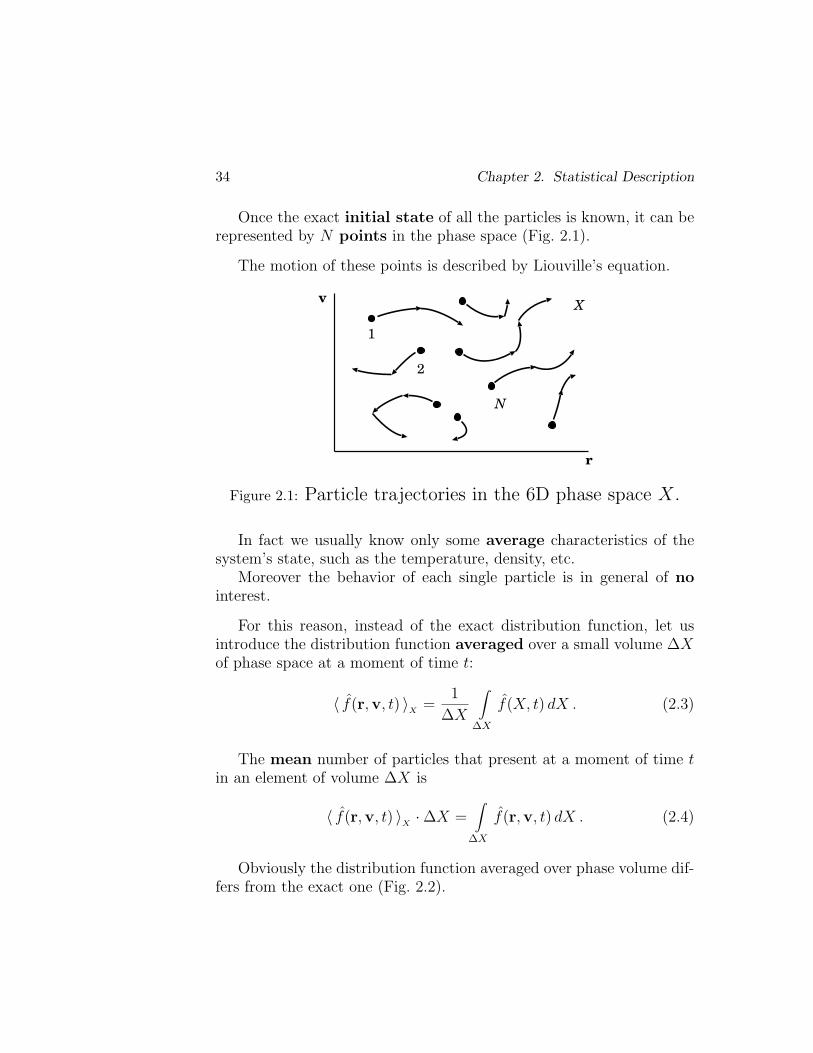
Once the exact initial state of all the particles is known, it can berepresented by N points in the phase space (Fig. 2.1).
The motion of these points is described by Liouville’s equation.
v
r
X
1
2
N
Figure 2.1: Particle trajectories in the 6D phase space X.
In fact we usually know only some average characteristics of thesystem’s state, such as the temperature, density, etc.
Moreover the behavior of each single particle is in general of nointerest.
For this reason, instead of the exact distribution function, let usintroduce the distribution function averaged over a small volume ∆Xof phase space at a moment of time t:
〈 f(r,v, t) 〉X
=1
∆X
∫
∆X
f(X, t) dX . (2.3)
The mean number of particles that present at a moment of time tin an element of volume ∆X is
〈 f(r,v, t) 〉X·∆X =
∫
∆X
f(r,v, t) dX . (2.4)
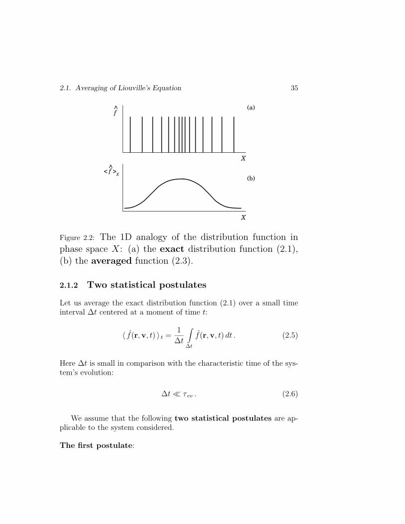
Obviously the distribution function averaged over phase volume dif-fers from the exact one (Fig. 2.2).
2.1. Averaging of Liouville’s Equation 35
X
X
f
f
X<
<
>
<
(a)
(b)
Figure 2.2: The 1D analogy of the distribution function inphase space X: (a) the exact distribution function (2.1),(b) the averaged function (2.3).
2.1.2 Two statistical postulates
Let us average the exact distribution function (2.1) over a small timeinterval ∆t centered at a moment of time t:
〈 f(r,v, t) 〉 t =1
∆t
∫
∆t
f(r,v, t) dt . (2.5)
Here ∆t is small in comparison with the characteristic time of the sys-tem’s evolution:
∆t ¿ τ ev . (2.6)
We assume that the following two statistical postulates are ap-plicable to the system considered.
The first postulate:
36 Chapter 2. Statistical Description
The mean values 〈 f 〉X
and 〈 f 〉 t exist for sufficiently small∆X and ∆t and are independent of the averaging scales ∆Xand ∆t.
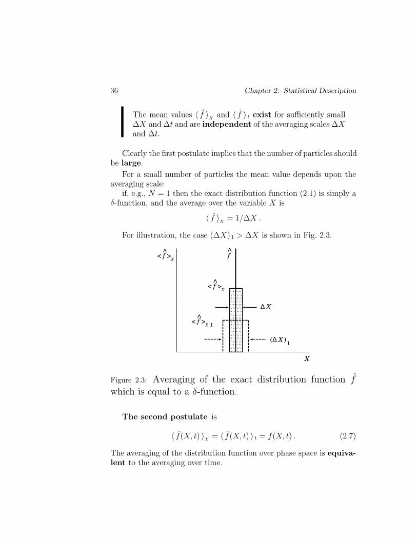
Clearly the first postulate implies that the number of particles shouldbe large.
For a small number of particles the mean value depends upon theaveraging scale:
if, e.g., N = 1 then the exact distribution function (2.1) is simply aδ-function, and the average over the variable X is
〈 f 〉X
= 1/∆X .
For illustration, the case (∆X) 1 > ∆X is shown in Fig. 2.3.
X
X
f
f
X<
<
>
<
fX
<<
>
∆
X∆( )1
fX
<
<
>1
Figure 2.3: Averaging of the exact distribution function f
which is equal to a δ-function.
The second postulate is
〈 f(X, t) 〉X
= 〈 f(X, t) 〉 t = f(X, t) . (2.7)
The averaging of the distribution function over phase space is equiva-lent to the averaging over time.
2.1. Averaging of Liouville’s Equation 37
While speaking of the small ∆X and ∆t, we assume that they arenot too small:
∆X must contain a reasonably large number of particles while
∆t must be large in comparison with the duration of drastic changesof the exact distribution function, such as the duration of the particlecollisions:
∆t À τc . (2.8)
It is in this case that the statistical mechanism of particle ‘mixing’in phase space is at work and
the averaging of the exact distribution function over thetime ∆t is equivalent to the averaging over the phase vol-ume ∆X.
2.1.3 A statistical mechanism of mixing
Let us try to understand qualitatively how the mixing mechanismworks in phase space.
We start from the dynamical description of the N -particle systemin 6N -dimensional phase space in which
Γ = ri, vi , i = 1, 2, . . . N, (2.9)
a point is determined (t = 0 in Fig. 2.4) by the initial conditions of allthe particles.
The motion of this point is described by Liouville’s equation.
The point moves along a complicated dynamical trajectory be-cause the interactions in a many-particle system are extremely intricateand complicated.
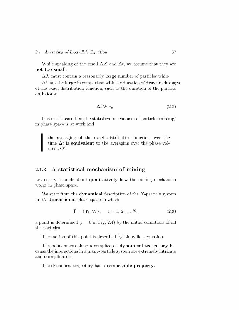
The dynamical trajectory has a remarkable property.
38 Chapter 2. Statistical Description
v
ri
i
t = 0
∆
Γ
Γ
1023
Figure 2.4: The dynamical trajectory of a system of N parti-cles in the 6N -D phase space Γ.
Imagine a glass vessel containing a gas consisting of a large num-ber N of particles.
The state of this gas at any moment of time is depicted by a singlepoint in the phase space Γ.
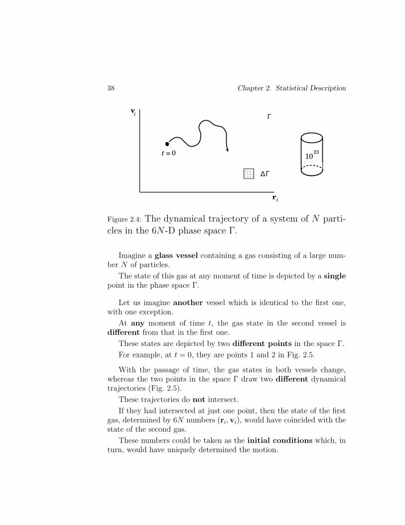
Let us imagine another vessel which is identical to the first one,with one exception.
At any moment of time t, the gas state in the second vessel isdifferent from that in the first one.
These states are depicted by two different points in the space Γ.
For example, at t = 0, they are points 1 and 2 in Fig. 2.5.
With the passage of time, the gas states in both vessels change,whereas the two points in the space Γ draw two different dynamicaltrajectories (Fig. 2.5).
These trajectories do not intersect.
If they had intersected at just one point, then the state of the firstgas, determined by 6N numbers (ri,vi), would have coincided with thestate of the second gas.
These numbers could be taken as the initial conditions which, inturn, would have uniquely determined the motion.
2.1. Averaging of Liouville’s Equation 39
v
ri
i
t = 0
∆
Γ
Γ
1
2
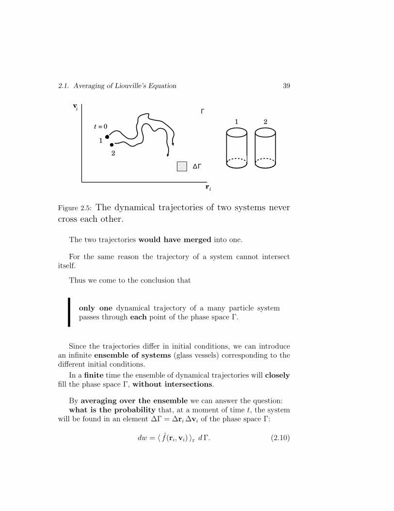
1 2
Figure 2.5: The dynamical trajectories of two systems nevercross each other.
The two trajectories would have merged into one.
For the same reason the trajectory of a system cannot intersectitself.
Thus we come to the conclusion that
only one dynamical trajectory of a many particle systempasses through each point of the phase space Γ.
Since the trajectories differ in initial conditions, we can introducean infinite ensemble of systems (glass vessels) corresponding to thedifferent initial conditions.
In a finite time the ensemble of dynamical trajectories will closelyfill the phase space Γ, without intersections.
By averaging over the ensemble we can answer the question:what is the probability that, at a moment of time t, the system
will be found in an element ∆Γ = ∆ri ∆vi of the phase space Γ:
dw = 〈 f(ri,vi) 〉Γ d Γ. (2.10)
40 Chapter 2. Statistical Description
Here 〈 f(ri,vi) 〉Γ is a function of all the coordinates and velocities.
It plays the role of the probability distribution density in thephase space Γ and is called the statistical distribution function or simplythe distribution function.
∗ ∗ ∗
It is obvious that the same probability density can be obtainedin another way – through the averaging over time.
The dynamical trajectory of a system, given a sufficient large time ∆t,will closely cover the space Γ.
Since the trajectory is very intricate, it will repeatedly pass throughthe phase space element ∆Γ.
Let (∆t)Γ
be the time during which the system locates in ∆Γ.
For a sufficiently large ∆t, which is formally restricted by the char-acteristic time of evolution of the system as a whole, the ratio (∆t)
Γ/∆t
tends to the limit
lim∆t→∞
( ∆t )Γ
∆t=
dw
d Γ= 〈 f(ri,vi, t) 〉 t . (2.11)
By virtue of the role of the probability density, it is clear that
the statistical averaging over the ensemble (2.10) is equiva-lent to the averaging over time (2.11) as well as to the defini-tion (2.5).
2.1.4 Derivation of a general kinetic equation
Now we have everything what we need to average the exact Liouvilleequation
∂f
∂t+ v · ∇r f +
F
m· ∇v f = 0 .
2.1. Averaging of Liouville’s Equation 41
Since the equation contains the derivatives with respect to time tand phase-space coordinates (r,v), the procedure of averaging is definedas follows:
f(X, t) =1
∆X ∆t
∫
∆X
∫
∆t
f(X, t) dX dt . (2.12)
Averaging the first term of the Liouville equation gives
1
∆X ∆t
∫
∆X
∫
∆t
∂f
∂tdX dt =
1
∆t
∫
∆t
∂
∂t
1
∆X
∫
∆X
f dX
dt =
=1
∆t
∫
∆t
∂
∂tf dt =
∂f
∂t. (2.13)
In the last equality the use is made of the fact that, by virtue of thesecond postulate, the averaging of a smooth averaged function does notchange it.
Let us average the second term in Equation (2.2):
1
∆X ∆t
∫
∆X
∫
∆t
vα∂f
∂rα
dX dt =
=1
∆X
∫
∆X
vα∂
∂rα
1
∆t
∫
∆t
f dt
dX =
=1
∆X
∫
∆X
vα∂
∂rα
f dX = vα∂f
∂rα
. (2.14)
Here the index α = 1, 2, 3.
To average the term containing the force F, let us represent it as asum of a mean force 〈F 〉 and the force due to the difference of thereal force field from the mean (smooth) one:
42 Chapter 2. Statistical Description
F = 〈F 〉+ F ′. (2.15)
Substituting (2.15) in the third term in Equation (2.2) and averagingit, we have
1
∆X ∆t
∫
∆X
∫
∆t
Fα
m
∂f
∂vα
dX dt =
=〈Fα 〉
m
1
∆X
∫
∆X
∂
∂vα
1
∆t
∫
∆t
f dt
dX+
+1
∆X ∆t
∫
∆X
∫
∆t
F ′α
m
∂f
∂vα
dX dt =
=〈Fα 〉
m
∂f
∂vα
+1
∆X ∆t
∫
∆X
∫
∆t
F ′α
m
∂f
∂vα
dX dt . (2.16)
Gathering all three terms together, we write the averaged Liouvilleequation in the form
∂f
∂t+ v · ∇r f +
〈F 〉m
· ∇v f =
(∂f
∂t
)
c
,
(2.17)
where
(∂f
∂t
)
c
= − 1
∆X ∆t
∫
∆X
∫
∆t
F ′α
m
∂f
∂vα
dX dt .
(2.18)
2.2. Collisional Integral 43
Equation (2.17) and its right-hand side (2.18) are called the kineticequation and the collisional integral, respectively.
Thus we have found the most general form of the kinetic equa-tion with a collisional integral, which cannot be directly used in plasmaastrophysics, without making some additional simplifying assump-tions.
The main of them is the binary character of collisions.
2.2 A collisional integral and correlation functions
2.2.1 Binary interactions
The statistical mechanism of mixing in phase space makes particleshave no individuality.
However, we have to distinguish different kinds of particles, e.g.,electrons and protons, because their behaviors differ.
Let fk (r,v, t) be the exact distribution function of particles of thekind k
fk (r,v, t) =Nk∑
i=1
δ (r− rki(t)) δ (v − vki(t)) , (2.19)
the index i denoting the ith particle of kind k, Nk being the number ofparticles of kind k.
The Liouville equation for the particles of kind k takes a view
∂fk
∂t+ v · ∇r fk +
Fk
mk
· ∇v fk = 0 , (2.20)
mk is the mass of a particle of kind k.
The force acting on a particle of kind k at a point (r,v) of the phase
space X at a moment of time t, Fk,α (r,v, t), is the sum of forces actingon this particle from all other particles (Fig. 2.6):
44 Chapter 2. Statistical Description
F k,α (r,v, t) =∑
l
Nl∑
i=1
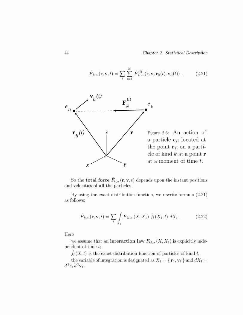
F(i)kl,α (r,v, rli(t),vli(t)) . (2.21)
r
Fkl
rli
(t)
eli
ek
x y
z
(i)v
li(t)
Figure 2.6: An action ofa particle e li located atthe point r li on a parti-cle of kind k at a point rat a moment of time t.
So the total force Fk,α (r,v, t) depends upon the instant positionsand velocities of all the particles.
By using the exact distribution function, we rewrite formula (2.21)as follows:
F k,α (r,v, t) =∑
l
∫
X1
F kl,α (X, X1) fl (X1, t) dX1 . (2.22)
Here
we assume that an interaction law Fkl,α (X, X1) is explicitly inde-pendent of time t;
fl (X, t) is the exact distribution function of particles of kind l,
the variable of integration is designated as X1 = r1,v1 and dX1 =d 3r1 d 3v1.
2.2. Collisional Integral 45
Formula (2.22) takes into account that the forces consideredare binary ones, i.e. they can be represented as a sum ofinteractions between two particles.
Making use of the representation (2.22), let us average the forceterm in the Liouville equation, as this has been done in formula (2.16).
We have
1
∆X ∆t
∫
∆X
∫
∆t
1
mk
F k,α (r,v, t)∂fk
∂vα
dX dt =
=1
∆X ∆t
∫
∆X
∫
∆t
∑
l
∫
X1
1
mk
F kl,α (X, X1) fl (X1, t)×
× ∂
∂vα
fk (X, t) dX dX1 dt =
=1
∆X
∫
∆X
∑
l
∫
X1
1
mk
F kl,α (X, X1) ×
× ∂
∂vα
1
∆t
∫
∆t
fk (X, t) fl (X1, t) dt
dX dX1 . (2.23)
Here we have taken into account that the exact distribution func-tion fl (X1, t) is independent of the velocity v, which is a part of thevariable X = r, v related to the particles of the kind k.
Formula (2.23) contains the pair products of exact distribu-tion functions of different particle kinds, as is natural for thecase of binary interactions.
46 Chapter 2. Statistical Description
2.2.2 Binary correlation
Let us represent the exact distribution function fk as
fk (X, t) = fk (X, t) + ϕk (X, t) , (2.24)
where
fk (X, t) is the statistically averaged distribution function,
ϕk (X, t) is the deviation of the exact distribution function from theaveraged one.
It is obvious that, according to (2.24),
ϕk (X, t) = fk (X, t)− fk (X, t) ;
hence
〈 ϕk (X, t) 〉 = 0 . (2.25)
Let us consider the integrals of pair products in the averagedforce term (2.23).
In view of definition (2.24), they can be rewritten as
1
∆t
∫
∆t
fk (X, t) fl (X1, t) dt =
= fk (X, t) fl (X1, t) + fkl (X, X1, t) , (2.26)
where
fkl (X,X1, t) =1
∆t
∫
∆t
ϕk (X, t) ϕl (X1, t) dt . (2.27)
The function fkl is referred to as the correlation function or, moreexactly, the binary correlation function.
The physical meaning of the correlation function is clear from (2.26).
2.2. Collisional Integral 47
The left-hand side of (2.26) means the probability to find a particleof kind k at a point X of the phase space at a moment of time t undercondition that a particle of kind l places at a point X1 at the sametime.
By definition this is a conditional probability.
In the right-hand side of (2.26) the distribution function fk (X, t)characterizes the probability that a particle of kind k stays at a point Xat a moment of time t.
The function fl (X1, t) plays the analogous role for the particles ofkind l.
If the particles of kind k did not interact with those of kind l,then their distributions would be independent, i.e. probabilitydensities would simply multiply:
〈 fk (X, t) fl (X1, t) 〉 = fk (X, t) fl (X1, t) . (2.28)
So in the right-hand side of (2.26) there should be
fkl (X,X1, t) = 0 . (2.29)
There would be no correlation in the particle distribution.
We consider a system of interacting particles.
With the proviso that the parameter characterizing the binary in-teraction, e.g., Coulomb collision considered below,
ζ i ≈ e2
〈 l 〉
/ ⟨mv2
2
⟩, (2.30)
is small under conditions in a wide range, the correlation function mustbe relatively small.
48 Chapter 2. Statistical Description
If the interaction is weak, the second term in the right-handside of (2.26) must be small in comparison with the first one.
This fundamental property allows us to construct a theory of plasmain many cases of astrophysical interest.
2.2.3 The collisional integral and binary correlation
Now let us substitute (2.26) in formula (2.23) for the averaged forceterm:
1
∆X ∆t
∫
∆X
∫
∆t
1
mk
F k,α (X, t)∂fk
∂vα
dX dt =
=1
∆X
∫
∆X
∑
l
∫
X1
1
mk
F kl,α (X, X1)∂
∂vα
[ fk (X, t) fl (X1, t) +
+ fkl (X, X1, t) ] dX dX1 =
since fk (X, t) is a smooth function, its derivative over vα can be broughtout of the averaging procedure:
=
[∂
∂vα
fk (X, t)
]×
×
1
∆X
∫
∆X
∑
l
∫
X1
1
mk
F kl,α (X,X1) fl (X1, t) dX dX1
+
+1
∆X
∫
∆X
∑
l
∫
X1
1
mk
F kl,α (X,X1)∂
∂vα
fkl (X, X1, t) dX dX1 =
2.2. Collisional Integral 49
=1
mk
F k,α (X, t)∂fk (X, t)
∂vα
+
+∑
l
∫
X1
1
mk
F kl,α (X, X1)∂fkl (X, X1, t)
∂vα
dX1 . (2.31)
Here we have taken into account that the averaging of smooth functionsdoes not change them, and the following definition of the averagedforce is used:
F k,α (X, t) =1
∆X
∫
∆X
∑
l
∫
X1
F kl,α (X,X1) fl (X1, t) dX dX1 =
=∑
l
∫
X1
F kl,α (X, X1) fl (X1, t) dX1 . (2.32)
This definition coincides with the previous definition (2.16) of the av-eraged force, since
all the deviations of the real force Fk from the mean (smooth)force Fk are taken care of in the deviations ϕk and ϕl of thereal distribution functions fk and fl from their mean values fk
and fl.
Thus the collisional integral is represented in the form
(∂fk
∂t
)
c
= −∑
l
∫
X1
1
mk
F kl,α (X, X1)∂fkl (X, X1, t)
∂vα
dX1 . (2.33)
Let us recall that for the Lorentz force as well as for the gravi-tational one the condition
∂
∂vα
F kl,α (X, X1) = 0 (2.34)
50 Chapter 2. Statistical Description
is satisfied.
So, we obtain from formula (2.33) the following expression
(∂fk
∂t
)
c
= − ∂
∂vα
∑
l
∫
X1
1
mk
F kl,α (X, X1) fkl (X,X1, t) dX1 . (2.35)
Hence the collisional integral can be written in the divergent formin the velocity space v :
(∂fk
∂t
)
c
= − ∂
∂vα
J k,α ,
(2.36)
where the flux of particles of kind k in the velocity space is
J k,α (X, t) =∑
l
∫
X1
1
mk
F kl,α (X, X1) fkl (X,X1, t) dX1 . (2.37)
Therefore the averaged Liouville equation or the kinetic equationfor particles of kind k
∂fk (X, t)
∂t+ vα
∂fk (X, t)
∂rα
+F k,α (X, t)
mk
∂fk (X, t)
∂vα
=
= − ∂
∂vα
∑
l
∫
X1
1
mk
F kl,α (X,X1) fkl (X, X1, t) dX1 (2.38)
contains the unknown function fkl.
Hence the kinetic Equation (2.38) for distribution function fk is notclosed.
We have to find the equation for the correlation function fkl .
2.3. Correlation Functions 51
2.3 Equations for correlation functions
To derive the equations for correlation functions, it is not necessary tointroduce any new postulates or develop new formalisms.
All the necessary equations and averaging procedures are at hand.
Looking at definition
fkl (X,X1, t) =1
∆t
∫
∆t
ϕk (X, t) ϕl (X1, t) dt ,
where
ϕk (X, t) = fk (X, t)− fk (X, t) ,
we see that we need an equation which will describe the deviation ofdistribution function from its mean value, i.e. the function ϕk = fk−fk.
In order to derive such equation, we simply have to subtract theaveraged Liouville equation
∂fk (X, t)
∂t+ vα
∂fk (X, t)
∂rα
+ ... = ...
from the exact Liouville equation (2.2)
∂fk
∂t+ v · ∇r fk +
Fk
mk
· ∇v fk = 0 .
The result is
∂ ϕk (X, t)
∂t+ vα
∂ ϕk (X, t)
∂rα
+F k,α
mk
∂fk
∂vα
− F k,α
mk
∂fk
∂vα
=
=∂
∂vα
∑
l
∫
X1
1
mk
F kl,α (X, X1) fkl (X,X1) dX1 . (2.39)
Here
52 Chapter 2. Statistical Description
F k,α (X, t) =∑
l
∫
X1
F kl,α (X, X1) fl (X1, t) dX1 (2.40)
is the exact force (2.22) acting on a particle of the kind k, and
F k,α (X, t) =∑
l
∫
X1
F kl,α (X,X1) fl (X1, t) dX1 (2.41)
is the statistically averaged force.
Considering that we need the equation for the pair correlation func-tion
fkl (X1, X2, t) = 〈 ϕk (X1, t) ϕl (X2, t) 〉 ,
let us take two equations:
one for ϕk (X1, t)
∂ ϕk (X1, t)
∂t+ v 1,α
∂ ϕk (X1, t)
∂ r1,α
+ . . . = 0 (2.42)
and another for ϕl (X2, t)
∂ ϕl (X2, t)
∂t+ v 2,α
∂ ϕl (X2, t)
∂ r2,α
+ . . . = 0 . (2.43)
Now we add the equations resulting from (2.42) multiplied by ϕl
and (2.43) multiplied by ϕk.
We obtain
ϕl∂ ϕk
∂t+ ϕk
∂ ϕl
∂t+ v 1,α
∂ ϕk
∂ r1,α
ϕl + . . . = 0
or
2.3. Correlation Functions 53
∂ (ϕk ϕl)
∂t+ v 1,α
∂ (ϕk ϕl)
∂ r1,α
+ v 2,α∂ (ϕk ϕl)
∂ r2,α
+ . . . = 0 . (2.44)
On averaging Equation (2.44) we have the equation for the paircorrelation function:
∂fkl (X1, X2, t)
∂t+
+ v 1,α∂fkl (X1, X2, t)
∂ r1,α
+ v 2,α∂fkl (X1, X2, t)
∂ r2,α
+
+F k,α (X1, t)
mk
∂fkl (X1, X2, t)
∂ v 1,α
+F l,α (X2, t)
ml
∂fkl (X1, X2, t)
∂ v 2,α
+
+∂fk (X1, t)
∂ v 1,α
∑n
∫
X3
1
mk
F kn,α (X1, X3) fnl (X3, X2, t) dX3 +
+∂fl (X2, t)
∂ v 2,α
∑n
∫
X3
1
ml
F ln,α (X2, X3) fnk (X3, X1, t) dX3 =
= − ∂
∂ v 1,α
∑n
∫
X3
1
mk
F kn,α (X1, X3) fkln (X1, X2, X3, t) dX3 −
− ∂
∂ v 2,α
∑n
∫
X3
1
ml
F ln,α (X2, X3) fkln (X1, X2, X3, t) dX3 . (2.45)
Here
fkln (X1, X2, X3, t) =1
∆t
∫
∆t
ϕk (X1, t) ϕl (X2, t) ϕn (X3, t) dt (2.46)
is the function of triple correlations.
Thus Equation (2.45) for the pair correlation function contains theunknown function of triple correlations.
54 Chapter 2. Statistical Description
In general,
the chain of equations for correlation functions is unclosed:the equation for the correlation function of sth order containsthe function of the order (s + 1).
2.4 Practice: Exercises and Answers
Exercise 2.1. By analogy with formula (2.26), show that
〈 fk (X1, t) fl (X2, t) fn (X3, t) 〉 = (2.47)
= fk (X1, t) fl (X2, t) fn (X3, t) +
+ fk (X1, t) fln (X2, X3, t) + fl (X2, t) fkn (X1, X3, t) +
+ fn (X3, t) fkl (X1, X2, t) + fkln (X1, X2, X3, t) .
Exercise 2.2. Discuss a similarity and difference between the kinetictheory presented in this Chapter and the famous BBGKY hierarchy the-ory developed by Bogoliubov, Born and Green, Kirkwood, and Yvon.
Hint. Show that essential to both derivations is the weak-couplingassumption, according to which
grazing encounters, involving small fractional energy and mo-mentum exchange between colliding particles, dominate theevolution of the velocity distribution function.
The weak-coupling assumption provides justification of the widelyappreciated practice which leads to a very significant simplification ofthe original collisional integral.
Chapter 3
Weakly-Coupled Systemswith Binary Collisions
In a system of many interacting particles, the weak-couplingassumption allows us to introduce a well controlled ap-proximation to consider the chain of the equations for cor-relation functions.
This leads to a significant simplification of the collisionalintegral in astrophysical plasma but not in self-gravitatingsystems.
3.1 Approximations for binary collisions
3.1.1 The small parameter of kinetic theory
The infinite chain of equations for the correlation functions does notcontain more information in itself than the Liouville equation for theexact distribution function.
Actually, the statistical smoothing allows to lose ‘useless informa-tion’ – the information about the exact motion of particles.
The value of the chain is that it allows a direct introduction ofnew physical assumptions which make it possible to break the chainoff at some term (Fig. 3.1) and to estimate the resulting error.
55
56 Chapter 3. Weakly-Coupled Systems
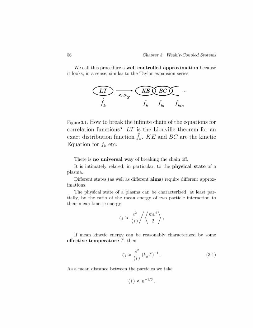
We call this procedure a well controlled approximation becauseit looks, in a sense, similar to the Taylor expansion series.
LT KE
fk
fk
fkl
< >X
fkln
...BC
Figure 3.1: How to break the infinite chain of the equations forcorrelation functions? LT is the Liouville theorem for anexact distribution function fk. KE and BC are the kineticEquation for fk etc.
There is no universal way of breaking the chain off.
It is intimately related, in particular, to the physical state of aplasma.
Different states (as well as different aims) require different approx-imations.
The physical state of a plasma can be characterized, at least par-tially, by the ratio of the mean energy of two particle interaction totheir mean kinetic energy
ζ i ≈ e2
〈 l 〉
/ ⟨mv2
2
⟩,
If mean kinetic energy can be reasonably characterized by someeffective temperature T , then
ζ i ≈ e2
〈 l 〉 (kBT )−1 . (3.1)
As a mean distance between the particles we take
〈 l 〉 ≈ n−1/3 .

3.1. Binary Collisions 57
Hence
ζ i =e2
kB
× n1/3
T(3.2)
is termed the interaction parameter.
It is small for a sufficiently hot and rarefied plasma.
In many astrophysical plasmas, e.g., in the solar corona, the in-teraction parameter is very small.
So
the thermal kinetic energy of plasma particles is much largerthan their interaction energy.
The particles are almost free or moving on definite trajectories inthe external fields if the later are present.
We call this case the approximation of weak Coulomb interaction.
While constructing a kinetic theory, it is natural to use the pertur-bation procedure with respect to the small parameter ζ i.
This means that
the distribution function fk must be taken to be of order unity,the pair correlation function fkl of order ζ i, the triple corre-lation function fkln of order ζ 2
i , etc.
We shall see in what follows that this principle has a deep physicalsense in kinetic theory.
Such plasmas are said to be ‘weakly coupled’.
An opposite case, when the interaction parameter takes values largerthan unity, is dense, relatively cold plasmas, for example in the inte-riors of white dwarf stars.
These plasmas are ‘strongly coupled’.
58 Chapter 3. Weakly-Coupled Systems
3.1.2 The Vlasov kinetic equation
In the zeroth order with respect to the small parameter ζ i, we obtain theVlasov equation with the self-consistent electromagnetic field:
∂fk (X, t)
∂t+ vα
∂fk (X, t)
∂rα
+
+ek
mk
(E +
1
cv ×B
)
α
∂fk (X, t)
∂vα
= 0 . (3.3)
Here E and B are the statistically averaged electric and magneticfields obeying Maxwell’s equations:
curl E = −1
c
∂ B
∂t, div E = 4π ( ρ 0 + ρ q ) ,
(3.4)
curl B =1
c
∂ E
∂t+
4π
c( j 0 + j q ) , div B = 0 .
ρ 0 and j 0 are the external charges and currents; they describe theexternal fields, e.g., the uniform magnetic field B0.
ρ q and j q are the statistically smoothed charge and current due tothe plasma particles:
ρ q (r, t) =∑
k
ek
∫
v
fk (r,v, t) d 3v , (3.5)
j q (r, t) =∑
k
ek
∫
v
v fk (r,v, t) d 3v . (3.6)
Therefore the electric and magnetic fields are also statistically smoothed.
If we are considering processes which occur on a time scale muchshorter than the time of collisions,
3.1. Binary Collisions 59
τ ev ¿ τc , (3.7)
we use a description which includes the averaged electric and mag-netic fields but neglects the microfields responsible for binarycollisions.
This means thatF ′ = 0 ,
therefore the collisional integral is also equal to zero.
The Vlasov equation together with the definitions (3.5) and (3.6),and with Maxwell’s Equations (3.4) is a nonlinear integro-differentialequation.
It serves as a classic basis for the theory of oscillations and wavesin a plasma with the small parameter ζ i .
The Vlasov equation is also a proper basis for theory of wave-particle interactions in astrophysical plasma and collisionless shockwaves, collisionless reconnecting current layers.
3.1.3 The Landau collisional integral
Using the perturbation procedure with respect to the small parame-ter ζ i in the first order, and neglecting the close Coulomb collisions,we find the kinetic equation with the collisional integral given by Lan-dau
(∂fk
∂t
)
c
= − ∂
∂vα
J k,α , (3.8)
Here the flux of particles of kind k in the velocity space is
J k,α =πe 2
k ln Λ
mk
∑
l
e 2l
∫
vl
fk
∂fl
ml ∂ v l,β
− fl∂fk
mk ∂ v k,β
×
× (u2 δαβ − uαuβ)
u3d 3vl . (3.9)
60 Chapter 3. Weakly-Coupled Systems
u = v − vl is the relative velocity, d 3vl corresponds to the integrationover the whole velocity space of ‘field’ particles l.
ln Λ is the Coulomb logarithm which takes into account divergenceof the Coulomb-collision cross-section.
The kinetic equation with the Landau integral is a nonlinear integro-differential equation for the distribution function fk (r,v, t).
Two approaches correspond to different limiting cases.
The Landau integral takes into account the part of the particleinteraction which determines dissipation while the Vlasovequation allows for the averaged field, and is thus reversible.
For example, in the Vlasov theory, the question of the role of colli-sions in the neighbourhood of resonances remains open.
The famous paper by Landau (1946) was devoted to this problem.
Landau used the reversible Vlasov equation as the basis to study thedynamics of a small perturbation of the Maxwell distribution function,f (1)(r,v, t).
In order to solve the linearized Vlasov equation, he made use of theLaplace transformation, and defined the rule to avoid a pole at
ω = k‖ v‖
in the divergent integral by the replacement
ω → ω + i 0 .
This technique for avoiding singularities may be formally replacedby a different procedure.
Namely it is possible to add a small dissipative term−νf (1)(r,v, t)to the right-hand side of the linearized Vlasov equation.
In this way, the Fourier transform of the kinetic equation involvesthe complex frequency
ω = ω′ + i ν ,
3.1. Binary Collisions 61
leading with ν → 0 to the same expression for the Landau damping.
Note, however, that
the Landau damping is not by collisions but by a transfer ofwave field energy into oscillations of resonant particles.
The Landau method is really a beautiful example of complex anal-ysis leading to an important new physical result.
The second approach reduces the reversible Vlasov equation to anirreversible one.
Although the dissipation is assumed to be negligibly small, one can-not take the limit ν → 0 directly in the master equations: this can bedone only in the final formulae.
This method of introducing a collisional damping is natural.
It shows that
even very rare collisions play the principal role in the physicsof collisionless plasma.
3.1.4 The Fokker-Planck equation
The smallness of the interaction parameter signifies that, in the col-lisional integral, the sufficiently distant Coulomb collisions are takencare of as the interactions with a small momentum and energytransfer.
For this reason, it comes as no surprise that the Landau integralcan be considered as a particular case of a different approach which isthe Fokker-Planck equation.
Let us consider a distribution function independent of space sothat f = f(v, t).
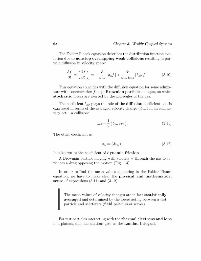
62 Chapter 3. Weakly-Coupled Systems
The Fokker-Planck equation describes the distribution function evo-lution due to nonstop overlapping weak collisions resulting in par-ticle diffusion in velocity space:
∂f
∂t=
(∂f
∂t
)
c
= − ∂
∂vα
[ aαf ] +∂2
∂vα ∂vβ
[ bαβ f ] . (3.10)
This equation coincides with the diffusion equation for some admix-ture with concentration f , e.g., Brownian particles in a gas, on whichstochastic forces are exerted by the molecules of the gas.
The coefficient bαβ plays the role of the diffusion coefficient and isexpressed in terms of the averaged velocity change 〈 δvα 〉 in an elemen-tary act – a collision:
bαβ =1
2〈 δvα δvβ 〉 . (3.11)
The other coefficient is
aα = 〈 δvα 〉 . (3.12)
It is known as the coefficient of dynamic friction.
A Brownian particle moving with velocity v through the gas expe-riences a drag opposing the motion (Fig. 1.4).
In order to find the mean values appearing in the Fokker-Planckequation, we have to make clear the physical and mathematicalsense of expressions (3.11) and (3.12).
The mean values of velocity changes are in fact statisticallyaveraged and determined by the forces acting between a testparticle and scatterers (field particles or waves).
For test particles interacting with the thermal electrons and ionsin a plasma, such calculations give us the Landau integral.
3.1. Binary Collisions 63
Thus one did not anticipate any major problems in rewriting theLandau integral in the Fokker-Planck form.
The kinetic equation found in this way will allow us to study theCoulomb interaction of accelerated particle beams with astrophysicalplasma.
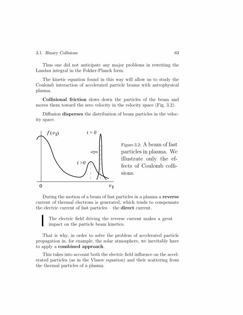
Collisional friction slows down the particles of the beam andmoves them toward the zero velocity in the velocity space (Fig. 3.2).
Diffusion disperses the distribution of beam particles in the veloc-ity space.
v
f
0 ||
( )v || t = 0
t >0
Figure 3.2: A beam of fastparticles in plasma. Weillustrate only the ef-fects of Coulomb colli-sions.
During the motion of a beam of fast particles in a plasma a reversecurrent of thermal electrons is generated, which tends to compensatethe electric current of fast particles – the direct current.
The electric field driving the reverse current makes a greatimpact on the particle beam kinetics.
That is why, in order to solve the problem of accelerated particlepropagation in, for example, the solar atmosphere, we inevitably haveto apply a combined approach.
This takes into account both the electric field influence on the accel-erated particles (as in the Vlasov equation) and their scattering fromthe thermal particles of a plasma.
64 Chapter 3. Weakly-Coupled Systems
3.2 Correlations and Debye-Huckel shielding
We are going to understand the most fundamental property of the bi-nary correlation function.
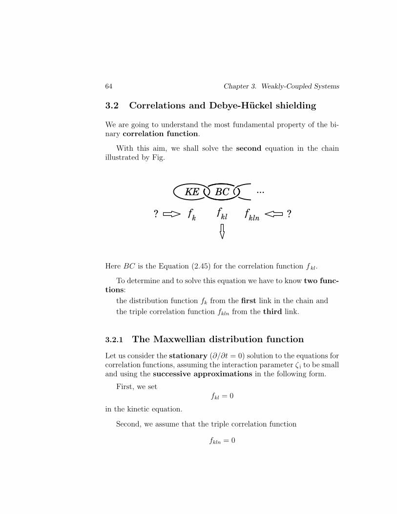
With this aim, we shall solve the second equation in the chainillustrated by Fig.
KE
fk
fkl f
kln
...BC
??
Here BC is the Equation (2.45) for the correlation function f kl.
To determine and to solve this equation we have to know two func-tions:
the distribution function fk from the first link in the chain and
the triple correlation function fkln from the third link.
3.2.1 The Maxwellian distribution function
Let us consider the stationary (∂/∂t = 0) solution to the equations forcorrelation functions, assuming the interaction parameter ζ i to be smalland using the successive approximations in the following form.
First, we setfkl = 0
in the kinetic equation.
Second, we assume that the triple correlation function
fkln = 0
3.2. Debye-Huckel Shielding 65
in Equation (2.45) for the correlation function fkl etc.
The plasma is supposed to be stationary, uniform and in thethermodynamic equilibrium state, i.e. the velocity distribution isassumed to be a Maxwellian function
fk (X) = fk (v2) = ck exp
(− mk v2
2kBTk
). (3.13)
The constant ck is determined by the normalizing condition and equals
ck = nk
(mk
2π kBTk
)3/2
.
It is obvious that the Maxwellian function satisfies the kinetic equa-tion under assumptions made above if the averaged force is equalto zero:
F k,α(X, t) = F k,α(X) = 0 . (3.14)
Since we shall need the same assumption in the next Section, weshall justify it there.
3.2.2 The averaged force and electric neutrality
Let us substitute the Maxwellian function in the kinetic equation, ne-glecting all the interactions except the Coulomb ones.
We obtain the following expression for the averaged force:
F k,α (X1) =∑
l
∫
X2
F kl,α (X1, X2) fl (X2) dX2 =
since plasma is uniform, fl does not depend of r2
=∑
l
∫
r2
F kl,α (r1, r2) d 3r2 ·∫
v2
fl (v2) d 3v2 =
66 Chapter 3. Weakly-Coupled Systems
= −∫
r2
∑
l
∂
∂r1,α
(ek el
| r1 − r2 |
)d 3r2 · nl =
= −∫
r2
∂
∂r1,α
(ek
| r1 − r2 |
)d 3r2 ·
∑
l
nl el . (3.15)
Therefore
F k,α = 0 , (3.16)
if the plasma is assumed to be electrically neutral:
∑
l
nl el = 0 .
(3.17)
Balanced charges of ions and electrons determine the nameplasma according Langmuir (1928).
So the averaged (statistically smoothed) force (2.32) is equal to zeroin the electrically neutral plasma but is not equal to zero in a systemof charged particles of the same charge sign: positive or negative, itdoes not matter.
Such a system tends to expand.
There is no neutrality in gravitational systems like stellar clus-ters.
The large-scale gravitational field makes an overall thermody-namic equilibrium impossible.
Moreover, on the contrary to plasma, they tend to contract andcollapse.
3.2. Debye-Huckel Shielding 67
3.2.3 Pair correlations and the Debye-Huckel radius
As a first approximation, on putting the triple correlation function
fkln = 0 ,
we obtain from Equation (2.45), in view of condition (3.16), the follow-ing equation for the binary correlation function fkl :
v 1,α∂fkl
∂ r1,α
+ v 2,α∂fkl
∂ r2,α
=
= −∑n
∫
X3
1
mk
F kn,α (X1, X3) fnl (X3, X2)∂fk
∂ v 1,α
+
+1
ml
F ln,α (X2, X3) fnk (X3, X1)∂fl
∂ v 2,α
dX3 . (3.18)
Let us consider the particles of two kinds: electrons and ions, as-suming the ions to be motionless and homogeneously distributed.
Then the ions do not take part in any kinetic processes.
Hence
ϕ i ≡ 0
for ions; and the correlation functions associated with ϕ i equal zerotoo:
f ii = 0 , fei = 0 etc. (3.19)
Among the pair correlation functions, only one has a non-zeromagnitude
fee (X1, X2) = f (X1, X2) . (3.20)
Taking into account (3.19), (3.20), and (3.13), rewrite Equation (3.18)as follows
68 Chapter 3. Weakly-Coupled Systems
v1∂f
∂ r1
+ v2∂f
∂ r2
=
=1
kBT
∫
X3
[v1 · F (X1, X3) f (X3, X2) fe (v1) +
+ v2 · F (X2, X3) f (X1, X3) fe (v2) ] dX3 . (3.21)
Since v1 and v2 are arbitrary and refer to the same kind of particles(electrons), (3.21) takes the form
∂f
∂ r1
=1
kBT
∫
X3
F (X1, X3) f (X3, X2) fe (v1) dX3 . (3.22)
Taking into account the Coulomb force in the same approxima-tion as (3.16) and assuming the correlation to exist only between thepositions of the particles in space (rather than between velocities), weintegrate both sides of (3.22) over d 3v1 d 3v2.
The result is
∂ g (r1, r2)
∂ r1
= − ne2
kBT
∫
r3
∇r1
1
| r1 − r3 | g (r2, r3) d 3r3 . (3.23)
Here the function
g (r1, r2) =∫
v1
∫
v2
f (X1, X2) d 3v1 d 3v2 . (3.24)
We integrate Equation (3.23) over r1 and designate the function
g (r1, r2) = g (r 212) ,
wherer12 = | r1 − r2 | .
3.2. Debye-Huckel Shielding 69
So we obtain the equation
g (r 212) = − ne2
kBT
∫
r3
g (r 223)
r13
d 3r3 .
Its solution is
g (r) =c 0
rexp
(− r
rDH
), (3.25)
where
rDH
=
(k
BT
4π ne2
)1/2
(3.26)
is the Debye-Huckel radius or, more exactly, the electron Debye-Huckel radius.
The constant of integration
c 0 = − 1
4π r 2DH
n(3.27)
(Exercise 3.8).
Substituting (3.27) in solution (3.25) gives the sought-after pair cor-relation function
g (r) = − 1
kBT
e2
rexp
(− r
rDH
). (3.28)
This formula shows that
the Debye-Huckel radius is a characteristic length of the paircorrelations in a fully-ionized equilibrium plasma.
As one might have anticipated,
the binary correlation function reproduces the shape of theactual potential of interaction, i.e. the shielded Coulombpotential:

70 Chapter 3. Weakly-Coupled Systems
g (r) ∼ ϕ (r) ∼ 1
rexp
(− r
rDH
).
(3.29)
Astrophysical plasmas exhibit collective phenomena arising outof mutual interactions of many particles.
Since the radius rDH
is a characteristic length of pair correlations,the number n r3
DHgives us a measure of the number of particles which
can interact simultaneously.
The inverse of this number is the so-called plasma parameter
ζp =(n r 3
DH
)−1. (3.30)
This is a small quantity as well as it can be expressed in terms of theinteraction parameter ζ i (Exercise 3.1).
In many astrophysical applications, the plasma parameter is reallysmall.
Thus, the number of particles inside the Debye-Huckel sphere is verylarge (Exercise 3.2).
So
the collective phenomena can be really important in astro-physical plasma in many places where it is weakly coupled.
3.3 Gravitational systems
A fundamental difference between the astrophysical plasmas andthe gravitational systems lies in the nature of the gravitational force:
there is no shielding to vitiate this long-range 1/r2 force.
The collisional integral formally equals infinity.
3.4. Numerical Simulations 71
The conventional wisdom of such systems asserts that they canbe described by the collisionless kinetic equation, the gravitationalanalog of the Vlasov equation.
Comment:
∞ ==> 0 !!!
On the basis of what we have seen above,
the collisionless approach in gravitational systems, i.e. theentire neglect of particle pair correlations, constitutes an un-controlled approximation.
Unlike the plasma, we cannot derive the next order correction to thecollisionless equation in the perturbation expansion.
We may hope to circumvent this difficulty by first identifying themean field force 〈F 〉, acting at any given point in space and thentreating fluctuations F ′ away from the mean field force.
However this is difficult to implement concretely because of the ap-parent absence of a clean separation of scales.
3.4 Comments on numerical simulations
The astrophysical plasma processes are typically investigated in welldeveloped and distinct approaches.
One approach, described by the Vlasov equation, is the collision-less limit used when collective effects dominate.
In cases where the plasma dynamics is determined by collision-al processes and where the self-consistent fields can be neglected, theFokker-Planck approach is used.
At the same time, it is known that
72 Chapter 3. Weakly-Coupled Systems
both collective effects and Coulomb collisions can play an es-sential role in a great variety of astrophysical phenomena.
Besides, collisions play the principal role in the physics ofcollisionless plasma.
Taking collisions into account may lead not only to quantitative butalso qualitative changes in the plasma behavior.
Even in the collisionless limit, the kinetic equation is difficult fornumerical simulations, and the ‘macroparticle’ method is widely usedalgorithms.
Instead of direct numerical solution of the kinetic equation, a set ofordinary differential equations for every macroparticle is solved.
These equations are the characteristics of the Vlasov equation.
In the case of a collisional plasma, the position of a macroparticlesatisfies the usual equation of the collisionless case
r ≡ d r
dt= v(t) . (3.31)
However the momentum equation is modified owing to the Coulombcollisions.
They are described by the Fokker-Planck operator (3.10) which in-troduces a friction and diffusion in velocity space.
Thus it is necessary to find the effective collisional force Fc whichacts on the macroparticles:
v ≡ dv
dt=
1
m(F
L+ Fc) . (3.32)
The collisional force can be introduced phenomenologically but a moremathematically correct approach can be constructed using the stochas-tic equivalence of the Fokker-Planck and Langevin equations.
Stochastic differential equations are regarded as an alternative
3.5. Practice: Exercises and Answers 73
to the description of astrophysical plasma in terms of distribution func-tion.
The Langevin approach allows one to overcome difficultiesrelated to the Fokker-Planck equation and to simulate actualplasma processes, taking account of both collective effects andCoulomb collisions.
Generally, if we construct a method for the simulation of complexprocesses in astrophysical plasma, we have to satisfy the following ob-vious but conflicting conditions.
First, the method should be adequate for the task in hand.
For a number of problems the simplified models of the collisionalintegral can provide a correct description and ensure a desired accuracy.
Second, the method should be computationally efficient.
The algorithm should not be extremely time-consuming.
In practice, some compromise between accuracy and complex-ity of the method should be achieved.
A ‘recipe’:
the choice of a particular model of the collisional integral isdetermined by the importance and particular features of thecollisional processes in a given astrophysical problem.
3.5 Practice: Exercises and Answers
Exercise 3.1. Show that the interaction parameter ζ i is related to theplasma parameter ζp as follows:
ζ i =1
4πζ 2/3
p . (3.33)
74 Chapter 3. Weakly-Coupled Systems
Exercise 3.2. How many particles are inside the Debye-Huckel spherein plasma of the solar corona?
Answer.
For an electron-proton plasma with T ≈ 2 × 10⁶ K and n ≈ 2 ×108 cm−3, the Debye-Huckel radius
rDH
=
(kT
8π e2 n
)1/2
≈ 4.9(
T
n
)1/2
≈ 0.5 cm . (3.34)
The number of particles inside the Debye-Huckel sphere
NDH
= n4
3πr3
DH∼ 108. (3.35)
Hence the typical value of plasma parameter in the corona is reallysmall:
ζ p ∼ 10−8 .
The interaction parameter is also small:
ζ i ∼ 10−6 .
Exercise 3.3. Estimate the interaction parameter (3.2) in the interiorof white dwarf stars (see also Exercise 1.3).
Exercise 3.4. Let w = w (v, δv) be the probability that a test particlechanges its velocity v to v + δv in the time interval δt.
The velocity distribution at the time t can be written as
f(v, t) =∫
f(v − δv, t− δt) w (v − δv, δv) d 3δv . (3.36)
Show that
the Fokker-Planck equation follows from the Taylor series ex-pansion of the function f(v, t) given by formula (3.36).
3.5. Practice: Exercises and Answers 75
Exercise 3.5. Express the collisional integral in terms of the differen-tial cross-sections of interaction between particles.
Exercise 3.6. Show that
the Fokker-Planck collisional model can be derived from theBoltzmann collisional integral
under the assumption that the change in the velocity of a particle dueto a collision is rather small.
Exercise 3.7. The Landau integral is generally thought to approx-imate the Boltzmann integral for the 1/r potential to a ‘dominantorder’, i.e. to within terms of order 1/lnΛ, where lnΛ is the Coulomblogarithm.
However this is not the whole truth.
Show that
the Landau integral approximates the Boltzmann integral tothe dominant order only in parts of the velocity space.
Exercise 3.8. Find the constant of integration c 0 in formula (3.25).
Exercise 3.9. Write and discuss the gravitational analog of the Vlasovequation.
Answer.
The basic assumption is that the gravitational N -body system canbe described in terms of a statistically smooth distribution function f (X, t).
The Vlasov equation manifests that this function will stream freelyin the self-consistent gravitational potential φ (r, t) associated with f (X, t),so that
∂f (X, t)
∂t+ vα
∂f (X, t)
∂rα
− ∂φ
∂rα
∂f (X, t)
∂vα
= 0 . (3.37)
Here
76 Chapter 3. Weakly-Coupled Systems
∆φ = − 4π Gρ (r, t) (3.38)
and
ρ (r, t) =∫
f (r,v, t) d 3v . (3.39)
Note that, in the context of the mean field theory, a distribution ofparticles over their masses has no effect.
Applying for example to the system of stars in a galaxy, Equa-tion (3.37) implies that
the net gravitational force acting on a star is determined bythe large-scale structure of the galaxy rather than by whetherthe star happens to lie close to some other star.
The force acting on any star does not vary rapidly, and each star issupposed to accelerate smoothly through the force field generated bythe galaxy as a whole.
In fact, gravitational encounters are not screened, they canbe thought of as leading to an additional collisional term on the rightside of the equation – a collisional integral.
However very little is known mathematically about such possibility.
Exercise 3.10. Discuss a gravitational analog of the Landau integralin the following form
(∂f
∂t
)
c
= σ∂
∂ v
∫
v ′
∂2 |v − v ′ |∂ v ∂ v ′ ·
(∂
∂ v− ∂
∂ v ′
)×
× [ f(r, v, t) f(r, v ′, t) ] d 3v ′ . (3.40)
Here σ is a constant determined by the effective collision rate.
Chapter 4
Macroscopic Description ofAstrophysical Plasma
In this Chapter we treat individual kinds of particles as con-tinuous media, mutually penetrating charged gases whichinteract between themselves and with an electromagneticfield.
This approach gives us the multi-fluid model which isuseful to consider many properties of astrophysical plasmas,e.g., the solar wind.
4.1 Summary of microscopic description
The kinetic equation gives us a microscopic (though averaged in astatistical sense) description of plasma.
Let us consider the transition to a less comprehensive macroscopicdescription.
We start from the kinetic equation for particles of kind k
∂fk (X, t)
∂t+ vα
∂fk (X, t)
∂rα
+
+F k,α (X, t)
mk
∂fk (X, t)
∂vα
=
(∂fk
∂t
)
c
. (4.1)
77
78 Chapter 4. Macroscopic Description of Plasma
Here the statistically averaged force is
F k,α (X, t) =∑
l
∫
X1
F kl,α (X,X1) fl (X1, t) dX1 (4.2)
and the collisional integral
(∂fk
∂t
)
c
= − ∂
∂vα
J k,α (X, t) , (4.3)
where the flux of particles of kind k
J k,α (X, t) =∑
l
∫
X1
1
mk
F kl,α (X,X1) f kl (X, X1, t) dX1 (4.4)
in the 6D phase space X = r,v.
4.2 Definition of macroscopic quantities
Before the deduction of equations for the macroscopic quantities ormacroscopic transfer equations, let us define the following momentsof the distribution function.
(a) The zeroth moment (without multiplying the distribution func-tion fk by the velocity v)
∫
v
fk (r,v, t) d 3v = nk(r, t) (4.5)
is the number of particles of kind k in a unit volume.
It is related to the mass density of particles of kind k
ρk(r, t) = mk nk(r, t) .
The plasma mass density is accordingly
4.2. Definition of Macroscopic Quantities 79
ρ (r, t) =∑
k
mk nk(r, t) . (4.6)
(b) The first moment of the distribution function, i.e. the integralof the product of the velocity v to the first power and the distributionfunction fk,
∫
v
vα fk(r,v, t) d 3v = nk uk,α (4.7)
is the particle flux, i.e. product of the number density by their meanvelocity
uk,α(r, t) =1
nk
∫
v
vα fk(r,v, t) d 3v . (4.8)
Consequently, the mean momentum of particles of kind k in a unitvolume is expressed as follows
mk nk uk,α = mk
∫
v
vα fk(r,v, t) d 3v . (4.9)
(c) The second moment of the distribution function is defined tobe
Π(k)αβ (r, t) = mk
∫
v
vαvβ fk (r,v, t) d 3v =
= mknk uk,αuk,β + p(k)αβ . (4.10)
Here we have introduced
v ′α = vα − uk,α
which is the deviation of the particle velocity from its mean value (4.8),so that
〈 v ′α 〉v = 0 ;
80 Chapter 4. Macroscopic Description of Plasma
and
p(k)αβ = mk
∫
v
v ′αv ′β fk (r,v, t) d 3v , (4.11)
is the pressure tensor.
Π(k)αβ is the tensor of momentum flux for particles of kind k.
Its component Π(k)αβ is the αth component of the momentum trans-
ported by the particles of kind k, in a unit time, across the unit areaperpendicular to the axis rβ.
Once we know the distribution function fk (r,v, t), we can derive allmacroscopic quantities related to these particles.
So, higher moments of the distribution function will be introducedas needed.
4.3 Macroscopic transfer equations
Note that the deduction of macroscopic equations is just derivation ofthe equations for the distribution function moments.
4.3.1 Equation for the zeroth moment
Let us calculate the zeroth moment of the kinetic equation:
∫
v
∂fk
∂td 3v +
∫
v
vα∂fk
∂rα
d 3v +
+∫
v
Fk,α
mk
∂fk
∂vα
d 3v =∫
v
(∂fk
∂t
)
c
d 3v . (4.12)
We interchange the order of integration over velocities and the dif-ferentiation with respect to time t in the first term and with respect tocoordinates rα in the second one.

4.3. Macroscopic Transfer Equations 81
Under the second integral
vα∂fk
∂rα
=∂
∂rα
(vαfk)− fk∂vα
∂rα
=∂
∂rα
(vαfk)− 0 ,
since r and v are independent variables in the phase space X.
Taking into account that the distribution function quickly ap-proaches zero as v → ∞, the integral of the third term is takenby parts and equals zero (Exercise 4.1).
The integral of the right-hand side of (4.12) describes the changein the number of particles of kind k as a result of collisions withparticles of other kinds.
If the processes of transformation, during which the particle kindcan be changed (such as ionization, recombination, charge exchangeetc., see Exercise 4.2), are not allowed for, then the last integral is zeroas well:
∫
v
(∂fk
∂t
)
c
d 3v = 0 . (4.13)
Thus, by integration of (4.12), the following equation is found
∂nk
∂t+
∂
∂rα
nk uk,α = 0 .
(4.14)
This is the continuity equation expressing the conservation of parti-cles of kind k or (i.e. the same, of course) conservation of their mass:
∂ρk
∂t+
∂
∂rα
ρk uk,α = 0 . (4.15)
Equation (4.14) for the zeroth moment nk depends on theunknown first moment uk,α.
This is illustrated by Fig. 4.1.
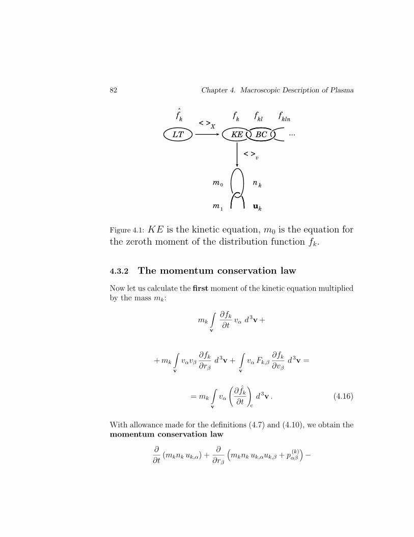
82 Chapter 4. Macroscopic Description of Plasma
LT KE
fk
fk
fkl
< >X
< >v
n
u
nk
k
fkln
...BC
m
m1
0
Figure 4.1: KE is the kinetic equation, m0 is the equation forthe zeroth moment of the distribution function fk.
4.3.2 The momentum conservation law
Now let us calculate the first moment of the kinetic equation multipliedby the mass mk:
mk
∫
v
∂fk
∂tvα d 3v +
+ mk
∫
v
vαvβ∂fk
∂rβ
d 3v +∫
v
vα Fk,β∂fk
∂vβ
d 3v =
= mk
∫
v
vα
(∂fk
∂t
)
c
d 3v . (4.16)
With allowance made for the definitions (4.7) and (4.10), we obtain themomentum conservation law
∂
∂t(mknk uk,α) +
∂
∂rβ
(mknk uk,αuk,β + p
(k)αβ
)−
4.3. Macroscopic Transfer Equations 83
−〈F k,α(r, t) 〉v = 〈F (c)k,α (r, t) 〉v . (4.17)
Here p(k)αβ is the pressure tensor (4.11), i.e. a part of the unknown second
moment (4.10).
The mean force acting on the particles of kind k in a unit volumeis
〈F k,α (r, t) 〉v =∫
v
F k,α (r,v, t) fk (r,v, t) d 3v . (4.18)
In the case of the Lorentz force, the mean force
〈F k,α (r, t) 〉 v = nkek
[Eα +
1
c(uk ×B )α
]
or
〈F k,α (r, t) 〉 v = ρ qk Eα +
1
c( j q
k ×B )α .(4.19)
Here ρ qk and j q
k are the mean densities of electric charge and current,produced by the particles of kind k.
Note that
the mean electromagnetic force couples all the charged com-ponents of astrophysical plasma together
because the electric and magnetic fields, E and B, act on all chargedcomponents and, at the same time, all charged components contributeto the electric and magnetic fields according to Maxwell’s equations.
The right-hand side of Equation (4.17) contains the mean force re-sulting from collisions, the mean collisional force
〈F (c)k,α (r, t) 〉 v = mk
∫
v
vα
(∂fk
∂t
)
c
d 3v . (4.20)
84 Chapter 4. Macroscopic Description of Plasma
Substituting (4.3) in definition (4.20) and integrating gives us themost general formula for the mean collisional force
〈F (c)k,α (r, t) 〉 v = mk
∫
v
J k,α (r,v, t) d 3v = (4.21)
=∑
l 6=k
∫
v
∫
v1
∫
r1
F kl,α (r,v, r1,v1) fkl (r,v, r1,v1, t) d 3r1 d 3v1 d 3v .
Note that
for the particles of the same kind, the elastic collisions cannotchange the total particle momentum per unit volume.
That is why l 6= k in the sum (4.21).
Formula (4.21) contains the unknown binary correlation function fkl.
The last should be found from the correlation function Equation (2.45)indicated as the second link BC in Fig. 4.2.
Thus
the equation for the first moment of the distribution functionis as much unclosed as the initial kinetic equation.
Therefore the equation for the first moment is unclosed in two direc-tions.
If each of kinds of particles is in thermodynamic equilibrium, thenthe mean collisional force can be expressed in terms of the mean mo-mentum loss during the collisions of a particle of kind k with theparticles of other kinds:
〈F (c)k,α (r, t) 〉 v = −∑
l 6=k
mknk (uk,α − ul,α)
τkl
.
(4.22)
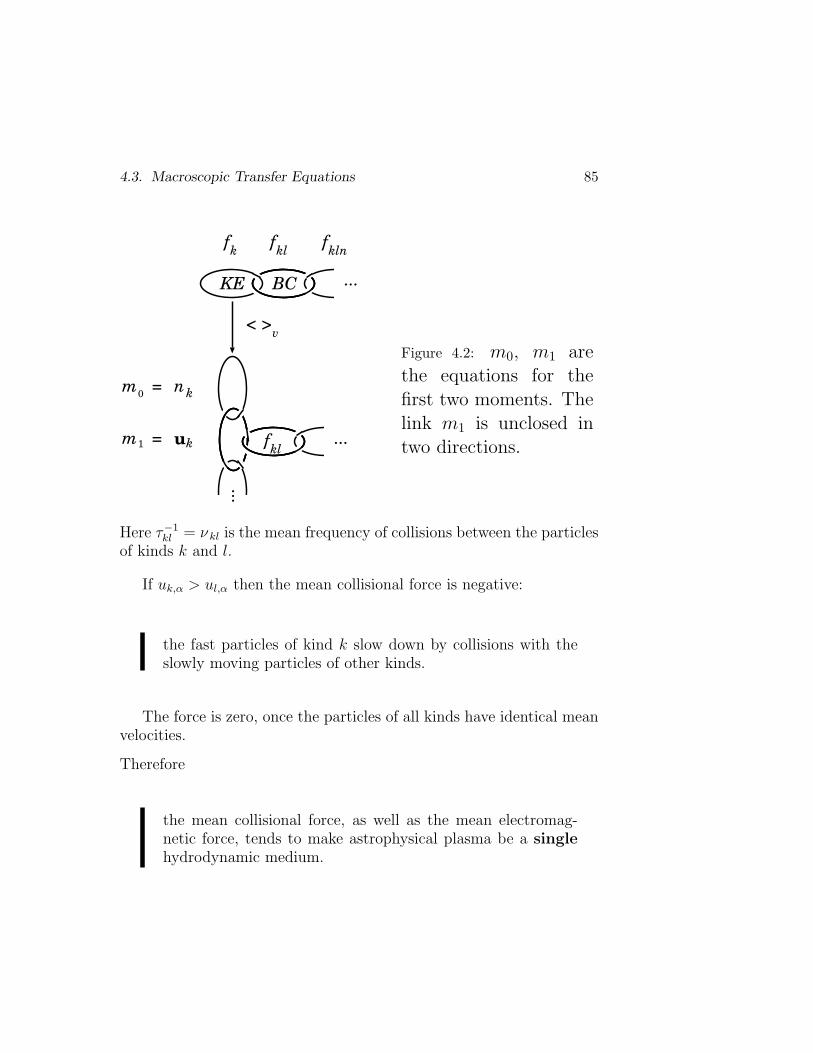
4.3. Macroscopic Transfer Equations 85
KE
fk
fkl
< >v
n
u
nk
k
fkln
...BC
m
m ...
...
fkl
0
1
=
=
Figure 4.2: m0, m1 arethe equations for thefirst two moments. Thelink m1 is unclosed intwo directions.
Here τ−1kl = ν kl is the mean frequency of collisions between the particles
of kinds k and l.
If uk,α > ul,α then the mean collisional force is negative:
the fast particles of kind k slow down by collisions with theslowly moving particles of other kinds.
The force is zero, once the particles of all kinds have identical meanvelocities.
Therefore
the mean collisional force, as well as the mean electromag-netic force, tends to make astrophysical plasma be a singlehydrodynamic medium.
86 Chapter 4. Macroscopic Description of Plasma
4.4 The energy conservation law
4.4.1 The second moment equation
The second moment of a distribution function fk is the tensor of mo-mentum flux density
Π(k)αβ (r, t) = mk
∫
v
vαvβ fk (r,v, t) d 3v =
= mknk uk,αuk,β + p(k)αβ .
In order to find an equation for this tensor, we should multiply thekinetic equation
∂fk
∂t+ vα
∂fk
∂rα
+F k,α
mk
∂fk
∂vα
=
(∂fk
∂t
)
c
by the factor mk vαvβ and integrate over velocity space v.
In this way, we could arrive to a matrix equation in partial deriva-tives.
If we take the trace of this equation we obtain the partial differentialscalar equation for energy density of the particles.
This is the correct self-consistent way which is the basis of the mo-ment method.
For our aims, a simpler direct procedure is sufficient and correct.
In order to derive the energy conservation law, we multiplyEquation (4.1) by the particle’s kinetic energy
mkv2α/2
and integrate over velocities, taking into account that
vα = uk,α + v ′α , 〈 v ′α 〉v = 0 ,
and
4.4. The energy conservation law 87
v 2α = u 2
k,α + (v ′α)2+ 2 uk,α v ′α .
A straightforward integration yields
∂
∂t
(ρku
2k
2+ ρk εk
)+
+∂
∂rα
[ρkuk,α
(u 2
k
2+ εk
)+ p
(k)αβ uk,β + q k,α
]=
= ρ qk (E · uk) +
(F
(c)k · uk
)+ Q
(c)k (r, t) + L (r)
k (r, t) . (4.23)
Here
mk εk(r, t) =1
nk
∫
v
mk (v ′α)2
2fk (r,v, t) d 3v =
=mk
2nk
∫
v
(v ′α)2
fk (r,v, t) d 3v (4.24)
is the mean kinetic energy of chaotic (non-directed) motion persingle particle of kind k.
Thus the first term on the left-hand side of (4.23) represents thetime derivative of the energy of the particles of kink k in a unit volume,which is the sum of kinetic energy of a regular motion with the meanvelocity uk and the so-called internal energy.
As every tensor, the pressure tensor can be written as
p(k)αβ = pk δαβ + π
(k)αβ . (4.25)
On rearrangement, we obtain the following general equation
∂
∂t
(ρku
2k
2+ ρk εk
)+
88 Chapter 4. Macroscopic Description of Plasma
+∂
∂rα
[ρkuk,α
(u 2
k
2+ wk
)+ π
(k)αβ uk,β + q k,α
]=
= ρ qk (E · uk) +
(F
(c)k · uk
)+ Q
(c)k (r, t) + L (r)
k (r, t) . (4.26)
Here
wk = εk +pk
ρk
(4.27)
is the heat function per unit mass.
Therefore the second term on the left-hand side contains the energyflux
ρkuk,α
(u 2
k
2+ wk
),
which can be called the ‘advective’ flux of kinetic energy.
Let us mention the known astrophysical application of this term.
The advective cooling of ions heated by viscosity might dominatethe cooling by the electron-ion collisions, e.g., in a high-temperatureplasma flow near a rotating black hole.
In an advection-dominated accretion flow (ADAF), the heatgenerated via viscosity is transferred inward the black hole rather thanradiated away locally like in a standard accretion disk model.
However, discussing the ADAF as a solution for the important as-trophysical problem should be treated with reasonable cautions.
Looking at Equations (4.23) for electrons and ions separately, wesee that
too many assumptions have to be made to arrive to the ADAFapproximation.
4.4. The energy conservation law 89
For example, this is not realistic to assume that plasma electronsare heated only due to collisions with ions and, for this reason, theelectrons are much cooler than the ions.
The suggestions underlying the ADAF model ignore several effectsincluding reconnection and dissipation of magnetic fields (regular andrandom) in astrophysical plasma.
This makes a physical basis of the ADAF model uncertain.
4.4.2 The case of thermodynamic equilibrium
In order to clarify the definitions given above, let us, for a while, comeback to the general principles.
If the particles of the kth kind are in the thermodynamic equilib-rium, then fk is the Maxwellian function with the temperature Tk:
f(0)
k (r,v) = nk(r)
[mk
2π kBTk(r)
]3/2
×
× exp
− mk |v − uk(r) | 2
2 kBTk(r)
. (4.28)
In this case, according to (4.24), the mean kinetic energy of chaoticmotion per single particle of kind k
mk εk =3
2k
BTk . (4.29)
The pressure tensor (4.11) is isotropic:
p(k)αβ = pk δαβ , (4.30)
where the scalar
pk = nk kBTk (4.31)
is the gas pressure of the particles of kind k.
90 Chapter 4. Macroscopic Description of Plasma
This is also the equation of state for the ideal gas.
Thus we have found that the pressure tensor is diagonal.
This implies the absence of viscosity for the ideal gas:
π(k)αβ = 0 . (4.32)
The heat function per unit mass or, more exactly, the specificenthalpy is
wk = εk +pk
ρk
=5
2
kBTk
mk
. (4.33)
It was a particular case of the thermodynamic equilibrium.
4.4.3 The general case of anisotropic plasma
In general, we do not expect that the particles of kind k have reachedthermodynamic equilibrium.
Nevertheless we often use the mean kinetic energy (4.24) to definethe effective kinetic temperature Tk according to definition (4.29).
A kinetic temperature is just a measure for the spread of theparticle distribution in velocity space.
The kinetic temperatures of different components in astrophysicalplasma may differ from each other.
Moreover, in an anisotropic plasma, the kinetic temperatures par-allel and perpendicular to the magnetic field are different.
Without supposing thermodynamic equilibrium, in an anisotro-pic plasma, the part associated with the deviation of the distributionfunction from the isotropic one is distinguished in the pressure tensor:
p(k)αβ − pk δαβ = π
(k)αβ . (4.34)
4.4. The energy conservation law 91
Here π(k)αβ is called the viscous stress tensor.
Recall that we did not derive an equation for this tensor.
The term π(k)αβ uk,β in equation (4.23) represents the flux of energy
released by the viscous force in the particles of kind k.
The last term on the left-hand side of the energy equation, the vector
q k,α =∫
v
mk (v ′)2
2v ′α fk (r,v, t) d 3v (4.35)
is the heat flux density due to the particles of kind k.
Formula (4.35) shows that a third-order-moment term appearsin the second order moment of the kinetic equation.
The right-hand side of the energy conservation law (4.23) containsthe following four terms:
(a) The first term
ρ qk (E · uk) = nkek Eα uk,α (4.36)
is the work done by the Lorentz force (without the magnetic field, ofcourse) in unit time on unit volume.
(b) The second term
(F
(c)k · uk
)= uk,α
∫
v
mk v ′α
(∂fk
∂t
)
c
d 3v (4.37)
is the work done by the collisional force of friction of the particles ofkind k with all other particles in unit time on unit volume.
The work of friction force results from the mean momentumchange of particles of kind k (moving with the mean velocityuk) owing to collisions with all other particles.
92 Chapter 4. Macroscopic Description of Plasma
This work equals zero if uk = 0.
(c) The third term
Q(c)k (r, t) =
∫
v
mk (v ′)2
2
(∂fk
∂t
)
c
d 3v (4.38)
is the rate of thermal energy release (heating or cooling) in a gas of theparticles of kind k due to collisions with other particles.
Recall that the collisional integral depends on the binary correla-tion function fkl.
(d) The last term L (r)k (r, t) takes into account that a plasma com-
ponent k can gain energy by absorbing radiations of different kinds andcan lose the energy by emitting radiations.
4.5 General properties of transfer equations
4.5.1 Divergent and hydrodynamic forms
Equations (4.14), (4.17), and (4.23) are referred to as the equations ofparticle, momentum and energy transfer.
They are written in the ‘divergent’ form.
This essentially states the conservation laws and turns out to beconvenient in numerical work, to construct the conservative schemesfor computations.
Sometimes, other forms are more convenient.
For instance, the equation of momentum transfer or simply the equa-tion of motion can be brought into the frequently used form:
ρk
(∂ uk,α
∂t+ uk,β
∂ uk,α
∂rβ
)= − ∂
∂rβ
p(k)αβ +
+ 〈F k,α (r, t) 〉 v + 〈F (c)k,α (r, t) 〉 v . (4.39)
4.5. Properties of the Transfer Equations 93
The so-called substantial derivative appears on the left-hand side ofthis equation:
d (k)
dt=
∂
∂t+ uk,β
∂
∂rβ
=∂
∂t+ uk · ∇r .
(4.40)
This substantial or advective derivative – the total time derivativefollowing a fluid element of kind k – is typical of hydrodynamic-type equations, to which the equation of motion (4.39) belongs.
In the frame, in which the fluid element is not moving, themean velocity uk = 0 but the time partial derivative ∂/∂tdoes not vanish of course.
The total time derivative with respect to the mean velocity uk of theparticles of kind k is different for each kind k.
In the one-fluid MHD theory, we shall introduce the substantialderivative with respect to the average velocity of the plasma as a whole.
For the case of the Lorentz force, the equation of motion of theparticles of kind k can be rewritten as follows:
ρkd (k) uk,α
dt= − ∂
∂rβ
p(k)αβ + ρ q
k Eα +1
c( j q
k ×B )α +
+ 〈F (c)k,α (r, t) 〉 v . (4.41)
Here the right-hand side represents the forces acting on the fluid ele-ment of kind k, in particular, the last term is the mean collisionalforce.
The left-hand side of (4.41) is the change of the momentum of thisfluid element.
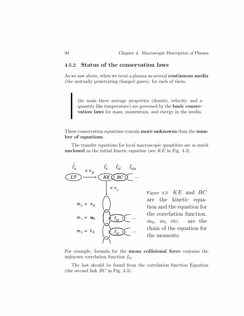
94 Chapter 4. Macroscopic Description of Plasma
4.5.2 Status of the conservation laws
As we saw above, when we treat a plasma as several continuous media(the mutually penetrating charged gases), for each of them,
the main three average properties (density, velocity, and aquantity like temperature) are governed by the basic conser-vation laws for mass, momentum, and energy in the media.
These conservation equations contain more unknowns than the num-ber of equations.
The transfer equations for local macroscopic quantities are as muchunclosed as the initial kinetic equation (see KE in Fig. 4.3).
LT KE
fk
fk
fkl
< >X
< >v
n
u
n
ε
k
k
k
fkln
...BC
m
m
m
...
...
fkl
fkl
0
1
2
=
=
=
Figure 4.3: KE and BC
are the kinetic equa-tion and the equation forthe correlation function.m0, m1 etc. are thechain of the equation forthe moments.
For example, formula for the mean collisional force contains theunknown correlation function fkl.
The last should be found from the correlation function Equation(the second link BC in Fig. 4.3).
4.6. Equation of State and Transfer Coefficients 95
The terms (4.37) and (4.38) in the energy conservation equation alsodepend on the unknown function fkl.
It is also important that the transfer equations are unclosed in ‘or-thogonal’ direction:
Equation for the zeroth moment (the link m0 in Fig. 4.3), density nk,depends on the unknown first moment, the mean velocity uk, and soon.
This process of generating equations for the higher momentscould be extended indefinitely depending solely on how many primaryvariables (nk, uk, εk, ...) we are prepared to introduce.
Anyway we know now that
the conservation laws for mass, momentum, and energy in thecomponents of astrophysical plasma represent the first threelinks in the chain of equations for the distribution functionmoments.
It certainly would not be easy (if possible) to arrive to this fundamentalconclusion
andwould be difficult to derive the conservation laws in the form of
the transfer Equations (4.14), (4.17), and (4.23) in the way which istypical for the majority of textbooks: from simple specific knowledgeto more general ones.
4.6 Equation of state and transfer coefficients
The first three transfer equations for a plasma component k would beclosed with respect to the three unknown variables ρk, uk, and εk,
if it were possible to express the other unknown quantities pk, π(k)αβ ,
q (k)α , etc. in terms of these three variables.
Thus, we have to know the equation of state and the so-calledtransfer coefficients.
96 Chapter 4. Macroscopic Description of Plasma
How can we find them?
Formally, we should write equations for higher moments of thedistribution function.
However these equations will not be closed either.
So, how shall we proceed?
According to the general principles of statistical physics,
by virtue of collisions in a closed system of particles, any dis-tribution function tends to assume the Maxwellian form.
The Maxwellian distribution is the kinetic equation solution for astationary homogeneous gas in the absence of any mean force in thethermal equilibrium, i.e. for a gas in thermodynamic equilibrium.
Then spatial gradients and derivatives with respect to time are zero.
In fact they are always nonzero.
For this reason, the assumption of full thermodynamic equilibriumis replaced with the local thermodynamic equilibrium (LTE).
Moreover
if the gradients and derivatives are small, then the real distri-bution function differs little from the local Maxwellian one,the difference being proportional to the small gradients orderivatives.
If we are interested in a process occurring in a time t, which is muchgreater than the collision time τ , and at a distance L, which is muchlarger than the mean free path λ,
t À τ , L À λ , (4.42)
then the distribution function fk(r,v, t) is a sum of the local Max-wellian distribution
4.6. Equation of State and Transfer Coefficients 97
f(0)
k (r,v, t) = nk(r, t)
[mk
2π kBTk(r, t)
]3/2
×
× exp
− mk |v − uk(r, t) | 2
2 kBTk(r, t)
(4.43)
and some small additional term f(1)
k (r,v, t).
Therefore
fk(r,v, t) = f(0)
k (r,v, t) + f(1)
k (r,v, t) . (4.44)
Since the function f(0)
k depends on t and r, we find the derivatives
∂f(0)
k /∂t and ∂f(0)
k /∂rα.
By using these derivatives, we substitute function (4.44) in the ki-netic equation and linearly approximate the collisional integral by usingone or another of the models introduced in Chapter 3; see also Exer-cise 4.5.
Then we seek the additional term f(1)
k in the linear approximation.
For example, in the case of the heat flux qα, the flux qα is chosen tobe proportional to the temperature gradient.
Thus, in a fully ionized plasma without magnetic field, the heatflux in the electron component of plasma
q e = −κ e∇Te , (4.45)
where
κ e ≈ 1.84× 10⁻⁵
lnΛT 5/2
e (4.46)
is the coefficient of electron thermal conductivity.
In the presence of strong magnetic field in astrophysical plasma,all the transfer coefficients become highly anisotropic.
98 Chapter 4. Macroscopic Description of Plasma
Since the Maxwellian function and its derivatives are determined bythe parameters nk, uk, and Tk, the transfer coefficients are expressedin terms of the same quantities and magnetic field B, of course.
This procedure makes it possible to close the set of transferequations for astrophysical plasma
under the conditions (4.42).
∗ ∗ ∗
The first three moment equations were extensively used in astro-physics, for example, in investigations of the solar wind.
They led to a significant understanding of phenomena such as es-cape, acceleration and cooling.
However, as more detailed observations become available, it ap-peared that the collisionally dominated models are not adequatefor most physical states of the solar wind.
A higher order, closed set of equations for the six moments havebeen derived for multi-fluid, moderately non-Maxwellian plasmaof the solar wind.
On this basis, the generalized expression for heat flux relates theflux to the temperature gradients, relative streaming velocity, thermalanisotropy, temperature differences of the components.
4.7 Gravitational systems
There is a big difference between astrophysical plasmas and astrophys-ical gravitational systems (Sect. 3.3).
The gravitational attraction cannot be screened.
A large-scale gravitational field always exists over a system be-cause the neutrality condition (3.17) cannot be satisfied.
4.7. Gravitational Systems 99
The large-scale gravitational field makes an overall thermody-namic equilibrium impossible.
Therefore
those results of plasma astrophysics which explicitly dependupon the plasma being in thermodynamic equilibrium do nothold for gravitational systems.
For systems, like the stars in a galaxy, we may hope that the ob-served distribution function reflects something about the initial con-ditions rather than just the relaxation mechanism.
So galaxies may be providing us with clues on how they wereformed.
∗ ∗ ∗
If we consider processes on a spatial scale which is large enough tocontain a large number of stars then one of the main requirements ofthe continuum mechanics is justified.
Anyway, several aspects of the structure of a galaxy can be under-stood in hydrodynamic approximation.
More often than never,
hydrodynamics provides a first level description of an astro-physical phenomenon governed predominantly by the gravi-tational force.
For example, the early stages of star formation during which aninterstellar cloud of low density collapses under the action of its owngravity can be modeled in the hydrodynamic approximation.
However, when we want to explain the difference between the an-gular momentum of the cloud and that of the born star, we have toinclude the effect of a magnetic field.
100 Chapter 4. Macroscopic Description of Plasma
Chapter 5
The Generalized Ohm’s Lawin Plasma
The multi-fluid models of astrophysical plasma allow us toderive the generalized Ohm’s law and to consider differentphysical approximations, including the collisional and col-lisionless plasma models.
5.1 The classic Ohm’s law
The usual Ohm’s law,
j = σE ,
relates the current j to the electric field E in a solid conductor inrest.
As we know, the electric field in every equation of motion determinesacceleration of particles rather than their velocity.
That is why, generally, such a simple relation as the classic Ohm’slaw does not exist.
Moreover, while considering astrophysical plasmas, it is necessaryto take into account the presence of a magnetic field and the motionof a plasma as a whole or as a medium consisting of several movingcomponents, their compressibility.
101
102 Chapter 5. Generalized Ohm’s Law
Recall the way of deriving the usual Ohm’s law.
The current is determined by the relative motion of electrons andions.
Let us assume that the ions do not move.
An equilibrium is set up between the electric field action and electrons-on-ions friction:
0 = − e ne Eα + mene νei ( 0− ue,α) ,
resulting in Ohm’s law
jα = − e ne ue,α = +e2ne
me νei
Eα = σEα . (5.1)
Here
σ =e2ne
me νei
(5.2)
is the electric conductivity.
In order to deduce the generalized Ohm’s law for a plasma withmagnetic field, we have to consider at least two equations of motion– for the electron and ion components.
5.2 Derivation of basic equations
Let us write the momentum equations for electrons and ions:
me∂
∂t(ne ue,α) = − ∂ Π
(e)αβ
∂rβ
− ene
[E +
1
c(ue ×B )
]
α+
+ mene νei (ui,α − ue,α) , (5.3)
mi∂
∂t(ni ui,α) = − ∂ Π
(i)αβ
∂rβ
+ Zi eni
[E +
1
c(ui ×B )
]
α+
5.2. Derivation of Basic Equations 103
+ mene νei (ue,α − ui,α) . (5.4)
Here the tensor of momentum flux
Π(e)αβ (r, t) = mene ue,α ue,β + p
(e)αβ (5.5)
andΠ
(i)αβ (r, t) = mini ui,α ui,β + p
(i)αβ . (5.6)
The last term in (5.3) represents the mean momentum transferred,because of collisions, between electrons and ions.
It is equal, with opposite sign, to the last term in Equation (5.4).
We assume that there are just two kinds of particles, their totalmomentum remaining constant under the action of elastic collisions.
Now let us suppose that the ions are protons (Zi = 1), and electricalneutrality occurs:
ni = ne = n .
Let us multiply (5.3) by −e/me and add it to (5.4) multipliedby e/mi.
The result is
∂
∂t[ en (ui,α − ue,α) ] =
[e
mi
F i,α − e
me
F e,α
]+
+ e2n(
1
me
+1
mi
)Eα +
e2n
c
[ (u e
me
×B)
α
+(
u i
mi
×B)
α
]−
− νei en[(ui,α − ue,α) +
me
mi
(ui,α − ue,α)]. (5.7)
Here
F e,α = − ∂ Π(e)αβ
∂rβ
and F i,α =∂ Π
(i)αβ
∂rβ
. (5.8)
104 Chapter 5. Generalized Ohm’s Law
Let us introduce the velocity of the centre-of-mass system
u =mi u i + me u e
mi + me
.
Since mi À me,
u = u i +me
mi
u e ≈ u i . (5.9)
On treating Equation (5.7), we neglect the small terms of the orderof the ratio me/mi.
We obtain the equation for the current
j = en (u i − u e)
in the system of coordinates (5.9).
This equation is
∂ j ′
∂t=
e2n
me
[E +
1
c(u×B )
]− e
mec( j ′ ×B )−
− νei j′ +
e
mi
Fi − e
me
Fe . (5.10)
The prime designates the current in the system of moving plasma, i.e.in the rest-frame of the plasma.
Let E u denote the electric field in this frame of reference, i.e.
E u = E +1
cu×B . (5.11)
Now we divide Equation (5.10) by νei and represent it in the form
j ′ =e2n
meνei
E u −ω (e)
B
νei
j ′ × n−
− 1
νei
∂ j ′
∂t+
1
νei
(e
mi
Fi − e
me
Fe
). (5.12)
5.2. Derivation of Basic Equations 105
Heren = B/B
and
ω (e)B
=eB
mec
is the electron gyro-frequency.
Thus we have derived a differential equation for the current j ′.
The third and the fourth terms on the right do not depend of mag-netic field.
Let us replace them by some effective electric field
σE eff = − 1
νei
∂ j ′
∂t+
e
νei
(1
mi
Fi − 1
me
Fe
), (5.13)
where
σ =e2n
me νei(5.14)
is the plasma conductivity in the absence of magnetic field.
Combine the fields (5.11) and (5.13),
E ′ = E u + E eff , (5.15)
in order to rewrite (5.12) in the form
j ′ = σE ′ − ω (e)B
νei
j ′ × n . (5.16)
We shall consider (5.16) as an algebraic equation in j ′, neglecting the∂ j ′/∂t dependence of the field (5.13).
Note, however, that
the term ∂ j ′/∂t is by no means small in the problem of theparticle acceleration by a strong electric field in astrophysi-cal plasma.
106 Chapter 5. Generalized Ohm’s Law
Collisionless reconnection is the phenomenon in which parti-cle inertia of the current replaces classical resistivity in allowing fastreconnection to occur.
5.3 The general solution
Let us find the solution to Equation (5.16) as a sum
j ′ = σ‖E′‖ + σ⊥E ′
⊥ + σHn× E ′
⊥ .(5.17)
Substituting (5.17) in (5.16) gives
σ ‖ = σ =e2n
meνei
, (5.18)
σ⊥ = σ1
1 +(ω (e)
Bτei
)2 , (5.19)
σH
= σω (e)
Bτei
1 +(ω (e)
Bτei
)2 . (5.20)
Formula (5.17) is called the generalized Ohm’s law.
A magnetic field in a plasma not only changes the magnitude of theconductivity, but the form of Ohm’s law as well:
the electric field and the resulting current are not parallel, since
σ⊥ 6= σ ‖ .
Thus the conductivity of a plasma in a magnetic field is anisotropic.
Moreover the current component j ′H
is perpendicular to both themagnetic and electric fields.
This component is the so-called Hall current (Fig. 5.1).
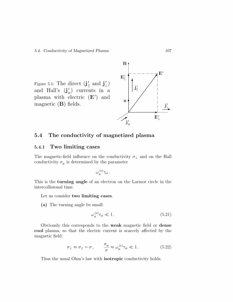
5.4. Conductivity of Magnetized Plasma 107
Figure 5.1: The direct (j ′‖ and j ′⊥)and Hall’s (j ′
H) currents in a
plasma with electric (E ′) andmagnetic (B) fields.
B 6
´´
´
E ′‖
j ′‖
j ′⊥
E ′
E ′⊥
j ′H
n
-
6
6
-
6
¶¶
¶¶
¶¶
¶¶
¶¶¶7
´3
5.4 The conductivity of magnetized plasma
5.4.1 Two limiting cases
The magnetic-field influence on the conductivity σ⊥ and on the Hallconductivity σ
His determined by the parameter
ω (e)B
τei .
This is the turning angle of an electron on the Larmor circle in theintercollisional time.
Let us consider two limiting cases.
(a) The turning angle be small:
ω (e)B
τei ¿ 1 . (5.21)
Obviously this corresponds to the weak magnetic field or densecool plasma, so that the electric current is scarcely affected by themagnetic field:
σ⊥ ≈ σ ‖ = σ ,σ
H
σ≈ ω (e)
Bτei ¿ 1 . (5.22)
Thus the usual Ohm’s law with isotropic conductivity holds.
108 Chapter 5. Generalized Ohm’s Law
(b) The opposite case, when the electrons spiral freely betweenrare collisions of electrons with ions:
ω (e)B
τei À 1 , (5.23)
corresponds to the strong magnetic field and hot rarefied plasma.
This plasma is termed the magnetized one.
It is frequently encountered under astrophysical conditions.
In this case
σ ‖ = σ ≈(ω (e)
Bτei
)σ
H≈
(ω (e)
Bτei
)2σ⊥ . (5.24)
Hence in a magnetized plasma, for example in the solar corona
σ‖ À σHÀ σ⊥ .
(5.25)
In other words,
the impact of the magnetic field on the direct current is es-pecially strong for the component resulting from the electricfield E ′
⊥.
The current in the E ′⊥ direction is considerably weaker than it would
be in the absence of a magnetic field.
Why?
5.4.2 The physical interpretation
The physical mechanism of the perpendicular current j ′⊥ is illustratedby Fig. 5.2.
The primary effect of the electric field E ′⊥ in the presence
of the magnetic field B is not the current in the direction E ′⊥,
but rather the electric drift in the direction perpendicular toboth B and E ′
⊥.
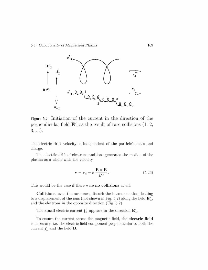
5.4. Conductivity of Magnetized Plasma 109
E
vd
Bv
d
p
e
+
-1
2
3
⊥
⊥j
u e⊥
Figure 5.2: Initiation of the current in the direction of theperpendicular field E ′
⊥ as the result of rare collisions (1, 2,3, ...).
The electric drift velocity is independent of the particle’s mass andcharge.
The electric drift of electrons and ions generates the motion of theplasma as a whole with the velocity
v = vd = cE×B
B 2. (5.26)
This would be the case if there were no collisions at all.
Collisions, even the rare ones, disturb the Larmor motion, leadingto a displacement of the ions (not shown in Fig. 5.2) along the field E ′
⊥,and the electrons in the opposite direction (Fig. 5.2).
The small electric current j ′⊥ appears in the direction E ′⊥.
To ensure the current across the magnetic field, the electric fieldis necessary, i.e. the electric field component perpendicular to both thecurrent j ′⊥ and the field B.
110 Chapter 5. Generalized Ohm’s Law
The Hall electric field balances the Lorentz force acting onthe carriers of the perpendicular electric current in a rarelycollisional plasma due to the presence of a magnetic field,
i.e. the force
F ( j ′⊥) =e n
cu i⊥ ×B− e n
cu e⊥ ×B =
=1
ce n (u i⊥ − u e⊥)×B (5.27)
Hence the magnitude of the Hall electric field is
E ′H
=1
en cj ′⊥ ×B . (5.28)
The Hall electric field in astrophysical plasma is frequently set upautomatically, as a consequence of small charge separation withinthe limits of quasi-neutrality.
In a fully-ionized rarely-collisional plasma, the tendency for aparticle to spiral round the magnetic field lines insures the great reduc-tion in the transversal conductivity.
However, since the dissipation of the energy of the electric currentinto Joule heat,
j ′E ′ ,
is due solely to collisions between particles (if the particle accelerationcan be neglected), the reduced conductivity does not lead to increaseddissipation.
On the other hand, the Hall electric field and Hall current cansignificantly modify conditions of magnetic reconnection.
Compared with ordinary resistive MHD, the Hall MHD reconnec-tion is distinguished by qualitatively different magnetic field distri-butions, electron and ion signatures in reconnecting current layers.
5.5. Currents and Charges in Plasma 111
Although the Hall effect itself is nondissipative,
j ′HE ′ = 0 , (5.29)
it can lead to dissipation through a turbulent “Hall cascade”, mag-netic energy cascading from large to small scales, where it dissipates byohmic decay.
The Hall effect can dominate ohmic decay of currents in the crust ofneutron stars and therefore can determine evolution of their magneticfield.
In an initial poloidal dipole field, the toroidal currents “twist” thefield.
The resulting poloidal currents then generate a quadrupole polo-idal field.
5.5 Currents and charges in plasma
5.5.1 Collisional and collisionless plasmas
Let us point out another property of the generalized Ohm’s law.
Under laboratory conditions, as a rule, one cannot neglect the gra-dient forces.
On the contrary, these forces usually play no part in astrophysicalplasma.
We shall often ignore them.
However this simplification may be not justified in reconnectingcurrent layers, shock waves and other discontinuities.
Let us also restrict our consideration to very slow (say hydrody-namic) motions of plasma.
These motions are supposed to be so slow that the following threeconditions are fulfilled.
(A) It is supposed that
112 Chapter 5. Generalized Ohm’s Law
ω =1
τ¿ νei or νei τ À 1 , (5.30)
where τ is a characteristic time of the plasma motions.
Thus
departures of actual distribution functions for electrons andions from the Maxwellian distribution are small.
This allows us to handle the transfer phenomena in linear approxima-tion.
Moreover, if a single-fluid model makes a sense, the electrons andions could have comparable temperatures, ideally, the same one Twhich is the temperature of the plasma as a whole:
Te = Tp = T .
(B) We neglect the electron inertia in comparison with that of theions and make use of (5.9).
This condition is usually written in the form
ω ¿ ω (i)B
=eB
mic. (5.31)
Thus
the plasma motions have to be so slow that their frequency issmaller than the lowest gyro-frequency of the particles.
Recall that the gyro-frequency of ions
ω (i)B¿ ω (e)
B.
(C) The third condition
5.5. Currents and Charges in Plasma 113
ω (e)B
τei ¿ 1 . (5.32)
Hence we can use the isotropic conductivity σ.
The generalized Ohm’s law assumes the form which is specific tothe ordinary magnetohydrodynamics (MHD):
j ′ = σ(E +
1
cu×B
). (5.33)
The MHD approximation is the subject of the next chapter.
Numerous applications of MHD to astrophysical plasma should bediscussed in the remainder of the lectures.
∗ ∗ ∗
In the opposite case, when the parameter
ω (e)B
τei À 1 ,
charged particles revolve around magnetic field lines, and a typicalparticle may spend a considerable time in a region of a size of the orderof the gyroradius.
Hence, if the length scale of a phenomenon is much larger than thegyroradius, we may expect the hydrodynamic-type models to work.
It appears that, even when the parameter
ω (e)B
τei →∞ ,
(like in the solar corona) and collisions are negligible, the 2D quasi-hydrodynamic description of plasma, the Chew-Goldberger-Low(CGL)approximation is quite useful.
This is because
a strong magnetic field makes a plasma, even a collisionlessone, more ‘interconnected’, more hydrodynamic in the di-rections perpendicular to the magnetic field.
114 Chapter 5. Generalized Ohm’s Law
As for the motion of particles along the magnetic field, some im-portant kinetic features still are significant.
Chew et al.: “A strictly hydrodynamic approach to the problem isappropriate only when some special circumstance suppresses the effectsof pressure transport along the magnetic lines”.
There is ample experimental evidence that strong magnetic fieldsdo make astrophysical plasmas behave like hydrodynamic chargedfluids.
This does not mean, of course, that there are no pure kineticphenomena in such plasmas.
There are many of them indeed.
The most interesting of them is magnetic reconnection in thesolar corona and solar wind.
5.5. Currents and Charges in Plasma 115
5.5.2 Volume charge and quasi-neutrality
While deriving the generalized Ohm’s law, the exact charge neutralityof plasma was assumed:
∑
i
Zini = ne ,
i.e. the absolute absence of the volume charge in plasma:
ρ q = 0 .
However there is no need for such a strong restriction.
It is sufficient to require quasi-neutrality, i.e.(∑
i
Zini − ne
)n−1
e ¿ 1 .
So
the volume charge density has to be small in comparison tothe plasma density.
Once the volume charge density
ρ q = e
(∑
i
Zini − ne
)6= 0 ,
yet another term must be taken into account in the Ohm’s law:
j qu = ρ q u . (5.34)
This is the so-called convective current.
It must be added to the conductive current (5.17).
The volume charge, the associated electric force ρ q E and the con-vective current ρ q u are of great importance in electrodynamics of rel-ativistic objects such as black holes and pulsars.
116 Chapter 5. Generalized Ohm’s Law
Charge-separated plasmas originate in magnetospheres of pul-sars and rotating black holes, e.g., a super-massive black hole inactive galactic nuclei (AGN).
A strong electric field appears along the magnetic field lines.
The parallel electric field accelerates migratory electrons and/orpositrons to ultra-relativistic energies.
∗ ∗ ∗
Volume charge can be evaluated in the following manner.
From Maxwell’s equation
div E = 4πρ q
we estimate
ρ q ≈ E
4πL. (5.35)
On the other hand, the equation of plasma motion yields
eneE ≈ p
L≈ nekB
T
L,
so that
E ≈ kBT
eL. (5.36)
On substituting (5.36) in (5.35), we find
ρ q
ene
≈ kBT
eL
1
4πL
1
ene
=1
L2
(k
BT
4πe2 ne
)
or
ρ q
ene
≈ r 2DH
L2.
(5.37)
5.6. Practice: Exercises and Answers 117
Since the usual concept of plasma implies that the Debye radius
rDH¿ L , (5.38)
the volume charge density is small in comparison with the plasma den-sity.
When we consider phenomena with a length scale L much largerthan the Debye radius r
DHand a time scale τ much larger than the
inverse the plasma frequency, the charge separation can be ne-glected.
5.6 Practice: Exercises and Answers
Exercise 5.1 Consider a plasma system with given distributions ofmagnetic and velocity fields.
Is it possible to use Equation (5.12) in order to estimate the growthrate of electric current and, as a consequence, of magnetic field in sucha system, e.g., a protostar?
Exercise 5.2 Evaluate the characteristic value of the parallel conduc-tivity in the solar corona.
Answer.
It follows from formula (5.18) that
σ ‖ ∼ 1016 − 1017 , s−1 . (5.39)
Exercise 5.3 Estimate the parameter ω (e)B
τei in the corona above asunspot.
Answer.
Just above a large sunspot the field strength can be as high asB ≈ 3000 G .
With τep ≈ 0.1 s, we obtain
ω (e)B
τei ∼ 1010 rad À 1 .
118 Chapter 5. Generalized Ohm’s Law
So, for anisotropic conductivity in the solar corona, the approximateformulae (5.24) can be well used.
Chapter 6
Single-Fluid Models forAstrophysical Plasma
Single-fluid models are the simplest but sufficient approxi-mation to describe many large-scale low-frequency phe-nomena in astrophysical plasma: motions driven by strongmagnetic fields, accretion disks, and relativistic jets.
6.1 Derivation of the single-fluid equations
6.1.1 The continuity equation
In order to consider a plasma as a single medium, we have to sum eachof the three transfer equations over all kinds of particles.
Let us start from the continuity equation
∂nk
∂t+
∂
∂rα
nk uk,α = 0 .
With allowance for the definition of the plasma mass density ρ, wehave
∂ρ
∂t+ div
(∑
k
ρkuk
)= 0 . (6.1)
119
120 Chapter 6. Single-Fluid Models
The mean velocities of motion for all kinds of particles are supposedto be equal to the plasma hydrodynamic velocity:
u1 (r, t) = u2 (r, t) = · · · = u (r, t) , (6.2)
as a result of action of the mean collisional force.
However this is not a general case.
In general, the mean velocities are not the same, but a frame ofreference can be chosen in which
ρu =∑
k
ρkuk . (6.3)
Then from (6.1) and (6.3) we obtain the usual continuity equation
∂ρ
∂t+ div ρu = 0 .
(6.4)
We shall consider both cases.
6.1.2 The momentum conservation law
In the same way, we handle the momentum equation
ρkd (k) uk,α
dt= − ∂
∂rβ
p(k)αβ + ρ q
k Eα +1
c( j q
k ×B )α +
+ 〈F (c)k,α (r, t) 〉 v .
On summing over all kinds of particles, we obtain the equation
ρd uα
dt= − ∂
∂rβ
pαβ + ρ q Eα +1
c( j×B )α +
+∑
k
〈F (c)k,α (r, t) 〉v . (6.5)
6.1. Single-Fluid Equations 121
Here the volume charge is
ρ q =∑
k
nkek =1
4πdiv E , (6.6)
and the electric current is
j =∑
k
nkek uk =c
4πrot B− 1
4π
∂E
∂t. (6.7)
The electric and magnetic fields, E and B, are averaged fields asso-ciated with the total electric charge density ρ q and the total current j.
They satisfy the macroscopic Maxwell equations.
Since elastic collisions do not change the total momentum,
∑
k
〈F (c)k,α (r, t) 〉v = 0 . (6.8)
On substituting (6.6)–(6.8) in Equation (6.5), the latter gives themomentum conservation law
ρd uα
dt= − ∂
∂rβ
pαβ + Fα(E,B) .
(6.9)
Here the electromagnetic force is written in terms of the electric andmagnetic fields:
Fα(E,B) = − ∂
∂t
(E×B )α
4πc− ∂
∂rβ
Mαβ . (6.10)
The tensor
Mαβ =1
4π
[−EαEβ −BαBβ +
1
2δαβ (E2 + B2 )
](6.11)
is the Maxwellian tensor of stresses.
The divergent form of the momentum conservation law is
122 Chapter 6. Single-Fluid Models
∂
∂t
[ρ uα +
(E×B )α
4πc
]+
∂
∂rβ
( Παβ + Mαβ ) = 0 .
(6.12)
The operator ∂/∂t acts on two terms:
ρu is the momentum of the plasma in a unit volume,
E×B/4πc is the momentum of the electromagnetic field.
The divergency operator ∂/∂rα acts on
Παβ = pαβ + ρ uαuβ , (6.13)
which is the momentum flux tensor
Παβ =∑
k
Π(k)αβ , (6.14)
see definition (4.10).
Thus the pressure tensor
pαβ = p δαβ + παβ , (6.15)
wherep =
∑
k
pk
is the total plasma pressure, the sum of partial pressures, and
παβ =∑
k
π(k)αβ (6.16)
is the viscous stress tensor which allows for the transport of momen-tum from one layer of the plasma flow to the other layers so that relativemotions inside the plasma are damped out.
The momentum conservation law (6.12) is applied for a wide rangeof conditions in plasmas like fluid relativistic flows, for example,astrophysical jets.
6.1. Single-Fluid Equations 123
The assumption that the astrophysical plasma behaves as a contin-uum medium is excellent in the cases in which we are often interested:
the Debye length and the Larmor radii are much smaller thanthe plasma flow scales.
On the other hand, going from the multi-fluid description to a single-fluid model is a serious damage because we loose an information notonly on the small-scale dynamics of the electrons and ions but alsoon the high-frequency processes in plasma.
The single-fluid equations describe well the low-frequencylarge-scale behavior of plasma in astrophysical conditions.
6.1.3 The energy conservation law
In a similar manner as above, the energy conservation law is derived.
We sum Equation (4.23) over k and then substitute in the result-ing equation the total electric charge (6.6) and the total electric cur-rent (6.7) expressed in terms of the electric field E and magnetic field B.
The following divergent form of the energy conservation law is ob-tained:
∂
∂t
(ρu2
2+ ρ ε +
E2 + B2
8π
)+
+∂
∂rα
[ρ uα
(u2
2+ w
)+
c
4π(E×B )α + παβ uβ +
+ qα ] =(uαF (c)
α
)ff
+ L (rad) (r, t) . (6.17)
On the left-hand side of this equation, an additional term has appeared:
124 Chapter 6. Single-Fluid Models
the operator ∂/∂t acts on the energy density of the electromagneticfield
W =E2 + B2
8π. (6.18)
The divergency operator ∂/∂rα acts on the Poynting vector, theelectromagnetic energy flux
G =c
4π[E×B ] . (6.19)
The right-hand side of Equation (6.17) contains the total work offriction forces in unit time on unit volume
(uαF (c)
α
)ff
=∑
k
(F
(c)k,α uk,α
)=
=∑
k
uk,α
∫
v
mk v ′α
(∂fk
∂t
)
c
d 3v . (6.20)
This work related to the relative motion of the plasma componentsis not zero.
Recall that we consider general case (6.3).
By contrast, the total heat release under elastic collisions betweenparticles of different kinds is
∑
k
Q(c)k (r, t) =
∑
k
∫
v
mk (v ′)2
2
(∂fk
∂t
)
c
d 3v = 0 . (6.21)
Elastic collisions in a plasma conserve both the total momen-tum and the total energy.
If we accept condition (6.2) then the collisional heating (6.20) byfriction force is also equal to zero.
In this limit, there is not any term which contains the collisionalintegral.
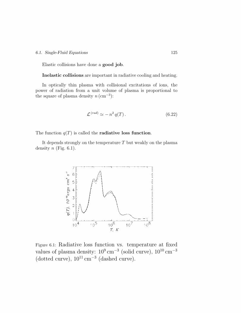
6.1. Single-Fluid Equations 125
Elastic collisions have done a good job.
Inelastic collisions are important in radiative cooling and heating.
In optically thin plasma with collisional excitations of ions, thepower of radiation from a unit volume of plasma is proportional tothe square of plasma density n (cm−3):
L (rad) ' −n2 q(T ) . (6.22)
The function q(T ) is called the radiative loss function.
It depends strongly on the temperature T but weakly on the plasmadensity n (Fig. 6.1).
Figure 6.1: Radiative loss function vs. temperature at fixedvalues of plasma density: 109 cm−3 (solid curve), 1010 cm−3
(dotted curve), 1011 cm−3 (dashed curve).
126 Chapter 6. Single-Fluid Models
6.2 Basic assumptions and the MHD equations
6.2.1 Old simplifying assumptions
As we saw above, the transfer equations determines the behavior of dif-ferent kinds of particles in a plasma once two conditions are compliedwith:
(a) many collisions occur in a characteristic time τ of a phenomenonunder consideration:
τ À τc , (6.23)
(b) the mean free path λc is significantly smaller than the dis-tance L, over which macroscopic quantities change considerably:
L À λc . (6.24)
Once these conditions are satisfied, we can close the set of transferequations, as was discussed in Sect. 4.6.
While considering the generalized Ohm’s law, other three assump-tions have been made.
The first condition can be written in the form
τ À τei , (6.25)
where τei is the electron-ion collisional time, the longest collisionalrelaxation time.
Thus the electrons and ions have comparable temperatures, ideally,the same temperature T .
Second, we neglect the electron inertia in comparison with thatof the ions.
This condition is usually written as
τ À(ω (i)
B
)−1, where ω (i)
B=
eB
mi c. (6.26)
6.2. MHD Equations 127
Thus the plasma motions have to be so slow that their frequency ω =1/τ is smaller than the lowest gyro-frequency of the particles.
The third condition,
ω (e)B
τei ¿ 1 , (6.27)
is necessary to write down Ohm’s law in the form
j = σ(E +
1
cv ×B
)+ ρ q v . (6.28)
Here v is the velocity of plasma, E and B are the electric and magneticfields in the ‘laboratory’ system of coordinates, where we measure thevelocity v.
Accordingly, the field
E v = E +1
cv ×B (6.29)
is the electric field in a frame of reference related to the plasma.
Complementary to the restriction (6.24) on the characteristic length L,we have to add the condition
L À rDH
, (6.30)
where rDH
is the Debye-Huckel radius.
Then the volume charge ρ q is small in comparison with the plasmadensity ρ.
Under the conditions listed above, we use the general hydrodynamic-type equations: the conservation laws for mass (6.4), momentum (6.5)and energy (6.17).
The general hydrodynamic-type equations have a muchwider area of applicability in astrophysics than the equationsof ordinary MHD derived below.
128 Chapter 6. Single-Fluid Models
The latter will be simpler than the equations derived above.
Therefore additional simplifying assumptions are necessary.
Let us introduce them.
6.2.2 New simplifying assumptions
First assumption:
the conductivity σ is large, the electromagnetic processes being notvery fast.
Then, in the Maxwell’s equation
rotB =4π
cj +
1
c
∂E
∂t,
we ignore the displacement current in comparison to the conductiveone.
The corresponding condition is found by evaluating the currents asfollows
1
c
E
τ¿ 4π
cj or ωE ¿ 4πσE .
Thus
ω ¿ 4πσ .(6.31)
In the same order to the small parameter ω/σ, we neglect theconvective current in comparison with the conductive current inOhm’s law.
Actually,
ρ q v ≈ v div E1
4π≈ L
τ
E
L
1
4π≈ ω
4πE ¿ σE ,
once the condition (6.31) is satisfied.
6.2. MHD Equations 129
The conductivity of astrophysical plasma is often very high (Exer-cise 5.1).
This is why condition (6.31) is satisfied up to frequencies close tooptical ones.
Neglecting the displacement current and the convectivecurrent, Maxwell’s equations and Ohm’s law result in the followingrelations:
j =c
4πrotB , (6.32)
E = − 1
cv ×B +
c
4πσrotB , (6.33)
ρ q = − 1
4πcdiv (v ×B ) , (6.34)
div B = 0 , (6.35)
∂B
∂t= rot (v ×B ) +
c2
4πσ∆B . (6.36)
Once B and v are given, the current j, the electric field E, and thevolume charge ρ q are determined by formulae (6.32)—(6.34).
Thus
the problem is reduced to finding the interaction of two vectorfields: the magnetic field B and the hydrodynamic velocityfield v.
As a consequence, the approach under discussion is known as magne-tohydrodynamics (MHD).
The corresponding equation of motion is obtained by substitutionof (6.32)–(6.34) in the equation of momentum transfer (6.5).
With the viscous forces as usually written in hydrodynamics, wehave
130 Chapter 6. Single-Fluid Models
ρdv
dt= −∇p + ρ q E− 1
4πB× rotB+
+ η ∆v +(ζ +
η
3
)∇ div v . (6.37)
Here η is the first viscosity coefficient, ζ is the second viscositycoefficient (see Landau and Lifshitz, Fluid Mechanics).
Formulae for these coefficients and the viscous forces should be de-rived from the moment equation for the pressure tensor.
∗ ∗ ∗
The second additional assumption has to be introduced now.
Treating Equation (6.37), the electric force ρ q E can be ignoredin comparison to the magnetic one if
v2 ¿ c2 , (6.38)
that is in the non-relativistic approximation.
To make certain that this is true, evaluate the electric force
ρ q E ≈ 1
4πc
vB
L
vB
c≈ B2
4π
1
L
v2
c2(6.39)
and the magnetic force
1
4π|B× rotB | ≈ B2
4π
1
L. (6.40)
Comparing (6.39) with (6.40), we see that the electric force is a factorof v2/c2 short of the magnetic one.
In a great number of astrophysical applications, the plasma veloci-ties fall far short of the speed of light.
The Sun is a good case in point.
6.2. MHD Equations 131
The largest velocities in coronal mass ejections (CMEs) do notexceed 3× 108 cm/s.
Thus,we neglect the electric force acting upon the volume charge in
comparison with the magnetic force.
However the relativistic objects like accretion disks near rotatingblack holes (Novikov and Frolov, 1989), and pulsar magnetospheresare at the other extreme.
The electric force plays a crucial role in electrodynamics of relativis-tic objects.
6.2.3 Non-relativistic MHD
With the assumptions made above (2 + 3 + 2),
the considerable simplifications have been obtained;
and now we write the following set of equations of non-relativisticMHD:
∂
∂tρ vα = − ∂
∂rβ
Π ∗αβ , (6.41)
∂B
∂t= rot (v ×B ) + νm ∆B , (6.42)
div B = 0 , (6.43)
∂ρ
∂t+ div ρv = 0 , (6.44)
∂
∂t
(ρv2
2+ ρε +
B2
8π
)= − div G , (6.45)
p = p (ρ, T ) . (6.46)
The momentum of electromagnetic field does not appear on the left-hand side of (6.41).
132 Chapter 6. Single-Fluid Models
It is negligibly small in comparison to the plasma momentum ρ vα.
This fact is a consequence of neglecting the displacement current.
On the right-hand side of (6.41), the asterisk refers to the totalmomentum flux tensor Π ∗
αβ, which equals
Π ∗αβ = ρ vαvβ +
(p δαβ − σv
αβ
)+
+1
4π
(B2
2δαβ −BαBβ
). (6.47)
In Equation (6.42)
νm =c2
4πσ(6.48)
is the magnetic viscosity.
It plays the same role as the kinematic viscosity ν = η/ρ in theequation of motion.
The vector G is defined as the energy flux
Gα = ρ vα
(v2
2+ w
)+
1
4π[B× (v ×B ) ]α−
− νm
4π(B× rotB )α − σv
αβ vβ − κ∇α T . (6.49)
The Poynting vector as a part in (6.49) is
GP
=1
4πB× (v ×B ) − νm
4πB× rot B . (6.50)
The energy flux due to friction is written as the contraction of thevelocity vector v and the viscous stress tensor σv
αβ .
6.2. MHD Equations 133
6.2.4 Energy conservation
The non-relativistic MHD equations are frequently used to model solarflares, eruptive prominences, etc.
A goal of such studies is to deduce how energy of magnetic fieldis stored and then suddenly released to drive these phenomena.
However
most models use a simple energy equation,
the discussion often centers on the over-simplified interpretationor
just comparison of magnetic field structure in the models withcorresponding features observed in emission.
With new capabilities to study X-ray and EUV emission from Hin-ode and complementary observations from SOHO, RHESSI and othersatellites, the models advance to more quantitative results.
We have to develop the MHD models that include radiative lossesand other dissipative processes, the energy transport by anisotropicheat conduction.
The equation of state (6.46) can be rewritten in other thermody-namic variables.
In order to do this, we have to make use of the thermodynamicidentities
dε = T ds +p
ρ2dρ and dw = T ds +
1
ρdp .
Here s is the entropy per unit mass.
We transform the energy conservation law (6.45) from the divergentform to the hydrodynamic one:
ρ Tds
dt=
νm
4π(rot B)2 + σv
αβ
∂vα
∂rβ
+
+ div κ∇T + L (rad) (r, t) . (6.51)
134 Chapter 6. Single-Fluid Models
Thus
the heat abundance change dQ = ρ T ds in a moving elementof unit volume is a sum of the Joule and viscous heating,conductive heat redistribution and radiative cooling.
6.2.5 Relativistic magnetohydrodynamics
Relativistic MHD models are of considerable interest in several areasof modern astrophysics.
The theory of gravitational collapse and models of supernova ex-plosions are based on relativistic hydrodynamics for a star.
The effects of deviations from spherical symmetry due to magneticfield require the use of relativistic MHD models.
Relativistic hydrodynamics is presumably applied to the so-calledquark-gluon plasma which is the primordial state of hadronic matterin the Universe.
When the medium interacts electromagnetically and is highly con-ducting, the simplest description is in terms of relativistic MHD.
From the mathematical viewpoint, the relativistic MHD was mainlytreated in the framework of general relativity.
This means that the MHD equations were studied in conjunctionwith Einstein’s equations.
Lichnerowicz (1967) has made a thorough and deep investigation ofthe initial value problem.
In many applications, however, one neglects the gravitational fieldgenerated by the conducting medium in comparison with the back-ground gravitational field
as well as
in many cases one simply uses special relativity.
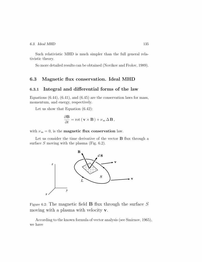
6.3. Ideal MHD 135
Such relativistic MHD is much simpler than the full general rela-tivistic theory.
So more detailed results can be obtained (Novikov and Frolov, 1989).
6.3 Magnetic flux conservation. Ideal MHD
6.3.1 Integral and differential forms of the law
Equations (6.44), (6.41), and (6.45) are the conservation laws for mass,momentum, and energy, respectively.
Let us show that Equation (6.42):
∂B
∂t= rot (v ×B ) + νm ∆B ,
with νm = 0, is the magnetic flux conservation law.
Let us consider the time derivative of the vector B flux through asurface S moving with the plasma (Fig. 6.2).
B
S
SL
d
v
v
xy
z
Figure 6.2: The magnetic field B flux through the surface Smoving with a plasma with velocity v.
According to the known formula of vector analysis (see Smirnov, 1965),we have
136 Chapter 6. Single-Fluid Models
d
dt
∫
S
B · dS =∫
S
(∂ B
∂t+ v div B + rot (B× v )
)· dS .
Since div B = 0,
d
dt
∫
S
B · dS =∫
S
(∂ B
∂t− rot (v ×B )
)· dS ,
or, making use of Equation (6.42),
d
dt
∫
S
B · dS = νm
∫
S
∆B · dS .
(6.52)
Thus, if we cannot neglect magnetic viscosity νm, then
the change rate of magnetic flux through a surface mov-ing together with a conducting plasma is proportional tothe magnetic viscosity.
The right-hand side of (6.52) can be rewritten with the help of theStokes theorem:
d
dt
∫
S
B · dS = − νm
∮
L
rot B · d l .
Here L is the ‘liquid contour’ bounding the surface S.
By using equation
j =c
4πrotB ,
we haved
dt
∫
S
B · dS = − c
σ
∮
L
j · d l .
(6.53)
6.3. Ideal MHD 137
The change rate of flux is proportional to resistivity σ−1 of the plasma.
Equation (6.53) is equivalent to the differential Equation (6.42) andpresents an integral form of the magnetic flux conservation law.
The magnetic flux through any surface moving with theplasma is conserved, once the electric resistivity σ−1 can beignored.
When is it possible to neglect resistivity of plasma?
The relative role of a dissipation process can be evaluated as follows.
Let us pass on to the dimensionless variables
r∗ =r
L, t∗ =
t
τ, v∗ =
v
v, B∗ =
B
B0
.
On substituting them in (6.42) we obtain
B0
τ
∂ B∗
∂t∗=
vB0
Lrot∗ (v∗ ×B∗ ) + νm
B0
L2∆∗B∗ .
Now we normalize this equation with respect to its left-hand side, i.e.
∂ B∗
∂t∗=
vτ
Lrot∗ (v∗ ×B∗ ) +
νmτ
L2∆∗B∗ .
This dimensionless equation contains two dimensionless param-eters.
The first one,
δ =vτ
L,
will be discussed later on.
Here, for simplicity, we assume δ = 1.
The second parameter,
138 Chapter 6. Single-Fluid Models
Rem =L2
νm τ=
vL
νm
,
(6.54)
is termed the magnetic Reynolds number, by analogy with the hy-drodynamic Reynolds number
Re =vL
ν.
Omitting the asterisk, we write the dimensionless equation
∂ B
∂t= rot (v ×B ) +
1
Rem
∆B . (6.55)
The larger the magnetic Reynolds number, the smaller therole played by magnetic viscosity.
So the magnetic Reynolds number is the measure of a relative impor-tance of resistivity.
If
Rem À 1 ,
we neglect the plasma resistivity and, as a consequence, magneticfield diffusion and dissipation.
On the contrary, in laboratory, e.g., in devices for studying recon-nection, because of a small value L2, the magnetic Reynolds number isusually not large:
Rem ∼ 1− 3 .
In this case, the resistivity has a dominant role, and dissipation isimportant.
6.3. Ideal MHD 139
6.3.2 The ideal MHD
Under astrophysical conditions, owing to the low resistivity of plasmaand the enormously large length scales, the magnetic Reynolds num-ber is usually huge:
Rem > 1010
(e.g., Exercise 6.1).
Thus, in a great number of problems, it is sufficient to consider amedium with infinite conductivity:
Rem À 1 .
Furthermore the usual Reynolds number can be also large (see, however,Exercise 6.2):
Re À 1 .
Let us also assume the heat exchange to be of minor importance.
This assumption is not universally true either.
Sometimes the thermal conductivity is so effective that an astro-physical plasma must be considered as isothermal, rather than adia-batic.
However, conventionally,
while treating the ‘ideal medium’, all dissipative coefficientsas well as the thermal conductivity are set equal to zero:
νm = 0 , η = ζ = 0 , κ = 0 .
The complete set of the ideal MHD equations has two equivalentforms.
The first one is the transfer equations:
140 Chapter 6. Single-Fluid Models
∂v
∂t+ (v · ∇)v = −∇p
ρ− 1
4πρB× rot B ,
∂ B
∂t= rot (v ×B) , div B = 0 , (6.56)
∂ρ
∂t+ div ρv = 0 ,
∂s
∂t+ (v · ∇) s = 0 ,
p = p (ρ, s) .
The divergent form corresponds to the conservation laws forenergy, momentum, mass and magnetic flux:
∂
∂t
(ρv2
2+ ρε +
B2
8π
)= − div G , (6.57)
∂
∂tρ vα = − ∂
∂rβ
Π ∗αβ , (6.58)
∂ρ
∂t= − div ρv , (6.59)
∂ B
∂t= rot (v ×B ) , (6.60)
div B = 0 , (6.61)
p = p (ρ, s) . (6.62)
Here the energy flux and the momentum flux tensor are
G = ρv
(v2
2+ w
)+
1
4π
(B2 v − (B · v)B
)(6.63)
and
Π ∗αβ = p δαβ + ρ vαvβ +
1
4π
(B2
2δαβ −BαBβ
). (6.64)
6.3. Ideal MHD 141
6.3.3 The ‘frozen field’ theorem
The magnetic flux conservation law (6.60) written in the integral form
d
dt
∫
S
B · dS = 0
allows us to represent the magnetic field as a set of field lines attachedto the medium, as if they were ‘frozen into’ it.
For this reason, (6.60) is referred to as the ‘freezing-in’ equation.
The “frozen field” theorem can be formulated as follows.
In the ideally conducting medium, the field lines move to-gether with the plasma. A medium motion conserves notonly the magnetic flux but each of the field lines as well.
Let us imagine a thin tube of field lines (Fig. 6.3).
There is no magnetic flux through any part of the surface formedby the boundary field lines that intersect the closed curve L.
Hence, the “fluid particles” that are initially in the same fluxtube must remain in the flux tube.
In ideal MHD flows, magnetic field lines are therefore material-ized and are unbreakable because the flux tube links the same fluidparticles.
As a result its topology cannot change.
Fluid particles which are not initially on a common field line cannotbecome linked by one later on.
This general topological constraint restricts the idealMHD motions, forbidding a lot of motions that would oth-erwise appear.
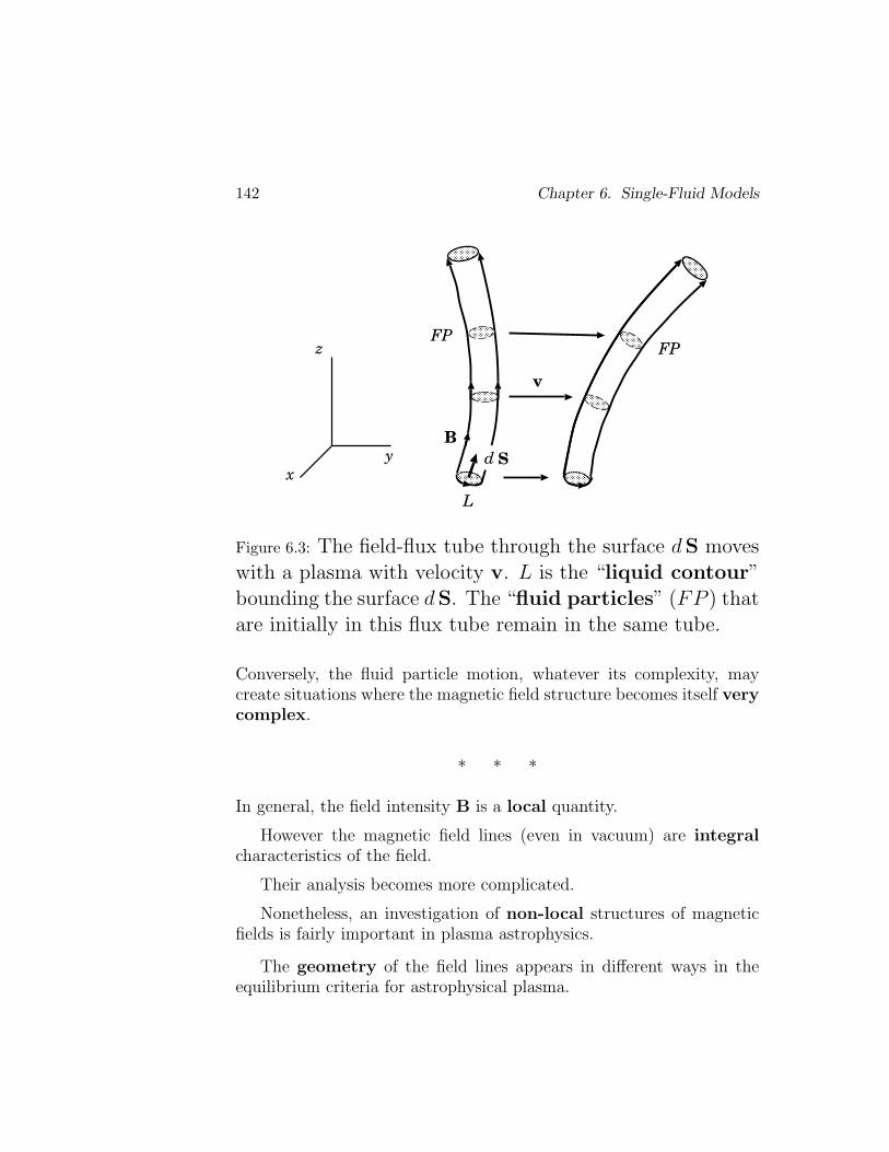
142 Chapter 6. Single-Fluid Models
B
L
v
xy
z
Sd
FPFP
Figure 6.3: The field-flux tube through the surface dS moveswith a plasma with velocity v. L is the “liquid contour”bounding the surface dS. The “fluid particles” (FP ) thatare initially in this flux tube remain in the same tube.
Conversely, the fluid particle motion, whatever its complexity, maycreate situations where the magnetic field structure becomes itself verycomplex.
∗ ∗ ∗
In general, the field intensity B is a local quantity.
However the magnetic field lines (even in vacuum) are integralcharacteristics of the field.
Their analysis becomes more complicated.
Nonetheless, an investigation of non-local structures of magneticfields is fairly important in plasma astrophysics.
The geometry of the field lines appears in different ways in theequilibrium criteria for astrophysical plasma.
6.4. Magnetic Reconnection 143
Much depends on whether the field lines are concave or convex,on the so-called specific volume of magnetic flux tubes.
However even more depends on the presence of X-type points, aswell as on other topological characteristics, e.g. the global magnetichelicity.
6.4 Magnetic reconnection
Reconnection of magnetic field lines is the physical process which in-volves a breakdown of the “frozen field” theorem.
The effects of electric resistivity, normally negligible in thelarge, become locally dominant
with dramatic consequences in the large-scale plasma flows and mag-netic field configuration.
Reconnection changes topology of magnetic field.
The origin of the concept of reconnection lies in an attempt by Gio-vanelli (1946) to explain solar flares.
Reconnection is the means by which energy stored in magneticfields is released rapidly to produce such phenomena as solar flaresand magnetospheric substorms.
Furthermore, reconnection plays important roles in many areas ofastrophysics.
Depending on complexity of fields and conditions, reconnectioncan occur over an extended region in space or can be “patchy” and“unpredictable”.
For example, in the Earth’s magnetosphere the reconnecting cur-rent layers (RCLs) are formed by the interaction between the solarwind and the geomagnetic field.
Such RCLs have finite extents, and their boundary conditionsoften change rapidly.
On the contrary,
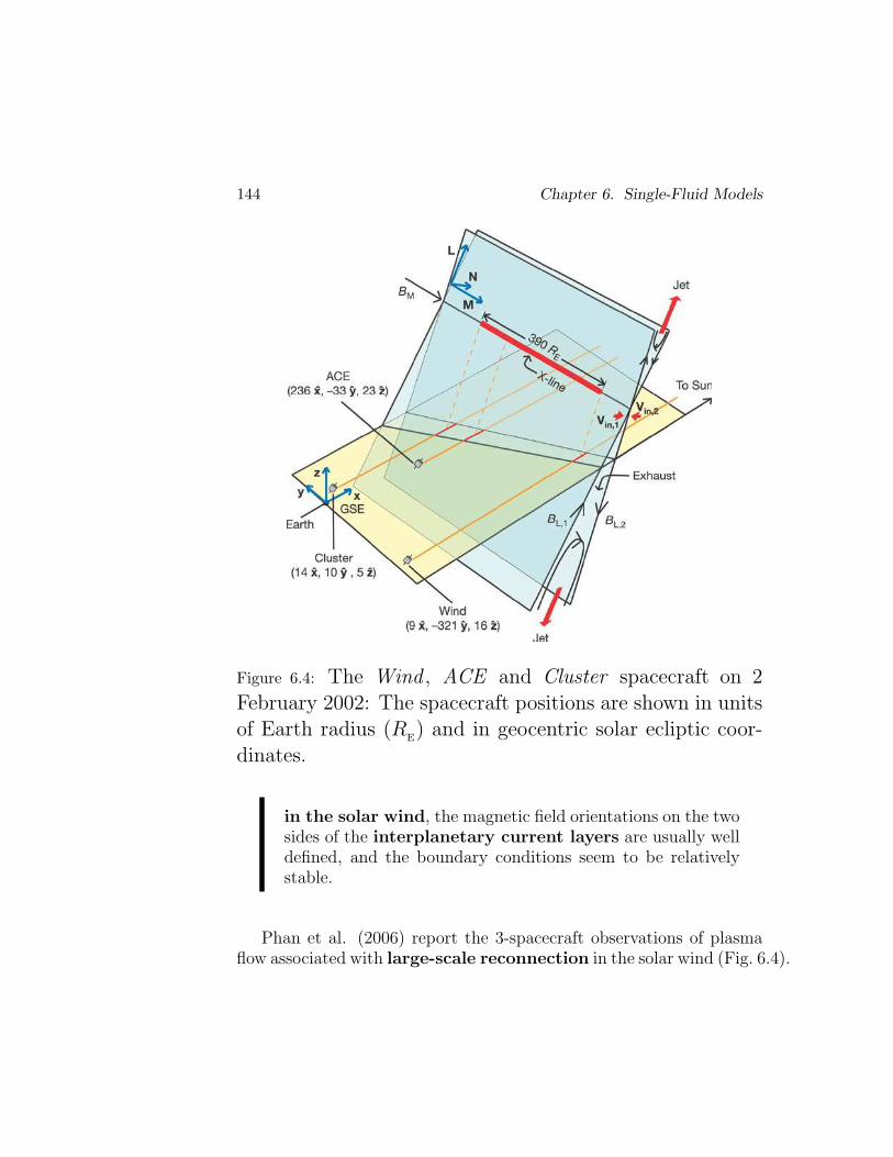
144 Chapter 6. Single-Fluid Models
Figure 6.4: The Wind , ACE and Cluster spacecraft on 2February 2002: The spacecraft positions are shown in unitsof Earth radius (R
E) and in geocentric solar ecliptic coor-
dinates.
in the solar wind, the magnetic field orientations on the twosides of the interplanetary current layers are usually welldefined, and the boundary conditions seem to be relativelystable.
Phan et al. (2006) report the 3-spacecraft observations of plasmaflow associated with large-scale reconnection in the solar wind (Fig. 6.4).
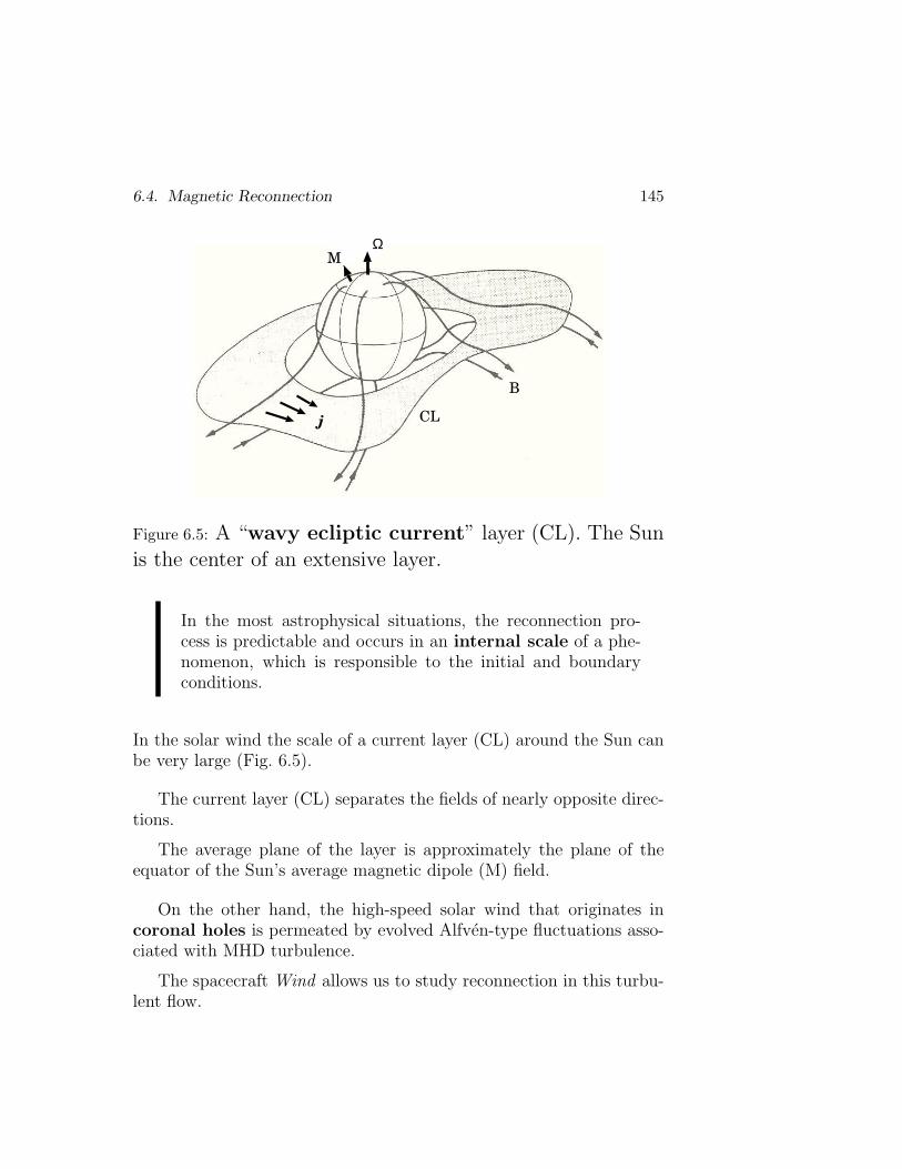
6.4. Magnetic Reconnection 145
j
B
CL
ΩM
Figure 6.5: A “wavy ecliptic current” layer (CL). The Sunis the center of an extensive layer.
In the most astrophysical situations, the reconnection pro-cess is predictable and occurs in an internal scale of a phe-nomenon, which is responsible to the initial and boundaryconditions.
In the solar wind the scale of a current layer (CL) around the Sun canbe very large (Fig. 6.5).
The current layer (CL) separates the fields of nearly opposite direc-tions.
The average plane of the layer is approximately the plane of theequator of the Sun’s average magnetic dipole (M) field.
On the other hand, the high-speed solar wind that originates incoronal holes is permeated by evolved Alfven-type fluctuations asso-ciated with MHD turbulence.
The spacecraft Wind allows us to study reconnection in this turbu-lent flow.
146 Chapter 6. Single-Fluid Models
The Wind observations demonstrate that
reconnection is one way in which the solar wind turbulenceis dissipated and the high-speed wind is heated far from theSun.
In the solar wind, the kinetic and thermal energies of plasma exceedthe magnetic energy.
We neglect the magnetic force as compared to the inertia force ofmoving plasma and its pressure gradient.
We call such a process as reconnection in a weak magnetic field.
Another example of this phenomenon is the photospheric reconnec-tion.
Reconnection in a strong magnetic field is a fundamental feature ofastrophysical plasmas like the solar corona.
Such reconnection explains an accumulation of magnetic energy anda sudden release of this energy, a flare.
This phenomenon is accompanied by fast ejections of plasma, pow-erful flows of heat and hard electromagnetic radiation, by accelerationof particles.
6.5 Practice: Exercises and Answers
Exercise 6.1. Estimate the magnetic Reynolds number in the solarcorona.
Answer.
Taking characteristic values of the parallel conductivity as estimatedin Exercise 5.1:
σ ‖ = σ ∼ 1016 − 1017 s−1 ,
we obtain
6.5. Practice: Exercises and Answers 147
Rem =vL
νm
∼ 1011 − 1012 , (6.65)
if the length and velocity, L ∼ 104 km and v ∼ 10 km s−1.
Exercise 6.2. Show that
in the solar corona, usual viscosity of plasma can be a muchmore important dissipative mechanism than electric resistiv-ity.
Answer.
The characteristic value of kinematic viscosity
ν =η
ρ≈ 3× 1015 cm2 s−1.
Here Tp ≈ 2 × 10⁶ K and np ≈ ne ≈ 2 × 108 cm−3 were taken as thetypical proton temperature and density.
If the length and velocity, L ∼ 109 cm and v ∼ 106 cm s−1, thenthe ordinary Reynolds number
Re =vL
ν∼ 0.3 . (6.66)
Thus
Rem À Re .

148 Chapter 6. Single-Fluid Models
Chapter 7
MHD in Astrophysics
MHD is appropriate for many phenomena in astrophysicalplasma, that take place on a relatively large scale.
The non-relativistic MHD is applied to dynamo theory, flowsin the solar atmosphere, flares, coronal heating, solar andstellar winds.
Relativistic MHD describes well accretion disks near rela-tivistic objects, and relativistic jets.
7.1 The main approximations in ideal MHD
7.1.1 Dimensionless equations
The equations of MHD constitute a set of nonlinear differential equa-tions in partial derivatives.
The order of the set is rather high, and its structure is complicated.
To formulate a problem, we have to know the initial and bound-ary conditions admissible by this set of equations.
To do this, in turn, we have to know the type of equations, in thesense adopted in mathematical physics.
To formulate a problem, we usually use one or another approxima-tion, which makes it possible to point up and isolate the main effect.
149
150 Chapter 7. MHD in Astrophysics
For instance, if the magnetic Reynolds number is small, aplasma moves comparatively easily with respect to magnetic field.
This is the case in laboratory and technical devices.
The opposite approximation is that of large magnetic Reynoldsnumbers, when the magnetic field ‘freezing in’ takes place in plasma.
This approximation is quite characteristic of the astrophysical plasma.
How can we isolate the main effect in a phenomenon and correctlyformulate the problem? – From the above examples, the following rulesuggests itself:
take the dimensional parameters of a phenomenon, combinethem into dimensionless combinations, calculate their values,and use a corresponding approximation in the dimensionlessequations.
Such an approach is effective in hydrodynamics.
Let us start with the ideal MHD equations:
∂v
∂t+ (v · ∇)v = −∇p
ρ− 1
4πρB× rot B , (7.1)
∂ B
∂t= rot (v ×B) , (7.2)
∂ρ
∂t+ div ρv = 0 , (7.3)
∂s
∂t+ (v · ∇) s = 0 , (7.4)
div B = 0 , (7.5)
p = p (ρ, s) . (7.6)
Let the quantities
7.1. Main Approximations in Ideal MHD 151
L, τ, v, ρ0 , p0 , s0 , B0
be the characteristic values of length, time, velocity, density, pressure,entropy and field strength, respectively.
Rewrite Equations (7.1)–(7.6) in the dimensionless variables
r∗ =r
L, t∗ =
t
τ, . . . B∗ =
B
B0
.
Omitting the asterisk, we obtain the equations in dimensionless vari-ables:
ε2
1
δ
∂v
∂t+ (v · ∇)v
= − γ2 ∇p
ρ− 1
ρB× rot B , (7.7)
∂ B
∂t= δ rot (v ×B) , (7.8)
∂ρ
∂t+ δ div ρv = 0 , (7.9)
∂s
∂t+ δ (v · ∇) s = 0 , (7.10)
div B = 0 , (7.11)
p = p (ρ, s) . (7.12)
Here
δ =vτ
L, ε2 =
v2
V 2A
, γ2 =p0
ρ0V 2A
(7.13)
are three dimensionless parameters;
VA
=B0√4πρ0
(7.14)
152 Chapter 7. MHD in Astrophysics
is the characteristic value of the Alfven speed (see Exercise 7.1).
If the gravitational force is taken into account, Equation (7.7) con-tains another dimensionless parameter,
gL/V 2A
,
where g is the gravitational acceleration.
The analysis of these parameters allows us to separate the approxi-mations which are possible in the ideal MHD.
7.1.2 Weak magnetic fields in astrophysical plasma
We begin with the assumption that
ε2 À 1 and γ2 À 1 . (7.15)
As is seen from Equation (7.7), in the zero-order approximation relativeto the small parameters
ε−2 and γ−2 ,
we neglect the magnetic force as compared to the inertia force andthe pressure gradient.
In subsequent approximations, the magnetic effects are treated assmall corrections to the hydrodynamic ones.
A lot of problems of plasma astrophysics are solved in this approx-imation, termed the weak magnetic field approximation.
Among the simplest of them are the ones concerning the weak field’sinfluence on hydrostatic equilibrium.
An example is the problem of the influence of magnetic field on theequilibrium of a self-gravitating plasma ball (a star, the magnetoid ofquasar’s kernel etc.).
Some other problems are in fact analogous to the mentioned ones.
They are called kinematic problems, since
7.1. Main Approximations in Ideal MHD 153
they treat the influence of a given plasma flow on magneticfield; the reverse influence is considered to be negligible.
Such problems are reduced to finding the magnetic field resulting fromthe known velocity field.
An example is the magnetic field amplification and support by sta-tionary plasma flows (magnetic dynamo).
The simplest example is the magnetic field amplification by differ-ential rotation.
A leading candidate to explain the origin of large-scale magneticfields in astrophysical plasma is the turbulent dynamo theory.
7.1.3 Strong magnetic fields in plasma
The opposite approximation – that of the strong field – reflects thespecificity of MHD to a greater extent.
This approximation is valid when the magnetic force
Fm = − 1
4πB× rot B (7.16)
dominates all the others (inertia force, pressure gradient, etc.).
In Equation (7.7), the magnetic field is a strong one if
ε2 ¿ 1 and γ2 ¿ 1 , (7.17)
i.e. the magnetic energy density greatly exceeds that of the kinetic andthermal energies:
B 20
8πÀ ρ0v
2
2and
B 20
8πÀ 2n0kB
T0 .
From Equation (7.7) it follows that, in the zeroth order with respectto the small parameters (7.17), the magnetic field is force-free:
154 Chapter 7. MHD in Astrophysics
B× rot B = 0 . (7.18)
This conclusion is quite natural:
if the magnetic force dominates all the others, the magneticfield must balance itself in the region under consideration.
Condition (7.18) means that electric currents flow parallel to magneticfield lines.
If, in addition, electric currents are absent in some region, then thestrong field is simply potential:
rot B = 0 , B = ∇Ψ , ∆Ψ = 0 . (7.19)
Let us consider the first order in the small parameters (7.17).
If they are not equally significant, there are two possibilities.
(a) We suppose, at first, that
ε2 ¿ γ2 ¿ 1 . (7.20)
Then we neglect the inertia force in Equation (7.7) as compared to thepressure gradient.
Decomposing the magnetic force into a magnetic tension forceand a magnetic pressure gradient,
Fm = − 1
4πB× rot B =
1
4π(B · ∇)B−∇ B2
8π, (7.21)
we obtain the following dimensionless equation:
(B · ∇)B = ∇(
B2
2+ γ2p
). (7.22)
Owing to the gas pressure gradient, the magnetic field differs fromthe force-free one:
7.1. Main Approximations in Ideal MHD 155
the magnetic tension force (B·∇)B/4π must balance not onlythe magnetic pressure gradient but that of the gas pressureas well.
Obviously the effect is proportional to the small parameter γ2.
This approximation is naturally called the magnetostatics sincev = 0.
It works in regions of a strong magnetic field where the gas pressuregradients are large, e.g., in coronal loops and reconnecting currentlayers in the solar corona.
(b) The inertia force also causes the magnetic field to deviatefrom the force-free one:
ε2
1
δ
∂v
∂t+ (v · ∇)v
= − 1
ρB× rot B . (7.23)
Here we ignored the pressure gradient as compared with the inertiaforce.
This is the case
γ2 ¿ ε2 ¿ 1 . (7.24)
The approximation corresponding (7.24) is termed the approximationof strong field and cold plasma.
The main applications of this approximation are the solar atmo-sphere and the Earth’s magnetosphere.
Both objects are well studied from the observational viewpoint.
So we can proceed with confidence from qualitative interpreta-tion to the construction of quantitative models.
The presence of a strong field and a rarefied plasma is common forboth phenomena.
156 Chapter 7. MHD in Astrophysics
A sufficiently strong magnetic field easily moves a compar-atively rarefied plasma in many non-stationary phenomena inspace.
Some astrophysical applications will be discussed in the followingtwo Sections.
∗ ∗ ∗
In closing, let us consider the dimensionless parameter
δ = vτ/L .
It characterizes the relative role ofthe local ∂/∂tand transport (v · ∇)terms in the substantial derivative
d
dt=
1
δ
∂
∂t+ (v · ∇) .
If δ À 1, the flow can be considered to be stationary
ε2 (v · ∇)v = − 1
ρB× rot B . (7.25)
If δ ¿ 1, the transport term (v · ∇) can be ignored, and the equationof motion takes the form
ε2 ∂v
∂t= − 1
ρB× rot B , (7.26)
other equations becoming linear.
This case corresponds to small small perturbations.
If need be, the right-hand side of Equation (7.26) can be linearizedtoo.
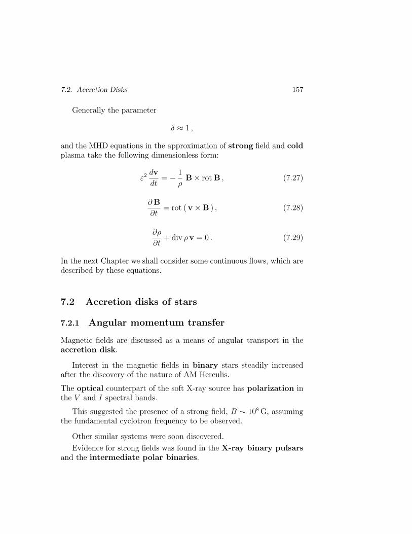
7.2. Accretion Disks 157
Generally the parameter
δ ≈ 1 ,
and the MHD equations in the approximation of strong field and coldplasma take the following dimensionless form:
ε2 dv
dt= − 1
ρB× rot B , (7.27)
∂ B
∂t= rot (v ×B ) , (7.28)
∂ρ
∂t+ div ρv = 0 . (7.29)
In the next Chapter we shall consider some continuous flows, which aredescribed by these equations.
7.2 Accretion disks of stars
7.2.1 Angular momentum transfer
Magnetic fields are discussed as a means of angular transport in theaccretion disk.
Interest in the magnetic fields in binary stars steadily increasedafter the discovery of the nature of AM Herculis.
The optical counterpart of the soft X-ray source has polarization inthe V and I spectral bands.
This suggested the presence of a strong field, B ∼ 108 G, assumingthe fundamental cyclotron frequency to be observed.
Other similar systems were soon discovered.
Evidence for strong fields was found in the X-ray binary pulsarsand the intermediate polar binaries.
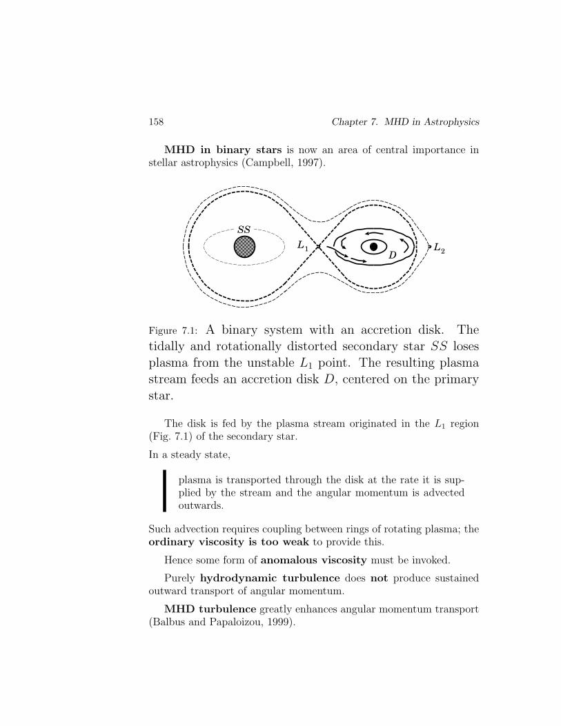
158 Chapter 7. MHD in Astrophysics
MHD in binary stars is now an area of central importance instellar astrophysics (Campbell, 1997).
D
L1
SS
L2
Figure 7.1: A binary system with an accretion disk. Thetidally and rotationally distorted secondary star SS losesplasma from the unstable L1 point. The resulting plasmastream feeds an accretion disk D, centered on the primarystar.
The disk is fed by the plasma stream originated in the L1 region(Fig. 7.1) of the secondary star.
In a steady state,
plasma is transported through the disk at the rate it is sup-plied by the stream and the angular momentum is advectedoutwards.
Such advection requires coupling between rings of rotating plasma; theordinary viscosity is too weak to provide this.
Hence some form of anomalous viscosity must be invoked.
Purely hydrodynamic turbulence does not produce sustainedoutward transport of angular momentum.
MHD turbulence greatly enhances angular momentum transport(Balbus and Papaloizou, 1999).
7.2. Accretion Disks 159
Turbulent viscous and magnetic stresses cause radial ad-vection of the angular momentum via the azimuthal forces.
7.2.2 Accretion in cataclysmic variables
Cataclysmic variables (CVs) are binary systems composed of a whitedwarf (primary star) and a late-type, main-sequence companion (sec-ondary star).
The way this plasma falls towards the primary depends on the in-tensity of a magnetic field of the white dwarf.
The strong field (B >∼ 107 G) may entirely dominate the accretionflow.
The magnetic field is strong enough to synchronize the white dwarfrotation (spin) with the orbital period.
No disk is formed.
Instead, the field channels accretion towards its polar regions.
Such synchronous systems are known as AM Herculis binaries orpolars.
The intermediate (B ∼ 2− 8× 10⁶ G) field primary stars harbormagnetically truncated accretion disks which extend until magneticpressure begins to dominate.
Presumably the plasma is finally accreted onto the magnetic polesof the white dwarf.
The asynchronous systems are known as DQ Herculis binaries orintermediate polars (IPs).
The accretion geometry strongly influences the emission propertiesat all wavelengths and its variability.
The knowledge of the behavior in all energy domains can allow oneto locate the different accreting regions.
160 Chapter 7. MHD in Astrophysics
The white dwarf LHS 2534 offers the first empirical data of theZeeman effect on neutral Na, Mg, and both ionized and neutral Ca.
The Na I splitting results in a field strength estimate of 1.92×10⁶ G.
7.2.3 Accretion disks near black holes
In the binary stars discussed above, there is an abundance of evi-dence for accretion disks:
(a) double-peaked emission lines,
(b) eclipses of an extended light source centered on the primary,
(c) eclipses of the secondary star by the disk.
The case of accretion disks in active galactic nuclei (AGN) is lessclear.
Nonetheless the disk accretion onto a super-massive black holeis the commonly accepted model for these objects.
As the plasma accretes in the gravitational field of the central mass,magnetic field lines are convected inwards, amplified and finally de-posited on the horizon of the black hole.
As long as a magnetic field is confined by the disk, a differentialrotation causes the field to wrap up tightly, becoming highly shearedand predominantly azimuthal in orientation.
A dynamo in the disk may be responsible for the maintenance andamplification of the magnetic field.
In the standard model of an accretion disk (Shakura and Sunya-ev, 1973; Novikov and Thorne, 1973), the gravitational energy is locallyradiated from the optically thin disk.
However the expected power far exceeds the observed lumi-nosity.
There are two possible explanations:
(a) the accretion occurs at extremely low rates, or
7.2. Accretion Disks 161
(b) the accretion occurs at low radiative efficiency.
Advection results in a structure different from the standard model.
The advection process physically means that
the energy generated via viscous dissipation is restored as en-tropy of the accreting plasma flow rather than being radi-ated.
An optically thin advection-dominated accretion flow (ADAF)seemed to be a model that can reproduce the observed spectra of blackhole systems such as AGN and Galactic black hole candidates.
7.2.4 Flares in accretion disk coronae
Following the launch of several X-ray satellites, astrophysicists havetried to observe and analyze the variations of high energy flux fromblack hole candidates.
It has appeared that
there are many relationships between flares in the solarcorona and ‘X-ray shots’ in accretion disks.
For example, the peak interval distribution of Cyg X-1 shows that theoccurrence frequency of large X-ray shots is reduced.
A second large shot does not occur soon after a previous large shot.
This suggests the existence of energy-accumulation structures,such as non-potential magnetic fields in the solar corona.
It is likely that accretion disks have a corona.
Galeev et al. (1979) suggested that the corona is confined in strongmagnetic loops which have buoyantly emerged from the disk.
Magnetic reconnection of buoyant fields in the lower den-sity surface regions may supply the energy source for a hotcorona.
162 Chapter 7. MHD in Astrophysics
The existence of a disk corona with a strong field raises the possibilityof a wind flow similar to the solar wind.
This would result in angular momentum transport away fromthe disk, which could have some influence on the inflow.
Another feature is the possibility of a flare energy release similarto solar flares.
When a plasma in the disk corona is optically thin and has adominant magnetic pressure, the circumstances are similar to thesolar corona.
Therefore
it is possible to imagine some similarity between the mecha-nisms of solar flares and X-ray shots in accretion disk coronae.
Besides the effect of heating the the disk corona, reconnection isable to accelerate particles to high energies.
Some geometrical and physical properties of the flares in disk coro-nae can be inferred from X-ray observations of Galactic black hole can-didates.
7.3 Astrophysical jets
7.3.1 Jets near black holes
Jet-like phenomena, including relativistic jets, are observed on a widerange of scales in accretion disk systems.
AGN show extremely energetic outflows extending beyond theouter edge of a galaxy in the form of strongly collimated jets.
There is evidence that magnetic forces are involved in thedriving mechanism and that the magnetic fields also provide thecollimation of relativistic flows.
7.3. Astrophysical Jets 163
Rotating black holes are thought to be the prime-mover in centersof galaxies.
The gravitational field of rotating black holes is more complexthan that of non-rotating ones.
The weak-gravity (far from the hole) low-velocity coordinate ac-celeration of uncharged particle
d2r
dt2= g +
dr
dt×H gr . (7.30)
This looks like the Lorentz force with the electric field E replaced byg, the magnetic field B replaced by the vector
H gr = rot A gr ,
and the electric charge e replaced by the particle mass m.
These analogies lie behind the words “gravitoelectric” and “gravito-magnetic” to describe the gravitational acceleration field g and todescribe the “shift function” Agr (Exercise 7.6).
Thus, far from the horizon, the gravitational acceleration
g = −M
r2er (7.31)
is the radial Newtonian acceleration, andthe gravitomagnetic field
Hgr = 2J− 3 (J · er) er
r3(7.32)
is a dipole field.
The role of dipole moment is played by the hole’s angular momen-tum
J =∫
( r× ρmv) dV .
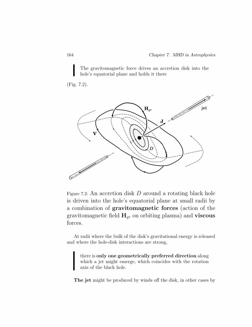
164 Chapter 7. MHD in Astrophysics
The gravitomagnetic force drives an accretion disk into thehole’s equatorial plane and holds it there
(Fig. 7.2).
H
J
gr
D
jet
V
Figure 7.2: An accretion disk D around a rotating black holeis driven into the hole’s equatorial plane at small radii bya combination of gravitomagnetic forces (action of thegravitomagnetic field Hgr on orbiting plasma) and viscousforces.
At radii where the bulk of the disk’s gravitational energy is releasedand where the hole-disk interactions are strong,
there is only one geometrically preferred direction alongwhich a jet might emerge, which coincides with the rotationaxis of the black hole.
The jet might be produced by winds off the disk, in other cases by
7.3. Astrophysical Jets 165
electrodynamic acceleration of the disk, and in others by currents inthe hole’s magnetosphere.
However whatever the mechanism, the jet presumably is locked tothe hole’s rotation axis.
The black hole acts as a gyroscope to keep the jet aligned.
It is very difficult to torque a black hole.
The fact accounts for the constancy of the observed jet directionsover length scales as great as millions of light years and thus overtime scales of millions of years or longer.
∗ ∗ ∗
In the highly-conducting medium, the gravitomagnetic force cou-ples with electromagnetic fields over Maxwell’s equations.
This effect has interesting consequences for the magnetic fields ad-vected towards the black hole.
It leads to a gravitomagnetic dynamo which amplifies any seedfield near a rotating compact object.
This process builds up the dipolar magnetic structures whichmay be behind the bipolar outflows seen as relativistic jets.
7.3.2 Relativistic jets from disk coronae
Relativistic jets are produced perpendicular to the accretion disk plane(Fig. 7.2) around a super-massive black hole in an AGN.
The shock of the jets on intergalactic media is considered as beingable to accelerate particles up to the highest energies, say 1020 eV forcosmic rays.
This hypothesis need, however, to be completed by some necessaryingradients since such powerful galaxies are rare objects.
166 Chapter 7. MHD in Astrophysics
The relativistic jets may be powered by acceleration of protonsin a corona above an accretion disk.
The acceleration arises as a consequence of the shearing motion ofthe magnetic field lines in the corona, that are anchored in the under-lying Keplerian disk.
Particle acceleration in the corona leads to the development of apressure-driven wind.
It passes through a critical point and subsequently transforms intoa relativistic jet at large distances from the black hole.
7.4 Practice: Exercises and Answers
Exercise 7.1. Evaluate the Alfven speed in the solar corona above alarge sunspot.
Answer.
From definition we find
VA≈ 2.18× 10¹¹ B√
n, cm s−1 . (7.33)
Above a sunspot B ≈ 3000 G, n ≈ 2× 108 cm−3 .
Thus (7.33) gives unacceptably high values:
VA≈ 5× 1010 cm s−1 > c .
This means that
in a strong magnetic field and low density plasma, the Alfvenwaves propagate with velocities approaching the light speed c .
So the non-relativistic formula (7.33) has to be corrected by a rela-tivistic factor:
7.4. Practice: Exercises and Answers 167
V relA
=B√4πρ
1√1 + B2/4πρc2
, (7.34)
which agrees with (7.14) if B2 ¿ 4πρc2.
Therefore the relativistic Alfven wave speed is always smaller than thelight speed.
For values of the magnetic field and plasma density mentioned above,
V relA
≈ 2× 1010 cm s−1.
Exercise 7.2. Discuss properties of the Lorentz force in terms of theMaxwellian stress tensor (6.11).
Exercise 7.3. Show that the magnetic tension force is directedto the local centre of curvature.
Exercise 7.4. For the conditions in the corona, used in Exercise 7.1,estimate the parameter γ2.
Answer.
Substitute p0 = 2n0kBT0 in definition (7.13):
For the temperature T0 ≈ 2×10⁶ K and magnetic field B0 ≈ 3000 G
γ2 ∼ 10−7 .
Exercise 7.5. By using formula (6.63) for the energy flux in idealMHD, find the magnetic energy influx into a reconnecting currentlayer.
Answer.
In this simplest approximation, near the layer, the magnetic field B ⊥v.
In formula (6.63) the product B · v = 0 and the energy flux density
G = ρv
(v2
2+ w
)+
B2
4πv . (7.35)
168 Chapter 7. MHD in Astrophysics
If the approximation of a strong field is satisfied, the last term in(7.35) is dominating, and we find the Poynting vector directed into thecurrent layer
GP
=B2
4πv . (7.36)
Exercise 7.6. Consider a weakly gravitating, slowly rotating bodysuch as the Sun, with all nonlinear gravitational effects neglected.
Compute the gravitational force and gravitomagnetic force fromthe linearized Einstein equations (see Landau and Lifshitz, ClassicalTheory of Field).
Show that, for a time-independent body, these equations are iden-tical to the Maxwell equations:
rotg = 0 , div g = − 4π Gρm , (7.37)
rot Hgr = − 16π G ρmv , div Hgr = 0 . (7.38)
Here the differences are:
(a) two minus signs because gravity is attractive rather thanrepulsive,
(b) the factor 4 in the rot Hgr equation,
(c) the presence of the gravitational constant G,
(d) the replacement of charge density ρ q by mass density ρm, and
(e) the replacement of electric current j by the mass flow ρmv.
Chapter 8
Plasma Flows in a StrongMagnetic Field
A strong magnetic field easily moves a rarified plasma inmany non-stationary phenomena in the astrophysical envi-ronment.
The best studied example is the solar flares which stronglyinfluence the interplanetary and terrestrial space.
8.1 The general formulation of a problem
As was shown above, the set of MHD equations for an ideal mediumin the approximation of strong field and cold plasma is characterizedonly by the small parameter ε2 = v2/V 2
A:
ε2 dv
dt= − 1
ρB× rot B , (8.1)
∂ B
∂t= rot (v ×B) , (8.2)
∂ρ
∂t+ div ρv = 0 . (8.3)
Let us represent all the unknown quantities in the form
169
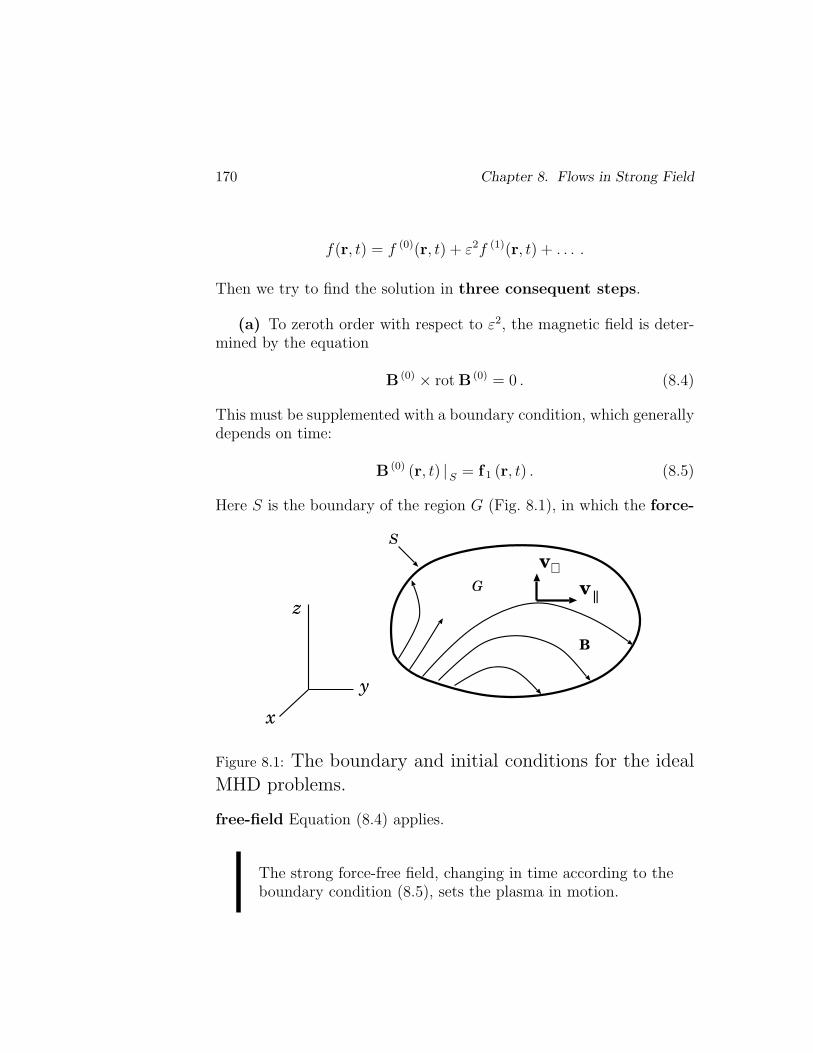
170 Chapter 8. Flows in Strong Field
f(r, t) = f (0)(r, t) + ε2f (1)(r, t) + . . . .
Then we try to find the solution in three consequent steps.
(a) To zeroth order with respect to ε2, the magnetic field is deter-mined by the equation
B (0) × rot B (0) = 0 . (8.4)
This must be supplemented with a boundary condition, which generallydepends on time:
B (0) (r, t) |S = f 1 (r, t) . (8.5)
Here S is the boundary of the region G (Fig. 8.1), in which the force-
x
zv
v
||
⊥
B
G
S
y
Figure 8.1: The boundary and initial conditions for the idealMHD problems.
free-field Equation (8.4) applies.
The strong force-free field, changing in time according to theboundary condition (8.5), sets the plasma in motion.
8.1. Formulation of Problem 171
(b) Kinematics of this motion is uniquely determined by two con-ditions.
The first one signifies the orthogonality of acceleration to the mag-netic field lines
B (0) · dv (0)
dt= 0 . (8.6)
This equation is the scalar product of Equation (8.1) and the vec-tor B(0).
The second condition is a consequence of the freezing-in Equa-tion (8.2)
∂ B (0)
∂t= rot
(v(0) ×B (0)
). (8.7)
Equations (8.6) and (8.7) determine the velocity v(0)(r, t), if the initialcondition inside the region G is given:
v(0)‖ (r, 0) |G = f 2 (r) . (8.8)
Here v(0)‖ is the velocity component along the field lines.
The velocity component across the field lines, v(0)⊥ , is uniquely de-
fined by the freezing-in Equation (8.7) at any moment, including theinitial one.
Therefore we do not need the initial condition for v(0)⊥ .
(c) Since we know the velocity field v(0)(r, t), the continuity equa-tion
∂ρ (0)
∂t+ div ρ (0)v(0) = 0 (8.9)
allows us to find the plasma density ρ (0)(r, t), if we know its initialdistribution
172 Chapter 8. Flows in Strong Field
ρ (0)(r, 0) |G = f3 (r) . (8.10)
Therefore,
at any moment of time,
the field B (0) (r, t) is found from Equation (8.4) and the boundarycondition (8.5).
Thereupon the velocity v(0)(r, t) is determined from Equations (8.6)and (8.7) and the initial condition (8.8).
Finally the continuity Equation (8.9) and the initial condition (8.10)give the plasma density ρ (0) (r, t).
We restrict our attention to the zeroth order relative to the pa-rameter ε2, neglecting the field deviation from a force-free state.
The question of the existence of solutions will be considered lateron, using 2D problems.
8.2 The formalism of 2D problems
Being relatively simple from the mathematical viewpoint, 2D idealMHD problems allow us to gain some general knowledge concerningthe actual flows of plasma with the frozen-in strong magnetic field.
The 2D problems are sometimes a close approximation of the real3D flows and can be used to compare the theory with experiments andobservations.
There are two types of problems treating the plane flows ofplasma, i.e. the flows with the velocity field
v = vx(x, y, t), vy(x, y, t), 0 .
All the quantities are dependent on variables x, y and t.
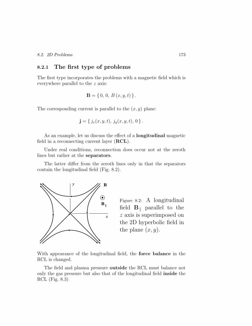
8.2. 2D Problems 173
8.2.1 The first type of problems
The first type incorporates the problems with a magnetic field which iseverywhere parallel to the z axis:
B = 0, 0, B (x, y, t) .
The corresponding current is parallel to the (x, y) plane:
j = jx(x, y, t), jy(x, y, t), 0 .
As an example, let us discuss the effect of a longitudinal magneticfield in a reconnecting current layer (RCL).
Under real conditions, reconnection does occur not at the zerothlines but rather at the separators.
The latter differ from the zeroth lines only in that the separatorscontain the longitudinal field (Fig. 8.2).
B
B ||
y
x
Figure 8.2: A longitudinalfield B ‖ parallel to thez axis is superimposed onthe 2D hyperbolic field inthe plane (x, y).
With appearance of the longitudinal field, the force balance in theRCL is changed.
The field and plasma pressure outside the RCL must balance notonly the gas pressure but also that of the longitudinal field inside theRCL (Fig. 8.3)
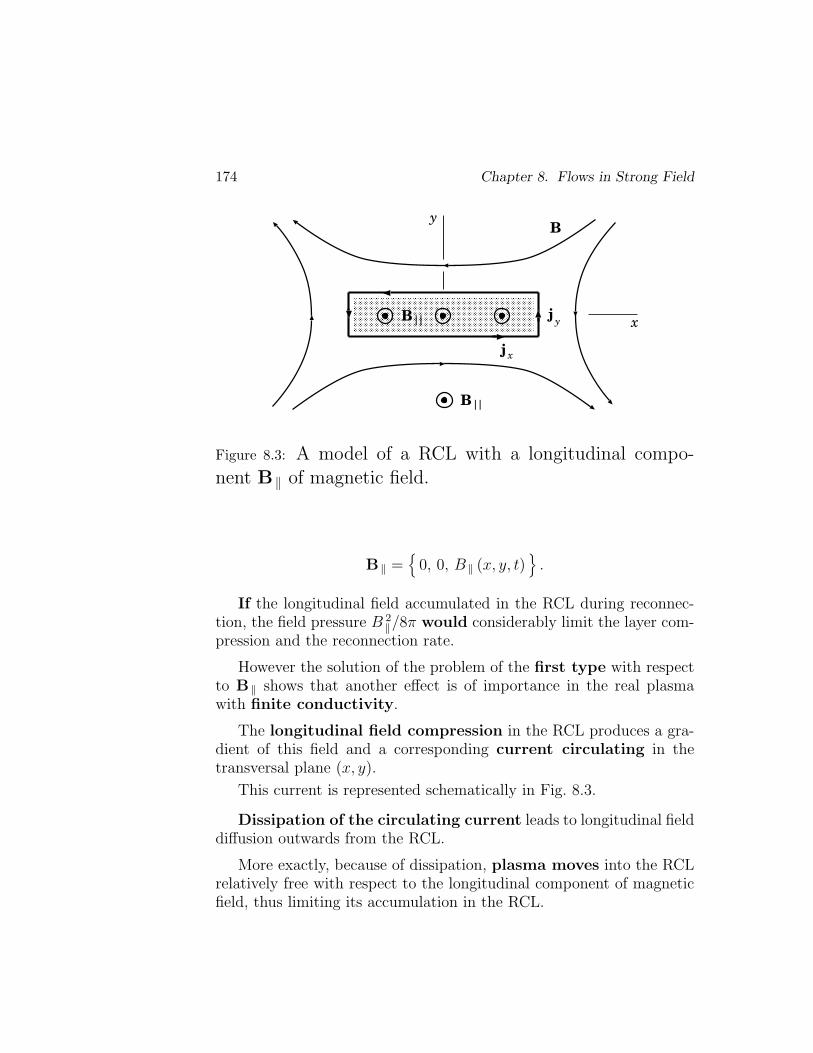
174 Chapter 8. Flows in Strong Field
B
j
jx
y x
y
B | |
B | |
Figure 8.3: A model of a RCL with a longitudinal compo-nent B ‖ of magnetic field.
B ‖ =
0, 0, B ‖ (x, y, t)
.
If the longitudinal field accumulated in the RCL during reconnec-tion, the field pressure B 2
‖/8π would considerably limit the layer com-pression and the reconnection rate.
However the solution of the problem of the first type with respectto B ‖ shows that another effect is of importance in the real plasmawith finite conductivity.
The longitudinal field compression in the RCL produces a gra-dient of this field and a corresponding current circulating in thetransversal plane (x, y).
This current is represented schematically in Fig. 8.3.
Dissipation of the circulating current leads to longitudinal fielddiffusion outwards from the RCL.
More exactly, because of dissipation, plasma moves into the RCLrelatively free with respect to the longitudinal component of magneticfield, thus limiting its accumulation in the RCL.
8.2. 2D Problems 175
8.2.2 The second type of MHD problems
8.2.2 (a) Magnetic field and its vector potential
The 2D problems of the second type treat the plane flows
v = vx(x, y, t), vy(x, y, t), 0 ,
associated with the plane magnetic field
B = Bx(x, y, t), By(x, y, t), 0 .
The currents corresponding to this field are parallel to the z axis
j = 0, 0, j (x, y, t) .
The vector-potential A has an its only non-zero component:
A = 0, 0, A (x, y, t) .
The magnetic field B is defined as
B =
∂A
∂y, − ∂A
∂x, 0
. (8.11)
The scalar function A (x, y, t) is often termed the vector potential.
This function is quite useful, owing to its properties.
Property 1.Substitute (8.11) in the differential equations describing the mag-
netic field lines
dx
Bx
=dy
By
=dz
Bz
.
These equations imply parallelism of the vector
d l = dx, dy, dz
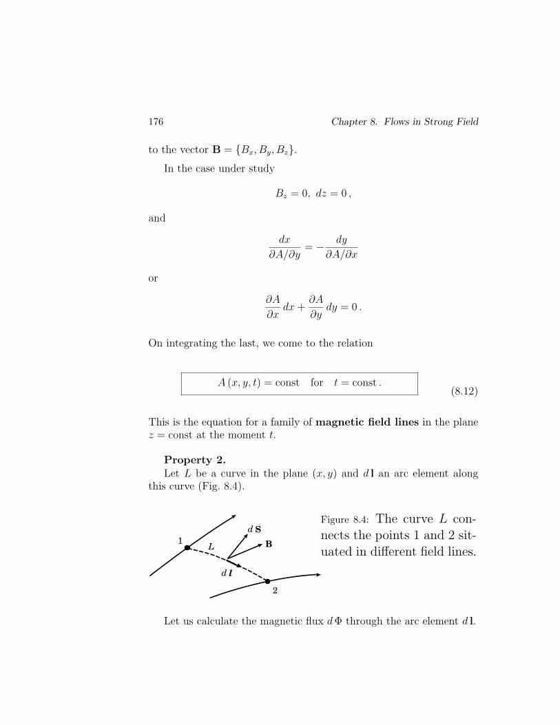
176 Chapter 8. Flows in Strong Field
to the vector B = Bx, By, Bz.In the case under study
Bz = 0, dz = 0 ,
and
dx
∂A/∂y= − dy
∂A/∂x
or
∂A
∂xdx +
∂A
∂ydy = 0 .
On integrating the last, we come to the relation
A (x, y, t) = const for t = const .(8.12)
This is the equation for a family of magnetic field lines in the planez = const at the moment t.
Property 2.Let L be a curve in the plane (x, y) and d l an arc element along
this curve (Fig. 8.4).
2
1 BL
d l
d S
Figure 8.4: The curve L con-nects the points 1 and 2 sit-uated in different field lines.
Let us calculate the magnetic flux d Φ through the arc element d l.
8.2. 2D Problems 177
By definition,
d Φ = B · dS = B · (ez × d l ) = B ·
∣∣∣∣∣∣∣∣∣∣∣
ex ey ez
0 0 1
dx dy 0
∣∣∣∣∣∣∣∣∣∣∣
=
= B · (−dy) ex + dx ey =
= −Bx dy + By dx . (8.13)
On substituting (8.11) in (8.13) we find
d Φ = −∂A
∂ydy − ∂A
∂xdx = − dA .
On integrating this along the curve L from point 1 to point 2 we obtainthe magnetic flux
Φ = A2 − A1 .
Thus the fixed value of the potential A is not only the field line ‘tag’determined by formula (8.12);
the difference of values of the vector potential A on two fieldlines is equal to the magnetic flux between them.
Simple rule:
Plot the field lines corresponding to equidistant values of A.
Property 3.
Let us substitute definition (8.11) in the freezing-in equation.
We obtain the following equation
rotdA
dt= 0 .
178 Chapter 8. Flows in Strong Field
Disregarding a gradient of an arbitrary function and considering thesecond type of 2D problems, we have
dA
dt≡ ∂A
∂t+ (v · ∇)A = 0 . (8.14)
This equation means that the lines
A (x, y, t) = const (8.15)
are Lagrangian lines: they move together with plasma.
According to (8.12) they are composed of the field lines.
Hence Equation (8.14) expresses the magnetic field freezing inplasma.
Thus we have one of the integrals of motion
A (x, y, t) = A (x0, y0, 0) ≡ A0(8.16)
at an arbitrary t.
Herex0, y0 are the coordinates of a “fluid particle” at the initial time
t = 0;x, y are the coordinates of the same particle at a moment of time t
or the coordinates of any other particle situated on the same fieldline A0 at the moment t.
Property 4.Equation of motion (8.1) rewritten in terms of the vector poten-
tial A(x, y, t) is of the form
ε2 dv
dt= −1
ρ∆A∇A . (8.17)
In the zeroth order relative to the small parameter ε2, outside thezeroth points (where∇A = 0) and the magnetic field sources (where∆A 6= 0) we have:
8.2. 2D Problems 179
∆A = 0 .(8.18)
So the vector potential is a harmonic function of variables x and y.
Hence, considering the (x, y) plane as a complex plane
z = x + i y ,
it is convenient to relate an analytic function F to the vector poten-tial A:
F (z, t) = A (x, y, t) + i A+(x, y, t) . (8.19)
Here A+(x, y, t) is a conjugate harmonic function connected withA (x, y, t) by the Cauchy-Riemann condition
A+(x, y, t) =∫ (
− ∂A
∂ydx +
∂A
∂xdy
)+ A+(t) =
= −∫
B · d l + A+(t) ,
where A+(t) is a quantity independent of the coordinates x and y.
The function F (z, t) is termed the complex potential.
The magnetic field vector
B = Bx + i By = − i
(dF
dz
)∗, (8.20)
the asterisk denoting the complex conjugation.
Now we can apply the methods of the complex variable functiontheory, in particular the method of conform mapping .
This has been done in order to determine the structure of mag-netic field:
180 Chapter 8. Flows in Strong Field
• in vicinity of reconnecting current layer (Syrovatskii, 1971),
• in solar coronal streamers (Somov and Syrovatskii, 1972)
• in the Earth’s magnetosphere (Oberz, 1973),
• the accretion disk magnetosphere (Somov et al., 2003).
Markovskii and Somov (1989) generalized the Syrovatskii model byattaching four shock MHD waves at the edges of the RCL.
The model reduces to the Riemann-Hilbert problem (in an analyticalform on the basis of the Christoffel-Schwarz integral) in order to analyzethe structure of magnetic field in vicinity of reconnection region (Bez-rodnykh et al., 2007).
8.2.2 (b) Motion of the plasma and its density
The motion kinematics due to changes in a potential field is uniquelydetermined by two conditions:
(i) the freezing-in condition and
(ii) the acceleration orthogonality with respect to the field lines
dv(0)
dt×∇A(0) = 0 . (8.21)
Equation (8.21) is a result of eliminating the unknown ∆A(1) from twocomponents of the vector equation
dv(0)
dt= − 1
ρ (0)∆A(1)∇A(0) . (8.22)
If x(t) and y(t) are the coordinates of a fluid particle, Equa-tions (8.21) and (8.14) are reduced to the ordinary differential equa-tions (Somov and Syrovatskii, 1976).
Once the kinematic part of the problem is solved, the trajectoriesof fluid particles are known:
8.3. Continuous MHD Flows 181
x = x (x0 , y0 , t) , y = y (x0 , y0 , t) . (8.23)
The fluid particle density change on moving along its trajectory is de-termined by the continuity Equation (8.3), rewritten in the Lagrangianform, and is equal to
ρ (x, y, t)
ρ0 (x0, y0)=
dU0
dU=D (x0, y0)
D (x, y). (8.24)
Here d U0 is the initial volume of a particle, dU is the volume of thesame particle at a moment of time t;
D (x0, y0)
D (x, y)=
∂x0
∂x
∂y0
∂y− ∂x0
∂y
∂y0
∂x(8.25)
is the Jacobian of the transformation that is inverse to the transforma-tion (8.23).
The 2D equations of the strong-field-cold-plasma approximation arerelatively simple but useful for applications to astrophysical plasmas.
In particular, they enable us to study the fast plasma flows in thesolar atmosphere and to understand some aspects of the reconnectionprocess.
In spite of their numerous applications, the list of exact so-lutions to them is rather poor. Still, we can enrich it signifi-cantly,
relying on many astrophysical objects, for example in the accretiondisk coronae and some mathematical ideas.
8.3 The existence of continuous flows
Thus, in the strong-field-cold-plasma approximation, the MHD equa-tions for a plane 2D flow of ideally conducting plasma (for the second-type problems) are reduced, in the zeroth order in the small parameterε2, to the following closed set of equations:
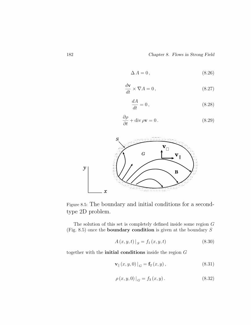
182 Chapter 8. Flows in Strong Field
∆ A = 0 , (8.26)
dv
dt×∇A = 0 , (8.27)
dA
dt= 0 , (8.28)
∂ρ
∂t+ div ρv = 0 . (8.29)
x
y
v
v
||
⊥
B
G
S
Figure 8.5: The boundary and initial conditions for a second-type 2D problem.
The solution of this set is completely defined inside some region G(Fig. 8.5) once the boundary condition is given at the boundary S
A (x, y, t) |S = f1 (x, y, t) (8.30)
together with the initial conditions inside the region G
v‖ (x, y, 0) |G = f2 (x, y) , (8.31)
ρ (x, y, 0) |G = f3 (x, y) . (8.32)
8.4. Time-dependent Magnetic Dipole 183
Here v ‖ is the velocity component along field lines.
Once the potential A (x, y, t) is known, the transversal velocity com-ponent is uniquely determined by the freezing-in Equation (8.28) andis equal, at any moment including the initial one, to
v⊥(x, y, t) = (v · ∇A)∇A
|∇A |2 = −∂A
∂t
∇A
|∇A |2 . (8.33)
The density ρ (x, y, t) is found from the continuity Equation (8.29)and the initial density distribution (8.32).
The next Section is devoted to an example which may have appli-cations.
8.4 Flows in a time-dependent dipole field
8.4.1 Plane magnetic dipole fields
Two parallel currents, equal in magnitude but opposite in direction, en-gender the magnetic field which far from the currents can be describedby a complex potential
F (z) =im
z, m = me iψ (8.34)
and is called the plane dipole field.
The quantity
m =2
cI l
has the meaning of the dipole moment,
I is the current magnitude,
l is the distance between the currents.
Formula (8.34) corresponds to the dipole situated at the origin ofcoordinates in the plane (x, y) and directed at an angle of ψ to thex axis.
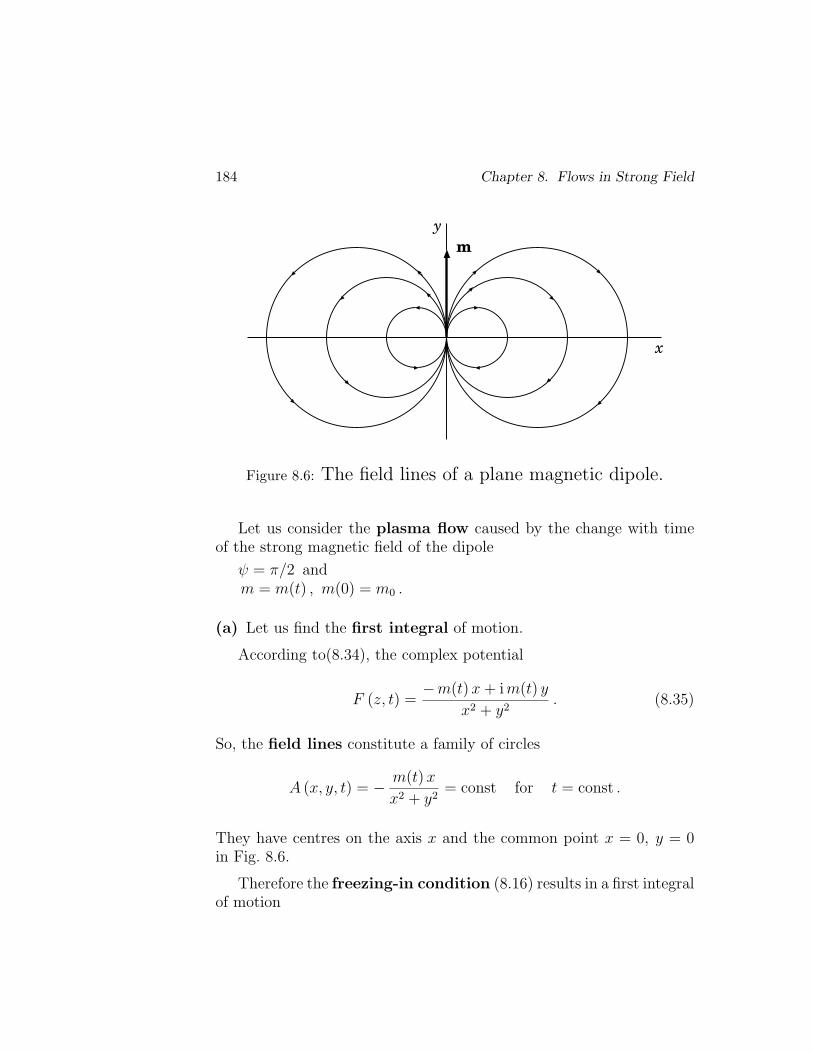
184 Chapter 8. Flows in Strong Field
m
x
y
Figure 8.6: The field lines of a plane magnetic dipole.
Let us consider the plasma flow caused by the change with timeof the strong magnetic field of the dipole
ψ = π/2 andm = m(t) , m(0) = m0 .
(a) Let us find the first integral of motion.
According to(8.34), the complex potential
F (z, t) =−m(t) x + i m(t) y
x2 + y2. (8.35)
So, the field lines constitute a family of circles
A (x, y, t) = − m(t) x
x2 + y2= const for t = const .
They have centres on the axis x and the common point x = 0, y = 0in Fig. 8.6.
Therefore the freezing-in condition (8.16) results in a first integralof motion
8.4. Time-dependent Magnetic Dipole 185
mx
x2 + y2=
m0 x0
x 20 + y 2
0
. (8.36)
Here x0, y0 are the coordinates of a fluid particle at the initial timet = 0 .
(b) The second integral is easily found in the limit of small changes ofthe dipole moment m (t) and respectively small plasma displacements.
Assuming the parameter
δ = vτ/L
to be small, Equation (7.26):
ε2 ∂v
∂t= − 1
ρB× rot B ,
which is linear in velocity.
The integration over time (with zero initial values for the velocity)allows us to reduce Equation (7.26) to the form
∂x
∂t= K(x, y, t)
∂A
∂x,
∂y
∂t= K(x, y, t)
∂A
∂y. (8.37)
Here K(x, y, t) is some function of coordinates and time.
Eliminating it from two Equations (8.37), we arrive at
∂y
∂x=
∂A
∂y
/∂A
∂x. (8.38)
Thus, not only the acceleration but also the plasma displacementsare normal to the field lines.
For dipole field, we obtain an ordinary differential equation
dy
dx=
2xy
x2 − y2.
Its integral
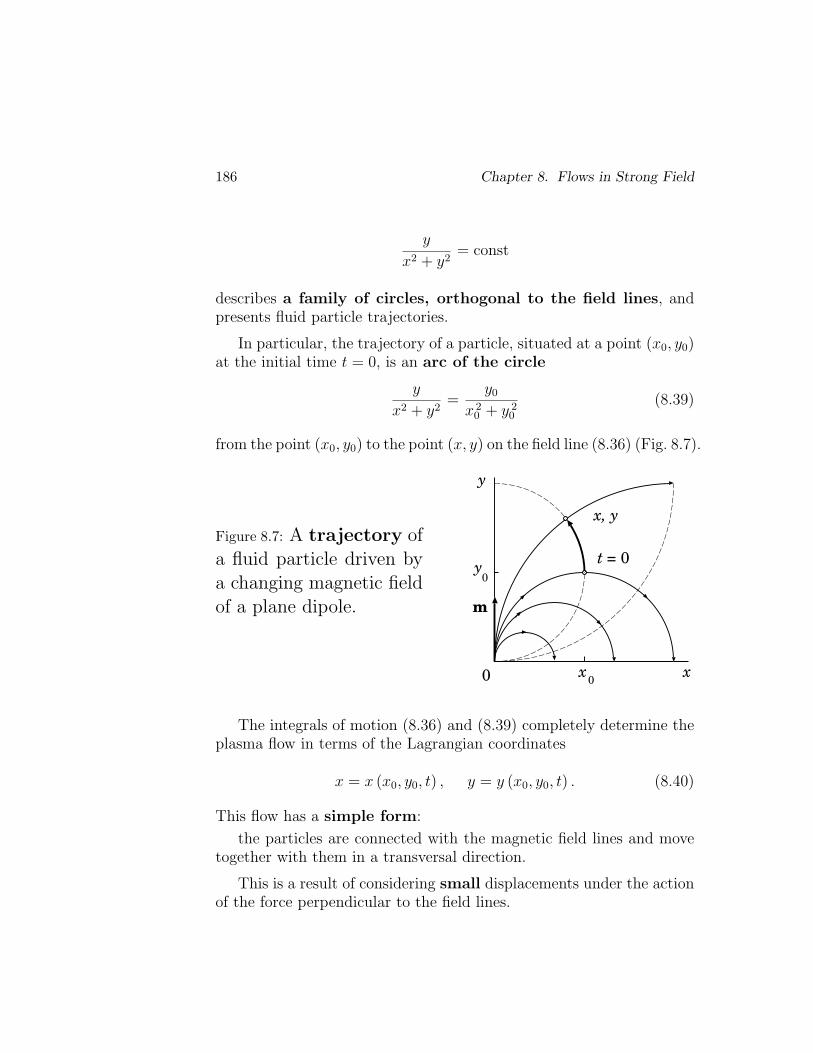
186 Chapter 8. Flows in Strong Field
y
x2 + y2= const
describes a family of circles, orthogonal to the field lines, andpresents fluid particle trajectories.
In particular, the trajectory of a particle, situated at a point (x0, y0)at the initial time t = 0, is an arc of the circle
y
x2 + y2=
y0
x 20 + y 2
0
(8.39)
from the point (x0, y0) to the point (x, y) on the field line (8.36) (Fig. 8.7).
Figure 8.7: A trajectory ofa fluid particle driven bya changing magnetic fieldof a plane dipole. m
x
y
y
yx,
x0
0
t = 0
0
The integrals of motion (8.36) and (8.39) completely determine theplasma flow in terms of the Lagrangian coordinates
x = x (x0, y0, t) , y = y (x0, y0, t) . (8.40)
This flow has a simple form:
the particles are connected with the magnetic field lines and movetogether with them in a transversal direction.
This is a result of considering small displacements under the actionof the force perpendicular to the field lines.
8.4. Time-dependent Magnetic Dipole 187
(c) The plasma density change.
On calculating the Jacobian for the transformation given by (8.36)and (8.39), we obtain the formula
ρ (x, y, t)
ρ0
=(
m
m0
)m 4
0
(m2x2 + m 20 y2)4
[m2x4 + m 2
0 y4+
+x2y2(3m2 −m 2
0
) ]2 −[2x2y2
(m 2
0 −m2)]2
. (8.41)
On the dipole axis (x = 0)
ρ (0, y, t)
ρ0
=m
m0
,
(8.42)
whereas in the ‘equatorial plane’ (y = 0)
ρ (x, 0, t)
ρ0
=(
m0
m
)3
. (8.43)
With increasing dipole moment m, the plasma density on thedipole axis grows proportionally to the moment,
whereas that at the equatorial plane falls in inverse proportion to thethird power of the moment.
The result pertains to the small changes in the dipole moment.
The exception is formula (8.42).
It applies to any changes of the dipole moment.
The acceleration of plasma is perpendicular to the field lines and iszero at the dipole axis.
Hence, if the plasma is motionless at the initial moment, arbitrarychanges of the dipole moment do not cause a plasma motion on thedipole axis (v = 0).
188 Chapter 8. Flows in Strong Field
Plasma displacements in the vicinity of the dipole axis always re-main small (δ ¿ 1) and the solution obtained applies.
(d) In the general case of arbitrarily large dipole moment changes,
the inertial effects resulting in plasma flows along the fieldlines are of considerable importance
(Somov and Syrovatskii, 1972).
The solution of the problem requires the integration of the ordi-nary differential equations that follows from Equation (8.21) andthe freezing-in Equation (8.14).
8.4.2 Axial-symmetric dipole fields
2D axial-symmetric problems can better suit the astrophysical applica-tions of the second-type problem considered.
The ideal MHD equations are written, using the approximation of astrong field and cold plasma, in spherical coordinates with due regardfor axial symmetry.
The role of the vector potential is fulfilled by the so-called streamfunction
Φ (r, θ, t) = r sin θ Aϕ(r, θ, t) . (8.44)
Here Aϕ is the only non-zero ϕ-component of the vector-potential A.
In terms of the stream functions, the equations take the form
dv
dt= ε−2K(r, θ, t)∇Φ ,
d Φ
dt= 0 ,
dρ
dt= −ρ div v ,
where
K(r, θ, t) =jϕ(r, θ, t)
ρ r sin θ(8.45)
(Somov and Syrovatskii, 1976).
8.4. Time-dependent Magnetic Dipole 189
The equations formally coincide with the corresponding Equations (8.17),(8.14) and (8.3) describing the plane flows in terms of the vector po-tential.
As a zeroth approximation in the small parameter ε2, we may take,for example, the dipole field.
In this case the stream function is of the form
Φ(0) (r, θ, t) = m(t)sin2 θ
r, (8.46)
where m(t) is a time-varying moment.
Let us imagine a magnetized ball of radius R(t) with the frozenfield B int(t).
The dipole moment of such a ball (a star or its envelope)
m(t) =1
2B int(t) R3(t) =
1
2π
(B0 πR 2
0
)R(t) . (8.47)
Here B0 and R0 are the values of B int(t) and R(t) at the initial timet = 0.
The second equality takes account of conservation of the flux
Bint(t) πR 2(t)
through the ball.
Formula (8.47) shows that the dipole moment of the ball is propor-tional to its radius R(t).
The solution to the problem (Somov and Syrovatskii, 1972a) showsthat as the dipole moment grows
the magnetic field rakes the plasma up to the dipole axis,compresses it and simultaneously accelerates it along thefield lines.
The density at the axis grows in proportion to the dipole moment,just as in the 2D plane case.
190 Chapter 8. Flows in Strong Field
∗ ∗ ∗
Envelopes of nova and supernova stars present a wide variety ofdifferent shapes.
It is common to find either flattened or stretched envelopes.
Their surface brightness is maximal at the ends of the main axes ofan oval image.
This can sometimes be interpreted as a gaseous ring observedalmost from an edge.
However, if there is no luminous belt between the brightness max-ima, then the remaining possibility is that single gaseous compressions– condensations – exist in the envelope.
At the early stages of the expansion, they give the impression thatthe nova ‘bifurcates’.
Suppose that the star’s magnetic field was a dipole one before theexplosion.
At the moment of the explosion a massive envelope with thefrozen-in field separated from the star and began to expand.
The expansion results in the growth of the dipole moment.
The field rakes the interstellar plasma surrounding the envelope,as well as external layers of the envelope, up in the direction of thedipole axis.
The process can be divided into two stages.
At the first one, the plasma is raked up by the field into the polarregions, a growth in density and pressure at the dipole axis taking place.
At the second stage, the increased pressure hinders the growth of thedensity, thus stopping compression, but the raking-up still continues.
The gas pressure gradient, arising ahead of the envelope, givesrise to the motion along the axis.
8.5. Practice 191
As a result, all the plasma is raked up into two compact conden-sates.
∗ ∗ ∗
If a magnetized ball compresses, plasma flows from the poles tothe equatorial plane, thus forming a dense disk or ring.
This is the old problem of astrophysics concerning the compressionof a gravitating cloud with a frozen-in field.
Magnetic raking-up of plasma into dense disks can work in the at-mospheres of collapsing stars.
8.5 Practice
Exercise 8.1. For a 3D field B, consider properties of the vector-potential A which is determined in terms of two scalar functions α andβ:
A = α∇β +∇ψ . (8.48)
Here ψ is an arbitrary scalar function.
Answer.
Formula (8.48) permits B to be written as
B = ∇α×∇β . (8.49)
HenceB · ∇α = 0 and B · ∇β = 0 . (8.50)
Thus ∇α and ∇β are perpendicular to the vector B, and functions αand β are constant along B.
The surfaces α = const and β = const are orthogonal to theirgradients and tangent to B.
Hence
192 Chapter 8. Flows in Strong Field
a magnetic field line can be conveniently defined in termsof a pair of values: α and β.
The functions α and β are referred to as Euler potentials or Clebschvariables.
Advantage of these variables appears in the study of field line mo-tions.
Exercise 8.2. Evaluate the typical value of the dipole moment for aneutron star.
Answer.
Typical neutron stars have B ∼ 1012 G.
With the star radius R ∼ 10 km, it follows from formula (8.47) that
m ∼ 1030 G cm3 .
Some of neutron stars are the spinning super-magnetized neutronstars created by supernova explosions.
The rotation of such stars called magnetars is slowing down sorapidly that a super-strong field,
B ∼ 1015 G ,
could provide so fast braking.
For a magnetarm ∼ 1033 G cm3 .
Exercise 8.3. Show that, prior to a solar flare, the magnetic energydensity in the corona is of about three orders of magnitude greater thanany of the other types.
Exercise 8.4. By using the method of conform mapping, deter-mine the shape of a magnetic cavity, magnetosphere, created by aplane dipole inside a perfectly conducting uniform plasma with a gaspressure p0.
Answer.
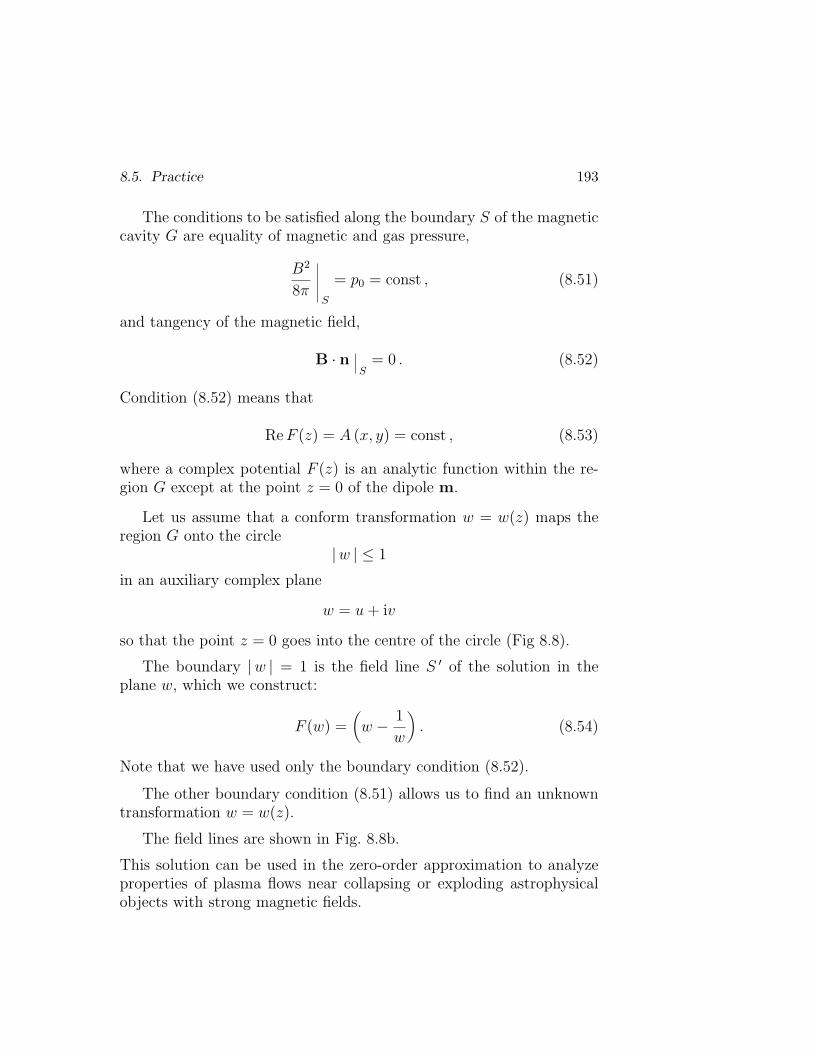
8.5. Practice 193
The conditions to be satisfied along the boundary S of the magneticcavity G are equality of magnetic and gas pressure,
B2
8πS
= p0 = const , (8.51)
and tangency of the magnetic field,
B · nS
= 0 . (8.52)
Condition (8.52) means that
Re F (z) = A (x, y) = const , (8.53)
where a complex potential F (z) is an analytic function within the re-gion G except at the point z = 0 of the dipole m.
Let us assume that a conform transformation w = w(z) maps theregion G onto the circle
|w | ≤ 1
in an auxiliary complex plane
w = u + iv
so that the point z = 0 goes into the centre of the circle (Fig 8.8).
The boundary |w | = 1 is the field line S ′ of the solution in theplane w, which we construct:
F (w) =(w − 1
w
). (8.54)
Note that we have used only the boundary condition (8.52).
The other boundary condition (8.51) allows us to find an unknowntransformation w = w(z).
The field lines are shown in Fig. 8.8b.
This solution can be used in the zero-order approximation to analyzeproperties of plasma flows near collapsing or exploding astrophysicalobjects with strong magnetic fields.
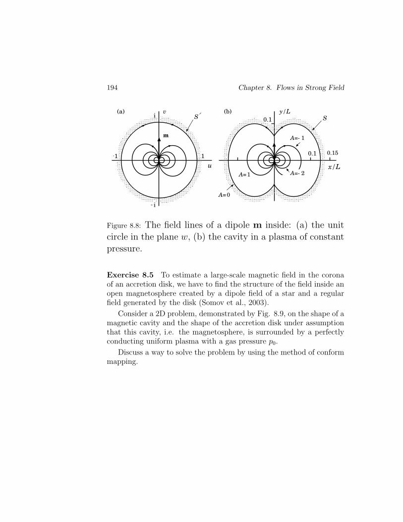
194 Chapter 8. Flows in Strong Field
u
vi S
10.15
x/L
y/L
0.1
A=
A=-
A=-A=
0
1
S
1
2
0.1
i
1
m
(a) (b)
Figure 8.8: The field lines of a dipole m inside: (a) the unitcircle in the plane w, (b) the cavity in a plasma of constantpressure.
Exercise 8.5 To estimate a large-scale magnetic field in the coronaof an accretion disk, we have to find the structure of the field inside anopen magnetosphere created by a dipole field of a star and a regularfield generated by the disk (Somov et al., 2003).
Consider a 2D problem, demonstrated by Fig. 8.9, on the shape of amagnetic cavity and the shape of the accretion disk under assumptionthat this cavity, i.e. the magnetosphere, is surrounded by a perfectlyconducting uniform plasma with a gas pressure p0.
Discuss a way to solve the problem by using the method of conformmapping.
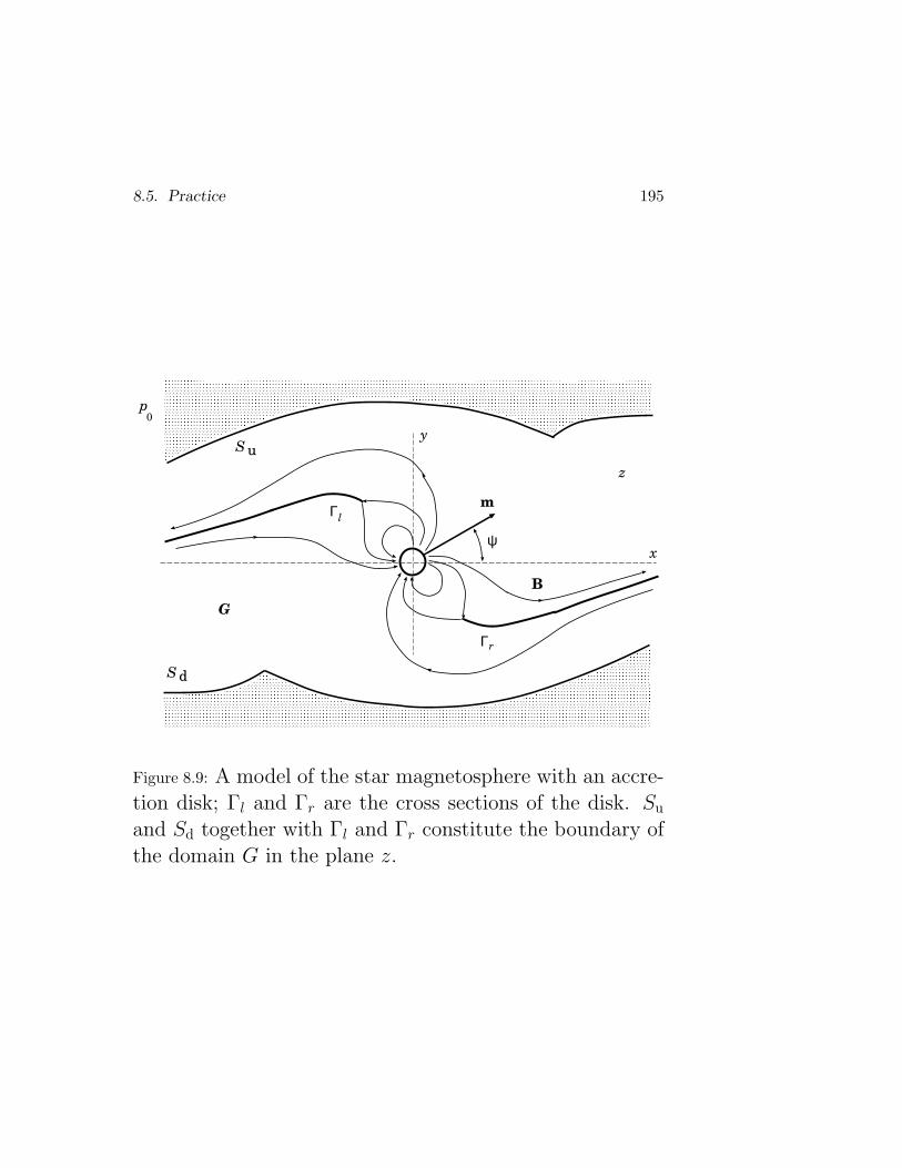
8.5. Practice 195
B
m
x
yS u
S d
ψ
Γ
Γ
z
G
l
r
p0
Figure 8.9: A model of the star magnetosphere with an accre-tion disk; Γl and Γr are the cross sections of the disk. Su
and Sd together with Γl and Γr constitute the boundary ofthe domain G in the plane z.


![Visual texts intro[1]](https://img.pdfslide.us/doc/110x75/546c1addaf7959680e8b570e/visual-texts-intro1.jpg)