Sun HPC ClusterTools™ 3.1 Performance Guide Alto, CA 94303-4900 USA 650 ... Administration Sun HPC ClusterTools 3.1 Administrator’s Guide 806-3731-10 ClusterTools Usage Sun HPC

Sun HPC ClusterTools™ 3.1

Performance Guide

ument to: [email protected] to: [email protected]

Part No. 806-3732-10March 2000, Revision A

Send comments about this docSend comments about this doc

Sun Microsystems, Inc.901 San Antonio RoadPalo Alto, CA 94303-4900 USA650 960-1300 Fax 650 969-9131

Copyright 2000 Sun Microsystems, Inc., 901 San Antonio Road, Palo Alto, California 94303-4900 U.S.A. All rights reserved.

This product or document is protected by copyright and distributed under licenses restricting its use, copying, distribution, and decompilation.

No part of this product or document may be reproduced in any form by any means without prior written authorization of Sun and its licensors,

if any. Third-party software, including font technology, is copyrighted and licensed from Sun suppliers.

Parts of the product may be derived from Berkeley BSD systems, licensed from the University of California. UNIX is a registered trademark in

the U.S. and other countries, exclusively licensed through X/Open Company, Ltd. For Netscape Communicator™, the following notice applies:

(c) Copyright 1995 Netscape Communications Corporation. All rights reserved.

Sun, Sun Microsystems, the Sun logo, SunStore, AnswerBook2, docs.sun.com, Solaris, Sun HPC ClusterTools, Prism, Sun Performance

WorkShop Fortran, Sun Performance Library, Sun WorkShop Compilers C, Sun WorkShop Compilers C++, Sun WorkShop Compilers Fortran,

Sun Visual WorkShop, and UltraSPARC are trademarks, registered trademarks, or service marks of Sun Microsystems, Inc. in the U.S. and other

countries. All SPARC trademarks are used under license and are trademarks or registered trademarks of SPARC International, Inc. in the U.S.

and other countries. Products bearing SPARC trademarks are based upon an architecture developed by Sun Microsystems, Inc.

The OPEN LOOK and Sun™ Graphical User Interface was developed by Sun Microsystems, Inc. for its users and licensees. Sun acknowledges

the pioneering efforts of Xerox in researching and developing the concept of visual or graphical user interfaces for the computer industry. Sun

holds a non-exclusive license from Xerox to the Xerox Graphical User Interface, which license also covers Sun’s licensees who implement OPEN

LOOK GUIs and otherwise comply with Sun’s written license agreements.

RESTRICTED RIGHTS: Use, duplication, or disclosure by the U.S. Government is subject to restrictions of FAR 52.227-14(g)(2)(6/87) and FAR

52.227-19(6/87), or DFAR 252.227-7015(b)(6/95) and DFAR 227.7202-3(a).

DOCUMENTATION IS PROVIDED “AS IS” AND ALL EXPRESS OR IMPLIED CONDITIONS, REPRESENTATIONS AND WARRANTIES,

INCLUDING ANY IMPLIED WARRANTY OF MERCHANTABILITY, FITNESS FOR A PARTICULAR PURPOSE OR NON-INFRINGEMENT,

ARE DISCLAIMED, EXCEPT TO THE EXTENT THAT SUCH DISCLAIMERS ARE HELD TO BE LEGALLY INVALID.

Copyright 2000 Sun Microsystems, Inc., 901 San Antonio Road, Palo Alto, Californie 94303-4900 U.S.A. Tous droits réservés.

Ce produit ou document est protégé par un copyright et distribué avec des licences qui en restreignent l’utilisation, la copie, la distribution, et la

décompilation. Aucune partie de ce produit ou document ne peut être reproduite sous aucune forme, par quelque moyen que ce soit, sans

l’autorisation préalable et écrite de Sun et de ses bailleurs de licence, s’il y en a. Le logiciel détenu par des tiers, et qui comprend la technologie

relative aux polices de caractères, est protégé par un copyright et licencié par des fournisseurs de Sun.

Des parties de ce produit pourront être dérivées des systèmes Berkeley BSD licenciés par l’Université de Californie. UNIX est une marque

déposée aux Etats-Unis et dans d’autres pays et licenciée exclusivement par X/Open Company, Ltd. La notice suivante est applicable à

Netscape Communicator™: (c) Copyright 1995 Netscape Communications Corporation. Tous droits réservés.

Sun, Sun Microsystems, le logo Sun, AnswerBook2, docs.sun.com, Solaris , Sun HPC ClusterTools, Prism, Sun Performance WorkShop Fortran,

Sun Performance Library, Sun WorkShop Compilers C, Sun WorkShop Compilers C++, Sun WorkShop Compilers Fortran, Sun Visual

WorkShop, et UltraSPARC sont des marques de fabrique ou des marques déposées, ou marques de service, de Sun Microsystems, Inc. aux Etats-

Unis et dans d’autres pays. Toutes les marques SPARC sont utilisées sous licence et sont des marques de fabrique ou des marques déposées de

SPARC International, Inc. aux Etats-Unis et dans d’autres pays. Les produits portant les marques SPARC sont basés sur une architecture

développée par Sun Microsystems, Inc.

L’interface d’utilisation graphique OPEN LOOK et Sun™ a été développée par Sun Microsystems, Inc. pour ses utilisateurs et licenciés. Sun

reconnaît les efforts de pionniers de Xerox pour la recherche et le développement du concept des interfaces d’utilisation visuelle ou graphique

pour l’industrie de l’informatique. Sun détient une licence non exclusive de Xerox sur l’interface d’utilisation graphique Xerox, cette licence

couvrant également les licenciés de Sun qui mettent en place l’interface d’utilisation graphique OPEN LOOK et qui en outre se conforment aux

licences écrites de Sun.

CETTE PUBLICATION EST FOURNIE "EN L’ETAT" ET AUCUNE GARANTIE, EXPRESSE OU IMPLICITE, N’EST ACCORDEE, Y COMPRIS

DES GARANTIES CONCERNANT LA VALEUR MARCHANDE, L’APTITUDE DE LA PUBLICATION A REPONDRE A UNE UTILISATION

PARTICULIERE, OU LE FAIT QU’ELLE NE SOIT PAS CONTREFAISANTE DE PRODUIT DE TIERS. CE DENI DE GARANTIE NE

S’APPLIQUERAIT PAS, DANS LA MESURE OU IL SERAIT TENU JURIDIQUEMENT NUL ET NON AVENU.

PleaseRecycle

Preface

The Sun HPC ClusterTools 3.1 Performance Guide presents techniques that application

programmers can use to get top performance from message-passing programs

running on Sun™ servers and clusters of servers.

Using Solaris Commands

This document may not contain information on basic Solaris™ commands and

procedures such as shutting down the system, booting the system, and configuring

devices.

See one or more of the following for this information:

■ AnswerBook2™ online documentation for the Solaris™ software environment

■ Other software documentation that you received with your system

iii

Typographic Conventions

Shell Prompts

Typeface orSymbol Meaning Examples

AaBbCc123 The names of commands, files,

and directories; on-screen

computer output

Edit your .login file.

Use ls -a to list all files.

% You have mail .

AaBbCc123 What you type, when

contrasted with on-screen

computer output

% suPassword:

AaBbCc123 Book titles, new words or terms,

words to be emphasized

Read Chapter 6 in the User’s Guide.

These are called class options.

You must be superuser to do this.

Command-line variable; replace

with a real name or value

To delete a file, type rm filename.

Shell Prompt

C shell machine_name%

C shell superuser machine_name#

Bourne shell and Korn shell $

Bourne shell and Korn shell superuser #

iv Sun HPC ClusterTools 3.1 Performance Guide • March 2000

Related Sun Documentation

Ordering Sun Documentation

Fatbrain.com, an Internet professional bookstore, stocks select product

documentation from Sun Microsystems, Inc.

For a list of documents and how to order them, visit the Sun Documentation Center

on Fatrain.com at:

http://www1.fatbrain.com/documentation/sun

Application Title Part Number

All Read Me First: Guide to Sun HPCClusterTools Documentation

806-3729-10

All Sun HPC ClusterTools 3.1 Product Notes 806-4182-10

Installation Sun HPC ClusterTools 3.1 InstallationGuide

806-3730-10

SCI Sun HPC SCI 3.1 Guide 806-4183-10

Administration Sun HPC ClusterTools 3.1 Administrator’sGuide

806-3731-10

ClusterTools Usage Sun HPC ClusterTools 3.1 User’s Guide 806-3733-10

Sun MPI Programming Sun MPI 4.1 Programming and ReferenceGuide

806-3734-10

Sun S3L Programming Sun S3L 3.1 Programming and ReferenceGuide

806-3735-10

Prism Environment Prism 6.1 User’s Guid 806-3736-10

Prism Environment Prism 6.1 Reference Manual 806-3737-10

v

Accessing Sun Documentation Online

The docs.sun.com SM web site enables you to access Sun technical documentation

on the Web. You can browse the docs.sun.com archive or search for a specific book

title or subject at:

http://docs.sun.com

Sun Welcomes Your Comments

We are interested in improving our documentation and welcome your comments

and suggestions. You can email your comments to us at:

[email protected]

Please include the part number (806-3732-10) of your document in the subject line of

your email.

vi Sun HPC ClusterTools 3.1 Performance Guide • March 2000

CHAPTER 1

Introduction: The Sun HPCClusterTools Solution

The Sun HPC ClusterTools suite is a solution for high-performance computing. It

provides the tools you need to develop and execute parallel (message-passing)

applications. These programs can run on any Sun UltraSPARC™-based system, from

a single workstation up to a cluster of high-end symmetric multiprocessors (SMPs).

Computing power on this scale has traditionally been used for scientific problems

and simulations. More recently, there has been an explosive growth in the

application of HPC to business problems, such as decision support, data rollups,

financial analysis, data mining, and bioinformatics.

This chapter briefly describes the components of the Sun HPC ClusterTools solution

and notes how each contributes to the goal of high performance.

The remainder of this manual presents the techniques by which ClusterTools users

can get the best performance from their applications.

■ Chapter 2 - Choosing Your Programming Model and Hardware■ Chapter 3 - Performance Programming with the Sun MPI (message-passing) library

■ Chapter 4 - Sun S3L Performance Guidelines, for getting the most from this

optimized library of scientific routines

■ Chapter 5 - Compilation and Linking for top performance

■ Chapter 6 - Runtime Considerations and Tuning■ Appendix A - A quick Summary of Performance Tips■ Appendix B - Sun MPI Implementation and how it affects performance

■ Appendix C - Sun MPI Environment Variables and how to use them

1

Sun HPC HardwarePrograms written with Sun HPC ClusterTools software are binary-compatible across

the whole line of Sun UltraSPARC servers and workstations. This feature allows

users to exploit all available hardware in achieving performance.

For top performance, you can choose the large Sun Enterprise SMPs. These range

from a 4-processor workgroup server up to the 64-processor Enterprise™ 10000 (the

Starfire™). For even more demanding applications, multiple SMPs can be configured

into a cluster using a variety of Sun-supported interconnects.

This section notes the performance-related features of Sun SMPs and clusters. These

will be important in the first step of performance programming, choosing your tools

and hardware, discussed in Chapter 2.

Processors

The heart of a Sun HPC system is the UltraSPARC processor. A Sun SMP may

contain up to 64 such processors.

The latest generation is the UltraSPARC II, a superscalar 64-bit RISC processor. A

single UltraSPARC II running at 400 MHz provides dual launch floating-point

capability that results in a peak performance of 800 Mflops.

Nodes

Each SMP is a multiprocessor, shared-memory server. Although an SMP may be a

node of a cluster, each SMP scales sufficiently to support a large proportion of HPC

applications itself. By permitting an application to run within a single node, the SMP

offers the simplest and fastest programming and operations environment. Given

shared, symmetrical access to the node’s memory, users need not manage data

location or interprocessor data transfers for a single-node parallel application.

The nodes may have one of several processor-to-memory interconnects, depending

on the number of CPUs in the node. These range from a simple 1.6 GB/s processor-

to-memory interconnect, used in nodes of up to 4 processors, up to the Gigaplane-

XB, which combines a 16x16 data crossbar switch with 4-way parallel point-to-point

address routers to achieve up to 12.5 GB/s and support up to 64 processors. This

progression of interconnect technology permits high-speed memory access

regardless of node size.

2 Sun HPC ClusterTools 3.1 Performance Guide • March 2000

Clusters

For even more compute-intensive applications, SMPs may be configured into a

cluster of any size. Each unit of shared memory (i.e., each SMP) serves as a node of

the cluster, and the programmer must manage the location of data in the distributed

memory and its transfers between nodes.

Individual Sun HPC ClusterTools message-passing applications can have up to 1024

processes running on as many as 64 nodes of a cluster.

Interconnects

The recommended low-latency interconnect technology for clustering Sun HPC

servers is the Scalable Coherent Interface (SCI), which can connect up to 4 nodes.

Remote Shared Memory (RSM) software supports SCI.

Larger clusters can be built using any Sun-supported TCP/IP interconnect, such as

100BaseT Ethernet or ATM.

Sun HPC ClusterTools SoftwareSun’s HPC message-passing software supports applications designed to run on

single systems and clusters of SMPs. Called Sun HPC ClusterTools software, it

provides the tools for developing distributed-memory parallel applications and for

managing distributed resources in the execution of these applications.

Sun HPC ClusterTools 3.1 software runs under the Solaris 2.6, Solaris 7, and Solaris

8 (32-bit or 64-bit) operating environments.

Another software suite, Sun WorkShop™ software, can be used to develop shared-

memory applications. These may be multithreaded or may be parallelized to some

extent during compilation, but they are limited to running within a single SMP.

Programmers can use tools from both the Sun WorkShop suite and the HPC

ClusterTools suite to develop distributed-memory applications that also exhibit

parallelism (multithreading) within nodes.

The differences between HPC ClusterTools software and Sun WorkShop software are

explored in Chapter 2. The present chapter focuses on describing the capabilities of

Sun HPC ClusterTools 3.1 software.

The ClusterTools suite is layered on the Sun WorkShop suite, and uses its compilers

for C, C++, Fortran 77, and Fortran 90. However, the ClusterTools suite provides

specialized versions of development tools for its message-passing programs:

Chapter 1 Introduction: The Sun HPC ClusterTools Solution 3

■ Sun MPI library of message-passing and I/O routines

■ Sun S3L, an optimized scientific subroutine library

■ Sun Parallel File System, for use with MPI I/O

■ Prism™ graphical development environment for debugging and performance

profiling of message-passing programs

■ Sun CRE, a runtime environment that manages the resources of a server or cluster

to execute message-passing programs

■ Sun runtime environment plugins for use with Platform Computing’s LSF

resource management suite (an alternative to the CRE)

Sun MPI

Sun MPI is a highly optimized version of the Message-Passing Interface (MPI)

communications library. This dynamic library is the basis of distributed-memory

programming, as it allows the programmer to create distributed data structures and

to manage interprocess communications explicitly.

MPI is the de facto industry standard for message-passing programming. You can

find more information about it on the World Wide Web at the MPI home page and

the many links it provides:

http://www.mpi-forum.org

Sun MPI implements all of the MPI 1.2 standard as well as a significant subset of the

MPI 2.0 feature list. In addition, Sun MPI provides the following features:

■ Seamless use of different network protocols; for example, code compiled on a Sun

HPC system that has a Scalable Coherent Interface (SCI) network can be run

without change on a cluster that has an ATM network.

■ Multiprotocol, thread-safe support such that MPI picks the fastest available

medium for each type of connection (such as shared memory, SCI, or ATM).

■ Finely tunable shared-memory communication.

■ Optimized collectives for SMPs, for long messages, for clusters, etc.

■ Parallel I/O to the ClusterTools Parallel (distributed) File System, as well as

single-stream I/O to a standard Solaris file system (UFS).

Sun MPI programs are compiled on Sun WorkShop compilers. MPI provides full

support for Fortran 77, C, and C++, and basic support for Fortran 90.

Chapter 3 and Appendix B of this manual provide more information about Sun

MPI’s features, as well as instructions for getting the best performance from an MPI

program.


Sun S3L

The Sun Scalable Scientific Subroutine Library (Sun S3L) provides a set of parallel

and scalable capabilities and tools that are used widely in scientific and engineering

computing. Built on top of MPI, it provides highly optimized implementations of

vector and dense matrix operations (level 1, 2, 3 Parallel BLAS), FFT, tridiagonal

solvers, sorts, matrix transpose, and many other operations. Sun S3L also provides

optimized versions of a subset of the ScaLAPACK library, along with utility routines

to convert between S3L and ScaLAPACK descriptors.

S3L is thread-safe and also supports the multiple instance paradigm, which allows

an operation to be applied concurrently to multiple, disjoint data sets in a single call.

Sun S3L routines can be called from applications written in F77, F90, C, and C++.

This library is described in more detail in Chapter 4.

Sun Parallel File System

Sun HPC ClusterTools’s Parallel File System (PFS) component provides high-

performance file I/O for MPI applications running in a cluster-based, distributed-

memory environment.

PFS files closely resemble UFS files, but they provide significantly higher file I/O

performance by striping files across multiple nodes. This means that the time

required to read or write a PFS file can be reduced by an amount roughly

proportional to the number of file server nodes in the PFS file.

Sun PFS is optimized for the large files and complex data access patterns that are

characteristic of HPC applications.

Prism Environment

The Prism environment is the Sun HPC ClusterTools graphical programming

environment. It allows you to develop, execute, and debug multithreaded or

unthreaded message-passing programs and to visualize data at any stage in the

execution of a program.

The Prism environment also supports performance profiling of message-passing

programs. The analysis provides an overview of what MPI calls, message sizes, or

other characteristics account for the execution time. You can display information

about the sort of message-passing activity in different phases of a run, identify "hot

spot" events, and, with simple mouse clicks, investigate any of them in detail.

The Prism profiling capabilities are described in more detail in Chapter 7. It can be

used with applications written in Fortran 77, Fortran 90, C, and C++.

Chapter 1 Introduction: The Sun HPC ClusterTools Solution 5

Cluster Runtime Environment

The Cluster Runtime Environment (CRE) component of Sun HPC ClusterTools

software serves as the runtime resource manager for message-passing programs. It

supports interactive execution of Sun HPC applications on single SMPs or on

clusters of SMPs.

CRE is layered on the Solaris operating environment but enhanced to support

multiprocess execution. It provides the tools for configuring and managing clusters,

nodes, logical sets of processors (partitions), and PFS I/O servers.

Alternatively, Sun HPC message-passing programs can be executed by third-party

resource-management software, such as the Load Sharing Facility™ suite from

Platform Computing.


CHAPTER 2

Choosing Your Programming Modeland Hardware

The first step in developing a high-performance application is to settle upon your

basic approach. To make the best choice among the Sun HPC tools and techniques,

you need to:

■ Set goals for program performance and scalability

■ Determine the amount of time and effort you can invest

■ Select a programming model

■ Assess the available computing resources

There are two common models of parallel programming in high performance

computing: shared-memory programming and distributed-memory programming.

These models are supported on Sun hardware with Sun WorkShop software and

with Sun HPC ClusterTools software, respectively. Issues in choosing between the

models may include existing source-code base, available software development

resources, desired scalability, and target hardware.

As detailed in Chapter 1, the basic Sun HPC ClusterTools programming model is

distributed-memory message passing. Such a program executes as a collection of

Solaris processes with separate address spaces. The processes compute

independently, each on its own local data, and share data only through explicit calls

to message-passing routines.

You may choose to use this model regardless of your target hardware. That is, you

might run a message-passing program on an SMP cluster or run it entirely on a

single, large SMP server. Or, you may choose to forego ClusterTools software and

utilize only multithreaded parallelism, running in on a single SMP server. It is also

possible to combine the two approaches.

This chapter provides a high-level overview of how to assess programming models

on Sun parallel hardware.

7

Programming ModelA high-performance application will almost certainly be parallel, but parallelism

comes in many forms. The form you choose depends partly on your target hardware

(server versus cluster) and partly on the time you have to invest.

Sun provides development tools for several widely used HPC programming models.

These products are categorized by memory model: Sun WorkShop tools for shared-

memory programming and Sun HPC ClusterTools for distributed-memory

programming.

■ Shared memory means that all parts of a programs can access one another’s data

freely. This may be because they share a common address space, which is the case

with multiple threads of control within a single process. Or, it may result from

employing a mechanism for sharing memory (one such is mmap).

Parallelism that is generated by Sun WorkShop compilers or programmed as

multiple threads requires either a single processor or an SMP. SMP servers give

their executing processes equal (“symmetric”) access to their shared memory.

■ Distributed memory means that multiple processes exchange data only through

explicit message-passing.

Message-passing programs, where the programmer inserts calls to the MPI

library, are the only programs that can run across a cluster of SMPs. They can

also, of course, run on a single SMP or even on a serial processor.

Table 2.1 summarizes these two product suites.

TABLE 2-1 Comparison of Sun WorkShop and Sun HPC ClusterTools Suites

Sun WorkShop Suite Sun HPC ClusterTools Suite

Target hardware Any Sun workstation or

SMP

Any Sun workstation, SMP,

or cluster

Memory model Shared memory Distributed memory

Runtime resource manager Solaris operating

environment

CRE (Cluster Runtime

Environment) or third-party

suite

Parallel execution Multithreaded Multiprocess with message

passing


Thus, available hardware does not necessarily dictate programming model. A

message-passing program can run on any configuration, and a multithreaded

program can run on a parallel server (SMP). The only constraint is that a program

without message-passing cannot run on a cluster.

The choice of programming model, therefore, usually depends more on software

preferences and available development time. Only when your performance goals

demand the combined resources of a cluster of servers is the message-passing model

necessarily required.

A closer look at the differences between shared-memory model and the distributed

memory model as they pertain to parallelism reveals some other factors in the

choice. The differences are summarized in Table 2.2.

Note – Nonuniform memory architecture (NUMA) is starting to blur the lines

between shared and distributed memory architectures. That is, the architecture

functions as shared memory, but typically the differences in cost between local and

remote memory accesses is so great that it may be desirable to manage data locality

explicitly. One way to do this is to use message passing.

Even without a detailed look, it is obvious that more parallelism is available with

less investment of effort in the shared memory-model.

To illustrate the difference, consider a simple program that adds the values of an

array (a global sum). In serial Fortran, the code is:

TABLE 2-2 Comparison of Shared-Memory and Distributed-Memory Parallelism

Shared Memory Distributed Memory

Parallelization unit Loop Data structure

Compiler-generatedparallelism

Available in Fortran 77,

Fortran 90, and C via

compiler options, directives/

pragmas, and OpenMP

HPF (not part of

ClusterTools suite)

Explicit (hand-coded)parallelism

C/C++ and threads (Solaris

or POSIX)

Calls to MPI library routines

from Fortran 77, Fortran 90,

C, or C++

REAL A(N), X X = 0. DO I = 1, N X = X + A(I) END DO

Chapter 2 Choosing Your Programming Model and Hardware 9

Compiler-generated parallelism requires little change. In fact, the compiler may well

parallelize this simple example automatically. At most, the programmer may need to

add a single directive:

To perform this operation with an MPI program, the programmer needs to

parallelize the data structure as well as the computational loop. The program would

look like this:

When this program executes, each process can access only its own (local) share of the

data array. Explicit message passing is used to combine the results of the multiple

concurrent processes.

Clearly, message passing requires more programming effort than shared-memory

parallel programming. But this is only one of several factors to consider in choosing

a programming model. The trade-off for the increased effort can be a significant

increase in performance and scalability.

In choosing your programming model, consider the following factors:

■ If you are updating an existing code, what programming model does it use? In

some cases, it is reasonable to migrate from one model to another, but this is

rarely easy. For example, to go from shared memory to distributed memory, you

must parallelize the data structures and redistribute them throughout the entire

source code.

■ What time investment are you willing to make? Compiler-based multithreading

(using Sun WorkShop tools) may allow you to port or develop a program in less

time than explicit message passing would require.

REAL A(N), X X = 0. C$PAR DOALL, REDUCTION DO I = 1, N X = X + A(I) END DO

REAL A(NLOCAL), X, XTMP

XTMP = 0. DO I = 1, NLOCAL XTMP = XTMP + A(I) END DO CALL MPI_ALLREDUCE & (XTMP,X1,MPI_REAL,MPI_SUM,MPI_COMM_WORLD,IERR)


■ What is your performance requirement? Is it within or beyond the computing

capability associated with a single, uniform memory? Since Sun SMP servers can

be very large—up to 64 processors in the current generation—a single server (and

thus shared memory) may be adequate for some purposes. For other purposes, a

cluster—and thus distributed-memory programming—will be required.

■ Is your performance requirement (including problem size) likely to increase in the

future? If so, it may be worth choosing the message-passing model even if a

single server meets your current needs. You can then migrate easily to a cluster in

the future. In the meantime, the application may run faster than a shared-memory

program on a single SMP because of the MPI discipline of enforcing data locality.

Mixing models is generally possible, but not common.

ScalabilityA part of setting your performance goals is to consider how your application will

scale.

The primary purpose of message-passing programming is to introduce explicit data

decomposition and communication into an application, so that it will scale to higher

levels of performance with increased resources. The appeal of a cluster is that it

increases the range of scalability: a potentially limitless amount of processing power

may be applied to complex problems and huge data sets.

The degree of scalability you can realistically expect is a function of the algorithm,

the target hardware, and certain laws of scaling itself.

Amdahl’s Law

First, the bad news. Decomposing a problem among more and more processors

ultimately reaches a point of diminishing returns. This idea is expressed in a formula

known as Amdahl’s Law.1 Amdahl’s Law assumes (quite reasonably) that a task has

only some fraction f that is parallelizable, while the rest of the task is inherently

serial. As the number of processors NP is increased, the execution time T for the task

decreases as

T = (1-f) + f / NP

1. G.M. Amdahl, Validity of the single-processor approach to achieving large scale computing capabilities. InAFIPS Conference Proceedings, vol. 30 (Atlantic City, N.J., Apr. 18-20). AFIPS Press, Reston, Va., 1967, pp. 483-485.


For example, consider the case in which 90 percent of the workload can be

parallelized. That is, f = 0.90 . The speedup as a function of the number of

processors is shown in Table 2-3.

As the parallelizable part of the task is more and more subdivided, the non-parallel

10 percent of the program (in this example) begins to dominate. The maximum

speedup achievable is only 10-fold, and the program can actually use only about

three or four processors efficiently.

Keep Amdahl’s Law in mind when you target a performance level or run prototypes

on smaller sets of CPUs than your production target. In the example above, if you

had started measuring scalability on only two processors, the 1.8-fold speedup

would have seemed admirable, but it is actually an indication that scalability beyond

that may be quite limited.

In another respect, the scalability story is even worse than Amdahl’s Law suggests.

As the number of processors increases, so does the overhead of parallelization. Such

overhead may include communication costs or interprocessor synchronization. So,

observation will typically show that adding more processors will ultimately cause

not just diminishing returns but negative returns: eventually, execution time may

increase with added resources.

Still, the news is not all bad. With the high-speed interconnects within and between

nodes, as described in Chapter 1, and with the programming techniques described in

this manual, your application may well achieve high, and perhaps near linear,

TABLE 2-3 Speedup with Number of Processors

Processors(NP)

Run time(T)

Speedup(1/T) Efficiency

1 1.000 1.0 100%

2 0.550 1.8 91%

3 0.400 2.5 83%

4 0.325 3.1 77%

6 0.250 4.0 67%

8 0.213 4.7 59%

16 0.156 6.4 40%

32 0.128 7.8 24%

64 0.114 8.8 14%


speedups for some number of processors. And, in certain situations, you may even

achieve superlinear scalability, since adding processors to a problem also provides a

greater aggregate cache.

Scaling Laws of Algorithms

Amdahl’s Law assumes that the work done by a program is either serial or

parallelizable. In fact, an important factor for distributed-memory programming that

Amdahl’s Law neglects is communication costs. Communication costs increase as

the problem size increases, although their overall impact depends on how this term

scales vis-a-vis the computational workload.

When the local portion (the subgrid) of a decomposed data set is sufficiently large,

local computation can dominate the run time and amortize the cost of interprocess

communication. Table 2-4 shows examples of how computation and communication

scale for various algorithms. In the table, L is the linear extent of a subgrid while Nis the linear extent of the global array.

With a sufficiently large subgrid, the relative cost of communication can be lowered

for most algorithms.

The actual speed-up curve depends also on cluster interconnect speed. If a problem

involves many interprocess data transfers over a relatively slow network

interconnect, the increased communication costs of a high process count may exceed

the performance benefits of parallelization. In such cases, performance may be better

with fewer processes collocated on a single SMP. With a faster interconnect, on the

other hand, you might see even superlinear scalability with increased process counts

because of the larger cache sizes available.

TABLE 2-4 Scaling of Computation and Communication Times for Selected Algorithms

Algorithm Communication TypeCommunicationCount

ComputationCount

2-dimensional stencil nearest neighbor L L2

3-dimensional stencil nearest neighbor L2 L3

matrix multiply nearest neighbor N2 N3

multidimensional

FFT

all-to-all N N log(N)


Characterizing PlatformsTo set reasonable performance goals, and perhaps to choose among available sets of

computing resources, you need to be able to assess the performance characteristics

of hardware platforms.

The most basic picture of message-passing performance is built on two parameters:

latency and bandwidth. These parameters are commonly cited for point-to-point

message passing, that is, simple sends and receives.

■ Latency is the time required to send a null-length message.

■ Bandwidth is the rate at which very long messages are sent.

In this somewhat simplified model, the time required for passing a message between

two processes is

time = latency + message-size / bandwidth

Obviously, short messages are latency-bound and long messages are bandwidth-

bound. The crossover message size between the two is given as

crossover-size = latency x bandwidth

Another performance parameter is bisection bandwidth, which is a measure of the

aggregate bandwidth a system can deliver to communication-intensive applications

that exhibit little data locality. Bisection bandwidth may not be related to point-to-

point bandwidth since the performance of the system can degrade under load (many

active processes).

To suggest orders of magnitude, Table 2.5 shows sample values of these parameters

for the current generation of Sun HPC platforms:

TABLE 2-5 Sample Performance Values for MPI Operations on Various Platforms

PlatformLatency(microseconds)

Bandwidth(Mbyte/s)

Crossover size= lat x bw(bytes)

PlatformBisectionbandwidth(Mbyte/s)

SMP E 10000 server ~ 2 ~ 200 ~ 400 ~ 2500

cluster:

4 nodes connected

with SCI and RSM

~ 10 ~ 50 ~ 500 ~ 200

cluster:

64 nodes connected

with TCP network

~ 150 ~ 40 ~ 6000 ~ 2000


Note that the best performance is likely to come from a single server. With Sun

servers, this means up to 64 CPUs in the current generation.

For clusters, these values indicate that the TCP cluster is much more latency-bound

than the smaller cluster using a faster interconnect. On the other hand, many nodes

are needed to match the bisection bandwidth of single node.

Basic Hardware Factors

Typically, you work with a fixed set of hardware factors: your system is what it is.

From time to time, however, hardware choices may be available, and, in any case,

you need to understand the ways in which your system affects program

performance. This section describes a number of basic hardware factors.

Processor speed is directly related to the peak floating-point performance a processor

can attain. Since an UltraSPARC processor can execute up to one floating-point

addition and one floating-point multiply per cycle, peak floating-point performance

is twice the processor clock speed. For example, a 250-MHz processor would have a

peak floating-point performance of 500 Mflops. In practice, achieved floating-point

performance will be less, due to imbalances of additions and multiplies and the

necessity of retrieving data from memory rather than cache. Nevertheless, some

number of floating-point intensive operations, such as the matrix multiplies that

provide the foundation for much of dense linear algebra, can achieve a high fraction

of peak performance, and typically increasing processor speed has a positive impact

on most performance metrics.

Large L2 (or external) caches can also be important for good performance. While it is

desirable to keep data accesses confined to L1 (or on-chip) caches, UltraSPARC

processors run quite efficiently from L2 caches as well. When you go beyond L2

cache to memory, however, the drop in performance can be significant. Indeed,

though Amdahl’s Law and other considerations suggest that performance should

scale at best linearly with processor counts, many applications see a range of

superlinear scaling, since an increase in processor count implies an increase in

aggregate L2 cache size.

The number of processors is, of course, a basic factor in performance since more

processors deliver potentially more performance. Naturally, it is not always possible

to utilize many processors efficiently, but it is vital that "enough" processors be

present. This means not only that there should be one processor per MPI process,

but ideally there should also be a few extra processors per node to handle system

daemons and other services.

System speed is a round fraction, say, one-third or one-four, of processor speed. It is

an important determinant of performance for memory-access-bound applications.

For example, if a code goes often out of its caches, then it may well perform better

on 300-MHz processors with a 100-MHz system clock than on 333-MHz processors


with a 83-MHz system clock. Also, performance speedup from 250-MHz processors

to 333-MHz processors, both with the same system speed, is likely to be less than the

4/3 factor suggested by the processor speedup since the memory is at the same

speed in both cases.

Memory latency is influenced not only by memory clock speed, but also by system

architecture. As a rule, as the maximum size of an architecture expands, memory

latency goes up. Hence, applications or workloads that do not require much

interprocess communication may well perform better on a cluster of 4-CPU

workgroup servers than on a 64-CPU E 10000 server.

Memory bandwidth is directly related to memory latency. For MPI point-to-point

communications, it is useful to think of latency and bandwidth as distinct quantities.

For memory access, however, transfers are always in units of whole cache lines, and

so latency and bandwidth are coupled.

Memory size is required to support large applications efficiently. While the Solaris

operating environment will run applications even when there is insufficient physical

memory, such use of virtual memory will degrade performance dramatically.

When many processes run on a single node, the backplane bandwidth of the node

becomes an issue. Large Sun servers scale very well with high processor counts, but

MPI applications can nonetheless tax backplane capabilities either due to "local"

memory operations (within an MPI process) or due to interprocess communications

via shared memory. MPI processes located on the same node exchange data by

copying into and then out of shared memory. Each copy entails two memory

operations: a load and a store. Thus, a two-sided MPI data transfer undergoes four

memory operations. On a 30-CPU Sun E 6000 server, with a 2.6-Gbyte/s backplane,

this means that a large all-to-all operation can run at about 650 Mbyte/s aggregate

bandwidth. On a 64-CPU Sun E 10000 server, with a 12.5-Gbyte/s backplane, an

aggregate 3.1 Gbylte/s bandwidth can be achieved. (Here, bandwidth is the rate at

which bytes are either sent or received.)

For cluster performance, the interconnect between nodes is typically characterized by

its latency and bandwidth. Choices include Scalable Coherent Interface (SCI), over

which Sun MPI can utilize remote shared memory (RSM) for higher performance, or

any network that supports TCP, such as HIPPI, ATM, or Gigabit Ethernet.

Importantly, there will often be wide gaps between the performance specifications of

the raw network and what an MPI application will achieve in practice. Notably:

■ Latency may be degraded by software layers, especially operating system

interactions in the case of TCP message passing.

■ Bandwidth may be degraded by the network interface (e.g., SBus or PCI).

■ Bandwidth may further be degraded on a network prone to lossage if data is

dropped under load.


A cluster’s bisection bandwidth may be limited by its switch or by the number of

network interfaces that tap nodes into the network. In practice, typically the latter is

the bottleneck. Thus, increasing the number of nodes may or may not increase

bisection bandwidth.

Other Factors

At other times, even other parameters enter the picture. Seemingly identical systems

can result in different performance because of the tunable system parameters

residing in /etc/system , the degree of memory interleaving in the system,

mounting of file systems, and other issues that may be best understood with the

help of your system administrator. Further, some transient conditions, such as the

operating system’s free-page list or virtual-to-physical page mappings, may

introduce hard-to-understand performance issues.

For the most part, however, the performance of the underlying hardware is not as

complicated an issue as this level of detail implies. As long as your performance

goals are in line with your hardware’s capabilities, the performance achieved will be

dictated largely by the application itself. This manual helps you maximize that

potential for MPI applications.



CHAPTER 3

Performance Programming

This chapter discusses approaches to consider when you are writing new message-

passing programs. When you are working with legacy programs, you need to

consider the costs of recoding in relation to the benefits.

Good ProgrammingThe first rule of good performance programming is to employ “clean” programming.

Good performance is more likely to stem from good algorithms than from clever

“hacks.” While tweaking your code for improved performance may work well on

one hardware platform, those very tweaks may be counterproductive when the same

code is deployed on another platform. A clean source base is typically more useful

than one laden with many small performance tweaks. Ideally, you should emphasize

readability and maintenance throughout the code base. Use performance profiling to

identify any hot spots, and then do low-level tuning to fix the hot spots.

One way to garner good performance while simplifying source code is to use library

routines. Advanced algorithms and techniques are available to users simply by

issuing calls to high-performance libraries. In certain cases, calls to routines from

one library may be speeded up simply by relinking to a higher-performing library.

As examples,

Operations... may be speeded up by...

BLAS routines linking to Sun Performance Library software

Collective MPI

operations

formulating in terms of MPI collectives and using Sun MPI

Certain ScaLAPACK

routines

linking to Sun S3L

19

Optimizing Local ComputationThe most dramatic impact on scalability in distributed-memory programs comes

from optimizing the data decomposition and communication. But aside from

parallelization issues, a great deal of performance enhancement can be achieved by

optimizing “local” computation. Common techniques include loop rewriting and

cache blocking. Compilers can be leveraged by exploring compilation switches (see

Chapter 5). For the most part, the important topic of optimizing serial computation

within a parallel program is omitted here.

MPI CommunicationsThe default behavior of Sun MPI accommodates many programming practices

efficiently. Tuning environment variables at run time can result in even better

performance. However, best performance will typically stem from writing the best

programs. This section describes good programming practices.

Reduce the Number and Volume of Messages

An obvious way to reduce message-passing costs is to reduce the amount of message

passing. One method is to reduce the total amount of bytes sent among processes.

Further, since a latency cost is associated with each message, short messages should

be aggregated whenever possible.

Synchronization

The cost of interprocess synchronization is often overlooked. Indeed, the cost of

interprocess communication is often due not so much to data movement as to

synchronization. Further, if processes are highly synchronized, they will tend to

congest shared resources such as a network interface or SMP backplane at certain

times and leave those resources idle at other times. Sources of synchronization can

include:

■ MPI_Barrier() calls

■ Other MPI collective operations, such as MPI_Bcast() and MPI_Reduce()

■ Synchronous MPI point-to-point calls, such as MPI_Ssend()


■ Implicitly synchronous transfers for messages that are large compared with the

interprocess buffering resources

■ Data dependencies, in which one process must wait for data that is being

produced by another process

Typically, synchronization should be minimized for best performance. You should:

■ Generally reduce the number of message-passing calls.

■ Specifically reduce the amount of explicit synchronization.

■ Post sends well ahead of the moment when a receiver needs data.

■ Ensure sufficient system buffering.

This last point can be rather tricky and is considered next.

Buffering

Buffering is an important performance factor. If buffers become congested, senders

will typically stall.

Note that MPI does not require any amount of buffering for standard sends (those

using MPI_Send() ). Thus, a standard send may block until a receiver is ready to

accept the message. In practice, some implementations do buffer MPI_Send()operations, allowing them to complete even if the receiver is not ready. This can be

advantageous for performance or simply for helping a message-passing program

make progress. On the other hand, programs that rely on such nonstandard behavior

may perform poorly or even deadlock once they are moved to other MPI

implementations.

Meanwhile, MPI does include buffered sends (MPI_Bsend() and the like), which

allow users to specify buffering for messages, but these calls can incur unnecessary,

local copies of data. This cost is often affordable, but it should ideally be avoided.

The MPI_Bsend() routine also buffers messages on the sender end, rather than

making data available as soon as possible on the receiver end. Thus, buffered sends

allow blocking send calls to return quickly, but they have limited effectiveness at

decoupling senders and receivers.

For best results:

■ Tune Sun MPI environment variables at run time to increase system buffering.

(See Chapter 6.)

■ Do not rely on standard sends (MPI_Send() ) for buffering when pumping either

large messages or many small ones into the system. Either use nonblocking calls

(such as MPI_Isend() ) or ensure that receive calls are posted to drain the

buffers.

■ Use MPI buffered sends only as appropriate.

Chapter 3 Performance Programming 21

Polling

Polling is the activity in which a process searches incoming connections for arriving

messages whenever the user code enters an MPI call. Two extremes are:

■ General polling, in which a process searches all connections, regardless of the MPI

calls made in the user code. For example, an arriving message will be read if the

user code enters an MPI_Send() call.

■ Directed polling, in which a process searches only connections specified by the user

code. For example, a message from process 3 will be left untouched by an

MPI_Recv() call that expects a message from process 5.

General polling helps deplete system buffers, easing congestion and allowing

senders to make the most progress. On the other hand, it requires receiver buffering

of unexpected messages and costs extra overhead for searching connections that may

never have any data.

Directed polling focuses MPI on user-specified tasks and keeps MPI from

rebuffering or otherwise unnecessarily handling messages the user code hasn’t yet

asked to receive. On the other hand, it doesn’t aggressively deplete buffers, so

improperly written codes may deadlock.

Thus, user code is most efficient when the following criteria are all met:

■ Receives are posted in the same order as their sends.

■ Collectives and point-to-point operations are interleaved in an orderly manner.

■ Receives such as MPI_Irecv() are posted ahead of arrivals.

■ Receives are specific and the program avoids MPI_ANY_SOURCE.

■ Probe operations such as MPI_Probe() and MPI_Iprobe() are used sparingly.

■ The Sun MPI environment variable MPI_POLLALL is set to 0 at run time to

suppress general polling.

Sun MPI Collectives

Collective operations, such as MPI_Barrier() , MPI_Bcast() , MPI_Reduce() ,

MPI_Alltoall() , and the like, are highly optimized in Sun MPI for UltraSPARC

servers and clusters of servers. User codes can benefit from the use of collective

operations, both to simplify programming and to benefit automatically from the

optimizations, which include:

■ Alternative algorithms depending on message size

■ Algorithms that exploit “cheap” on-node data transfers and minimize

“expensive” internode transfers

■ Independent optimizations for shared-memory and internode components of

algorithms

■ Sophisticated runtime selection of the optimal algorithm


■ Special optimizations to deal with hot spots within shared memory, whether

cache lines or memory pages

For Sun MPI programming, you need only keep in mind that the collective

operations are optimized and that you should use them.

Contiguous Data Types

While interprocess data movement is considered expensive, data movement within a

process can also be costly. For example, interprocess data movement via shared

memory consists of two bulk transfers. Meanwhile, if data has to be packed at one

end and unpacked at the other, then these steps entail just as much data motion, but

the movement will be even more expensive since it is slow and fragmented.

You should consider:

■ Using only contiguous data types

■ Sending a little unnecessary padding instead of trying to pack data that is only

mildly fragmented

■ Incorporating special knowledge of the data types to pack data explicitly, rather

than relying on the generalized routines MPI_Pack() and MPI_Unpack()

Special Considerations for Message Passing Over

TCP

Sun MPI supports message passing over any network that runs TCP. While TCP

offers reliable data flow, it does so by retransmitting data as necessary. If the

underlying network becomes lossy under load, TCP may retransmit a runaway

volume of data, causing delivered MPI performance to suffer.

For this reason, applications running over TCP may benefit from throttled

communications. The following suggestions are likely to increase synchronization

and degrade performance. Nonetheless, they may be needed when running over

TCP if the underlying network is losing too much data.

To throttle data transfers, you might:

■ Avoid “hot receivers” (too many messages expected at a node at any time).

■ Use blocking point-to-point communications (MPI_Send() , MPI_Recv() , and so

on.).

■ Use synchronous sends (such as MPI_Ssend() ).

■ Use MPI collectives, such as MPI_Alltoall() , MPI_Alltoallv() ,

MPI_Gather() , or MPI_Gatherv() , as appropriate, since these routines account

for lossy networks.

Chapter 3 Performance Programming 23

■ Set the Sun MPI environment variable MPI_EAGERONLYto 0 at run time and

possibly lower MPI_TCP_RENDVSIZE, causing Sun MPI to use a “rendezvous”

mode for TCP messages. See the Sun MPI User’s Guide for more details.


CHAPTER 4

Sun S3L Performance Guidelines

IntroductionThis chapter discusses a variety of performance issues as they relate to use of Sun

S3L routines. The discussions are organized along the following lines:

■ Linking in the Sun Performance Library

■ Using legacy code containing ScaLAPACK calls

■ Array distribution

■ Process grids

■ Runtime mapping to a cluster

■ Using smaller data types

■ Miscellaneous performance guidelines for individual Sun S3L routines

Link in the Architecture-Specific Version of the

Sun Performance Library

Sun S3L relies on functions in the Sun Performance Library™ (libsunperf ) for

numerous computations within each process. For best performance, make certain

your executable uses the architecture-specific version of libsunperf . You can do

this by linking your program with –xarch=v8plusa for 32-bit executables or

–xarch=v9a for 64-bit executables.

At run-time, the environment variable LD_LIBRARY_PATHcan be used to override

link-time library choices. Ordinarily, you should not use this environment variable

as it might link suboptimal libraries, such as the generic SPARC version, rather than

one optimized for an UltraSPARC processor.

25

To unset the LD_LIBRARY_PATHenvironment variable, use

To confirm which libraries will be linked at run time, use

If Sun S3L detects that a suboptimal version of libsunperf was linked in, it will

print a warning message. For example:

Note – For single-process jobs, most Sun S3L functions call the corresponding Sun

Performance Library interface if such an interface exists. Thus, the performance of

Sun S3L functions on a single process is usually similar to that of single-threaded

Sun Performance Library functions.

Legacy Code Containing ScaLAPACK Calls

Many Sun S3L functions support ScaLAPACK application programming interfaces

(APIs). This means you can increase the performance of many parallel programs that

use ScaLAPACK calls simply by linking in Sun S3L instead of the public domain

software.

Alternatively, you may convert ScaLAPACK array descriptors to S3L array handles

and call S3L routines explicitly. By converting the ScaLAPACK array descriptors to

the equivalent Sun S3L array handles, you can visualize distributed

ScaLAPACK arrays via Prism and use the Sun S3L simplified array syntax for

programming. You will also have full use of the Sun S3L toolkit functions.

Sun S3L provides the function S3L_from_ScaLAPACK_desc that performs this API

conversion for you. See the S3L_from_ScaLAPACK_desc man page for details.

% unsetenv LD_LIBRARY_PATH

% ldd executable

S3L warning: Using libsunperf not optimized for UntraSPARC.For better performance, link using –xarch=v8plusa


Array Distribution

One of the most significant performance-related factors in Sun S3L programming is

the distribution of S3L arrays among MPI processes. S3L arrays are distributed, axis

by axis, using mapping schemes that are familiar to users of ScaLAPACK or High

Performance Fortran. That is, elements along an axis may have any one of the

following mappings:

■ local – All elements are owned by (that is, local to) the same MPI process.

■ block – The elements are divided into blocks with, at most, one block per process.

■ cyclic – The elements are divided into small blocks, which are allocated to

processes in a round-robin fashion, cycling over processes repeatedly, as needed.

FIGURE 4-1 illustrates these mappings with examples of a one-dimensional array

distributed over four processes.

For multidimensional arrays, mapping is specified separately for each axis, as shown

in FIGURE 4-2. This diagram illustrates a two-dimensional array’s row and column

axes being distributed among four processes. Four examples are shown, using a

different combination of the three mapping schemes in each. The value represented

in each array element is the rank of the process on which that element resides.

FIGURE 4-1 Array Distribution Examples for a One-Dimensional Matrix

One-Dimensional Array

A B C D E F G H I J K L M N O P Q R S T U V W X Y Z

A. (LOCAL)

Process 0:

Process 1:

Process 2:

Process 3:

Q R S T U V W X

B. (BLOCK)

Process 0:

Process 1:

Process 2:

Process 3:

A B C D E F G H

I J K L M N O P

Y Z

E F M N U V

C. (CYCLIC)

Process 0:

Process 1:

Process 2:

Process 3:

A B I J Q R Y Z

C D K L S T

A B C D E F G H I J K L M N O P Q R S T U V W X Y Z

G H O P W X

Chapter 4 Sun S3L Performance Guidelines 27

FIGURE 4-2 Array Distribution Examples for Two-Dimensional Array

A. (LOCAL,BLOCK)

0 0 0 0 1 1 1 1 2 2 2 2 3 3 3 30 0 0 0 1 1 1 1 2 2 2 2 3 3 3 30 0 0 0 1 1 1 1 2 2 2 2 3 3 3 30 0 0 0 1 1 1 1 2 2 2 2 3 3 3 30 0 0 0 1 1 1 1 2 2 2 2 3 3 3 30 0 0 0 1 1 1 1 2 2 2 2 3 3 3 30 0 0 0 1 1 1 1 2 2 2 2 3 3 3 30 0 0 0 1 1 1 1 2 2 2 2 3 3 3 30 0 0 0 1 1 1 1 2 2 2 2 3 3 3 30 0 0 0 1 1 1 1 2 2 2 2 3 3 3 30 0 0 0 1 1 1 1 2 2 2 2 3 3 3 30 0 0 0 1 1 1 1 2 2 2 2 3 3 3 30 0 0 0 1 1 1 1 2 2 2 2 3 3 3 30 0 0 0 1 1 1 1 2 2 2 2 3 3 3 30 0 0 0 1 1 1 1 2 2 2 2 3 3 3 30 0 0 0 1 1 1 1 2 2 2 2 3 3 3 3

B. (LOCAL,CYCLIC)

0 0 1 1 2 2 3 3 0 0 1 1 2 2 3 30 0 1 1 2 2 3 3 0 0 1 1 2 2 3 30 0 1 1 2 2 3 3 0 0 1 1 2 2 3 30 0 1 1 2 2 3 3 0 0 1 1 2 2 3 30 0 1 1 2 2 3 3 0 0 1 1 2 2 3 30 0 1 1 2 2 3 3 0 0 1 1 2 2 3 30 0 1 1 2 2 3 3 0 0 1 1 2 2 3 30 0 1 1 2 2 3 3 0 0 1 1 2 2 3 30 0 1 1 2 2 3 3 0 0 1 1 2 2 3 30 0 1 1 2 2 3 3 0 0 1 1 2 2 3 30 0 1 1 2 2 3 3 0 0 1 1 2 2 3 30 0 1 1 2 2 3 3 0 0 1 1 2 2 3 30 0 1 1 2 2 3 3 0 0 1 1 2 2 3 30 0 1 1 2 2 3 3 0 0 1 1 2 2 3 30 0 1 1 2 2 3 3 0 0 1 1 2 2 3 30 0 1 1 2 2 3 3 0 0 1 2 2 2 3 3

C. (BLOCK,BLOCK)

0 0 0 0 0 0 0 0 2 2 2 2 2 2 2 20 0 0 0 0 0 0 0 2 2 2 2 2 2 2 20 0 0 0 0 0 0 0 2 2 2 2 2 2 2 20 0 0 0 0 0 0 0 2 2 2 2 2 2 2 20 0 0 0 0 0 0 0 2 2 2 2 2 2 2 20 0 0 0 0 0 0 0 2 2 2 2 2 2 2 20 0 0 0 0 0 0 0 2 2 2 2 2 2 2 20 0 0 0 0 0 0 0 2 2 2 2 2 2 2 21 1 1 1 1 1 1 1 3 3 3 3 3 3 3 31 1 1 1 1 1 1 1 3 3 3 3 3 3 3 31 1 1 1 1 1 1 1 3 3 3 3 3 3 3 31 1 1 1 1 1 1 1 3 3 3 3 3 3 3 31 1 1 1 1 1 1 1 3 3 3 3 3 3 3 31 1 1 1 1 1 1 1 3 3 3 3 3 3 3 31 1 1 1 1 1 1 1 3 3 3 3 3 3 3 31 1 1 1 1 1 1 1 3 3 3 3 3 3 3 3

D. (CYCLIC,CYCLIC)

0 0 2 2 0 0 2 2 0 0 2 2 0 0 2 20 0 2 2 0 0 2 2 0 0 2 2 0 0 2 21 1 3 3 1 1 3 3 1 1 3 3 1 1 3 31 1 3 3 1 1 3 3 1 1 3 3 1 1 3 30 0 2 2 0 0 2 2 0 0 2 2 0 0 2 20 0 2 2 0 0 2 2 0 0 2 2 0 0 2 21 1 3 3 1 1 3 3 1 1 3 3 1 1 3 31 1 3 3 1 1 3 3 1 1 3 3 1 1 3 30 0 2 2 0 0 2 2 0 0 2 2 0 0 2 20 0 2 2 0 0 2 2 0 0 2 2 0 0 2 21 1 3 3 1 1 3 3 1 1 3 3 1 1 3 31 1 3 3 1 1 3 3 1 1 3 3 1 1 3 30 0 2 2 0 0 2 2 0 0 2 2 0 0 2 20 0 2 2 0 0 2 2 0 0 2 2 0 0 2 21 1 3 3 1 1 3 3 1 1 3 3 1 1 3 31 1 3 3 1 1 3 3 1 1 3 3 1 1 3 3

NOTE: The value in each array element indicates the rank of the processon which that element resides.


In certain respects, local distribution is simply a special case of block distribution,

which is just a special case of cyclic distribution. Although related, the three

distribution methods can have very different effects on both interprocess

communication and load balancing among processes. TABLE 4-1 summarizes the

relative effects of the three distribution schemes on these performance components.

The next two sections provide guidelines for when you should use local and cyclic

mapping. When none of the conditions describe below apply, use block mapping.

When To Use Local Distribution

The chief reason to use local mapping is that it eliminates certain communication.

The following are two general classes of situations in which local distribution should

be used are:

■ Along a single axis – The detailed versions of the Sun S3L FFT, sort, and grade

routines manipulate data only along a single, specified axis. When using the

following routines, performance is best when the target axis is local.

■ S3L_fft_detailed

■ S3L_sort_detailed_up

■ S3L_sort_detailed_down

■ S3L_grade_detailed_up

■ S3L_grade_detailed_down

■ Operations that use the multiple-instance paradigm – When operating on a full

array using a multiple-instance Sun S3L routine, make data axes local and

distribute instance axes. See the chapter on multiple instance in the Sun S3L 3.1Programming and Reference Guide.

TABLE 4-1 Amount of Communication and of Load Balancing with Local, Block, andCyclic Distribution

Local Block Cyclic

Communication (such as near-

neighbor communication)

none

(optimal)

some most

(worst)

Load balancing (such as operations

on left-half of data set)

none

(worst)

some most

(optimal)


When To Use Cyclic Distribution

Some algorithms in linear algebra operate on portions of an array that diminish as

the computation progresses. Examples within Sun S3L include LU decomposition

(S3L_lu_factor and S3L_lu_solve ), singular value decomposition

(S3L_gen_svd ), and the least-squares solver (S3L_gen_lsq ). For these Sun S3L

routines, cyclic distribution of the data axes improves load balancing.

Choosing an Optimal Block Size

When declaring an array, you must specify the size of the block to be used in

distributing the array axes. Your choice of block size not only affects load balancing,

it also trades off between concurrency and cache use efficiency.

Note – Concurrency is the measure of how many different subtasks can be

performed at a time. Load balancing is the measure of how evenly the work is

divided among the processes. Cache use efficiency is a measure of how much work

can be done without updating cache.

Specifying large block sizes will block multiple computations together. This leads to

various optimizations, such as improved cache reuse and lower MPI latency costs.

However, blocking computations reduces concurrency, which inhibits

parallelization.

A block size of 1 maximizes concurrency and provides the best load balancing.

However, small block sizes degrade cache use efficiency.

Since the goals of maximizing concurrency and cache use efficiency conflict, you

must choose a block size that will produce an optimal balance between them. The

following guidelines are intended to help you avoid extreme performance penalties:

■ Use the same block size in all dimensions.

■ Limit the block size so that data does not overflow the L2 (external) cache. Cache

sizes vary, but block sizes should typically not go over 100.

■ Use a block size of at least 20 to 24 to allow cache reuse.

■ Scale the block size to the size of the matrix. Keep the block size small relative to

the size of the matrix to allow ample concurrency.

There is no simple formula for determining an optimal block size that will cover all

combinations of matrices, algorithms, numbers of processes, and other such

variables. The best guide is experimentation, while keeping the points just outlined

in mind.


Illustration of Load Balancing

This section demonstrates the load balancing benefits of cyclic distribution for an

algorithm that sums the lower triangle of an array.

It begins by showing how block distribution results in load imbalance for this

algorithm (see FIGURE 4-3). In this example, the array’s column axis is block-

distributed across processes 0–3. Since process 0 must operate on many more

elements than the other processes, total computational time will be bounded by the

time it takes process 0 complete. The other processes, particularly process 3, will be

idle for much of that time.

FIGURE 4-3 LOCAL,BLOCKDistribution of a 16x16 Array Across Four Processes

FIGURE 4-4 shows how cyclic distribution of the column axis delivers better load

balancing. In this case, the axis is distributed cyclically, using a block size of 1.

Although process 0 still has more elements to operate on than the other processes,

cyclical distribution significantly reduces its share of the array elements.

00 00 0 00 0 0 00 0 0 0 10 0 0 0 1 10 0 0 0 1 1 10 0 0 0 1 1 1 10 0 0 0 1 1 1 1 20 0 0 0 1 1 1 1 2 20 0 0 0 1 1 1 1 2 2 20 0 0 0 1 1 1 1 2 2 2 20 0 0 0 1 1 1 1 2 2 2 2 30 0 0 0 1 1 1 1 2 2 2 2 3 30 0 0 0 1 1 1 1 2 2 2 2 3 3 3

NOTE: The value in each array element indicates the rank ofthe process on which that element resides.


FIGURE 4-4 LOCAL,CYCLIC Distribution of a 16x16 Array Across Four Processes

The improvement in load balancing is summarized in TABLE 4-2. In particular, note

the decrease in the number of elements allocated to process 0, from 54 to 36. Since

process 0 still determines the overall computational time, this drop in element count

can be seen as a computational speed-up of 150 percent.

Process Grid Shape

Ordinarily, Sun S3L will map an S3L array onto a process grid whose logical

organization is optimal for the operation to be performed. You can assume that, with

few exceptions, performance will be best on the default process grid.

TABLE 4-2 Numbers of Elements the Processes Operate on inFIGURE 4-3 and FIGURE 4-4

FIGURE 4-3(BLOCK)

FIGURE 4-4(CYCLIC)

Process 0 54 36

Process 1 38 32

Process 2 22 28

Process 3 6 24

00 10 1 20 1 2 30 1 2 3 00 1 2 3 0 10 1 2 3 0 1 20 1 2 3 0 1 2 30 1 2 3 0 1 2 3 00 1 2 3 0 1 2 3 0 10 1 2 3 0 1 2 3 0 1 20 1 2 3 0 1 2 3 0 1 2 30 1 2 3 0 1 2 3 0 1 2 3 00 1 2 3 0 1 2 3 0 1 2 3 0 10 1 2 3 0 1 2 3 0 1 2 3 0 1 2

NOTE: The value in each array element indicates the rankof the process on which that element resides.


However, if you have a clear understanding of how a Sun S3L routine will make use

of an array and you want to try to improve the routine’s performance beyond that

provided by the default process grid, you can explicitly create process grids using

S3L_set_process_grid . This toolkit function allows you to control the following

process grid characteristics.

■ the grid’s rank (number of dimensions)

■ the number of processes along each dimension

■ the order in which processes are organized – column order (the default) or row

order

■ the rank sequence to be followed in ordering the processes

For some Sun S3L routines, a process grid’s layout can affect both load balancing

and the amount of interprocess communication that a given application experiences.

For example,

■ A 1 x 1 x 1 x ... x NP process grid (where NP= number of processes) makes all

but the last array axis local to their respective processes. The last axis is

distributed across multiple processes. Interprocess communication is eliminated

from every axis but the last. This process grid layout provides a good balance

between interprocess communication and optimal load balancing for many

algorithms. Except for the axis with the greatest stride, this layout also leaves data

in the form expected by a serial Fortran program.

■ Use a square process grid for algorithms that benefit from cyclic distributions.

This will promote better load balancing, which is usually the primary reason for

choosing cyclic distribution.

Note that, these generalizations can, in some situations, be nullified by various other

parameters that also affect performance. If you choose to create a nondefault process

grid, you are most likely to arrive at an optimal block size through experimentation,

using the guidelines described here as a starting point.

Runtime Mapping to Cluster

The runtime mapping of a process grid to nodes in a cluster can also influence the

performance of Sun S3L routines. Communication within a multidimensional

process grid generally occurs along a column axis or along a row axis. Thus, you

should map all the processes in a process grid column (or row) onto the same node

so that the majority of the communication takes place within the node.

Runtime mapping of process grids is effected in two parts:

■ The multidimensional process grid is mapped to one-dimensional MPI ranks

within the MPI_COMM_WORLDcommunicator. By default, Sun S3L uses column-major ordering. See FIGURE 4-5 for an example of column major ordering of a 4x3

process grid. FIGURE 4-5 also shows row major ordering of the same process grid.


■ MPI ranks are mapped to the nodes within the cluster by the CRE (or other)

resource manager. This topic is discussed in greater detail in Chapter 6.

FIGURE 4-5 Examples of Column- and Row-Major Ordering for a 4 x 3 Process Grid

The two mapping stages are illustrated in FIGURE 4-6.

FIGURE 4-6 Process Grid and Runtime Mapping Phases (Column Major Process Grid)

Neither stage of the mapping, by itself, controls performance. Rather, it is the

combination of the two that determines the extent to which communication within

the process grid will stay on a node or will be carried out over a network connection,

which is an inherently slower path.

A E IB F JC G KD H L

Column Major

(Default)

Row Major

A B CD E FG H IJ K L

S3L Process Grid

MPI Process Ranks(MPI_COMM_WORLD)

Nodes in a Cluster

Resource

Column Major

00 01 02 03 04 5 6 07 08 09 010 011

Manager

Mapping toMPI Ranks

(CRE, LSF, ...)

(Default)


Although the ability to control process grid layout and the mapping of process grids

to nodes give the programmer considerable flexibility, it is generally sufficient for

good performance to:

■ Group consecutive processes so that communication between processes remains

within a node as much as possible.

■ Use column-major ordering, which Sun S3L uses by default.

Note – If you do decide to use S3L_set_process_grid —for example, to specify a

nondefault process-grid shape—use S3L_MAJOR_COLUMNfor the majornessargument. This will give the process grid column major ordering. Also, specify 0 for

the plist_length argument. This will ensure that the default rank sequence is

used. That is, the process rank sequence will be 0, 1, 2, ..., rather than some other

sequence. See the S3L_set_process_grid man page for a description of the

routine.

For example, assume that 12 MPI processes are organized as a 4x3, column-major

process grid. To ensure that communication between processes in the same column

remain on node, the first four processes must be mapped to one node, the next four

processes to one node (possibly the same node as the first four processes), and so

forth.

If your runtime manager is the CRE, use

For LSF, use

Note that the semantics of the CRE and LSF examples differ slightly. Although both

sets of command-line arguments result in all communication within a column being

on-node, they differ in the following way:

■ The CRE command allows multiple columns to be mapped to the same node.

■ The LSF command allows no more than one column per node.

Chapter 6 contains a fuller discussion of runtime mapping.

% mprun –np 12 –Z 4 a.out

% bsub –I –n 12 –R “span[ptile=4]” a.out


Use Shared Memory to Lower Communication

Costs

Yet another way of reducing communication costs is to run on a single SMP node

and allocate S3L data arrays in shared memory. This allows some Sun S3L routines

to operate on data in place. Such memory allocation must be performed with

S3L_declare or S3L_declare_detailed .

When declaring an array that will reside in shared memory, you need to specify how

the array will be allocated. This is done with the atype argument. TABLE 4-3 lists the

two atype values that are valid for declaring an array for shared memory and the

underlying mechanism that is used for each.

Smaller Data Types Imply Less Memory Traffic

Smaller data types have higher ratios of floating-point operations to memory traffic,

and so generally provide better performance. For example, 4-byte floating-point

elements are likely to perform better than double-precision 8-byte elements.

Similarly, single-precision complex will generally perform better than double-

precision complex.

TABLE 4-3 Using S3L_declare or S3L_declare_detailed to Allocate Arrays inShared Memory

atype Underlying Mechanism Notes

S3L_USE_MMAP mmap(2) Specify this value when memory resources

are shared with other processes.

S3L_USE_SHMGET System V shmget (2) Specify this value only when there will be

little risk of depriving other processes of

physical memory.


Performance Notes for Specific RoutinesThis section contains performance-related information about individual Sun S3L

routines. TABLE 4-4 summarizes some recommendations. Symbols used in the table

include

TABLE 4-4 Summary of Performance Guidelines for Specific Routines

OperationOperationCount

OptimalDistribution

OptimalProcess Grid

shmemOptimi-zations?

S3L_mat_mult 2 N3 (real)

8 N3 (complex)

same block size

for both axes

square no

S3L_matvec_sparse 2 N Nnonzero (real)

8 N Nnonzero (complex)

N/A N/A yes

S3L_lu_factor 2 N3/3 (real)

8 N3/3 (complex)

block cyclic; same

NB for both axes;

NB = 24 or 48

1*NP (small N);

square (big N)

no

S3L_fft , S3L_ifft 5 Nelem log2(Nelem) block; (also see

S3L_trans )

1*1*1* ... *NP yes

S3L_rc_fft , S3L_cr_fft 5 (Nelem/2)log2(Nelem/2) block; (also see

S3L_trans )

1*1*1* ... *NP yes

S3L_fft_detailed 5 Nelem log2(N) target axis local N/A N/A

S3L_gen_band_factor ,

S3L_gen_trid_factor(iterative) block 1*NP no

S3L_sym_eigen (iterative) block; same NB

both axes

NPR*NPC, where

NPR < NPC

no

S3L_rand_fib N/A N/A N/A no

S3L_rand_lcg N/A block 1*1*1* ... *NP no

N

Nelem

Nnonzero

Nrhs

NB

linear extent of an array

number of elements in an arraynumber of nonzero elements in a sparse array

number of right-hand-side vectors

block size for a block or block-cyclic axis distribution

NP number of MPI processes

NPR number of processes along the row axisNPC number of processes along the column axis

N/A does not apply


The operation count expressions shown in TABLE 4-4 provide a yardstick by which a

given routine’s performance can be evaluated. They can also be used to predict how

run times are likely to scale with problem size.

For example, assume a matrix multiply yields 350 Mflops per second on a 250-MHz

UltraSPARC processor, which has a peak performance of 500 Mflops per second. The

floating-point efficiency is then 70 percent, which can be evaluated for acceptability.

Floating-point efficiency is only an approximate guideline for determining an

operation’s level of performance. It cannot exceed 100 percent, but it may

legitimately be much lower under various conditions, such as when operations

require extensive memory references or when there is an imbalance between

floating-point multiplies and adds. Often, bandwidth to local memory is the limiting

factor. For iterative algorithms, the operation count is not fixed.

S3L_mat_mult

S3L_mat_mult computes the product of two matrices. It is most efficient when:

■ The array is distributed to a large number of processes organized in a square

process grid

■ The same block size is used for both axes

S3L_gen_lsq 4 N3/3 + 2 N2Nrhs block-cyclic; same

NB both axes

square no

S3L_gen_svd O(N3) (iterative) block-cyclic; same

NB both axes

square no

S3L_sort , S3L_sort_up ,

S3L_sort_down ,

S3L_grade_up ,

S3L_grade_down

N/A block 1*1*1* ... *NP no

S3L_sort_detailed_up ,

S3L_sort_detailed_down ,

S3L_grade_detailed_up ,

S3L_grade_detailed_down

N/A target axis local N/A no

S3L_trans N/A block 1*1*1* ... *NP

NP=power of two

yes

TABLE 4-4 Summary of Performance Guidelines for Specific Routines

OperationOperationCount

OptimalDistribution

OptimalProcess Grid

shmemOptimi-zations?


If it is not possible to provide these conditions for a matrix multiply, ensure that the

corresponding axes of the two factors are distributed consistently. For example, for a

matrix multiply of size (m,n) = (m,k) x (k,n), use the same block size for the second

axis of the first factor and the first axis of the second factor (represented by k in each

in case).

S3L_matvec_sparse

Sun S3L employs its own heuristics for distributing sparse matrices over MPI

processes. Consequently, you do not need to consider array distribution or process

grid layout for S3L_matvec_sparse .

Shared memory optimizations are performed only when the sparse matrix is in

S3L_SPARSE_CSRformat and the input and output vectors are both allocated in

shared memory.

S3L_lu_factor

The S3L_lu_factor routine uses a parallel, block-partitioned algorithm derived

from the ScaLAPACK implementation. It provides best performance for arrays with

cyclic distribution.

The following are useful guidelines to keep in mind when choosing block sizes for

the S3L_lu_factor routine:

■ Use the same block size in both axes.

■ Use a block size in the 24-100 range to promote good cache reuse but to prevent

cache overflows.

■ Use a smaller block size for smaller matrices or for larger numbers of processes to

promote better concurrency.

The S3L_lu_factor routine has special optimizations for double-precision,

floating-point matrices. Based on knowledge of the external cache size and other

process parameters, it uses a specialized matrix multiply routine to increase overall

performance, particularly on large matrices.

These optimizations are available to arrays that meet the following conditions:

■ The array is two-dimensional.

■ It is allocated with S3L_declare_detailed , using S3L_USE_MEMALIGN64for

the atype argument .

■ Its data type is double-precision, floating-point.

■ Both axes have the same block size, which should be 24 or 48.


When deciding on a process grid layout for LU factorization, your choices will

involve making a trade-off between load balancing and minimizing communication

costs. Pivoting will usually be responsible for most communication. The extreme

ends of the trade-off spectrum are summarized below:

■ To minimize the communication cost of pivoting, choose a 1 x NP process grid,

where NP is the number of MPI processes.

■ To optimize computational load balancing, choose a nearly square process grid.

Some experimentation will be necessary to arrive at the optimal trade-off for your

particular requirements.

S3L_fft, S3L_ifft, S3L_rc_fft, S3L_cr_fft,

S3L_fft_detailed

Performance is best when the extents of the array can be factored into small, prime

factors no larger than 13.

The operation count expressions given in TABLE 4-4 for the FFT family of routines

provide a good approximation. However, the actual count will depend to some

extent on the radix (factors) used. In particular, for a given problem size, the real-to-

complex and complex-to-real FFTs have half the operation count and half the

memory requirement of their complex-to-complex counterparts.

The transformed axis should be local. If a multidimensional transform is desired,

make all but the last axis local.

It is likely that the resulting transpose will dominate the computation, at least in a

multinode cluster. See the discussion of S3L_trans .

S3L_gen_band_factor, S3L_gen_trid_factor,

S3L_gen_band_solve, S3L_gen_trid_solve

These routines tend to have relatively low communication costs, and so tend to scale

well.

For best performance of the factorization routines, make the all the axes of the array

to be factored local, except for the last axis, which should be block distributed.

Conversely, the corresponding solver routines perform best when the first axis of the

right-hand side array is block distributed and all other axes are local.


S3L_sym_eigen

The performance of S3L_sym_eigen is sensitive to interprocess latency.

If both eigenvectors and eigenvalues are computed, execution time may be as much

as an order of magnitude longer than if only eigenvalues are computed.

S3L_rand_fib, S3L_rand_lcg

S3L_rand_fib and S3L_rand_lcg initialize parallel arrays using a Lagged-

Fibonacci and a Linear Congruential random number generator, respectively. An

array initialized by the Lagged-Fibonacci routine will vary depending on the array

distribution. In contrast, array initialization by the Linear Congruential method will

produce the same result regardless of the array’s distribution.

Because the Linear Congruential random number generator must ensure that the

resulting random numbers do not depend on how the array is distributed, it has the

additional task of keeping account of the global indices of the array elements. This

extra overhead is minimized when local or block distribution is used and greatly

increased by distributing the array cyclically. S3L_rand_lcg can be two to three

times slower with cyclic distributions than with local or block distributions.

Since S3L_rand_fib fills array elements with random numbers regardless of the

elements' global indices, it is significantly faster than S3L_rand_lcg .

The S3L_rand_lcg routine is based on 64-bit strings. This means it performs better

on S3L_long_integer data types than on S3L_integer elements.

S3L_rand_fib , on the other hand, is based on 32-bit integers. It generates

S3L_integer elements twice as fast as for S3L_long_integer output.

Both algorithms generate floating-point output more slowly than integers, since they

must convert random bit strings into floating-point output. Complex numbers are

generated at half the rate of real numbers, since twice as many must be generated.

S3L_gen_lsq

S3L_gen_lsq finds the least squares solution of an overdetermined system. It is

implemented with a QR algorithm. The operation count shown in TABLE 4-4 applies

to real, square matrices. For a real, rectangular (M,N) matrix, the operation count

scales as

2 N Nrhs(2M–N) + 2 N2 (M–N/3) for M >= N

2 N Nrhs(2M–N) + 2 M2 (N–M/3) for M < N


For complex elements, the operation count is four times as great.

S3L_gen_svd

For S3L_gen_svd , the convergence of the iterative algorithm depends on the matrix

data. Consequently, the count is not well-defined for this routine. However,

S3L_gen_svd does tend to scale as N3.

If the singular vectors are computed, the run time can be roughly an order of

magnitude longer than if only singular values are extracted.

The A, U, and V arrays should all be on the same process grid for best performance.

S3L_gen_iter_solve

Most of the time spent in this routine is in S3L_mat_vec_sparse .

Overall performance depends on more than just the floating-point rate of that

subroutine. It is also significantly influenced by the matrix data and by the choice of

solver, preconditioner, initial guess, and convergence criteria.

S3L_acorr, S3L_conv, S3L_deconv

The performance of these functions depends on the performance of S3L FFTs and,

consequently, on the performance of the S3L transposes.

S3L_sort, S3L_sort_up, S3L_sort_down,

S3L_sort_detailed_up, S3L_sort_detailed_down,

S3L_grade_up, S3L_grade_down,

S3L_grade_detailed_up,

S3L_grade_detailed_down

These routines do not involve floating-point operations. The operation count can

vary greatly, depending on the distribution of keys, but it will typically scale from

O(N) to O(N log(N)).

Sorts of 64-bit integers can be slower than sorts of 64-bit floating-point numbers.


S3L_trans

S3L_trans provides communication support to the Sun FFTs as well as to many

other Sun S3L algorithms. Best performance is achieved when axis extents are all

multiples of the number of processes.

S3L Toolkit Functions

The S3L Toolkit functions are primarily intended for convenience rather than

performance. However, some significant performance variations do occur. For

example:

■ S3L_copy_array can be very fast or extremely slow depending on how well the

two arrays are aligned.

■ S3L_forall performance entails relatively significant overhead for each element

operated on for function types S3L_ELEM_FN1and S3L_INDEX_FN. In contrast,

the function type S3L_ELEM_FNNamortizes such overhead over many elemental

operations.

■ S3L_set_array_element , S3L_set_array_element_on_proc ,

S3L_get_array_element , and S3L_get_array_element_on_proc perform

very small operations. Consequently, overhead costs are a significant component

for these routines (as with the S3L_forall function types S3L_ELEM_FN1and

S3L_INDEX_FN).



CHAPTER 5

Compilation and Linking

This chapter describes the basic compiler switches that typically give best

performance. For a more detailed discussion, see the documentation that came with

your compiler. Also see the man pages for the utilities beginning with mp*: mpf77 ,

mpf90 mpcc , and mpCC.

Using the mp* UtilitiesSun HPC ClusterTools programs may be written for and compiled by the FORTRAN

77, Fortran 90, C, or C++ compilers. While you may invoke these compilers directly,

you may also prefer to use the convenience scripts mpf77 , mpf90 , mpcc, and mpCC,provided with ClusterTools software.

This chapter describes the basic compiler switches that typically give best

performance. The discussion centers around mpf77 and mpcc, but it applies equally

to the various scripts and aliases just mentioned. For example, you can use:

to compile an f77 program that uses Sun MPI, or

to compile a C program that uses Sun S3L. Note that these utilities automatically

link in MPI if S3L use is specified.

For more detailed information, see the Sun MPI Programming and Reference Guide.

% mpf77 –fast –xarch=v8plusa –o a.out a.f –lmpi

% mpcc –fast –xarch=v8plusa –o a.out a.c –ls3l –lmopt

45

–fastFor performance, the most important compilation switch is –fast . This macro

expands to settings that are appropriate for high performance for a general set of

circumstances. Since its expansion varies from one compiler release to another, you

may prefer to specify the underlying switches explicitly. To see what

–fast expands to, use –v for “verbose” compilation output. Since –fast assumes

native compilation, you should compile on UltraSPARC processors.

For separate compile and link steps: If you compile with –fast , then be sure to link

with –fast .

mpf77 –fast and IEEE warningsFor Fortran, –fast includes –fns , which leads to the use of SPARC nonstandard

floating-point mode, causing each runtime process to generate two lines of

warnings:

Such warnings are not of interest to most users and they can be suppressed by

linking in

No explicit calls to this routine are required.

Note: Nonstandard floating–point mode enabled ieee_sun(3M)See the Numerical Computation Guide, ieee_sun(3M)

SUBROUTINE IEEE_RETROSPECTIVE()END


–xarchThe next most important compilation switch is –xarch . While –fast picks many

performance-oriented settings by default, optimizations specific to UltraSPARC

chips must be specified explicitly to override certain binary-compatible defaults.

Further, if you want 64-bit addressing for large-memory applications, then –xarchis required to specify the format of the executable.

■ Specify –xarch=v8plusa for 32-bit object binaries.

■ Specify –xarch=v9a for 64-bit object binaries.

■ To compile or build 64-bit object binaries, you must use the Solaris 7 operating

environment.

■ To execute 64-bit binaries, you must use the Solaris 7 operating environment

with the 64-bit kernel.

■ Object files in 64-bit format may be linked only with other object files in the

same format.

The –fast switch should appear before –xarch on the compile or link line, as

shown in the examples in this chapter. If you compile with –xarch in a separate

step from linking, be sure to link with the same setting.

mpcc –lmoptPerformance also benefits from linking in the optimized math library.

With Fortran, –fast invokes –xlibmopt automatically, and no further step is

required.

With C, be sure to add –lmopt to your link line:

% mpcc –fast –xarch=v8plusa –o a.out a.c –lmpi –lmopt

Chapter 5 Compilation and Linking 47

Other IssuesCertain codes may benefit from –fsimple=2 , which allows the compiler to make

aggressive floating-point optimizations. Such optimizations may cause your

program to produce different numeric results because of changes in rounding. Since

many distributed-memory programs have varying numeric properties when run on

different numbers of processors, many users will still be quite satisfied.

C programmers should consider using –xrestrict , which causes the compiler to

treat pointer-valued function parameters as restricted pointers. See the C User’sGuide for more details.

Fortran codes written so that the values of local variables are not needed for

subsequent calls may benefit from –stackvar .

With the Sun WorkShop 5.0 compilers:

■ Particular subroutines may also benefit from the –xprefetch switch.

■ Fortran codes with intrinsics inside DOloops can benefit from the –xvectorswitch.

■ For S3L users, compiling and linking with the Sun WorkShop 5.0 compilers will

also cause the Sun WorkShop 5.0 version of Sun Performance Library software to

be specified, which offers superior performance to the Sun WorkShop 4.2 release.

Details are available from the respective user’s guides.


CHAPTER 6

Runtime Considerations and Tuning

To understand runtime tuning, you need to understand what happens on your

cluster at run time — that is, how hardware characteristics can impact performance

and what the current state of the system is.

For most users, the most important section of the chapter will be the discussion of

tuning Sun MPI environment variables at run time. While the default values are

generally effective, some tuning may help improve performance, depending on your

particular circumstances.

For users who will be running across multiple nodes, a discussion of optimal job

launch on a multinode cluster follows.

The chapter concludes with some brief comments on running S3L programs.

Running on a Dedicated SystemThe primary consideration in achieving maximum performance from an application

at run time is giving it dedicated access to the resources. Useful commands include:

To find out what the load is on a cluster, use the appropriate command (mpinfo or

lsload ) depending on the resource manager (CRE or LSF) in use at your site.

Standard UNIX commands such as uptime give the same information, but only for

one node.

CRE LSF UNIX

How high is the load? % mpinfo –N % lsload % uptime

What is causing the load? % mpps –e % bjobs –u all % ps –e

49

To find out what processes are contributing to a load, again use the appropriate

command, depending on resource manager. The information will be provided for all

nodes and organized according to parallel job. On the other hand, this will show

only those processes running under the resource manager. For more complete

information, try the UNIX ps command. For example, either

% /usr/ucb/ps augx

or

% /usr/bin/ps –e –o pcpu –o pid –o comm | sort –n

will list most busy processes for a particular node.

Note that small background loads can have a dramatic impact. For example,

fsflush flushes memory periodically to disk. On a server with a lot of memory, the

default behavior of this daemon may cause a background load of only about 0.2,

representing a small fraction of one percent of the compute resource of a 64-way

server. Nevertheless, if you attempted to run a “dedicated” 64-way parallel job on

this server with tight synchronization among the processes, this background activity

could potentially disrupt not only one CPU for 20 percent of the time, but in fact all

CPUs since MPI processes are often very tightly coupled. (For the particular case of

fsflush , a system administrator should tune the behavior to be minimally

disruptive for large-memory machines.)

In short, it is desirable to leave at least one CPU “idle” per cluster node, but in any

case to realize that the activity of background daemons is potentially very disruptive

to tightly coupled MPI programs.

Sun MPI Environment VariablesSun MPI uses a variety of techniques to deliver high-performance, robust, and

memory-efficient message passing under a wide set of circumstances. In most cases,

performance will be good without tuning any environment variables. In certain

situations, however, applications will benefit from nondefault behaviors. The Sun

MPI environment variables discussed in this section allow you to tune these default

behaviors.

User tuning of MPI environment variables can be restricted by the system

administrator through a configuration file. You can use MPI_PRINTENV, described

below, to verify settings.

The suggestions in this section are listed roughly in order of decreasing importance.

That is, leading items are perhaps most common or most drastic. In some cases,

diagnosis of whether environment variables would be helpful is aided by Prism


profiling, as described in Chapter 7. More information on Sun MPI environment

variables can be found in Appendix C and in the Sun MPI Programming and ReferenceGuide.

Are You Running on a Dedicated System?

If your system’s capacity is sufficient for running your MPI job, you can commit

processors aggressively to your job. Your CPU load should not exceed the number of

physical processors. Load is basically defined as the number of MPI processes in

your job, but can be greater if other jobs are running on the system or if your job is

multithreaded. Load can be checked with uptime , lsload , or mpinfo , as discussed

at the beginning of this chapter.

To run more aggressively:

■ % setenv MPI_SPIN 1

This setting causes Sun MPI to “spin” aggressively, regardless of whether it is

doing any useful work. If you use this setting, you should leave at least one idle

processor per node to service system daemons. If you intend to use all processors

on a node, setting this aggressive spin behavior can slow performance, so some

experimentation is needed.

■ % setenv MPI_PROCBIND 1

This setting causes Sun MPI to bind each MPI process to a different processor

using a particular mapping. You may not see a great performance benefit for jobs

that use few processes on a node. Don’t use this setting with multiple MPI jobs on

a node or with multithreaded jobs: If multiple MPI jobs on a node use this setting,

they will compete for the same processors. Also, if your job is multithreaded,

multiple threads will compete for a processor.

Suppress Cyclic Messages

Sun MPI supports cyclic message passing for long messages between processes on

the same node. Cyclic message passing induces added synchronization between

sender and receiver, which in some cases may hurt performance. Suppress cyclic

message passing with

% setenv MPI_SHM_CYCLESTART 0x7fffffff

Chapter 6 Runtime Considerations and Tuning 51

Or, if you are operating in a 64-bit Solaris 7 environment, use

For a description of cyclic messages, see Appendix B.

Does the Code Use System Buffers Safely?

In some MPI programs, processes send large volumes of data with blocking sends

before starting to receive messages. The MPI standard specifies that users must

explicitly provide buffering in such cases, such as by using MPI_Bsend() calls. In

practice, however, some users rely on the standard send (MPI_Send() ) to supply

unlimited buffering. By default, Sun MPI prevents deadlock in such situations

through general polling, which drains system buffers even when no receives have

been posted by the user code.

For best performance on typical, safe programs, general polling should be

suppressed by using this setting:

If deadlock results from this setting, you may nonetheless use the setting for best

performance if you resolve the deadlock with increased buffering, as discussed in

the next section.

Are You Willing to Trade Memory for

Performance?

It is common for senders to stall while waiting for other processes to free shared-

memory resources.

One simple solution to this is to increase Sun MPI’s consumption of shared memory.

For example, you might try

% setenv MPI_SHM_SBPOOLSIZE 8000000

% setenv MPI_SHM_NUMPOSTBOX 256

for ample buffering in a variety of situations.

% setenv MPI_SHM_CYCLESTART 0x7fffffffffffffff

% setenv MPI_POLLALL 0


Unfortunately, there is no one-size-fits-all solution to the tradeoff between memory

and performance. These sample settings target better performance. The Sun MPI

default settings target low memory consumption. We will now discuss

considerations that will allow you to make a more discriminating tradeoff.

It is helpful to think of data traffic per connection, the logical “path” from a

particular sender to a particular receiver, since many Sun MPI buffering resources

are allocated on a per-connection basis. A sender may emit a burst of messages on a

connection, during which time the corresponding receiver may not be depleting the

buffers.

The following discussion refers exclusively to messages that are exchanged between

processes on the same node — for example, messages in an MPI program that

executes wholly on a single SMP server.

Profiling may be needed to diagnose stalled senders. For more information on

profiling, see Chapter 7. In particular, analyzing time in relation to message size for

MPI send calls can be helpful. For example,

■ If performance of send calls, such as MPI_Send() or MPI_Isend() , appears to

reflect reasonable on-node bandwidths (on the order of 100 Mbytes/s), ample

shared memory resources are probably available to accommodate senders.

■ If blocking sends (such as MPI_Send() ) are taking much more time than the

message sizes warrant, stalling may be at fault.

■ If nonblocking sends (such as MPI_Isend() ) are taking much less time than the

message sizes warrant, there may be a hidden problem. The sender may find

insufficient shared memory resources and exit the call immediately, leaving

message data unsent. The TNF probe MPI_Isend_end should always return a

“done” argument equal to 1.

■ If calls such as MPI_Wait() or MPI_Testany() , which complete or could

complete nonblocking send operations (like MPI_Isend() ), spend too much time

completing sends, it is likely that buffering is insufficient. See FIGURE 7-5 on

page 72 for an example.

If you know or can assume that senders will stall only on occasional long messages,

but never on bursts of many short messages, you can take another approach to

profiling. In this case, use profiling to determine the length of the longest message

ever sent.

To eliminate sender stalls by increasing shared memory resources, you must set Sun

MPI environment variables. Arbitrary adjustments to these environment variables

can lead to unforeseen consequences. As a rule, do not decrease the following

environment variables below their default values. For thorough information on Sun

MPI environment variables, including default values, ranges of legal values, and

memory implications, see the Sun MPI Programming and Reference Guide or Appendix

C of this volume.

One approach is simply to use fixed settings, as we did in the example at the start of

this section. For more detailed tuning, note that you have to allocate:


■ buffers for message data, in one of these ways:

■ on a per-connection basis (that is, for each sender-receiver pair) with

MPI_SHM_CPOOLSIZE

■ on a per-sender basis (that is, for each sender) with MPI_SHM_SBPOOLSIZE

■ postboxes for buffer pointers, ensuring at least one postbox for each 8192 bytes of

data per connection

Consider the following examples.

■ Example 1 – An MPI process will post 20 short sends to another process before

“listening” for any receives. Use:


■ Example 2 – Interprocess messages may be as long as 200000 bytes. Since such a

message may require as many as 200000 / 8192 ≈ 24.4 postboxes, use:

% setenv MPI_SHM_CPOOLSIZE 300000


(Values have been rounded up to ensure ample buffering.) For np=64 , the above

allocation can take about 64 * 63 * 300000 bytes, or about 1200 Mbytes.

■ Example 3 – Although interprocess messages may be as long as 200000 bytes, an

MPI process communicates with only four other processes at a time in this way.

Use:



We use the same number of postboxes as in Example 2. Each “send-buffer pool” is

four times as large as a “connection pool” in Example 2, but there are fewer pools.

For np=64 , the new buffer allocation can take about 64 * 1200000 bytes, or about

75 Mbytes.

Initializing Sun MPI Resources

Use of certain Sun MPI Resources may be relatively expensive when they are first

used. This can disrupt performance profiles and timings. While it is best, in any case,

to ensure that performance has reached a level of equilibrium before profiling starts,

two Sun MPI environment variables may be set to move some degree of resource

initialization to the MPI_Init() call. Use:

% setenv MPI_WARMUP 1

% setenv MPI_FULLCONNINIT 1


Note that this does not tend to improve overall performance. However, it may

improve performance and enhance profiling in most MPI calls, while slowing down

the MPI_Init() call. The initialization time, in extreme cases, can take minutes to

complete.

Is More Runtime Diagnostic Information Needed?

You can set some Sun MPI environment variables to print out extra diagnostic

information at run time:

Job Launch on a Multinode ClusterIn a cluster configuration, the mapping of MPI processes to nodes in a cluster can

impact application performance significantly. This section describes some important

issues, including minimizing communication costs, load balancing, bisection

bandwidth, and the role of I/O servers.

Minimizing Communication Costs

Communication between MPI processes on the same shared-memory node is much

faster than between processes on different nodes. Thus, by collocating processes on

the same node, application performance can be increased. Indeed, if one of your

servers is very large, you may want to run your entire “distributed-memory”

application on a single node.

Meanwhile, not all processes within an MPI job need to communicate efficiently

with all others. For example, the MPI processes may logically form a square “process

grid,” in which there are many messages traveling along rows and columns, or

predominantly along one or the other. In such a case, it may not be essential for all

processes to be collocated, but only for a process to be collocated with its partners

within the same row or column.

% setenv MPI_PRINTENV 1% setenv MPI_SHOW_INTERFACES 3% setenv MPI_SHOW_ERRORS 1


Load Balancing

Running all the processes on a single node can improve performance if the node has

sufficient resources available to service the job, as explained in the preceding section.

At a minimum, it is important to have no more MPI processes on a node than there

are CPUs. It may also be desirable to leave at least one CPU per node idle (see

“Running on a Dedicated System” on page 49). Additionally, if bandwidth to

memory is more important than interprocess communication, you may prefer to

underpopulate nodes with processes so that processes do not compete unduly for

limited server backplane bandwidth. Finally, if the MPI processes are multithreaded,

it is important to have a CPU available for each lightweight process (LWP) within an

MPI process. This last consideration is especially tricky since the resource manager

(CRE or LSF) may not know at job launch that processes will spawn other LWPs.

Bisection Bandwidth

Many cluster configurations provide relatively little internodal bandwidth per node.

Meanwhile, bisection bandwidth may be the limiting factor for performance on a

wide range of applications. In this case, if you must run on multiple nodes, you may

prefer to run on more nodes rather than on fewer.

This point is illustrated qualitatively in FIGURE 6-1. The high-bandwidth backplanes

of large Sun servers provide excellent bisection bandwidth for a single node. Once

you have multiple nodes, however, the interface between each node and the network

will become the bottleneck. Bisection bandwidth starts to recover again when the

number of nodes — actually, the number of network interfaces — increases.


FIGURE 6-1 Bisection bandwidth increases with the number of nodes, but a single node iseven better.

In practice, every application benefits at least somewhat from increased locality, so

collocating more processes per node by reducing the number of nodes has some

positive effect. Nevertheless, for codes that are dominated by all-to-all types of

communication, increasing the number of nodes can improve performance.

Role of I/O Servers

The presence of I/O servers in a cluster affects the other issues we have been

discussing in this section. If, for example, a program will make heavy use of a

particular I/O server, executing the program on that I/O node may improve

performance. If the program makes scant use of I/O, you may prefer to avoid I/O

nodes, since they may consume nodal resources. If multiple I/O servers are used,

you may want to distribute MPI processes in a client job to increase aggregate

(“bisection”) bandwidth to I/O.


Examples of Job Launch on a MultinodeClusterThis section presents examples of efficient parallel job launches using the CRE and

LSF runtime environments, respectively.

Examples of Job Launch on a Multinode Cluster

Under the CRE

Collocal Blocks of Processes

The CRE supports the collocation of blocks of processes — that is, all processes

within a block are mapped to the same node.

Assume you are performing an LU decomposition on a 4x8 process grid using Sun

S3L. If minimization of communication within each block of four consecutive MPI

ranks is most important, then these 32 processes could be launched in blocks of 4

collocated MPI processes, using –Z or –Zt :

In either case, MPI ranks 0 through 3 will be mapped to a single node. Likewise,

ranks 4 through 7 will be mapped to a single node. Each block of four consecutive

MPI ranks is mapped to a node as a block. Using the –Zt option, no two blocks will

be mapped to the same node — eight nodes will be used. Using the –Z option,

multiple blocks may be mapped to the same node. For example, with –Zt , the entire

job may be mapped to a single node if it has at least 32 CPUs.

Multithreaded Job

Consider a multithreaded MPI job in which there is one MPI process per node, with

each process multithreaded to make use of all the CPUs on the node. You could

specify 16 such processes on 16 different nodes by using:

% mprun –np 32 –Zt 4 a.out% mprun –np 32 –Z 4 a.out

% mprun –Ns –np 16 a.out


Round-Robin Distribution of Processes

Imagine that you have an application that depends on bandwidth for uniform, all-

to-all communication. If the code requires more CPUs than can be found on any

node within the cluster, it should be run over all the nodes in the cluster to

maximize bisection bandwidth. For example, for 32 processes, this can be effected

with the command:

That is, the CRE tries to map processes to distinct nodes (because of the –Ns switch,

as in the multithreaded case above), but it will resort to “wrapping” multiple

processes (–Wswitch) onto a node as necessary.

Detailed Mapping

For more complex mapping requirements, use the -Mf switch. For example, if the

file nodelist contains

then the command

% mprun –np 16 –Mf nodelist a.out

maps the first 4 processes to node0, the next 4 to node1, and the next 8 to node2. See

the Sun HPC CluaterTools 3.1 User’s Guide for more information about process

mappings.

% mprun –Ns –W –np 32 a.out

node0node0 2node0node1 4node2 8


Examples of Job Launch on a Multinode Cluster

Under LSF

Collocal Blocks of Processes

LSF supports the collocation of blocks of processes — that is, all processes within a

block are mapped to the same node. With LSF, different blocks will be mapped to

different nodes. For example, consider a multithreaded MPI job with one MPI

process per node, and with each process multithreaded to make use of all the CPUs

on the node. You could specify 16 such processes on 16 different nodes by using

Or, assume that you are performing an LU decomposition on a 4x8 process grid

using Sun S3L. If minimization of communication within each block of four

consecutive MPI ranks is most important, then these 32 processes would be

launched on 8 different nodes using

On the other hand, this approach will distribute the blocks of processes over 8

nodes, regardless of whether a node could accommodate more processes. So

consider again the 4x8 process grid, but this time assume that each node in your

cluster has 14 CPUs. You could further aggregate processes and so further minimize

communication by assigning blocks of 12 consecutive MPI ranks (3 blocks of 4 each),

using:

Finally, consider a cluster with four nodes, each hosting an I/O server. If you run an

8-process application that is I/O throughput bound, the processes should be spread

over all the nodes to maximize aggregate throughput to disk. You can launch the 8

processes on 4 different nodes using

% bsub –I –n 16 –R "span[ptile=1]" a.out





Round-Robin Distribution of Processes

LSF also supports round-robin distribution of processes. Imagine an 8x4 process grid

numbered in row-major order, and in which communication within any column is

most expensive. For example, MPI ranks 0, 4, 8, 12, 16, 20, 24, and 28 should be

collocated on a node. This situation might arise in use of the public-domain BLACS

library or with an S3L_MAJOR_ROWprocess grid in S3L. Such a round-robin

distribution can be effected using

That is, 4 processes are distributed over 4 nodes, but then a total of 32 processes are

mapped on top of the original 4.

As another scenario, imagine the same example on a cluster of Enterprise 6000

servers with 30 CPUs each. Unfortunately, the 32-process job will not fit on any of

them, but two nodes will fit the bill. In this case, using:

will still effect the correct collocation of processes, as well as collocating other

processes.

0 1 2 34 5 6 78 9 10 1112 13 14 1516 17 19 1920 21 22 2324 25 26 2728 29 30 31

% bsub –I –n 4 –R "span[ptile=1]" –sunhpc –n 32 a.out




CHAPTER 7

Profiling

An important component of performance tuning is profiling, in which you develop a

picture of how well your code is running and what sorts of bottlenecks it may have.

Profiling can be a difficult task in the simplest of cases, and the complexities

multiply with MPI programs because of their parallelism. Without profiling

information, however, code optimization can be wasted effort.

This chapter describes general profiling methodology and lists the tools you have

available for profiling Sun HPC ClusterTools applications. It then focuses on

profiling with the Prism programming environment. The chapter concludes with a

brief discussion of other profiling tools.

General Profiling MethodologyIt is likely that only a few parts of a program account for most of its run time.

Profiling enables you to identify these hot spots and characterize their behavior. You

can then focus your optimization efforts on the spots where they will have the most

effect.

Profiling can be an experimental, exploratory procedure, and so you may find

yourself rerunning an experiment frequently. There is a challenge to designing such

runs so that they complete quickly while still capturing the performance

characteristics you are trying to study. There are several ways you can strip down

your runs, from reducing the data set to performing fewer loop iterations, but keep

these caveats in mind:

■ Try to maintain the same problem size, since changing the size of your data set

can change the performance characteristics of your code. Similarly, reducing the

number of processors used can mask scalability problems or produce

ungeneralizable behavior.

63

■ If the problem size must be reduced because only a few processors are available,

try to determine how the data set should be scaled to maintain comparable

performance behavior. For many algorithms, it makes most sense to maintain a

fixed subgrid size. For example, if a full dataset of 8 Gbytes is expected to run on

64 processors, then maintain the fixed subgrid size of 128 Mbyte per processor by

profiling a 512-Mbyte dataset on 4 processors.

■ Try to shorten experiments by running fewer iterations. One difficulty with this

approach is that the long-term, steady-state performance behavior of your code

may become dwarfed by otherwise inconsequential factors. In particular, code

may behave differently the first few times it is executed than when buffers,

caches, and other resources have been warmed up.

Basic Approaches

There are a variety of approaches to profiling Sun HPC ClusterTools programs:

■ Run your program under the Prism environment, to understand the MPI

message-passing activities — Prism profiling gives you a picture of how

significant message passing is to your performance. If it is an issue, Prism

profiling helps identify what aspects of MPI use may be impairing your

performance. For information about Prism profiling, see “Using the Prism

Environment to Profile Sun MPI Programs” below.

■ Modify your source code to include timer calls — This is most appropriate if you

have reasonable familiarity with the program. You can place timers at a high

level, to understand gross aspects of the code, or at a fine level, to study

particular details. For information about the inserting timer calls using Sun MPI,

see “Inserting MPI Timer Calls” on page 87.

■ Use the MPI profiling interface (PMPI) to diagnose other aspects of message-

passing performance — The MPI standard supports an interface for

instrumentation of MPI calls. This allows you to apply custom or third-party

instrumentation of MPI usage without modifying your application’s source code.

For more information about using the MPI profiling interface, see “Using the MPI

Profiling Interface” on page 86.


■ Employ gprof to get an overall understanding of which routines are using the

most time — the gprof utility is a relatively popular and familiar tool. Although

it is effective at identifying hot routines, it is oblivious to MPI activity and does

not interoperate with Prism. For information about using gprof with MPI

programs, see “Using gprof ” on page 88.

Here are sample scenarios:

■ I just parallelized a code that has been running serially, and I want to see whetherinterprocess communication is impacting my performance — Prism profiling can help

you judge whether and how message-passing calls are taking up significant time.

■ I know that a few innermost loops are bottlenecks and I need more detailed information —

Adding timers and other instrumentation around innermost loops may help you

if you already have some idea about your code’s performance.

■ I am running a code with which I am rather unfamiliar. It does little message-passing, butI would like to tune its performance further — Using gprof , you can see which

routines are consuming the most time.

■ I have used certain MPI profiling tools in other environments and am used to them —

Depending on how those tools were constructed, the MPI profiling interface may

allow you to continue using them with Sun HPC ClusterTools programs.

The remainder of this chapter discusses Prism profiling in detail, and then returns

to a brief discussion of the alternative approaches.

TABLE 7-1 Profiling Alternatives

Method Advantages Disadvantages

Prism

Programming

Environment

* Uses (by default) the

pre-instrumented Sun MPI library

(manual instrumentation optional)

* Provides lots of data on MPI

usage

* Integrated with other Prism tools

* Requires manual

instrumentation to generate data

on user code

* Generates large data files

Timers * Very versatile * Requires manual

instrumentation

* Requires that you understand

the code

gprof * Familiar tool

* Provides an overview of user

code

* Ignores time spent in MPI

PMPI Interface * You can instrument or modify

MPI without modifying source

* Allows use of other profiling

tools

* Profiles MPI usage only

* Requires integration effort

Chapter 7 Profiling 65

Using the Prism Environment to ProfileSun MPI ProgramsThe Prism programming environment supports profiling program performance

using the Solaris trace normal form (TNF) facilities. Sun HPC ClusterTools includes

a TNF-instrumented version of the Sun MPI library to facilitate using the Prism

programming environment to profile Sun MPI programs.

Prism profiling requires no special compilation or linking. Its simple graphical

interface allows you to review MPI usage within an application and find the parts

that need tuning. You may visually inspect patterns of MPI calls for general activity,

excessive synchronization, or other large-scale behaviors. Other views summarize

which MPI calls are made, which ones account for the most time, which message

sizes or other characteristics cause slowdowns, and so on.

Statistical analyses allow you to see which MPI routines, message sizes, or other

characteristics account for an appreciable fraction of the run time. You can click on

hot spots in a statistical display to examine the detailed sequence of events that led

up to that hot spot.

No instrumentation is required for Prism profiling since the Sun MPI library is

preinstrumented. You may optionally add your own probes to extract more

information from performance experiments.

This chapter illustrates Prism profiling with two case studies. If you are new to the

Prism programming environment, you may still find it useful to walk through these

examples. For a detailed treatment of Prism profiling functionality and usage,

however, please refer to the Prism User’s Guide.

The first case study is a popular HPC benchmark in computational fluid dynamics

(CFD). It relies heavily on point-to-point communications. The second case study is

based on sorting and collective communications.

Note – TNF terminology in the following discussions is not specific to MPI, as TNF

applies to a far broader context. Hence, you should understand a few TNF terms in

their general meaning. For example, in MPI, latency means the time required to send

a null-length message; whereas, in the TNF context, latency is the elapsed time for

an interval (the period bracketed by a pair of TNF events). In TNF, a thread may refer

to any thread of control, such as an MPI process.


First Prism Case Study – Point-to-PointMessage PassingThe benchmark code considered in this case study is a popular HPC benchmark in

computational fluid dynamics (CFD).

Data Collection

In our CFD example, we first run the benchmark using these environment variable

settings

These settings are not required for Prism profiling. We use them to profile our code

as it would run in production. See Appendix C and the Sun MPI Programming andReference Guide for more information about using Sun MPI environment variables for

high performance.

We run the benchmark under the Prism programming environment on a single,

shared-memory node using 25 processes with the command:

% prism -n 25 a.out

You must specify the –n argument to the Prism environment (with any message-

passing program) even if you use only one process. The run took 135 seconds to

complete.

To use Prism profiling on a 32-bit binary within a Solaris 7 environment, start the

Prism environment using the –32 command line option. For example,

% prism -32 -n 25 a.out

▼ To Collect Performance Data

1. Click on Collection (from the Performance menu).

2. Click on Run (from the Execute menu).

3. Click on Display TNF Data (from the Performance menu).

% setenv MPI_SPIN 1% setenv MPI_PROCBIND 1% setenv MPI_POLLALL 0


The timeline window will appear. The horizontal axis shows time, in milliseconds

(ms). The vertical axis shows MPI process rank, which is labeled as the virtual

thread ID.

FIGURE 7-1 The Timeline View of TNF Probes

The Prism programming environment creates TNF trace data files by merging data

from buffers that belong to each process in your program. The trace buffers have

limited capacity (by default, each buffer contains 128 Kbytes). If the TNF probes

generate more data than the buffers can hold, the buffers wrap, overwriting earlier

trace data with later data. For example, FIGURE 7-1 shows 3 iterations of the CFD

benchmark program, spanning roughly 2 seconds. However, the benchmark

program executes 200 iterations and spans a total elapsed time of approximately 135

seconds. The trace file displayed in the window contains only 1/70 of the events

generated during the run of the full benchmark. Since the last iterations of the

benchmark are representative of the whole run in this example, this 2-second subset

of the benchmark program’s run is appropriate. You must determine whether buffer

wraparound affects your program’s profiling data. For information about controlling

buffer wraparound, see “Coping With Buffer Wraparound” on page 78.


Message-Passing Activity At a Glance

In FIGURE 7-1, we see three iterations, each taking roughly 700 ms. By holding down

the middle mouse button while dragging over one such iteration, you can produce

the expanded view shown in FIGURE 7-2. More detail becomes evident. There are

three important phases in each iteration, which correspond to the x, y, and z axes in

this three-dimensional computation. Some degree of synchronization among MPI

processes is evident. Consecutive blocks of 5 processes each are synchronized at the

end of phase 1 (at about 1050 ms), while every fifth process is synchronized at the

end of phase 2 (at about 1300 ms). This is indicative of the benchmark running on an

underlying 5x5 process grid.

FIGURE 7-2 Expanded View of One Iteration

Summary Statistics of MPI Usage

We now change views by clicking on the graph button at the top of tnfview ’s main

window. A new window pops up and in the Interval Definitions panel you can see

which MPI APIs were called by the benchmark, as in FIGURE 7-3.


To study usage of a particular MPI routine, click on the routine’s name in the list

under Interval Definitions and then click on Create a dataset from this interval

definition. The window will resemble FIGURE 7-3.

While each point in FIGURE 7-1 or FIGURE 7-2 represented an event, such as the entry

to or exit from an MPI routine, each point in FIGURE 7-3 is an interval — the period of

time between two events that is spent inside the MPI routine. The scatter plot graph

shows three 700-ms iterations with three distinct phases per iteration. The vertical

axis shows that MPI_Wait calls are taking as long as 60-70 ms, but generally much

less.

FIGURE 7-3 Graph Window Showing a Scatter Plot of Interval Data

Next, click on the Table tab to produce a summary similar to that depicted in

FIGURE 7-4. The first column (Interval Count) indicates how many occurrences of the

interval are reported, the second column (Latency Summation) reports the total time

spent in the interval, the third column gives the average time per interval, and the

fourth column lists the data element used to group the intervals. (In the current

release, tnfview usually reports the fourth column in hexadecimal format.) In the

case of FIGURE 7-4, some threads (MPI processes) spent as long as 527 ms in

MPI_Wait calls. Since only about 2.6 seconds of profiling data is represented, this

represents roughly 20 percent of the run time. By repeatedly clicking on other

intervals (MPI calls) in the list under Interval Definitions and then on Create a

dataset from the selected interval definition, you can examine times spent in other

MPI calls and verify that MPI_Wait is, in fact, the predominant MPI call for this

benchmark.


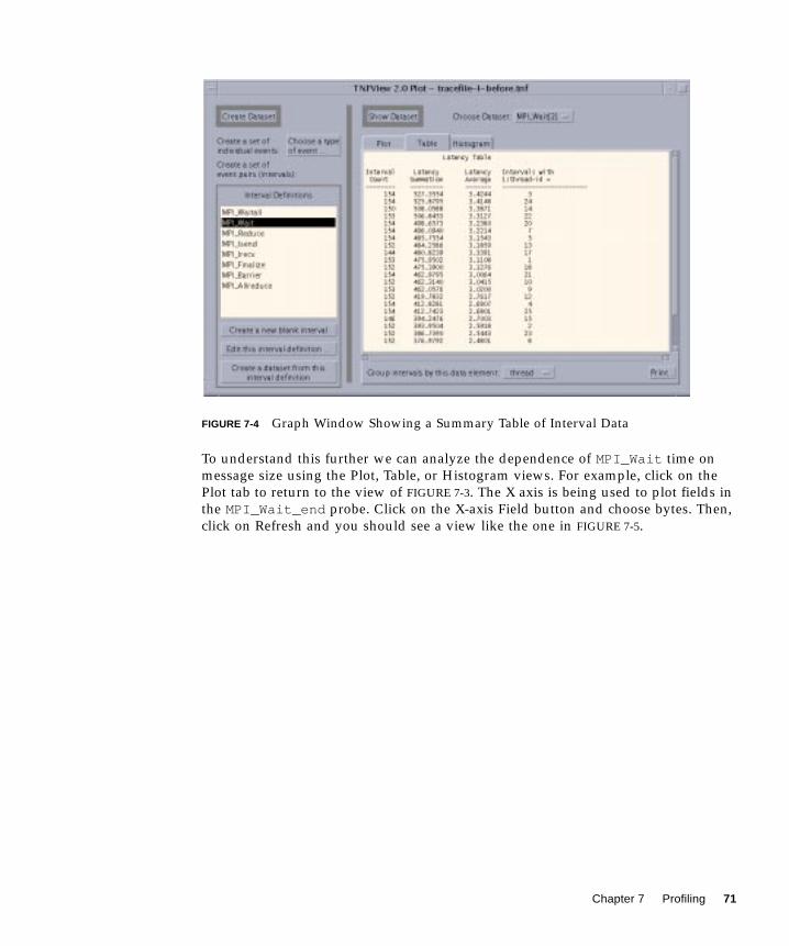
FIGURE 7-4 Graph Window Showing a Summary Table of Interval Data

To understand this further we can analyze the dependence of MPI_Wait time on

message size using the Plot, Table, or Histogram views. For example, click on the

Plot tab to return to the view of FIGURE 7-3. The X axis is being used to plot fields in

the MPI_Wait_end probe. Click on the X-axis Field button and choose bytes. Then,

click on Refresh and you should see a view like the one in FIGURE 7-5.


FIGURE 7-5 Scatter Plot of Time Spent in MPI_Wait as a Function of the Number of BytesReceived. Zero Bytes Indicate The Completion of a Send, Rather Than aReceive.

The byte counts on the X axis in FIGURE 7-5 are bytes received. In particular,

MPI_Wait calls that report zero bytes are completing nonblocking send operations.

The rest are completing nonblocking receive operations.

Note – In MPI, the number of bytes in a message is known on the sender’s side

when the send is posted and on the receiver’s side when the receive is completed

(rather than posted). Sun MPI’s TNF probes report the number of bytes in a message

in the same way. For example, a nonblocking send reports TNF byte information

with the MPI_Isend call while a nonblocking receive reports TNF byte information

with the MPI_Wait call. For more information on what information TNF arguments

report, see the Sun MPI Programming and Reference Guide.

We see from the figure that an appreciable amount of time is being spent waiting for

sends to complete. This is indicative of buffer congestion, which prevents senders

from writing their messages immediately into shared-memory buffers. We can

remedy this situation by rerunning the code with Sun MPI environment variables set

for large buffers.


FIGURE 7-5 shows that there are messages that are just over 40 Kbytes. To increase

buffering substantially past this size, we add

to our list of run-time environment variables. For further information about Sun MPI

environment variables, see Appendix C of this volume.

Finding Hotspots

Timings indicate that adding these new environment variables speeds the

benchmark up by 5 percent. This speedup is encouraging since our code spends only

20 percent of the time in MPI in the first place. In particular, the time spent on

MPI_Wait calls that terminate MPI_Isend calls has practically vanished.

Nevertheless, MPI_Wait continues to consume the most time of any MPI calls for

this job. Having rerun the job with larger MPI buffers, we may once again generate

a scatter plot of time spent in MPI_Wait calls (MPI_Wait latency) as a function of

elapsed time. Compare the new distribution shown in FIGURE 7-6 and with the one

shown in FIGURE 7-3. The new distribution shows that MPI_Wait times have

decreased dramatically. However, tall fingers of high-latency calls shoot up roughly

every 200 ms. These fingers are a symptom of message-passing traffic functioning as

global synchronizations. Indeed, these synchronizations occur as computation in this

three-dimensional application goes from x to y to z axis. This MPI time has little to

do with how fast MPI is moving data.

% setenv MPI_SHM_CPOOLSIZE 102400% setenv MPI_SHM_CYCLESTART 0x7fffffff


FIGURE 7-6 Scatter Plot of Time Spent in MPI_Wait as a Function of Elapsed Time,Running with Sun MPI Environment Variables That Relieve BufferCongestion

To study such a slowdown in detail, click on a high-latency point in the scatter plot.

This centers the cross-hairs back in the timeline view on the selected interval. Within

the timeline plot, you can navigate through a sequence of events using the tnfviewNavigate by... pull-down list, and left and right (previous and next) arrows. For

example, by pulling down Navigate by... and selecting current vid, you can restrict

navigation forward and backward on one particular MPI process. By using these

detailed navigation controls, you can confirm which sequence of MPI calls

characterize hot spots, or which interprocess dependencies are causing long

synchronization delays.


Second Prism Case Study – CollectiveOperationsOur first case study centered about point-to-point communications. Now, let us turn

our attention to one based on collective operations. We examine another popular

benchmark, which sorts sets of keys. The benchmark was run under the Prism

programming environment on a single, shared-memory node using 16 processes.

Once again, we begin by setting Sun MPI environment variables:

since we are interested in the performance of this benchmark as a dedicated job.

Synchronizing Skewed Processes: Timeline View

The message-passing part of the code involves a bucket sort, implemented with an

MPI_Allreduce , an MPI_Alltoall , and an MPI_Alltoallv , though no such

knowledge is required for effective profiling with the Prism programming

environment. Instead, running the code under the Prism environment, we quickly

see that the most time-consuming MPI calls are MPI_Alltoallv and

MPI_Allreduce . (See “Summary Statistics of MPI Usage” on page 69.) Navigating a

small section of the timeline window, we see a tight succession of MPI_Allreduce ,

MPI_Alltoall , and MPI_Alltoallv calls. One such iteration is shown in

FIGURE 7-7; we have shaded and labeled time-consuming sections.

% setenv MPI_SPIN 1% setenv MPI_PROCBIND 1


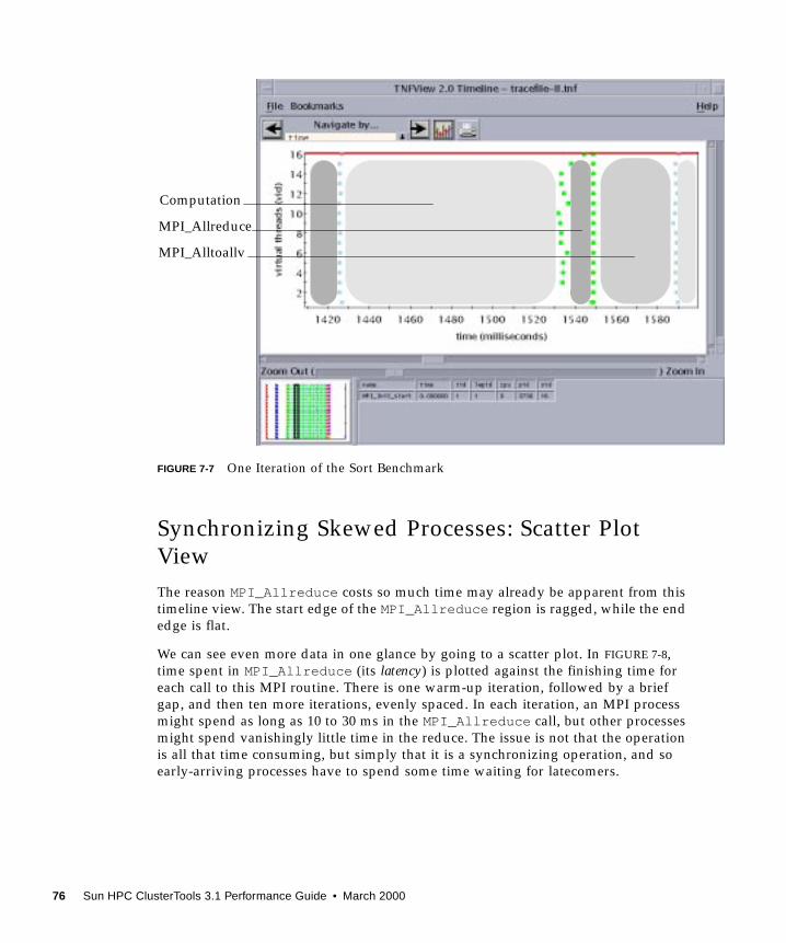
FIGURE 7-7 One Iteration of the Sort Benchmark

Synchronizing Skewed Processes: Scatter Plot

View

The reason MPI_Allreduce costs so much time may already be apparent from this

timeline view. The start edge of the MPI_Allreduce region is ragged, while the end

edge is flat.

We can see even more data in one glance by going to a scatter plot. In FIGURE 7-8,

time spent in MPI_Allreduce (its latency) is plotted against the finishing time for

each call to this MPI routine. There is one warm-up iteration, followed by a brief

gap, and then ten more iterations, evenly spaced. In each iteration, an MPI process

might spend as long as 10 to 30 ms in the MPI_Allreduce call, but other processes

might spend vanishingly little time in the reduce. The issue is not that the operation

is all that time consuming, but simply that it is a synchronizing operation, and so

early-arriving processes have to spend some time waiting for latecomers.

Computation

MPI_Alltoallv

MPI_Allreduce


FIGURE 7-8 Scatter Plot of MPI_Allreduce Latencies (x axis: MPI_Allreduce_end)

As in FIGURE 7-6, brief, well-defined instants of very high-latency message-passing

calls typically signal moments in code execution of considerable interprocess

synchronization.

The next MPI call is to MPI_Alltoall , but from our Prism profile we discover that

it occurs among well-synchronized processes (thanks to the preceding

MPI_Allreduce operation) and uses very small messages (64 bytes). It consumes

very little time.

Interpreting Performance Using Histograms

The chief MPI call is this case study is the MPI_Alltoallv operation. The processes

are still well synchronized, as we saw in FIGURE 7-7, but we learn from the Table

display that there are on average 2 Mbytes of data being sent or received per

process. Clicking on the Histogram tab, we get the view seen in FIGURE 7-9. There are

a few, high-latency outliers, which a scatter plot would indicate take place during

the first warm-up iteration. Most of the calls, however, take roughly 40 ms. The

effective bandwidth for this operation is therefore:

(2 Mbyte / process) * 16 processes / 40 ms = 800 Mbyte/second


Basically, each datum undergoes two copies (one to shared memory and one from

shared memory) and each copy entails two memory operations (a load and a store),

so this figure represents a memory bandwidth of 4 * 800 Mbyte/s = 3.2 Gbyte/s.

This benchmark was run on an HPC 6000 server, whose backplane is rated at 2.6

Gbyte/s. Our calculation is approximate, but it nevertheless indicates that we are

seeing saturation of the SMP backplane and we cannot expect to do much better

with our MPI_Alltoallv operation.

FIGURE 7-9 Histogram of MPI_Alltoallv Latencies

Performance Analysis TipsWhile Prism profiling can involve only a few mouse clicks, more advanced

techniques offer more sophisticated results.

Coping With Buffer Wraparound

Event-based profiling can collect a lot of data. TNF probe data collection employs

buffer wraparound, so that once a buffer file is filled the newer events will overwrite

older ones. Thus, final traces do not necessarily report events starting at the

beginning of a program and, indeed, the time at which events start to be reported


may vary slightly from one MPI process to another, depending on the amount of

probed activity on each process. Nevertheless, trace files will generally show

representative profiles of an application since newer, surviving events tend to

represent execution during steady state.

If buffer wraparound is an issue, then solutions include:

■ Scaling down the run (number of iterations or number of processes).

■ Using larger trace buffers.

■ Selective enabling of probes.

■ Profiling isolated sections of code by terminating jobs early.

Profiling isolated sections of code by modifying user source code.

Profiling isolated sections of code by isolating sections at run time.

Scaling Down the Run

You should usually perform code profiling and tuning on “stripped down” runs so

that many profiling experiments may be run. We describe these precautions in detail

at the beginning of this chapter.

Using Larger Trace Buffers.

To increase the size of trace buffers beyond the default value, use the Prism

command

(prism all) tnffile filename size

where size is the size in Kbytes of the trace buffer for each process. The default value

is 128 Kbytes. Larger values, such as 256, 512, or 1024, can sometimes prove more

useful.

By default, the Prism programming environment places trace buffers in /usr/tmpbefore they are merged into the user’s trace file. If this file partition is too small for

very large traces, you can redirect buffers to other directories using the

PRISM_TNFDIRenvironment variable. In order to minimize profile disruption

caused by writing very large trace files to disk, you should use local file systems

such as /usr/tmp and /tmp whenever possible instead of file systems that are

mounted over a network.

Note – While the Prism programming environment usually cleans up trace buffers

after the final merge, abnormal conditions could cause the Prism environment to

leave large files behind. Users who abort profiling sessions with large traces should

check /usr/tmp periodically for large, unwanted files.


Selectively Enabling Probes

You can focus data collection on the events that are most relevant to performance in

order either to reduce sizes of buffer files or to make profiling less intrusive. Prism

performance analysis can disturb an application’s performance characteristics, so

you should consider focusing data collection even if larger trace buffers are an

option.

TNF probes are organized in probe groups. For the TNF-instrumented version of the

Sun MPI library, the probe groups are structured as follows:

FIGURE 7-10 Sun MPI TNF Probe Groups

There are several probes that belong to both the mpi_request group and the

mpi_pt2pt group. For further information about probe groups, see the Sun MPIProgramming and Reference Guide.

For message-passing performance, typically the most important groups are:

■ mpi_pt2pt – point-to-point message passing

■ mpi_request – other probes for nonblocking point-to-point calls

■ mpi_coll – collectives

■ mpi_io_rw – file I/O

mpi_api

mpi_request

mpi_pt2pt

mpi_collmpi_commmpi_datatypesmpi_procmgmtmpi_topo

mpi_io

mpi_blkp2pmpi_nblkp2p

mpi_io_consistencympi_io_datarepmpi_io_errhandlermpi_io_filempi_io_rw

{

{{


Profiling Isolated Sections of Code — Terminating DataCollection Mid-Course

If you are especially interested in the steady-state performance characteristics of the

code, you might experiment with terminating a run early. If you choose to terminate

the run early, you will not spend time waiting for job completion when you already

have the profiling data you want. Further, by letting the job finish you risk the

possibility of uninteresting, post-processing steps overwriting the interesting steady-

state trace data.

To interrupt program execution, click on Interrupt, set a breakpoint, or use a Prism

command such as

sh sleep 200

to wait a prescribed length of time.

Then, turn off data collection and view the performance data. Once you have viewed

performance data, you cannot resume collecting data in the same run. However, you

can run your program to completion.

Profiling Isolated Sections of Code — From Within SourceCode

You can turn TNF data collection on and off within user source code, using the

routines tnf_process_disable , tnf_process_enable , tnf_thread_disable ,

and tnf_thread_enable . Since these are C functions, Fortran usage would require

added hints for the compiler, as follows:

Whether you call these functions from C or Fortran, you must then link with

–ltnfprobe . For more information, see the Solaris man pages on these functions.

Profiling Isolated Sections of Code — At Run Time

The Prism programming environment allows users to turn collection on and off

during program execution whenever execution is stopped: for example, with a break

point or by using the interrupt command.

call tnf_process_disable() !$pragma c(tnf_process_disable)call tnf_process_enable() !$pragma c(tnf_process_enable)call tnf_thread_disable() !$pragma c(tnf_thread_disable)call tnf_thread_enable() !$pragma c(tnf_thread_enable)


If the profiled section will be entered and exited many times, data collection may be

turned on and off automatically using tracepoints. Note that the term “trace” is used

now in a different context. For TNF use, a trace is a probe. For the Prism

programming environment and other debuggers, a tracepoint is a point where

execution stops and possibly an action takes place but, unlike a breakpoint, program

execution resumes after the action.

For example, if data collection should be turned on at line 128 but then off again at

line 223, you can specify

If you compiled and linked the application with high degrees of optimization, then

specification of line numbers may be meaningless. If you compiled and linked the

application without –g , then specifying numbers will not work. In such cases, you

can turn data collection on and off at entry points to routines using trace in routinesyntax, providing that those routines have not been inlined. For example:

Prism tracepoints have detectable effects on the behavior of the code being profiled.

The effects of the tracepoints can originate from:

■ Displaying a message when a tracepoint is encountered (modifying the event by

using the Prism Event Table can suppress such a message)

■ Making operating system calls

■ Synchronizing MPI processes

■ Responding to a breakpoint

■ Polling after a breakpoint

For this reason, you should not use trace commands inside inner loops, where they

would execute repeatedly, distorting your program’s performance. Use Prism

tracepoints to turn data collection on and off only around large amounts of code

execution.

(prism all) trace at 128 {tnfcollection on}(prism all) trace at 223 {tnfcollection off}

(prism all) trace in routine1 {tnfcollection on}(prism all) trace in routine2 {tnfcollection off}


Inserting TNF Probes Into User Code

While Sun HPC ClusterTools libraries have TNF probes for performance profiling,

user code probably will not. You can add probes manually, but since they are C

macros you can add them only to C and C++ code. To use TNF probes from Fortran

code, you must make calls to C code, such as in this C file, probes.c :

The start routine accepts a descriptive string, while the end routine takes a

double-precision operation count.

Then, using Fortran, you might write in main.f :

Note – Fortran will convert routine names to lowercase and append an underscore

character.

To compile and link, use:

% tmcc –c probes.c

% tmf77 main.f probes.o –lmpi –ltnfprobe

By default, the Prism command tnfcollection on enables all probes.

Alternatively, these sample probes could be controlled through their probe group

user_probes . Profile analysis can use the interval my_probe .

For more information on TNF probes, consult the man page for TNF_PROBE(3X).

#include <tnf/probe.h>void my_probe_start_(char *label_val) { TNF_PROBE_1(my_probe_start,”user_probes”,””, tnf_string,label,label_val);}void my_probe_end_ (double *ops_val) { TNF_PROBE_1(my_probe_end ,”user_probes”,””, tnf_double,ops,*ops_val);}

DOUBLE PRECISION OPERATION_COUNTOPERATION_COUNT = 2.D0 * NCALL MY_PROBE_START(“DOTPRODUCT”)XSUM = 0.D0DO I = 1, N

XSUM = XSUM + X(I) * Y(I)END DOCALL MY_PROBE_END(OPERATION_COUNT)


Collecting Data Batch Style

For more involved data collection experiments, you can collect TNF profiling

information in batch mode, for viewing and analysis in a later, interactive session.

Such collection may be performed using the commands-only mode of the Prism

environment, invoked with prism –C . For example, the simplest data collection

experiment would be

The wait command is needed to keep file merge from happening until after the

program has completed running. See the Prism User’s Guide for more information on

commands-only mode.

Accounting for MPI Time

Sometimes you will find it difficult to account for MPI activity. For example, if you

issue an nonblocking send or receive (MPI_Isend or MPI_Irecv ), the data

movement may occur during that call, during the corresponding MPI_Wait or

MPI_Test call, or during any other MPI call in between.

Similarly, general polling (such as with the environment variable MPI_POLLALL)

may skew accounting. For example, an incoming message may be read during a

send call because polling causes arrivals to be polled aggressively.

% prism -C -n 8 a.out << EOFtnfcollection ontnfenable mpi_pt2pttnfenable mpi_requesttnfenable mpi_colltnfenable mpi_io_rwrunwaitquitEOF


TNF Profiling Without Using the PrismEnvironmentBecause the Prism programming environment invokes TNF utilities to perform data

collection, you can profile MPI programs by invoking the TNF utilities directly

without using the Prism environment. However, bypassing the Prism environment

means that you forgo a number of ease-of-use facilities, such as representing process

timelines according to MPI rank. The Prism environment also reconciles timestamps

when a job is distributed over many nodes and uses multiple clocks that are not

synchronized with one another. Finally, because Prism processes may affect profiling

activity, there may be times when you want to bypass the Prism environment during

data collection.

Using prex

The utility to perform TNF data collection directly is prex . To enable all probes,

place the following commands in your .prexrc file. (Note the leading “.” in the file

name).

Then, remove old buffer files, run prex , and merge the data, as shown below. You

can view the final output file, a.tnf , under the Prism environment.

Because prex does not correct for the effects of clock skew, it is useful only for MPI

programs running on individual SMPs. Also, data collected by prex does not

identify MPI ranks in the data—if you attempt to display prex data in tnfview , the

VIDs (ranks) will be displayed in random order.

enable $alltrace $allcontinue

% rm /tmp/trace-* If you are running CRE:% mprun -np 4 prex -s 128 a.out If you are running LSF:% bsub -I -n 4 prex -s 128 a.out Then:% /opt/SUNWhpc/bin/sparcv7/tnfmerge -o a.tnf /tmp/trace-*


For more information on prex , see its Solaris man page.

Using the tnfdump Utility

You can implement custom post-processing of TNF data using the tnfdump utility,

which converts TNF trace files, such as the one produced by the Prism programming

environment, into an ASCII listing of timestamps, time differentials, events, and

probe arguments.

To use this command, specify

% tnfdump filename

where filename is the name of the TNF trace data file produced by the Prism

programming environment.

The resulting ASCII listing, produced on the standard output, can be several times

larger than the tracefile and may require a wide window for viewing. Nevertheless,

it is full of valuable information.

For more information about the tnfdump command, see the tnfdump (1) man page.

Profiling Without Using the PrismEnvironment or TNF UtilitiesBoth MPI and the Solaris enviroment offer useful profiling facilities. Using the MPI

profiling interface, you can investigate MPI calls. Using your own timer calls, you

can profile specific behaviors. Using the Solaris gprof utility, you can profile diverse

multiprocess codes, including those using MPI.

Using the MPI Profiling Interface

The MPI standard supports a profiling interface, which allows any user to profile

either individual MPI calls or the entire library. This interface supports two

equivalent APIs for each MPI routine. One has the prefix MPI_, while the other has

PMPI_. User codes typically call the MPI_ routines. A profiling routine or library

will typically provide wrappers for the MPI_ APIs that simply call the PMPI_ ones,

with timer calls around the PMPI_ call.


You may use this interface to change the behavior of MPI routines without

modifying your source code. For example, suppose you believe that most of the time

spent in some collective call such as MPI_Allreduce is due to the synchronization

of the processes that is implicit to such a call. Then, you might compile a wrapper

such as the one shown below, and link it into your code before

–lmpi . The effect will be that time profiled by MPI_Allreduce calls will be due

exclusively to the MPI_Allreduce operation, with synchronization costs attributed

to barrier operations.

Profiling wrappers or libraries may be used even with application binaries that have

already been linked. See the Solaris man page for ld for more information on the

environment variable LD_PRELOAD.

You can get profiling libraries from independent sources for use with Sun MPI.

Typically, their functionality is rather limited compared to that of the Prism

environment with TNF, but for certain applications their use may be more

convenient or they may represent useful springboards for particular, customized

profiling activities. An example of a profiling library is included in the

multiprocessing environment (MPE) from Argonne National Laboratory. Several

external profiling tools can be made to work with Sun MPI using this mechanism.

For more information on this library and on the MPI profiling interface, see the SunMPI Programming and Reference Guide.

Inserting MPI Timer Calls

Sun HPC ClusterTools implements the Sun MPI timer call MPI_Wtime(demonstrated in the example below) with the high-resolution timer gethrtime. If

you use MPI_Wtime calls, you should use them to measure sections that last more

than several microseconds. Times on different processes are not guaranteed to be

synchronized. For information about gethrtime, see the gethrtime(3C) man

page.

When profiling multiprocess codes, you need to ensure that the timings are not

distorted by the asynchrony of the various processes. For this purpose, you usually

need to synchronize the processes before starting and before stopping the timer.

subroutine MPI_Allreduce(x,y,n,type,op,comm,ier)integer x(*), y(*), n, type, op, comm, iercall PMPI_Barrier(comm,ier)call PMPI_Allreduce(x,y,n,type,op,comm,ier)end


In the following example, most processes may accumulate time in the interesting,

timed portion, waiting for process 0 (zero) to emerge from uninteresting

initialization. This would skew your program’s timings. For example:

When stopping a timer, remember that measurements of elapsed time will differ on

different processes. So, execute another barrier before the “stop” timer. Alternatively,

use “maximum” elapsed time for all processes.

Avoid timing very small fragments of code. This is good advice when debugging

uniprocessor codes, and the consequences are greater with many processors. Code

fragments perform differently when timed in isolation. The introduction of barrier

calls for timing purposes can be disruptive for short intervals.

Using gprof

The Solaris utility gprof may be used for multiprocess codes, such as those that use

MPI. It can be helpful for profiling user routines, which are not automatically

instrumented with TNF probes by Sun HPC ClusterTools software. Several points

should be noted:

■ Compile and link your programs with –pg (Fortran) or –xpg (C).

■ Use the environment variable PROFDIRto profile multiprocess jobs, such as those

that use MPI.

■ Use the gprof command after program execution to gather summary statistics

either on individual processes or for multiprocess aggregates.

■ gprof does not profile MPI libraries. Hence, any time your program spends

within the Sun MPI layer (such as waiting for buffers to be freed) will not appear

in gprof profiles. However, gprof may record time your program spends in Sun

MPI’s lower-level. Notably, gprof may display on-node data transfers as memcpycalls and transfers between nodes as read and write calls. Time spent waiting

for messages or buffers may appear as poll , yield , or thr_yield calls.

■ gprof will not recognize relationships between process ids, used to tag profile

files, and MPI process ranks.

CALL MPI_COMM_RANK(MPI_COMM_WORLD,ME,IER)IF ( ME .EQ. 0 ) THEN initializationEND IF! place barrier here! CALL MPI_BARRIER(MPI_COMM_WORLD, IER)T_START = MPI_WTIME() timed portionT_END = MPI_WTIME()


■ gprof profiles from different processes may overwrite one another if a

multiprocess job spans multiple nodes.

For more information about gprof , see the gprof man page.

The Prism and gprof profiling methods are incompatible, although complementary.



APPENDIX A

Summary of Performance Tips

This appendix summarizes key performance tips found in this document. They are

organized under the following categories:

■ “Compilation and Linking” on page 91

■ “Sun MPI Environment Variables” on page 92

■ “Job Launch on a Multinode Cluster” on page 93

■ “MPI Programming Tips” on page 95

■ “Prism Profiling” on page 96

Compilation and LinkingSee Chapter 5 for details.

■ Use the mpf77 , mpf90 , mpcc, and mpCCutilities where possible:

See “Using the mp* Utilities” on page 45.

■ For 64-bit binaries, use –xarch=v9a .

See “–xarch ” on page 47.

■ For Fortran programs:

■ To suppress verbose numerical warnings, link in

% mpf77 –fast –xarch=v8plusa –fsimple=2 –o a.out a.f –lmpi% mpcc –fast –xarch=v8plusa –fsimple=2 –o a.out a.c –lmpi –lmopt

SUBROUTINE IEEE_RETROSPECTIVE()END

91

■ Starting with the Sun WorkShop 5.0 release of the compilers, consider

–xvector

–xprefetch

■ Consider using –stackvar .

See “mpf77 –fast and IEEE warnings” on page 46 and “Other Issues” on page

48.

■ For C programs:

■ Consider using –xrestrict .

■ Starting with the Sun WorkShop 5.0 release of the compilers, consider using

–xprefetch .

See “Other Issues” on page 48.

■ For Sun S3L:

■ Use –ls3l (–lmpi is then unnecessary).

■ Use the most recent version of the Sun WorkShop compilers for superior

performance of Sun Performance Library.

See “Using the mp* Utilities” on page 45 and “Other Issues” on page 48.

Sun MPI Environment VariablesThe Sun MPI environment variables are discussed in Chapter 6 and Appendix C.

■ Especially if you will leave at least one idle processor per node to service system

daemons, consider using

% setenv MPI_SPIN 1

See “Are You Running on a Dedicated System?” on page 51.

■ If there are no other MPI jobs running and your job is single-threaded,

% setenv MPI_PROCBIND 1

See “Are You Running on a Dedicated System?” on page 51.

■ Suppress cyclic message passing with


or, in a 64-bit environment, with

% setenv MPI_SHM_CYCLESTART 0x7fffffffffffffff

See “Suppress Cyclic Messages” on page 51.

■ If system buffers are used “safely” (that is, code does not rely on unlimited

buffering to avoid deadlock)


% setenv MPI_POLLALL 0

If this setting causes your code to deadlock, try using larger buffers, as noted in

the next bullet.

See “Does the Code Use System Buffers Safely?” on page 52.

■ If you are willing to trade memory for performance, increase buffering with



See “Are You Willing to Trade Memory for Performance?” on page 52.

■ Move certain “warm-up” effects to MPI_Init() with

% setenv MPI_WARMUP 1


This smooths performance profiles and speeds certain portions of code, but

MPI_Init() can take up to minutes.

See “Initializing Sun MPI Resources” on page 54.

■ If more runtime diagnostic information is desired,

% setenv MPI_PRINTENV 1

% setenv MPI_SHOW_INTERFACES 3

% setenv MPI_SHOW_ERRORS 1

See “Is More Runtime Diagnostic Information Needed?” on page 55.

Job Launch on a Multinode Cluster

Checking Load

See “Running on a Dedicated System” on page 49.

CRE LSF UNIX

How high is the load? % mpinfo –N % lsload % uptime

What is causing the load? % mpps –e % bjobs –u all % ps –e

Appendix A Summary of Performance Tips 93

Objectives for Job Launch■ Minimize internode communication.

■ Run on one node if possible.

■ Place heavily communicating processes on the same node as one another.

See “Minimizing Communication Costs” on page 55.

■ Maximize bisection bandwidth.

■ Run on one node if possible.

■ Otherwise, spread over many nodes.

■ For example, spread jobs that use multiple I/O servers.

See “Bisection Bandwidth” on page 56.

Examples of Job Launch With the CRE■ To run 32 processes, with each block of consecutive 4 processes mapped to a

node:

% mprun –np 32 –Zt 4 a.out

or

% mprun –np 32 –Z 4 a.out

See “Collocal Blocks of Processes” on page 60.

■ To run 16 processes, with no two mapped to the same node:

% mprun –Ns –np 16 a.out

See “Multithreaded Job” on page 58.

■ To map 32 processes in round-robin fashion to the nodes in the cluster, with

possibly multiple processes per node:

% mprun –Ns –W –np 32 a.out

See “Round-Robin Distribution of Processes” on page 59.

■ To map the first 4 processes to node0 , the next 4 to node1 , and the next 8 to

node2 :

% cat nodelist

node0 4

node1 4

node2 8

% mprun –np 16 –Mf nodelist a.out

See “Detailed Mapping” on page 59.


Examples of Job Launch With LSF

See “Examples of Job Launch on a Multinode Cluster Under LSF” on page 60.

■ To run 32 processes, with each block of consecutive 4 processes run on a distinct

node:


■ To map 32 processes in a round-robin fashion on 4 distinct nodes:


MPI Programming Tips■ Minimize number and volume of messages.

See “Reduce the Number and Volume of Messages” on page 20.

■ Minimize synchronizations:

■ Generally reduce the amount of message passing.

■ Reduce the amount of explicit synchronization (such as MPI_Barrier() ,

MPI_Ssend() , and so on).

■ Post sends well ahead of when a receiver needs data.

■ Ensure sufficient system buffering.

See “Synchronization” on page 20.

■ Pay attention to buffering:

■ MPI specification does not guarantee buffering for standard sends

(MPI_Send() ).

■ Tune Sun MPI environment variables at run time to increase system buffering

(see Appendix C).

■ MPI buffered sends can entail extra copies.

See “Buffering” on page 21.

■ Pay attention to polling:

■ Match message-passing calls (receives to sends, collectives to collectives, and

so on).

■ Post MPI_Irecv() calls ahead of arrivals.

■ Avoid MPI_ANY_SOURCE.

■ Avoid MPI_Probe() and MPI_Iprobe() .

■ Set the environment variable MPI_POLLALL to 0 at run time.

See “Polling” on page 22.


■ Take advantage of MPI collective operations.

See “Sun MPI Collectives” on page 22.

■ Use contiguous data types:

■ Send some unnecessary padding if necessary.

■ Pack your own data if you can outperform generalized MPI_Pack() /

MPI_Unpack() routines.

See “Contiguous Data Types” on page 23.

■ Avoid congestion if you’re going to run over TCP:

■ Avoid “hot receivers.”

■ Use blocking point-to-point communications.

■ Use synchronous sends (MPI_Ssend() and related calls).

■ Use MPI collectives such as MPI_Alltoall() , MPI_Alltoallv() ,

MPI_Gather() , or MPI_Gatherv() , as appropriate.

■ At run time, set MPI_EAGERONLYto 0, and possibly lower

MPI_TCP_RENDVSIZE.

See “Special Considerations for Message Passing Over TCP” on page 23.

Prism ProfilingThe Prism environment offers ease of use with its MPI Performance Analysis. If you

accept the default values, Prism’s TNF profiling:

■ Requires no special compilation or linking.

■ Requires no special invocation.

■ Operates with a few mouse clicks.

Prism Profiling is discussed in Chapter 7 “Profiling” and in the Prism 6.1 User’sGuide.

▼ To Launch a Basic Profiling Session

Although Prism profiling supports detailed control of data collection and analysis,

you can launch a basic profiling session with only three commands.


● Use the following sequence of commands or menu entries:

■ Prism’s TNF browser (tnfview ) opens with a timeline view of your profiling

data.

■ Note how the events in the window represent elapsed time.

■ Inspect the representation for any obvious structure indicating interprocess

synchronization or program behavior.

■ Middle-drag the mouse to zoom the timeline view.

See “To Collect Performance Data” on page 67. Launching Prism profiling sessions is

discussed in detail in Chapter 6 of the Prism 6.1 User’s Guide.

▼ To Display Profiling Statistics

1. Click on the graph icon in the timeline window to open the graph window.

MPI calls appear on the list of Interval Definitions.

2. Identify the MPI calls that consume the most time and what fraction of overalltime they account for.

1. Click on a routine under Interval Definitions.

2. Click on Create a dataset from this interval definition.

3. Click on the Table tab.

4. Note the time spent under Latency Summation.

5. Repeat steps 1, 2, and 4 for other interesting MPI calls.

3. Identify the largest message sizes and which message sizes are responsible for themost time.

The TNF browser displays byte counts as bytes, sendbytes, or recvbytes. The TNF

browser reports byte counts in _start or _end probes. The TNF browser’s byte

counts for MPI_Wait or MPI_Test calls are bytes received (zero bytes usually

indicate completions of asynchronous sends).

1. Click on the the Plot tab—Select values under X axis, Y axis, and Field:, then click

on Refresh.

Step Prism Command Menu : Menu Entry

1 tnfcollection on Performance : Collection

2 run Execute : Run

3 tnfview Performance : Display TNF Data


2. Click on the Table tab—Select values under Group intervals by this data element:

(note that the browser may display the last column in hexadecimal format).

3. Click on the Histogram tab—Select values under Metric and Field:, then click on

Refresh

See “Summary Statistics of MPI Usage” on page 69.

▼ To Find Hotspots

1. Click on the Plot tab.

2. Click on a high-latency event to center the timeline view about a hotspot.

3. Return to the timeline view.

4. Navigate about the hotspot using the navigation buttons.

1. Open the Navigate by list and select current vid.

2. Click on the arrow icons to move forward and backward.

3. Read data about selected events in the Event Table.

See “Finding Hotspots” on page 73.

▼ To Control the Volume of Profiling Data

● Consider the following guidelines:

■ Scale down the run (reduce the number of iterations or the number of processes).

■ Use larger trace buffers.

■ Selectively enable probes.

■ Profile isolated sections of code by terminating jobs early, by modifying user

source code, or by isolating sections at run time.

See “Performance Analysis Tips” on page 78.


APPENDIX B

Sun MPI Implementation

This appendix discusses various aspects of the Sun MPI implementation.

The Sun MPI implementation can cause running processes to yield or deschedule if

they are idly waiting for messages. Typically, this is best when there is a heavy, time-

shared, multiuser load, but for best performance on a dedicated job you should keep

processes running.

The Sun MPI progress engine can advance multiple messages at once, supporting

MPI nonblocking point-to-point message passing.

Within a cluster of multiprocessor nodes, the Sun MPI library will take advantage of

high-speed shared memory mechanisms for messages between processes on the

same node. Between processes on different nodes, the Sun MPI library can use

remote shared memory (RSM) over Scalable Coherent Interface (SCI) networks,

providing latencies that are almost comparable to those realized over shared

memory. Otherwise, Sun MPI is still able to support message passing traffic between

any two nodes that have an TCP connection. The performance characteristics of

these three protocols vary.

Over shared memory and remote shared memory, Sun MPI uses sets of buffers to

stage messages between processes and postboxes to control the buffers. Typically,

each sender-receiver pair, known as a connection, has its own such resources

devoted to it. Messages will usually be pipelined, so that one process can start

receiving a message even while its partner is still sending. Sun MPI also supports a

special cyclic mode, in which large messages cycle within a fixed footprint of the

buffer area, allowing messages of unlimited size but adding extra synchronization

between the processes.

These aspects of the Sun MPI implementation are described here. Many of the

characteristics can be tuned at run time with environment variables, as discussed in

Appendix C.

99

Yielding and DeschedulingIn many programs, too much time in MPI routines is spent waiting for particular

conditions, such as the arrival of incoming data or the availability of system buffers.

Busy waiting costs computational resources, which could be better spent servicing

other users’ jobs or necessary system daemons.

Sun MPI has a variety of provisions for mitigating the effects of busy waiting. This

allows MPI jobs to run more efficiently, even when the load of a cluster node exceeds

the number of processors it contains. Two methods of avoiding busy waiting are

yielding and descheduling:

■ Yielding – A Sun MPI process can yield its processor with a Solaris system call if it

waits busily too long.

■ Descheduling – Alternatively, a Sun MPI process can deschedule itself. In

descheduling, a process registers itself with the “spin daemon” (spind ), which

will poll for the gating condition on behalf of the process. This is less resource

consuming than having the process poll, since the spind daemon can poll on

behalf of multiple processes. The process will once again be scheduled either if

the spind daemon wakes the process in response to a triggering event, or if the

process restarts spontaneously according to a preset timeout condition.

Yielding is less disruptive to a process than descheduling, but descheduling helps

free resources for other processes more effectively. As a result of these policies,

processes that are tightly coupled can become coscheduled. Yielding and

coscheduling can be tuned with Sun MPI environment variables, as described in

Appendix C.

Progress EngineWhen a process enters an MPI call, Sun MPI may act on a variety of messages. Some

of the actions and messages may not pertain to the call at all, but may relate to past

or future MPI calls.


To illustrate, consider the code sequence

Sun MPI behaves as one would expect. That is, the computational portion of the

program is interrupted to perform MPI blocking send operations, as illustrated in

FIGURE B-1.

FIGURE B-1 Blocking Sends Interrupt Computation

Now, consider the code sequence

In this case, the nonblocking receive operation conceptually overlaps with the

intervening computation, as in FIGURE B-2.

computationCALL MPI_SEND()computationCALL MPI_SEND()computationCALL MPI_SEND()computation

computationCALL MPI_IRECV(REQ)computationCALL MPI_WAIT(REQ)computation

Appendix B Sun MPI Implementation 101

FIGURE B-2 Conceptually, nonblocking operations overlap with computation.

In fact, however, progress on the nonblocking receive is suspended from the time the

MPI_Irecv() returns until the instant Sun MPI is once again invoked, with the

MPI_Wait() . There is no actual overlap of computation and communication, and

the situation is as depicted in FIGURE B-3.

FIGURE B-3 Computational resources are devoted either to user computation or to MPIoperations, but not both at once.


Nevertheless, reasonably good overlap between computation and nonblocking

communication can be realized, since the Sun MPI library is able to progress a

number of message transfers within one MPI call. Consider the code sequence

which combines the previous examples. Now, there is effective overlap of

computation and communication, because the intervening, blocking sends also

progress the nonblocking receive, as depicted in FIGURE B-4. The performance payoff

is not due to computation and communication happening at the same time. Indeed,

a CPU still only computes or else moves data — never both at the same time. Rather,

the speedup results because scheduling of computation with the communication of

multiple messages is better interwoven.

FIGURE B-4 Progress may be made on multiple messages by a single MPI call, even if thatcall does not explicitly reference the other messages.

In general, when Sun MPI is used to perform a communication call, a variety of

other activities may also take place during that call, as we have just discussed.

Specifically,

computationCALL MPI_IRECV(REQ)computationCALL MPI_SEND()computationCALL MPI_SEND()computationCALL MPI_SEND()computationCALL MPI_WAIT(REQ)computation


1. A process may progress any outstanding, nonblocking sends, depending on the

availability of system buffers.

2. A process may progress any outstanding, nonblocking receives, depending on the

availability of incoming data.

3. A process may generally poll for any messages whatsoever, to drain system

buffers.

4. A process must periodically watch for message cancellations from other processes

in case another process issues an MPI_Cancel() call for a send.

5. A process may choose to yield its computational resources to other processes if no

useful progress is being made.

6. A process may choose to deschedule itself, if no useful progress is being made.

A nonblocking MPI communication call will return whenever there is no progress to

be made. For example, system buffers may be too congested for a send to proceed, or

there may not yet be any more incoming data for a receive.

In contrast, a blocking MPI communication call may not return until its operation

has completed, even when there is no progress to be made. Such a call will

repeatedly try to make progress on its operation, also checking all outstanding

nonblocking messages for opportunities to perform constructive work (items 1–4

above). If these attempts prove fruitless, the process will periodically yield its CPU

to other processes (item 5). After multiple yields, the process will attempt to

deschedule itself via the spind daemon (item 6).

Shared-Memory Point-to-Point MessagePassingSun MPI uses a variety of algorithms for passing messages from one process to

another over shared memory. The characteristics of the algorithms as well as the

ways in which algorithms are chosen at run time can largely be controlled by Sun

MPI environment variables, which are described in Appendix C. This section

describes the background concepts.


Postboxes and Buffers

For on-node, point-to-point message passing, the sender writes to shared memory

and the receiver reads from there. Specifically, the sender writes a message into

shared-memory buffers, depositing pointers to those buffers in shared-memory

postboxes. As soon as the sender finishes writing any postbox, that postbox, along

with any buffers it points to, may be read by the receiver. Thus, message passing is

pipelined — a receiver may start reading a long message even while the sender is

still writing it.

FIGURE B-5 depicts this behavior. The sender moves from left to right, using the

postboxes consecutively. The receiver follows. The buffers F, G, H, I, J, K, L, and M

are still “in flight” between sender and receiver and they appear out of order.

Pointers from the postboxes are required to keep track of the buffers. Each postbox

can point to multiple buffers, and the case of two buffers per postbox is illustrated

here.

FIGURE B-5 Snapshot of a pipelined message. Message data is buffered in the labeledareas.


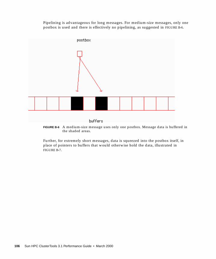
Pipelining is advantageous for long messages. For medium-size messages, only one

postbox is used and there is effectively no pipelining, as suggested in FIGURE B-6.

FIGURE B-6 A medium-size message uses only one postbox. Message data is buffered inthe shaded areas.

Further, for extremely short messages, data is squeezed into the postbox itself, in

place of pointers to buffers that would otherwise hold the data, illustrated in

FIGURE B-7.


FIGURE B-7 A short message squeezes data into the postbox and does not use any buffers.Message data is buffered in the shaded area.

For very long messages, it may be desirable to keep the message from overrunning

the shared-memory area. In that limit, the sender is allowed to advance only one

postbox ahead of the receiver. Thus, the footprint of the message in shared memory

is limited to at most two postboxes at any one time, along with associated buffers.

Indeed, the entire message is cycled through two fixed sets of buffers. FIGURE B-8 and

FIGURE B-9 show two consecutive snapshots of the same cyclic message. The two sets

of buffers, through which all the message data is being cycled, are labeled X and Y.

The sender remains only one postbox ahead of the receiver.


FIGURE B-8 First snapshot of a cyclic message. Message data is buffered in the labeledareas.


FIGURE B-9 Second snapshot of a cyclic message. Message data is buffered in the labeledareas.

Connection Pools Vs. Send-Buffer Pools

In the following example, we consider n processes that are collocal to a node.

A connection is a sender-receiver pair. Specifically, for n processes, there are n x (n–

1) connections. That is, A sending to B uses a different connection than B sending to

A, and any process sending to itself is handled separately.


Each connection has its own set of postboxes. For example, in FIGURE B-10, there are

two unidirectional connections for each pair of processes. There are 5x4=20

connections in all for the 5 processes. Each connection has shared-memory resources,

such as postboxes, dedicated to it. The shared-memory resources available to one

sender are shown.

FIGURE B-10 Shared-memory resources that are dedicated per connection includepostboxes and, optionally, buffer pools. The shared-memory resourcesavailable to one sender are shown.

By default, each connection also has its own pool of buffers. Users may override the

default use of connection pools, however, and cause buffers to be collected into npools, one per sender, with buffers shared among a sender’s n–1 connections. An

illustration of n send-buffer pools is shown in FIGURE B-11. The send-buffer pool

available to one sender is shown.


FIGURE B-11 Shared-memory resources per sender — for example, send-buffer pools. Thesend-buffer pool available to one sender is shown.

Eager Vs. Rendezvous

Another issue in passing messages is the use of the rendezvous protocol. By default,

a sender will be eager and try to write its message without explicitly coordinating

with the receiver (FIGURE B-12). Under the control of environment variables, Sun MPI

can employ rendezvous for long messages. Here, the receiver must explicitly

indicate readiness to the sender before the message can be sent, as seen in

FIGURE B-13.

To force all connections to be established during initialization, set the

MPI_FULLCONNINIT environment variable:



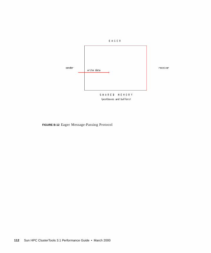
FIGURE B-12 Eager Message-Passing Protocol


FIGURE B-13 Rendezvous Message-Passing Protocol

Performance Considerations

The principal performance consideration is that a sender should be able to deposit

its message and complete its operation without coordination with any other process.

A sender may be kept from immediately completing its operation if:

■ Rendezvous is in force. (Rendezvous is suppressed by default.)

■ The message is being sent cyclically. This behavior can be suppressed by setting

MPI_SHM_CYCLESTARTvery high — for example,


■ The shared-memory resources (either buffers or postboxes) are temporarily

congested. Shared-memory resources can be increased by setting Sun MPI

environment variables at run time to handle any burst of message-passing

activity.

Using send-buffer pools rather than connection pools helps pool buffer resources

among a sender’s connections. For a fixed total amount of shared memory, this can

deliver effectively more buffer space to an application, improving performance.

Multithreaded applications can suffer, however, since a sender’s threads would

contend for a single send-buffer pool instead of for (n–1) connection pools.


Rendezvous protocol tends to slow performance of short messages, not only because

extra handshaking is involved, but especially because it makes a sender stall if a

receiver is not ready. Long messages can benefit, however, if there is insufficient

memory in the send-buffer pool or if their receives are posted in a different order

than they are sent.

Pipelining can roughly double the point-to-point bandwidth between two processes.

It may have little or no effect on overall application performance, however, if

processes tend to get considerably out of step with one another or if the nodal

backplane becomes saturated by multiple processes exercising it at once.

Full Vs. Lazy ConnectionsSun MPI, in default mode, starts up connections between processes on different

nodes only as needed. For example, if a 32-process job is started across four nodes,

eight processes per node, then each of the 32 processes has to establish 32–8=24

remote connections for full connectivity. If the job relied only on nearest-neighbor

connectivity, however, many of these 32x24=768 remote connections would be

unneeded.

On the other hand, when remote connections are established on an “as needed”

basis, startup is less efficient than when they are established en masse at the time of

MPI_Init() .

Timing runs typically exclude warmup iterations and, in fact, specifically run several

untimed iterations to minimize performance artifacts in start-up times. Hence, both

full and lazy connections perform equally well for most interesting cases.

RSM Point-to-Point Message PassingSun MPI supports high-performance message passing over remote shared memory

(RSM), running over Scalable Coherent Interface (SCI) networks. Aside from the

high-performance specifications of SCI, Sun MPI over RSM attains:

■ Low latency from bypassing the operating system

■ High bandwidth from striping messages over multiple channels

The RSM protocol has some similarities with the shared memory protocol, but it also

differs substantially, and environment variables are used differently.

Messages are sent over RSM in one of two fashions:


■ Short messages are fit into multiple postboxes and no buffers are used.

■ Pipelined messages are sent in 1024-byte buffers under the control of multiple

postboxes.

Short-message transfer is illustrated in FIGURE B-14. The first 23 bytes of a short

message are sent in one postbox, and 63 bytes are sent in each of the subsequent

postboxes. No buffers are used. For example, a 401-byte message travels as

23+63+63+63+63+63+63=401 bytes and requires 7 postboxes.

FIGURE B-14 A short RSM message. Message data is buffered in the shaded areas.

Pipelining is illustrated in FIGURE B-15. Postboxes are used in order, and each postbox

points to multiple buffers.

FIGURE B-15 A pipelined RSM message. Message data is buffered in the shaded areas.



APPENDIX C

Sun MPI Environment Variables

This section describes some Sun MPI environment variables in greater detail.

Prescriptions for using these variables for performance tuning are provided in

Chapter 6, and additional information on these environment variables in general can

be found in the Sun MPI Programming and Reference Guide.

These environment variables are closely related to the details of the Sun MPI

implementation, and their use requires an understanding of the implementation.

More details on the Sun MPI implementation can be found in Appendix B.

Yielding and DeschedulingA blocking MPI communication call may not return until its operation has

completed. If the operation has stalled, perhaps because there is insufficient buffer

space to send or because there is no data ready to receive, Sun MPI will attempt to

progress other outstanding, nonblocking messages. If no productive work can be

performed, then in the most general case Sun MPI will yield the CPU to other

processes, ultimately escalating to the point of descheduling the process via the

spind daemon.

Setting MPI_COSCHED=0 specifies that processes should not be descheduled. This is

the default behavior.

Setting MPI_SPIN =1 suppresses yields. The default value, 0, allows yields.

117

PollingBy default, Sun MPI polls generally for incoming messages, regardless of whether

receives have been posted. To suppress general polling, use MPI_POLLALL=0.

Shared-Memory Point-to-Point MessagePassingThe size of each shared-memory buffer is fixed at 1 Kbyte. Most other quantities in

shared-memory message passing are settable with MPI environment variables.

For any point-to-point message, Sun MPI will determine at run time whether the

message should be sent via shared memory, remote shared memory, or TCP. The

flowchart in FIGURE C-1 illustrates what happens if a message of B bytes is to be sent

over shared memory.

FIGURE C-1 Message of B Bytes Sent Over Shared Memory

For pipelined messages, MPI_SHM_PIPESIZE bytes are sent under the control of any

one postbox. If the message is shorter than 2 x MPI_SHM_PIPESIZE bytes, the

message is split roughly into halves.


For cyclic messages, MPI_SHM_CYCLESIZEbytes are sent under the control of any

one postbox, so that the footprint of the message in shared memory buffers is 2 x

MPI_SHM_CYCLESIZEbytes.

The postbox area consists of MPI_SHM_NUMPOSTBOXpostboxes per connection.

By default, each connection has its own pool of buffers, each pool of size

MPI_SHM_CPOOLSIZEbytes.

By setting MPI_SHM_SBPOOLSIZE, users may specify that each sender has a pool of

buffers, each pool having MPI_SHM_SBPOOLSIZEbytes, to be shared among its

various connections. If MPI_SHM_CPOOLSIZEis also set, then any one connection

may consume only that many bytes from its send-buffer pool at any one time.

Memory Considerations

In all, the size of the shared-memory area devoted to point-to-point messages is

n x ( n – 1 ) x ( MPI_SHM_NUMPOSTBOXx ( 64 + MPI_SHM_SHORTMSGSIZE) +

MPI_SHM_CPOOLSIZE)

bytes when per-connection pools are used (that is, when MPI_SHM_SBPOOLSIZEisnot set), and

n x ( n – 1 ) x MPI_SHM_NUMPOSTBOXx ( 64 + MPI_SHM_SHORTMSGSIZE) + n x

MPI_SHM_SBPOOLSIZE

bytes when per-sender pools are used (that is, when MPI_SHM_SBPOOLSIZEis set).

Cyclic message passing limits the size of shared memory that is needed to transfer

even arbitrarily large messages.


A sender should be able to deposit its message and complete its operation without

waiting for any other process. You should typically:

■ Use the default setting of MPI_EAGERONLY, or set MPI_SHM_RENDVSIZEto be

larger than the greatest number of bytes any on-node message will have.

■ Increase MPI_SHM_CYCLESTARTso that no messages will be sent cyclically.

■ Increase MPI_SHM_CPOOLSIZEto ensure sufficient buffering at all times.

In theory, rendezvous can improve performance for long messages if their receives

are posted in a different order than their sends. In practice, the right set of

conditions for overall performance improvement with rendezvous messages is rarely

met.

Appendix C Sun MPI Environment Variables 119

Send-buffer pools can be used to provide reduced overall memory consumption for

a particular value of MPI_SHM_CPOOLSIZE. If a process will only have outstanding

messages to a few other processes at any one time, then set MPI_SHM_SBPOOLSIZEto the number of other processes times MPI_SHM_CPOOLSIZE. Multithreaded

applications might suffer, however, since then a sender’s threads would contend for

a single send-buffer pool instead of for multiple, distinct connection pools.

Pipelining, including for cyclic messages, can roughly double the point-to-point

bandwidth between two processes. This is a secondary performance effect, however,

since processes tend to get considerably out of step with one another, and since the

nodal backplane can become saturated with multiple processes exercising it at the

same time.

Restrictions■ The short-message area of a postbox must be large enough to point to all the

buffers it commands. In practice, this restriction is relatively weak since, if the

buffer pool is not too fragmented, the postbox can point to a few, large,

contiguous regions of buffer space. In the worst case, however, a postbox will

have to point to many disjoint, 1-Kbyte buffers. Each pointer requires 8 bytes, and

8 bytes of the short-message area are reserved. Thus,

( MPI_SHM_SHORTMSGIZE– 8 ) x 1024 / 8

should be at least as large as

max(

MPI_SHM_PIPESTART,

MPI_SHM_PIPESIZE,

MPI_SHM_CYCLESIZE)

to avoid runtime errors.

■ If a connection-pool buffer is used, it must be sufficiently large to accommodate

the minimum footprint any message will ever require. This means

MPI_SHM_CPOOLSIZEshould be at least as large as

max(

MPI_SHM_PIPESTART,

MPI_SHM_PIPESIZE,

2 x MPI_SHM_CYCLESIZE)

to avoid runtime errors.

■ If a send-buffer pool is used and all connections originating from this sender are

moving cyclic messages, there must be at least enough room in the send buffer

pool to advance one message:


MPI_SHM_SBPOOLSIZE≥ ((np – 1) + 1) x MPI_SHM_CYCLESIZE

■ Other restrictions are noted in TABLE C-1 on page 125.

Shared-Memory CollectivesCollective operations in Sun MPI are highly optimized and make use of a generalbuffer pool within shared memory. MPI_SHM_GBPOOLSIZEsets the amount of space

available on a node for the “optimized” collectives in bytes. By default, it is set to

20971520 bytes. This space is used by MPI_Bcast() , MPI_Reduce() ,

MPI_Allreduce() , MPI_Reduce_scatter() , and MPI_Barrier() , provided

that two or more of the MPI processes are on the node.

Memory is allocated from the general buffer pool in three different ways:

■ When a communicator is created, space is reserved in the general buffer pool for

performing barriers, short broadcasts, and a few other purposes.

■ For larger broadcasts, shared memory is allocated out of the general buffer pool.

The maximum buffer-memory footprint in bytes of a broadcast operation is set by

an environment variable as

(n / 4) x 2 x MPI_SHM_BCASTSIZE

where n is the number of MPI processes on the node. If less memory is needed

than this, then less memory is used. After the broadcast operation, the memory is

returned to the general buffer pool.

■ For reduce operations,

n x n x MPI_SHM_REDUCESIZE

bytes are borrowed from the general buffer pool and returned after the operation.

In essence, MPI_SHM_BCASTSIZEand MPI_SHM_REDUCESIZEset the pipeline sizes

for broadcast and reduce operations on large messages. Larger values can improve

the efficiency of these operations for very large messages, but the amount of time it

takes to fill the pipeline can also increase. Typically, the default values are suitable,

but if your application relies exclusively on broadcasts or reduces of very large

messages, then you can try doubling or quadrupling the corresponding environment

variable using one of the following:

% setenv MPI_SHM_BCASTSIZE 65536% setenv MPI_SHM_BCASTSIZE 131072% setenv MPI_SHM_REDUCESIZE 512% setenv MPI_SHM_REDUCESIZE 1024


If MPI_SHM_GBPOOLSIZEproves to be too small and a collective operation happens

to be unable to borrow memory from this pool, the operation will revert to slower

algorithms. Hence, under certain circumstances, performance optimization could

dictate increasing MPI_SHM_GBPOOLSIZE.

Running Over TCPTCP ensures reliable dataflow, even over lossy networks, by retransmitting data as

necessary. When the underlying network loses a lot of data, the rate of

retransmission can be very high, and delivered MPI performance will suffer

accordingly. Increasing synchronization between senders and receivers by lowering

the TCP rendezvous threshold with MPI_TCP_RENDVSIZEmay help in certain cases.

Generally, increased synchronization will hurt performance, but over a lossy

network it may help mitigate performance degradation.

If the network is not lossy, then lowering the rendezvous threshold would be

counterproductive and, indeed, a Sun MPI safeguard may be lifted. For reliable

networks, use

% setenv MPI_TCP_SAFEGATHER 0

to speed MPI_Gather() and MPI_Gatherv() performance.

RSM Point-to-Point Message PassingThe RSM protocol has some similarities with the shared memory protocol, but it also

differs substantially, and environment variables are used differently.

The maximum size of a short message is MPI_RSM_SHORTMSGSIZEbytes, with a

default value of 401 bytes. Short RSM messages can span multiple postboxes, but

they still do not use any buffers.

The most data that will be sent under any one postbox using buffers for pipelined

messages is MPI_RSM_PIPESIZE bytes.

There are MPI_RSM_NUMPOSTBOXpostboxes for each RSM connection.

If MPI_RSM_SBPOOLSIZEis unset, then each RSM connection has a buffer pool of

MPI_RSM_CPOOLSIZEbytes. If MPI_RSM_SBPOOLSIZEis set, then each process has

a pool of buffers that is MPI_RSM_SBPOOLSIZEbytes per remote node for sending

messages to processes on the remote node.


Unlike the case of the shared-memory protocol, values of the MPI_RSM_PIPESIZE,

MPI_RSM_CPOOLSIZE, and MPI_RSM_SBPOOLSIZEenvironment variables are

merely requests. Values set with the setenv command or printed when

MPI_PRINTENV is used may not reflect effective values. In particular, only when

connections are actually established are the RSM parameters truly set. Indeed, the

effective values could change over the course of program execution if lazy

connections are employed.

Striping refers to passing a message over multiple hardware links to get the speedup

of their aggregate bandwidth. The number of hardware links used for a single

message is limited to the smallest of these values:

■ MPI_RSM_MAXSTRIPE

■ rsm_maxstripe (if specified by the system administrator in the hpc.conf file)

■ the number of available links

When a connection is established between an MPI process and a remote destination

process, the links that will be used for that connection are chosen. A job can use

different links for different connections. Thus, even if MPI_RSM_MAXSTRIPEor

rsm_maxstripe is set to 1, the overall job could conceivably still benefit from

multiple hardware links.

Use of rendezvous for RSM messages is controlled with MPI_RSM_RENDVSIZE.

Memory Considerations

Memory is allocated on a node for each remote MPI process that sends messages to

it over RSM. If np_local is the number of processes on a particular node, then the

memory requirement on the node for RSM message passing from any one remote

process is

np_local x ( MPI_RSM_NUMPOSTBOXx 128 + MPI_RSM_CPOOLSIZE)

bytes when MPI_RSM_SBPOOLSIZEis unset, and

np_local x MPI_RSM_NUMPOSTBOXx 128 + MPI_RSM_SBPOOLSIZE

bytes when MPI_RSM_SBPOOLSIZEis set.

The amount of memory actually allocated may be higher or lower than this

requirement.

■ The memory requirement is rounded up to some multiple of 8192 bytes with a

minimum of 32768 bytes.

■ This memory is allocated from a 256-Kbyte (262,144-byte) segment.

■ If the memory requirement is greater than 256 Kbytes, then insufficient

memory will be allocated.


■ If the memory requirement is less than 256 Kbytes, some allocated memory

will go unused. (There is some, but only limited, sharing of segments.)

If less memory is allocated than is required, then requested values of

MPI_RSM_CPOOLSIZEor MPI_RSM_SBPOOLSIZE(specified with a setenvcommand and echoed if MPI_PRINTENVis set) may be reduced at run time. This can

cause the requested value of MPI_RSM_PIPESIZE to be overridden as well.

Each remote MPI process requires its own allocation on the node as described above.

If multiway stripes are employed, the memory requirement increases

correspondingly.


The pipe size should be at most half as big as the connection pool:

2 x MPI_RSM_PIPESIZE ≤ MPI_RSM_CPOOLSIZE

Otherwise, pipelined transfers will proceed slowly. The library adjusts

MPI_RSM_PIPESIZE appropriately.

For pipelined messages, a sender must synchronize with its receiver to ensure that

remote writes to buffers have completed before postboxes are written. Long

pipelined messages can absorb this synchronization cost, but performance for short

pipelined messages will suffer. In some cases, increasing the value of

MPI_RSM_SHORTMSGSIZEcan mitigate this effect.

Restriction

If the short message size is increased, there must be enough postboxes to

accommodate the largest size. The first postbox can hold 23 bytes of payload, while

subsequent postboxes in a short messages can each take 63 bytes of payload. Thus,

23 + ( MPI_RSM_NUMPOSTBOX– 1 ) x 63 ≤ MPI_RSM_SHORTMSGSIZE.


Summary Table

TABLE C-1 MPI Environment Variables

name units range default

Informational

MPI_PRINTENV (none) 0 or 1 0

MPI_QUIET (none) 0 or 1 0

MPI_SHOW_ERRORS (none) 0 or 1 0

MPI_SHOW_INTERFACES (none) 0 – 3 0

Shared Memory Point-to-Point

MPI_SHM_NUMPOSTBOX postboxes ≥ 1 16

MPI_SHM_SHORTMSGSIZE bytes multiple of 64 256

MPI_SHM_PIPESIZE bytes multiple of 1024 8192

MPI_SHM_PIPESTART bytes multiple of 1024 2048

MPI_SHM_CYCLESIZE bytes multiple of 1024 8192

MPI_SHM_CYCLESTART bytes — 24576

MPI_SHM_CPOOLSIZE bytes multiple of 1024 • 24576 if

MPI_SHM_SBPOOLSIZE

is not set

• MPI_SHM_SBPOOLSIZE

if it is set

MPI_SHM_SBPOOLSIZE bytes multiple of 1024 (unset)

Shared Memory Collectives

MPI_SHM_BCASTSIZE bytes multiple of 128 32768

MPI_SHM_REDUCESIZE bytes multiple of 64 256

MPI_SHM_GBPOOLSIZE bytes >256 20971520

TCP

MPI_TCP_CONNTIMEOUT seconds ≥0 600

MPI_TCP_CONNLOOP occurrences 0 0

MPI_TCP_SAFEGATHER (none) 0 or 1 1

RSM

MPI_RSM_NUMPOSTBOX postboxes 1 – 15 15


MPI_RSM_SHORTMSGSIZE bytes 23 – 905 401

MPI_RSM_PIPESIZE bytes multiple of 1024

up to 15360

8192

MPI_RSM_CPOOLSIZE bytes multiple of 1024 16384

MPI_RSM_SBPOOLSIZE bytes multiple of 1024 (unset)

MPI_RSM_MAXSTRIPE bytes ≥1 • rsm_maxstripe, if set by

system administrator in

hpc.conf file

• otherwise 2

MPI_RSM_DISABLED (none) 0 or 1 0

Polling and Flow

MPI_FLOWCONTROL messages 0 0

MPI_POLLALL (none) 0 or 1 1

Dedicated Performance

MPI_PROCBIND (none) 0 or 1 0

MPI_SPIN (none) 0 or 1 0

Full Vs. Lazy Connections

MPI_FULLCONNINIT (none) 0 or 1 0

Eager Vs. Rendezvous

MPI_EAGERONLY (none) 0 or 1 1

MPI_SHM_RENDVSIZE bytes 1 24576

MPI_TCP_RENDVSIZE bytes 1 49152

MPI_RSM_RENDVSIZE bytes 1 16384

Collectives

MPI_CANONREDUCE (none) 0 or 1 0

MPI_OPTCOLL (none) 0 or 1 1

Coscheduling

MPI_COSCHED (none) 0 or 1 (unset, or “2”)

MPI_SPINDTIMEOUT milliseconds 0 1000

Handles

MPI_MAXFHANDLES handles 1 1024

MPI_MAXREQHANDLES handles 1 1024

TABLE C-1 MPI Environment Variables (Continued)

name units range default


Documents

Sun HPC ClusterTools™ 3.1 Performance Guide Alto, CA 94303-4900 USA 650 ... Administration Sun HPC ClusterTools 3.1 Administrator’s Guide 806-3731-10 ClusterTools Usage Sun HPC