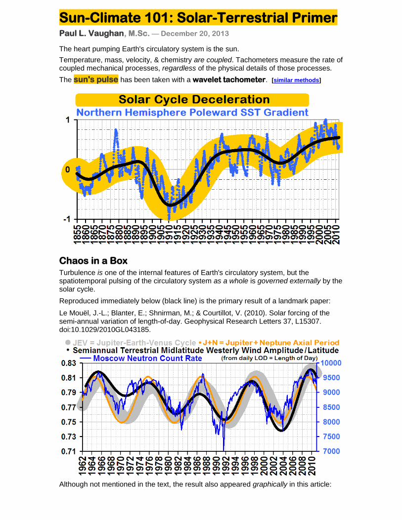
Sun-Climate 101: Solar-Terrestrial Primer

Paul L. Vaughan, M.Sc. — December 20, 2013

The heart pumping Earth's circulatory system is the sun.

Temperature, mass, velocity, & chemistry are coupled. Tachometers measure the rate of coupled mechanical processes, regardless of the physical details of those processes.

The sun's pulse has been taken with a wavelet tachometer. [similar methods]

Chaos in a Box

Turbulence is one of the internal features of Earth's circulatory system, but the spatiotemporal pulsing of the circulatory system as a whole is governed externally by the solar cycle.

Reproduced immediately below (black line) is the primary result of a landmark paper:

Le Mouël, J.-L.; Blanter, E.; Shnirman, M.; & Courtillot, V. (2010). Solar forcing of the semi-annual variation of length-of-day. Geophysical Research Letters 37, L15307. doi:10.1029/2010GL043185.

Although not mentioned in the text, the result also appeared graphically in this article:

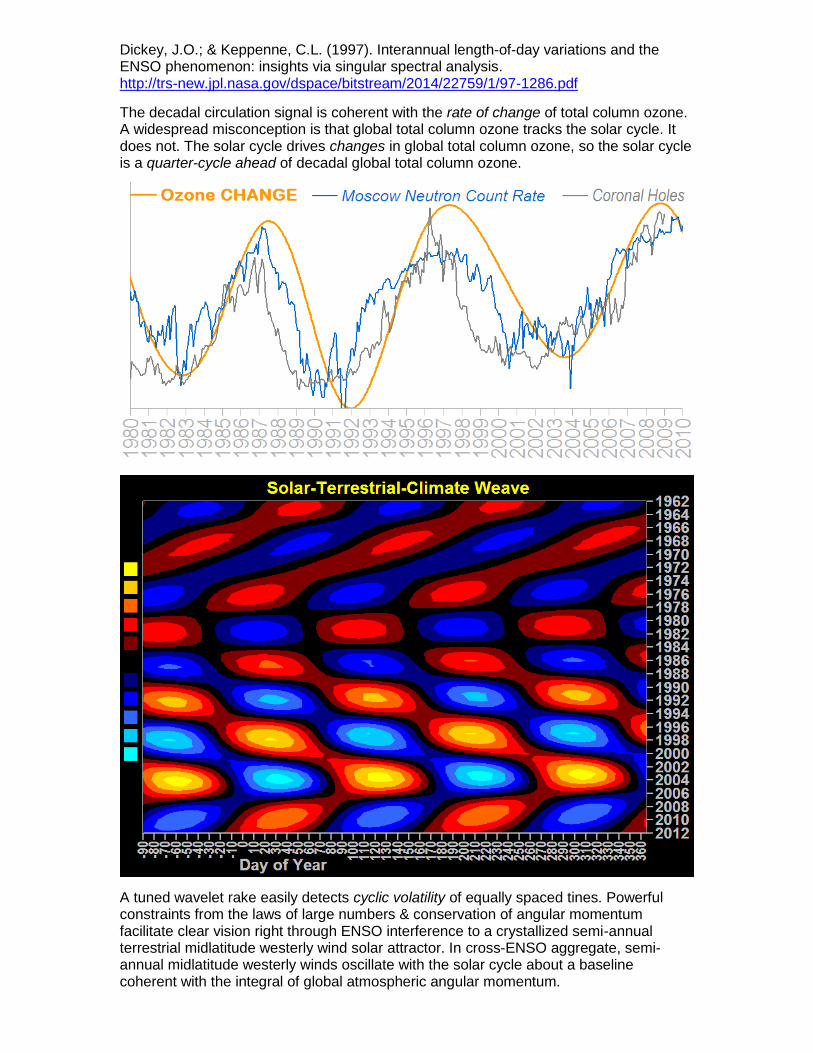
Dickey, J.O.; & Keppenne, C.L. (1997). Interannual length-of-day variations and the ENSO phenomenon: insights via singular spectral analysis. http://trs-new.jpl.nasa.gov/dspace/bitstream/2014/22759/1/97-1286.pdf

The decadal circulation signal is coherent with the rate of change of total column ozone. A widespread misconception is that global total column ozone tracks the solar cycle. It does not. The solar cycle drives changes in global total column ozone, so the solar cycle is a quarter-cycle ahead of decadal global total column ozone.

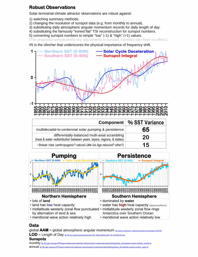
A tuned wavelet rake easily detects cyclic volatility of equally spaced tines. Powerful constraints from the laws of large numbers & conservation of angular momentum facilitate clear vision right through ENSO interference to a crystallized semi-annual terrestrial midlatitude westerly wind solar attractor. In cross-ENSO aggregate, semi-annual midlatitude westerly winds oscillate with the solar cycle about a baseline coherent with the integral of global atmospheric angular momentum.

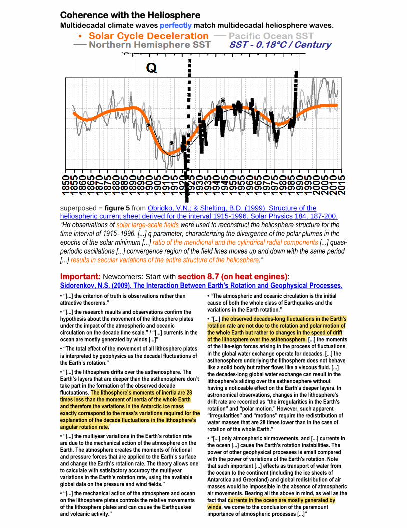
Robust Observations

Solar-terrestrial-climate attractor observations are robust against:

1) switching summary methods. 2) changing the resolution of sunspot data (e.g. from monthly to annual). 3) substituting daily atmospheric angular momentum records for daily length of day. 4) substituting the famously "ironed flat" TSI reconstruction for sunspot numbers. 5) converting sunspot numbers to simple "low" (-1) & "high" (+1) values. (The proposed comparatively tiny adjustments to sunspot numbers also have no effect.)

#5 is the clincher that underscores the physical importance of frequency shift.

Component % SST Variance multidecadal-to-centennial solar pumping & persistence 65

differentially-balanced multi-axial scrambling (heat & water redistribution between years, layers, regions, & states) 20 ~linear rise (anthropogenic? natural Little Ice Age rebound? other?) 15

Pumping Persistence

Northern Hemisphere Southern Hemisphere

• lots of land • land has low heat capacity • midlatitude westerly zonal flow punctuated

by alternation of land & sea • meridional wave action relatively high

• dominated by water • water has high heat capacity (delayed equilibrium) • midlatitude westerly zonal flow rings

Antarctica over Southern Ocean • meridional wave action relatively low

Data global AAM = global atmospheric angular momentum http://ftp.aer.com/pub/anon_collaborations/sba/aam.ncep.reanalysis.1948.2009

LOD = Length of Day ftp://ftp.iers.org/products/eop/long-term/c04_08/iau2000/eopc04_08_IAU2000.62-now

Sunspots monthly ftp://ftp.ngdc.noaa.gov/STP/space-weather/solar-data/solar-indices/sunspot-numbers/international/listings/listing_international-sunspot-numbers_monthly.txt annual ftp://ftp.ngdc.noaa.gov/STP/space-weather/solar-data/solar-indices/sunspot-numbers/international/listings/listing_international-sunspot-numbers_yearly.txt

Coherence with the Heliosphere

Multidecadal climate waves perfectly match multidecadal heliosphere waves.

superposed = figure 5 from Obridko, V.N.; & Shelting, B.D. (1999). Structure of the heliospheric current sheet derived for the interval 1915-1996. Solar Physics 184, 187-200.

“Hα observations of solar large-scale fields were used to reconstruct the heliosphere structure for the time interval of 1915–1996. [...] q parameter, characterizing the divergence of the polar plumes in the epochs of the solar minimum [...] ratio of the meridional and the cylindrical radial components [...] quasi-periodic oscillations [...] convergence region of the field lines moves up and down with the same period [...] results in secular variations of the entire structure of the heliosphere.”

Important: Newcomers: Start with section 8.7 (on heat engines): Sidorenkov, N.S. (2009). The Interaction Between Earth's Rotation and Geophysical Processes.

• “[...] the criterion of truth is observations rather than attractive theorems.”

• “[...] the research results and observations confirm the hypothesis about the movement of the lithosphere plates under the impact of the atmospheric and oceanic circulation on the decade time scale.” / “[...] currents in the ocean are mostly generated by winds [...]”

• “The total effect of the movement of all lithosphere plates is interpreted by geophysics as the decadal fluctuations of the Earth’s rotation.”

• “[...] the lithosphere drifts over the asthenosphere. The Earth’s layers that are deeper than the asthenosphere don’t take part in the formation of the observed decade fluctuations. The lithosphere’s moments of inertia are 28 times less than the moment of inertia of the whole Earth and therefore the variations in the Antarctic ice mass exactly correspond to the mass’s variations required for the explanation of the decade fluctuations in the lithosphere’s angular rotation rate.”

• “[...] the multiyear variations in the Earth’s rotation rate are due to the mechanical action of the atmosphere on the Earth. The atmosphere creates the moments of frictional and pressure forces that are applied to the Earth’s surface and change the Earth’s rotation rate. The theory allows one to calculate with satisfactory accuracy the multiyear variations in the Earth’s rotation rate, using the available global data on the pressure and wind fields.”

• “[...] the mechanical action of the atmosphere and ocean on the lithosphere plates controls the relative movements of the lithosphere plates and can cause the Earthquakes and volcanic activity.”

• “The atmospheric and oceanic circulation is the initial cause of both the whole class of Earthquakes and the variations in the Earth rotation.”

• “[...] the observed decades-long fluctuations in the Earth's rotation rate are not due to the rotation and polar motion of the whole Earth but rather to changes in the speed of drift of the lithosphere over the asthenosphere. [...] the moments of the like-sign forces arising in the process of fluctuations in the global water exchange operate for decades. [...] the asthenosphere underlying the lithosphere does not behave like a solid body but rather flows like a viscous fluid. [...] the decades-long global water exchange can result in the lithosphere's sliding over the asthenosphere without having a noticeable effect on the Earth's deeper layers. In astronomical observations, changes in the lithosphere's drift rate are recorded as “the irregularities in the Earth's rotation” and “polar motion.” However, such apparent “irregularities” and “motions” require the redistribution of water masses that are 28 times lower than in the case of rotation of the whole Earth.”

• “[...] only atmospheric air movements, and [...] currents in the ocean [...] cause the Earth's rotation instabilities. The power of other geophysical processes is small compared with the power of variations of the Earth's rotation. Note that such important [...] effects as transport of water from the ocean to the continent (including the ice sheets of Antarctica and Greenland) and global redistribution of air masses would be impossible in the absence of atmospheric air movements. Bearing all the above in mind, as well as the fact that currents in the ocean are mostly generated by winds, we come to the conclusion of the paramount importance of atmospheric processes [...]”

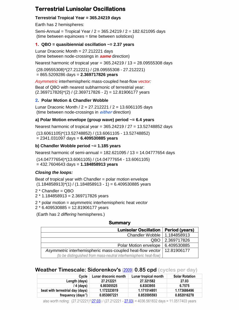
Terrestrial Lunisolar Oscillations

Terrestrial Tropical Year = 365.24219 days

Earth has 2 hemispheres:

Semi-Annual = Tropical Year / 2 = 365.24219 / 2 = 182.621095 days (time between equinoxes = time between solstices)

1. QBO = quasibiennial oscillation ~= 2.37 years

Lunar Draconic Month = 27.212221 days (time between node-crossings in same direction)

Nearest harmonic of tropical year = 365.24219 / 13 = 28.09555308 days

(28.09555308)*(27.212221) / (28.09555308 - 27.212221) = 865.5209286 days = 2.369717826 years

Asymmetric interhemispheric mass-coupled heat-flow vector:

Beat of QBO with nearest subharmonic of terrestrial year: (2.369717826)*(2) / (2.369717826 - 2) = 12.81906177 years

2. Polar Motion & Chandler Wobble

Lunar Draconic Month / 2 = 27.212221 / 2 = 13.6061105 days (time between node-crossings in either direction)

a) Polar Motion envelope (group wave) period ~= 6.4 years

Nearest harmonic of tropical year = 365.24219 / 27 = 13.52748852 days

(13.6061105)*(13.52748852) / (13.6061105 - 13.52748852) = 2341.031097 days = 6.409530885 years

b) Chandler Wobble period ~= 1.185 years

Nearest harmonic of semi-annual = 182.621095 / 13 = 14.04777654 days

(14.04777654)*(13.6061105) / (14.04777654 - 13.6061105) = 432.7604643 days = 1.184858913 years

Closing the loops:

Beat of tropical year with Chandler = polar motion envelope (1.184858913)*(1) / (1.184858913 - 1) = 6.409530885 years

2 * Chandler = QBO 2 * 1.184858913 = 2.369717826 years

2 * polar motion = asymmetric interhemispheric heat vector 2 * 6.409530885 = 12.81906177 years

(Earth has 2 differing hemispheres.)

Summary

Lunisolar Oscillation Period (years)

Chandler Wobble 1.184858913

QBO 2.369717826

Polar Motion envelope 6.409530885

Asymmetric interhemispheric mass-coupled heat-flow vector (to be distinguished from mass-neutral interhemispheric heat-flow)

12.81906177

Weather Timescale: Sidorenkov's (2009) 0.85 cpd (cycles per day)

Cycle Lunar draconic month Lunar tropical month Solar Rotation

Length (days) 27.212221 27.321582 27.03

/ 4 (days) 6.80305525 6.8303955 6.7575

beat with terrestrial day (days) 1.172323019 1.171514951 1.173686496

frequency (days-1) 0.853007221 0.853595593 0.852016278

also worth noting: (27.212221)*(27.03) / (27.212221 - 27.03) = 4036.561832 days = 11.0517403 years

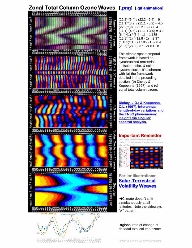
Zonal Total Column Ozone Waves [.png] [.gif animation]

(22.2)*(6.4) / (22.2 - 6.4) = 9 (11.1)*(3.2) / (11.1 - 3.2) = 4.5 (22.2)*(9) / (22.2 + 9) = 6.4 (11.1)*(4.5) / (11.1 + 4.5) = 3.2 (6.4)*(1) / (6.4 - 1) = 1.185 (12.8)*(2) / (12.8 - 2) = 2.37 (1.185)*(1) / (1.185 - 1) = 6.4 (2.37)*(2) / (2.37 - 2) = 12.8 This simple spatiotemporal framework is based on synchronized terrestrial, lunisolar, solar, & solar system clocks. It's coherent with (a) the framework detailed in the preceding section, (b) Dickey & Keppenne (1997), and (c) zonal total column ozone.

Dickey, J.O.; & Keppenne, C.L. (1997). Interannual length-of-day variations and the ENSO phenomenon: insights via singular spectral analysis.

Important Reminder (we only need a few more years of data to draw some hard conclusions about this...)

_______________________

Earlier Illustrations:

Solar-Terrestrial Volatility Weaves

◄Climate doesn't shift simultaneously at all latitudes. Note the sideways "w" pattern.

◄global rate of change of decadal total column ozone

Ozone is a sensitive climate indicator.

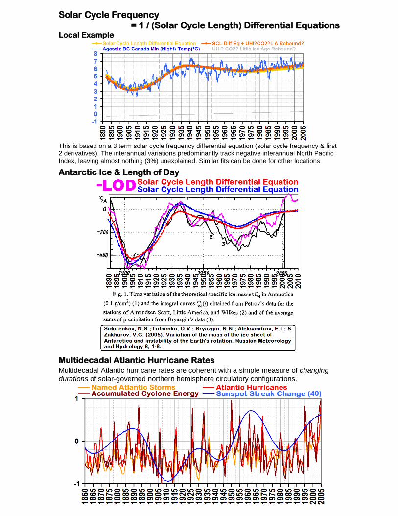
Solar Cycle Frequency = 1 / (Solar Cycle Length) Differential Equations

Local Example

This is based on a 3 term solar cycle frequency differential equation (solar cycle frequency & first 2 derivatives). The interannual variations predominantly track negative interannual North Pacific Index, leaving almost nothing (3%) unexplained. Similar fits can be done for other locations.

Antarctic Ice & Length of Day

Multidecadal Atlantic Hurricane Rates

Multidecadal Atlantic hurricane rates are coherent with a simple measure of changing durations of solar-governed northern hemisphere circulatory configurations.

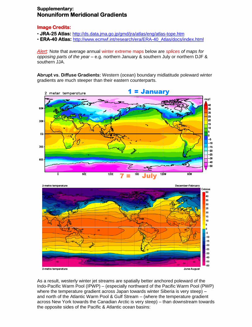
Supplementary:

Nonuniform Meridional Gradients Image Credits:

• JRA-25 Atlas: http://ds.data.jma.go.jp/gmd/jra/atlas/eng/atlas-tope.htm

• ERA-40 Atlas: http://www.ecmwf.int/research/era/ERA-40_Atlas/docs/index.html

Alert: Note that average annual winter extreme maps below are splices of maps for opposing parts of the year – e.g. northern January & southern July or northern DJF & southern JJA.

Abrupt vs. Diffuse Gradients: Western (ocean) boundary midlatitude poleward winter gradients are much steeper than their eastern counterparts.

As a result, westerly winter jet streams are spatially better anchored poleward of the Indo-Pacific Warm Pool (IPWP) – (especially northward of the Pacific Warm Pool (PWP) where the temperature gradient across Japan towards winter Siberia is very steep) – and north of the Atlantic Warm Pool & Gulf Stream – (where the temperature gradient across New York towards the Canadian Arctic is very steep) – than downstream towards the opposite sides of the Pacific & Atlantic ocean basins:

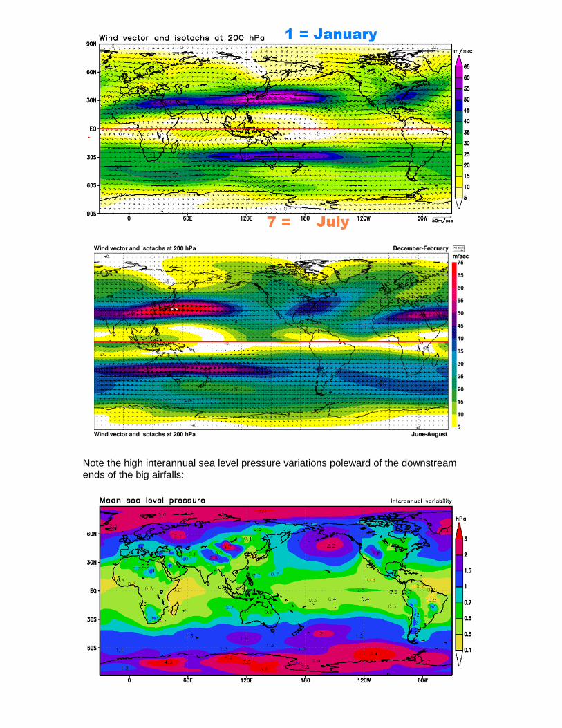
Note the high interannual sea level pressure variations poleward of the downstream ends of the big airfalls:

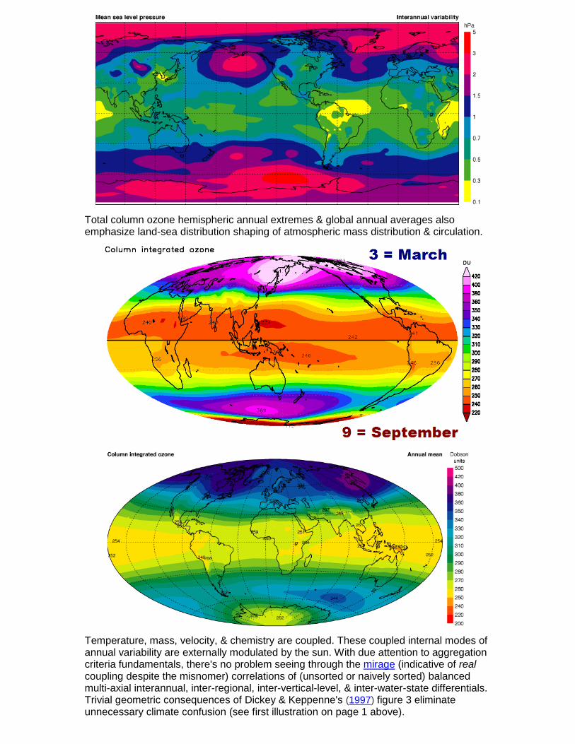
Total column ozone hemispheric annual extremes & global annual averages also emphasize land-sea distribution shaping of atmospheric mass distribution & circulation.

Temperature, mass, velocity, & chemistry are coupled. These coupled internal modes of annual variability are externally modulated by the sun. With due attention to aggregation criteria fundamentals, there's no problem seeing through the mirage (indicative of real coupling despite the misnomer) correlations of (unsorted or naively sorted) balanced multi-axial interannual, inter-regional, inter-vertical-level, & inter-water-state differentials. Trivial geometric consequences of Dickey & Keppenne's (1997) figure 3 eliminate unnecessary climate confusion (see first illustration on page 1 above).

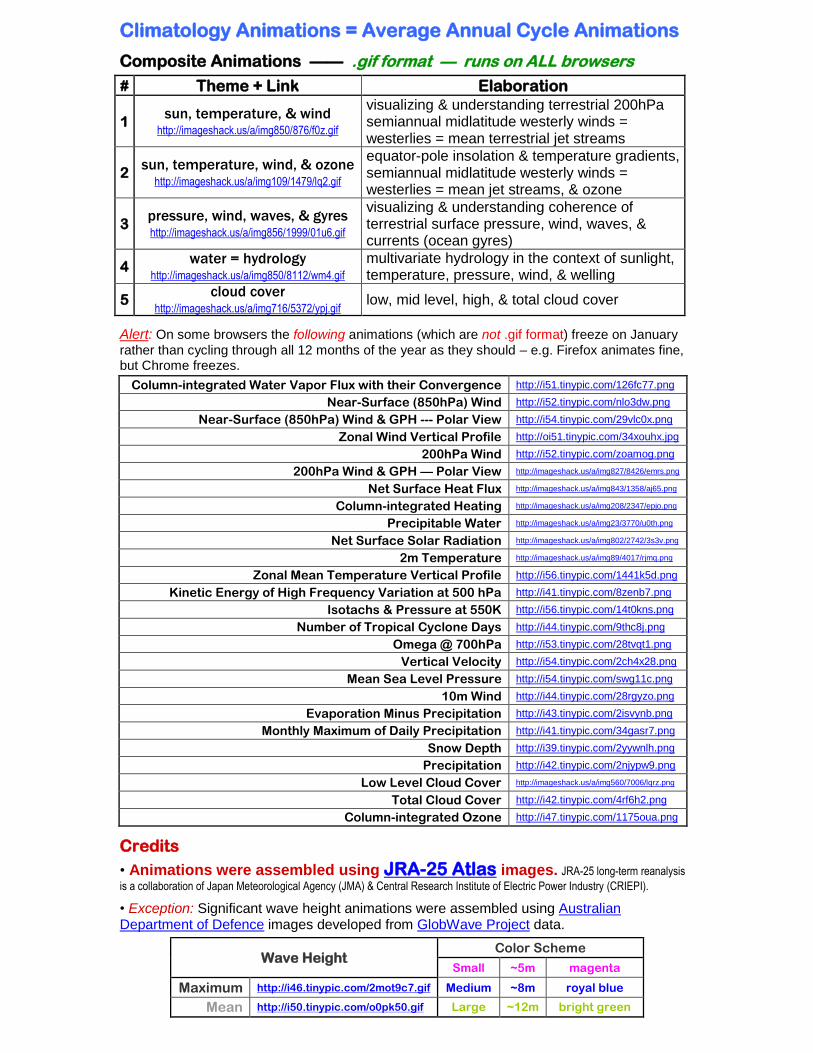
Climatology Animations = Average Annual Cycle Animations

Composite Animations —— .gif format — runs on ALL browsers

# Theme + Link Elaboration

1 sun, temperature, & wind

http://imageshack.us/a/img850/876/f0z.gif

visualizing & understanding terrestrial 200hPa semiannual midlatitude westerly winds = westerlies = mean terrestrial jet streams

2 sun, temperature, wind, & ozone

http://imageshack.us/a/img109/1479/lq2.gif

equator-pole insolation & temperature gradients, semiannual midlatitude westerly winds = westerlies = mean jet streams, & ozone

3 pressure, wind, waves, & gyres http://imageshack.us/a/img856/1999/01u6.gif

visualizing & understanding coherence of terrestrial surface pressure, wind, waves, & currents (ocean gyres)

4 water = hydrology

http://imageshack.us/a/img850/8112/wm4.gif

multivariate hydrology in the context of sunlight, temperature, pressure, wind, & welling

5 cloud cover

http://imageshack.us/a/img716/5372/ypj.gif low, mid level, high, & total cloud cover

Alert: On some browsers the following animations (which are not .gif format) freeze on January

rather than cycling through all 12 months of the year as they should – e.g. Firefox animates fine, but Chrome freezes.

Column-integrated Water Vapor Flux with their Convergence http://i51.tinypic.com/126fc77.png

Near-Surface (850hPa) Wind http://i52.tinypic.com/nlo3dw.png

Near-Surface (850hPa) Wind & GPH --- Polar View http://i54.tinypic.com/29vlc0x.png

Zonal Wind Vertical Profile http://oi51.tinypic.com/34xouhx.jpg

200hPa Wind http://i52.tinypic.com/zoamog.png

200hPa Wind & GPH — Polar View http://imageshack.us/a/img827/8426/emrs.png

Net Surface Heat Flux http://imageshack.us/a/img843/1358/aj65.png

Column-integrated Heating http://imageshack.us/a/img208/2347/epjo.png

Precipitable Water http://imageshack.us/a/img23/3770/u0th.png

Net Surface Solar Radiation http://imageshack.us/a/img802/2742/3s3v.png

2m Temperature http://imageshack.us/a/img89/4017/rjmq.png

Zonal Mean Temperature Vertical Profile http://i56.tinypic.com/1441k5d.png

Kinetic Energy of High Frequency Variation at 500 hPa http://i41.tinypic.com/8zenb7.png

Isotachs & Pressure at 550K http://i56.tinypic.com/14t0kns.png

Number of Tropical Cyclone Days http://i44.tinypic.com/9thc8j.png

Omega @ 700hPa http://i53.tinypic.com/28tvqt1.png

Vertical Velocity http://i54.tinypic.com/2ch4x28.png

Mean Sea Level Pressure http://i54.tinypic.com/swg11c.png

10m Wind http://i44.tinypic.com/28rgyzo.png

Evaporation Minus Precipitation http://i43.tinypic.com/2isvynb.png

Monthly Maximum of Daily Precipitation http://i41.tinypic.com/34gasr7.png

Snow Depth http://i39.tinypic.com/2yywnlh.png

Precipitation http://i42.tinypic.com/2njypw9.png

Low Level Cloud Cover http://imageshack.us/a/img560/7006/lqrz.png

Total Cloud Cover http://i42.tinypic.com/4rf6h2.png

Column-integrated Ozone http://i47.tinypic.com/1175oua.png

Credits

• Animations were assembled using JRA-25 Atlas images. JRA-25 long-term reanalysis

is a collaboration of Japan Meteorological Agency (JMA) & Central Research Institute of Electric Power Industry (CRIEPI).

• Exception: Significant wave height animations were assembled using Australian Department of Defence images developed from GlobWave Project data.

Wave Height Color Scheme

Small ~5m magenta

Maximum http://i46.tinypic.com/2mot9c7.gif Medium ~8m royal blue

Mean http://i50.tinypic.com/o0pk50.gif Large ~12m bright green

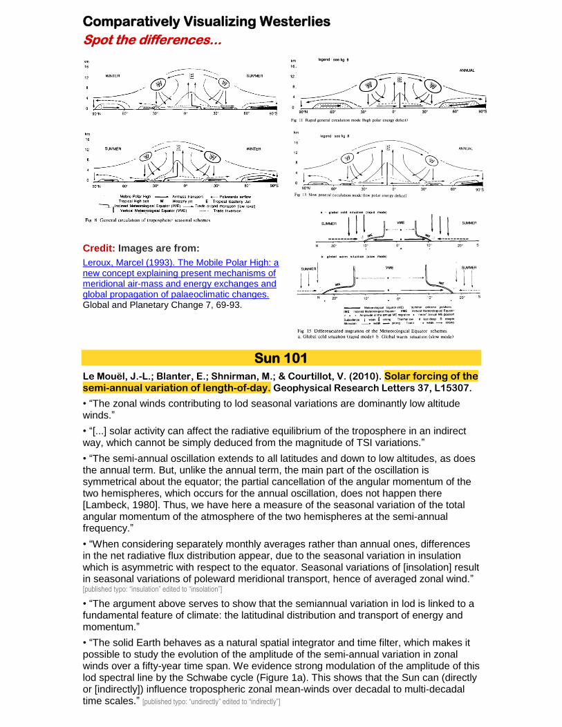
Comparatively Visualizing Westerlies

Spot the differences...

Credit: Images are from:

Leroux, Marcel (1993). The Mobile Polar High: a new concept explaining present mechanisms of meridional air-mass and energy exchanges and global propagation of palaeoclimatic changes. Global and Planetary Change 7, 69-93.

Sun 101

Le Mouël, J.-L.; Blanter, E.; Shnirman, M.; & Courtillot, V. (2010). Solar forcing of the semi-annual variation of length-of-day. Geophysical Research Letters 37, L15307.

• “The zonal winds contributing to lod seasonal variations are dominantly low altitude winds.”

• “[...] solar activity can affect the radiative equilibrium of the troposphere in an indirect way, which cannot be simply deduced from the magnitude of TSI variations.”

• “The semi-annual oscillation extends to all latitudes and down to low altitudes, as does the annual term. But, unlike the annual term, the main part of the oscillation is symmetrical about the equator; the partial cancellation of the angular momentum of the two hemispheres, which occurs for the annual oscillation, does not happen there [Lambeck, 1980]. Thus, we have here a measure of the seasonal variation of the total angular momentum of the atmosphere of the two hemispheres at the semi-annual frequency.”

• “When considering separately monthly averages rather than annual ones, differences in the net radiative flux distribution appear, due to the seasonal variation in insulation which is asymmetric with respect to the equator. Seasonal variations of [insolation] result in seasonal variations of poleward meridional transport, hence of averaged zonal wind.” [published typo: “insulation” edited to “insolation”]

• “The argument above serves to show that the semiannual variation in lod is linked to a fundamental feature of climate: the latitudinal distribution and transport of energy and momentum.”

• “The solid Earth behaves as a natural spatial integrator and time filter, which makes it possible to study the evolution of the amplitude of the semi-annual variation in zonal winds over a fifty-year time span. We evidence strong modulation of the amplitude of this lod spectral line by the Schwabe cycle (Figure 1a). This shows that the Sun can (directly or [indirectly]) influence tropospheric zonal mean-winds over decadal to multi-decadal time scales.” [published typo: “undirectly” edited to “indirectly”]

Foundations

“Apart from all other reasons, the parameters of the geoid depend on the distribution of water over the planetary surface.” – Nikolay Sidorenkov

• Concise overview of heat engines = p.433 [pdf p.10] here:

Sidorenkov, N.S. (2005). Physics of the Earth’s rotation instabilities. Astronomical and Astrophysical Transactions 24(5), 425-439.

• For more on heat engines, see section 8.7 here:

Sidorenkov, N.S. (2009). The Interaction Between Earth's Rotation and Geophysical Processes. Wiley.

They got it wrong...

“There are three possible sources for the 65-70-yr 'global' oscillation: (1) random forcing, such as by white noise; (2) external oscillatory forcing, such as by a variation in the solar constant; and (3) an internal oscillation of the atmosphere-ocean system. Atmospheric white-noise forcing of the ocean, evoking a red-noise response, was proposed by Hasselmann [22] and has been invoked to explain the non-GHG+ASA component of the observed temperature record [12]. Putative variations in the solar constant have also been proposed to explain this [23,24,10]. But it is unlikely that either of these forcings is the source of the 65-70-yr oscillation—solar forcing should generate a global response [25,26] and white-noise forcing an ocean-wide response, but the 65-70-yr oscillation is neither global nor pan-oceanic. The most probable cause of this oscillation is therefore an internal oscillation of the atmospheric-ocean system.” [GHG = greenhouse-gas; ASA = anthropogenic sulphate-aerosol]

Schlesinger, M.E.; & Ramankutty, N. (1994). An oscillation in the global climate system. Nature 367, 723-726.

...but it can be fixed:

Challenge for Climate Modelers

Sensibly adapt to overcome Sidorenkov's (2009) simplification (p.184 [pdf p.198]):

“[...] hereafter we will neglect the variations in W [...]”

When due care is taken to view clustered volatility through a bifocal lens balanced to avoid nonlinear ENSO water redistribution bias, equator-to-polar-night spatial gradients are seen to vary in lockstep with the solar cycle as illustrated by Dickey & Keppenne (NASA JPL 1997 Figure 3b) and clarified by Le Mouël, Blanter, Shnirman, & Courtillot (Solar forcing of the semi-annual variation of length-of-day [2010]).

The geometric consequences are simple – (see pages 1-3 above). These insights are governed by the laws of large numbers & conservation of angular momentum.

Climate evolution isn't only a function of total energy input, but also the spatiotemporal gradient of input, the driver of mixing. Wind's the primary driver of ocean currents, welling, evaporation, ice transport, & solar-paced stirring more generally.

Supplementary Reading

Gross, R.S. (2007). Earth rotation variations – long period. In: Herring, T.A. (ed.), Treatise on Geophysics vol. 11 (Physical Geodesy), Elsevier, Amsterdam.

Schmitz-Hubsch, H.; & Schuh, H. (1999). Seasonal and short-period fluctuations of Earth rotation investigated by wavelet analysis. Technical Report 1999.6-2 Department of Geodesy & Geoinformatics, Stuttgart University, p.421-432.