Summer School on Multidimensional Poverty

8–19 July 2013

Institute for International Economic Policy (IIEP) George Washington University

Washington, DC

Regression Analysis with AF measures

Paola Ballón Oxford Poverty & Human Development

Initiative (OPHI)

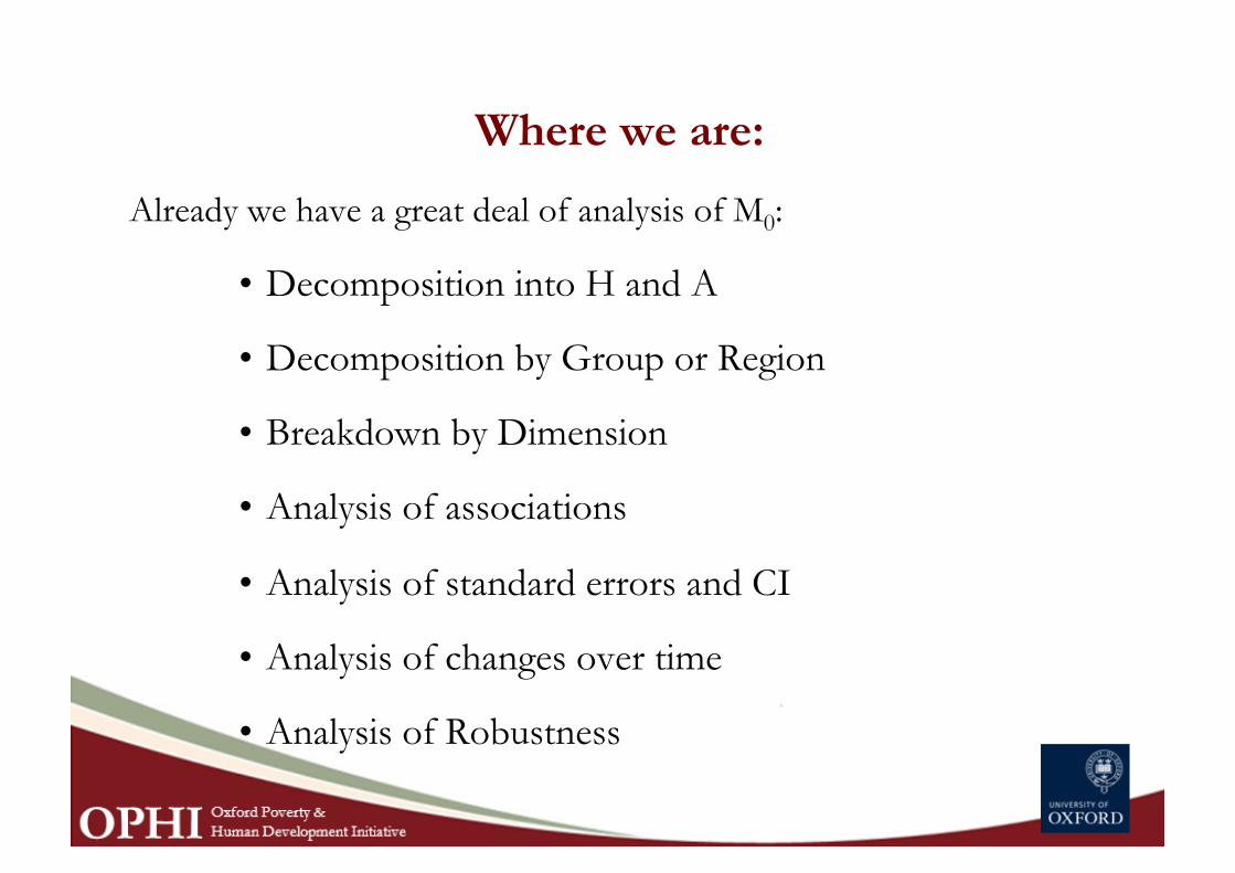
Where we are:

Already we have a great deal of analysis of M0:

• Decomposition into H and A

• Decomposition by Group or Region

•  Breakdown by Dimension

• Analysis of associations

• Analysis of standard errors and CI

• Analysis of changes over time

• Analysis of Robustness

What are we missing?

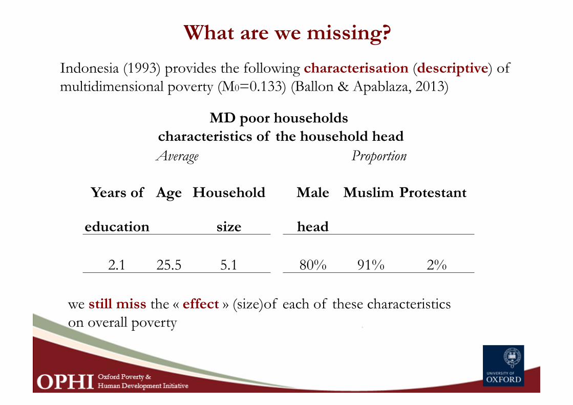
Indonesia (1993) provides the following characterisation (descriptive) of multidimensional poverty (M0=0.133) (Ballon & Apablaza, 2013)

MD poor households characteristics of the household head Average Proportion

Years of Age Household Male Muslim Protestant

education size head

2.1 25.5 5.1 80% 91% 2%

we still miss the « effect » (size)of each of these characteristics on overall poverty

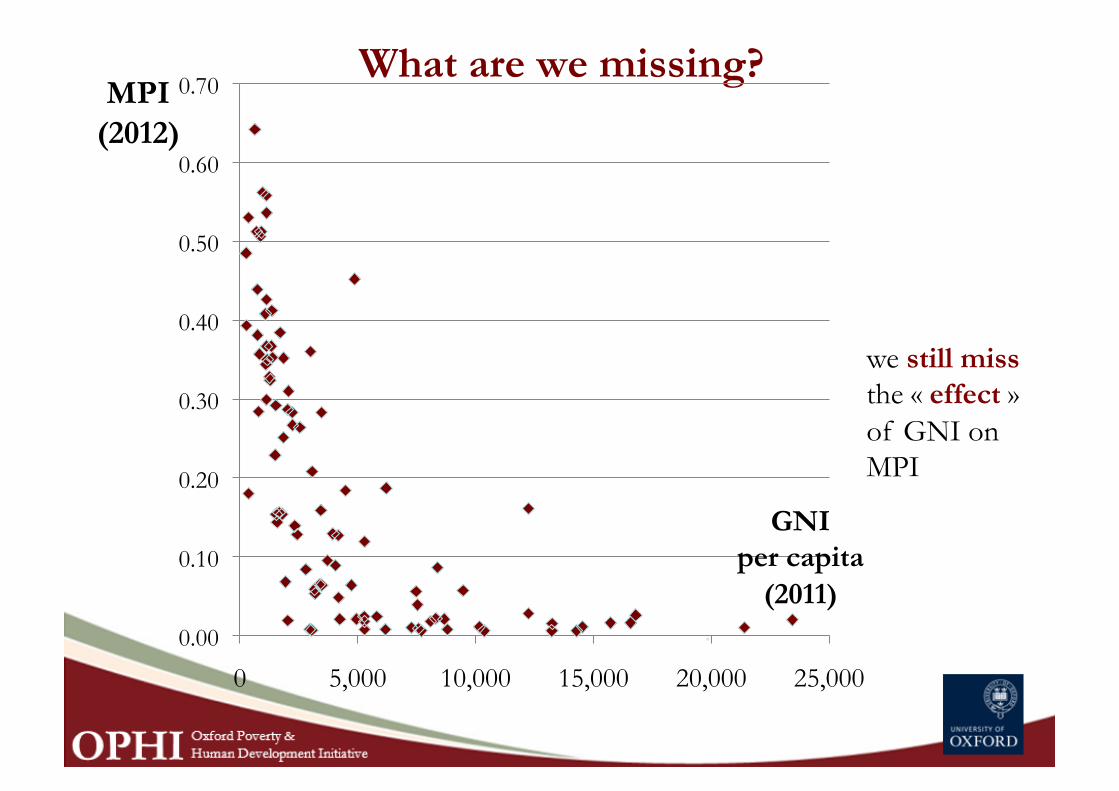
What are we missing?

we still miss the « effect » of GNI on MPI

0.00

0.10

0.20

0.30

0.40

0.50

0.60

0.70

0 5,000 10,000 15,000 20,000 25,000

MPI (2012)

GNI per capita

(2011)

Why is this important?

From a policy angle, it is useful to understand the transmission mechanisms of macro policies and poverty measures.

This is to assess how poverty is explained by non-Mα related variables

How can we account for this?

Through Regression Analysis we can account for the “effect/size” of micro and macro determinants of multidimensional poverty.

This allows for an analysis of interactions with variables not used for obtaining M0

We can differentiate between:

a) ‘micro’ regressions: unit of analysis is the household or the person

b) ‘macro’ regressions: unit analysis is some “spatial” aggregate, such as a province, a district or a country.

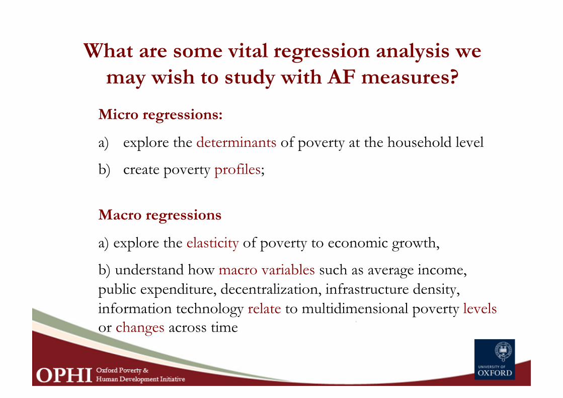
What are some vital regression analysis we may wish to study with AF measures?

Micro regressions:

a)  explore the determinants of poverty at the household level

b)  create poverty profiles;

Macro regressions

a) explore the elasticity of poverty to economic growth,

b) understand how macro variables such as average income, public expenditure, decentralization, infrastructure density, information technology relate to multidimensional poverty levels or changes across time

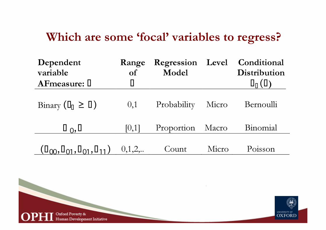
Which are some ‘focal’ variables to regress?

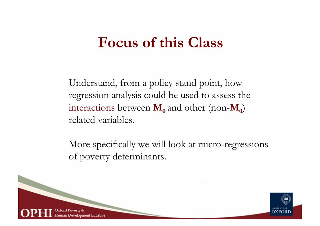
Focus of this Class

Understand, from a policy stand point, how regression analysis could be used to assess the interactions between M0 and other (non-M0) related variables.

More specifically we will look at micro-regressions of poverty determinants.

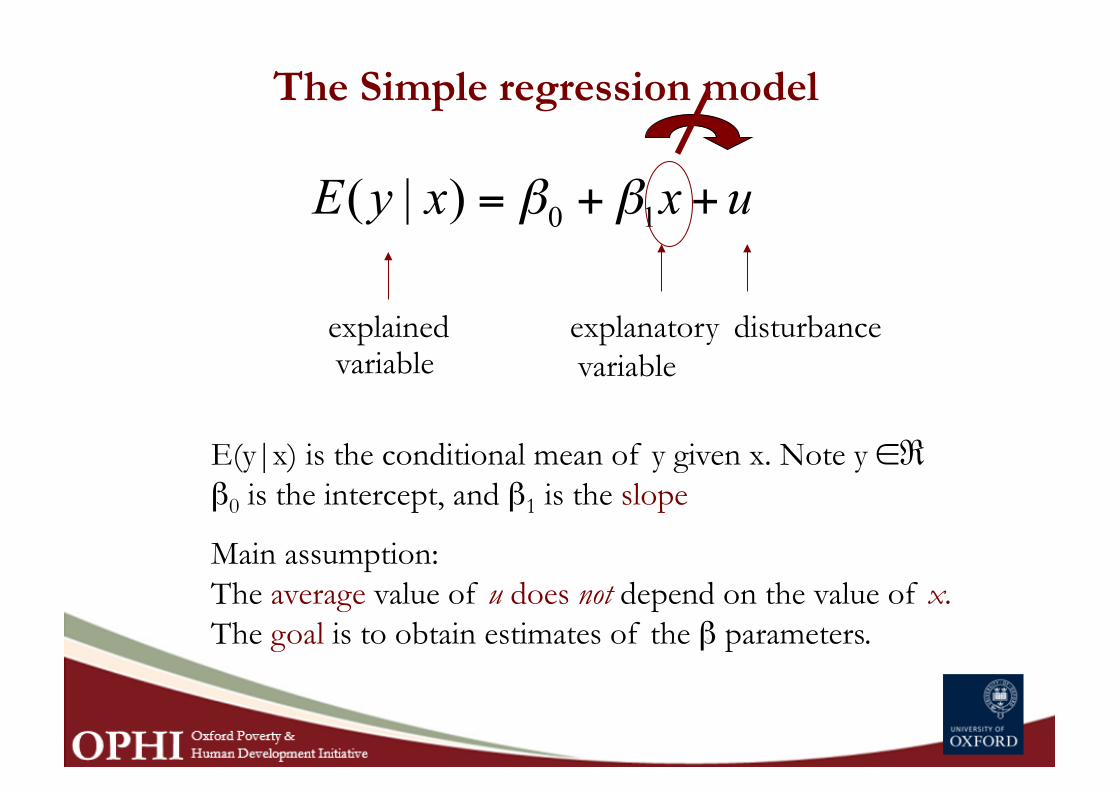
The Simple regression model

explanatory explained disturbance variable variable

E(y|x) is the conditional mean of y given x. Note y ∈ℜ β0 is the intercept, and β1 is the slope

Main assumption: The average value of u does not depend on the value of x. The goal is to obtain estimates of the β parameters.

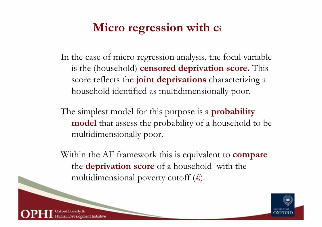
Micro regression with ci

In the case of micro regression analysis, the focal variable is the (household) censored deprivation score. This score reflects the joint deprivations characterizing a household identified as multidimensionally poor.

The simplest model for this purpose is a probability model that assess the probability of a household to be multidimensionally poor.

Within the AF framework this is equivalent to compare the deprivation score of a household with the multidimensional poverty cutoff (k).

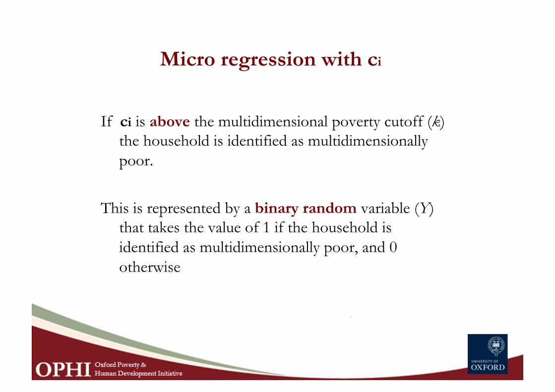
Micro regression with ci

If ci is above the multidimensional poverty cutoff (k) the household is identified as multidimensionally poor.

This is represented by a binary random variable (Y) that takes the value of 1 if the household is identified as multidimensionally poor, and 0 otherwise

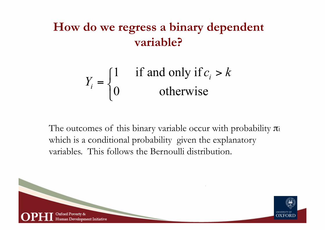
How do we regress a binary dependent variable?

The outcomes of this binary variable occur with probability πi which is a conditional probability given the explanatory variables. This follows the Bernoulli distribution.

Probit and Logit models The simple linear regression model is not adequate as it assumes that the range of the dependent variable lies in the Real line (-∞, +∞)

To ensure that the conditional mean stays in the unit interval we need some function that maps Y to the unit interval.

Any cumulative distribution function could be used for this purpose.

Often the cumulative distributions of the standard normal distribution or the logistic distribution are used to model binary responses. This leads to what is called as probit or logit models respectively.

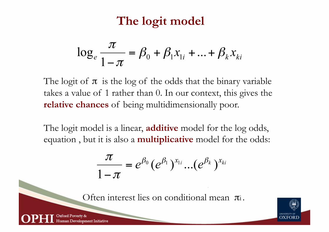
The logit model

The logit of π is the log of the odds that the binary variable takes a value of 1 rather than 0. In our context, this gives the relative chances of being multidimensionally poor.

The logit model is a linear, additive model for the log odds, equation , but it is also a multiplicative model for the odds:

Often interest lies on conditional mean πi .

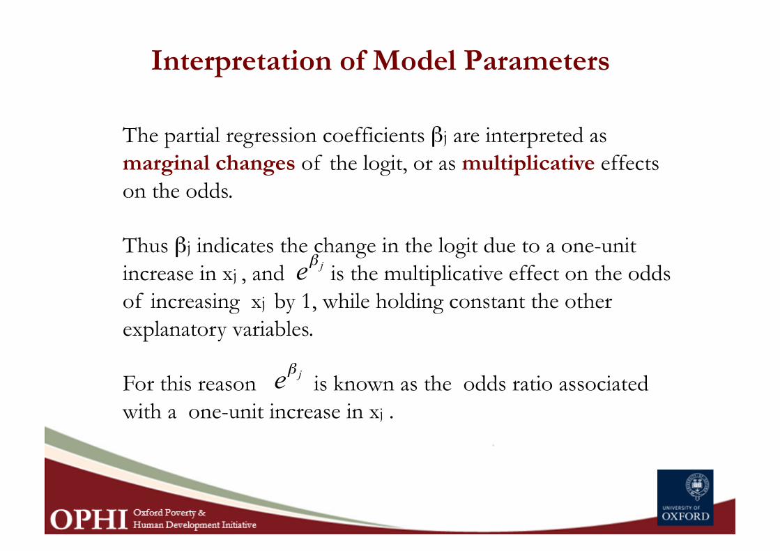
Interpretation of Model Parameters

The partial regression coefficients βj are interpreted as marginal changes of the logit, or as multiplicative effects on the odds.

Thus βj indicates the change in the logit due to a one-unit increase in xj , and is the multiplicative effect on the odds of increasing xj by 1, while holding constant the other explanatory variables.

For this reason is known as the odds ratio associated with a one-unit increase in xj .

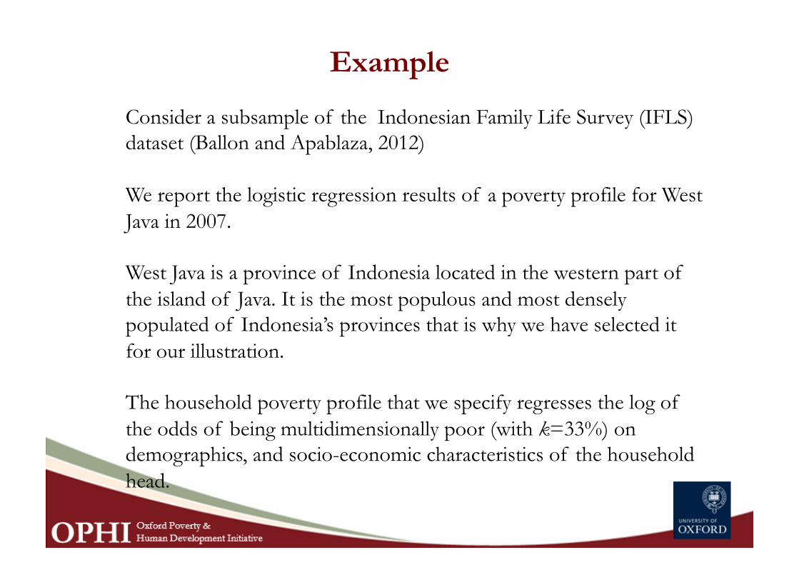
Example

Consider a subsample of the Indonesian Family Life Survey (IFLS) dataset (Ballon and Apablaza, 2012)

We report the logistic regression results of a poverty profile for West Java in 2007.

West Java is a province of Indonesia located in the western part of the island of Java. It is the most populous and most densely populated of Indonesia’s provinces that is why we have selected it for our illustration.

The household poverty profile that we specify regresses the log of the odds of being multidimensionally poor (with k=33%) on demographics, and socio-economic characteristics of the household head.

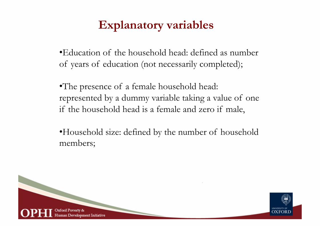
Explanatory variables

• Education of the household head: defined as number of years of education (not necessarily completed);

• The presence of a female household head: represented by a dummy variable taking a value of one if the household head is a female and zero if male,

• Household size: defined by the number of household members;

Explanatory variables

• The area in which the household resides: represented by a dummy variable taking a value of one if the household resides in urban areas of West Java and zero otherwise;

• Muslim religion: represented by a dummy variable taking a value of one if the household’s main religion is Muslim, and zero if not.

These have been selected on the grounds of ‘restraining’ any ‘possible’ endogeneity  issue that may arise in the construction of a household multidimensional poverty profile.

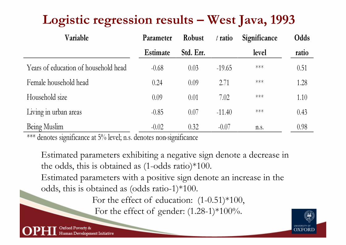
Logistic regression results – West Java, 1993

Estimated parameters exhibiting a negative sign denote a decrease in the odds, this is obtained as (1-odds ratio)*100. Estimated parameters with a positive sign denote an increase in the odds, this is obtained as (odds ratio-1)*100.

For the effect of education: (1-0.51)*100, For the effect of gender: (1.28-1)*100%.

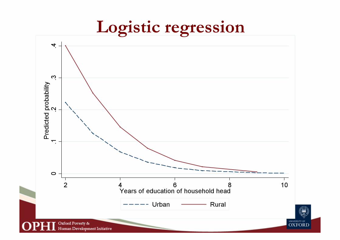
Logistic regression

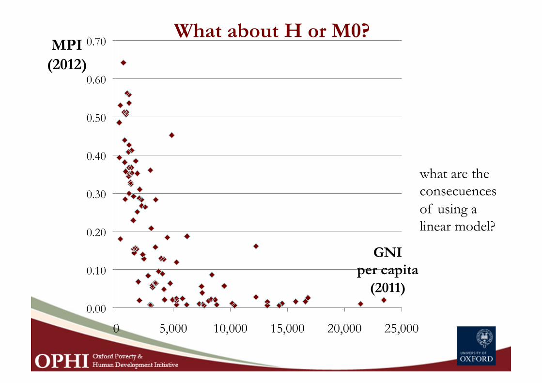
What about H or M0?

what are the consecuences of using a linear model?

0.00

0.10

0.20

0.30

0.40

0.50

0.60

0.70

0 5,000 10,000 15,000 20,000 25,000

MPI (2012)

GNI per capita

(2011)

What about H, M0?

H and M0 are indices, bounded between zero and one

Thus an econometric model for these endogenous variables must account for the shape of their distribution, which has a restricted range of variation that lies in the unit interval.,

H and M0 are therefore fractional (proportion) variables bounded between zero and one with the possibility of observing values at the boundaries.

Can we specify a simple linear regression for

H and M0? Specifying a linear model assumes that the endogenous variable and its mean take any value in the real line.

This is not adequate for fractional thus specifying a linear model and estimating it ordinary least squares is not the right strategy, as this ignores the shape of the distribution of these dependent variables.

If the interest of the research question is not in modeling the conditional mean of the proportion but rather in modeling the absolute change (between two time periods), that can take any value, standard linear regression models apply. 

Approaches to Model a Proportion We can differentiate between one and two-part approaches. These differ in the treatment of the boundary values of the fractional dependent variable.

In a one-step approach one considers a single model for the entire distribution of the values of the proportion; where both the limiting observations and those falling inside the unit interval are modeled together.

In a two-step approach the observations at the boundaries are modeled separately from those falling inside the unit interval. (Wagner, 2001; Ramalho and Ramalho, 2011).

The decision whether a one or a two-part model is appropriate is often based on theoretical economic arguments (Ballon, 2013).

Four one-step approaches

The first of them simply ignores the bounded nature of the proportion and assume a linear conditional mean. It is clear that this approach is unreasonable because a linear specification cannot guarantee that the predicted or fitted values of the fraction will not be outside the unit interval.

An alternative approach is to use a log-transformation of the proportion after adding an arbitrarily chosen small constant to all observations. Clearly this transformation modifies the distribution of the dependent variable in an ad hoc manner and thus it is not appropriate.

Four one-step approaches The third approach is to apply Tobit models for data that is censored at 1 and/or 0. This approach has also some drawbacks. As pointed out by Maddala (1991), Tobit models are appropriate for modeling censored data; this is data where the zeros or/and ones are censored by definition. Tobit models are conceptually inappropriate when the boundary observations are a natural consequence of the theoretical mechanism characterizing the data, which is our case.

The fourth approach is to assume a particular conditional distribution for the proportion like the Beta distribution. The Beta distribution is a continuous distribution defined only in the open interval (0,1) and thus the probability of observing a certain value, like the boundaries, is zero (Wagner, 2001; Ramalho and Ramalho, 2011) .

Papke and Wooldridge approach

To model H or M0 we follow the modeling approach proposed by Papke and Wooldridge (1996).

Let’s denote the adjusted headcount ratio or the incidence of some spatial spatial aggregate, say a country, by yi

Papke and Wooldridge propose a particular quasi-likelihood method to estimate a proportion.

The method follows Gourieroux, Monfort and Trognon(1984) and McCullagh and Nelder (1989) and is based on the Bernoulli log-likelihood function

To summarize

We have considered a probit/logit model using ci

We have also seen that H and M0 requiere models for fractional data.

We can also consider other types of models.

We may be interested in studying the probability of been multidimensionally poor and monetary poor (bi-probit)

Or studying the dynamics over time.

Some references

Comparision of one vs. two part approaches : Ballon (2013)

Bi-probit: Chatterjee, M. (2013)

Macro determinants of H and M0 in Indonesia: Ballon and Apablaza(2013)

Thank you