Summed Score Likelihood–

Article

Educational and PsychologicalMeasurement

1–30� The Author(s) 2017

Reprints and permissions:sagepub.com/journalsPermissions.nav

DOI: 10.1177/0013164417717024journals.sagepub.com/home/epm

Summed Score Likelihood–Based Indices for TestingLatent Variable DistributionFit in Item Response Theory

Zhen Li1 and Li Cai2

Abstract

In standard item response theory (IRT) applications, the latent variable is typicallyassumed to be normally distributed. If the normality assumption is violated, the itemparameter estimates can become biased. Summed score likelihood–based statisticsmay be useful for testing latent variable distribution fit. We develop Satorra–Bentlertype moment adjustments to approximate the test statistics’ tail-area probability. Asimulation study was conducted to examine the calibration and power of the unad-justed and adjusted statistics in various simulation conditions. Results show that theproposed indices have tail-area probabilities that can be closely approximated by cen-tral chi-squared random variables under the null hypothesis. Furthermore, the teststatistics are focused. They are powerful for detecting latent variable distributionalassumption violations, and not sensitive (correctly) to other forms of model misspeci-fication such as multidimensionality. As a comparison, the goodness-of-fit statistic M2

has considerably lower power against latent variable nonnormality than the proposedindices. Empirical data from a patient-reported health outcomes study are used asillustration.

Keywords

item response theory, goodness of fit, normality

1eMetric, San Antonio, TX, USA2University of California, Los Angeles, CA, USA

Corresponding Author:

Li Cai, CRESST, 300 Charles E. Young Drive North, GSEIS building, University of California, Los Angeles,

CA 90095-1522, USA.

Email: [email protected]

https://doi.dox.org/10.1177/0013164417717024

Introduction

Item response theory (IRT) provides powerful methods supporting educational and

psychological measurement (Thissen & Steinberg, 2009). The latent variable in IRT

models is usually assumed to follow a normal distribution for the purpose of item

parameter estimation (Bock & Aitkin, 1981; Bock & Lieberman, 1970). However,

this assumption might be violated in some situations (Woods, 2006; Woods & Lin,

2009). Woods (2006) described several potential situations where u may be nonnor-

mal. For example, as severe symptoms of psychological disorders rarely exist in the

general population and most people have low levels of psychopathological symp-

toms, latent variables reflecting these symptoms may be positively skewed. Another

possible cause arises in the situation when the population is heterogeneous. For

instance, when two or more subpopulations with different means and variances are

grouped together, potentially multimodal population distributions may be the result.

Calibrating the items with respect to the combined population renders the normality

assumption suspect. When the assumption of normal latent variable distribution is

violated, the item parameter estimates might be biased, leading to bias in subsequent

inferences based on these item parameter estimates. Take computer adaptive testing

as an example, the item parameter estimates are used for both item selection and test

scoring. Thus, bias in the estimation of item parameters might result in significant

bias in the reported test scores.

Although alternative approaches exist for estimating the latent variable distribu-

tion in standard IRT models (Bock & Aitkin, 1981; Woods & Lin, 2009; Woods &

Thissen, 2006), these approaches are computationally more demanding and specia-

lized software is necessary. For example, in our experience, the empirical histogram

representation of the latent prior distribution is often less stable numerically than the

standard normal prior. Thus, it is worthwhile to test the assumption of latent variable

normality before more ‘‘expensive’’ approaches are applied. Summed score

likelihood–based statistics may be useful for testing latent variable distribution fit.

One problem is that the statistics do not asymptotically follow a chi-squared distribu-

tion. We propose a Satorra–Bentler type moment adjustment method (Satorra &

Bentler, 1994) in this article. The statistics’ tail-area probability can be approximated

by making use of the item parameter error covariance matrix and a Jacobian. The

properties of the adjusted and unadjusted statistics are examined by simulation and

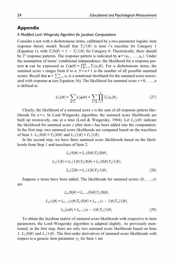
empirical studies. Additionally, a modified Lord–Wingersky algorithm for comput-

ing the Jacobian matrix is presented in the appendix.

Item Response Theory Models

In standard IRT models, the conditional item response probabilities (also referred to

as item tracelines or item characteristic curves) are represented as a function of latent

variable u and item parameters. For example, the three-parameter logistic (3PL)

model can be written as

2 Educational and Psychological Measurement

Ti 1juð Þ= gi +1� gi

1 + exp � ci + aiuð Þ½ � , ð1Þ

where Ti 1juð Þ represents item i’s traceline for the 1 category (indicating correct/

endorsement response in most contexts) as a function of u. The item parameters

include: gi, which is the pseudoguessing probability for the item (the lower asymptote

parameter); ai, which is the slope (the discrimination parameter), and ci, which is the

item intercept parameter. The classical difficulty (threshold) parameter is obtained

as�ci=ai. If gi is 0, the model reduces to a two-parameter logistic (2PL) model, and if

all the item slopes are constrained to be equal to a common slope (ai[a), the one-

parameter logistic (1PL) model is the result. The incorrect/nonendorsement response

probability is equal toTi 0juð Þ = 1� Ti 1juð Þ.For an item with Ki ordered polytomous responses, the graded response model is

often used. Let the response categories be coded as k = 0, . . . Ki � 1. The cumulative

response probability for item i in categories k and above is

T+i kjuð Þ = 1

1 + exp � cik + aiuð Þ½ � , ð2Þ

for k = 1, . . . Ki � 1. Having defined the boundary cases T+i 0juð Þ = 1 and

T+i Kijuð Þ = 0, the category response probabilities can be written as

Ti kjuð Þ= T+i kjuð Þ � T+

i k + 1juð Þ, ð3Þ

for k = 0, . . . Ki � 1. Let Ui be a random variable whose realization ui is a response

to item i. Regardless of the number of categories, the probability mass function of Ui,

conditional on u, is that of a multinomial with trial size 1:

P Ui = uijuð Þ =YKi�1

k = 0

Ti uijuð Þ½ �1k uið Þ, ð4Þ

where 1k uið Þ is an indicator function such that

1k uið Þ=1, if k = ui

0, otherwise

�: ð5Þ

The Latent Variable Distribution in IRT

Estimating the latent variable distribution along with item parameters using the

empirical histogram (Bock & Aitkin, 1981; Mislevy, 1984; Zimowski, Muraki,

Mislevy, & Bock, 1996) is an established strategy for detecting and correcting latent

variable nonnormality in IRT. Newer semiparametric density estimation procedures

offer more efficient alternatives. These include the Ramsay Curve IRT (Woods &

Thissen, 2006), and Davidian Curve IRT (Monroe & Cai, 2014; Woods & Lin,

2009), as well as its multidimensional extension (Monroe, 2014). In practice,

Li and Cai 3

however, estimating latent variable densities often requires specialized software.

More complex latent variable distributions also involve more parameters to be esti-

mated from the data, increasing the need for larger calibration sample sizes to

achieve stable estimation. Finally, even as nonnormal latent densities may be mod-

eled, for example, using a Ramsay curve IRT model (Woods & Thissen, 2006), and

the relative model fit may be evaluated against a baseline using likelihood ratio tests,

it does not circumvent the need for absolute goodness-of-fit indices to establish the

adequacy of the least restrictive model in the class of models being compared (see

Maydeu-Olivares & Cai, 2006, for further explanation). It would be highly desirable

to establish a set of statistics that can be used to diagnose the extent to which a nor-

mal (or nonnormal) latent variable distribution may in fact be a reasonable characteri-

zation before more ‘‘expensive’’ methods and software programs for semiparametric

density estimation are used.

In developing such a group of test statistics for latent variable distribution fit, sev-

eral desiderata should be taken into account. First, the statistics should be easily com-

putable, preferably using only standard by-products of the item calibration process.

Second, the statistics should have well-grounded heuristic motivation and theoretical

justification. Third, the frequency calibration of the statistics under the null hypoth-

esis should be sufficiently accurate. Finally, the statistics should have adequate power

that is focused on latent variable distribution assumption violation and sufficient diag-

nostic specificity, rather than becoming a surrogate of overall model fit tests.

The guiding insight has been provided elsewhere in the literature. For unidimen-

sional IRT modeling, the observed and model-implied summed score distribution can

be a basis for inferring the adequacy of the latent variable distribution specification

in the IRT model (Thissen & Wainer, 2001). After model fitting, residual summed

score probabilities may be used to construct chi-square test statistics. While the idea

itself is not new (see, Ferrando & Lorenzo-seva, 2001; Hambleton & Traub, 1973;

Lord, 1953; Ross, 1966; Sinharay, Johnson, & Stern, 2006, among others), we use

the recently developed theory of limited-information goodness-of-fit testing to for-

mally demonstrate that the summed score likelihood–based fit index proposed here

belongs to the general family of multinomial limited-information tests.

The Multinomial Sampling Model and Maximum LikelihoodEstimation

Let there be I items in a test. Under the conditional independence assumption, the

IRT model specifies the conditional response pattern probability as the following

product:

P \I

i = 1Ui = uiju

� �=YI

i = 1

P Ui = uijuð Þ: ð6Þ


Assuming that g uð Þ is the distribution of the latent variable (also known as the

prior distribution), the marginal response pattern probability is the following integral:

P \I

i = 1Ui = ui

� �=

ðYI

i = 1

P Ui = uijuð Þg uð Þdu = pu gð Þ, ð7Þ

where u = u1, . . . , uIð Þ is the response pattern, and g is a d31 vector that collects

together the free item parameters from all I items. The parenthetical notation pu gð Þin Equation (7) is used to emphasize the fact that it is the model. The marginal

response probability depends on the item parameters, the item-level response models,

and the assumed latent variable distribution.

Recall that Ki is the number of categories for item i. For I items, the IRT model

generates a total of C =QI

i = 1 Ki cross-classifications or possible item response pat-

terns in the form of a contingency table. Based on a sample of N respondents, let the

observed proportion associated with pattern u be denoted as pu. The sampling model

for this contingency table is a multinomial distribution with C cells and N trials. The

multinomial log-likelihood for the item parameters g is proportional to

log L gð Þ}NX

u

pu log pu gð Þ, ð8Þ

where the summation is over all C response patterns. Maximization of the log-

likelihood (e.g., with the expectation–maximization algorithm; Bock & Aitkin, 1981)

leads to the maximum marginal likelihood estimator g.

On finding g, the IRT model generates model-implied probabilities for each

response pattern pu gð Þ = pu. Suppose the model-implied response pattern probabil-

ities pu are collected into a C31 vector p of all model-implied response pattern prob-

abilities. By analogy, let a C31 vector p contain the true (population) response

pattern probabilities. Similarly, the observed proportions pu can be collected into a

C31 vector p. For example, for three dichotomously scored items there are 23 = 8

item response patterns, and the response pattern probabilities and observed propor-

tions are

p =

p000

p001

p010

p011

p100

p101

p110

p111

0BBBBBBBBB@

1CCCCCCCCCA

, p =

p000

p001

p010

p011

p100

p101

p110

p111

0BBBBBBBBB@

1CCCCCCCCCA

=

p000 gð Þp001 gð Þp010 gð Þp011 gð Þp100 gð Þp101 gð Þp110 gð Þp111 gð Þ

0BBBBBBBBB@

1CCCCCCCCCA

, p =

p000

p001

p010

p011

p100

p101

p110

p111

0BBBBBBBBB@

1CCCCCCCCCA: ð9Þ

From results in discrete multivariate analysis (e.g., Bishop, Fienberg, & Holland,

1975), g is consistent, asymptotically normal, and asymptotically efficient, which

can be summarized as follows:

Li and Cai 5

ffiffiffiffiNp

g � gð Þ!D N d 0,F�1� �

, ð10Þ

where F = D0 diag pð Þ½ ��1D is the d3d Fisher information matrix, with the Jacobian

matrix D defined as the C3d matrix of all first-order partial derivatives of the

response patterns probabilities with respect to the item parameters:

D =∂p gð Þ∂g0

: ð11Þ

Distribution of Residuals Under Maximum LikelihoodEstimation

Based on Equation (10), it can be shown that the asymptotic distribution of the differ-

ence p� pð Þ is C-variate normal:

ffiffiffiffiNp

p� pð Þ!D N C 0, Nð Þ, ð12Þ

where N = diag pð Þ � pp0 is the covariance matrix associated with the multinomial.

The residual vector p� pð Þ is asymptotically C-variate normal under maximum like-

lihood estimation:

ffiffiffiffiNp

p� pð Þ!D N C 0, Gð Þ, ð13Þ

where G = N� DF�1D0, and the second term reflects variability due to estimation of

item parameters.

Lower Order Marginal Probabilities

The IRT model implies marginal probabilities. Consider the three-item example from

above. There are three first-order marginal probabilities _pi i = 1, . . . , 3ð Þ, one per

item. There are also three second-order marginal probabilities €pij for the unique item

pairs (1 � j\i � 3). In general, these probabilities correspond to the I univariate and

I I � 1ð Þ=2 bivariate margins that can be obtained from the full C-dimensional con-

tingency table using a reduction operator matrix (see e.g., Maydeu-Olivares & Joe,

2005). An example is given below:

p2 ¼

_p1

_p2

_p3

€p21

€p31

€p32

0BBBBBB@

1CCCCCCA¼ Lp ¼

0 0 0 0 1 1 1 1

0 0 1 1 0 0 1 1

0 1 0 1 0 1 0 1

0 0 0 0 0 0 1 1

0 0 0 0 0 1 0 1

0 0 0 1 0 0 0 1

0BBBBBB@

1CCCCCCA

p000

p001

p010

p011

p100

p101

p110

p111

0BBBBBBBBBB@

1CCCCCCCCCCA

ð14Þ


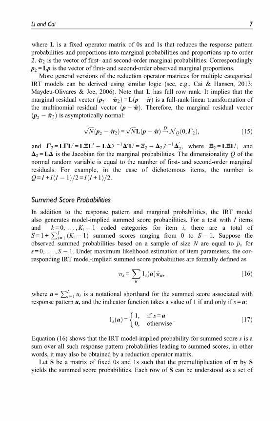
where L is a fixed operator matrix of 0s and 1s that reduces the response pattern

probabilities and proportions into marginal probabilities and proportions up to order

2. p2 is the vector of first- and second-order marginal probabilities. Correspondingly

p2 = Lp is the vector of first- and second-order observed marginal proportions.

More general versions of the reduction operator matrices for multiple categorical

IRT models can be derived using similar logic (see, e.g., Cai & Hansen, 2013;

Maydeu-Olivares & Joe, 2006). Note that L has full row rank. It implies that the

marginal residual vector p2 � p2ð Þ = L p� pð Þ is a full-rank linear transformation of

the multinomial residual vector p� pð Þ. Therefore, the marginal residual vector

p2 � p2ð Þ is asymptotically normal:

ffiffiffiffiNp

p2 � p2ð Þ =ffiffiffiffiNp

L p� pð Þ!D N Q 0, G2ð Þ, ð15Þ

and G2 = LGL0 = LNL0 � LDF�1D0L0 = N2 � D2F�1D0

2, where N2 = LNL0, and

D2 = LD is the Jacobian for the marginal probabilities. The dimensionality Q of the

normal random variable is equal to the number of first- and second-order marginal

residuals. For example, in the case of dichotomous items, the number is

Q = I + I I � 1ð Þ=2 = I I + 1ð Þ=2.

Summed Score Probabilities

In addition to the response pattern and marginal probabilities, the IRT model

also generates model-implied summed score probabilities. For a test with I items

and k = 0, . . . , Ki � 1 coded categories for item i, there are a total of

S = 1 +PI

i = 1 Ki � 1ð Þ summed scores ranging from 0 to S � 1. Suppose the

observed summed probabilities based on a sample of size N are equal to �ps for

s = 0, . . . , S � 1. Under maximum likelihood estimation of item parameters, the cor-

responding IRT model-implied summed score probabilities are formally defined as

�ps =X

u

1s uð Þpu, ð16Þ

where u =PI

i = 1 ui is a notational shorthand for the summed score associated with

response pattern u, and the indicator function takes a value of 1 if and only if s = u:

1s uð Þ= 1, if s = u

0, otherwise

�: ð17Þ

Equation (16) shows that the IRT model-implied probability for summed score s is a

sum over all such response pattern probabilities leading to summed scores, in other

words, it may also be obtained by a reduction operator matrix.

Let S be a matrix of fixed 0s and 1s such that the premultiplication of p by S

yields the summed score probabilities. Each row of S can be understood as a set of

Li and Cai 7

binary logical relations. An element in row j of S is equal to 1 if and only if the corre-

sponding response pattern in p leads to summed score j� 1. In general, for I items,

there are S rows and C columns in S. In particular, S has full row rank and the rows

of S are mutually orthogonal.

Returning to the three-item example, there are four summed scores in this case: 0,

1, 2, and 3. The 438 matrix S (below) relates the summed score probabilities to the

original multinomial probabilities:

�p =

�p0

�p1

�p2

�p3

0B@

1CA= Sp =

1 0

0 1

0 0

1 00 0

0 0

0 1

0 0

0 0

1 0

0 0

0 00 1

0 0

1 0

0 1

0B@

1CA

p000

p001

p010

p011

p100

p101

p110

p111

0BBBBBBBBB@

1CCCCCCCCCA

,

�p =

�p0

�p1

�p2

�p3

0BB@

1CCA= Sp: ð18Þ

The observed summed score proportions can be obtained in a similar way:

�p =

�p0

�p1

�p2

�p3

0B@

1CA= Sp =

1 0

0 1

0 0

1 00 0

0 0

0 1

0 0

0 0

1 0

0 0

0 00 1

0 0

1 0

0 1

0B@

1CA

p000

p001

p010

p011

p100

p101

p110

p111

0BBBBBBBBB@

1CCCCCCCCCA: ð19Þ

From Equation (13), under maximum likelihood estimation, the summed score

residual vector �p� �p is asymptotically S-variate normally distributed:

ffiffiffiffiNp

�p� �p� �

=ffiffiffiffiNp

Sp� Spð Þ=ffiffiffiffiNp

S p� pð Þ!D N S 0, Gð Þ, ð20Þ

and �G = SGS0 = Sdiag pð ÞS0 � Spp0S0 � SDF�1D0S0 = diag �pð Þ � �p�p0 � �DF�1 �D

0,

with �D = SD.

The reason for introducing the reduction operator matrix S is primarily a theoreti-

cal one. It facilitates the subsequent derivations of summed score likelihood–based

indices for testing latent variable distribution fit. Pragmatically, the Lord–Wingersky

(1984) algorithm should be used to compute the model-implied summed score prob-

abilities. If summed score to scale score conversion tables are computed (see, Thissen

& Wainer, 2001), the probabilities become automatic by-products.


Goodness-of-Fit Statistics for IRT models

Existing overall goodness-of-fit indices may be used for testing latent variable distri-

bution fit in IRT. The full-information test statistics such as likelihood ratio G2 and

Pearson’s X2 use residuals based on the full response pattern cross-classifications to

test the IRT model against the general multinomial alternative. The comparison

between pu and pu (on logarithmic or linear scales) leads to well-known goodness-

of-fit statistics such as the likelihood ratio G2 and Pearson’s X2:

G2 = 2NX

u

pu logpu

pu

, X 2 = NX

u

pu � puð Þ2

pu

: ð21Þ

Under the null hypothesis that the IRT model fits exactly, these two statistics have

the same asymptotic reference distribution, which is a central chi-square with degrees

of freedom (df) equal to C � 1� d (Bishop et al., 1975). For subsequent develop-

ment, it is instructive to rewrite Pearson’s statistic as a quadratic form in multinomial

residuals: X 2 = N p� pð Þ0

diag pð Þ½ ��1p� pð Þ:

Unfortunately, as the number of items increases, the number of response patterns

increases exponentially. For more than a dozen or so dichotomous items (or perhaps

a handful of polytomous items), the contingency table on which the multinomial is

defined becomes sparse for any realistic N. Consequently, the asymptotic chi-square

approximations for the full-information test statistics break down (see, e.g.,

Bartholomew & Tzamourani, 1999) and the utility of the full-information overall

goodness-of-fit indices for routine IRT applications becomes questionable.

Recently, limited-information overall fit statistics such as Maydeu-Olivares and

Joe’s (2005) M2 have been developed. Limited-information fit statistics use residuals

based on lower order (e.g., first and second order) margins of the contingency table.

These lower order margins are far better filled when compared with the sparse full

contingency table. There is growing awareness that limited-information tests can

maintain correct size and can be more powerful than the full-information tests (Cai,

Maydeu-Olivares, Coffman, & Thissen, 2006; Joe & Maydeu-Olivares, 2010).

Under the assumption that the number of first- and second-order margins is larger

than the number of free parameters (Q . d) and that D2 has full column rank (local

identification), M2 can be written as

M2 = N p2 � p2ð Þ0 ~D2

~D02N2~D2

h i�1~D02 p2 � p2ð Þ, ð22Þ

where ~D2 is a Q3 Q� dð Þ orthogonal complement of D2 such that ~D02D2 = 0. From

Equation (15), p2 � p2ð Þ is asymptotically normal with zero means and covariance

matrix N2 � D2F�1D02, which implies that the covariance matrix of ~D0

2 p2 � p2ð Þ is~D02N2

~D2. Thus, M2 is asymptotically chi-square distributed with Q� d degrees of

freedom. In the current simulation study, M2 will be used as a benchmark because of

its numerous desirable properties identified in the literature (see, e.g., Cai & Hansen,

Li and Cai 9

2013). Performance of the proposed latent variable distribution fit indices will be

evaluated against M2.

While an overall test may be used to detect specification errors of latent variable

distributions, the fact that they are also sensitive to other forms of model error (e.g.,

unmodeled multidimensionality) makes it difficult to pinpoint the source of misspe-

cification. To that end, more specific diagnostic indices have been created for IRT.

For example, Chen and Thissen’s (1997) local dependence indices are particularly

sensitive to violations of the local independence assumption. Orlando and Thissen’s

(2000) item fit diagnostics is another example where the extent to which the IRT

model fits the empirical operating characteristics for an item (e.g., whether monoto-

nicity holds) can be examined. The next section develops a set of indices that specifi-

cally target latent variable distribution fit for IRT models.

The Summed Score Likelihood–Based Indices and StatisticalAdjustments

There are two important lines of reasoning for the derivation of these model fit

indices. The first is a recognition based on heuristics: IRT model–implied summed

score probabilities may provide useful diagnostic information about the latent vari-

able distributional assumption (Thissen & Wainer, 2001). The second recognition is

that the summed score likelihood–based indices are formally limited-information test

statistics.

A Heuristic Motivation

When the latent variable distribution assumed in the IRT model does not represent

the population distribution of the respondents adequately, the model-implied summed

score probabilities �ps will depart from the observed summed score probabilities �ps.

Hence all that is needed is to find appropriate test statistics that can summarize the

degree to which the model-implied and observed summed score probabilities diverge.

It is also preferable if the indices are approximately chi-square distributed test statis-

tics. Pearson’s X2 introduced in the previous section meets this requirement.

Recall that the total number of summed scores is S = 1 +PI

i = 1 Ki � 1ð Þ. The

Pearson-type �X 2 below yields a direct comparison between the model-implied

summed score probabilities �ps and the observed summed score probabilities �ps:

�X 2 = NXS�1

s = 0

�ps � �ps

� �2

�ps

, ð23Þ

where �ps and �ps represent the observed and model-implied summed score probability

for score s, respectively. This test statistic is different from the full-information test

statistic shown in Equation (21) because it is based on summed score probabilities as

opposed to response pattern probabilities.


In preliminary studies (Li & Cai, 2012) we had conjectured that under a wide

variety of conditions �X 2 may have similar asymptotic distributions whose tail-area

probabilities can be approximated by a central chi-squared random variable with

S � 1� 2 degrees of freedom under the null hypothesis that the latent variable distri-

bution g uð Þ is correctly specified in the IRT model. This conjecture will be tested in

the sequel with simulations.

The rationale behind the specific degrees of freedom is as follows: The S summed

scores’ probabilities must sum to 1. The first minus 1 is to reflect that constraint. Had

the item parameters been known, the degrees of freedom would have been exactly

S � 1. When the item parameters are estimated (assuming with maximum marginal

likelihood), an additional penalty must be introduced to reflect the effect of parameter

estimation. While the location and scale of the latent variable u are typically fixed for

model identification, the model-implied summed score distribution does not have an

inherent location and scale. The location and scale is determined as a result of estimat-

ing the item parameters. Hence, the estimation of item parameters amounts to adding at

least two more constraints for the model-implied summed score probability distribution.

The details are of course more complex, and will be explained next.

A More Formal Derivation

While the proposed test statistics are not associated with particular marginal prob-

abilities in the same manner as Maydeu-Olivares and Joe’s (2005) M2, they are nev-

ertheless related to the response pattern probabilities via the reduction operator

matrix S defined earlier (see Equations [18]). It is the choice of this particular reduc-

tion operator that leads to more focused tests targeting latent variable distribution fit

(see Joe & Maydeu-Olivares, 2010). For IRT models with constrained equal item

discrimination parameters (e.g., the 1PL model), it is widely recognized that the

summed scores are sufficient statistics for the latent variables in the model. Though

the summed score sufficiency property does not hold for other IRT models such as

the 2PL or the graded model, researchers have nevertheless found that summed score

is an important source of information regarding the ordering of individuals along the

latent variable continuum (e.g., van der Ark, 2005). One could even base parameter

estimation on summed score groups (Chen & Thissen, 1999).

Using the reduction operator S, the derivations above imply that the Pearson-type

statistic �X 2 can be rewritten as

�X 2 = NXS�1

s = 0

�ps � �ps

� �2

�ps

= N �p� �p� �0

diag �p� �� 1

�p� �p� �

, ð24Þ

where �p� �p� �

= S p� pð Þ is the summed score residual vector (see Equation [20]).

Under the null hypothesis that the IRT model is correctly specified, one can obtain

the probability limit of the weight matrix as plim diag �p� �� 1

�= diag �pð Þ½ ��1

by

Li and Cai 11

the consistency of the maximum likelihood estimator (see Equation 9), the continuity

of the mapping from g to the summed score probabilities, and the continuity of the

matrix inverse. Following results on quadratic forms of random vectors (e.g., Mathai

& Provost, 1992), the asymptotic expected value of �X 2 is equal to

tr �G diag �pð Þ½ ��1n o

= tr diag �pð Þ � �p�p0�

diag �pð Þ½ ��1n o

� tr �DF�1 �D0 diag �pð Þ½ ��1 �

= S � 1� tr F�1 �D0 diag �pð Þ½ ��1 �Dn o

= m1: ð25Þ

From Equations (24) and (25) we can see that the statistic �X 2 cannot be asymptoti-

cally chi-square distributed. Even though it is a quadratic form in asymptotically nor-

mally distributed random vectors, a key condition for its chi-squaredness is not met.

That is, the product of the probability limit of the weight matrix diag �pð Þ½ ��1and the

covariance matrix of the normal random vector �G is not idempotent in general, that

is, �G diag �pð Þ½ ��1 �G diag �pð Þ½ ��1 6¼ �G diag �pð Þ½ ��1. On the other hand, Equation (25)

shows that the asymptotic expected value of �X 2 is equal to S � 1 minus a constant

that depends on the trace of F�1 �D0 diag �pð Þ½ ��1 �D, which reflects additional uncer-

tainty due to estimation of item parameters. With the first-order moment of �X 2, the

Satorra–Bentler type moment adjustment approaches can be applied to adjust the sta-

tistic, so that the tail area of its distribution can be better approximated by a chi-

square distribution (Cai et al., 2006; Satorra & Bentler, 1994).

Adjustment of Statistics

According to Satorra and Bentler’s (1994) article, test statistics that do not asymptoti-

cally follow a chi-squared distribution can be corrected, by matching the mean (or the

mean & variance) to fixed degrees of freedom. Let df indicate the degrees of freedom

of interest, and m1 indicate the asymptotic expected value of �X 2. The moment-

adjusted statistic is

�X 2C = �X 2 m1

df

� ��1

: ð26Þ

Theoretically, the constant df can take on an arbitrary value. For the purpose of

comparison, df will take the value of S � 1� 2 in this article.

One challenge to obtain the adjusted statistics is calculating the first-order

moment in Equation (25). Some commercial software for IRT (e.g., flexMIRT�;

Cai, 2013) provides the Fisher information matrix F and the model-implied summed

score probabilities �p in the output file, but currently none of them produces the

Jacobian matrix �D. Numerical calculation of the Jacobian matrix can be computa-

tionally demanding, especially when the number of items (n) is large. Take the 2PL

IRT model as an example. It requires the computation of 232n first-order derivatives

to obtain �D. For a test of 12 items, 8,192 first-order derivatives need to be computed.

When n increases to 24, that requires 33,554,432 first-order derivatives to be


computed. To solve this problem, a modification of Lord–Wingersky algorithm

(Lord & Wingersky, 1984) for calculating the Jacobian matrix is developed (see the

appendix). Once the Jacobian matrix is computed, the first-order moments of �X 2 can

be computed.

Simulations

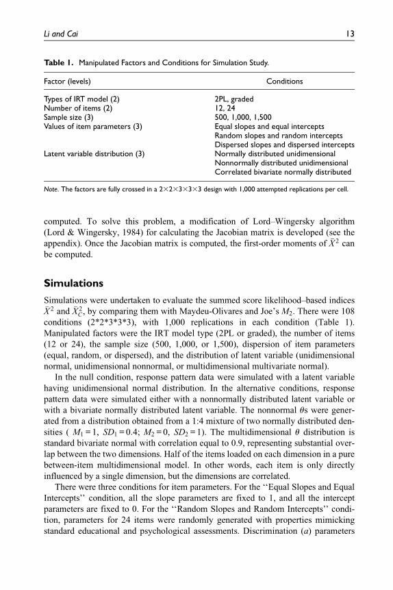
Simulations were undertaken to evaluate the summed score likelihood–based indices�X 2 and �X 2

C , by comparing them with Maydeu-Olivares and Joe’s M2. There were 108

conditions (2*2*3*3*3), with 1,000 replications in each condition (Table 1).

Manipulated factors were the IRT model type (2PL or graded), the number of items

(12 or 24), the sample size (500, 1,000, or 1,500), dispersion of item parameters

(equal, random, or dispersed), and the distribution of latent variable (unidimensional

normal, unidimensional nonnormal, or multidimensional multivariate normal).

In the null condition, response pattern data were simulated with a latent variable

having unidimensional normal distribution. In the alternative conditions, response

pattern data were simulated either with a nonnormally distributed latent variable or

with a bivariate normally distributed latent variable. The nonnormal us were gener-

ated from a distribution obtained from a 1:4 mixture of two normally distributed den-

sities ( M1 = 1, SD1 = 0:4; M2 = 0, SD2 = 1). The multidimensional u distribution is

standard bivariate normal with correlation equal to 0.9, representing substantial over-

lap between the two dimensions. Half of the items loaded on each dimension in a pure

between-item multidimensional model. In other words, each item is only directly

influenced by a single dimension, but the dimensions are correlated.

There were three conditions for item parameters. For the ‘‘Equal Slopes and Equal

Intercepts’’ condition, all the slope parameters are fixed to 1, and all the intercept

parameters are fixed to 0. For the ‘‘Random Slopes and Random Intercepts’’ condi-

tion, parameters for 24 items were randomly generated with properties mimicking

standard educational and psychological assessments. Discrimination (a) parameters

Table 1. Manipulated Factors and Conditions for Simulation Study.

Factor (levels) Conditions

Types of IRT model (2) 2PL, gradedNumber of items (2) 12, 24Sample size (3) 500, 1,000, 1,500Values of item parameters (3) Equal slopes and equal intercepts

Random slopes and random interceptsDispersed slopes and dispersed intercepts

Latent variable distribution (3) Normally distributed unidimensionalNonnormally distributed unidimensionalCorrelated bivariate normally distributed

Note. The factors are fully crossed in a 232333333 design with 1,000 attempted replications per cell.

Li and Cai 13

were drawn from a log-normal distribution M = 0:5, SD = 0:2ð Þ, the threshold values

(b) were drawn from a normal distribution M = 0, SD = 0:75ð Þ, the intercepts (c) were

calculated as (2ab). Parameters for the first 12 items were used for shorter tests. For

the ‘‘Dispersed Slopes and Dispersed Intercepts’’ condition, item slope parameters

were designed to spread from 1 to 3 in equal increments, while item thresholds spread

from 22 to 2 across the 12 or 24 items.

The fitted models were standard unidimensional IRT models. In the null condi-

tions, the data-generating models and the fitted models were the same. In the alterna-

tive conditions, the fitted models were misspecified for ignoring either latent variable

nonnormality or multidimensionality. Bock and Aitkin’s (1981) expectation–

maximization algorithm was used to obtain maximum likelihood estimates, and the

Lord–Wingersky (1984) algorithm was used to compute the model-implied summed

score probabilities.

To compare the performance of the fit statistics, empirical Type I Error rates were

computed in the null conditions, and empirically observed power were computed in

the alternative conditions at three alpha levels: .01, .05, and .10. In addition, another

model fit index, Maydeu-Olivares and Joe’s M2 was used as a benchmark.

Results

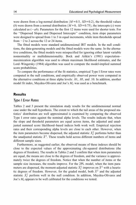
Type I Error Rates

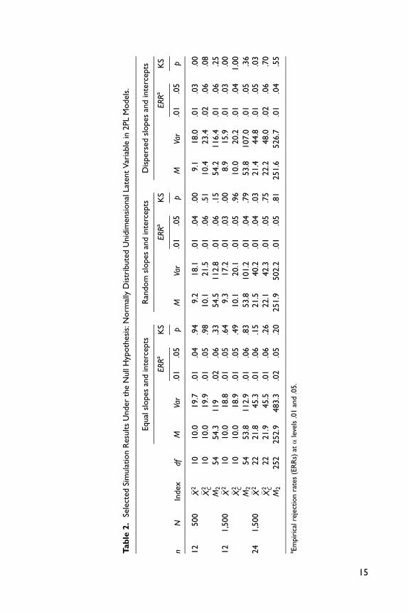
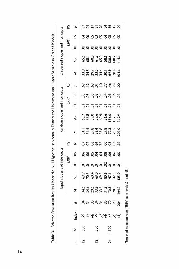
Tables 2 and 3 present the simulation study results for the unidimensional normal

case under the null hypothesis. The extent to which the tail areas of the proposed sta-

tistics’ distribution are well approximated is examined by comparing the observed

Type I error rates against the nominal alpha levels. The results indicate that, when

the slope and threshold parameters are equal across items, the adjusted and unad-

justed summed score likelihood–based indices both work well. Empirical rejection

rates and their corresponding alpha levels are close to each other. However, when

the item parameters become dispersed, the adjusted statistic �X 2C performs better than

the unadjusted statistic �X 2. These results hold across different numbers of items and

different sample sizes.

Furthermore, as suggested earlier, the observed means of these indexes should be

close to the expected values of the approximating chi-squared distributions (the

degrees of freedom). The results in Tables 2 and 3 confirm that when item parameters

are equal, the means are close to the degrees of freedom, and the variance is approxi-

mately twice the degrees of freedom. Notice that when the number of items or the

sample size increases, the results improve. For the 2PL model, when the item para-

meters are dispersed, the moment-adjusted statistic �X 2C improves on �X 2 with a heuris-

tic degrees of freedom. However, for the graded model, both �X 2 and the adjusted

statistic �X 2C perform well in the null condition. In addition, Maydeu-Olivares and

Joe’s M2 appears to be well calibrated for the conditions we tested.


Tab

le2.

Sele

cted

Sim

ula

tion

Res

ults

Under

the

Null

Hyp

oth

esis

:Norm

ally

Dis

trib

ute

dU

nid

imen

sional

Late

nt

Var

iable

in2PL

Model

s.

nN

Index

df

Equal

slopes

and

inte

rcep

tsR

andom

slopes

and

inte

rcep

tsD

isper

sed

slopes

and

inte

rcep

ts

MVa

r

ERR

aK

S

MVa

r

ERR

aK

S

MVa

r

ERR

aK

S

.01

.05

p.0

1.0

5p

.01

.05

p

12

500

� X2

10

10.0

19.7

.01

.04

.94

9.2

18.1

.01

.04

.00

9.1

18.0

.01

.03

.00

� X2 C

10

10.0

19.9

.01

.05

.98

10.1

21.5

.01

.06

.51

10.4

23.4

.02

.06

.08

M2

54

54.3

119

.02

.06

.33

54.5

112.8

.01

.06

.15

54.2

116.4

.01

.06

.25

12

1,5

00

� X2

10

10.0

18.8

.01

.05

.64

9.3

17.2

.01

.03

.00

8.9

15.9

.01

.03

.00

� X2 C

10

10.0

18.9

.01

.05

.49

10.1

20.1

.01

.05

.96

10.0

20.2

.01

.04

1.0

0M

254

53.8

112.

9.0

1.0

6.8

353.8

101.2

.01

.04

.79

53.8

107.0

.01

.05

.36

24

1,5

00

� X2

22

21.8

45.3

.01

.06

.15

21.5

40.2

.01

.04

.03

21.4

44.8

.01

.05

.03

� X2 C

22

21.9

45.5

.01

.06

.26

22.1

42.3

.01

.05

.75

22.2

48.0

.02

.06

.70

M2

252

252.9

483.

3.0

2.0

5.2

0251.

9502.2

.01

.05

.81

251.6

526.7

.01

.04

.55

a Em

pir

ical

reje

ctio

nra

tes

(ER

Rs)

ata

leve

ls.0

1an

d.0

5.

15

Tab

le3.

Sele

cted

Sim

ula

tion

Res

ults

Under

the

Null

Hyp

oth

esis

:Norm

ally

Dis

trib

ute

dU

nid

imen

sional

Late

nt

Var

iable

inG

raded

Model

s.

nN

Index

d

Equal

slopes

and

inte

rcep

tsR

andom

slopes

and

inte

rcep

tsD

isper

sed

slopes

and

inte

rcep

ts

MVa

r

ERR

aK

S

MVa

r

ERR

aK

S

MVa

r

ERR

aK

S

.01

.05

p.0

1.0

5p

.01

.05

p

12

500

� X2

34

34.5

69.9

.01

.06

.07

34.1

65.7

.01

.05

.67

33.8

65.6

.01

.04

.97

� X2 C

34

34.6

70.3

.01

.06

.02

34.4

66.8

.01

.05

.12

34.5

68.4

.01

.06

.04

M2

30

29.5

60.4

.01

.05

.06

29.8

59.0

.01

.05

.63

29.7

60.0

.01

.05

.17

12

1,5

00

� X2

34

33.8

69.0

.01

.04

.64

33.4

59.6

.01

.03

.01

33.5

61.8

.01

.03

.21

� X2 C

34

33.9

69.3

.01

.04

.75

33.8

60.9

.01

.04

.10

34.4

65.0

.01

.05

.26

M2

30

31.8

80.6

.02

.08

.00

29.8

56.6

.01

.04

.77

30.1

58.6

.01

.04

.24

24

1,5

00

� X2

70

70.9

147.

1.0

1.0

6.0

370.3

136.0

.01

.05

.46

69.9

138.6

.01

.05

.36

� X2 C

70

70.9

147.

3.0

1.0

6.0

370.5

137.1

.01

.06

.24

70.4

140.7

.01

.05

.15

M2

204

204.3

435.

9.0

1.0

6.5

8202.0

369.9

.01

.03

.00

204.6

414.6

.01

.05

.29

a Em

pir

ical

reje

ctio

nra

tes

(ER

Rs)

ata

leve

ls.0

1an

d.0

5.

16

Power

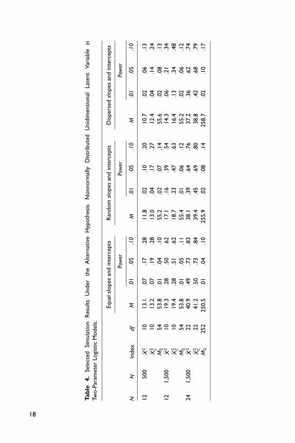
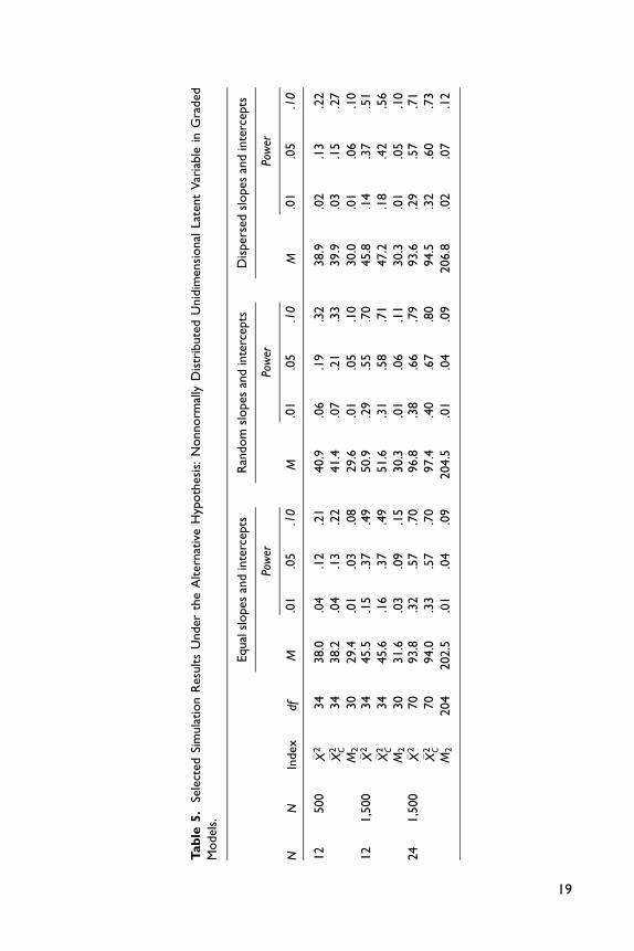
From Tables 4 and 5, it is clear that the summed score likelihood–based indices have

substantially higher power than M2 when the latent variable distribution is nonnor-

mal. The performance of the proposed statistics is heavily influenced by the number

of items and dispersion of item parameters. For both 2PL and graded models, the

power of the proposed indexes grow as the sample size and number of items increase.

This is to be expected as more data bring more information about the latent variable

distribution. When the item slope and threshold parameters are equal across items,

the unadjusted and adjusted statistics perform equally well. However, when the item

parameters are dispersed, the adjusted statistic �X 2C has higher power than the unad-

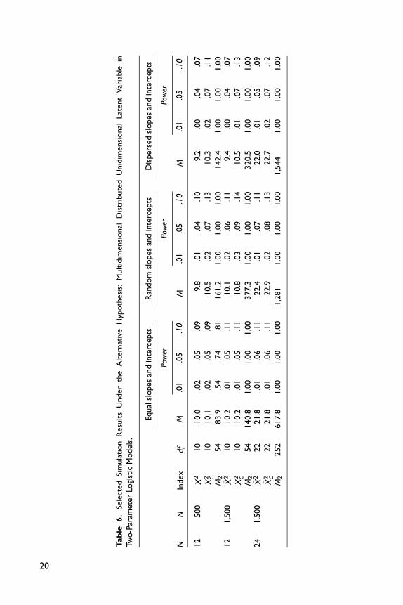
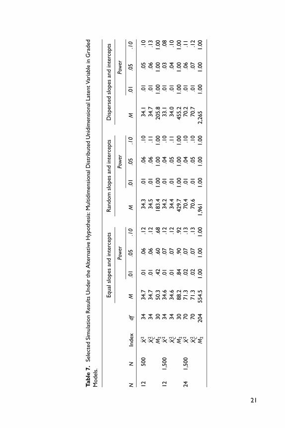
justed statistic �X 2. Finally, Tables 6 and 7 provide some evidence that the summed

score likelihood–based indices are not sensitive to model misspecification related to

multidimensionality, in contrast to M2. This is a desirable feature of the proposed

indices, which ought to be more targeted against specific forms of model misspecifi-

cation. M2 on the other hand, is a more general index for global model fit assessment.

An Application to Empirical Data

We illustrate the test statistics with empirical data. Twelve items related to positive

consequences of nicotine (Tucker et al., 2014), as part of a questionnaire dealing

with various attitudes, beliefs, and behaviors related to smoking (Shadel, Edelen, &

Tucker, 2011), were administered to a sample of 2,717 daily cigarette smokers. Each

item was rated on a 5-point ordinal scale. This study was part of the development of

the National Institute of Health’s Patient Reported Outcomes Measurement

Information System (PROMIS) and extensive item and dimensional analysis was

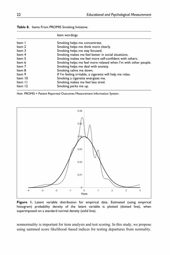
conducted prior to calibration of the items as unidimensional. The density plot

(Figure 1) of the latent variable distribution for this subscale shows its deviation from

a standard normal distribution that there are two maximum points in the middle

instead of a ‘‘bell curve’’ shape. Table 8 presents the contents of the 12 items from

the PROMIS smoking assessment.

Results show that when we use the normal unidimensional IRT model, �X 2 equals

to 208.5, and �X 2C equals to 179.3, indicating significant lack of latent variable normal-

ity (df = 46, p \ .0001). But when the empirical histogram latent density estimation

is used instead for item parameter estimation, �X 2 is equal to 51.2 and �X 2C is equal to

49.4 (df = 46, p . .1). In sum, we came to the conclusion that the latent variable dis-

tribution of this set of items was probably nonnormal and our proposed indices were

able to detect the violation of latent variable distribution assumption.

Discussion

Normality of latent variable distribution is a critical assumption in standard maximum

marginal likelihood estimation for IRT models. However, in real-world applications,

the distribution of latent variables can be nonnormal. The detection of latent variable

Li and Cai 17

Tab

le4.

Sele

cted

Sim

ula

tion

Res

ults

Under

the

Alter

nat

ive

Hyp

oth

esis

:N

onnorm

ally

Dis

trib

ute

dU

nid

imen

sional

Late

nt

Var

iable

inTw

o-P

aram

eter

Logi

stic

Model

s.

NN

Index

df

Equal

slopes

and

inte

rcep

tsR

andom

slopes

and

inte

rcep

tsD

isper

sed

slopes

and

inte

rcep

ts

M

Pow

er

M

Pow

er

M

Pow

er

.01

.05

.10

.01

.05

.10

.01

.05

.10

12

500

� X2

10

13.1

.07

.17

.28

11.8

.02

.10

.20

10.7

.02

.06

.13

� X2 C

10

13.2

.07

.19

.28

13.0

.04

.17

.27

12.4

.04

.14

.24

M2

54

53.8

.01

.04

.10

55.2

.02

.07

.14

55.6

.02

.08

.13

12

1,5

00

� X2

10

19.3

.28

.50

.62

17.1

.16

.39

.54

14.3

.06

.21

.34

� X2 C

10

19.4

.28

.51

.62

18.7

.23

.47

.63

16.4

.13

.34

.48

M2

54

53.8

.01

.05

.11

55.4

.01

.06

.12

55.2

.02

.06

.12

24

1,5

00

� X2

22

40.9

.49

.73

.83

38.1

.39

.64

.76

37.2

.36

.62

.74

� X2 C

22

41.2

.50

.73

.84

39.4

.45

.69

.80

38.8

.42

.68

.79

M2

252

250.5

.01

.04

.10

255.9

.02

.08

.14

258.7

.02

.10

.17

18

Tab

le5.

Sele

cted

Sim

ula

tion

Res

ults

Under

the

Alter

nat

ive

Hyp

oth

esis

:N

onnorm

ally

Dis

trib

ute

dU

nid

imen

sional

Late

nt

Var

iable

inG

raded

Model

s.

NN

Index

df

Equal

slopes

and

inte

rcep

tsR

andom

slopes

and

inte

rcep

tsD

isper

sed

slopes

and

inte

rcep

ts

M

Pow

er

M

Pow

er

M

Pow

er

.01

.05

.10

.01

.05

.10

.01

.05

.10

12

500

� X2

34

38.0

.04

.12

.21

40.9

.06

.19

.32

38.9

.02

.13

.22

� X2 C

34

38.2

.04

.13

.22

41.4

.07

.21

.33

39.9

.03

.15

.27

M2

30

29.4

.01

.03

.08

29.6

.01

.05

.10

30.0

.01

.06

.10

12

1,5

00

� X2

34

45.5

.15

.37

.49

50.9

.29

.55

.70

45.8

.14

.37

.51

� X2 C

34

45.6

.16

.37

.49

51.6

.31

.58

.71

47.2

.18

.42

.56

M2

30

31.6

.03

.09

.15

30.3

.01

.06

.11

30.3

.01

.05

.10

24

1,5

00

� X2

70

93.8

.32

.57

.70

96.8

.38

.66

.79

93.6

.29

.57

.71

� X2 C

70

94.0

.33

.57

.70

97.4

.40

.67

.80

94.5

.32

.60

.73

M2

204

202.5

.01

.04

.09

204.5

.01

.04

.09

206.8

.02

.07

.12

19

Tab

le6.

Sele

cted

Sim

ula

tion

Res

ults

Under

the

Alter

nat

ive

Hyp

oth

esis

:M

ultid

imen

sional

Dis

trib

ute

dU

nid

imen

sional

Late

nt

Var

iable

inTw

o-P

aram

eter

Logi

stic

Model

s.

NN

Index

df

Equal

slopes

and

inte

rcep

tsR

andom

slopes

and

inte

rcep

tsD

isper

sed

slopes

and

inte

rcep

ts

M

Pow

er

M

Pow

er

M

Pow

er

.01

.05

.10

.01

.05

.10

.01

.05

.10

12

500

� X2

10

10.0

.02

.05

.09

9.8

.01

.04

.10

9.2

.00

.04

.07

� X2 C

10

10.1

.02

.05

.09

10.5

.02

.07

.13

10.3

.02

.07

.11

M2

54

83.9

.54

.74

.81

161.2

1.0

01.0

01.0

0142.4

1.0

01.0

01.0

012

1,5

00

� X2

10

10.2

.01

.05

.11

10.1

.02

.06

.11

9.4

.00

.04

.07

� X2 C

10

10.2

.01

.05

.11

10.8

.03

.09

.14

10.5

.01

.07

.13

M2

54

140.8

1.0

01.0

01.0

0377.3

1.0

01.0

01.0

0320.5

1.0

01.0

01.0

024

1,5

00

� X2

22

21.8

.01

.06

.11

22.4

.01

.07

.11

22.0

.01

.05

.09

� X2 C

22

21.8

.01

.06

.11

22.9

.02

.08

.13

22.7

.02

.07

.12

M2

252

617.8

1.0

01.0

01.0

01,2

81

1.0

01.0

01.0

01,5

44

1.0

01.0

01.0

0

20

Tab

le7.

Sele

cted

Sim

ula

tion

Res

ults

Under

the

Alter

nat

ive

Hyp

oth

esis

:Multid

imen

sional

Dis

trib

ute

dU

nid

imen

sional

Late

nt

Var

iable

inG

raded

Model

s.

NN

Index

df

Equal

slopes

and

inte

rcep

tsR

andom

slopes

and

inte

rcep

tsD

isper

sed

slopes

and

inte

rcep

ts

M

Pow

er

M

Pow

er

M

Pow

er

.01

.05

.10

.01

.05

.10

.01

.05

.10

12

500

� X2

34

34.7

.01

.06

.12

34.3

.01

.06

.10

34.1

.01

.05

.10

� X2 C

34

34.7

.01

.06

.12

34.5

.01

.06

.11

34.7

.01

.06

.13

M2

30

50.3

.42

.60

.68

183.4

1.0

01.0

01.0

0205.8

1.0

01.0

01.0

012

1,5

00

� X2

34

34.6

.01

.07

.12

34.2

.01

.04

.10

33.1

.01

.03

.08

� X2 C

34

34.6

.01

.07

.12

34.4

.01

.05

.11

34.0

.01

.04

.10

M2

30

88.2

.84

.90

.92

429.7

1.0

01.0

01.0

0455.2

1.0

01.0

01.0

024

1,5

00

� X2

70

71.3

.02

.07

.13

70.4

.01

.04

.10

70.2

.01

.06

.11

� X2 C

70

71.3

.02

.07

.13

70.6

.01

.05

.10

70.7

.01

.07

.12

M2

204

554.5

1.0

01.0

01.0

01,9

61

1.0

01.0

01.0

02,2

65

1.0

01.0

01.0

0

21

nonnormality is important for item analysis and test scoring. In this study, we propose

using summed score likelihood–based indices for testing departures from normality.

Table 8. Items From PROMIS Smoking Initiative.

Item wordings

Item 1 Smoking helps me concentrate.Item 2 Smoking helps me think more clearly.Item 3 Smoking helps me stay focused.Item 4 Smoking makes me feel better in social situations.Item 5 Smoking makes me feel more self-confident with others.Item 6 Smoking helps me feel more relaxed when I’m with other people.Item 7 Smoking helps me deal with anxiety.Item 8 Smoking calms me down.Item 9 If I’m feeling irritable, a cigarette will help me relax.Item 10 Smoking a cigarette energizes me.Item 11 Smoking makes me feel less tired.Item 12 Smoking perks me up.

Note. PROMIS = Patient Reported Outcomes Measurement Information System.

Figure 1. Latent variable distribution for empirical data. Estimated (using empiricalhistogram) probability density of the latent variable is plotted (dotted line), whensuperimposed on a standard normal density (solid line).


We also develop a Satorra–Bentler type moment adjustment approach to approximate

the tail area probabilities of the indices.

In the simulation study, the performance of unadjusted and adjusted summed

score likelihood–based statistics was compared with that of M2. Results show that

the moment-adjusted index performs well for both dichotomous data and polytomous

data and maintains correct test size across number of items, sample size, and type of

IRT model considered. The unadjusted statistic does not work as well, especially

when item parameters are dispersed. Furthermore, the indices were particularly sen-

sitive to latent variable nonnormality, and not sensitive to other kinds of model misfit

such as multidimensionality.

An interesting finding is that the general goodness-of-fit statistic M2 (Maydeu-

Olivares & Joe, 2005) has almost no power against the nonnormal alternative, and

hence, cannot be recommended for testing latent variable distribution fit for IRT

models (see also Hansen, Cai, Monroe, & Li, 2016). This could be explained by the

observation that M2 is based only on first- and second-order margins of the underly-

ing contingency table, but to detect latent variable distributional misfit, information

from higher order margins may be necessary.

This study is not without its limitations. First, the distributions of the proposed

indices are not exactly chi-squared. In our study, their tail-area probabilities were

approximated to first order by a chi-squared variable with the availability of the item

parameter error covariance matrix and a Jacobian. We focus on the first-order correc-

tion due to its simplicity and the fact that we observed empirically that the results of

the second-order correction did not differ substantively from that of the first order. In

the future, higher order moments could be considered to improve the performance of

the adjusted statistics for situations that we have not examined. Second, only a lim-

ited number of null conditions and only two alternative population distributions were

tested in the simulations. More extensive simulations are needed to fully understand

the performance of the test statistics. Third, we only studied the properties of the sta-

tistics and the corrections under maximum likelihood estimation. In principle, one

could derive similar statistics under limited-information estimation (e.g., with

weighted least squares). Finally, this study only considered the conditions when item

response data are assumed to be unidimensional. Multidimensional IRT models

(MIRT, Reckase, 2009) should be considered in subsequent work. One particularly

popular model in educational and psychological research is the full-information item

bifactor model (Cai, Yang, & Hansen, 2011; Gibbons & Hedeker, 1992; Reise,

2012). In this model, all items load on a general dimension, and an item is permitted

to load on at most one specific dimension that influences nonoverlapping subsets of

items. This feature of bifactor models implies that there exists valuable relation

between an observed summed score and the distribution of the latent general dimen-

sion (Cai, 2015). This relation implies an opportunity to test the underlying assump-

tion about the distribution of general latent dimension with summed score

likelihood–based statistics.

Li and Cai 23

Appendix

A Modified Lord–Wingersky Algorithm for Jacobian Computations

Consider a test with n dichotomous items, calibrated by a two-parameter logistic item

response theory model. Recall that Ti 1juð Þ is item i’s traceline for Category 1

(Equation 1), with Ti 0juð Þ = 1 2 Ti 1juð Þ for Category 0. Theoretically, there should

be 2n response patterns. The response pattern is indicated by u = u1, . . . , unð Þ. Under

the assumption of items’ conditional independence, the likelihood for a response pat-

tern u can be expressed as L ujuð Þ =Qn

i = 1 Ti uijuð Þ. For n dichotomous items, the

summed score s ranges from 0 to n. S = n + 1 is the number of all possible summed

scores. Recall that u =Pn

i = 1 ui is a notational shorthand for the summed score associ-

ated with response u (see Equation 16). The likelihood for summed score s = 0, . . . , n

is defined as

L sjuð Þ=Xu = s

L ujuð Þ=Xs = u

Yn

i = 1

Ti uijuð Þ, ð27Þ

Clearly, the likelihood of a summed score s is the sum of all response pattern like-

lihoods for u = s. In Lord–Wingersky algorithm, the summed score likelihoods are

built up recursively, one at a time (Lord & Wingersky, 1984). Let Li sjuð Þ indicate

the likelihood for summed score s after item i has been added into the computation.

In the first step, two summed score likelihoods are computed based on the tracelines

of Item 1: L1 0juð Þ= T1 0juð Þ and L1 1juð Þ = T1 1juð Þ.In the second step, we have three summed score likelihoods based on the likeli-

hoods from Step 1 and tracelines of Item 2:

L2 0juð Þ= L1 0juð ÞT2 0juð Þ;

L2 1juð Þ= L1 1juð ÞT2 0juð Þ+ L1 0juð ÞT2 1juð Þ;

L2 2juð Þ= L1 1juð ÞT2 1juð Þ: ð28Þ

Suppose n items have been added. The likelihoods for summed scores 0, . . . , nð Þare

Ln 0juð Þ= Ln�1 0juð ÞTn 0juð Þ;

Ln sjuð Þ= Ln�1 sjuð ÞTn 0juð Þ+ Ln�1 s� 1juð ÞTn 1juð Þ;

Ln njuð Þ= Ln�1 n� 1juð ÞTn 1juð Þ: ð29Þ

To obtain the Jacobian matrix of summed score likelihoods with respective to item

parameters, the Lord–Wingersky algorithm is adapted slightly. As previously men-

tioned, in the first step, there are only two summed score likelihoods based on Item

1: L1 0juð Þ and L1 1juð Þ. The first-order derivatives of summed score likelihoods with

respect to a generic item parameter g1 for Item 1 are


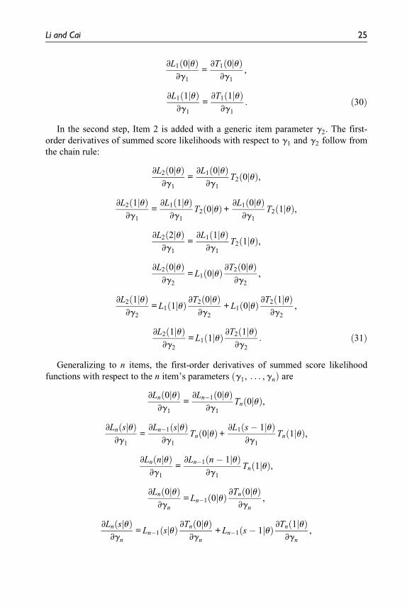
∂L1 0juð Þ∂g1

=∂T1 0juð Þ

∂g1

,

∂L1 1juð Þ∂g1

=∂T1 1juð Þ

∂g1

: ð30Þ

In the second step, Item 2 is added with a generic item parameter g2. The first-

order derivatives of summed score likelihoods with respect to g1 and g2 follow from

the chain rule:

∂L2 0juð Þ∂g1

=∂L1 0juð Þ

∂g1

T2 0juð Þ,

∂L2 1juð Þ∂g1

=∂L1 1juð Þ

∂g1

T2 0juð Þ+ ∂L1 0juð Þ∂g1

T2 1juð Þ,

∂L2 2juð Þ∂g1

=∂L1 1juð Þ

∂g1

T2 1juð Þ,

∂L2 0juð Þ∂g2

= L1 0juð Þ ∂T2 0juð Þ∂g2

,

∂L2 1juð Þ∂g2


+ L1 0juð Þ ∂T2 1juð Þ∂g2

,

∂L2 1juð Þ∂g2


: ð31Þ

Generalizing to n items, the first-order derivatives of summed score likelihood

functions with respect to the n item’s parameters g1, . . . , gnð Þ are

∂Ln 0juð Þ∂g1

=∂Ln�1 0juð Þ

∂g1

Tn 0juð Þ,

∂Ln sjuð Þ∂g1

=∂Ln�1 sjuð Þ

∂g1

Tn 0juð Þ+ ∂L1 s� 1juð Þ∂g1

Tn 1juð Þ,

∂Ln njuð Þ∂g1

=∂Ln�1 n� 1juð Þ

∂g1

Tn 1juð Þ,

∂Ln 0juð Þ∂gn

= Ln�1 0juð Þ ∂Tn 0juð Þ∂gn

,

∂Ln sjuð Þ∂gn

= Ln�1 sjuð Þ ∂Tn 0juð Þ∂gn

+ Ln�1 s� 1juð Þ ∂Tn 1juð Þ∂gn

,

Li and Cai 25

∂Ln njuð Þ∂gn

= Ln�1 n� 1juð Þ ∂Tn 1juð Þ∂gn

: ð32Þ

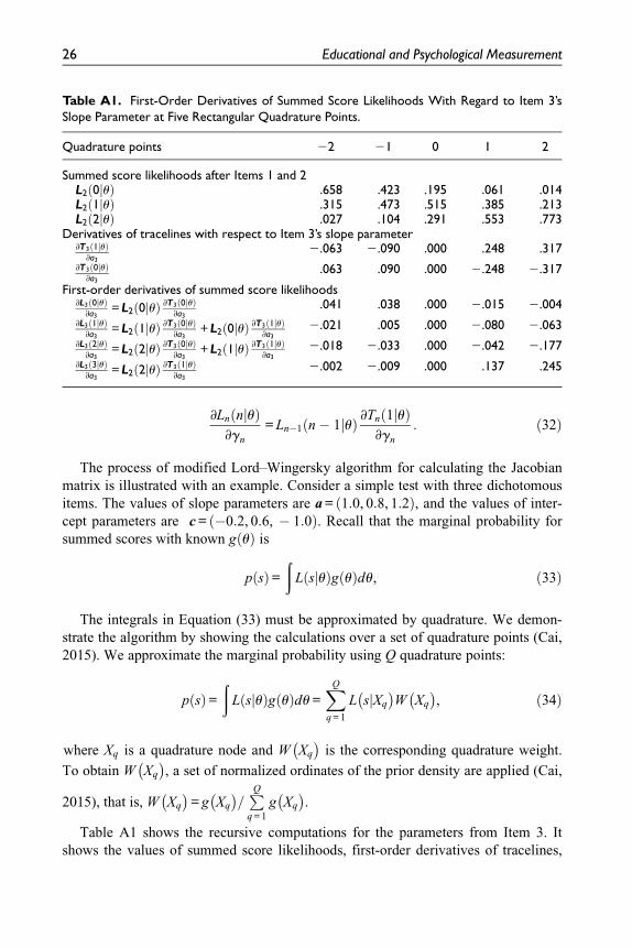
The process of modified Lord–Wingersky algorithm for calculating the Jacobian

matrix is illustrated with an example. Consider a simple test with three dichotomous

items. The values of slope parameters are a = 1:0, 0:8, 1:2ð Þ, and the values of inter-

cept parameters are c = �0:2, 0:6, � 1:0ð Þ. Recall that the marginal probability for

summed scores with known g uð Þ is

p sð Þ=ð

L sjuð Þg uð Þdu, ð33Þ

The integrals in Equation (33) must be approximated by quadrature. We demon-

strate the algorithm by showing the calculations over a set of quadrature points (Cai,

2015). We approximate the marginal probability using Q quadrature points:

p sð Þ=ð

L sjuð Þg uð Þdu =XQ

q = 1

L sjXq

� �W Xq

� �, ð34Þ

where Xq is a quadrature node and W Xq

� �is the corresponding quadrature weight.

To obtain W Xq

� �, a set of normalized ordinates of the prior density are applied (Cai,

2015), that is, W Xq

� �= g Xq

� �=PQq = 1

g Xq

� �.

Table A1 shows the recursive computations for the parameters from Item 3. It

shows the values of summed score likelihoods, first-order derivatives of tracelines,

Table A1. First-Order Derivatives of Summed Score Likelihoods With Regard to Item 3’sSlope Parameter at Five Rectangular Quadrature Points.

Quadrature points 22 21 0 1 2

Summed score likelihoods after Items 1 and 2L2 0juð Þ .658 .423 .195 .061 .014L2 1juð Þ .315 .473 .515 .385 .213L2 2juð Þ .027 .104 .291 .553 .773

Derivatives of tracelines with respect to Item 3’s slope parameter∂T3 1juð Þ

∂a3

2.063 2.090 .000 .248 .317

∂T3 0juð Þ∂a3

.063 .090 .000 2.248 2.317

First-order derivatives of summed score likelihoods∂L3 0juð Þ

∂a3= L2 0juð Þ ∂T3 0juð Þ

∂a3

.041 .038 .000 2.015 2.004

∂L3 1juð Þ∂a3

= L2 1juð Þ ∂T3 0juð Þ∂a3

+ L2 0juð Þ ∂T3 1juð Þ∂a3

2.021 .005 .000 2.080 2.063

∂L3 2juð Þ∂a3


+ L2 1juð Þ ∂T3 1juð Þ∂a3

2.018 2.033 .000 2.042 2.177

∂L3 3juð Þ∂a3


2.002 2.009 .000 .137 .245


and the first-order derivatives of summed score likelihoods at five equally spaced

quadrature points ( Q = 5): 22, 21, 0, 1, and 2. More quadrature points should be

used for better precision (Cai, 2015). The first block presents the summed score like-

lihoods after the first and second items are added in. The second block presents the

first-order derivatives of Item 3’s tracelines with respect to its slope parameter. The

third block presents the first-order derivatives of summed score likelihoods with

respect to Item 3’s slope parameter.

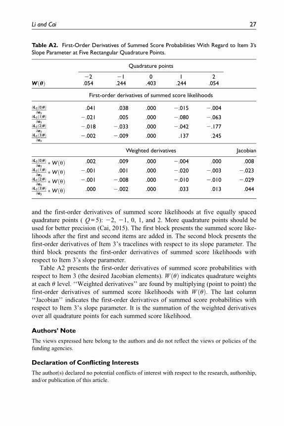
Table A2 presents the first-order derivatives of summed score probabilities with

respect to Item 3 (the desired Jacobian elements). W uð Þ indicates quadrature weights

at each u level. ‘‘Weighted derivatives’’ are found by multiplying (point to point) the

first-order derivatives of summed score likelihoods with W uð Þ. The last column

‘‘Jacobian’’ indicates the first-order derivatives of summed score probabilities with

respect to Item 3’s slope parameter. It is the summation of the weighted derivatives

over all quadrature points for each summed score likelihood.

Authors’ Note

The views expressed here belong to the authors and do not reflect the views or policies of the

funding agencies.

Declaration of Conflicting Interests

The author(s) declared no potential conflicts of interest with respect to the research, authorship,

and/or publication of this article.

Table A2. First-Order Derivatives of Summed Score Probabilities With Regard to Item 3’sSlope Parameter at Five Rectangular Quadrature Points.

Quadrature points

22 21 0 1 2W uð Þ .054 .244 .403 .244 .054

First-order derivatives of summed score likelihoods

∂L3 0juð Þ∂a3

.041 .038 .000 2.015 2.004

∂L3 1juð Þ∂a3

2.021 .005 .000 2.080 2.063

∂L3 2juð Þ∂a3

2.018 2.033 .000 2.042 2.177

∂L3 3juð Þ∂a3

2.002 2.009 .000 .137 .245

Weighted derivatives Jacobian

∂L3 0juð Þ∂a3�W uð Þ .002 .009 .000 2.004 .000 .008

∂L3 1juð Þ∂a3�W uð Þ 2.001 .001 .000 2.020 2.003 2.023

∂L3 2juð Þ∂a3�W uð Þ 2.001 2.008 .000 2.010 2.010 2.029

∂L3 3juð Þ∂a3�W uð Þ .000 2.002 .000 .033 .013 .044

Li and Cai 27

Funding

The author(s) disclosed receipt of the following financial support for the research, authorship,

and/or publication of this article: Part of this research was supported by the Institute of

Education Sciences (R305D140046).

References

Bartholomew, D. J., & Tzamourani, P. (1999). The goodness-of-fit of latent trait models in

attitude measurement. Sociological Methods and Research, 27, 525-546.

Bishop, Y. M. M., Fienberg, S. E., & Holland, P. W. (1975). Discrete multivariate analysis:

Theory and practice. Cambridge, MA: MIT Press.

Bock, R. D., & Aitkin, M. (1981). Marginal maximum likelihood estimation of item

parameters: Application of an EM algorithm. Psychometrika, 46, 443-459.

Bock, R. D., & Lieberman, M. (1970). Fitting a response model for n dichotomously scored

items. Psychometrika, 35, 179-197.

Cai, L. (2013). flexMIRT� version 2: Flexible multilevel item factor analysis and test scoring

[Computer software]. Chapel Hill, NC: Vector Psychometric Group.

Cai, L. (2015). Lord-Wingersky algorithm version 2.0 for hierarchical item factor models with

applications in test scoring, scale alignment, and model fit testing. Psychometrika, 80,

535-559.

Cai, L., & Hansen, M. (2013). Limited-information goodness-of-fit testing of hierarchical item

factor models. British Journal of Mathematical and Statistical Psychology, 66, 245-276.

Cai, L., Maydeu-Olivares, A., Coffman, D. L., & Thissen, D. (2006). Limited-information

goodness-of-fit testing of item response theory models for sparse 2P tables. British Journal

of Mathematical and Statistical Psychology, 59, 173-194.

Cai, L., Yang, J., & Hansen, M. (2011). Generalized full-information item bifactor analysis.

Psychological Methods, 16, 221-248.

Chen, W. H., & Thissen, D. (1997). Local dependence indices for item pairs using item

response theory. Journal of Educational and Behavioral Statistics, 22, 265-289.

Chen, W. H., & Thissen, D. (1999). Estimation of item parameters for the three-parameter

logistic model using the marginal likelihood of summed scores. British Journal of

Mathematical and Statistical Psychology, 52, 19-37.

Ferrando, P. J., & Lorenzo-seva, U. (2001). Checking the appropriateness of item response

theory models by predicting the distribution of observed scores: The program EO-fit.

Educational and Psychological Measurement, 61, 895-902.

Gibbons, R., & Hedeker, D. (1992). Full-information item bifactor analysis. Psychometrika,

57, 423-436.

Hambleton, R. K., & Traub, R. E. (1973). Analysis of empirical data using two logistic latent

trait models. British Journal of Mathematical and Statistical Psychology, 26, 195-211.

Hansen, M., Cai, L., Monroe, S., & Li, Z. (2016). Limited-information goodness-of-fit testing

of diagnostic classification item response models. British Journal of Mathematical and

Statistical Psychology, 69, 225-252.

Joe, H., & Maydeu-Olivares, A. (2010). A general family of limited information goodness-of-

fit statistics for multinomial data. Psychometrika, 75, 393-419.

Li, Z., & Cai, L. (2012, July). Summed score based fit indices for testing latent variable

distribution assumption in IRT. Paper presented at the 2012 International Meeting of the

Psychometric Society, Lincoln, NE.


Lord, F. M. (1953). The relation of test score to the latent trait underlying the test. Educational

and Psychological Measurement, 13, 517-548.

Lord, F. M., & Wingersky, M. S. (1984). Comparison of IRT true-score and equipercentile

observed-score ‘‘equatings.’’ Applied Psychological Measurement, 8, 453-461.

Mathai, A. M., & Provost, S. B. (1992). Quadratic forms in random variables: Theory and

applications. New York, NY: Marcel Dekker.

Maydeu-Olivares, A., & Cai, L. (2006). A cautionary note on using G2(dif) to assess relative

model fit in categorical data analysis. Multivariate Behavioral Research, 41, 55-64.

Maydeu-Olivares, A., & Joe, H. (2005). Limited and full information estimation and testing in

2n contingency tables: A unified framework. Journal of the American Statistical

Association, 100, 1009-1020.

Maydeu-Olivares, A., & Joe, H. (2006). Limited information goodness-of-fit testing in

multidimensional contingency tables. Psychometrika, 71, 713-732.

Mislevy, R. (1984). Estimating latent distributions. Psychometrika, 49, 359-381.

Monroe, S. (2014). Multidimensional item factor analysis with semi-nonparametric latent

densities (Unpublished doctoral dissertation). University of California, Los Angeles.

Monroe, S., & Cai, L. (2014). Estimation of a Ramsay-curve item response theory model by

the Metropolis-Hastings Robbins-Monro Algorithm. Educational and Psychological

Measurement, 42, 343-369.

Orlando, M., & Thissen, D. (2000). Likelihood-based item-fit indices for dichotomous item

response theory models. Applied Psychological Measurement, 24, 50-64.

Reckase, M. (2009). Multidimensional item response theory (statistics for social and

behavioral sciences). New York, NY: Springer.

Reise, S. (2012). The rediscovery of bifactor measurement models. Multivariate Behavioral

Research, 47, 667-696.

Ross, J. (1966). An empirical study of a logistic mental test model. Psychometrika, 31,

325-340.

Satorra, A., & Bentler, P. M. (1994). Corrections to test statistics and standard errors in

covariance structure analysis. In A. von Eye & C. C. Clogg (Eds.), Latent variables

analysis: Applications for developmental research (pp. 399-419). Thousand Oaks, CA:

Sage.

Shadel, W. G., Edelen, M., & Tucker, J. S. (2011). A unified framework for smoking

assessment: The PROMIS Smoking Initiative. Nicotine & Tobacco Research, 13, 399-400.

Sinharay, S., Johnson, M. S., & Stern, H. S. (2006). Posterior predictive assessment of item

response theory models. Applied Psychological Measurement, 30, 298-321.

Thissen, D., & Steinberg, L. (2009). Item response theory. In R. Millsap & A. Maydeu-

Olivares (Eds.), The Sage handbook of quantitative methods in psychology (pp. 148-177).

London, England: Sage.

Thissen, D., & Wainer, H. (2001). Test scoring. Hillsdale, NJ: Lawrence Erlbaum.

Tucker, J., Shadel, W. G., Stucky, B., Cerully, J., Li, Z., Hansen, M., & Cai, L. (2014).

Development of the PROMIS positive emotional and sensory expectancies of smoking

item banks. Nicotine and Tobacco Research, 16(Suppl. 3), S212-S222.

van der Ark, L. A. (2005). Stochastic ordering of the latent trait by the sum score under various

polytomous IRT models. Psychometrika, 70, 283-304.

Woods, C. M. (2006). Ramsay-curve item response theory to detect and correct for non-normal

latent variables. Psychological Methods, 11, 253-270.

Li and Cai 29

Woods, C. M., & Lin, N. (2009). Item response theory with estimation of the latent density

using Davidian curves. Applied Psychological Measurement, 33, 102-117.

Woods, C. M., & Thissen, D. (2006). Item response theory with estimation of the latent

population distribution using spline-based densities. Psychometrika, 71, 281-301.

Zimowski, M. F., Muraki, E., Mislevy, R. J., & Bock, R. D. (1996). BILOG-MG: Multiple-

group IRT analysis and test maintenance for binary items [Computer software].

Lincolnwood, IL: Scientific Software International.


Documents

Summed Score Likelihood–