Embed Size (px)
Citation preview
mathematics of computationvolume 64, number 212october 1995, pages 1473-1493
SUMMATION BY PARTS, PROJECTIONS, AND STABILITY. II
PELLE OLSSON
Abstract. In this paper we prove strict stability of high-order finite difference
approximations of parabolic and symmetric hyperbolic systems of partial dif-
ferential equations on bounded, curvilinear domains in two space dimensions.
The boundary need not be smooth. We also show how to derive strict stability
estimates for inhomogeneous boundary conditions.
1. Strict stability in several space dimensions
In [2] we proved stability for high-order finite difference approximations of
hyperbolic and parabolic systems using certain projections and difference oper-ators satisfying a summation-by-parts rule. In one space dimension we showed
how to obtain strict stability. The aim of this paper is to prove strict stability
in several space dimensions. Furthermore, it will also be demonstrated how to
handle inhomogeneous boundary conditions. We limit ourselves to two space
dimensions for convenience.
The purpose of strict stability is to ensure the same growth rate of the dis-crete and analytic solutions. If the analytic problem is defined on a curvilinear
domain Q with boundary Y (cf. Fig. 1 on next page), then there must exist a
diffeomorphism Ç = Ç(x) of Q, onto the unit square (0, 1) x (0, 1) in order
for the finite difference method to be well defined. Consequently, a constant-
coefficient problem in the original domain may be transformed to a variable-
coefficient problem on the unit square, which may account for a nonphysical
growth in the discrete estimate.
Let £ = Ç(x) be a diffeomorphism of Í2 onto / = (0, 1) x (0, 1). Thefollowing identities are readily established:
aix dx2 ' dtx(l.i)
Ö£l _r-xHl_ 3*2
d& dx2 ' ö{2
which in turn implies
(1-2) £ (/;=1
Received by the editor January 19, 1994 and, in revised form, August 5, 1994.
1991 Mathematics Subject Classification. Primary 65M06, 65M12.This work has been sponsored by NASA under contract No. NAS 2-13721.
©1995 American Mathematical Society
1473
= -Jdx, '
/dx, '
,-wg
ldii) =o,
License or copyright restrictions may apply to redistribution; see http://www.ams.org/journal-terms-of-use
1474 PELLE OLSSON
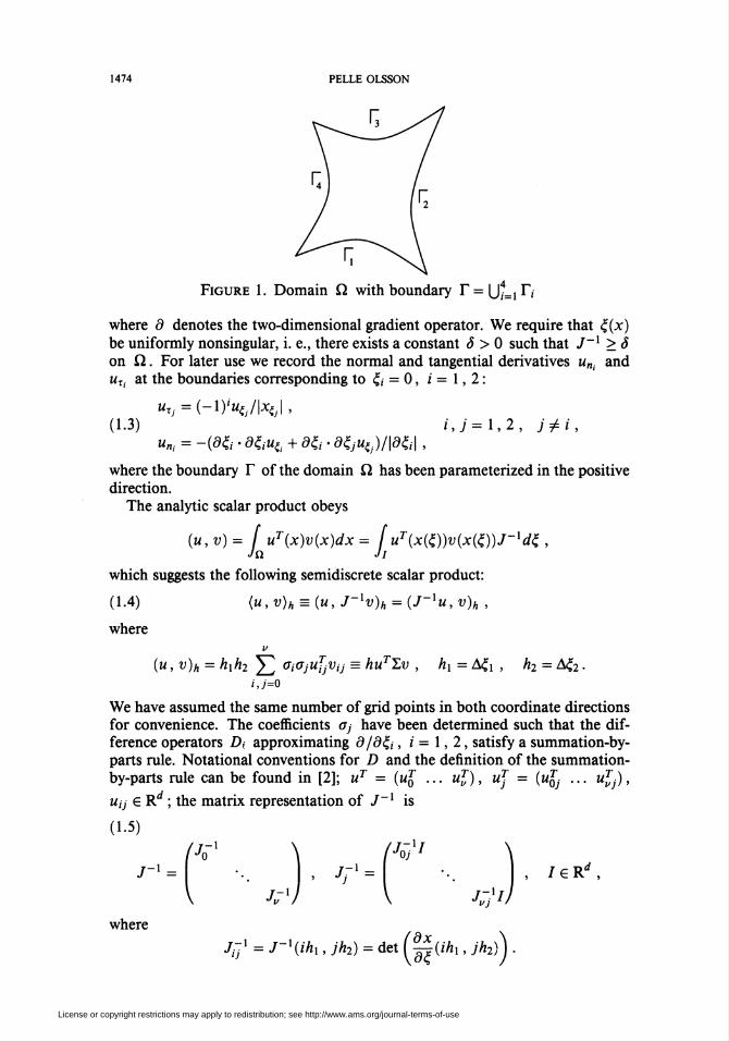
Figure 1. Domain Q with boundary r=U*=ir,-
where d denotes the two-dimensional gradient operator. We require that Ç(x)
be uniformly nonsingular, i. e., there exists a constant ô > 0 such that J~x > S
on Q. For later use we record the normal and tangential derivatives un¡ anduT. at the boundaries corresponding to & = 0, i = 1, 2 :
UT. =(-l)'Mí./|xí.| ,
(1.3) i,j=l,2, j¿i,
un¡ = -(oí,- • díiu(l + deli ■ dZjU^/idtii,
where the boundary Y of the domain Q has been parameterized in the positive
direction.
The analytic scalar product obeys
(u,v)= I uT(x)v(x)dx= luT(x(cl))v(x(cl))J-xdc:,Ja Ji
which suggests the following semidiscrete scalar product:
(1.4) (u, v)h = (u, J~lv)h = (J~xu, v)h ,
where
(u, v)h = hxh2 J2 OiOjuJjVij s huTY7u , hx = AÇX , h2 = A£2.¿,7=0
We have assumed the same number of grid points in both coordinate directionsfor convenience. The coefficients 07 have been determined such that the dif-
ference operators D¡ approximating d/dÇj, ¿=1,2, satisfy a summation-by-parts rule. Notational conventions for D and the definition of the summation-
by-parts rule can be found in [2]; uT = (uT ... uT), uj = (ufij ... uT^,
Uij £ Rd ; the matrix representation of J~x is
(1.5)
Mr1 \ /V/-'= -,
V jv-1J
where
•uj I
v= 7eRd,
V K}i>
J-jX = J~x(ihx, jh2) = det (jf(ihi, jh2)}
License or copyright restrictions may apply to redistribution; see http://www.ams.org/journal-terms-of-use
SUMMATION BY PARTS, PROJECTIONS, AND STABILITY. II 1475
Similarly,
(1.6)<o0I.o \ /o0I \
X= •.. , lj = •.. , ; = 0, ... , u.
\ <7„I„/ \ ovl)
Thus, each grid point in ( 1.4) is scaled with the cell volume.
The analytic boundary integrals can be parameterized as
/ uT(x)v(x)ds = / uT(x(c:x, 0))V(X((1 , 0))|jfc(& , 0)1^! .Jr¡ Jo
Hence, it is natural to define the boundary scalar product as
(1.7)V V
(u ,v)r = J2 Oj (sojuljVoj + svjuTjVuj) + ^ ct, {s¡ou[0vi0 + sivujvviv) ,
7=0 1=0
where the arc lengths are defined as
soj = \xi2(0, jh2)\h2 , 5,0 = \xix(ihx, Q)\hx ,
with similar definitions for sVj and s¡„ .
It was shown in [2, §2. 2] that the projection P representing the analytic
boundary conditions can be written as
(1.8) P = I-IrxL(LT"L-xL)-xLT ,
where L is the discretization of the analytic boundary operator. It follows that
(u, Pv)n = (Pu, v)n. It suffices to consider solutions that are supported only
in a neighborhood of (xx (0, 0), x2(0, 0)) ; P is assumed to be independent oft. In two space dimensions the general form of L is
(1.9) L=(LX0 ... LXr L20 ... L2r)£R^ldx2^d,
where L17 and L2i denote the boundary operators at x(0, jh2) and x(ihx, 0) ;
r is a constant depending on the approximation order of the boundary condi-
tions (typically the number of grid points along a coordinate line involved in
the approximation of the normal derivative). However, r does not depend onthe mesh sizes hx , h2. Furthermore,
L{j=(o ... 0 Y^MjkeTk 0 ... o|eR^+')\
Ll=(Ni0e[ ... NireJ 0 ... 0) £Rdx{u+l)2d.
Here, ef = (0 ... 0 / 0 ... 0) £ Rdx^+X)d , Mjk, Nik £ Rdxd .
In order to prove stability, we must have Pv = v. Since v will be the
solution of equations like (1.13), it follows that PJ~xv = J~xv . Therefore, itis natural to require
(1.10) pj-x = j~xp.
License or copyright restrictions may apply to redistribution; see http://www.ams.org/journal-terms-of-use
1476 PELLE OLSSON
For a general P this identity expresses a compatibility condition between the
analytic boundary conditions and the mapping £(x). Let P be given by (1.8)
and (1.9). Then (1.10) certainly holds if
(111) JU = J(x(ini'Jh2)) = Jio, i = 0,...,v, j = 0,...,r,Ju = J(x(ihx, jh2)) = J0j, i = 0,... , r , j = 0,... , v ,
which states that the mapping Ç(x) is locally isochoric, i. e., volume preserving,
in the x^-direction at the boundary, where d/dC¡ is the nontangential deriva-
tive. In case of characteristic boundary conditions and Dirichlet conditions we
have r = 0, and (1.11) is trivially satisfied. For general boundary conditions,
however, (1.11) couples the boundary operator to the grid transformation.
1.1. Symmetric hyperbolic systems. Using (1.2), we recast
2
ut = Y^ AiUx, + F , xg£î, Aj = Ai ,i=i
into a form that eliminates the need for the commutator in the semidiscrete
case
(1.12)
(j~lu)t = i¿ (([j-lBiUJ + J-lBiUt) - ^J~xdiv(A)u + J~XF ,
where
Bi-K-A-gLAr + gLAt, div(A) = d -A = ^ + ^ .dxx dx2 dX[ dx2
Define the characteristic variables as <p(x, t) = QT(x)u(x, t) , x £ Y, where
Q are the orthogonal eigenvectors (assumed to be time-independent) of B =
nxAx + n2A2 ; n is the outward unit normal at Y. At each boundary point Xy it
is assumed that the eigenvalues of B(x¡j) satisfy |¿(-X/_/)| > y¡j ', the significance
of this assumption is explained in [2, §§3. 1, 4. 1]. The characteristic boundary
conditions can then be expressed as
fi(x, t) = S(x)(pu(x, t) ,
where S(x) is assumed to be "small"; <pi(x, t), <p¡¡(x, t) denote the in- and
outgoing characteristic variables. In the original variables we thus have
L(x)u(x, t) = (Of (x) - S(x)Qj,(x))u(x, 0 = 0, x £ Y.
The smallness assumption on S(x) implies that L(x) has full rank. At the
corner xoo = *(0, 0) we require that the characteristic boundary conditions
be satisfied for <p(x0o, t) = Qf (*oo)u(xoo, t), i = 1,2, where Q¡ are the
eigenvectors of B(x0o), n = n(l) = -9^,/|ö^| being the two normals at the
License or copyright restrictions may apply to redistribution; see http://www.ams.org/journal-terms-of-use
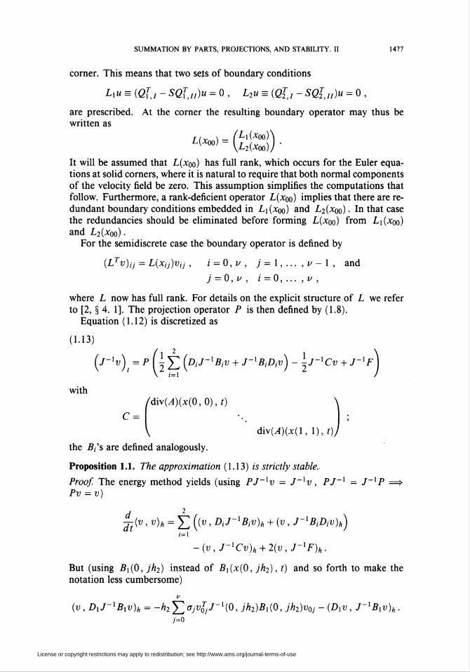
SUMMATION BY PARTS, PROJECTIONS, AND STABILITY. II 1477
corner. This means that two sets of boundary conditions
Lxu = (Qfj - SQTXJI)u = 0 , L2u = (Qlj - SQlM)u = 0 ,
are prescribed. At the corner the resulting boundary operator may thus be
written as
L(xoo) = ( L■£*iCxoo)\
2(*00)7
It will be assumed that L(xqo) has full rank, which occurs for the Euler equa-
tions at solid corners, where it is natural to require that both normal components
of the velocity field be zero. This assumption simplifies the computations that
follow. Furthermore, a rank-deficient operator L(xoo) implies that there are re-
dundant boundary conditions embedded in Lx(xqo) and L2(x0o) ■ In that case
the redundancies should be eliminated before forming L(xoo) from Lx(x0o)
and L2(xoo)-For the semidiscrete case the boundary operator is defined by
(LTv)ij = L(Xij)Vij , i = 0, v , j = 1,... , v - 1 , and
; = 0, v , i = 0,... ,v ,
where L now has full rank. For details on the explicit structure of L we refer
to [2, § 4. 1]. The projection operator P is then defined by (1.8).
Equation (1.12) is discretized as
(1.13)
(y-'w) = P {^^(DiJ-1 Bv + J~x BiDiv) -X-J~xCv + J-xf\
with
/div(^)(x(0,0),í) \
c= ■■. ;V div(A)(x(l,l),t)J
the B7s are defined analogously.
Proposition 1.1. The approximation (1.13) is strictly stable.
Proof. The energy method yields (using PJ~xv = J~xv, PJ~X = J~XP =4>Pv = v)
, 2
Tt(v ,v)k = Y, ((v , DiJ-xBiV)h + (v , J-xBiDiV)h)df i=\
-(v,J-iCv)h + 2(v,J-iF)h.
But (using ¿?i(0, jh2) instead of Bx(x(0, jh2), t) and so forth to make the
notation less cumbersome)
V
(v,DxJ~xBxv)h = -h2Y,<*jVojJ~l(0> Jh2)Bx(0, jh2)v0j - (Dxv , J~lBxv)h.
7=0
License or copyright restrictions may apply to redistribution; see http://www.ams.org/journal-terms-of-use
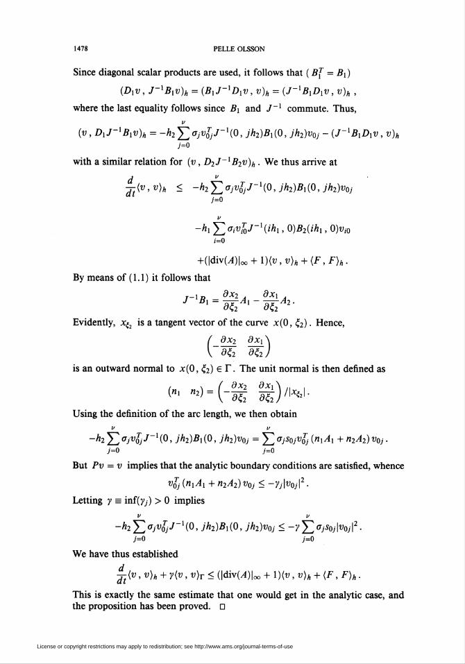
1478 PELLE OLSSON
Since diagonal scalar products are used, it follows that ( Bf = Bx )
(Dxv, J~xBxv)h = (BxJ-lDxv, v)h = (J-xBxDxv , v)h ,
where the last equality follows since Bx and J~x commute. Thus,
(v,DxJ-xBxv)n = -h2J2<TjvlJ-x(0, jh2)Bx(0, jh2)vQj - (J~xBxDxv , v)h7=0
with a similar relation for (v, D2J~xB2v)h . We thus arrive at
¿¡(v>v)h < -h2J2aJvojJ~l(°>Jh2)Bx(0,jh2)voj7=0
-hx ^2 aivïoJ \ih\ » Q)B2(ihx, 0)vi0i=0
+(\div(A)\oc + l)(v,v)h + (F,F)h.
By means of ( 1.1 ) it follows that
J~ Bx = -rj-^i - ~^rA2 ■dç2 dç2
Evidently, x¡2 is a tangent vector of the curve x(0,C2). Hence,
(_dx2 dxx\
\ dÇ2 dÇ2/
is an outward normal to x(0, Ç2) e Y. The unit normal is then defined as
, , / dx2 dxx\
Using the definition of the arc length, we then obtain
V V
-h2 J2 o~jVojJ~x(0, jh2)Bx(0, jh2)voj = J2 aJsoj^oj (*\¿\ + «2^2) v0J.7=0 7=0
But Pv = v implies that the analytic boundary conditions are satisfied, whence
vfj (nxAx + n2A2) v0j < -7j\v0j\2 ■
Letting y = inf(jj) > 0 implies
V V
-Ä2 5^ff/«oDv-1(0, jh2)Bx(0, jh2)v0j < -yY^ojSoj\voj\2 ■7=0 7=0
We have thus established
j-t(v, v)h + y(v , v)T < (Idiv^U + l)(v , v)h + (F, F)h .
This is exactly the same estimate that one would get in the analytic case, andthe proposition has been proved. 0
License or copyright restrictions may apply to redistribution; see http://www.ams.org/journal-terms-of-use
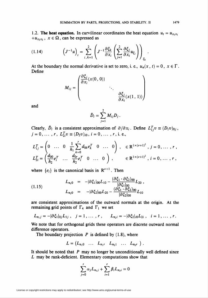
SUMMATION BY PARTS, PROJECTIONS, AND STABILITY. II 1479
1.2. The heat equation. In curvilinear coordinates the heat equation ut = ux¡x¡
+uX2x2, x £Q, can be expressed as
(1.14) H,-.çMiteîhAt the boundary the normal derivative is set to zero, i. e., u„(x, t) = 0, x £Y.
Define
(d_kdXi
Mij =
(x(0, 0))
gwi.oyand
bi = YéMijDj.7=1
Clearly, D¡ is a consistent approximation of d/dxj. Define LjjV = (Dxv)oj
7 = 0, ... , r, LT(v = (D2v)io, J = 0, ... , r,i. e.,
Ll = ° • 0 ^-¿^e,r 0 ... o) , £RXx^\j = 0,
1 k=0 /
LT2i={^eJ ... ^ej 0 ... o), e Rlx("+1)2 , i = 0,.
where {e¡} is the canonical basis in R1^1 . Then
r ,
(1.15)Ln,o — -|cçi loo-^io-râË~i-^20,
|Cçi|oo
-|CÇ2|00-t-20-rôë~l--M0J«20
|oí:2100
are consistent approximations of the outward normals at the origin. At theremaining grid points of T4 and Yx we set
Ln,j = -|0£i \ojLXj , j = 1, ... , r , L„2i = -\dC2\ioL2i , i-1, ... ,r.
We note that for orthogonal grids these operators are discrete outward normal
difference operators.
The boundary projection P is defined by (1.8), where
L = (L„lC l^n^r *-•n2\ En2r ) ■
It should be noted that P may no longer be unconditionally well defined since
L may be rank-deficient. Elementary computations show that
r r
^2 aJLnd + Y^ &L"2' = °7=0 i=l
License or copyright restrictions may apply to redistribution; see http://www.ams.org/journal-terms-of-use

1480 PELLE OLSSON
implies
(|Ô{i|§oA2 + (ôi1-ai2)ooAi)ao = 0.
If (dt;x • d¡í2)oo < 0, i. e., at acute corners, there is a possibility of a nonzero
o-o if
(1.16) h2~ 'ldW~hl ■
Hence, at acute corners we assume hx and h2 to be such that (1.16) does nothold. Furthermore,
L — (L/1,0 L„lX ••■ L„¡r L„2o L„2i ... L„27)
is rank-deficient. This is obvious if d£,x • dÇ2 - ±\dÇx\\dÇ2\, because thenL„,o = ±L„2o . Otherwise, we note that
is equivalent to
5>;L„|/ + £/3;L„2/ = 07=0 i=0
7=0 i'=l
where the latter equation has the nontrivial solution a'j — doj , ß[ — -(h2/hx)do¡
[2, Lemma 4. 1]. Here,
a'j = \d£x ¡oje*] , j = l, ... ,r , ß\ = \d£2\ioßi , i=l, ... ,r ,
and
1 I«. I» <«'-«»M
(d£x • f36)oo
V löiiloo
2100
|ö6|oo)
a0\ _ a0\
ßo) - \ß'o) '
which has a unique solution if and only if \dÇx • d£2\oo < |d£i|oo|d£2|oo • Tnisshows that
L„2o £ span [Ln¡0 ... L»,, L„lX ... Lnir ] = span[L] .
The semidiscrete heat equation is now defined as
2 / / 2
;i.i7) (y-'u) = /> ¿ ¿\ j~xMik Y.MuDivi,k=\ V \J='
Proposition 1.2. Assume that the mapping £(Í2) = / ¿s locally isochoric at the
boundary in the sense of (1.11), and that the grid is orthogonal at the boundariesexcept at the corners. Then (1.17) is strictly stable.
License or copyright restrictions may apply to redistribution; see http://www.ams.org/journal-terms-of-use

SUMMATION BY PARTS, PROJECTIONS, AND STABILITY. II 1481
Proof Since the transformation is locally isochoric at the boundary, we get
Pv = v . Thus, the energy method implies
d 2j-t(v,v)h = 2 J2 (v> DkJ-lMikDiV)h .
i ,k=\
Summation by parts yields ( v is assumed to have compact support)
d 2 "-r(v,v)h = -2Yh2Y^Voi(J~lMiXDiV)oi
1=1 /=o2i/ 2
i=l /=0 i,k=\
Obviously,2 2
Y (MikDkv , /"»A«)* = £(A-w , Av)a -i,k=l i=l
Next we turn our attention to the boundary terms. We have
Í2(J-xMiXDiV)ol = Vigilo/ (mx\oi(Dxv)o, + m^l)01 (D2v)oi) •~77[ \ lo'Ci loy /
The parenthetical expression is recognized as a discretization of the normal
derivative (cf. (1.3)). The other boundary is treated analogously. At £1 = 0 we
thus define a "normal difference" operator A, through
(Dniv)o, = - (mx\oi(Dxv)o, + {d^'d^2)ol(D2v)ol)
with a similar definition of A2 at £2 = 0. From ( 1.1 ) it follows that J77,x\d!ix\ =
\xÍ2\. Hence,
^ 2j~t(v, v)h = 2(v , D„v)r - 25^(A« » A«)* ■
1=1
Using v = Pv and the orthogonality assumptions, we conclude that
(Dntv)ol = -lô^lo/Lf/W =LLt> = 0 , z > 0(Dniv)io = -\dÇ2\ioLÏ,v = Lfnilv = 0 ,
At the origin we have
(Dnxv)oo = LlQv = Q,
(D„2v)oo = L^0v = 0 ,
where LT 0v vanishes because of the construction of P ; LTi0v disappears
since we have shown that L„2o belongs to the column space of L. Hence the
boundary sum is identically zero, which proves the proposition. D
Remark. It would still be possible to prove strict stability, even if the grid were
not orthogonal at the boundary. To compensate for the loss of orthogonality, it
License or copyright restrictions may apply to redistribution; see http://www.ams.org/journal-terms-of-use
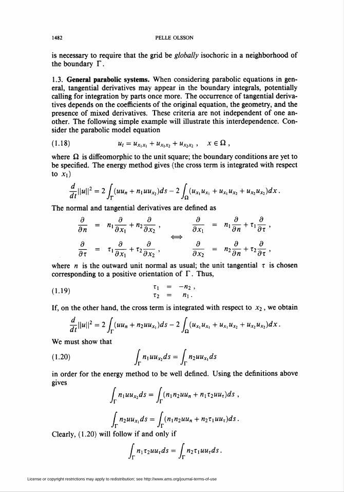
1482 PELLE OLSSON
is necessary to require that the grid be globally isochoric in a neighborhood of
the boundary Y.
1.3. General parabolic systems. When considering parabolic equations in gen-
eral, tangential derivatives may appear in the boundary integrals, potentially
calling for integration by parts once more. The occurrence of tangential deriva-
tives depends on the coefficients of the original equation, the geometry, and thepresence of mixed derivatives. These criteria are not independent of one an-other. The following simple example will illustrate this interdependence. Con-
sider the parabolic model equation
(1-18) ut = uXxM + uXxXl + uXlXl , x£Q,
where Q is diffeomorphic to the unit square; the boundary conditions are yet tobe specified. The energy method gives (the cross term is integrated with respect
to xx)
^||m||2 = 2 / (uu„ + nxuuX2)ds -2 (uX]uXi + uXtuX2 + uXluXl)dx.
The normal and tangential derivatives are defined as
d d d d d dd~n = nidx-x+n2dT2' dTx = nidH + Xldl'
d_ _d_ _d_ _d_ d_ d_dx " rldxx+r2dx2, dx2 ~ n2dn+X2dx'
where n is the outward unit normal as usual; the unit tangential x is chosen
corresponding to a positive orientation of Y. Thus,
(1.19) Tl _"2'
K J x2 = nx.
\u\\2 = 2 (uun + n2uuXi)ds -2 (uXiuXi + uXluX2 + uX2uXl)d)Jt Ja
If, on the other hand, the cross term is integrated with respect to x2 , we obtain
— Idv
We must show that
(1.20) / nxuuX2ds = / n2uuXids
in order for the energy method to be well defined. Using the definitions above
gives
/ nxuuX2ds = / (nxn2uun + nxx2uur)ds ,
/ n2uuXlds = ¡ (nxn2uu„ + n2xxuuT)ds.
Clearly, (1.20) will follow if and only if
/ nxx2uuxds = / n2xxuuxds .
License or copyright restrictions may apply to redistribution; see http://www.ams.org/journal-terms-of-use
SUMMATION BY PARTS, PROJECTIONS, AND STABILITY. II 1483
From (1.19) and n\ + n\=l it follows immediately that
/ nxx2uuxds — / n2xxuuxds - I uuxds .
Note that the second integral of the right-hand side would vanish identically
if T were smooth. To simplify the analysis, it will, as usual, be assumed that
u is supported only in a neighborhood of the lower left corner. Hence, it will
be sufficient to consider the boundary portions Ti and T4 corresponding to
£2 = 0 and ii = 0. Parameterizing Y in the positive direction gives (cf. (1.3))
/ uuxds = - -(u\dÇ2 + - (u\dÇx.
Letting £2 -> -£,2 in the first integral of the right member gives (d/dÇ2 ->
-d/dt2, dZ2-+dt2)
I uuxds = -l (u2)i2dÇ2 + 2 I (u\dtx = 0 ,
and (1.20) follows. The energy method is thus well defined, and we have
dtl\u\\2 < 2 / ((1 + nxn2)uu„ + n\uux)ds - (||«xill2 + ||Wx2||2)
The quantity n\ is discontinuous at the corners. Define the jump discontinuity
,2mv-\ _ „2 (v\ _ „2[nj](x) = n\R(x) - n2XL(x) ,
where n2R(x) and n2L(x) are the left and right limits of n2 at x (accordingto the positive orientation of Y). Straightforward computations show that
/ n\uuxds = 2 £["2]Oc,)w2Od, t) - 2 / (n\)xu2ds ,
where xci, i = 1, ... , 4, are the corner points. Thus,
4
— Idtl u\\2 <£[«2](^c,)«2 + / (2(1 + nxn2)uun - (n2)xu2j ds
;=i Jr
-(lKII2 + IIM2).
From this inequality it is obvious that giving Dirichlet data at the corners and
Neumann data at the remaining boundaries would yield an energy estimate.
In fact, we could even allow inhomogeneous Dirichlet data at the corners and
still obtain an energy estimate in terms of the data. The effect of the corners
disappears if and only if [«2](x) = 0, which happens if and only if
(i) «iz.0) = nXR(x) ,(ii) nXL(x) = -«i*0) .
The first case implies that the normal is continuous, i. e., x is not a corner point.The second case is more interesting, since the normal is discontinuous, but the
effect on the energy estimate disappears. This illustrates how the geometry can
interact with the cross terms. The simplest example is obtained by solving
License or copyright restrictions may apply to redistribution; see http://www.ams.org/journal-terms-of-use

1484 PELLE OLSSON
(1.18) on Ci being the square with (1,0), (0,1), (-1,0), and (0,-1) asvertices. Evidently, the second case holds at the corners, and no corner values
should appear in the energy estimate. This can also be seen by a change of
coordinates:
* = 7f1 + 7!X2'Í2 = -7=XX + j=X2.
Equation (1.18) is then transformed into
3 1 - . 1 1 , . 1 1 ,ut = -2uílíí + -2ut2i2, ^ (--,-),(--,-).
The cross term has vanished; instead the equation has become anisotropic. In
this coordinate system it is apparent that no tangential derivatives — and con-
sequently no point values — will appear when deriving the energy estimate.
To solve (1.18) by means of finite difference methods, it is rewritten in self-
adjoint form:
(1.21)
(j-xu)=±(j-x(i + ni%r)dc:k.du) +B-i)'(«iV1%Y .k=\ k kjil Ç*
where «^ = -dÇk/\dÇk\. This equation is discretized in space the usual way.
The cross terms
(-1)'(«<*>«<%)&
must be integrated twice to eliminate the tangential derivatives. In the semi-
discrete case this amounts to performing summation by parts twice, the second
of which will require the introduction of a commutator, thereby obliterating
strict stability (except for the second-order accurate difference operator). To
restore strict stability, it would be tempting to reformulate the critical terms in
skew-symmetric form:
«M% = \ KMS,+ ky'^< - 2" ("^V"Doing so, however, would introduce lower-order energy terms (•, •)„, whose
presence would destroy strict stability. The simplest way to resolve this am-biguity is to assume homogeneous Dirichlet data, in which case the boundary
terms vanish identically, and (1.21) would be the preferred choice. The choice
of homogeneous Dirichlet data to eliminate the influence of the mixed deriva-tives arises naturally when solving the Navier-Stokes equations, since at solid
boundaries we have zero velocity, and since the cross terms involve only the
velocity components.
License or copyright restrictions may apply to redistribution; see http://www.ams.org/journal-terms-of-use

SUMMATION BY PARTS, PROJECTIONS, AND STABILITY. II 1485
We now turn to general parabolic systems subject to homogeneous Dirichletconditions,
2
ut = Y, AUux,Xj + F , X £ Q ,
wO,0) = /O),«O,i) = 0, X£Y.
This equation can be rewritten in curvilinear coordinates as
(1.22)2 2
(•/"'M) = É (J~1^A'jUx) -E^toriAj^ + J^F, x£ü,' i,j,k=\ ^ ' '& 7=1
«O,0) = /O),u(x, /) = 0, x £ Y ,
where div(Aj) = (AXj)Xl + (A2J)X2. Define C¡ = div(^). The semidiscretesystem is then given by
(1.23)
(J~xv)t = P í ¿ DkJ-xMikAijDjV - ¿ J-lCjDjV + J~XF ) .
\i,j,k=\ 7=1 /
The projection operator P represents the homogeneous Dirichlet conditions.
Proposition 1.3. The approximation (1.23) is strictly stable.
Proof. Left to the reader, d
2. INHOMOGENEOUS BOUNDARY CONDITIONS
The principle for handling inhomogeneous boundary data is best illustratedby means of a simple example. Consider the one-dimensional advection equa-tion
(2.1)Ut + Ux = 0 , X £ (0, 1)
u(x,G) = f(x),u(0,t) = g(t).
The corresponding semidiscrete system reads
/0
(2.2) *t + PDvr(I-P)ët,' v(0) = f,
1
V 1/
g\
wwhere g}, j = 1, ... , v , are to be determined later. Obviously, vo(t) = g(t) if
fo = ¿?(0). The boundary condition is thus fulfilled at all time. More generally,
multiplying equation (2.2) by P (using P2 = P) and subtracting the resultingequation from (2.2), we can see that v = Pv + (I - P)g <*=> (/ - P)(v - g) - 0.
License or copyright restrictions may apply to redistribution; see http://www.ams.org/journal-terms-of-use
1486 PELLE OLSSON
Hence, the energy method gives
^\\v\\2h = -2(v-(I-P)g,Dv)h + 2(v,(I-P)gt)h.
Subtracting 2(g, vt)h from both sides, we get
2(v-g, v,)h = -2(v-g, Dv)h - 2(g, v, + PDv -(I- P)gt)h
+ 2(v-g,(I-P)gt)h.
Using (2.2) and (I - P)(v - g) = 0 shows that
2(v - g, vt)h =-2(v - g, Dv)h ,
i. e.,
2(v-g,(v- ~g)t)h = -2(v -g,D(v- g))h -2(v-g,gt + Dg)h.
If g solves the auxiliary problem
nX\ gt+Dg = 0,{¿-5) g(0) = f,
v-g\\l = -2(v -g,D(v- g))h = (vq - g)2 - (vv - gu)2 < 0
then
d_dt
since vq = g. Thus,
ll»(0-*(OIU<ll»(0)-*(0)|U--o
Consequently,
v(t) = g(t), t>0.
If g satisfies (2.3), we get the energy estimate
¿jïïgïïh = -2(g,D~g)h = g2- g2.
Hence,
\\g(t)\\2h+ f gl(r)dx = \\f\\2h+ f g2(x)dx.Jo Jo
Finally, v = g implies
\\v(t)\\2+ f v2(x)dx = \\f\\2+ [' g2(x)dx ,Jo Jo
which is identical to the continuous estimate.It remains to be verified under what circumstances g solves the auxiliary
problem (2.3). Let g = (go g\ ■■■ gv)T be the solution to (2.3). Hence,
DJg(0) = DJf, j = 0,l,...,
and
^7 + (-l)7+1ö^ = 0, í>0, 7 = 0,1,... ,
License or copyright restrictions may apply to redistribution; see http://www.ams.org/journal-terms-of-use

SUMMATION BY PARTS, PROJECTIONS, AND STABILITY. II 1487
i. e., for t = 0 we get the compatibility conditions
0(O) + (-ir1DV = O, ;=0,1,....
Thus, if we require that the initial-boundary data / and g satisfy
it follows that
^(0) + (-ir'(Z)V)o = 0, 7 = 0,1,
&0) = ^(0), 7 = 0,1,du du y
By virtue of being the solution to (2.3), go(t) is analytic in t. Hence, if the
boundary data g(t) is taken to be analytic, these equalities imply that g(t) =
go(t), t > 0, i.e., g = g, which proves that g indeed solves (2.3).
In what follows we shall analyze the general case. Consider the ODE system
nd) (J-xv)t = PR(t,v) + (I-P)(J-x~g)t ,[ ' v(0) = f,
with J~x being the inverse Jacobian, and where
R(t,v) = G(t,v) + J~xF(t) , G(t,0) = 0.
This form arises naturally when discretizing a nonlinear PDE in space; g rep-
resents the boundary data, and F is the forcing function; G(t,v) is the dis-cretization of the differential operator. It should be pointed out that most op-
erators G occurring in practice are autonomous, i. e., G = G(v). We usethe tilde notation to emphasize that g is only partially determined, that is,
some components are determined by the boundary data of the underlying PDE;the remaining components are unknown. It is no restriction to assume thatg = (¿?o • • • gv )T with gi, i = 0, ... , s, being the known components; s
is of course independent of the meshsize. Otherwise, g could be brought to
this form by permuting the dependent variables appropriately. As usual, werequire that P and J~x commute, which is true if the grid is locally isochoric
at the boundary. Next, we define the auxiliary problem
(J-xw)t = R(t,w),
[ ' w(0) = f.
Any solution to (2.5) will satisfy
^-(j-xw)=Rj(t,w), 7 = 0,1,...,
where Rj is defined recursively by
Rj(t,w) = ^^(t,w) + ^^-(t,w)JR(t,w), 7=1,2,... ,
R0(t, w) = J~xw.
Consequently, at t - 0 we have
£j(j-lw)(0) = Rj(0,f), 7 = 0,1,....
License or copyright restrictions may apply to redistribution; see http://www.ams.org/journal-terms-of-use
1488 PELLE OLSSON
Assumption 2.1. The boundary data g¡(t), i = 0, ... , s, the initial data /,
and the forcing function F satisfy the compatibility conditions
^j(j-lg).(0) = (Rj(0,f))i , i = 0,...,s, 7 = 0,1,....
If R is sufficiently well behaved, in particular if G is linear and autonomous,
then w(t) will be analytic for 0 < t < T. Thus, if we require that the boundary
data gi(t), i = 0,... , s, be analytic, it follows that
gi(t) = Wj(t) , i = 0, ... ,s.
Furthermore, the unknown components g¡, i > s, are of course taken to be
gi(t) = Wi(t), i>s.
Hence, g = w solves (2.5).
Remark. It suffices to consider g¡ piecewise analytic, since the process can be
repeated at t = tx, where tx is the critical time when analyticity is lost.
Proposition 2.1. Let v be the solution to (2.4) and suppose that Assumption 2.1
holds. If the boundary data g¡(t), i = 0, ... , s, are piecewise analytic in t,
then
(v-g,(v- ~g)t)h = (v-g,G(t,v)- G(t, g))h.
Proof. Using (2.4) and Pv — v - (I - P)g, which is true since P and J~x
commute, we readily conclude that
(v, vt)h = (v-g,R(t, v))h + (g, PR(t, v))h + (v,(I- P)(J-lg),)h .
Hence,
{v-g, vt)h = (v-g,R(t, v))h + (g, -(J~lv), + PR(t, v))h
+ (v,(I-P)(J-xg)t)h,
or, using (2.4),
(v-g, vt)n = (v-g,R(t, v))h + (v-g,(I- P)(J-lg)t)h .
But
(v-g, (I- P)(J-xg)t)h = ((/ - P)(v - g), (J-Xg)t)h = 0 ,
and so
(v-g,v,)h = (v -g,R(t,v))h ,
which in turn is equivalent to
(v-g,(v- g)t)h = (v-g,R(t,v)- R(t, g))h -(v-g, (J~l~g)t - R(t, g))h .
The assumptions on g imply that (J~xg)t = R(t, g), which proves the propo-
sition. □
License or copyright restrictions may apply to redistribution; see http://www.ams.org/journal-terms-of-use
SUMMATION BY PARTS, PROJECTIONS, AND STABILITY. II 1489
2.1. One-dimensional parabolic systems. We consider the parabolic system
(lower-order terms are omitted for convenience)
ut = (Aux)x + F ,
(2.6) u(x,0) = f,L0u(0, t) + Lxux(0, t) = g(t) ,
where
-$)■ = m. *«> = «"and u £ Rd , rank(L() = dx, rank(L'0') = d2, dx + d2 = d. Equation (2.6) isassumed to be strongly parabolic, i. e., there exists a constant ô > 0 such that
uTA(x, t)u > 2ô\u\2. Furthermore, A(x, t) is assumed to satisfy the following
compatibility condition [1, Lemma 7. 2. 1, p. 215]: For a, b £ Rd satisfying
Ltfa = 0, L[b = 0, one has aTA(0, t)b = 0. The boundary data g(t) isassumed to be piecewise analytic in t.
Let the boundary projection P be given by (1.8); the discretized analytic
boundary conditions are defined by LTv = L0v0 + Lx(Dv)0 = g(t). The hy-
potheses for Ln, Li and the compatibility condition on A imply that L has
full rank if the mesh size h is small enough [2, §3. 2]. Hence, there exists a vec-
tor g(t) £ R^+X^d such that g(t) = LTg(t), i. e., LTv = g *=> LT(v -g) = 0.
The semidiscrete approximation of (2.6) can then be formulated as
nT. vt = P(DADv + F) + (I-P)g,,[J) v(0) = f.
Assuming that initial data satisfy LTf = g, we have that (multiply (2.7) by
P and subtract the result from (2.7)) (/ - P)(v - g) = 0 or, equivalently,
LTv = LTg. Thus,
L0v0 + Lx(Dv)o = g ,
which shows that the analytic boundary conditions are satisfied to some order
of accuracy.
Proposition 2.2. // in addition to the previous hypotheses, Assumption 2.1 holds,
then (2.7) is strictly stable.
Proof. We know that g solves the auxiliary problem
gt = G(t,g) + F(t),
g(0) = f,
where G(t, g) = DAD g . Proposition 2.1 then yields (using J = I)
(v-g,(v- g)t)h = (v-g, DAD(v - g))h
< -(vo - go)TA(D(v - g))0 - 2S\\D(v - g)\\l ■
Since LT(v - g) = 0, it follows that
L''(vo-go) = 0.
Furthermore, decompose Vj - g¡ = (v'j - g'j) + (v'J - g"), where v'j, g'j £
ker(L{), v'J, g'j £ ker(L{)-L. According to the compatibility condition on A
License or copyright restrictions may apply to redistribution; see http://www.ams.org/journal-terms-of-use
1490 PELLE OLSSON
we then obtain
(v-g,(v- g)t)h < -(vo - go)TA(D(v" - g"))o - 2S\\D(v - g)\\l ■
Arguing exactly as in the proof of the homogeneous case [2, proof of Proposition
3. 2] gives
(D(v"-g"))o = -L7lLo(v0-go),
where
Lx =si
\'&
{Sj} is a basis in kerL{, whence Li is invertible. Consequently,
(v-g,(v- g)t)h < y\v0 - go\2 - 2ô\\D(v - g)\\\ ■
By means of the discrete Sobolev inequality we thus arrive at
(v-g,(v- g)t)h < (| + cf(h)) \\v - g\ |22 .-vv;,,- .,U-
Thus,
ll«(0 - g(t)\\h < eW<h»'\\v(0) - g(0)\\h = 0 ,
which is equivalent to v(t) = g(t), t > 0.
To get the final estimate, we consider the auxiliary problem. One obtains
£-\\g\\2 < -2g^A(Dg")o - 4ô\\Dg\\2 + HUI2 + II^H2 .
Now
L0g0 + Lx(Dg")o = g ,
and so
(JDr)o = -Lrl^o^o + ¿r1^-
Thus,
-2gTA(Dg")o = 2gT¡AL-xLogo - 2g0TAL7lg < y\g0\2 + \g\2 ,
where the algebraic inequality 2xy <cx2 + c~xy2 was used. This leads to
¿¿Muí + \go\2 <(7+ l)\go\2 - 4ô\\Dg\\2 + \\g\\2 + \g\2 + \\F\\2.
The coefficients of this estimate are exactly the same as those of the correspond-
ing analytic inequality. Using g = v and eliminating the boundary terms of
the right member by means of the Sobolev inequality yields
^|M|2 + \v0\2 < (a + cf(h))\\v\\2 + \g\2 + \\F\\2,
where a is the same constant as in the analytic estimate. Finally, integration
with respect to time results in
\\v\\l + f \v0(r)\2dx < e^h»< (||/||2 + jf (\g(x)\2 + \\F(x)\\2) dx} ,
which is the desired estimate. □
License or copyright restrictions may apply to redistribution; see http://www.ams.org/journal-terms-of-use
SUMMATION BY PARTS, PROJECTIONS, AND STABILITY. II 1491
Remark. The boundary conditions are used twice — first in conjunction with
Proposition 2.1 to show that g = v , and second with the auxiliary problem to
get the actual estimate. It should be emphasized that the hypotheses preced-
ing the formulation of Proposition 2.2 are needed in order to prove an energy
estimate for the analytic problem (2.6). We do not claim that the additional
assumption in the previous proposition is necessary.
2.2. Two-dimensional symmetric hyperbolic systems. We consider equation
(1.12) with the lower-order terms omitted for convenience. The boundary con-
ditions are given by L(x)u(x, t) - g(x, t), x £Y, where the analytic boundary
operator L(x) is identical to that of §1.1. The discrete boundary operator isdefined as
(LTv)ij = g(Xij, t) , i' = 0,i/, j = 1,... , v - 1 , and
7' = 0, ,, , i = 0, ... ,u ,
or, in global form,
LTv = g.
Since L has full rank, it follows that there exists a vector g(t) such that LTg =g. Thus,
LT(v-g) = 0.
Equation (1.12) is discretized as
(2.8)
(j~Xv)t = P U Y (DíJ-xBíV + J-xBiDiv) + J-xf\ +(I-P) (J-Xg)t,
v(0) = f,
where P is the orthogonal projection corresponding to the global operator LT.
Proposition 2.3. Suppose that Assumption 2.1 holds. Then (2.8) is strictly stable.
Proof. By Assumption 2.1, g solves the auxiliary problem
(j-lg)t = G(t,g) + J-xF(t),
where
, 2G(t> 8) = 2 E {DiJ~lB>8 + J-'BiDig) .
i=i
Hence, according to Proposition 2.1 we have
. 2
(V -g, (V - g)t)h = -Y(v-g, [DíJ-'Bí + J-'BíDÍ) (v - g))n.i=i
Summation by parts yields
(v - g, (v - g)t)h = -(v-g, (nxAx + n2A2) (v - g))r.
License or copyright restrictions may apply to redistribution; see http://www.ams.org/journal-terms-of-use
1492 PELLE OLSSON
But LT(v - g) = 0, whence v-g satisfies the homogeneous boundary condi-
tions. Consequently (cf. the proof of Proposition 1.1),
(v-g, (nxAx+n2A2)(v-g))r< ~y\v - g\l < 0.
Thus, g(t) = v(t), t>0.In the second part of the proof we apply the energy method to the auxiliary
problem. Straightforward computations show that
¿j(è > ê)h = (g. (Mi + n2A2) ¿?>r + 2(g, F)h .
Take an arbitrary point x0j on the boundary portion where £1 = 0. We must
analyze the quadratic form
gl{n^Ax + n^A2)^j
We know that LTg = g, where g is the vector representing the analytic bound-
ary data. Define tpij = QT(x¡j)gij . Hence,
(2.9) (fu)t = S(xu)((pij)II + gu ,
and the quadratic form is transformed into
ëoj (n[X)Ax + n{2l)A2} g0j = 9ojMj<Poj ■
Using (2.9) gives (omitting the spatial subscripts for simplicity)
tpTAtp = tpj¡ (A// + STAjS) <pu + 2(pJ,STA,g + gTA¡g.
It is assumed that A¡¡ < -y at x0;. For sufficiently small S we thus get
,»7Af<-j[|fzj|2 + (l + |Aj|)|*|2.
Now, \tpi\ < \S\\(pn\ + \g\. Hence,
tpTAtp + y-\<p\2 < -J^l2 + y-\<pj\2 + (1 + |A/|) \g\2 <(3 + |A/|) \g\2
for S small enough. It should be underscored that this is exactly the same
estimate one gets in the continuous case. At each boundary point xoj we have
thus established that
êïj (n[x)Ax + n2X)A2)Q. g0j + 7-f\g0j\2 < (3 + \(A0j),\) \g0j\
with a similar expression at points x,o corresponding to ¿,2 = 0. Letting
inf(y¡j) = y > 0, we thus obtain
jt(g,g)h + \(g,g)r<0 + \^U(g,g)v + 2(~g,F)h.
License or copyright restrictions may apply to redistribution; see http://www.ams.org/journal-terms-of-use
SUMMATION BY PARTS, PROJECTIONS, AND STABILITY. II 1493
Finally, with the identification v = g, integration gives the energy estimate
(v(t),v(t))h+ I (v(x),v(x))TdxJo
< Ke> ((/, f)h + jf ((g(x), g(x))T + (F(x), F(x))h)dx} ,
which proves the theorem. □
Remark. Because of the terms (pJ,STA¡g + gTA¡g, the constant K of the en-
ergy estimate will in general satisfy K > 1, even if no estimate of the boundary
terms (v , v)r is wanted. For g = 0, i. e., homogeneous boundary conditions,
the critical terms disappear, and one may take K = 1 in case no boundary
estimate is needed.
Bibliography
1. Heinz-Otto Kreiss and Jens Lorenz, Initial-boundary value problems and the Navier-Stokes
equations, Pure and Applied Mathematics, vol. 136, Academic Press, San Diego, CA, 1989.
2. Pelle Olsson, Summation by parts, projections, and stability. I, Math. Comp. 64 (1995), 1035—1065.
RIACS, Mail Stop T20G-5, NASA Ames Research Center, Moffett Field, California94035-1000
E-mail address: pelleQriacs.edu
License or copyright restrictions may apply to redistribution; see http://www.ams.org/journal-terms-of-use