Summary Weeks 1-6

8/6/2019 Summary Weeks 1-6

http://slidepdf.com/reader/full/summary-weeks-1-6 1/24

What we have covered in MEDI1013 weeks 1 to 6. This covers some additional

material together with some answers for the tutorial questions. Hope it is useful.

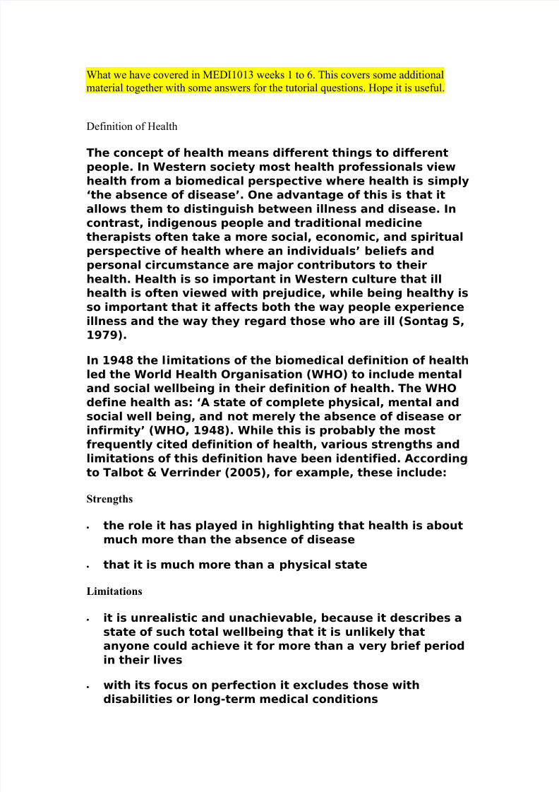
Definition of Health

The concept of health means different things to different

people. In Western society most health professionals view

health from a biomedical perspective where health is simply

‘the absence of disease’. One advantage of this is that it

allows them to distinguish between illness and disease. In

contrast, indigenous people and traditional medicine

therapists often take a more social, economic, and spiritual

perspective of health where an individuals’ beliefs and

personal circumstance are major contributors to their

health. Health is so important in Western culture that illhealth is often viewed with prejudice, while being healthy is

so important that it affects both the way people experience

illness and the way they regard those who are ill (Sontag S,

1979).

In 1948 the limitations of the biomedical definition of health

led the World Health Organisation (WHO) to include mental

and social wellbeing in their definition of health. The WHO

define health as: ‘A state of complete physical, mental and

social well being, and not merely the absence of disease orinfirmity’ (WHO, 1948). While this is probably the most

frequently cited definition of health, various strengths and

limitations of this definition have been identified. According

to Talbot & Verrinder (2005), for example, these include:

Strengths

• the role it has played in highlighting that health is about

much more than the absence of disease

• that it is much more than a physical state

Limitations

• it is unrealistic and unachievable, because it describes a

state of such total wellbeing that it is unlikely that

anyone could achieve it for more than a very brief period

in their lives

• with its focus on perfection it excludes those with

disabilities or long-term medical conditions



• its lack of inclusion of spiritual wellbeing

• its definition of individual health out of a cultural and

ecological context

• it is unmeasurable (statistics still only enable us tomeasure death and disease)



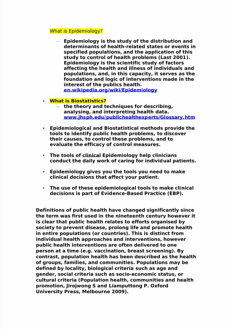
What is Epidemiology?

– Epidemiology is the study of the distribution anddeterminants of health-related states or events inspecified populations, and the application of this

study to control of health problems (Last 2001).Epidemiology is the scientific study of factorsaffecting the health and illness of individuals andpopulations, and, in this capacity, it serves as thefoundation and logic of interventions made in theinterest of the publics health.en.wikipedia.org/wiki/Epidemiology

• What is Biostatistics? – the theory and techniques for describing,

analysing, and interpreting health data.www.jhsph.edu/publichealthexperts/Glossary.ht m

• Epidemiological and Biostatistical methods provide thetools to identify public health problems, to discovertheir causes, to control these problems, and toevaluate the efficacy of control measures.

• The tools of clinical Epidemiology help cliniciansconduct the daily work of caring for individual patients.

• Epidemiology gives you the tools you need to makeclinical decisions that affect your patient.

• The use of these epidemiological tools to make clinicaldecisions is part of Evidence-Based Practice (EBP).

Definitions of public health have changed significantly since

the term was first used in the nineteenth century however it

is clear that public health relates to efforts organised by

society to prevent disease, prolong life and promote health

in entire populations (or countries). This is distinct from

individual health approaches and interventions, however

public health interventions are often delivered to one

person at a time (e.g. vaccination, breast screening). By

contrast, population health has been described as the health

of groups, families, and communities. Populations may be

defined by locality, biological criteria such as age and

gender, social criteria such as socio-economic status, or

cultural criteria (Population health, communities and health

promotion, Jirojwong S and Liamputtong P. OxfordUniversity Press, Melbourne 2009).

http://www.google.com.au/url?sa=X&start=26&oi=define&q=http://en.wikipedia.org/wiki/Epidemiology&usg=__VsnAP51WHXvyes125bJspUV37l0=

http://www.google.com.au/url?sa=X&start=0&oi=define&q=http://www.jhsph.edu/publichealthexperts/Glossary.htm&usg=__FT-IPRutiTtimEZnEDuoHrq-_jc=

http://www.google.com.au/url?sa=X&start=26&oi=define&q=http://en.wikipedia.org/wiki/Epidemiology&usg=__VsnAP51WHXvyes125bJspUV37l0=





Public health has been described as having three domains:

health improvement (or promotion), health protection and

health social care quality.

Health improvement uses a combination of health education

and population interventions, such as anti-smokingcampaigns to facilitate behavioural and environmental

changes conducive to health enhancement and harm

reduction (Population health, communities and health

promotion, Jirojwong S and Liamputtong P. Oxford

University Press 2009).

Health protection is concerned with immediate threats to

health such as infectious diseases and environmental

threats, e.g. chemical hazards, natural disasters and

terrorism.

Health social care quality is concerned with using evidence-

based methods to develop efficient health system policies,

quality standards and evaluation practices.

Evidence-based practice (EBP)• Defined as “the conscientious, judicious and explicit

use of current best evidence in making decisions aboutthe care of the individual patient (Sackett DL et al.,2000).

• Compliments clinical expertise in the provision of bestpatient care.

EBP consists of five steps steps• Frame the clinical question (be specific)

• Search the evidence – Much of this evidence has been obtained using

epidemiological methods

• Appraise the evidence (critical appraisal) – Using epidemiological & biostatistical tools

• Apply the evidence

• Evaluate the application of the evidence.



• Incidence versus prevalence

Incidence refers to the frequency of development of a new illness in a

population in a certain period of time, normally one year. When we say that the

incidence of this cancer has increased in past years, we mean that more people

have developed this condition year after year, i.e.:, the incidence of thyroid

cancer has been rising, with 13,000 new cases diagnosed this year.

Prevalence refers to the current number of people suffering from an illness in a

given year. This number includes all those who may have been diagnosed in prior

years, as well as in the current year. The incidence of a cancer is 20,000 year

with a prevalence of 80,000 means that there are 20,000 new cases diagnosed

every year and there are 80,000 people living in the United states with this

illness, 60,000 of whom were diagnosed in the past decade and are still living

with the disease. The number of people cured of the disease is not included in

prevalence.

Point vs. Period Prevalence

The amount of disease present in a population obviously changes over time.

Sometimes, we want to know how much of a particular disease is present in a

population at a single point in time, a sort of snapshot view.

• Point Prevalence: For example, we may want to find out the prevalence of

TB in Community A today. To do that, we need to calculate the point

prevalence on a given date.

– The numerator would include all known TB patients who live in

Community A that day. That information could be determined from a

TB case registry.

– The denominator would be the population of Community A that day.

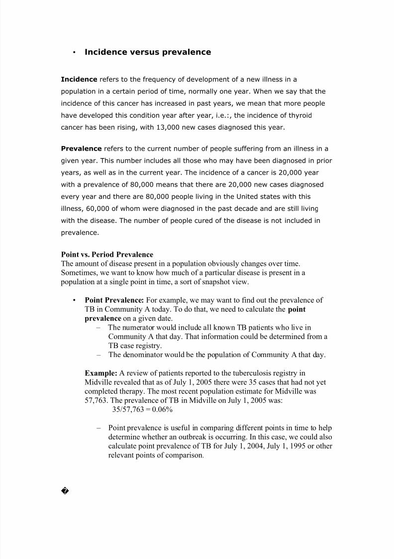
Example: A review of patients reported to the tuberculosis registry in

Midville revealed that as of July 1, 2005 there were 35 cases that had not yet

completed therapy. The most recent population estimate for Midville was57,763. The prevalence of TB in Midville on July 1, 2005 was:

35/57,763 = 0.06%

– Point prevalence is useful in comparing different points in time to help

determine whether an outbreak is occurring. In this case, we could also

calculate point prevalence of TB for July 1, 2004, July 1, 1995 or other

relevant points of comparison.

�



The classic descriptors of how common a disease, symptom, or problem is ina population are incidence and prevalence.

Incidence quantifies the number of new problems that develop in a

population at risk during a given period of time (for example, new symptomssuch as new instances of breathlessness). Incidence is quantified as a RATE:

incidence=number of new problems during a given period of time

total population (or person-time) at risk

Incidence provides an estimate of the probability (or risk) that a patient willdevelop the problem during the given period of time.

For example: At admission, 120 patients free from breathlessness arefollowed for 3 weeks. In this period of time, 45 developed breathlessness.

This results in a incidence rate of 45 per 120 (or 37.5 %) during the 3 weekperiod. This means that, at admission, each patient had a .375 probability todevelop breathlessness during the next 3 weeks.

Prevalence quantifies the proportion of a given population with a problem (for example, breathlessness) at a designated time. When the term is usedwithout qualification of a time period it is usually the point prevalence, for example the proportion of patients with breathlessness at a given point intime. Note that, although the term "prevalence rate" is used for prevalence,prevalence is a proportion, not a rate.

prevalence= number of patients with the problem

at a designed timetotal population

For example: At admission, 150 patients were screened for the presence of breathlessness, and 30 resulted affected by the symptom. This results in abreathlessness prevalence at admission of 20% (30/150).

The period prevalence refers to the proportion of a given population with aproblem (for example, breathlessness) at any time during a specified period.Period prevalence can refer to proportion with the problem at any time in one

year (annual prevalence) or at any time in their life (lifetime prevalence).

�

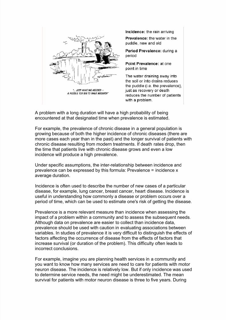
Incidence and prevalence are closely related. Prevalence (the proportion of apopulation with a problem at a designated time) depends on both theincidence (the rate of new problem during a period of time) and the duration of the problem as is illustrated by the following cartoon.

Figure 4.1: Illustration of Incidence and Prevalence



A problem with a long duration will have a high probability of beingencountered at that designated time when prevalence is estimated.

For example, the prevalence of chronic disease in a general population isgrowing because of both the higher incidence of chronic diseases (there aremore cases each year than in the past) and the longer survival of patients withchronic disease resulting from modern treatments. If death rates drop, thenthe time that patients live with chronic disease grows and even a lowincidence will produce a high prevalence.

Under specific assumptions, the inter-relationship between incidence andprevalence can be expressed by this formula: Prevalence = incidence xaverage duration.

Incidence is often used to describe the number of new cases of a particular disease, for example, lung cancer, breast cancer, heart disease. Incidence isuseful in understanding how commonly a disease or problem occurs over aperiod of time, which can be used to estimate one's risk of getting the disease.

Prevalence is a more relevant measure than incidence when assessing theimpact of a problem within a community and to assess the subsequent needs.

Although data on prevalence are easier to collect than incidence data,prevalence should be used with caution in evaluating associations betweenvariables. In studies of prevalence it is very difficult to distinguish the effects of factors affecting the occurrence of disease from the effects of factors thatincrease survival (or duration of the problem). This difficulty often leads toincorrect conclusions.

For example, imagine you are planning health services in a community andyou want to know how many services are need to care for patients with motor neuron disease. The incidence is relatively low. But if only incidence was usedto determine service needs, the need might be underestimated. The mean

survival for patients with motor neuron disease is three to five years. During



many of these years patients experience increasing symptoms and problems.Thus prevalence is more useful to assess the need for services.

Definition of a case:

Measuring symptom frequency in populations requires the stipulation of diagnostic criteria. In clinical practice the definition of a "case" generallyassumes that, for any symptom, people are divided into two discrete classes:the affected and the un-affected.

To define who has a symptom it is important to use a valid and reliablemethod of assessment. This can be a problem in palliative care where studieshave found only a modest correlation between symptom assessment bypatients and symptom assessment by clinicians. The same modest correlationin symptom assessment has been found between patients and families. In

addition, patients who are very weak or ill may not be well enough to reportsymptoms or their reports may be affected by cognitive impairment.

Two further complexities exist when assessing symptoms:

• Symptoms are often not dichotomized into present and absent.Symptoms are present in a spectrum of severity from none tooverwhelming;

• Assessment methods involve issues such as who gives theinformation? Is it assessed retrospectively or prospectively? whatquestion is asked? And do patients respond describing the treatedsymptom, or its effect on them? For example, when bereaved familymembers say that the patient had pain in the last year of life, are theysaying that the patient had pain, that was treated and was controlled,or did they have pain that wasn't treated? Some patients respond to thequestion "Do you have pain?" with "Yes, I am taking a high dose of morphine for my pain."

When describing or comparing symptom prevalence and incidence, the

results can be affected by such factors as:

• Time (for example time of day, time period included); • Place (for example, home, hospital, open plan hospital ward or in a

private room, out-patient clinic); and

• Person (this includes both the sociodemographic and clinicalcircumstances of the patient, for example, age, stage of disease, andthe person who collects the data).



Types of Study Design

The two main classes of study design are experimental and non-experimental.In an experimental study, conditions (usually the treatments) are under the

direct control of the investigator. These studies test the effectiveness of atreatment or intervention by comparing the outcome (for example thefrequency and intensity of a symptom) in the experimental group with theoutcome in the control group. In a randomized controlled trial, individuals arerandomly allocated to the groups.

Non-experimental studies observe something that naturally occurs.Descriptive studies describe patterns of disease, symptoms, or problems in apopulation. Analytic studies examine an association between a problem of interest and other variables, and possible causative factors are examined.These last groups include cross-sectional, longitudinal, and case-control

designs.

Symptoms can be studied in both experimental and non-experimental studies.The principles of detecting, measuring, and recording symptoms are shared inall these designs. The remainder of this chapter focuses on two common non-experimental designs used in symptom studies: cross-sectional andlongitudinal.

� Cross Sectional Study

A cross-sectional study (also called a prevalence survey) measures theprevalence of a symptom, determinants of a symptom, or both, in a populationat one point in time or over a short period of time. It provides a snapshot of the health experience of a population at a given time. Such information can bevery useful in assessing the health status and needs of a population. It canalso be used to study the relationship between variables (for examplebetween breathlessness and lung metastasis). The prevalence of a problem,rather than the incidence, is recorded in a cross-sectional survey, and everyassociation should be interpreted cautiously. Bias may arise because of selection into or out of the study population. For example, in a hospital survey,patients staying for a shorter period in hospital have less probability of being

included in a cross-sectional survey.

Cohort Studies

�

In a longitudinal study subjects are followed over time typically with repeatedmonitoring of symptoms or other variables. Such studies can vary enormously

in their size and complexity. At one extreme symptoms could be studiedrepeatedly in a large group (or cohort) of patients, from diagnosis to death. At



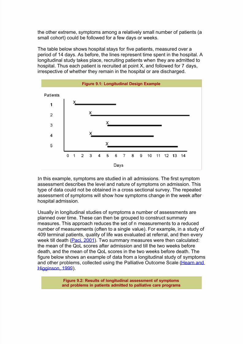
the other extreme, symptoms among a relatively small number of patients (asmall cohort) could be followed for a few days or weeks.

The table below shows hospital stays for five patients, measured over aperiod of 14 days. As before, the lines represent time spent in the hospital. A

longitudinal study takes place, recruiting patients when they are admitted tohospital. Thus each patient is recruited at point X, and followed for 7 days,irrespective of whether they remain in the hospital or are discharged.

Figure 9.1: Longitudinal Design Example

In this example, symptoms are studied in all admissions. The first symptomassessment describes the level and nature of symptoms on admission. Thistype of data could not be obtained in a cross sectional survey. The repeatedassessment of symptoms will show how symptoms change in the week after hospital admission.

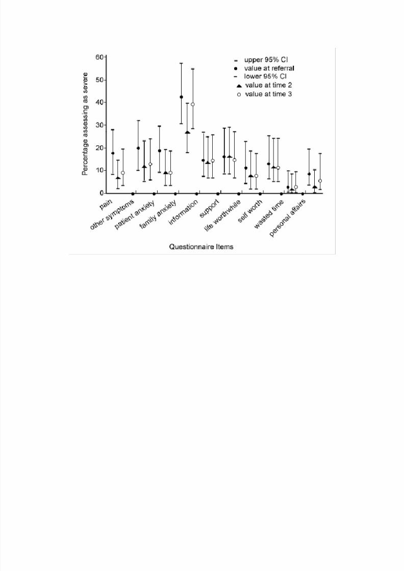
Usually in longitudinal studies of symptoms a number of assessments areplanned over time. These can then be grouped to construct summarymeasures. This approach reduces the set of n measurements to a reducednumber of measurements (often to a single value). For example, in a study of 409 terminal patients, quality of life was evaluated at referral, and then every

week till death (Paci, 2001). Two summary measures were then calculated:the mean of the QoL scores after admission and till the two weeks beforedeath, and the mean of the QoL scores in the two weeks before death. Thefigure below shows an example of data from a longitudinal study of symptomsand other problems, collected using the Palliative Outcome Scale (Hearn andHigginson, 1999).

Figure 9.2: Results of longitudinal assessment of symptomsand problems in patients admitted to palliative care programs

http://www.ncbi.nlm.nih.gov/entrez/query.fcgi?cmd=Retrieve&db=PubMed&list_uids=11239736&dopt=Abstract










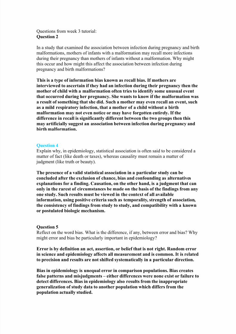
Questions from week 3 tutorial:

Question 2

In a study that examined the association between infection during pregnancy and birth

malformations, mothers of infants with a malformation may recall more infections

during their pregnancy than mothers of infants without a malformation. Why mightthis occur and how might this affect the association between infection during

pregnancy and birth malformations?

This is a type of information bias known as recall bias. If mothers are

interviewed to ascertain if they had an infection during their pregnancy then the

mother of child with a malformation often tries to identify some unusual event

that occurred during her pregnancy. She wants to know if the malformation was

a result of something that she did. Such a mother may even recall an event, such

as a mild respiratory infection, that a mother of a child without a birth

malformation may not even notice or may have forgotten entirely. If the

difference in recall is significantly different between the two groups then thismay artificially suggest an association between infection during pregnancy and

birth malformation.

Question 4

Explain why, in epidemiology, statistical association is often said to be considered a

matter of fact (like death or taxes), whereas causality must remain a matter of

judgment (like truth or beauty).

The presence of a valid statistical association in a particular study can be

concluded after the exclusion of chance, bias and confounding as alternatives

explanations for a finding. Causation, on the other hand, is a judgment that can

only in the rarest of circumstances be made on the basis of the findings from any

one study. Such results must be viewed in the context of all available

information, using positive criteria such as temporality, strength of association,

the consistency of findings from study to study, and compatibility with a known

or postulated biologic mechanism.

Question 5

Reflect on the word bias. What is the difference, if any, between error and bias? Whymight error and bias be particularly important in epidemiology?

Error is by definition an act, assertion, or belief that is not right. Random error

in science and epidemiology affects all measurement and is common. It is related

to precision and results are not shifted systematically in a particular direction.

Bias in epidemiology is unequal error in comparison populations. Bias creates

false patterns and misjudgments – either differences were none exist or failure to

detect differences. Bias in epidemiology also results from the inappropriate

generalization of study data to another population which differs from the

population actually studied.





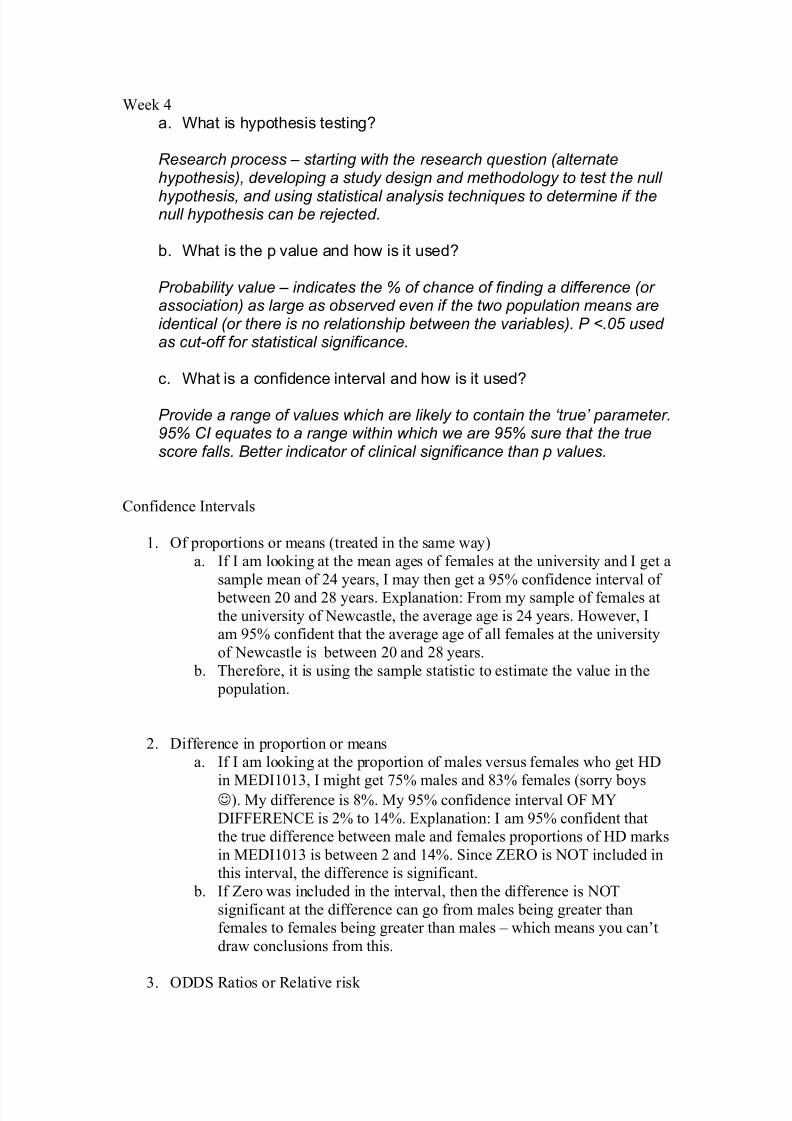
Week 4

a. What is hypothesis testing?

Research process – starting with the research question (alternatehypothesis), developing a study design and methodology to test the null

hypothesis, and using statistical analysis techniques to determine if thenull hypothesis can be rejected.

b. What is the p value and how is it used?

Probability value – indicates the % of chance of finding a difference (or association) as large as observed even if the two population means areidentical (or there is no relationship between the variables). P <.05 used as cut-off for statistical significance.

c. What is a confidence interval and how is it used?

Provide a range of values which are likely to contain the ‘true’ parameter.95% CI equates to a range within which we are 95% sure that the truescore falls. Better indicator of clinical significance than p values.

Confidence Intervals

1. Of proportions or means (treated in the same way)

a. If I am looking at the mean ages of females at the university and I get a

sample mean of 24 years, I may then get a 95% confidence interval of

between 20 and 28 years. Explanation: From my sample of females at

the university of Newcastle, the average age is 24 years. However, I

am 95% confident that the average age of all females at the university

of Newcastle is between 20 and 28 years.

b. Therefore, it is using the sample statistic to estimate the value in the

population.

2. Difference in proportion or means

a. If I am looking at the proportion of males versus females who get HD

in MEDI1013, I might get 75% males and 83% females (sorry boys). My difference is 8%. My 95% confidence interval OF MY

DIFFERENCE is 2% to 14%. Explanation: I am 95% confident that

the true difference between male and females proportions of HD marks

in MEDI1013 is between 2 and 14%. Since ZERO is NOT included in

this interval, the difference is significant.

b. If Zero was included in the interval, then the difference is NOT

significant at the difference can go from males being greater than

females to females being greater than males – which means you can’t

draw conclusions from this.

3. ODDS Ratios or Relative risk



a. If 1 is included in either of the confidence intervals, it means that the

OR or the RR could potentially be 1 which means that there is no

relationship or difference between the risks or odds of either group.

Therefore, if your OR or RR is significant, the confidence interval

MUST NOT contain 1.



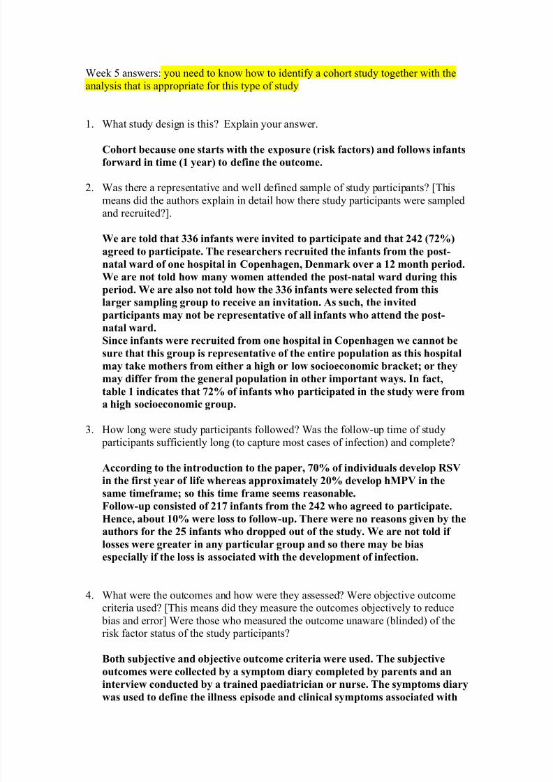
Week 5 answers: you need to know how to identify a cohort study together with the

analysis that is appropriate for this type of study

1. What study design is this? Explain your answer.

Cohort because one starts with the exposure (risk factors) and follows infants

forward in time (1 year) to define the outcome.

2. Was there a representative and well defined sample of study participants? [This

means did the authors explain in detail how there study participants were sampled

and recruited?].

We are told that 336 infants were invited to participate and that 242 (72%)

agreed to participate. The researchers recruited the infants from the post-

natal ward of one hospital in Copenhagen, Denmark over a 12 month period.

We are not told how many women attended the post-natal ward during thisperiod. We are also not told how the 336 infants were selected from this

larger sampling group to receive an invitation. As such, the invited

participants may not be representative of all infants who attend the post-

natal ward.

Since infants were recruited from one hospital in Copenhagen we cannot be

sure that this group is representative of the entire population as this hospital

may take mothers from either a high or low socioeconomic bracket; or they

may differ from the general population in other important ways. In fact,

table 1 indicates that 72% of infants who participated in the study were from

a high socioeconomic group.

3. How long were study participants followed? Was the follow-up time of study

participants sufficiently long (to capture most cases of infection) and complete?

According to the introduction to the paper, 70% of individuals develop RSV

in the first year of life whereas approximately 20% develop hMPV in the

same timeframe; so this time frame seems reasonable.

Follow-up consisted of 217 infants from the 242 who agreed to participate.

Hence, about 10% were loss to follow-up. There were no reasons given by the

authors for the 25 infants who dropped out of the study. We are not told if

losses were greater in any particular group and so there may be biasespecially if the loss is associated with the development of infection.

4. What were the outcomes and how were they assessed? Were objective outcome

criteria used? [This means did they measure the outcomes objectively to reduce

bias and error] Were those who measured the outcome unaware (blinded) of the

risk factor status of the study participants?

Both subjective and objective outcome criteria were used. The subjective

outcomes were collected by a symptom diary completed by parents and an

interview conducted by a trained paediatrician or nurse. The symptoms diarywas used to define the illness episode and clinical symptoms associated with



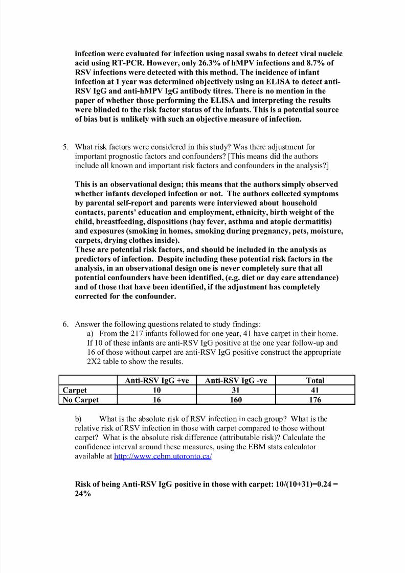
infection were evaluated for infection using nasal swabs to detect viral nucleic

acid using RT-PCR. However, only 26.3% of hMPV infections and 8.7% of

RSV infections were detected with this method. The incidence of infant

infection at 1 year was determined objectively using an ELISA to detect anti-

RSV IgG and anti-hMPV IgG antibody titres. There is no mention in the

paper of whether those performing the ELISA and interpreting the resultswere blinded to the risk factor status of the infants. This is a potential source

of bias but is unlikely with such an objective measure of infection.

5. What risk factors were considered in this study? Was there adjustment for

important prognostic factors and confounders? [This means did the authors

include all known and important risk factors and confounders in the analysis?]

This is an observational design; this means that the authors simply observed

whether infants developed infection or not. The authors collected symptoms

by parental self-report and parents were interviewed about householdcontacts, parents’ education and employment, ethnicity, birth weight of the

child, breastfeeding, dispositions (hay fever, asthma and atopic dermatitis)

and exposures (smoking in homes, smoking during pregnancy, pets, moisture,

carpets, drying clothes inside).

These are potential risk factors, and should be included in the analysis as

predictors of infection. Despite including these potential risk factors in the

analysis, in an observational design one is never completely sure that all

potential confounders have been identified, (e.g. diet or day care attendance)

and of those that have been identified, if the adjustment has completely

corrected for the confounder.

6. Answer the following questions related to study findings:

a) From the 217 infants followed for one year, 41 have carpet in their home.

If 10 of these infants are anti-RSV IgG positive at the one year follow-up and

16 of those without carpet are anti-RSV IgG positive construct the appropriate

2X2 table to show the results.

Anti-RSV IgG +ve Anti-RSV IgG -ve Total

Carpet 10 31 41

No Carpet 16 160 176

b) What is the absolute risk of RSV infection in each group? What is the

relative risk of RSV infection in those with carpet compared to those without

carpet? What is the absolute risk difference (attributable risk)? Calculate the

confidence interval around these measures, using the EBM stats calculator

available at http://www.cebm.utoronto.ca/

Risk of being Anti-RSV IgG positive in those with carpet: 10/(10+31)=0.24 =

24%

http://www.cebm.utoronto.ca/




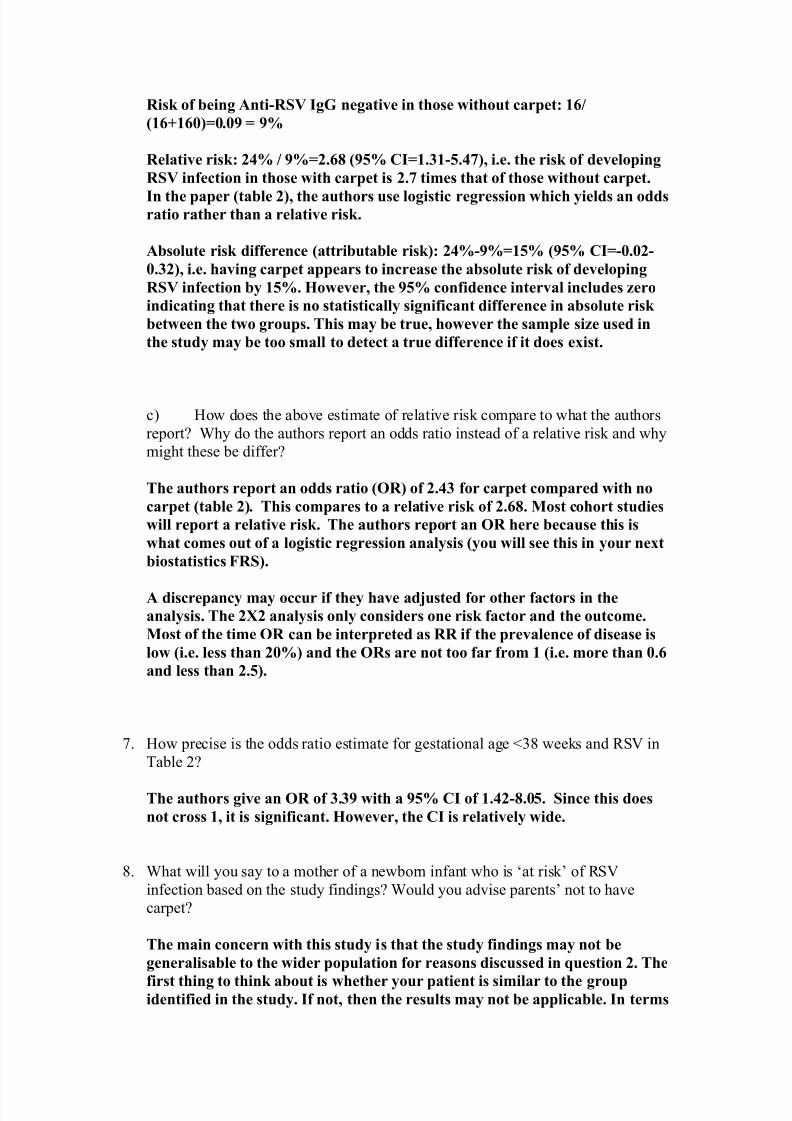
Risk of being Anti-RSV IgG negative in those without carpet: 16/

(16+160)=0.09 = 9%

Relative risk: 24% / 9%=2.68 (95% CI=1.31-5.47), i.e. the risk of developing

RSV infection in those with carpet is 2.7 times that of those without carpet.

In the paper (table 2), the authors use logistic regression which yields an oddsratio rather than a relative risk.

Absolute risk difference (attributable risk): 24%-9%=15% (95% CI=-0.02-

0.32), i.e. having carpet appears to increase the absolute risk of developing

RSV infection by 15%. However, the 95% confidence interval includes zero

indicating that there is no statistically significant difference in absolute risk

between the two groups. This may be true, however the sample size used in

the study may be too small to detect a true difference if it does exist.

c) How does the above estimate of relative risk compare to what the authors

report? Why do the authors report an odds ratio instead of a relative risk and why

might these be differ?

The authors report an odds ratio (OR) of 2.43 for carpet compared with no

carpet (table 2). This compares to a relative risk of 2.68. Most cohort studies

will report a relative risk. The authors report an OR here because this is

what comes out of a logistic regression analysis (you will see this in your next

biostatistics FRS).

A discrepancy may occur if they have adjusted for other factors in the

analysis. The 2X2 analysis only considers one risk factor and the outcome.

Most of the time OR can be interpreted as RR if the prevalence of disease is

low (i.e. less than 20%) and the ORs are not too far from 1 (i.e. more than 0.6

and less than 2.5).

7. How precise is the odds ratio estimate for gestational age <38 weeks and RSV in

Table 2?

The authors give an OR of 3.39 with a 95% CI of 1.42-8.05. Since this does

not cross 1, it is significant. However, the CI is relatively wide.

8. What will you say to a mother of a newborn infant who is ‘at risk’ of RSV

infection based on the study findings? Would you advise parents’ not to have

carpet?

The main concern with this study is that the study findings may not be

generalisable to the wider population for reasons discussed in question 2. The

first thing to think about is whether your patient is similar to the groupidentified in the study. If not, then the results may not be applicable. In terms



of the increased risk of developing RSV infection the OR is relatively large;

however the confidence interval is wide. Whether an infant will benefit from

not having carpet depends on the size and the validity of the attributable risk

estimate. In question 6 we estimated that the attributable risk was 15%. This

means that if we removed carpets in the population then 15% of RSV

infection might be avoided. If we consider the 95% confidence interval thereis no statistically significant difference in absolute risk between the two

groups (95% CI includes zero) and so there may be no benefit to those at risk

from removing exposure to carpets. Even if the result were significant, we

cannot say for sure that an individual infant will benefit because there may

be other factors not included in the research that may be responsible for

infection. All we can say in this case is that removing carpets may be

beneficial.





the full details of the sampling and sample size calculation; this is a common

theme and indicates that you need to have some initiative to do critical

appraisal properly.

3. a) Was there a clearly identified comparison group that was similar

with respect to important determinants of outcome other than the one(s) of

interest?

We are told that the gender distribution between cases and controls is the

same however the mean age of the controls is older than the cases (21.4

year vs. 19.4 years). If age is associated with serious suicide attempt then

the association between the risk factors examined and the suicide attempt

may be due age not the proposed risk factors. The authors recognized age

as a potential confounder and controlled for this by including age in the

logistic regression analysis. They even examined the significantassociations (SES and education) in cases and controls within the 18-24

age group and found similar statistically significant results (although the

p-values were only shown).

b) Could confounding explain the association seen between the risk factors

examined in this study and serious attempted suicide?

As mentioned in Q3(a) age is a potential confounder and this was

controlled for in the analysis. We are also told that occupation, religion,

income, and ethnicity are significant in the bivariate analysis and that

these were no longer significant in the multivariate analysis. Hence, these

factors were associated with serious suicide attempt largely by virtue of

their associations with the participants’ socioeconomic status and

education. The could be residual confounding due to the way that

socioeconomic status and education were defined since there are many

other ways of measuring these. However, confounding is unlikely to

account for the strong association observed in this study.

c) Have the authors attempted to control for any confounding?

As described in Q3(a) and Q3(b) the authors have made an attempt tocontrol for potential confounders. However, other confounders such as

existing mental illness, childhood experiences (e.g. abuse), personality,

medication use, drug use, social support, and other environmental factors

are also potential confounders. Again, confounding is unlikely to account

for the strong association observed in this study.

Students should be aware that if the OR is greater than 3 then

confounding alone is unlikely to account for the association. This means

that the association is likely to be real but the size of the OR may be

different if confounders are taken into account.



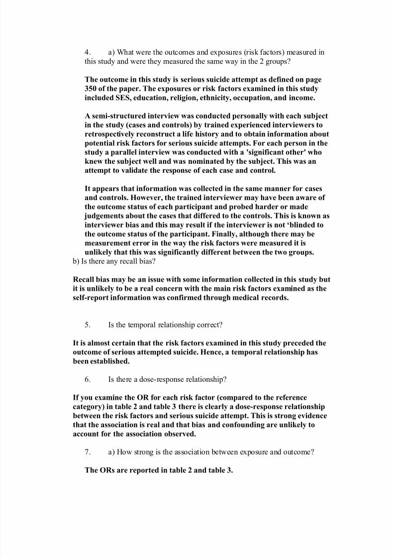
4. a) What were the outcomes and exposures (risk factors) measured in

this study and were they measured the same way in the 2 groups?

The outcome in this study is serious suicide attempt as defined on page

350 of the paper. The exposures or risk factors examined in this study

included SES, education, religion, ethnicity, occupation, and income.

A semi-structured interview was conducted personally with each subject

in the study (cases and controls) by trained experienced interviewers to

retrospectively reconstruct a life history and to obtain information about

potential risk factors for serious suicide attempts. For each person in the

study a parallel interview was conducted with a 'significant other' who

knew the subject well and was nominated by the subject. This was an

attempt to validate the response of each case and control.

It appears that information was collected in the same manner for cases

and controls. However, the trained interviewer may have been aware of the outcome status of each participant and probed harder or made

judgements about the cases that differed to the controls. This is known as

interviewer bias and this may result if the interviewer is not ‘blinded to

the outcome status of the participant. Finally, although there may be

measurement error in the way the risk factors were measured it is

unlikely that this was significantly different between the two groups.

b) Is there any recall bias?

Recall bias may be an issue with some information collected in this study but

it is unlikely to be a real concern with the main risk factors examined as the

self-report information was confirmed through medical records.

5. Is the temporal relationship correct?

It is almost certain that the risk factors examined in this study preceded the

outcome of serious attempted suicide. Hence, a temporal relationship has

been established.

6. Is there a dose-response relationship?

If you examine the OR for each risk factor (compared to the reference

category) in table 2 and table 3 there is clearly a dose-response relationship

between the risk factors and serious suicide attempt. This is strong evidence

that the association is real and that bias and confounding are unlikely to

account for the association observed.

7. a) How strong is the association between exposure and outcome?

The ORs are reported in table 2 and table 3.



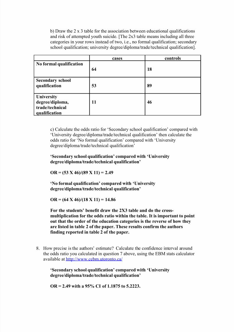
b) Draw the 2 x 3 table for the association between educational qualifications

and risk of attempted youth suicide. [The 2x3 table means including all three

categories in your rows instead of two, i.e., no formal qualification; secondary

school qualification; university degree/diploma/trade/technical qualification].

cases controlsNo formal qualification

64 18

Secondary school

qualification 53 89

University

degree/diploma,

trade/technical

qualification

11 46

c) Calculate the odds ratio for ‘Secondary school qualification’ compared with

‘University degree/diploma/trade/technical qualification’ then calculate the

odds ratio for ‘No formal qualification’ compared with ‘University

degree/diploma/trade/technical qualification’

‘Secondary school qualification’ compared with ‘University


OR = (53 X 46)/(89 X 11) = 2.49

‘No formal qualification’ compared with ‘University


OR = (64 X 46)/(18 X 11) = 14.86

For the students’ benefit draw the 2X3 table and do the cross-

multiplication for the odds ratio within the table. It is important to point

out that the order of the education categories is the reverse of how they

are listed in table 2 of the paper. These results confirm the authors

finding reported in table 2 of the paper.

8. How precise is the authors’ estimate? Calculate the confidence interval around

the odds ratio you calculated in question 7 above, using the EBM stats calculator

available at http://www.cebm.utoronto.ca/

‘Secondary school qualification’ compared with ‘University


OR = 2.49 with a 95% CI of 1.1875 to 5.2223.





‘No formal qualification’ compared with ‘University


OR = 14.86 with a 95% CI of 6.4167 to 34.4536.

As can been seen the confidence intervals are relatively wide but stillsignificant. A larger sample size would provide a more precise estimate of

the true population odds ratio.

9. Do you accept the results of the study?

Overall the internal validity of the study is good; however there is likely to be

residual confounding as discussed above. The generalisability of the study

findings is questionable since we are not given full details of the sampling

methods used for the parent study. The results may only be applicable to a

particular demographic with the NZ population.

Documents

Summary Weeks 1-6