Embed Size (px)
Citation preview
1
JACConjunction Assessment
François LAPORTEOperational Flight Dynamics
CNES Toulouse
SSA Operators’ WorkshopDenver, Colorado
November 3-5, 2016
SSA Operators’ Workshop - November 3-5, 2016 – Denver, Colorado 2
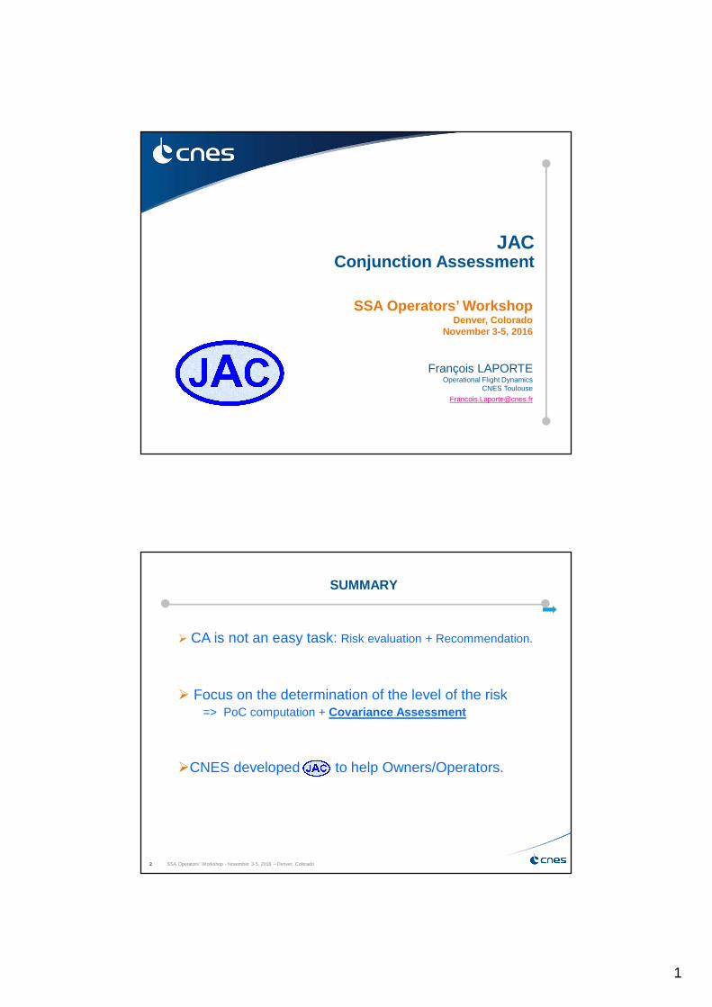
SUMMARY
� CA is not an easy task: Risk evaluation + Recommendation.
� Focus on the determination of the level of the risk => PoC computation + Covariance Assessment
�CNES developed JAC to help Owners/Operators.

2
SSA Operators’ Workshop - November 3-5, 2016 – Denver, Colorado 3
C D M
Space Surveillance Network
JSpOC
Precise and complete catalog
Screening – Information Messages generation
The current situation:Since 2009 JSpOC distributes CM to O/O
SSA Operators’ Workshop - November 3-5, 2016 – Denver, Colorado 4
The current situation:Since 2009 JSpOC distributes CM to O/O
What is a JSpOC’s CDM:� The best available data to avoid collision in space:
� Takes benefit of the US SP catalog;� Is distributed to all O/O;
� A description of a forecasted conjunction :� TCA: Time of Closest Approach;� Orbit information of the 2 objects:
o Position / Velocity at TCA;o Covariance;o Orbit Determination characteristics;
� Information on the size of the object;� Generated with geometric criteria (Miss distance & Radial separation):
� Emergency criteria, up to 3 days before TCA:o LEO: 1 km / 200 m;o GEO: 10 km / 5 km;
� Large criteria (95% capture screening):o LEO: 50 km / 2 km (maximum value), up to 7 days before TCA;o GEO: 360 km / 12 km, up to 14 days before TCA;

3
SSA Operators’ Workshop - November 3-5, 2016 – Denver, Colorado 5
The current situation:Since 2009 JSpOC distributes CM to O/O
But a CDM
� is NOT a conjunction ALERT:� No need to maneuver for each CDM received:
o Emergency criteria: ~30 CM/Year/Satellite;o Large criteria: ~3000 CM/Year/Satellite.
� Need to “evaluate” each CDM to detect a HIE according to O/O criteria;
� is NOT an avoidance maneuver recommendation:� The real need is for an asset, on average:
o LEO: ~1 maneuver per Year;o GEO: ~1 maneuver every 10 Years.
SSA Operators’ Workshop - November 3-5, 2016 – Denver, Colorado 6
I. CDM automatic acquisition and check ;
II. Analysis of incoming CDMs to detect HIE ;
III. Determination of the avoidance action.
Acquisition / Monitoring functionCovariance matrices validityRe-computation of relative geometryCloser approaches detection around TCA
The current situation:Since 2009 JSpOC distributes CM to O/O
An Operational Conjunction Assessment process is:
Dedicated maneuver analysis windows:• to size the avoidance maneuver;• to evaluate the effect on all other future conjunctions.
4
SSA Operators’ Workshop - November 3-5, 2016 – Denver, Colorado 7
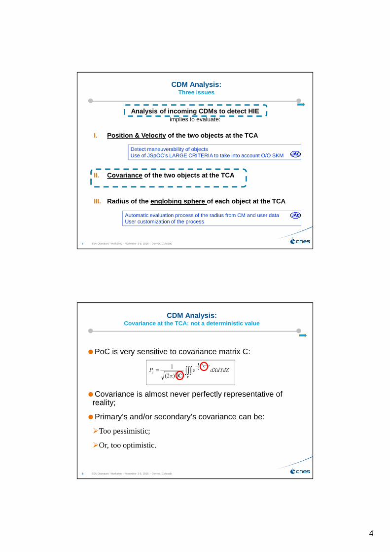
CDM Analysis:Three issues
Analysis of incoming CDMs to detect HIEimplies to evaluate:
I. Position & Velocity of the two objects at the TCA
II. Covariance of the two objects at the TCA
III. Radius of the englobing sphere of each object at th e TCA
Detect maneuverability of objects Use of JSpOC’s LARGE CRITERIA to take into account O/O SKM
Automatic evaluation process of the radius from CM and user dataUser customization of the process
SSA Operators’ Workshop - November 3-5, 2016 – Denver, Colorado 8
�Covariance is almost never perfectly representative of reality;
�Primary’s and/or secondary’s covariance can be:
�Too pessimistic;
�Or, too optimistic.
�PoC is very sensitive to covariance matrix C:
CDM Analysis:Covariance at the TCA: not a deterministic value

5
SSA Operators’ Workshop - November 3-5, 2016 – Denver, Colorado 9
OD 1Pos1Vit1
Cov1
OD 2Pos2
Vit2Cov2
OD 3Pos3
Vit3Cov3
P1
P2t3t2t1
time
3 Orbit Determination Updates (with Cov. Matrix), of the position at T
P3
P1P2P3
P1
P2
P3
Expected evolution in Local Orbital Frame of OD 3
Too pessimistic covariance Too optimistic covariance
CDM Analysis:Covariance at the TCA: not a deterministic value
T
SSA Operators’ Workshop - November 3-5, 2016 – Denver, Colorado 10
CDM Analysis:Covariance at the TCA: PoC* for a PoC analysis
� Definition of the PoC* (expanded PoC):
� PoC(Kp, Ks) gives the PoC as a function of scale coefficients:
» with C = Kp Cp + Ks Cs;
» Kp for the Primary and Ks for the Secondary, are independent scale factors applied to covariance;
� PoC* is the Maximum value of PoC(Kp, Ks) with Kp and Ks in a given interval.
� PoC analysis:
� analysis of the function PoC(Kp, Ks), with Kp and Ks in a given interval;
�determination of the realistic values of Kp and Ks, knowing the OD parameters:
» Number of observations, residuals, weighted root mean squared, energy dissipation rate, …
» Evolution of the OD from updated CDM.

6
SSA Operators’ Workshop - November 3-5, 2016 – Denver, Colorado 11
CDM Analysis:Covariance at the TCA: PoC* for a PoC analysis
Covariance sensitivity analysis on PoC(Kp, Ks)
PoC scale: from 10-0 to 10-10
If Primary’s or Secondary’s covariance is optimistic the risk is under-estimated If Primary’s and
Secondary’s covariance are pessimistic the risk is over-estimated
Example of display: Kp in [0.5 ; 3.] and Ks in [0.5 ; 3.]
Kp
Ks
(1 , 1)
3.0
3.00.5
0.2
SSA Operators’ Workshop - November 3-5, 2016 – Denver, Colorado 12
CDM Analysis:Covariance at the TCA: PoC analysis - Real example
Time tagged received CDMs:GNOSE = O/O for Primary; JSpOC for secondary
Notice = # hours before TCA
PoC always < CRITERIA = 5. 10-4
Decision to perform an avoidance maneuver because … it is a risky conjunction.
This is the default values considered at CNES
CM Analysis Main Window
Example of a dangerous conjunction identified thank s to the expanded PoC analysis.
A click here, opens the dedicated PoC analysis window.

7
SSA Operators’ Workshop - November 3-5, 2016 – Denver, Colorado 13
PoC scale: from 10-0 to 10-10
� As soon as Kp & Ks <1, PoC > CRITERIA;
� If Kp and Ks < 0.6 then PoC > 10-3
The analyst must answer :Kp < 0,9 and Ks < 0,8 : realistic ?
Let’s have a look at the evolution of Primary’s and Secondary’s covariance …
PoC Analysis Window White when cell’s PoC > 5. 10-4
Kp=0.9 Ks=0.8 => PoC = 5.4 10-4
Kp
Ks
(1 , 1)
Standard PoC = 3.7 10-4
Kp=0.7 Ks=0.5 => PoC = 1. 10-3
4.0
4.00.2
0.2
CDM Analysis:Covariance at the TCA: PoC analysis - Real example
SSA Operators’ Workshop - November 3-5, 2016 – Denver, Colorado 14
Primary dispersions evolution visualization
CDM Analysis:Covariance at the TCA: PoC analysis - Real example
Secondary dispersions evolution visualization
The covariance of both objects are pessimistic: the PoC can realistically be greater than the CRITERIA.
⇒ This is a risky conjunction⇒ A classical analysis would have miss this risk
Kp
Ks

8
SSA Operators’ Workshop - November 3-5, 2016 – Denver, Colorado 15
CDM Analysis:Covariance at the TCA: PoC forecast - Real example
The high risk have been anticipated thanks to the P oC analysis window
CDM #6: PoC still below blue PoC* is orange.
When the orange area if bottom/left, the risk usually increases when the geometry is steady:� Because dispersions reduce.
Very useful to anticipate operational activities.
SSA Operators’ Workshop - November 3-5, 2016 – Denver, Colorado 16
-III- CDM Analysis:Covariance Determination
Covariance determination
� It can be an output of the Orbit Determination process:
o It must include in the Orbit Determination process
o very often it is an under-estimation of the reality.
� Post analysis of the O/O ephemeris: from historical set of ephemerides
A
B
C
D
E
F
1 day extrapolation: A, B, C
2 days extrapolation: D, E
3 days extrapolation: F
Day 1
Day 2
Day 4
Day 3
⇒ provides statistics of dispersion in the RIN local orbital frame;
⇒ from this statistics we can create a “variance abacus”.
Determinated orbit Extrapolated orbit
Day 1 Day 4Day 3Day 2

9
SSA Operators’ Workshop - November 3-5, 2016 – Denver, Colorado 17
-III- CDM Analysis:Covariance Determination
Variance abacus: basic function
gives the evolution of variance (in meters) in the threedirections (Radial, In-track and Normal) of orbital localframe as a function of extrapolation duration (in days).
For a given extrapolation duration, such function (the green orthe red one in the above example) gives the evolution ofvariance (in meters) in the three directions (Radial, In-trackand Normal) of orbital local frame as a function of On orbitPosition (in degree).
⇒Takes into account the evolution of dispersions along theorbit due to the non-uniformity of distribution of sensorsproviding the measurements for the OD.
⇒This lead to a more realistic computation and reduc e the uncertainties on some orbit positions.
Variance abacus: as a function of On Orbit Position
SSA Operators’ Workshop - November 3-5, 2016 – Denver, Colorado 18
Conclusion
Evolution of CA Process:� In the past: Miss distance & relative geometry
� Its minimum does not always represent the highest risk;� Doesn’t take into account Position uncertainties:
⇒ Not a valid criteria⇒ Need to take into account position uncertainties (i.e. covariance)
� Now: PoC � Takes into account Positions uncertainties: very good improvement;� But relies on the realism of the covariance …
⇒ Can hide dangerous situations / Can lead to undersize avoidance action ⇒ Need to take into account covariance uncertainties
� Next step: PoC + Covariance Assessment� Takes into account covariance uncertainties

10
SSA Operators’ Workshop - November 3-5, 2016 – Denver, Colorado 19
Conclusion
� CA a fully automatic process … not yet: � Can miss some risks / undersize avoidance action;� Can lead to too many avoidance events:
⇒ The final analysis must be a manual analysis.
� JAC can help O/O to perform this manual analysis
� JAC is distributed by CNES in 2 levels: � Basic (“to be aware of the situation”) for free;� Expert (“to take and validate a decision”) for an annual fee.