Summary about Convolution Lecture 4: Smoothingrtc12/CSE486/lecture04_6pp.pdf · Summary about Convolution ... –Sensor noise ... Robert Collins Modeling Image Noise Simple model:

1

CSE486, Penn StateRobert Collins

Lecture 4:Smoothing

Related text is T&V Section 2.3.3 and Chapter 3


Summary about Convolution

Computing a linear operator in neighborhoods centered at eachpixel. Can be thought of as sliding a kernel of fixed coefficientsover the image, and doing a weighted sum in the area of overlap.

things to take note of: full : compute a value for any overlap between kernel and image (resulting image is bigger than the original) same: compute values only when center pixel of kernel aligns with a pixel in the image (resulting image is same size as original)

convolution : kernel gets rotated 180 degrees before sliding over the image cross-correlation: kernel does not get rotated first

border handling methods : defining values for pixels off the image


Problem: Derivatives and Noise

M.Hebert, CMU


Problem: Derivatives and Noise

M.Nicolescu, UNR

Increasing noise

•First derivative operator is affected by noise

• Numerical derivatives can amplify noise! (particularly higher order derivatives)


Image Noise

• Fact: Images are noisy

• Noise is anything in the image that we arenot interested in

• Examples:– Light fluctuations

– Sensor noise

– Quantization effects

– Finite precision

O.Camps, PSU


Modeling Image Noise

Simple model: additive RANDOM noise

I(x,y) = s(x,y) + ni

Where s(x,y) is the deterministic signal ni is a random variable

Common Assumptions: n is i.i.d for all pixels n is zero-mean Gaussian (normal) E(n) = 0 var(n) = σ2

E(ni nj) = 0 (independence)

O.Camps, PSU

Note: This really only models the sensor noise.

2


Forsyth and Ponce

Example: Additive Gaussian Noisemean 0, sigma = 16


Empirical Evidence

Mean = 164 Std = 1.8


Other Noise Models

•Multiplicative noise: ),(),(ˆ),( jiNjiIjiI ⋅=

•Impulse (“shot”) noise (aka salt and pepper):

≥−+

<=

lxiiyi

lxjiIjiI

)(

if),(ˆ),(

minmaxmin

O.Camps, PSU

See Textbook

We won’t cover them. Just be aware they exist!!


Smoothing Reduces Noise

The premise of data smoothing is that one is measuringa variable that is both slowly varying and also corruptedby random noise. Then it can sometimes be useful toreplace each data point by some kind of local average ofsurrounding data points. Since nearby points measurevery nearly the same underlying value, averaging canreduce the level of noise without (much) biasing thevalue obtained.

From Numerical Recipes in C:


Today: Smoothing Reduces Noise

Image patch Noisy surface

smoothing reduces noise,giving us (perhaps) a more accurate intensity surface.


Preview

• We will talk about two smoothing filters– Box filter (simple averaging)

– Gaussian filter (center pixels weighted more)

3


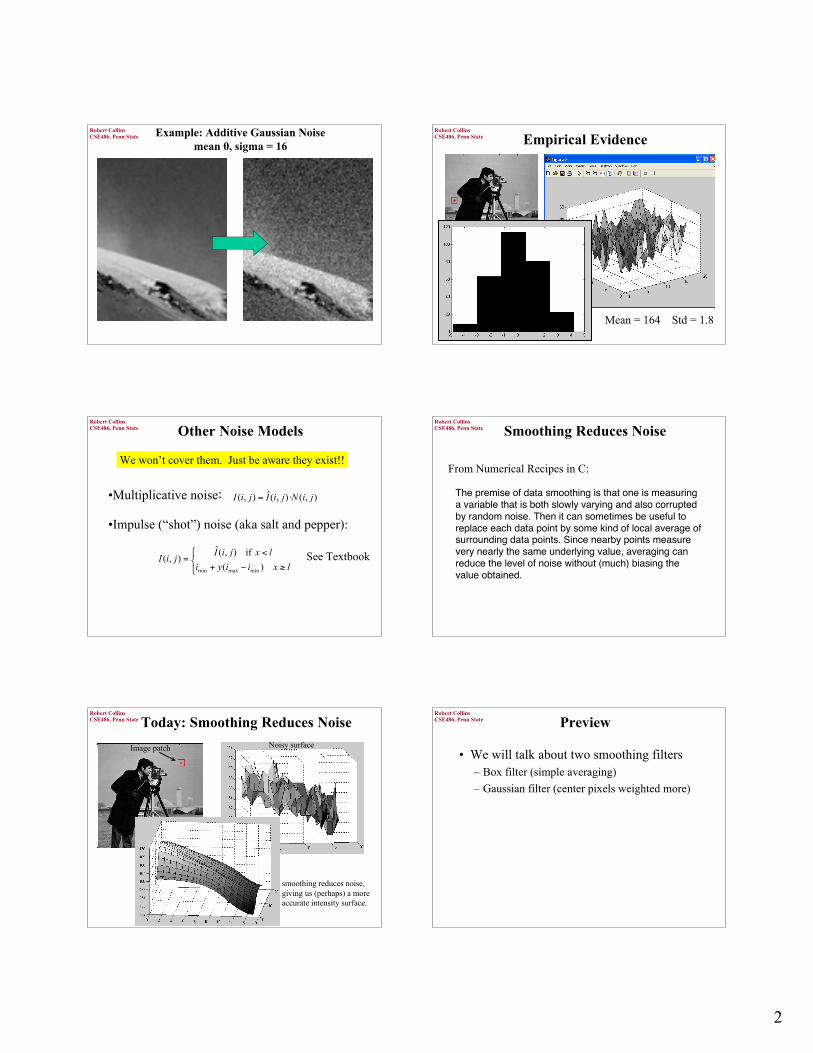
Averaging / Box Filter

• Mask with positiveentries that sum to 1.

• Replaces each pixelwith an average of itsneighborhood.

• Since all weights areequal, it is called aBOX filter.

1111 11

Box filterBox filter

1/91/9

1111 11

1111 11

O.Camps, PSU

since this is a linear operator, we can take the average around each pixel by convolving the image with this 3x3 filter!

important point:


Why Averaging Reduces Noise

O.Camps, PSU

• Intuitive explanation: variance of noise in the average is smaller than variance of the pixel noise (assuming zero-mean Gaussian noise).

• Sketch of more rigorous explanation:


Smoothing with Box Filter

original Convolved with 11x11 box filter

Drawback: smoothing reduces fine image detail


Important Point about Smoothing

Averaging attenuates noise (reduces the variance), leading to a more “accurate” estimate.

However, the more accurate estimate is of the mean ofa local pixel neighborhood! This might not be what you want.

Balancing act: smooth enough to “clean up” the noise,but not so much as to remove important image gradients.


Gaussian Smoothing Filter

• a case of weighted averaging– The coefficients are a 2D Gaussian.

– Gives more weight at the central pixels and lessweights to the neighbors.

– The farther away the neighbors, the smaller theweight.

O.Camps, PSU

Confusion alert: there are now two Gaussians being discussed here (one for noise, one for smoothing). They are different.



An isotropic (circularly symmetric) Gaussian:

4


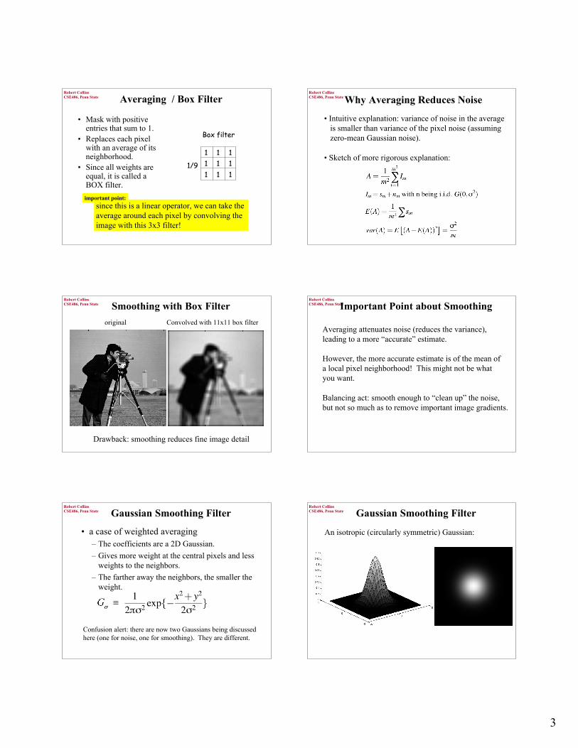
In Matlab>> sigma = 1

sigma =

1

>> halfwid = 3*sigma

halfwid =

3

>> [xx,yy] = meshgrid(-halfwid:halfwid, -halfwid:halfwid);>> tmp = exp(-1/(2*sigma^2) * (xx.^2 + yy.^2))

tmp =

0.0001 0.0015 0.0067 0.0111 0.0067 0.0015 0.0001 0.0015 0.0183 0.0821 0.1353 0.0821 0.0183 0.0015 0.0067 0.0821 0.3679 0.6065 0.3679 0.0821 0.0067 0.0111 0.1353 0.6065 1.0000 0.6065 0.1353 0.0111 0.0067 0.0821 0.3679 0.6065 0.3679 0.0821 0.0067 0.0015 0.0183 0.0821 0.1353 0.0821 0.0183 0.0015 0.0001 0.0015 0.0067 0.0111 0.0067 0.0015 0.0001

Note: we have not included the normalization constant. Values of a Gaussian should sum to one. However, it’sOK to ignore the constant since you can divide by it later.



Just another linear filter. Performs a weighted average.Can be convolved with an image to produce a smoother image.

>> sigma = 1

sigma =

1

>> halfwid = 3*sigma

halfwid =

3>> [xx,yy] = meshgrid(-halfwid:halfwid, -halfwid:halfwid);>> gau = exp(-1/(2*sigma^2) * (xx.^2 + yy.^2))

gau =

0.0001 0.0015 0.0067 0.0111 0.0067 0.0015 0.0001 0.0015 0.0183 0.0821 0.1353 0.0821 0.0183 0.0015 0.0067 0.0821 0.3679 0.6065 0.3679 0.0821 0.0067 0.0111 0.1353 0.6065 1.0000 0.6065 0.1353 0.0111 0.0067 0.0821 0.3679 0.6065 0.3679 0.0821 0.0067 0.0015 0.0183 0.0821 0.1353 0.0821 0.0183 0.0015 0.0001 0.0015 0.0067 0.0111 0.0067 0.0015 0.0001


Gaussian Smoothing Example

original sigma = 3


Box vs Gaussian

box filter gaussian


Box vs Gaussian

box filter gaussian

Note: Gaussian is a true low-pass filter, so won’t causehigh frequency artifacts. See T&V Chap3 for more info.

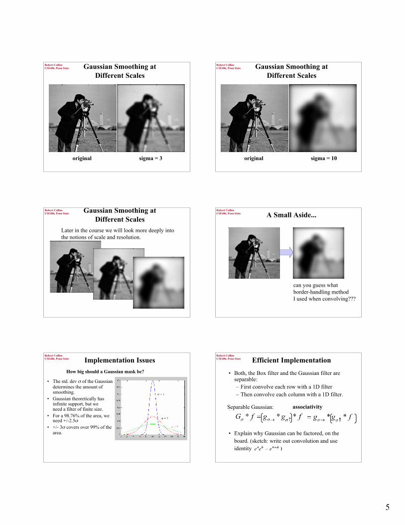
CSE486, Penn StateRobert Collins Gaussian Smoothing at

Different Scales

original sigma = 1

5


original sigma = 3

Gaussian Smoothing atDifferent Scales


Different Scales

original sigma = 10


Different Scales

Later in the course we will look more deeply intothe notions of scale and resolution.


A Small Aside...

can you guess what border-handling method I used when convolving???


Implementation Issues

• The std. dev σ of the Gaussiandetermines the amount ofsmoothing.

• Gaussian theoretically hasinfinite support, but weneed a filter of finite size.

• For a 98.76% of the area, weneed +/-2.5σ

• +/- 3σ covers over 99% of thearea.

O.Camps, PSU

How big should a Gaussian mask be?


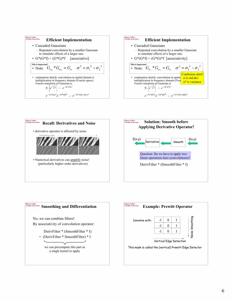
Efficient Implementation

• Both, the Box filter and the Gaussian filter areseparable:– First convolve each row with a 1D filter– Then convolve each column with a 1D filter.

• Explain why Gaussian can be factored, on theboard. (sketch: write out convolution and useidentity )

Separable Gaussian: associativity

6


Efficient Implementation• Cascaded Gaussians

– Repeated convolution by a smaller Gaussianto simulate effects of a larger one.

• G*(G*f) = (G*G)*f [associative]

• Note:

• explanation sketch: convolution in spatial domain ismultiplication in frequency domain (Fourier space).Fourier transform of Gaussian is

This is important!


Efficient Implementation• Cascaded Gaussians

– Repeated convolution by a smaller Gaussianto simulate effects of a larger one.

• G*(G*f) = (G*G)*f [associativity]

• Note:

• explanation sketch: convolution in spatial domain ismultiplication in frequency domain (Fourier space).Fourier transform of Gaussian is

This is important!

Confusion alert! σ is std.dev σ2 is variance


Recall: Derivatives and Noise

M.Nicolescu, UNR

Increasing noise

• derivative operator is affected by noise

• Numerical derivatives can amplify noise! (particularly higher order derivatives)

CSE486, Penn StateRobert Collins Solution: Smooth before

Applying Derivative Operator!

SmoothSmoothDerivativeDerivativeI(x,y)I(x,y)E(x,y)E(x,y)

O.Camps, PSU

Question: Do we have to apply twolinear operations here (convolutions)?

DerivFilter * (SmoothFilter * I)


Smoothing and Differentiation

DerivFilter * (SmoothFilter * I)

= (DerivFilter * SmoothFilter) * I

No, we can combine filters!

By associativity of convolution operator:

we can precompute this part asa single kernel to apply


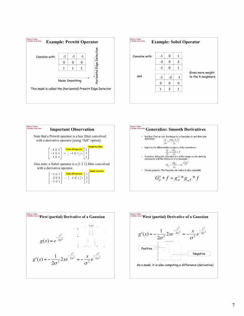
Example: Prewitt Operator

Convolve with:Convolve with: -1-1 00 11

-1-1 00 11

-1-1 00 11

Vertical Edge DetectionVertical Edge Detection

Noi

se S

moo

thin

gN

oise

Sm

ooth

ing

This mask is called the (vertical) Prewitt Edge DetectorThis mask is called the (vertical) Prewitt Edge Detector

O.Camps, PSU

7


Example: Prewitt Operator

Convolve with:Convolve with: -1-1 -1-1 -1-1

00 00 00

11 11 11

Noise SmoothingNoise Smoothing

Hor

izon

tal E

dge

Det

ecti

onH

oriz

onta

l Edg

e D

etec

tion

This mask is called the (horizontal) Prewitt Edge DetectorThis mask is called the (horizontal) Prewitt Edge Detector

O.Camps, PSU


Example: Sobel Operator

Convolve with:Convolve with: -1-1 00 11

-2-2 00 22

-1-1 00 11

andand -1-1 -2-2 -1-1

00 00 00

11 22 11

Gives more weightGives more weightto the 4-neighborsto the 4-neighbors

O.Camps, PSU


Important Observation

Note that a Prewitt operator is a box filter convolved with a derivative operator [using “full” option].

Also note: a Sobel operator is a [1 2 1] filter convolved with a derivative operator.

Simple box filter

Simple Gaussian

Finite diff operator

Finite diff operator


Generalize: Smooth Derivatives

M.Hebert, CMU


First (partial) Derivative of a Gaussian

2

2

2)( σ

x

exg−

=

2

2

2

2

22

222

2

1)(' σσ

σσ

xx

ex

xexg−−

−=−=

O.Camps, PSU


First (partial) Derivative of a Gaussian

2

2

2

2

22

222

2

1)(' σσ

σσ

xx

ex

xexg−−

−=−=

PositivePositive

NegativeNegative

As a mask, it is also computing a difference (derivative)As a mask, it is also computing a difference (derivative)

O.Camps, PSU

8


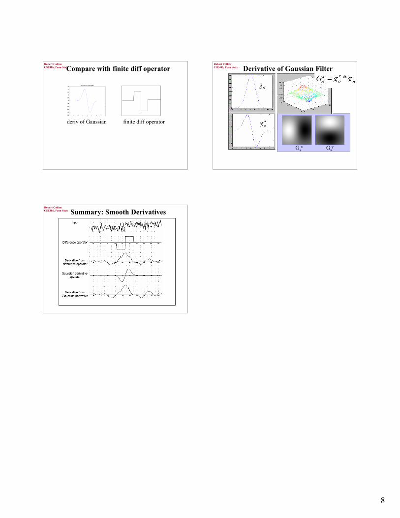
Compare with finite diff operator

deriv of Gaussian finite diff operator


Derivative of Gaussian Filter

M.Hebert, CMU

Gsx Gs

y


Summary: Smooth Derivatives

M.Hebert, CMU

Documents

Summary about Convolution Lecture 4: Smoothingrtc12/CSE486/lecture04_6pp.pdf · Summary about Convolution ... –Sensor noise ... Robert Collins Modeling Image Noise Simple model: