SUBSURFACE GEOLOGY OF ARSENIC-BEARING

PERMIAN SEDIMENTARY ROCKS IN

THE GARBER-WELLINGTON INTERVAL OF THE

CENTRAL OKLAHOMA AQUIFER,

CLEVELAND COUNTY,

OKLAHOMA

By

BEN NICHOLAS ABBOTT

Bachelor of Science

Oklahoma State University

Stillwater, Oklahoma

2002

Submitted to the Faculty of the Graduate College of Oklahoma State University in partial fulfillment

of the requirements for the degree of MASTER OF SCIENCE

December, 2005

ii

SUBSURFACE GEOLOGY OF ARSENIC-BEARING

PERMIAN SEDIMENTARY ROCKS IN

THE GARBER-WELLINGTON INTERVAL OF THE

CENTRAL OKLAHOMA AQUIFER,

CLEVELAND COUNTY,

OKLAHOMA

Thesis Approved:

Stanley T. Paxton

Thesis Advisor

James Puckette

Surinder Sahai

Gordon Emslie Dean of the Graduate College

iii

COPYRIGHT

By

Ben Nicholas Abbott

December, 2005

iv

ACKNOWLEDGEMENTS

I wish to express my sincerest gratitude to my advisor, Dr. Stan Paxton, whose

help was invaluable and instrumental to the completion of this thesis. I also would like to

thank my committee, Dr. Jim Puckette and Dr. Surinder Sahai for their assistance. Jim

Roberts’ help and expertise were priceless. And this thesis would certainly not have been

possible without support from the EPA. Finally, thanks to my lovely wife, Erin Abbott,

for putting up with me during the course of this work.

v

TABLE OF CONTENTS

Chapter Page I. INTRODUCTION………………………………….……………………..…………1 II. PURPOSE AND OBJECTIVES…………………….……………..………………..6 III. BACKGROUND AND PREVIOUS WORK………………………….….………...8 General Geology…………………………………………………………………8 Hydrogeology…………………………………………………………………...16 IV. METHODOLOGY……….……………………………………….………………..28 Data Acquisition and Interpretation…….………………….…….………....…...28 Construction of Maps and Cross Sections………………….….….……………..35 V. RESULTS AND DISCUSSION……………………………….….………………...38

Well Log Data Summary………………………………………………………...38 Maps…………………………………………………………………..……........39

Large Scale Cross Sections.……….……………………………………….…….50 Small Scale Cross Sections and Well Log Response Patterns…………………..50

VI. CONCLUSIONS AND SUGGESTIONS FOR FUTURE WORK…………….…..59 REFERENCES CITED………………………………………………………………….62 APPENDICES…………………………………………………………………………...64

APPENDIX A – WELL HEADER DATA……………………………………...65 APPENDIX B – FORMATION TOP DATA ………………………….……….74 APPENDIX C – NORMAN WATER WELL DATA…………………………..85 APPENDIX D – UNIVERSITY OF OKLAHOMA WATER WELL DATA….93 APPENDIX E – GARBER-WELLINGTON CONTACT STUDY……………102

vi

LIST OF TABLES

Table Page 1. Summary Statistics for OU and Norman Wells……………………………………….46

vii

LIST OF FIGURES

Figure Page 1. Location Map, Central Oklahoma Aquifer……………………………………...…….2 2. Stratigraphic Column, Central Oklahoma Aquifer………………………....…...…….5 3. Garber Sandstone Map and Cross Section (1928)...………………………….....…...21 4. Oklahoma City Anticline and Associated Structures (1968)….…...………………...22 5. Positions of Gamma Ray Cutoff Lines……………………………………....………31 6. Type Log, Garber-Wellington Aquifer……………………………………..…..........34 7. Type Log, Garber Sandstone……………………………………………..………….34 8. Comparison of OU and Norman Water Wells……………………………………….46 9. Histograms, Units A, B, and C, Net Clean Sandstone Content……………..….……47 10. Histograms, Units A, B, and C, Percent Clean Sandstone Content……………….…48 11. Histograms, Units A, B, and C, Percent Shaly Sandstone Content…………...…..…49 12. Location of Large Scale Cross Sections……………………………………………..51 13. Location of Small Scale Cross Sections……………………………………………..52 14. Detail of Cross Section H-H’………………………………………………………...54 15. Detail of Cross Section D-D’………………………………………………………...54 16. Potential Arsenic Zones Map…………………………………………………….…..61

viii

LIST OF PLATES

Plate 1. Base Map..……………………………………………………………………..In Pocket 2. Structure Map, Top of Garber Sandstone and Garber Isopach…………….….In Pocket 3A. Garber Lithofacies Maps……….......…………………………….…….……In Pocket 3B. Percent Shaly Sandstone Map with Arsenic Overlay………….………….…In Pocket 4. Residual Trend Structure Maps…......................................................................In Pocket 5. Unit A: Isopach Map, Net Clean Sandstone Map, Percent Clean Sandstone Map,

Percent Shaly Sandstone Map………………...………………………….In Pocket 6. Unit B: Isopach Map, Net Clean Sandstone Map, Percent Clean Sandstone Map,

Percent Shaly Sandstone Map…...……………………………………….In Pocket 7. Unit C: Isopach Map, Net Clean Sandstone Map, Percent Clean Sandstone Map,

Percent Shaly Sandstone Map……………...…………………………….In Pocket 8. Cross Section Line Map..……………………………………………………...In Pocket 9. Cross Sections X-X’ and Y-Y’………………………………………………...In Pocket 10. Cross Sections A-A’ and B-B’…………….………………………...……….In Pocket 11. Cross Sections C-C’ and D-D’…………..…………………………………...In Pocket 12. Cross Sections E-E’ and F-F’………………………………………………...In Pocket 13. Cross Sections G-G’ and H-H’………..……………………………………...In Pocket

1

I.

INTRODUCTION

As an important source of drinking water in central Oklahoma, the Central

Oklahoma Aquifer (COA) has been the focus of much attention in recent years because

of elevated levels of naturally occurring arsenic. The City of Norman, located in

Cleveland County, Oklahoma (Figure 1), obtains its groundwater from the Garber-

Wellington portion of the Central Oklahoma Aquifer; Norman has the second highest

levels of naturally occurring arsenic in drinking water in the United States, exceeded only

by Albuquerque, NM. In 2006, the Environmental Protection Agency (EPA) will lower

the maximum allowable limit of arsenic in drinking water from the current level of 50

ppb to 10 ppb; numerous wells currently producing from the Central Oklahoma Aquifer

will not meet the new standard. The City of Norman would like to remediate the arsenic-

in-drinking-water-problem so that city wells will not have to be taken off line. The city is

also trying to avoid the expense of surface treatment techniques. OSU, in conjunction

with the EPA and the United States Geological Survey (USGS), is evaluating remediation

techniques and preparing preventative guidelines to the City of Norman and other

municipalities that obtain their drinking water from the Central Oklahoma Aquifer.

Previous work by the USGS has indicated that arsenic concentration may be proportional

to the volume of shale in a wellbore (Schlottmann et al., 1998). Therefore, some

approaches to achieving the goal of lowered arsenic levels are: 1) selective production

Central Oklahoma Aquifer

Norman

Figure 1. Location map of the Central Oklahoma Aquifer and surrounding geologic features (modified after George N. Breit, The Diagenetic History of Permian Rocks in the Central Oklahoma Aquifer, in USGS Water-Supply Paper 2357-A)

2

3

of water from low arsenic stratigraphic intervals; 2) squeezing off high-arsenic intervals

in existing wells; and 3) drilling new wells in areas with low arsenic potential. In order to

implement these approaches, the need arises for subsurface mapping of the Garber-

Wellington Aquifer, in terms of lithofacies (sandstone, shale, shaly sandstone) and

sediment packages. This work should provide a better understanding of the Garber

Sandstone and Wellington Formation not only with respect to arsenic, but also with

respect to the depositional system from which the rocks originated. To fulfill the need for

better definition of the geology of the Garber-Wellington Aquifer, this study, along with

two other OSU graduate theses, begins to establish a geologic-stratigraphic framework

for this part of the COA.

With the exception of Quaternary fluvial terrace deposits, all rocks in the Central

Oklahoma Aquifer are Permian (Artinskian, formerly Leonardian) aged. The Garber

Sandstone and the Wellington Formation are the most significant water-bearing units in

the Central Oklahoma Aquifer; other formations in the COA are the underlying Council

Grove, Chase, and Admire Groups. The aquifer is overlain and in some places confined

by the Hennessey Shale and underlain by the Pennsylvanian Vanoss Formation (Figure

2). The Garber Sandstone and the underlying Wellington Formation consist of

amalgamated lenticular fluvial sandstones interbedded with mudstones, siltstones, and

some conglomerates (Breit et al., 1990). Previous work by the U.S. Geological Survey

has shown that arsenic content in the Garber-Wellington Aquifer is a function of grain-

size, i.e., arsenic concentration is higher where the rocks are finer-grained (Schlottmann

et al., 1998). It has also been suggested by the USGS that arsenic is elevated in

sandstones isolated by finer-grained rocks, due to a lack of flushing-out of these rocks.

4

In this study, the Garber-Wellington Aquifer was analyzed in terms of the geometry,

continuity, and spatial distribution of different lithofacies. The two other OSU theses

focus on the physical properties of the rocks, especially outcrop gamma-ray

measurements, grain size analyses, and whole-rock geochemistry (Gregory Gromadzki),

and outcrop description and mapping (Kathy Kenney). These three studies are intended

to complement each other and enhance understanding of arsenic distribution in the

Garber-Wellington Aquifer through integration of both surface and subsurface work.

Figure 2. Stratigraphic column of the Central Oklahoma Aquifer (modified after George N. Breit, The Diagenetic History of Permian Rocks in the Central Oklahoma Aquifer, in USGS Water-Supply Paper 2357-A)

Cen

tral O

klah

oma

Aqu

ifer

Hennessey Shale

Garber Sandstone and Wellington Formation

Council Grove, Chase, and Admire Groups

Vanoss FormationPENNSYLVANIAN

PER

MIA

N

5

6

II.

PURPOSE AND OBJECTIVES

The primary goal of this study is to provide a geologic and stratigraphic

framework to be used by the USGS and EPA to help remediate the arsenic problem in the

Norman, OK area. These agencies will be able to use the results of this study and its two

counterpart studies as a guideline for selection of new drilling locations, as a means of

possibly locating and isolating arsenic-rich zones, and as input into fluid flow modeling

to be conducted by the USGS. For this study to be helpful in this manner, the Garber-

Wellington aquifer was mapped in terms of structure, thickness, and lithofacies.

Subsurface well logs were the primary source of data, although a minor amount of core

data was also used. From the well logs, cross-sections and maps were constructed to

provide a picture of the subsurface character of the Garber-Wellington Aquifer,

especially with respect to unit continuity and gradations from one lithofacies into another.

The Garber Wellington aquifer is composed of three primary lithofacies as

represented by wireline logs: sandstone, shale, and shaly sandstone. There are also minor

amounts of conglomerates, but these are not mapped in this study because of the

difficulty associated with identifying them using well logs (they are usually too thin). If

arsenic occurrence is associated with finer-grained lithofacies (shaly sandstone and

shale), then mapping the distribution of these lithofacies should provide valuable insight

7

into the relationship between arsenic occurrence and rock type in the Garber-Wellington

Aquifer. Briefly, the objectives of this thesis are to:

1) Construct cross sections through the Garber Sandstone and to use the cross

sections to determine if the rocks of the Garber Sandstone can be correlated (the

units do not contain regional stratigraphic markers),

2) Identify, from the cross sections, continuous sediment packages or units,

3) Map the subsurface structural relief of the upper and lower surfaces of the

Garber Sandstone and any identifiable units within it,

4) Determine and map the amounts of clean sandstone, shaly sandstone, and shale

in the Garber Sandstone (and in its mappable components), in terms of net

thickness, percent lithology, and/or ratios of various lithofacies,

5) Identify areas of prospective low and high arsenic concentration based on the

above maps,

6) Estimate the location and orientation of the main depo-center responsible for the

Garber sediments in the Norman area, and to attempt to track changes in the

system through time (migration of the channel fairway) based on the maps, and

7) Recommend possible remediation strategies based on our understanding of the

geology and stratigraphic framework.

8

III.

BACKGROUND AND PREVIOUS WORK

The Garber-Wellington Aquifer makes up most of the thickness of the Central

Oklahoma Aquifer (COA) and contains most of the aquifer’s fresh water. The COA also

is overlain by the Hennessey Shale and Quaternary alluvium, and underlain by the Chase,

Council Grove, and Admire Groups. In Cleveland County, the Garber-Wellington

Aquifer is confined by the Hennessey Shale to the west, and is unconfined to the east.

The USGS has done much work on the COA; among the conclusions reached from their

investigations is that arsenic is mobilized under high pH conditions, and that high pH

conditions in the COA occur at depth, below the city of Norman. The USGS has also

concluded that the arsenic is contained in the Permian siltstones and mudstones of the

aquifer. Most of this work has focused more on the geochemical aspect of the problem

rather than on the sedimentary framework that makes up the aquifer. The USGS work

will be discussed later in more detail.

General Geology

The study area is located to the south of the Oklahoma City Anticline, a structure

whose development is associated with the Nemaha Ridge and the Anadarko Basin. The

units of the Garber-Wellington dip to the west and are relatively flat lying. However,

several known fault zones surround the study area at depth. The Oklahoma

9

City Anticline is an elongate, anticlinal feature trending north 30 degrees west in southern

Oklahoma County, and is bounded to the east by the Nemaha Fault Zone (Foley, 1934).

In order to show the evolution of our understanding and conception of the Garber

Sandstone and Wellington Formation, the literature will be discussed chronologically.

The earliest papers, from the 1930’s, were written with respect to Permian red beds as

possible oil and gas reservoirs. The earliest work to treat the Garber and Wellington as

an aquifer came in the 1960’s. Most of the modern research (post-1950’s) focuses on the

geochemistry and hydrologic properties of the aquifer.

Some of the earliest work on the Permian in Oklahoma is found in The

Subdivision of the Enid Formation by Aurin, et al. (1926). The Enid Formation was a

term used to describe a sequence of rocks that included much of the Permian section. As

the result of a field conference attended by the Aurin, Officer, Gould, and several other

geologists, the Enid Formation was subdivided into six distinct formations. These

formations, from oldest to youngest, were the Stillwater, Wellington, Garber, Hennessey,

Duncan, and Chickasha. Aurin et al. (1926) give a detailed account of the conclusions

reached at the field conference, and describe each of the formations in detail.

At the time the Aurin et al. (1926) paper was written, the name “Garber

Sandstone” was primarily a local term, and the authors proposed that the name be

formally adopted as a formation name, to describe “a series of red clay shales, red sandy

shales, and red sandstones lying above the Wellington” (p. 794). The authors also state

that the Garber is about 600 feet thick. Also proposed is the usage of Lucien Shale

Member and Hayward Sandstone Member to describe the lower and upper intervals of

the Garber. However, these units do not persist from the area of description (Garfield,

10

western Noble, and western Logan counties) into Cleveland County. The lower Garber,

or Lucien Shale Member, is described as being mostly red shales with a few sandstone

units. In the Norman area, however, the current author found that the lower Garber

contains as much sandstone as the upper Garber.

The Wellington Formation is described by Aurin, et al., in its type locality

(Wellington, KS), as consisting of “drab or gray shale with numerous thin beds of gray

‘mud-stone,’ scattered impure limestones, and clay conglomerates”. Aurin, et al. also

recognize the southward gradation of the Wellington into red beds, stating that as one

moves south, the shales become red, followed by the appearance of sandstones. South of

the Cimarron River, the Wellington has completely changed from its character at the type

locality, consisting there of interbedded red siliciclastic mudstone and sandstone. The top

of the Wellington is given as “the base of the lowest heavy sandstone of the Garber

formation,” and the base of the Wellington is the top of the Herington Limestone. The

thickness of the Wellington is about 600 feet in the northern part of the state.

The name “Stillwater Formation” is used by Aurin, et al. as a collective term,

encompassing what are now referred to as the Council Grove, Chase, and Admire

Groups. The top of the Stillwater Formation is the Herington Limestone and its base is

the Cottonwood Limestone. The authors report a facies change from limestone/shale

dominated to sandstone/shale dominated, as well as a general thickening, as one moves

south from Kansas. Some of the major formation names and divisions described by

Aurin, et al. (1926) are still in use, except for “Stillwater Formation.” Their Garber and

Wellington subunit names are also uncommon.

11

Another of the early papers dealing with Permian rocks in Oklahoma was Lower

Permian Correlations in Cleveland, McClain, and Garvin Counties, Oklahoma, by

Robert H. Dott (1932). Dott’s work was focused mainly on continuing and developing

the work of Aurin, et al. (1926), and he proposed several changes to their subdivision of

the Enid Group. His correlations were based on “lithologic similarity, the sequence of

beds, similar thicknesses” (p. 119). Interestingly, he also mentions the use of zones of

barite roses as regional markers, but this is later refuted by Lloyd Gatewood (1968), who

reported that they do not occur in discrete zones. Dott reports 600 feet of Hennessey

Shale, 200 feet of Garber Sandstone, and 400 feet of Wellington Formation.

Another follow-up to the paper by Aurin, et al. (1926) was Joseph M. Patterson’s

Permian of Logan and Lincoln Counties (1933). He proposed that the red beds of these

counties, including the Garber and Wellington, were deposited in a deltaic environment.

Patterson reports the dip as west-southwest at thirty-five feet per mile. Patterson also

may have been the first to discuss the dolomitic conglomerates found at the bases of the

red bed sandstones. He proposed that the dolomite came from deposits formed by

evaporative conditions in playa lakes, perhaps on an “old delta” during dry periods.

These deposits were ripped up and reworked by stronger currents. Another note of

interest is Patterson’s statement that muscovite flakes up to 5mm long are common in the

Garber and Wellington. Muscovite, he says, is nearly ubiquitous in the Garber, but is not

detectable until the sample is crushed and treated with acid. The Wellington Formation,

as described by Patterson, includes the lower Fallis Sandstone member and the upper

Iconium Shale member. Patterson agrees with Aurin et al. (1926) that the base of the

Wellington is located approximately at the top of the Herington zone, but points out that

12

the Herington cannot be traced south of T.22N.-R.2E. Regarding the top of the aquifer,

Patterson states that the Garber-Hennessey contact occurs at the most drastic change from

sand deposition to shale deposition. Patterson reports that the Garber is 90% sandstone,

also stating that in Logan County, the upper 20-30 feet of Garber is quite consistent. One

assertion by Patterson that has been perpetuated in more recent works is that the

sediments comprising the Permian units in Logan and Lincoln Counties were transported

by a large fluvial system flowing west at “about the latitude of central Oklahoma County”

(p. 255).

One of the earlier papers that focused on the structural geology of the Permian

units was Tectonics of Oklahoma City Anticline (1934) by Lyndon L. Foley. Foley gives

the location of the Oklahoma City Anticline as Townships 10, 11, and 12 North, and

Ranges 2 and 3 West. As mentioned above, the axis of the fold trends N30W, and the

structure is steeper on the eastern side. The dip of the fold axial plane is about 53 degrees

to the east. This structure was well developed as early as the beginning of the

Pennsylvanian, when a Nemaha-associated fault to the east of the structure had caused

vertical movement of 2000 feet. Deformation continued as late as the beginning of

Hennessey deposition; by this time, it was considerably less dramatic, although

“spasmodic and frequent” (p. 261).

In a later paper, Darsie A. Green (1936), reports the results of detailed structural

mapping as they pertain to formations from the Belle City Limestone to the

Quartermaster Formation. At the time this paper was written, the Pennsylvanian-Permian

contact was placed at the top of the Herington Limestone. It has since been moved down

considerably, to the top of the Vanoss Formation. Green also states in his abstract that

13

the Garber and Wellington cannot be differentiated south of northern Oklahoma County.

Green also states that the Garber-Wellington interval in T.9N. (Cleveland County) is

about 900 feet thick and 90% sandstone, and grades southward into shale.

Tanner (1959) presents his interpretation of various lithofacies in Noble,

Cleveland, and Seminole Counties in terms of shoreline location and orientation in the

late Pennsylvanian and early Permian. He maintains that the sea at this time was

probably epeiric, being very shallow (less than 200 feet deep) and with little slope. This

could have caused wide fluctuations in the shoreline, but he presents in this paper a

shoreline, trending roughly northeast-southwest, that retreated to the northwest.

Regarding Cleveland County, Tanner states, similarly to earlier writers, that strike is

north-northwest and dip is to the west at 30 feet per mile. In Seminole County, according

to Tanner (1959), Upper Wellington (Fallis) and Garber sandstones exhibit characteristics

of lagoon/barrier island facies, but in Cleveland County, there are no such characteristics;

this has contributed to the interpretation of the rocks in Cleveland County as deltaic.

Tanner’s cross-bedding studies suggest that Garber and Upper Wellington sandstones are

at least partly littoral in origin. In central Cleveland County, cross-bedding trends west to

west-southwest, and there are fainter, secondary sets of crossbeds trending north and east.

This direction of secondary cross bedding is thought to point toward the sedimentary

source more so than the dominant crossbeds. These secondary modes trend about south

25 degrees east. However, he also states that the data is not conclusive enough to allow

diagnosis of the depositional environment. On one of his paleogeographic maps, Tanner

shows his post-Wellington shoreline passing just south of Oklahoma City. Regarding

tectonically active areas as possible sediment sources, Tanner maintains that although the

14

Wichitas, Arbuckles, Ozarks, and Ouachitas were all active to some degree during early

Permian deposition, the Wichitas and Arbuckles were probably the most significant

contributors.

Lloyd Gatewood (1968) is a good source of information about the structural

evolution of the study area, and is relevant to this study even though the paper mostly

deals with pre-Permian strata. The Oklahoma City Field is located in southern Oklahoma

County, just north of the Cleveland County line. It lies at the southern end of the

Nemaha Ridge and on the northeast rim of the Anadarko Basin. Residing at the

intersection of these two structural entities is a large, faulted anticline, which is the

predominant producing structure of the Oklahoma City Field. The Oklahoma City

Anticline is bounded on the east by a nearly vertical normal fault, which at the level of

the Skinner Sandstone has a displacement of about 2,000 feet. Faulting, folding, and

erosion were the prevailing processes that shaped the Oklahoma City Field, and they

occurred more or less contemporaneously. The faulting probably occurred before the

anticline had fully developed, because the full interval of rocks from the Hunton Group

through the Simpson is preserved on the fault’s downthrown side. Many of the

Pennsylvanian formations thin over the top of the anticline. Concerning Permian rocks,

Gatewood states that the structure seen in surface strata probably reflects periodic

Permian or post-Permian deformation (Figures 3 and 4).

In more recent years, several papers have been written about Upper Paleozoic

environmental conditions in western equatorial Pangea, where Oklahoma was probably

located. In their 2001 paper Equatorial Aridity in Western Pangea: Lower Permian

Loessite and Dolomitic Paleosols in Northeastern New Mexico, USA, Kessler et al.

15

describe the depositional environments and climatic conditions that were dominant

during early Wolfcampian to early Leonardian (Artinskian) time. The interval studied

was deposited at equatorial latitudes; its lower part contains mostly fluvial facies, while

loessite is prevalent in the upper part, and paleosols are found throughout the interval.

This stratigraphy, according to the Kessler et al. (2001), reflects a long term climate shift

from wetter to drier conditions, because of northward continental drift and monsoonal

circulation. Pedogenic evidence suggests that higher-frequency fluctuations between wet

and arid conditions were occurring at the same time; possibly because of low-latitude

glacial-interglacial settings.

Similar research was carried further by G.S. and M.J. Soreghan in 2002. Their

paper Atmospheric Dust and Algal Dominance in the Late Paleozoic; a Hypothesis

attempts to explain the “close temporal and spatial relationship” between Late Paleozoic

eolian siltstone and algal bioherms. The authors suggest that large amounts of

atmospheric dust could have caused wide fluctuations in oceanic oxygen and carbon

dioxide, as well as pH, which would have affected the ecosystems’ biogeochemical

environment. In another 2002 paper, Paleowinds inferred from detrital-zircon

geochronology of upper Paleozoic loessite, western equatorial Pangea, M.J. Soreghan et

al. use uranium-lead dating techniques to study changes in atmospheric wind conditions

from middle Pennsylvanian to early Permian time. Four eolian siltstones were studied

using detrital-zircon geochronology, and the results point to changing sediment sources

caused by shifting winds. Their work suggests that during Wolfcampian time, winds

across present-day Oklahoma were predominantly easterly, picking up sediments from

the Wichita and Ouachita Mountains and depositing them to the west.

16

Hydrogeology

In the 1968 Oklahoma Geological Survey publication Ground-Water Resources of

Cleveland and Oklahoma Counties, P.R. Wood and L.C. Burton state that because of the

comparable lithology of the Garber and Wellington, the two formations constitute a

single aquifer. The research described in this 1968 publication was conducted

cooperatively by the USGS and the Oklahoma Geological Survey, to describe the

hydrogeology of the Garber Sandstone and Wellington Formation and to appraise the

aquifer’s potential with respect to future development. According to Burton and Wood,

the beds strike north-south in Oklahoma County and north-northwest in Cleveland

County, with a regional dip of 30 to 35 feet per mile west and southwest toward the

Anadarko Basin.

The outcrop area of the Garber Sandstone encompasses most of the eastern two-

thirds of Cleveland County, and its topography is typified by rounded, generally steep

hills covered by scrub oaks and similar vegetation. The contact between the Garber

Sandstone and the Wellington Formation is conformable and sometimes gradational. The

upper surface of the Garber, where it contacts the Hennessey Shale, is also conformable

and locally gradational, and is identifiable from a geomorphologic standpoint by the

transition from the Garber-type of topography into smooth, grassy prairies; the authors

also state that in places there is a twenty to thirty feet thick zone where the Garber and

Hennessey interfinger.

The Garber and Wellington are both described as fine or very fine-grained

sandstone that is loosely cemented, lenticular, cross-bedded, and interbedded with shale,

17

which is often sandy or silty. The grains within the sandstones are almost exclusively

subangular to subrounded quartz. The sandstone units of the Garber are often made up of

several stacked cross-bedded units, whose foreset directions can vary considerably.

Garber sandstones are usually cemented by iron-rich clay, though calcite, dolomite, and

barite cements are not uncommon. Also present in Garber sands are concretions of

calcite, dolomite, hematite, and barite, as well as rare wood fragment impressions and

some petrified wood. Thin beds of chert conglomerate or dolomitic conglomerate

sometimes occur at the bases of the sandstones. The amount of sandstone relative to

shale is greatest in northeastern Cleveland County, decreasing to the south and west;

furthermore, as one travels south and west, the highest quantities of sandstone are found

at progressively deeper intervals. Thickness of sandstone beds, which can change rapidly

over short distances, can range from as little as a few inches up to fifty feet. In central

Cleveland County, the Garber is reportedly about 400 feet thick, and the Wellington can

be as thick as 700 feet.

The surface of the base of fresh water across Oklahoma and Cleveland Counties

gives the impression of an elongate trough trending parallel to geologic strike. The base

of freshwater is influenced by local structure, so the shallowest freshwater is located over

the Oklahoma City anticline. Furthermore, the gradient of the base of freshwater

becomes very steep west of Norman and forms a northward trending line that extends

into Oklahoma County. This line may represent the limit to which Garber and

Wellington sandstones have been flushed with freshwater, and may also be related to a

change in sediment character. Wood and Burton (1968) also state that while the beds are

18

relatively homoclinal, local flexures in both the Garber and Wellington do exist and are

primarily the result of the presence of the Oklahoma City Structure.

In a 1988 USGS publication by Mosier and Bullock, Review of the General

Geology and Solid-Phase Geochemical Studies in the Vicinity of the Central Oklahoma

Aquifer, the depositional environment of the Garber and Wellington is described as

deltaic. Although these formations contribute most of the groundwater to the system, the

Hennessey Group and Chase, Council Grove, and Admire Groups are part of the same

flow system, hence they are all grouped together as the Central Oklahoma Aquifer. In

this paper, regional dip of the aquifer units is reported as 50 feet per mile, as opposed to

the typical 30 or 35 feet per mile of the earlier work. The fluvial system that deposited

the Permian sediments, according to the authors, flowed from east to west, and a delta

was located in present-day central Oklahoma County. This is consistent with the

comments of Patterson, made in the 1930’s. Mosier and Bullock give the Garber and

Wellington a combined thickness of 330-890 ft. Citing Carr and Marcher (1977), the

authors report Garber-Wellington sand content of 25-75% in Oklahoma and Logan

Counties, with an average of 50%. They also state that while 5-10 ft. sandstone beds are

the most common thickness, they may be as thick as 40 feet.

In the abstract for Scott Christenson’s 1992 paper Geohydrology and Ground-

Water Flow Simulation of the Central Oklahoma Aquifer, the author says that percent

sand is 70% in the central part of the aquifer and it decreases in all directions, down to

about 40%. The central area of higher sand content is thought to be the center of deltaic

deposition. He also states that the combined thickness of the Garber and Wellington is

1,165to 1,600 feet- a much different range of values than the 330- 890 feet reported by

19

Mosier and Bullock. Freshwater in the Garber-Wellington Aquifer is underlain by brines,

and the thickness of the freshwater interval is about 900 ft near the aquifer’s center.

According to Christenson, vertical flow is also significant.

In the 1990 study Mineralogy and Petrography of the Central Oklahoma Aquifer,

Breit, Rice, and Esposito report the results of their study of rock samples from the USGS

NOTS (Naturally Occurring Trace Substances) wells. All but one of the NOTS wells,

which are discussed in more detail below, were located in areas with water-quality

problems. The sandstones are quartz arenites to sublitharenites, comprised mainly of

quartz and illite-rich clays. Also present as detritus, in minor amounts, are feldspar,

chert, metamorphic rock fragments, and chlorite. Authigenic minerals consist of

dolomite, barite, calcite, hematite, goethite, kaolinite, and quartz overgrowths. Breit et al.

say that while micas are minor to trace constituents, muscovite is ubiquitous, and the

grains are silt-sized or smaller, but occasionally as large as medium-grained sand. The

rocks also contain an illite-rich matrix. All samples contained similar mineral

assemblages that varied little; however, the well located in the area of better water quality

had lesser amounts of dolomite, chlorite, and plagioclase feldspar.

According to Breit et al., the boundaries of the COA are the Canadian River to the

south, the Cimarron River to the north, the limit of freshwater circulation on the west

(Oklahoma-Canadian and Lincoln-Kingfisher County lines) and the Permian-

Pennsylvanian (Vanoss Formation) contact to the east. (Freshwater is defined as water

containing less than 5000 mg/L total dissolved solids, and the depth to the base of

freshwater ranges from 100 to 1000 feet below the land’s surface.) The difficulty

inherent in distinguishing the Garber from the Wellington has resulted in the grouping of

20

these formations into a single hydrogeologic unit, the Garber-Wellington Aquifer. The

combined thickness of Garber and Wellington is given by Breit et al. as 800-1000 feet.

Both formations are truncated by erosion to the east, and the beds dip west-southwest at

50 feet per mile and thicken towards the Anadarko Basin. According to these authors,

the environment of deposition was a combination of marginal marine and fluvial

environments. The authors state that the sediment source for these rocks was probably

the Arbuckle and Ouachita Mountains.

In order to address concerns about unsafe drinking water from the Central

Oklahoma Aquifer, the USGS, in cooperation with the Association of Central Oklahoma

Governments (ACOG), conducted the NOTS project, and published the results in 1991’s

Chemical Analyses of Water Samples and Geophysical Logs from Cored Test Holes

Drilled in the Central Oklahoma Aquifer, Oklahoma. Written by J.L. Schlottmann and

R.A. Funkhouser, this publication details the drilling of nine test wells, called the NOTS

(Naturally Occurring Trace Substances) wells, in Cleveland, Oklahoma, Logan, Lincoln,

and Pottawatomie Counties. The project was designed to study the groundwater-aquifer

system of the Central Oklahoma Aquifer as it relates to increased levels of potentially

toxic naturally occurring contaminants. The substances of concern were arsenic,

selenium, uranium, chromium, and residual alpha-particle activity. No detailed attempts

at interpreting the data are presented in this particular publication. Of the nine test holes

Figure 3. Cross section and structure map on the Garber Sandstone in the Oklahoma City Field. The map was made in 1928 for the Indian Territory Illuminating Oil Company and shows flexure in the Garber Sandstone due to the Oklahoma City Anticline (modified after Lloyd E. Gatewood, Oklahoma City Field– Anatomy of a Giant, in AAPG Bulletin, vol. 52, no. 3)

Oklahoma City Anticline

21

Figure 4. Location of the Oklahoma City Anticline and associated faults, mapped on the Siluro-Devonian Hunton Limestone (modified after Lloyd E. Gatewood, 1968; Oklahoma City Field– Anatomy of a Giant, AAPG Bulletin, vol. 52, no. 3)

Norman

22

N

23

drilled, eight were cored and sampled for hydrochemical analysis, and all nine were

logged with down-hole logging tools. Water was sampled from water-bearing units in

each borehole by using inflatable packers to isolate sandstone layers. In terms of

chemical analysis, the water samples were tested for density, pH, conductivity, major

cations and anions, nitrogen and phosphorous, organic carbon, trace metals, radiation and

radionuclides, and stable isotopes. Logs from the three NOTS wells in Cleveland County

(NOTS 4, NOTS 7, and NOTS 7A) have been used in this thesis. NOTS 7 and 7A are

included in cross section E-E’, and NOTS 4 is in cross section X-X’. Furthermore, the

core from NOTS 7A was used in conjunction with its accompanying log to help

determine proper placement of gamma ray cutoff lines for sand and shale.

The article Arsenic, Chromium, Selenium, and Uranium in the Central Oklahoma

Aquifer, by Schlottman, Mosier, and Breit (1998) explains why toxic substance

concentration is related to mudstone distribution. The behavior of dissolved arsenic,

chromium, selenium, and uranium is affected by cation-exchange reactions, permeability,

and redox conditions. These conditions are affected by the distribution of mudstone in

the aquifer. Cation-exchange reactions are affected because of the clay minerals in the

mudstone; reactions involving the exchange of sodium (bound to mixed-layer illite-

smectite clays) for calcium and magnesium (in solution) result in the dissolution of

dolomite, which raises the pH and alkalinity in shalier parts of the aquifer. Permeability

affects contaminant levels because shalier rocks are less permeable, so less groundwater

flows through the rocks in a given amount of time than flows through cleaner rocks. This

impedes the flushing-out of trace substances. Redox conditions mainly affect the

occurrence of selenium, chromium, and uranium; in general, clay-rich soils develop

24

which leach oxygen out of the recharge water. This results in groundwater low in

dissolved oxygen, which inhibits oxidation of chromium and selenium.

The net sand and percent sand maps in Schlottmann et al. were made using sand

and shale. That is, they drew a line halfway between the clean sand line and the shale

baseline; this assumes only two lithologies and does not account for shaly sand. The

range they found for sandstone thickness in the Garber-Wellington Aquifer was 20-60

feet, but in south-central Oklahoma County, as thick as 300 feet. The authors say that the

greatest thicknesses of sandstone are located in central and south-central Oklahoma

County. Percent sand, with respect to the entire COA interval, apparently decreases

outward from central Oklahoma County, and shale content increases to the east as well as

with depth. Their maps of sandstone thickness and percent sand for the COA are on a

much wider scale than the maps presented in this thesis; furthermore, they encompass the

entire COA rather than just the Garber Sandstone and the Wellington Formation.

In a recently completed OSU graduate thesis (2004), Greg Gromadzki has

quantified the relationship of arsenic to finer grained lithofacies, and has also

demonstrated that gamma ray measurements can serve as a rough proxy for arsenic

content in the rocks.

In George Breit’s 1998 paper The Diagenetic History of Permian Rocks in the

Central Oklahoma Aquifer, it is reported that Garber-Wellington sand content ranges

from 24-75% and that the sediments were transported to an epeiric sea to the west and

north. The sediment source was Paleozoic sandstone, shale, and chert in the Ouachita

uplift, with minor amounts from the Arbuckle and Ozark Mountains. Bedded limestone

and evaporites are the basin equivalent of Garber-Wellington rocks. Central Oklahoma

25

at the time of deposition (early Permian) was near the equator and experienced alternate

wet and dry periods during the time when the sediments forming these rocks were

deposited. By late Permian, the climate had changed, becoming increasingly and more

steadily arid.

Related work in Oklahoma has been completed by Jim Roberts for Enercon

Services, Inc., of Oklahoma City. Roberts summarizes his work in Characterizing and

Mapping the Regional Base of an Underground Source of Drinking Water in Central

Oklahoma Using Open-Hole Geophysical Logs and Water Quality Data (2001). His

study focuses on the quantification of total dissolved solids (TDS) from well logs in

freshwater portions of the Garber-Wellington Aquifer in Cleveland, Oklahoma, and

Logan Counties. This work was done primarily to aid in depth-setting requirements for

surface casing in oil and gas wells. This work is significant to the arsenic problem

because of the relationship of arsenic occurrence to water type.

Some indirectly related work can be found in the Texas Bureau of Economic

Geology publication, Hydrogeologic Significance of Depositional Systems and Facies in

Lower Cretaceous Sandstones, North-Central Texas, written by W. Douglas Hall (1976).

Hall focuses on the hydrogeology of the Hosston and Hensel Sandstones, two important

groundwater-bearing units in North-Central Texas. The Hosston and Hensel are quite

different from the Garber and Wellington. However, the author’s descriptions of fluvial

depositional environments as they relate to outcrop morphology and well log signatures

are considered relevant to this thesis. Hall describes several types of fluvial facies and

facies models: meanderbelt facies, flood-basin facies, the coarse-grained meanderbelt

fluvial model, and the mixed coarse-grained/fine grained meanderbelt fluvial model.

26

Sandstones associated with meanderbelt facies, Hall says, contain channel lag, lower

point-bar deposits, and erosional bases. On well logs, these characteristics translate to

sharp basal contacts and abbreviated fining upward sequences, and vertical stacking is

common. On outcrop, this type of deposit contains channel lag deposits and large-scale

trough crossbeds overlain by smaller-scale trough and tabular crossbeds. He also states

that “although individual meanderbelt facies are poorly defined, maximum net sandstone

axes within the multilateral sandstone body are oriented subparallel to paleoslope.” The

sandstone packages are separated by finer-grained overbank deposits. Grading laterally

into the meanderbelt sandstones are the flood-basin facies, which consist of overbank

mudstones and siltstones. These units may be interbedded with thin sandstones (possibly

crevasse-splay sediments). Hall (1976) then discusses the coarse-grained meanderbelt

fluvial model, which is halfway between braided and fine-grained fluvial systems. This

type of depositional system is characterized by a moderate slope, medium-coarse grained

sand, and lower-middle point bar deposits. With this type of environment, partially

developed point bars merge to form larger sand packages. Furthermore, entire point-bar

sequences are not common; upper point bar facies are usually truncated by chute channel-

fill and chute bar deposits. Truncation occurs as a result of severe flooding, when

channels break through levees and scour the streambed, eroding the upper point bar and

replacing it with chute bar sediments. Lastly, Hall discusses the mixed coarse-

grained/fine-grained meanderbelt fluvial model. The distinction between the two models

can be found in the flood-basin facies, which consist of thin, discontinuous mudstones

and siltstones in the first model, and thicker, more expansive mudstones and siltstones in

the second model. It should also be mentioned that the coarse-grained model lacks

27

consistent fining upward sequences and has a high sand to mud ratio, i.e., it has many

complete point bar deposits, and extensive overbank muds.

28

IV.

METHODOLOGY

Well logs were the primary source of data for this project. Logs were analyzed

and correlated using the Geoplus Petra software package, which is a common software

package used in the petroleum industry; however, this software is practical for any

project dealing with well logs and/or mapping. The approach was to first correlate major

formation boundaries, i.e. the top and base of the Garber Sandstone and the base of the

Wellington Formation. Once this was completed, the next step was to determine the

thickness of clean sandstone, shaly sandstone, and shale for each well log. The thickness

of each of these lithofacies was then mapped, either as net thickness or as percent of the

entire interval. More detailed discussion follows.

Data Acquisition and Interpretation

Well logs were obtained from the Association of Central Oklahoma Governments

(ACOG), the Oklahoma University Physical Plant, and the City of Norman. The logs had

various combinations of curves, but the most common curves were gamma ray, SP,

resistivity, and neutron logs. Each well’s location and other header information is given

in Appendix A. Two categories of well logs were used: oil/gas well logs and water well

logs. The oil and gas well logs were usually open hole logs, consisting of an SP curve

and a resistivity curve; since these wells usually have several hundred feet of surface

29

casing, they were not particularly helpful in studying the Garber Sandstone, although they

were occasionally used to pick the Garber-Wellington contact or the base of the

Wellington Formation. Since these deeper wells provided the best coverage on a

countywide basis, they were useful for constructing large-scale cross sections of the

major formations (cross sections X-X’ and Y-Y’). The water wells typically penetrate

from the surface down to about 600-700 feet and show most if not all of the Garber

Sandstone. These wells typically have a more comprehensive logging suite, making them

easier to interpret since the SP log alone is often difficult to interpret because of the

presence of fresh water. Hence, water wells logs were better suited to picking the

Garber-Wellington contact, calculating thickness of various lithofacies, and correlating

within the Garber-Wellington. Appendix B lists the locations for each Norman and OU

well used in the project, as well as each borehole’s total depth, datum elevation, elevation

of formation tops, and arsenic concentration, where available. This table also contains

information about the thickness of the various lithofacies in each unit within the Garber.

Since many of the water well logs had no unit scale on the gamma ray curves (i.e.,

no API units), they were scaled in arbitrary units, ranging from 0 at the clean sand line to

100 at the shale base line. The core from NOTS Well 7A, located in central Cleveland

County, was used in conjunction with the NOTS 7A well log to help determine proper

placement of cutoff lines. For instance, to determine the clean sand cutoff line, a clean

sandstone interval was found both on the log (scaled from zero to 100) and on the core.

Then, the cutoff line was moved either left or right until the top of the clean sand zone on

the log was at the same depth as the top of the same clean sand zone on the core. This

process was repeated for several different sandstone and shale intervals, until it was

30

determined that 25 and 75 were the best cutoff values for clean sand and shale,

respectively (Figure 5).

The cumulative thickness of sandstone less than 25 units (total thickness to the

left of the clean sand line) was divided by the thickness of the logged interval to obtain

percent clean sand for a particular well. If hsd is the combined thickness of clean

sandstone in a well, and hgw is the overall thickness of the Garber-Wellington section in

the well, then

hsd / hgw = z

where z is the percentage of Garber-Wellington that is made up of clean sandstone for

that particular well. Percentages of shale and shaly sandstone were calculated in a similar

manner. Since these values apply to the entire wellbore with no consideration of

stratigraphic interval (other than the exclusion of Hennessey Shale), the percent values

are probably more appropriate for mapping than the gross thickness values (hsd ) alone,

because gross values are more directly affected by variations in the wells’ depth of

penetration. Hence, the clean sand and shale cutoff lines were used to calculate and

produce maps of percent clean sand, percent shaly sand, percent shale, clean sand to shale

ratio, and clean sand to shaly sand ratio. Shaly sand thickness was calculated by

subtracting the combined thickness of clean sand and shale from the logged interval

thickness; of course, this method assumes that anything that is not clean sand or shale is

either sandy shale or shaly sand. These maps were completed the immediate Norman

area, since this is the focus area of the study. There are few wells suitable for this

purpose outside this area (see Plate 1). Three Garber subunits, Units A, B, and C, were

31

CLEAN SAND

SHALY SAND

SHALE

Sand

Lin

e

Shal

e B

ase

Line

Cle

an S

and

Cut

off

Shal

e C

utof

f

Figure 5. Gamma ray curve showing the positions of the cutoff lines for clean sand and shale

32

identifiable on 48 wells in the Norman area, and these wells were used to construct

similar maps for the subunits.

Logs from about 300 wells were used in the study to correlate Garber and

Wellington formation boundaries. The Herington Limestone, which underlies the

Wellington, was used as a rough guide to finding the base of the Wellington. The

Garber-Wellington contact was picked based on regional dip, lithologic differences (more

shale in the Wellington), and decreased shale resistivity in shales of the upper Wellington

compared to sands of the lower Garber (see Appendix E). Known depths of the contact

were also used, primarily from NOTS Well 4 and previous work done by Jim Roberts

(2001) in Oklahoma County. The top of the Garber Sandstone was the simplest to

identify, since it is overlain by the Hennessey Shale. Refer to Figure 6 for a type log of

the Garber-Wellington Aquifer. Following is a more detailed account of major formation

boundaries in the study area.

The Garber-Wellington Aquifer is bounded above by the Hennessey Shale and

below by the Council Grove, Chase, and Admire Groups. The contact between the

Garber and the Hennessey is usually easy to identify, although this contact is occasionally

gradational, so the presence of thin sandstones near the base of the Hennessey can make

the top of the Garber a little harder to pinpoint. The Garber is also occasionally overlain

by alluvial deposits, which further complicate matters since the well log signatures of

these units are similar to those of the Garber. In fact, they were probably deposited in

similar environments.

The contact between the Garber Sandstone and the Wellington Formation is

somewhat problematical. It is recognized that the Garber is generally sandier than the

33

Wellington, and two reliable picks of the Garber-Wellington contact were available, in

NOTS Well 4 and in Adam #1, which was analyzed by Jim Roberts. However, neither of

these wells is close to Norman, and the indistinct nature of the contact made it difficult to

extrapolate the contact to the Norman area. In the heart of the study area, however, the

base of the Garber is often underlain by a thick shale unit. This, and the higher sand

content in the Garber, has allowed for better correlation in this area. It has also been

suggested that the Garber-Wellington contact could be picked based on a decrease in

shale resistivity in the Wellington. This decrease seems to exist for most sections, and

using it as a guideline usually produced acceptable results, even though there can be

multiple decreases in shale resistivity throughout an interval.

The contact between the Wellington Formation and the underlying units was

apparent only on oil/gas well logs; although on some logs it was obvious, it was obscured

on other logs due to a very flat SP curve. There is a limey zone near the top of the

Council Grove that is most likely the equivalent of the Herington Limestone; in some

areas, the most reliable method for locating the base of the Wellington was to find this

zone, and pick the first sandstone above it as the base of the Wellington. Although the

character of the Herington zone changes somewhat, and on some logs is not visible at all,

this method yielded fairly consistent results with regard to the base of the Wellington.

However, on many logs, the SP curve is too flat to allow confident identification of the

base of the Wellington.

Within the Garber Sandstone, the units between the surfaces which could be

correlated through the study area on cross sections were arbitrarily called A, B, and C.

Units A, B, and C were mapped by simple pattern recognition and correlation of sediment

34

Top of Garber Sandstone

Unit ‘A

’U

nit ‘B’

Unit ‘C

’

Base of Garber Sandstone

Figure 7. Type log of the Garber Sandstone from Norman Water Well #23

Figure 6. Type log of the Garber-Wellington section from the Miller #1 in northwestern Cleveland County

HE

NN

ES

SE

Y

SH

ALEG

AR

BE

R S

AN

DS

TON

EW

ELLING

TON

FOR

MA

TION

35

packages from log to log. Loop ties were used in the correlation process to insure

accurate picks. There are two subunits each in A, B, and C, but these were not mapped

individually because these subunits were not always distinct. A type log for the Garber

Sandstone and Units A, B, and C is shown in Figure 7.

Construction of Maps and Cross Sections

The top of the Garber Sandstone, easily recognizable due to the contrast in

composition compared with the overlying Hennessey Shale, was mapped in terms of its

structure. Since the Garber outcrops just east of Norman, the structure map could only be

carried that far. Structure maps were also created for the bases of units A, B, and C (the

base of unit C is the base of the Garber.) These surfaces were mapped as a trend residual

surface, which is made by calculating the regional trend (regional dip) and subtracting it

from the true structure of the surface. This was done to enhance interpretation of

sedimentation patterns in these units.

Because of the rapid lateral changes within both the Garber and Wellington, a

constant stratigraphic interval could not be defined for the entire area of quality well

coverage. Therefore, percent lithology maps were made by finding the total thickness of

the desired lithology and dividing it by the thickness of Garber-Wellington logged in the

well. As previously discussed, the core from NOTS Well 7A, in conjunction with its log,

was used to select appropriate cutoff lines for sand and shale. This technique was used to

map percent clean sand, shale, and shaly sand. The percentage of clean sandstones

thicker than four feet and thicker than eight feet was also calculated and mapped, to

determine if one area was more dominated by massive sandstones than another. These

36

maps did not vary much from the maps of the unfiltered data, so they are not presented

here, although the data can be found in the appendices.

The map of arsenic distribution (Plate 3B) was made using data taken from the

report by CH2MHill. The map of potentially high and low arsenic zones (Figure 16) was

made by inspecting the clean sand/shaly sand/shale maps in conjunction with the arsenic

distribution map, and conservatively outlining favorable and unfavorable areas based on

both lithofacies distribution and existing arsenic data.

In the area for which a constant stratigraphic interval could be defined (i.e. units

A, B, and C), gross interval thickness and net sand were mapped in addition to percent

clean sand and percent shaly sand. Frequency distributions were also constructed for

Units A, B, and C. For each unit, a histogram was constructed for net clean sand

thickness, percent clean sand, and percent shaly sand. These charts allow visual

interpretation of the relative amounts of the various lithofacies of which each unit is

comprised.

Two structural cross sections were constructed on a countywide scale. Only

major formational contacts were picked on these cross sections, and their purpose is to

show the structural trend of the strata across the entire county. Eight cross sections were

constructed in the Norman area. The top and base of the Garber Sandstone were picked,

as well as the units A, B, and C. The purpose of these cross sections is to illustrate that

while individual sands rapidly grade into shales and vice versa, packages of sediments

can be relatively continuous and their correlation is possible throughout a limited area.

These cross sections are also intended for closer examination of the log signatures typical

of Garber rocks. On the cross sections of A, B, and C, each unit is divided into two

37

subunits, shown by black lines, while the upper and lower surfaces of A, B, and C are

shown with blue lines. The subunits are not mapped but are included to illustrate some of

the geometric relationships between sediment packages of the Garber. These more

detailed, smaller-scale cross sections are hung stratigraphically on the top of the Garber

Sandstone; if this surface does not appear on all the logs in the cross section, then it is

presented structurally, i.e., the datum is sea-level.

38

V.

RESULTS AND DISCUSSION

Most of the results of this study are presented in the form of maps and

cross sections. In this section, there is a general summary of the log data, after which the

maps will be discussed, followed by the cross sections. The cross sections are discussed

in two groups, large scale and small scale. There are two large scale cross sections, X-X’

and Y-Y’; these are on a county-sized scale. The eight small scale cross sections are

focused around the Norman area. The maps and cross sections discussed here are

presented as plates, located at the back of the thesis.

Well Log Data Summary

Comparison of summary statistics for OU and Norman water wells (Table 1 and

Figure 8) shows that the OU wells, in general, are higher in arsenic concentration, shale

content, and shaly sand content, and lower in clean sand content. Frequency distributions

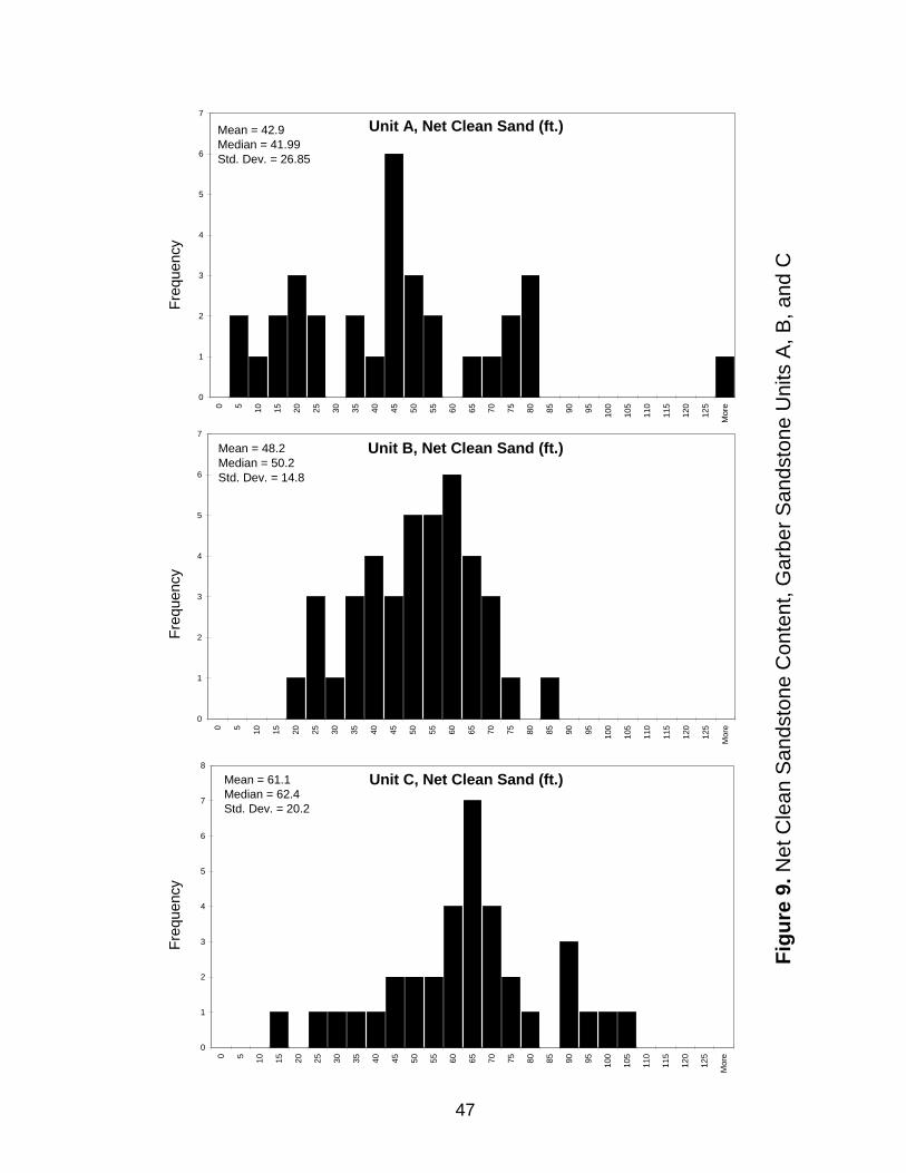
of net clean sand content, percent clean sand, and percent shaly sand for each of the three

main Garber packages were constructed and are presented as Figures 9, 10, and 11,

respectively. In terms of net clean sand thickness (in feet), Unit C was the sandiest,

averaging 61 feet of clean sand per well, and Unit A was the shaliest, averaging 43 feet of

clean sand per well. Units B and C appear to have fairly normal distributions, but Unit A

looks much more irregular. Unit C also has the highest average percent clean sand,

39

averaging 43% clean sand in each well, while Units A and B both average about 40%

clean sand in each well. These percentages are about the same, but the frequency

distributions for each unit look quite different, especially Unit B, which does not appear

to have a normal distribution. Both Units A and B seem to have more samples towards

the low end of the scale than Unit C. Unit A has the highest percent shaly sand,

averaging 51%. Units B and C are similar, averaging 45% and 43%, respectively. Units

A and B have more values on the higher end of the scale than does Unit C. From the

summary statistics and collection of histograms, it appears that in general, Unit C is the

sandiest package and Unit A is the shaliest unit, that is, sand content in the Garber

decreases upward. From visual evaluation of the histograms, it also appears that

normality of the sample population increases with depth. T-tests were not performed to

test for statistical significance.

In her 2005 OSU master’s thesis, Kathy Kenny reports similar results regarding

grain size and stratigraphic interval. She has found that the outcrops lower in the section

are the coarsest-grained, and that grain size decreases upward through the study interval.

These findings independently corroborate the findings based on well logs presented in the

preceding paragraph.

Maps

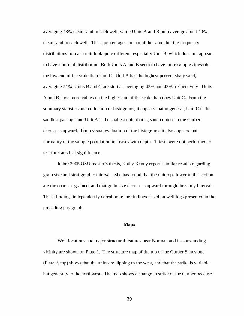
Well locations and major structural features near Norman and its surrounding

vicinity are shown on Plate 1. The structure map of the top of the Garber Sandstone

(Plate 2, top) shows that the units are dipping to the west, and that the strike is variable

but generally to the northwest. The map shows a change in strike of the Garber because

40

of the presence of the Oklahoma City structure to the north of the study area. Also on

Plate 2 is an isopach map of the Garber Sandstone, which shows thickening to the east up

to the outcrop edge.

Several of the maps constructed for this study (shown on Plate 3A) were based on

the total amount of sandstone and shale in each well bore, irrespective of what part of the

section the well penetrated. This was done to identify any trends present over an area for

which continuous units could not be identified. Maps constructed in this manner include

percent sand, percent shale, and percent shaly sand maps, as well as a clean sand to shale

ratio map and a clean sand to shaly sand ratio map. Generally speaking, each of these

maps show a transition from high sand content to low sand content from east to west.

The most predominant and recurring anomalies on these maps are two prominent high-

sand content areas east of Norman and one prominent low-sand content area west of

Norman. Although these maps could have some shortcomings because the thickness of

the sampled interval is decreasing to the west (because of the regional dip), the presence

of recurring anomalies on different maps suggests the observations and interpretations are

valid.

One concern with these maps was due to the increasing depth of penetration into

the Garber-Wellington Aquifer to the east as a result of the westward dip of the strata.

That is, wells to the east of the study area generally contained a thicker section of Garber-

Wellington because the aquifer is dipping to the west. Therefore, it was a possibility that

the eastward increase in sand percentage might actually be an artifact of the mapping

technique, that is, the presence of a sandier interval in the lower Garber in the east that

was not logged in wells to the west. To test whether or not this was the case, a map was

41

constructed of net thickness of clean sand in the upper 300 feet of the Garber. Three-

hundred feet was the approximate minimum thickness of Garber penetrated in the

western wells, and therefore was the thickest interval common to all the wells being used

on the percent lithofacies maps. Since the same trend (decreasing sand content

westward) was detected in the upper 300 feet of Garber in these wells, it seemed

reasonable to conclude that the occurrence of more sandstone to the east was not due

solely to the effects of a lower, sandier interval having not been penetrated in the western

wells.

To investigate the relationship between lithofacies and arsenic distribution, a

bubble map of arsenic concentration was created. This was done by plotting a colored

circle around a well symbol; the radius of each circle is proportional to the arsenic

concentration in that particular well. This is similar to production maps in the petroleum

industry. The bubble map was then drawn on top of the Norman area lithofacies maps,

and the resulting overlay (Plate 3B) was examined to see if high arsenic areas

corresponded to high shale or shaly sand areas, and if low arsenic areas corresponded to

areas high in clean sand content. Although a relationship is visible on all the overlays, it

appears to be strongest on the shaly sand map. Arsenic concentration may be more

closely related to shaly sand content rather that shale or clean sand content because the

mixture of clays and sand grains could result in an aquifer permeable enough to yield

water, yet not permeable enough to permit thorough flushing. There are a few outliers,

particularly to the west, where OU Well #9 has a relatively high arsenic concentration but

is relatively low in shaly sand content. The outliers could be because of secondary

mobilization of the arsenic (Gromadzki, 2004) or due to differences in water chemistry.

42

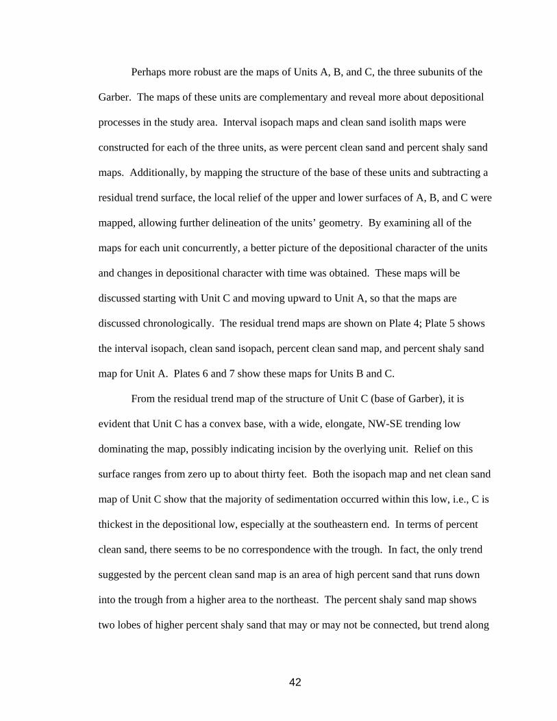
Perhaps more robust are the maps of Units A, B, and C, the three subunits of the

Garber. The maps of these units are complementary and reveal more about depositional

processes in the study area. Interval isopach maps and clean sand isolith maps were

constructed for each of the three units, as were percent clean sand and percent shaly sand

maps. Additionally, by mapping the structure of the base of these units and subtracting a

residual trend surface, the local relief of the upper and lower surfaces of A, B, and C were

mapped, allowing further delineation of the units’ geometry. By examining all of the

maps for each unit concurrently, a better picture of the depositional character of the units

and changes in depositional character with time was obtained. These maps will be

discussed starting with Unit C and moving upward to Unit A, so that the maps are

discussed chronologically. The residual trend maps are shown on Plate 4; Plate 5 shows

the interval isopach, clean sand isopach, percent clean sand map, and percent shaly sand

map for Unit A. Plates 6 and 7 show these maps for Units B and C.

From the residual trend map of the structure of Unit C (base of Garber), it is

evident that Unit C has a convex base, with a wide, elongate, NW-SE trending low

dominating the map, possibly indicating incision by the overlying unit. Relief on this

surface ranges from zero up to about thirty feet. Both the isopach map and net clean sand

map of Unit C show that the majority of sedimentation occurred within this low, i.e., C is

thickest in the depositional low, especially at the southeastern end. In terms of percent

clean sand, there seems to be no correspondence with the trough. In fact, the only trend

suggested by the percent clean sand map is an area of high percent sand that runs down

into the trough from a higher area to the northeast. The percent shaly sand map shows

two lobes of higher percent shaly sand that may or may not be connected, but trend along

43

the same position as the low. Additionally, an elongate area of lower percent shaly sand

rests along the northeast edge of the trough, and trends up onto it, similar to the high

percent clean sand body on the other map. This same geometry occurs on the high area

to the southwest; the percentage of shaly sand decreases as one moves up onto the high

area. These maps show that Unit C first filled in the low area, and that high percent clean

sand and low percent shaly sand do not necessarily coincide with the area of highest net

clean sand or net overall thickness. Perhaps this is because although the main part of the

channel system occupied the trough, the cleanest areas in terms of percent lithofacies

occur mostly on the highs. This may mean that Unit C started out as a deeper water

deposit and by the time the low had been mostly filled up, the environment was more

conducive to cleaner sediments and/or winnowing out of fines.

Relief on the upper surface of Unit C (also the lower surface of Unit B) ranges

from zero to about sixty feet. This surface is characterized by a high that is almost

identical to the position of the low at the base of Unit C. It makes sense that the base of

B would be higher here since it corresponds to the area of highest sedimentation in Unit

C. Furthermore, the low areas at the base of B correspond to the high areas at the base of

C. A low to the southwest in the map area has the highest isopach thickness for Unit B,

again indicating filling in of low areas. However, Unit B is very thin over a low in the

northeast of the map area; this suggests either erosion of Unit B by Unit A, or decreased

sedimentation to the northeast, which would indicate a shift of the main depositional

system to the west. Across the top of the high at the base of the unit, the isopach

thickness of B decreases from west to east, again suggesting decreased sedimentation to

the east. However, the net clean sand map, percent clean sand map, and percent shaly

44

sand map show that the thickest, cleanest sands were deposited in a north-northeast

trending strip that runs from the central high into the northeast low. The percent clean

sand map and net clean sand map also show decreased occurrence of sand to the west of

the map area. Therefore, it appears that total stratigraphic thickness increases to the west,

but clean sand content increases to the east. The percent shaly sand map, similar to the

corresponding map for Unit C, shows that an area of higher percent shaly sand lies

northeast of and adjacent to the area of lower shaly sand content. So for Unit B, it

appears that overall sedimentation rates were higher to the west, but deposition of cleaner

lithofacies was occurring in the eastern part of the mapped area. Perhaps this means that

Unit B first started to fill in the low to the northeast, but the main fairway of

sedimentation began to shift to the west and subsequently spread out over the map area.

The base of Unit A/top of Unit B is very similar to the base of Unit B/top of Unit

C. Relief ranges from zero to about 50 feet. This suggests that the high established by

the lobate feature of Unit C persisted through the section. So, although Unit B is thickest

in the southwest, this area remains a low at the top of B, relative to the central ridge.

Unit A is thickest in the low to the northeast. The thickest portion of Unit A

overlies the thinnest area of Unit B, which is to the northeast and coincides with the

region of greatest sand content in B. The net clean sand, percent clean sand, and percent

shaly sand are all highest in this area also (to the east and northeast). Therefore, it may

be the case that Unit A filled in the low next to the high created by C and perpetuated by

B, because the greatest quantity of sediments and the percent clean sand are greatest in

the low. Unit A is the only unit for which thickest sediment package and cleanest

sediment package are coincident. The residual trend map of the top of Unit A (top of

45

Garber Sandstone) shows a high, with relief up to 20-30 feet. This high corresponds to

the area of thickest sedimentation in Unit A, indicating that the ridge created by Unit C

and also present at the top of Unit B has influenced sedimentation on either side of it. By

the time we move up to the top of Unit A, the highs are located on either side of where

the original trough was, with a depositional low running down the middle.

The well log signatures, maps, and cross sections suggest that the depositional

environment for the Garber Sandstone was fluvial, most likely meandering. This

conclusion has also been reached by Kathy Kenney in her 2005 OSU thesis, in which she

reports outcrop evidence for a meandering fluvial environment. Features she has

observed on outcrops, such as lateral facies changes and compensatory stacking, are also

evident on the cross sections and maps. She has also observed fluvial characteristics such

as point bar deposits and erosional contacts, which are also evident on well log

signatures.

Table 1. Summary statistics for various parameters in OU and Norman water wells. All net thickness values are in feet.

Norman OU Norman OU Norman OUArsenic (ppb) 25.8 34.7 10.7 26.5 43.1 20.8Total Depth (ft.) 679.4 635.4 690.0 629.0 89.4 78.5Net Clean Sand, logged interval 212.8 126.8 215.3 122.2 53.7 33.9Net Clean Sand, Upper 300 ft. 125.9 93.8 114.7 93.7 40.1 28.6Net Clean Sand >4 ft. 193.5 112.0 197.0 116.2 49.2 33.8Net Clean Sand >8 ft. 156.2 91.8 153.9 101.0 48.6 38.8Net Shale 92.2 87.4 97.0 89.0 49.8 39.1

Unit A Interval Thickness 120.0 97.8 103.8 96.0 43.5 12.5Unit A Net Clean Sand 52.7 22.9 47.0 16.2 25.9 17.6Unit A Net Shale 8.4 14.6 5.3 5.8 10.5 17.6Unit A Net Shaly Sand 60.2 58.0 54.1 57.0 29.4 14.4

Unit B Interval Thickness 116.9 148.9 118.5 145.0 18.0 15.3Unit B Net Clean Sand 48.4 42.1 50.7 40.3 14.0 13.9Unit B Net Shale 13.6 33.4 10.4 35.5 10.7 17.6Unit B Net Shaly Sand 54.8 64.3 53.7 63.3 21.8 17.3

Unit C Interval Thickness 139.7 146.5 119.0 142.0 37.3 13.5Unit C Net Clean Sand 59.2 66.7 59.0 67.1 22.2 13.3Unit C Net Shale 16.8 25.5 12.8 24.9 15.1 19.1Unit C Net Shaly Sand 64.0 51.0 65.5 51.1 19.7 12.6

Average Median Standard Deviation

Figure 8. Comparison of Average Values for OU and Norman Water Wells (units are feet except where noted)

0.0

100.0

200.0

300.0

400.0

500.0

600.0

700.0

Ars

enic

(ppb

)

Tota

l Dep

th (f

t.)

Net

Cle

an S

and,

logg

ed in

terv

al

Net

Cle

an S

and,

Upp

er 3

00 ft

.

Net

Cle

an S

and

>4 ft

.

Net

Cle

an S

and

>8 ft

.

Net

Sha

le

Uni

t A In

terv

al T

hick

ness

Uni

t A N

et C

lean

San

d

Uni

t A N

et S

hale

Uni

t A N

et S

haly

San

d

Uni

t B In

terv

al T

hick

ness

Uni

t B N

et C

lean

San

d

Uni

t B N

et S

hale

Uni

t B N

et S

haly

San

d

Uni

t C In

terv

al T

hick

ness

Uni

t C N

et C

lean

San

d

Uni

t C N

et S

hale

Uni

t C N

et S

haly

San

d

Norman WellsOU Wells

46

Unit A, Net Clean Sand (ft.)

0

1

2

3

4

5

6

7

0 5 10 15 20 25 30 35 40 45 50 55 60 65 70 75 80 85 90 95 100

105

110

115

120

125

Mor

e

Mean = 42.9Median = 41.99Std. Dev. = 26.85

Unit B, Net Clean Sand (ft.)

0

1

2

3

4

5

6

7

0 5 10 15 20 25 30 35 40 45 50 55 60 65 70 75 80 85 90 95 100

105

110

115

120

125

Mor

e

Mean = 48.2Median = 50.2Std. Dev. = 14.8

Unit C, Net Clean Sand (ft.)

0

1

2

3

4

5

6

7

8

0 5 10 15 20 25 30 35 40 45 50 55 60 65 70 75 80 85 90 95 100

105

110

115

120

125

Mor

e

Mean = 61.1Median = 62.4Std. Dev. = 20.2

Figu

re 9

. Net

Cle

an S

ands

tone

Con

tent

, Gar

ber S

ands

tone

Uni

ts A

, B, a

nd C

Freq

uenc

yFr

eque

ncy

Freq

uenc

y

47

Unit A, Percent Clean Sand

0

1

2

3

4

5

6

7

0

0.05 0.

1

0.15 0.

2

0.25 0.

3

0.35 0.

4

0.45 0.

5

0.55 0.

6

0.65 0.

7

0.75 0.

8

0.85 0.

9

0.95 1

Mor

e

Mean = 0.404Median = 0.426Std. Dev. = 0.201

Unit B, Percent Clean Sand

0

1

2

3

4

5

6

7

0

0.05 0.1

0.15 0.2

0.25 0.3

0.35 0.4

0.45 0.5

0.55 0.6

0.65 0.7

0.75 0.8

0.85 0.9

0.95 1

Mor

e

Mean = 0.398Median = 0.389Std. Dev. = 0.138

Unit C, Percent Clean Sand

0

1

2

3

4

5

6

7

8

9

0

0.05 0.1

0.15 0.2

0.25 0.3

0.35 0.4

0.45 0.5

0.55 0.6

0.65 0.7

0.75 0.8

0.85 0.9

0.95 1

Mor

e

Mean = 0.431Median = 0.466Std. Dev. = 0.124

Figu

re 1

0.P

erce

nt C

lean

San

dsto

neC

onte

nt, G

arbe

r San

dsto

ne U

nits

A, B

, and

C

Freq

uenc

yFr

eque

ncy

Freq

uenc

y

48

Unit A, Percent Shaly Sand

0

1

2

3

4

5

6

0

0.05 0.1

0.15 0.2

0.25 0.3

0.35 0.4

0.45 0.5

0.55 0.6

0.65 0.7

0.75 0.8

0.85 0.9

0.95 1

Mor

e

Mean = 0.510Median =0.525Std Dev = 0.150

Unit B, Percent Shaly Sand

0

1

2

3

4

5

6

7

8

0

0.05 0.

1

0.15 0.

2

0.25 0.

3

0.35 0.

4

0.45 0.

5

0.55 0.

6

0.65 0.

7

0.75 0.

8

0.85 0.

9

0.95 1

Mor

e

Mean = 0.452Median =0.439Std Dev = 0.133

Unit C, Percent Shaly Sand

0

2

4

6

8

10

12

14

0

0.05 0.

1

0.15 0.

2

0.25 0.

3

0.35 0.

4

0.45 0.

5

0.55 0.

6

0.65 0.

7

0.75 0.

8

0.85 0.

9

0.95 1

Mor

e

Mean = 0.433Median =0.433Std Dev = 0.100

Figu

re 1

1.P

erce

nt S

haly

San

dsto

neC

onte

nt, G

arbe

r San

dsto

ne U

nits

A, B

, and

C

Freq

uenc

yFr

eque

ncy

Freq

uenc

y

49

50

Large Scale Cross Sections

The location of these cross section lines, X-X’ and Y-Y’, are shown on Figure 12

as well as Plate 8. Structural cross section X-X’ shows the regional dip in the east-west

direction, south of the Oklahoma County/Cleveland County line. On this cross section,

the top of the Garber dips to the west at about 30 feet per mile, and the underlying

surfaces have similar dips. The inferred Garber-Wellington contact on the east side of

the cross section is because of a lack of wells for which this contact was logged in the

eastern half of Cleveland County. The cross section also shows the facies transition of

the Herington Limestone to a shale section.

Structural cross section Y-Y’ shows the regional dip in a north-south direction in

the western part of Cleveland County and southern Oklahoma County. The cross section

shows that the beds are striking more or less north-south in Oklahoma County, and they

begin to dip slightly to the south in northern Cleveland County, before flattening out just

north of Norman and then rising slightly between Norman and Noble. The cross section

suggests the presence of a subtle depression or low area between the north line of T9N

R3W and the Noble vicinity.

Small Scale Cross Sections and Well Log Response Patterns

The discussion of the small scale cross sections (A-A’ through H-H’) consists of

some general information about each cross section, such as a brief description of the

orientation of the cross section line and some of the features seen on that particular cross

section. The location of these cross section lines can be found on Figure 13, and also on

XX’

Y

Y’

XX’

Y

Y’

Figure 12. Map showing location of cross sections X-X’ and Y-Y’

51

Figure 13. Map Showing location of cross sections A-A’ through H-H’

52

53

Plate 8. The cross sections can be found on Plates 10, 11, 12, and 13.

Cross section A-A’ runs approximately east-west, except for a portion of the line

which runs more north-south. A-A’ is hung stratigraphically on the top of the Garber,

and is tied into cross section B-B’ by well N5. Among the characteristics seen on this

cross section are fining upward intervals which probably represent point bar deposits.

Also seen are relatively clean, thick sandstones developing shale breaks and grading into

thinly bedded sands and shales. Individual sandstones on well logs can be as thick as

fifty feet. Also present is a continuous sandstone at the base of Unit B. This sandstone is

blocky in places and is about thirty feet thick, except in the two westernmost wells, where

it is thinner. This sandstone is present in quite a few wells used in the cross section.

Figure 14 is a detail from Cross Section H-H’ showing the typical log signature of this

sandstone. Figure 15 is a detail from Cross Section D-D’ showing typical gradation of

shale and blocky sandstones into more thinly bedded sandstones.

Cross section B-B’ is a north-south line, hung structurally (datum = MSL)

because the top of the Garber is not found on some of the logs. The section is more or

less on strike in the northern end of the line, and the units begin to dip to the south

towards the southern end. This cross section shows the gradation of thick sandstones into

fining upward series, and the development of thin shale breaks within thick sands.

Truncation is also present, as are stacked fining upward intervals.

Cross section C-C’ is hung on the top of the Garber and runs in an east-west

direction. Except for the two end wells, the wells in this cross section occur in very

OU3A NC2A NC1 N21

UNIT B

UNIT B

NT4 N35 N36

Figure 14. Detail of cross section H-H’, showing the persistent sandstone at the base of Garber Unit B.

Figure 15. Detail of cross section D-D’, showing the typical lateral gradation of sandstone to shale in the Garber. Note the fining-upward character in well N35.

300 ft. 1800 ft.

960 ft. 1640 ft. 7600 ft.

54

55

closely spaced pairs. The major unit boundaries on this cross section are sometimes

rather subtle, but the author believes the boundaries are in the correct position since they

were carried through from other cross sections where they are more apparent. Similar to

cross sections A-A’ and B-B’, this section shows thick sandstones grading into more

thinly bedded sandstones and shales over distances of several hundred feet, and the

interbedded sandstones and shales grading into fining upward intervals. Persistent

sandstone units are present at the top of Unit A and at the base of Unit B. A thick shale

unit is also present in Unit B.

Cross section D-D’ is a structural cross section, with the top of the Garber

projected across several wells where it cannot be seen on the logs. The base of the

Garber is relatively flat lying. This cross section is more or less a loop, going north,

turning east, and then heading back south, as it ties into cross section C-C’ at both ends.

Some of the features seen on this cross section include stacked sandstones, rapid

thickening and thinning of shales, and once again, lateral gradation of thick sandstones

into interbedded sandstone and shale, over distances of less than a mile. Unit B contains

a continuous sandstone at its base.

Cross section E-E’ is a stratigraphic section hung on the top of the Garber; this

cross section goes through the two NOTS wells in the Norman area, NOTS 7 and 7A.

These two wells are very close together, and the top of the Garber can be seen easily on

both logs, as well as the upper and lower surfaces of Unit B. Only two wells in this cross

section penetrate the base of the Garber. E-E’ is a north-south cross section, connecting

cross sections A-A’, F-F’, and H-H’. This cross section exhibits the characteristic lateral

gradation of sandstone to shale seen on each of the preceding cross sections, as well as

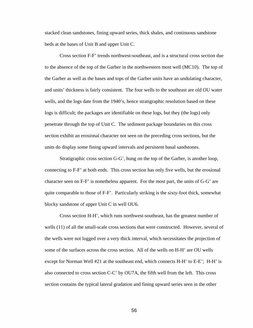
56

stacked clean sandstones, fining upward series, thick shales, and continuous sandstone

beds at the bases of Unit B and upper Unit C.

Cross section F-F’ trends northwest-southeast, and is a structural cross section due

to the absence of the top of the Garber in the northwestern most well (MC10). The top of

the Garber as well as the bases and tops of the Garber units have an undulating character,

and units’ thickness is fairly consistent. The four wells to the southeast are old OU water

wells, and the logs date from the 1940’s, hence stratigraphic resolution based on these

logs is difficult; the packages are identifiable on these logs, but they (the logs) only

penetrate through the top of Unit C. The sediment package boundaries on this cross

section exhibit an erosional character not seen on the preceding cross sections, but the

units do display some fining upward intervals and persistent basal sandstones.

Stratigraphic cross section G-G’, hung on the top of the Garber, is another loop,

connecting to F-F’ at both ends. This cross section has only five wells, but the erosional

character seen on F-F’ is nonetheless apparent. For the most part, the units of G-G’ are

quite comparable to those of F-F’. Particularly striking is the sixty-foot thick, somewhat

blocky sandstone of upper Unit C in well OU6.

Cross section H-H’, which runs northwest-southeast, has the greatest number of

wells (11) of all the small-scale cross sections that were constructed. However, several of

the wells were not logged over a very thick interval, which necessitates the projection of

some of the surfaces across the cross section. All of the wells on H-H’ are OU wells

except for Norman Well #21 at the southeast end, which connects H-H’ to E-E’; H-H’ is

also connected to cross section C-C’ by OU7A, the fifth well from the left. This cross

section contains the typical lateral gradation and fining upward series seen in the other

57

cross sections, as well as a thick shale unit and a thick, continuous sandstone at the base

of Unit B. There is also a prominent coarsening upward interval in OU7A in upper Unit

B.

All of the cross sections exhibit several instances of fining upward intervals,

which are probably point bar deposits. Many of these deposits are incomplete; that is, the

upper part of the point bar deposits have been removed or were never deposited. All of

the cross sections also show prominent lateral gradation of thick, clean sandstones into

thinner, interbedded sandstones and shales and also into the point bar deposits. There are

few coarsening upward sequences. Frequently, especially in Unit B, there is a relatively

clean sandstone at the base of a unit that is continuous across an entire cross section.

This suggests that water depth and energy was fairly consistent at the beginning of

deposition of these units. These characteristics suggest that the rocks of the Garber

Sandstone are similar to the “meanderbelt facies” discussed in the paper by Hall (1976).

From the literature, it appears that Norman is situated in an area of the aquifer

with lower sand content relative to areas to its north and east. Burton and Wood assert

that the sandstone to shale ratio is highest in northeastern Cleveland County and

decreases to the southwest, while other authors maintain that sand content is highest in

central Oklahoma County and decreases outward in all directions. In the immediate

Norman area, however, there are trends that suggest the presence of areas of locally low

and high sand content. In general, clean sand seems to be more abundant to the east and

at deeper intervals within the Garber (i.e., Unit C is sandier than Units A and B- refer to

Figures 9, 10, and 11). The areal variations are probably more significant than the

vertical variations, because it is not uncommon to find a thick, clean sandstone at any

58

given interval within the Garber. That is, although sand content may increase from Unit

A downward, the difference is not very large from one unit to the next when compared

with the differences from one well location to the next. Neither does it appear that

arsenic occurrence can be linked to any one unit or individual sediment layer, since they

usually grade into something else relatively rapidly. Therefore, it is recommended that

wells be drilled in areas with high clean sand and low shaly sand (Figure 16).

59

VI.

CONCLUSIONS AND SUGGESTIONS FOR FUTURE WORK

The primary source of data for this study was well logs, which were used to

construct various maps and cross sections. After examining this data, the following

conclusions can be drawn.

1.) The Garber Sandstone in Cleveland County ranges from about 400-600 feet thick,

and dips to the west at approximately 35 feet per mile, except where the regional

dip is influenced by deeper structure

2.) Sediment packages exist within the Garber Sandstone that can be correlated from

well to well over moderate distances. Three locally continuous sediment

packages have been identified in the Garber (Units A, B, and C).

3.) Similar to what is seen in outcrops, individual sandstone bodies within these

packages pinch out or grade laterally into shale over shorter distances. Clean

sandstone units often grade into more thinly bedded sandstone and shale, or into

fining upward intervals.

4.) The maps of Units A, B, and C suggest that the dominant style of deposition has

resulted in the formation of depositional highs followed by increased

sedimentation in the adjacent low areas.

5.) Variations in arsenic distribution coincide reasonably well with lithofacies,

especially shaly sandstone, though there are some outliers.

60

One focus for future work could be to attempt linking arsenic distribution with

various parts of the fluvial system, such as overbank deposits, channel mouth bars, etc.

There is also potential for this work to be carried northward into Oklahoma County,

especially the Tinker Air Force Base area. The same units mapped here (A, B, and C)

may not be present, but most likely similar or equivalent units can be identified and

mapped. Regarding more detailed stratigraphic analysis, chemostratigraphy and FMI and

micro-resistivity logs would be extremely informative but immediate availability is

unlikely due to analytical cost. However, detailed studies of well log signatures could be

used to reconstruct the various parts of the channel system in terms of their

paleogeomorphology.

Figure 16. Potentially high and low arsenic zones in the Norman area

61

62

REFERENCES CITED

Aurin, F.L., H.G. Officer, and C.N. Gould, 1926, The Subdivision of the Enid Formation: AAPG Bulletin, v. 10, no. 8, p. 786-799.

Dott, R.H., 1932, Lower Permian Correlations in Cleveland, McClain, and Garvin

Counties, Oklahoma: AAPG Bulletin, v. 16, no. 2, p. 119-134. Patterson, J.M., 1933, Permian of Logan and Lincoln Counties, Oklahoma: AAPG

Bulletin, v. 17, no. 3, p. 241-253. Foley, L.L., 1934, Tectonics of Oklahoma City Anticline: AAPG Bulletin, v. 18, no. 2,

p. 251-262 Green, D.A., 1936, Permian and Pennsylvanian Sediments Exposed in Central and West-

Central Oklahoma: AAPG Bulletin, v. 20, no. 11, p. 1454-1475. Tanner, W.F., 1959, Permo-Pennsylvanian Paleogeography of Part of Oklahoma: Journal

of Sedimentary Petrology, v. 29, no. 3, p. 326-335. Gatewood, L.E., 1968, Oklahoma City Field – Anatomy of a Giant: AAPG Bulletin, v.

52, no. 3, p. 528. Wood, P.R., and L.C. Burton, 1968, Ground-Water Resources in Cleveland and

Oklahoma Counties, Oklahoma: Oklahoma Geological Survey, Norman, OK, Circular 71, 75 p.

Hall, D.H., 1976, Hydrogeologic Significance of Depositional Systems and Facies in

Lower Cretaceous Sandstones, North-Central Texas: Bureau of Economic Geology, The University of Texas at Austin, Geologic Circular 76-1, 29 p.

Mosier, E.L., and J.H. Bullock, 1988, Review of the General Geology and Solid-Phase

Geochemical Studies in the Vicinity of the Central Oklahoma Aquifer: U.S. Geological Survey, Oklahoma City, OK, Circular 1019, 22 p.

Breit, G.N, C. Rice, K. Esposito, and J.L. Schlottmann, 1990, Mineralogy and

Petrography of Permian Rocks in the Central Oklahoma Aquifer: U.S. Geological Survey, Oklahoma City, OK, Open-File Report 90-678, 50 p.

63

Schlottmann, J.L., and R.A. Funkhouser, 1991, Chemical Analyses of Water Samples and Geophysical Logs from Cored Test Holes Drilled in the Central Oklahoma Aquifer, Oklahoma: U.S. Geological Survey, Oklahoma City, OK, Open-File Report 91-464, 58 p.

Christenson, S., 1992, Geohydrology and Ground-Water Flow Simulation of the

Central Oklahoma Aquifer [abstract], in S. Christenson and L. Carpenter, eds., Ground-Water Quality of the Central Oklahoma (Garber-Wellington) Aquifer Conference: Proceedings, February 20, 1992: U.S. Geological Survey, Oklahoma City, OK, Open-File Report 92-116, p. 5-6.

Breit, G.N., 1998, The Diagenetic History of Permian Rocks in the Central Oklahoma

Aquifer, in S. Christenson and J.S. Havens, eds., Ground-Water-Quality Assessment of the Central Oklahoma Aquifer, Oklahoma: Results of Investigations: U.S. Geological Survey, Oklahoma City, OK, Water-Supply Paper 2357-A, p. 45-61.

Schlottmann, J.L., E.L. Mosier, and G.N. Breit, 1998, Arsenic, Chromium, Selenium, and

Uranium in the Central Oklahoma Aquifer, in S. Christenson and J.S. Havens, eds., Ground-Water-Quality Assessment of the Central Oklahoma Aquifer, Oklahoma: Results of Investigations: U.S. Geological Survey, Oklahoma City, OK, Water-Supply Paper 2357-A, p. 119-179.

Roberts, J., 2001, Characterizing and Mapping the Regional Base of an Underground

Source of Drinking Water in Central Oklahoma Using Open-Hole Geophysical Logs and Water Quality Data: Enercon Services, Inc., Oklahoma City, OK, unpublished work, 91 p.

Gromadzki, G., 2004, Outcrop-based gamma-ray characterization of arsenic-bearing lithofacies in the Garber-Wellington Formation, Central Oklahoma Aquifer (COA), Cleveland County, Oklahoma: Unpublished M.S. Thesis, Oklahoma State

University, 150 p.

64

APPENDICES

65

APPENDIX A

WELL HEADER DATA

Well Header Information

Well Label Well Name Latitude Longitude Township Range Section Quarter County Datum Elevation2 Washington School Test Well #2 35.212736 -97.372814 9N 2W 35 SE NE Cleveland 11305 Griffin Memorial Hospital #5 35.226475 -97.418133 9N 2W 28 SW SE NW Cleveland 119930 NormanWWNW36th No info. Cleveland31 NormanWW#8A No info. Cleveland32 Ada Flemming #A-1 35.370688 -97.207287 10N 1E 4 C SW SE NW Cleveland 119533 Hirsche #1 35.376271 -97.247101 10N 1E 6 NW NW NW Cleveland 115534 Wodkins #1 35.359703 -97.196162 10N 1E 9 SE NE NE Cleveland 122535 Coley #1 35.353341 -97.183996 10N 1E 10 C NW SE Cleveland 119136 R. E. Wilson #1 35.343183 -97.158594 10N 1E 13 NW SW NW Cleveland 116037 Foster 'B' #1 35.346892 -97.162948 10N 1E 14 NW NE NE Cleveland 116238 Franklin #1 35.346088 -97.192842 10N 1E 15 NW NW Cleveland 123839 State Land #1 35.342593 -97.206033 10N 1E 16 C SE NW Cleveland 120940 Barton #1 35.323408 -97.187187 10N 1E 22 SE NE SW Cleveland 117741 Wilson Estate #1 35.317953 -97.182632 10N 1E 27 NE NW NE Cleveland 114542 Wilson #1 35.310851 -97.202525 10N 1E 28 NW NW SE Cleveland 114243 Gunter #1 35.307236 -97.229131 10N 1E 29 NW SW SW Cleveland 114944 Parr #1 35.299015 -97.201249 10N 1E 33 C SW NE Cleveland 118545 Helen Anderson #1 35.363657 -97.24866 10N 1W 1 SE SE SE Cleveland 117646 Pringle #1 35.363677 -97.26823 10N 1W 2 SW SE SE Cleveland 114247 Maree Lewinsohn #1 35.354666 -97.297006 10N 1W 10 Cleveland 121548 Northcott #1 35.358329 -97.270445 10N 1W 11 NE SW NE Cleveland 116749 Hayes #1 35.334623 -97.262001 10N 1W 13 SE SW SW Cleveland 115050 Little #1 35.320367 -97.29261 10N 1W 22 SE SE SW Cleveland 118751 Owenbey #1 35.325788 -97.266009 10N 1W 23 NE NE SE Cleveland 118852 Lucas #1 35.311201 -97.279314 10N 1W 26 NE NW SW Cleveland 117353 Hall #1 35.306003 -97.33696 10N 1W 30 SE SE SE Cleveland 115854 Zimmerman #1 35.291566 -97.34811 10N 1W 31 SW SE SW Cleveland 107755 Sublett #1 35.302394 -97.325982 10N 1W 32 SW NW NE Cleveland 114756 Quiett #1 35.30205 -97.266129 10N 1W 35 SE NE NE Cleveland 113357 Conley #1 35.367439 -97.378718 10N 2W 2 SW NW SE Cleveland 118458 Rice #2 35.374825 -97.400442 10N 2W 3 SW NE NW Cleveland 126059 Shroyer #1 35.360343 -97.39169 10N 2W 10 SW NE NE Cleveland 119560 State #5 35.33597 -97.412443 10N 2W 16 NE SW SW SE Cleveland 116461 Lindsay #3 35.343204 -97.434638 10N 2W 17 C SE NW Cleveland 123564 Cook #1 35.307116 -97.372952 10N 2W 26 C SE SE Cleveland 115765 Young #4 35.306084 -97.433522 10N 2W 29 SE SE SW Cleveland 116066 Keller #1 35.292555 -97.412593 10N 2W 33 SW SE Cleveland 115567 Fox #1 35.297063 -97.395946 10N 2W 34 NW NW SE Cleveland 111568 Shelburg #1 35.292546 -97.386251 10N 2W 35 C SW SW Cleveland 111269 State #36-1 35.304256 -97.358597 10N 2W 36 NE NW NE Cleveland 110870 School Land #1-B 35.297027 -97.365239 10N 2W 36 NW NE SW Cleveland 1162

66

Well Label Well Name Latitude Longitude Township Range Section Quarter County Datum Elevation75 Nail #1 35.350419 -97.474732 10N 3W 12 SW SW Cleveland 125776 Steinmeyer #1 35.339621 -97.465846 10N 3W 13 C NW SE Cleveland 121082 Kysela #4 35.328703 -97.549864 10N 3W 19 C SE NE Cleveland 121383 Miller #1 35.328858 -97.518801 10N 3W 21 SW NE Cleveland 122984 Perry Jury #1 35.317903 -97.466844 10N 3W 25 W/2 NW NE Cleveland 118985 Sullivan #2 35.317945 -97.50987 10N 3W 27 NW NW Cleveland 121789 McBride #1 35.350099 -97.646805 10N 4W 8 SE SW Cleveland 127791 SE Wheatland WSW 35.362037 -97.575388 10N 4W 12 NE NE NW Cleveland 120892 Test Hole #1 35.347245 -97.659044 10N 4W 18 NE NW NE Grady 131293 Russell Butler #3 35.328534 -97.598457 10N 4W 23 C SW NW Cleveland 122096 Foster #1 35.276327 -97.162719 9N 1E 2 SW SE SE Cleveland 113697 Hoover #1 35.281928 -97.195713 9N 1E 4 NE NE SE Cleveland 113798 Williams #1 35.27407 -97.232008 9N 1E 7 NE NE Cleveland 105899 Go-do-pea-se #1 35.262112 -97.195551 9N 1E 9 SE SE SE Cleveland 1107100 Rookstool #1 35.273727 -97.192374 9N 1E 10 C NW NW Cleveland 1138101 Wilson #1 35.273593 -97.152742 9N 1E 12 C NE NW Cleveland 1051102 Pah Koh Nay #1 35.256309 -97.158243 9N 1E 13 NW SW NW Cleveland 1118103 Citizens Nat'l Bank #1 35.247451 -97.192372 9N 1E 15 C S/2 SW SW Cleveland 1110104 Citizens Nat'l Bank #A-1 35.253066 -97.195437 9N 1E 16 C NE NE SE Cleveland 1138105 Godopease #1 35.259393 -97.218637 9N 1E 17 C NW NE Cleveland 1141106 Benard #1 35.252214 -97.24085 9N 1E 18 C NE SW Cleveland 1026107 Little Axe School Dist. #4 35.244048 -97.195393 9N 1E 21 SE NE NE Cleveland 1100108 Warmack #1 35.233206 -97.204243 9N 1E 21 SE SE SW Cleveland 1071109 White #2 35.244852 -97.187945 9N 1E 22 C E NE NW Cleveland 1037110 Mack #1 35.236537 -97.144964 9N 1E 24 SW NE SE Cleveland 1049111 Essary #1 35.230207 -97.152629 9N 1E 25 C NE NW Cleveland 1107112 Little Fish Unit #1 35.220268 -97.155947 9N 1E 25 NE SW SW Cleveland 1041113 Joe Brendle #1 35.222143 -97.160403 9N 1E 26 SE NE SE Cleveland 1086114 Little Jim #2 35.227565 -97.191302 9N 1E 27 NE SW NW Cleveland 1037115 Edna Hall #1 35.230295 -97.196498 9N 1E 28 C NE NE Cleveland 1026116 Goodin #1 35.207894 -97.213073 9N 1E 32 SE NE SE Cleveland 1041117 King #1 35.207668 -97.208744 9N 1E 33 SE NW SW Cleveland 992118 Austin Estate #1 35.213078 -97.18683 9N 1E 34 NE SE NW Cleveland 992119 Billy Williams #1 35.213058 -97.166553 9N 1E 35 200' W of C N/2 SW NE Cleveland 1049120 McCalmon #1 35.204738 -97.152585 9N 1E 36 C SE SW Cleveland 980121 Banning #1 35.205642 -97.142632 9N 1E 36 NE SE SE Cleveland 980122 Le Master #1 35.284259 -97.292689 9N 1W 3 SE SE NW Cleveland 1179123 Blackburn #1 35.282591 -97.33034 9N 1W 5 NW NE SW Cleveland 1100124 King #1 35.286205 -97.343428 9N 1W 6 NW SW NE Cleveland 1116125 Maddox #1 35.275283 -97.338933 9N 1W 7 NW NE NE Cleveland 1067126 Johnson #1 35.273476 -97.328045 9N 1W 8 SE NE NW Cleveland 1065127 Kelley #1 35.26785 -97.272856 9N 1W 11 NW NW SE Cleveland 1173128 Titus McCoy #1 35.270561 -97.24983 9N 1W 12 SE NE Cleveland 1162

67

Well Label Well Name Latitude Longitude Township Range Section Quarter County Datum Elevation129 McCoy #1 35.254995 -97.248532 9N 1W 13 SE SE NE Cleveland 1123130 Nora Todd #1 35.253574 -97.317035 9N 1W 16 NW NW SW Cleveland 1060131 Forrest Mouser #6 35.25172 -97.319191 9N 1W 17 SE NE SE Cleveland 1118132 Matlock #1 35.256238 -97.346678 9N 1W 18 SE NW Cleveland 1117133 Smith #1 35.23903 -97.347819 9N 1W 19 NW NE SW Cleveland 1173134 R.E. Connelly #1 35.23903 -97.321359 9N 1W 20 NW NE SE Cleveland 1072135 Briggs #1 35.239021 -97.312597 9N 1W 21 NW NE SW Cleveland 1044136 Rohart #1 35.246251 -97.290574 9N 1W 22 NW NW NE Cleveland 1101137 Brehm #1 35.240739 -97.268573 9N 1W 23 SW SE NE Cleveland 1118138 Wilson #1 35.241474 -97.262914 9N 1W 24 C SW NW Cleveland 1155139 Walker #1 35.23152 -97.261899 9N 1W 25 NE NW NW Cleveland 1096140 Clark #1 35.231699 -97.266227 9N 1W 26 NE NE NE Cleveland 1073141 Otto Heims #1 35.228084 -97.290382 9N 1W 27 NW SW NE Cleveland 1184142 Birkhead #1 35.231799 -97.317019 9N 1W 28 NW NW NW Cleveland 1138143 Schonwald #1 35.223699 -97.320211 9N 1W 29 NE SE Cleveland 1144144 Russell #1 35.219124 -97.347704 9N 1W 30 SW SE SW Cleveland 1193145 Lula Vaughn #1 35.212766 -97.350849 9N 1W 31 C SW NW Cleveland 1154146 M.B. Fulkerson #1 35.211712 -97.268317 9N 1W 35 SW SE NE Cleveland 1071147 Holstein #1 35.209905 -97.261896 9N 1W 36 NE NW SW Cleveland 1104148 Nelson #1 35.282605 -97.356382 9N 2W 1 NW NE SE Cleveland 1106149 Williams #B-1 35.28527 -97.399295 9N 2W 3 C SE NW Cleveland 1145150 Kuhlman #1 35.281656 -97.39044 9N 2W 3 C NE SE Cleveland 1090151 Jennings #1 35.278955 -97.418126 9N 2W 4 NW SE SW Cleveland 1146154 Lessly #2-A 35.266349 -97.4093 9N 2W 9 SW NE SE Cleveland 1134156 Oliphant #1 35.27177 -97.389449 9N 2W 10 NE SE NE Cleveland 1142161 Strong #1 35.259847 -97.364175 9N 2W 13 C NE NW Cleveland 1148162 Ray Howell #1 35.259839 -97.377387 9N 2W 14 C NW NE Cleveland 1169163 Hansmeyer #1 35.253514 -97.387345 9N 2W 14 NW NW SW Cleveland 1179167 Boggs #1 35.253592 -97.40718 9N 2W 16 NE NE SE Cleveland 1198170 Rucker #1 35.249136 -97.430258 9N 2W 17 C SW SE Cleveland 1186171 Norman Well #2-A 35.241716 -97.39038 9N 2W 22 SE NE Cleveland 1124172 Klement #1 35.240841 -97.358602 9N 2W 24 SE SW NE Cleveland 1163173 Graves #1 35.239034 -97.363028 9N 2W 24 NE NE SW Cleveland 1177174 Boesken #1 35.227277 -97.394742 9N 2W 27 SW NE Cleveland 1181178 Core Hole #23 35.203982 -97.386049 9N 2W 35 C SL SW SW Cleveland 1199179 ACOG MW OK-3 35.279176 -97.482331 9N 3W 2 NE SW SE Cleveland 1170180 Gross #1 35.275471 -97.528528 9N 3W 9 NW NW NW Cleveland 1142181 OU Naval Base Well #7 35.250124 -97.464675 9N 3W 13 NE SW SE Cleveland 1160182 Helen Hamm #1 35.248218 -97.504316 9N 3W 15 SE SE SW Cleveland 1188184 OU Naval Base Well #6 35.246503 -97.462421 9N 3W 24 NW NE NE Cleveland 1175185 Westport Golf Club Test #1 35.22746 -97.483306 9N 3W 26 SW NE Cleveland 1155192 EW Harris #1 35.3080336 -97.5396357 10N 3W 29 NE SE SW Cleveland 1190193 Test Well #1 35.3015374 -97.5961615 10N 4W 35 NW Cleveland 1190

68

Well Label Well Name Latitude Longitude Township Range Section Quarter County Datum Elevation209 OU Navy Well #5 35.2537747 -97.4689342 9N 3W 13 NE NE SW Cleveland 1170215 Cox #1 35.19012 -97.254069 8N 1W 1 C S/2 SW SE Cleveland 1132216 Stanford #1 35.202904 -97.277159 8N 1W 2 NW NE NW Cleveland 1150217 Sullivant #1 35.202785 -97.308077 8N 1W 4 NW NW NE Cleveland 1118218 Hoffman #2 35.193654 -97.319049 8N 1W 5 SE NE SE Cleveland 1124219 Brown #1 35.175675 -97.345358 8N 1W 7 SE SE SW Cleveland 1130220 Ralph Caddell #1 35.187421 -97.333278 8N 1W 8 NW NW Cleveland 1136221 H. Berman #2 35.177586 -97.297192 8N 1W 10 NE SW SW Cleveland 1179222 Deaver #1 35.180297 -97.267207 8N 1W 11 NE SE Cleveland 1108223 Witt #1 35.166686 -97.274909 8N 1W 14 NE NE SW Cleveland 1140224 F. Cook Jr. #2 35.170411 -97.288262 8N 1W 15 1650 SNL, 1650 WEL Cleveland 1192225 Black #1 35.172959 -97.350821 8N 1W 18 NW NW Cleveland 1141226 Cities Service Oil Company #1 35.159523 -97.283964 8N 1W 22 85' W NE NE NE Cleveland 1165227 Ellis #1 35.152128 -97.259665 8N 1W 24 NW NE SW Cleveland 1180228 Demand #1 35.14314 -97.290403 8N 1W 27 SW NW NE Cleveland 1246229 Schock #1 35.123067 -97.308135 8N 1W 33 NW NW SE Cleveland 1189230 Patterson #1 35.125712 -97.263106 8N 1W 36 SW NW Cleveland 1232231 Core Hole #22 35.195607 -97.369573 8N 2W 1 NW NW SW Cleveland 1145232 Core Hole #24 35.191341 -97.403569 8N 2W 3 SW SW Cleveland 1183235 Core Hole #19 35.176725 -97.381733 8N 2W 11 SE SW Cleveland 1156236 Valouch #1 35.173116 -97.386153 8N 2W 14 NW NW Cleveland 1184237 Core Hole #20 35.173239 -97.394839 8N 2W 15 NW NE Cleveland 1177238 Tullius #4 35.169753 -97.417805 8N 2W 16 1990 FNL, 1770 FWL Cleveland 1175239 Core Hole #18 35.151457 -97.40382 8N 2W 22 NW SW Cleveland 1100241 Taylor #1 35.157782 -97.380717 8N 2W 23 SE NE NW Cleveland 1167243 Core Hole #16 35.151361 -97.368559 8N 2W 24 NW SW Cleveland 1183245 Core Hole #15 35.140489 -97.368557 8N 2W 25 SW NW Cleveland 1193246 Core Hole #13 35.131446 -97.393086 8N 2W 27 C SL SE Cleveland 1133250 Hall Park Well #4 35.238609 -97.414263 9N 2W 21 SW NW NW SE Cleveland 1228257 Noble Pollack #1 35.1149944 -97.3159557 7N 1W 4 NW NW Cleveland 1100GS7 NOTS 7 35.2208333 -97.4286111 Cleveland 1172GS7A NOTS 7A 35.2208333 -97.4283333 Cleveland 1172M21 City of Moore Well #21 35.3207275 -97.51096 10N 3W 22 SW SW SW Cleveland 1210M22 City of Moore #22 35.303515 -97.4746 10N 3W 36 NW NW Cleveland 1215M23 City of Moore Well #23 35.3206462 -97.4778247 10N 3W 23 SE SE SE Cleveland 1225M24 City of Moore Well #24 35.332466 -97.4614039 10N 3W 24 NE NE Cleveland 1199M26 City of Moore Well #26 35.3690343 -97.4975738 10N 3W 3 SE NW NE SE Cleveland 1307M36 City of Moore #36 35.346818 -97.44802 10N 2W 18 C NW NE Cleveland 1245MC1A OU MC Well #1-A 35.2048257 -97.4401572 9N 2W 31 SE SE Cleveland 1163MC2A OU MC Well #2-A 35.2048777 -97.4378563 9N 2W 32 SE SW SW Cleveland 1152MC3A OU MC Well #3A 35.2101285 -97.4422384 9N 2W 31 NE NE SE Cleveland 1175MT1 City of Moore #1 Test Hole 35.364055 -97.462546 10N 3W 1 SW SE SE Cleveland 1275MT2 City of Moore #2 Test Hole 35.335072 -97.451343 10N 2W 18 SE SE SW Cleveland 1198

69

Well Label Well Name Latitude Longitude Township Range Section Quarter County Datum ElevationMTA2 City of Moore Test Well #A-2 35.361392 -97.492263 10N 3W 11 NW NW Cleveland 1280MTB City of Moore Test Well B 35.33969 -97.483493 10N 3W 14 NW SE Cleveland 1230Mu10 City of Mustang Well #10 35.340573 -97.5288416 10N 3W 16 NW NW SW Cleveland 1208Mu11 City of Mustang #11 35.334789 -97.521578 10N 3W 16 SE SE SE SW Cleveland 1217Mu13 City of Mustang #13 35.347731 -97.555403 10N 3W 18 NW NW NE Cleveland 1205Mu2 City of Mustang M-II 35.335273 -97.533304 10N 3W 17 Cleveland 1200Mu9 City of Mustang #9 35.344246 -97.531078 10N 3W 17 NE SE NE Cleveland 1222Mu9B City of Mustang Test #9B 35.3433551 -97.5322115 10N 3W 17 SE NE Cleveland 1223MuT4 City of Mustang Test Hole M-IV 35.318563 -97.590637 10N 4W 26 NW NW NE Cleveland 1159MuT5 City of Mustang Test Well #5 35.362275 -97.539997 10N 3W 8 NE NE NW Cleveland 1250MuT7 City of Mustang Test Well #7 35.370756 -97.548304 10N 3W 6 SE SE SE NE Cleveland 1271MuTh5 City of Mustang Test Hole M-V 35.314058 -97.616101 10N 4W 27 SW NW Cleveland 1162MuY City of Mustang M-Y 35.357446 -97.59853 10N 4W 11 SW NW Oklahoma 1240N1 NormanWW#1 35.2482789 -97.3886414 9N 2W 15 SESE Cleveland 1160N10 NormanWW#10 35.2036319 -97.4336075 N W Cleveland 1150N11 NormanWW#11 35.2605336 -97.4733075 9N 3W 13 NENWNW Cleveland 1178N12 NormanWW#12 35.2661306 -97.4780467 N W Cleveland 1170N15 NormanWW#15 35.2745903 -97.4809875 9N 3W 11 Cleveland 1148N16 NormanWW#16 35.2800061 -97.4825181 9N 3W 2 Cleveland 1171N17 NormanWW#17 35.283628 -97.485502 9N 3W 2 Cleveland 1170N18 NormanWW#18 35.2906653 -97.4864367 9N 3W 2 Cleveland 1179N19 NormanWW#19 35.2956683 -97.4887847 10N 3W 35 Cleveland 1160N2 NormanWW#2 35.2420375 -97.3885517 9N 2W 22 Cleveland 1130N20 NormanWW#20 35.3011089 -97.4895678 10N 3W 35 Cleveland 1186N21 NormanWW#21 35.2206233 -97.4298467 N W Cleveland 1167N22 NormanWW#22 35.211079 -97.432307 9N 2W 32 Cleveland 1147N23 NormanWW#23 35.2336994 -97.4232622 N W Cleveland 1216N24 NormanWW#24 35.232395 -97.431752 9N 2W 29 NW NW NW NE Cleveland 1190N25 NormanWW#25 35.2329933 -97.4148281 9N 2W 21 SESESW Cleveland 1209N31 NormanWW#31 35.2615289 -97.4410297 9N 2W 17 NWNW Cleveland 1165N32 NormanWW#32 35.2582472 -97.4239925 9N 2W 17 SENENE Cleveland 1180N33 NormanWW#33 35.2613281 -97.4146481 9N 2W 16 NWNWNWNE Cleveland 1182N34 NormanWW#34 35.2584403 -97.4064608 9N 2W 16 SESENENE Cleveland 1160N35 NormanWW#35 35.2690617 -97.4063978 9N 2W 9 SESESENE Cleveland 1113N36 NormanWW#36 35.2757519 -97.40529 9N 2W 10 NWNWNW Cleveland 1084N37 NormanWW#37 35.2757694 -97.3917789 9N 2W 18 NWNENE Cleveland 1081N39 NormanWW#39 35.2681965 -97.3893596 9N 2W 10 NENESE Cleveland 1163N3A Norman Well #3-A 35.256225 -97.390562 9N 2W 15 SE NE Cleveland 1180N4 NOTS 4 35.3616667 -97.1763889 10N 1E 11 NW NW NW Cleveland 1145N40 NormanWW#40 35.2614928 -97.3795986 9N 2W 14 NWNWNWNE Cleveland 1174N5 NormanWW#5 35.235665 -97.3884106 9N 2W 22 Cleveland 1161N6 Norman Well #6 35.231794 -97.404697 9N 2W 27 NW NW NW Cleveland 1190N7A Norman Well #7-A 35.241022 -97.493072 9N 3W 23 Cleveland 1164

70

Well Label Well Name Latitude Longitude Township Range Section Quarter County Datum ElevationN8 NormanWW#8 35.2475392 -97.4213728 9N 2W 16 Cleveland 1213Nb11 Noble Well #11 35.145006 -97.363032 8N 2W 25 NE NE NW Cleveland 1200Nb3 Noble Well #3 35.146939 -97.380717 8N 2W 23 SE SE SW Cleveland 1204NbT1 Noble Test Well #1 35.1322762 -97.3214219 8N 1W 29 SW SE SE Cleveland 1155NbT2 Noble Test Well #2 35.132237 -97.334599 8N 1W 29 SW SW SW Cleveland 1140NbT3 Noble Test Well #3 35.130363 -97.354465 8N 2W 36 NE NE NE Cleveland 1160NbT4 Noble Test Well #4 35.141631 -97.391886 8N 2W 27 NW SE NE Cleveland 1185NbT5 Noble Test Well #5 35.152934 -97.3888027 8N 2W 22 NE NE NE SE Cleveland 1195NbTW1 Noble Test Well #1 35.1356958 -97.3958631 8N 2W 27 NW SE Cleveland 1182NbTW2 Noble Test Well #2 35.1319068 -97.3791453 8N 2W 26 SW SW SW SE Cleveland 1201NC1 OU North Campus Well #1 35.2347073 -97.452224 9N 2W 19 SE SW Cleveland 1186NC11 OU NC Well #11 35.2447537 -97.4643934 9N 3W 24 SE NW NE Cleveland 1177NC13 OU NC Well #13 35.2538746 -97.477742 9N 3W 14 Cleveland 1181NC1A OU North Campus Well #1A 35.2347114 -97.4520538 9N 2W 19 SE SW Cleveland 1187NC2A OU North Campus Well #2A 35.238394 -97.4566835 9N 2W 19 NE NW SE SW Cleveland 1190NL1 Norman WW#14 35.2692382 -97.4799881 ClevelandNL2 NormanWW #13 35.2634576 -97.4771637 ClevelandNL3 NormanWW#4 35.2499146 -97.4296475 ClevelandNL4 NormanWW#38 35.2720894 -97.3894361 ClevelandNL5 OU N.C. #8 35.2520528 -97.4670431 ClevelandNoSM Noble Southern Mea 35.137663 -97.325638 8N 1W 29 NW NW SE Cleveland 1170NpT1 City of Norman Andrews Park Test Well #1 35.2246766 -97.4466139 9N 2W 30 NE NW SE Cleveland 1173NT1 City of Norman Test Well #1 35.260883 -97.440217 9N 2W 17 NW NW NW Cleveland 1160NT10 City of Norman Test #10 35.262735 -97.396089 9N 2W 10 SW SW SE Cleveland 1150NT11 City of Norman Test #11 35.2681571 -97.3896501 9N 2W 10 NE NE SE Cleveland 1160NT12 City of Norman Test #12 35.269963 -97.389449 9N 2W 10 SE SE NE Cleveland 1145NT13 City of Norman Test #13 35.260837 -97.378521 9N 2W 14 NWNWNE Cleveland 1173NT2 City of Norman Test Well #2 35.259076 -97.424726 9N 2W 17 SE NE NE Cleveland 1180NT3 City of Norman Test Well #3 35.259014 -97.40718 9N 2W 16 SE SE NE NE Cleveland 1160NT4 City of Norman Test #4 35.269963 -97.407087 9N 2W 9 SE SE SE NE Cleveland 1113NT5 City of Norman Test Well #5 35.260821 -97.413819 9N 2W 16 NW NW NW NE Cleveland 1183NT6 City of Norman Test #6 35.275384 -97.404943 9N 2W 10 NW NW NW NW Cleveland 1084NT7 City of Norman Test #7 35.275384 -97.391663 9N 2W 10 NW NE NE Cleveland 1081NT8 City of Norman Test Well #8 35.26095 -97.451262 9N 2W 18 NE NE NW Cleveland 1080NT9 City of Norman Test #9 35.275384 -97.413727 9N 2W 9 NW NW NE Cleveland 1093Nw6 NormanWW#6 35.2326069 -97.4056578 9N 2W 27 Cleveland 1192O1 Adam #1 35.5821046 -97.4314891 13N 2W 20 SW/SE Oklahoma 1045O17 Sante Fe RR #1-30 35.393039 -97.339929 11N 2W 30 Oklahoma 1317O18 Marathon MW-17 35.407069 -97.584383 11N 4W 23 SE SE SE Oklahoma 1270O19 Marathon MW-18 35.411667 -97.576673 11N 4W 24 NE SW Oklahoma 1251O2 Leonard #1 35.567555 -97.4404451 13N 2W 29 SW SW Oklahoma 1047O20 Marathon MW-16 35.397141 -97.576671 11N 4W 25 NE SW Oklahoma 1271O21 Garrett #1 35.456553 -97.150172 11N 1E 1 NE SW Oklahoma 1148

71

Well Label Well Name Latitude Longitude Township Range Section Quarter County Datum ElevationO22 Kusek #1 35.460296 -97.1614 11N 1E 2 1420 SNL 660 WEL Oklahoma 1121O23 Lowry #1 35.456882 -97.239142 11N 1E 6 NE SE Oklahoma 1189O24 Cooper #1 35.431427 -97.190291 11N 1E 15 NW NW NE Oklahoma 1220O25 Singer #1 35.417018 -97.208189 11N 1E 21 NW NW NE Oklahoma 1182O26 Skelton #1 35.402429 -97.172845 11N 1E 26 NW SW SE Oklahoma 1146O27 Tickle #1 35.3953 -97.199436 11N 1E 28 SE SE SW Oklahoma 1139O28 Claudine #1 35.380874 -97.234959 11N 1E 31 SE NE NE Oklahoma 1233O29 Guthrie #1 35.380748 -97.190641 11N 1E 34 SW SW NW Oklahoma 1192O3 Jesse #1 35.596524 -97.4316111 13N 2W 17 SW SE Oklahoma 1108O30 Whitehead #1 35.460764 -97.295929 11N 1W 3 NW SE SE Oklahoma 1187O31 Larkin #1 35.442485 -97.344499 11N 1W 7 NE SE Oklahoma 1309O32 Carrier #1 35.392711 -97.248578 11N 1W 25 SE SE SE Oklahoma 1175O33 Test Well #21 35.399073 -97.326725 11N 1W 29 Oklahoma 1279O34 Divacky #1 35.397303 -97.412641 11N 2W 28 NW SE Oklahoma 1268O35 Little #1 35.40179 -97.437968 11N 2W 29 NE SW NW Oklahoma 1283O36 Stamper #7 35.399983 -97.451294 11N 2W 30 SE SE NW Oklahoma 1297O37 Emerson #13 35.398176 -97.455727 11N 2W 30 NE NW SW Oklahoma 1307O38 Vencl #18 35.381898 -97.444606 11N 2W 31 SW NE SE Oklahoma 1286O39 Salsman #6 35.386408 -97.439082 11N 2W 32 SW NW Oklahoma 1277O4 Tinker #1 35.41581 -97.359316 11N 2W 24 SW NE SW NE Oklahoma 1252O40 Test Well #1L 35.379082 -97.373179 11N 2W 35 SE SE Oklahoma 1220O41 Theimer #9 35.454303 -97.464685 11N 3W 1 SE NW SE Oklahoma 1214O42 Theimer #1 35.451693 -97.480172 11N 3W 2 W/2 SE SE Oklahoma 1217O43 ACOG MW 35.453397 -97.499055 11N 3W 3 SE Oklahoma 1180O44 OKC Stockyards 35.45596 -97.555737 11N 3W 6 NW NW SE Oklahoma 1195O45 Trospar Park #37 35.443424 -97.471478 11N 3W 12 SW SE NW Oklahoma 1229O46 Trosper #14 35.428047 -97.467955 11N 3W 13 NO SPOT Oklahoma 1236O47 Surbeck #A-1 35.410786 -97.504716 11N 3W 22 SE NE SW Oklahoma 1250O48 Werner Farley SWD #4 35.412712 -97.477902 11N 3W 23 NE NE SE Oklahoma 1242O49 ACOG MW OK-5 35.398186 -97.460348 11N 3W 25 NE NE SE Oklahoma 1330O5 Harvest #1 35.43876 -97.208047 11N 1E 9 SW Oklahoma 1180O50 Billen #1 35.400015 -97.477902 11N 3W 26 SE SE NE Oklahoma 1265O51 Lord #1 35.383533 -97.479128 11N 3W 35 N/2 NE SE Oklahoma 1287O52 Fuson #1 35.462285 -97.567852 11N 4W 1 NE NE Oklahoma 1195O55 Hayes #1 35.447898 -97.651721 11N 4W 8 NW NW Oklahoma 1242O58 Zurline #1 35.429744 -97.629892 11N 4W 16 SE NW Oklahoma 1287O6 Echo #1-13 35.43301 -97.143742 11N 1E 13 NE NE Oklahoma 1125O61 Cermak #1 35.418868 -97.664856 11N 4W 19 NE NW Oklahoma 1298O7 City of Choctaw Well #8 35.441552 -97.248554 11N 1W 12 NE NE SE Oklahoma 1243O8 Test Well #1 35.402709 -97.340051 11N 1W 30 NE Oklahoma 1250OU10 OU Well #10 35.2338487 -97.4820235 9N 3W 23 SE SW SE Cleveland 1177OU11 OU Navy Well #11 35.1823927 -97.4148781 8N 2W 9 Cleveland 1147OU12 OU Well #12 35.2392994 -97.4644444 9N 3W 24 NE NW SE Cleveland 1171

72

Well Label Well Name Latitude Longitude Township Range Section Quarter County Datum ElevationOU14 OU Navy Well #14 35.2538518 -97.4711318 9N 3W 13 NW NE SW Cleveland 1177OU15 OU Navy Well #15 35.1823943 -97.4142296 8N 2W 9 Cleveland 1150OU3A OU Well #3A 35.2420301 -97.4567115 9N 2W 19 SE NW Cleveland 1185OU4 OU Naval Well #4 35.1923856 -97.4256883 8N 2W 9 Cleveland 1145OU4A OU Well #4-A 35.2446956 -97.4578885 9N 2W 19 NW NW Cleveland 1175OU5 OU Navy #5 35.1940099 -97.4423506 8N 2W 6 SE NE SE Cleveland 1170OU6 OU Navy Well #6 35.1923062 -97.4423709 8N 2W 6 NE SE SE Cleveland 1150OU7A OU Naval Base Well #7A 35.247945 -97.4628 9N 3W 13 SW SW SE SE Cleveland 1175OU8 OU Navy Well #8 35.1831931 -97.4224242 8N 2W 9 SE SW NW Cleveland 1154OU9 OU Well #9 35.2374462 -97.4820225 9N 3W 23 SE NW SE Cleveland 1181OUT1 OU Test Well #1 35.188591 -97.4356946 8N 2W 8 NW NE NW Cleveland 1143T30 TAFB Well #30 35.430693 -97.420388 11N 2W 16 NE SW NW Oklahoma 1201T31 TAFB Water Well #31 35.419823 -97.416023 11N 2W 21 NE NE NW Oklahoma 1214T32 TAFB Test Well #32 35.433386 -97.390588 11N 2W 15 NE NE Oklahoma 1250T33 TAFB Water Well #33 35.416182 -97.36761 11N 2W 24 NE SW NW Oklahoma 1284TT34 TAFB Water Well Test #33 35.416247 -97.369774 11N 2W 24 NW SE NW Oklahoma 1285Y13 Yukon Well #13 35.377624 -97.575054 11N 4W 36 SE SE SE SW Oklahoma 1280Y5 Yukon Well Y-V 35.420228 -97.648883 11N 4W 20 NW NW NE NW Oklahoma 1258Y6 Yukon Well Y-VI 35.428362 -97.671001 11N 4W 18 SW SW SW NW Oklahoma 1310Y8 Yukon Well Y-VIII 35.421612 -97.619912 11N 4W 16 SE SE SE Oklahoma 1254YP6 Yukon Well Y-P-6 35.421625 -97.600021 11N 4W 14 SW SW SW Oklahoma 1283YT1 City of Yukon Test Well #1 35.372082 -97.576579 10N 4W 1 SE NW Cleveland 1270YT3 Yukon Test Well #2 35.455172 -97.616742 11N 4W 3 NW SW Oklahoma 1210YT4 City of Yukon Test Hole #Y-IV 35.376273 -97.634935 10N 4W 4 NW NW NW Cleveland 1260YT7 Yukon Test Well Y-VII 35.434275 -97.602213 11N 4W 15 NE NE NE Oklahoma 1241YTY1 Yukon Test Well Y-I 35.440224 -97.65442 11N 4W 7 NE SE NE SE Oklahoma 1250

73

74

APPENDIX B

FORMATION TOP DATA

Well Label Well Name Garber Top Unit B Top Unit C Top Garber Base Wellington Base5 Griffin Memorial Hospital #5 170 274 409 58632 Ada Flemming #A-1 80233 Hirsche #1 340 82134 Wodkins #1 80535 Coley #1 85936 R. E. Wilson #1 65837 Foster 'B' #1 67238 Franklin #1 322 91339 State Land #1 94640 Barton #1 76041 Wilson Estate #1 71942 Wilson #1 280 76243 Gunter #1 80944 Parr #1 78445 Helen Anderson #1 84746 Pringle #1 85547 Maree Lewinsohn #1 532 100948 Northcott #1 85549 Hayes #1 90050 Little #1 103651 Owenbey #1 96352 Lucas #1 97553 Hall #1 90154 Zimmerman #1 83655 Sublett #1 101156 Quiett #1 91257 Conley #1 98858 Rice #2 117759 Shroyer #1 110760 State #5 102161 Lindsay #3 113464 Cook #1 95566 Keller #1 1033

75

Well Label Well Name Garber Top Unit B Top Unit C Top Garber Base Wellington Base67 Fox #1 97668 Shelburg #1 94469 State #36-1 335 88270 School Land #1-B 95075 Nail #1 117 569 115676 Steinmeyer #1 542 123482 Kysela #4 135883 Miller #1 240 340 666 131284 Perry Jury #1 117685 Sullivan #2 127389 McBride #1 57491 SE Wheatland WSW 325 425 568 78492 Test Hole #1 55093 Russell Butler #3 140596 Foster #1 69197 Hoover #1 71198 Williams #1 269 77399 Go-do-pea-se #1 714100 Rookstool #1 719101 Wilson #1 596102 Pah Koh Nay #1 632103 Citizens Nat'l Bank #1 683104 Citizens Nat'l Bank #A-1 750105 Godopease #1 773106 Benard #1 775107 Little Axe School Dist. #4 253108 Warmack #1 719109 White #2 589110 Mack #1 481111 Essary #1 565112 Little Fish Unit #1 501113 Joe Brendle #1 552114 Little Jim #2 638

76

Well Label Well Name Garber Top Unit B Top Unit C Top Garber Base Wellington Base115 Edna Hall #1 633116 Goodin #1 726117 King #1 721118 Austin Estate #1 587119 Billy Williams #1 621120 McCalmon #1 553121 Banning #1 531122 Le Master #1 603 1097123 Blackburn #1 839124 King #1 881125 Maddox #1 827126 Johnson #1 786127 Kelley #1 980128 Titus McCoy #1 905129 McCoy #1 848130 Nora Todd #1 856131 Forrest Mouser #6 939132 Matlock #1 990133 Smith #1 986134 R.E. Connelly #1 913135 Briggs #1 845136 Rohart #1 837137 Brehm #1 858138 Wilson #1 952139 Walker #1 878140 Clark #1 843141 Otto Heims #1 941142 Birkhead #1 953143 Schonwald #1 996144 Russell #1 1034145 Lula Vaughn #1 1088146 M.B. Fulkerson #1 888147 Holstein #1 868

77

Well Label Well Name Garber Top Unit B Top Unit C Top Garber Base Wellington Base148 Nelson #1 901149 Williams #B-1 997150 Kuhlman #1 928151 Jennings #1 1055154 Lessly #2-A 1050156 Oliphant #1 947161 Strong #1 1012162 Ray Howell #1 1037163 Hansmeyer #1 1043167 Boggs #1 538 1123170 Rucker #1 1140171 Norman Well #2-A 185 323 456172 Klement #1 997173 Graves #1 1019174 Boesken #1 1053178 Core Hole #23 130 525179 ACOG MW OK-3 226 322 652180 Gross #1 1322181 OU Naval Base Well #7 476182 Helen Hamm #1 1322184 OU Naval Base Well #6 469185 Westport Golf Club Test #1 311 746192 EW Harris #1 1368193 Test Well #1 408209 OU Navy Well #5 371 504217 Sullivant #1 965218 Hoffman #2 970219 Brown #1 1070220 Ralph Caddell #1 1043221 H. Berman #2 969223 Witt #1 908224 F. Cook Jr. #2 980225 Black #1 1101

78

Well Label Well Name Garber Top Unit B Top Unit C Top Garber Base Wellington Base226 Cities Service Oil Company #1 955227 Ellis #1 923228 Demand #1 1049229 Schock #1 1051230 Patterson #1 972231 Core Hole #22 40 458232 Core Hole #24 201235 Core Hole #19 128236 Valouch #1 1184237 Core Hole #20 182238 Tullius #4 238 685 1161239 Core Hole #18 103 545241 Taylor #1 163 195 529243 Core Hole #16 164 254 397245 Core Hole #15 135 303 467250 Hall Park Well #4 166 276 420 623257 Noble Pollack #1 175 332GS7 NOTS 7 183 277 418GS7A NOTS 7A 173 277 418M21 City of Moore Well #21 222 328 700M22 City of Moore #22 176 621M23 City of Moore Well #23 183 592M24 City of Moore Well #24 83 496M26 City of Moore Well #26 171 435 683M36 City of Moore #36 82 499MC1A OU MC Well #1-A 228 339 476 609MC2A OU MC Well #2-A 205 315 454 590MC3A OU MC Well #3A 475 608MT1 City of Moore #1 Test Hole 68 529MT2 City of Moore #2 Test Hole 76 476MTA2 City of Moore Test Well #A-2 138 384 664MTB City of Moore Test Well B 143 325 588Mu10 City of Mustang Well #10 232 327 689

79

Well Label Well Name Garber Top Unit B Top Unit C Top Garber Base Wellington BaseMu11 City of Mustang #11 222 334 693Mu13 City of Mustang #13 289 748Mu2 City of Mustang M-II 214 687Mu9 City of Mustang #9 267 361 721Mu9B City of Mustang Test #9B 287 368 708MuT4 City of Mustang Test Hole M-IV 328 794MuT5 City of Mustang Test Well #5 734MuT7 City of Mustang Test Well #7 277 714MuTh5 City of Mustang Test Hole M-V 429MuY City of Mustang M-Y 399N1 NormanWW#1 56 214 370 490N10 NormanWW#10 217 319 452N11 NormanWW#11 231 342N12 NormanWW#12 234 325 667N15 NormanWW#15 217 300 465 640N16 NormanWW#16 234 344 487 659N17 NormanWW#17 213 640N18 NormanWW#18 212 320 462 651N19 NormanWW#19 167 285 435 619N2 NormanWW#2 42 165 286 493N20 NormanWW#20 138 264 404 614N21 NormanWW#21 193 277 420 599N22 NormanWW#22 207 287 441 615N23 NormanWW#23 192 301 439 607N24 NormanWW#24 189 286 423N25 NormanWW#25 161 279 411 571N31 NormanWW#31 170 254 365 543N32 NormanWW#32 156 261 373 537N33 NormanWW#33 97 260 380 496N34 NormanWW#34 42 244 340 457N35 NormanWW#35 194 302 400N36 NormanWW#36 159 268 380N37 NormanWW#37 124 208 328

80

Well Label Well Name Garber Top Unit B Top Unit C Top Garber Base Wellington BaseN39 NormanWW#39 193 291 403N3A Norman Well #3-A 51 218 367 487N4 NOTS 4 195N40 NormanWW#40 418N5 NormanWW#5 97 167 286 488N6 Norman Well #6 129 221 352 564N7A Norman Well #7-A 298 737N8 NormanWW#8 168 271 411 578Nb11 Noble Well #11 118 283 365Nb3 Noble Well #3 163 350NbT1 Noble Test Well #1 222 386NbT2 Noble Test Well #2 224 388NbT3 Noble Test Well #3 83 254 407NbT4 Noble Test Well #4 207 295 392NbT5 Noble Test Well #5 341NbTW1 Noble Test Well #1 213NbTW2 Noble Test Well #2 189 258 411NC1 OU North Campus Well #1 234 309 476NC11 OU NC Well #11 243 296 453NC13 OU NC Well #13 281 370 511NC1A OU North Campus Well #1A 340 482 630NC2A OU North Campus Well #2A 229 337 467 632NoSM Noble Southern Mea 247 423NpT1 City of Norman Andrews Park Test Well #1 286 386 514 686NT1 City of Norman Test Well #1 163 248 374 537NT10 City of Norman Test #10 10 201 321 419NT11 City of Norman Test #11 197 287 403NT12 City of Norman Test #12 185 283 400NT13 City of Norman Test #13 414NT2 City of Norman Test Well #2 156 261 372 536NT3 City of Norman Test Well #3 48 244 343 461NT4 City of Norman Test #4 193 315 410NT5 City of Norman Test Well #5 98 265 383 499

81

Well Label Well Name Garber Top Unit B Top Unit C Top Garber Base Wellington BaseNT6 City of Norman Test #6 163 272 378NT7 City of Norman Test #7 118 207 329NT8 City of Norman Test Well #8 82 118NT9 City of Norman Test #9 169 302 397Nw6 NormanWW#6 128 221 356 566O1 Adam #1 223 1059O17 Sante Fe RR #1-30 184 454 1232O18 Marathon MW-17 356 451 644O19 Marathon MW-18 317 733O2 Leonard #1 963O20 Marathon MW-16 351 433 592 775O21 Garrett #1 720O22 Kusek #1 709O23 Lowry #1 292 772O24 Cooper #1 233 779O25 Singer #1 232 772O26 Skelton #1 704O27 Tickle #1 229 745O28 Claudine #1 391 882O29 Guthrie #1 766O3 Jesse #1 1202O30 Whitehead #1 314 836O31 Larkin #1 1096O32 Carrier #1 843O33 Test Well #21 368O34 Divacky #1 1059O35 Little #1 422 1086O36 Stamper #7 440 1204O37 Emerson #13 467 1198O38 Vencl #18 500O39 Salsman #6 751 1077O4 Tinker #1 1060O41 Theimer #9 428 1158

82

Well Label Well Name Garber Top Unit B Top Unit C Top Garber Base Wellington BaseO42 Theimer #1 555 1106O43 ACOG MW 75 480O44 OKC Stockyards 150 610O45 Trospar Park #37 412 1014O46 Trosper #14 456 1000O47 Surbeck #A-1 1114O48 Werner Farley SWD #4 69 561 1102O49 ACOG MW OK-5 504O5 Harvest #1 744O50 Billen #1 502O51 Lord #1 101 582 1154O52 Fuson #1 188 706 1298O55 Hayes #1 468 911 1586O58 Zurline #1 399 911 1592O6 Echo #1-13 687O61 Cermak #1 589 1075 1696O7 City of Choctaw Well #8 387O8 Test Well #1 90OU10 OU Well #10 301OU11 OU Navy Well #11 205 300 474OU12 OU Well #12 242 288 456OU14 OU Navy Well #14 264 383 505 649OU15 OU Navy Well #15 197 302 438OU3A OU Well #3A 228 324 490OU4 OU Naval Well #4 199 290 457OU4A OU Well #4-A 225 473 632OU5 OU Navy #5 247 339 484 630OU6 OU Navy Well #6 228 331 482 621OU7A OU Naval Base Well #7A 232 339 484 624OU8 OU Navy Well #8 220 305 459OU9 OU Well #9 298 737OUT1 OU Test Well #1 215 296 455 625T30 TAFB Well #30 248 498 400

83

Well Label Well Name Garber Top Unit B Top Unit C Top Garber Base Wellington BaseT31 TAFB Water Well #31 264 514 412T32 TAFB Test Well #32 189 414 413T33 TAFB Water Well #33 155 421TT34 TAFB Water Well Test #33 165 430Y13 Yukon Well #13 352 436 597 792Y5 Yukon Well Y-V 426 937Y6 Yukon Well Y-VI 660Y8 Yukon Well Y-VIII 328 845YP6 Yukon Well Y-P-6 322 578 801YT1 City of Yukon Test Well #1 346 443 591 808YT3 Yukon Test Well #2 265 764YT4 City of Yukon Test Hole #Y-IV 422 897YT7 Yukon Test Well Y-VII 270 525 775YTY1 Yukon Test Well Y-I 498 93084

85

APPENDIX C

NORMAN WATER WELL DATA

Well Label Well Name Arsenic (ppb) TD Garber Top

30 Norman Well NW36th 85031 Norman Well #8A 685171 Norman Well #2-A 732N1 Norman Well #1 0.85 684 56N10 Norman Well #10 4.59 600 217N11 Norman Well #11 40.06 630 231N12 Norman Well #12 52.82 670 234N15 Norman Well #15 22.88 670 217N16 Norman Well #16 25.2 676 234N17 Norman Well #17 720 213N18 Norman Well #18 10.85 691 212N19 Norman Well #19 7.23 688 167N2 Norman Well #2 10.61 740 42N20 Norman Well #20 3.68 694 138N21 Norman Well #21 38.35 638 193N22 Norman Well #22 624 207N23 Norman Well #23 93.4 631 192N24 Norman Well #24 231 560 189N25 Norman Well #25 59.33 625 161N31 Norman Well #31 30 655 170N32 Norman Well #32 23.57 600 156N33 Norman Well #33 1.97 635 97N34 Norman Well #34 6.25 602 42N35 Norman Well #35 1.03 514N36 Norman Well #36 17.81 710N37 Norman Well #37 1.48 710N39 Norman Well #39 5.05 695N3A Norman Well #3-A 0.83 766 51N40 Norman Well #40 1.08 698N5 Norman Well #5 11.85 677 97N6 Norman Well #6 602 129N7A Norman Well #7-A 20.34 850 298N8 Norman Well #8 2.02 760 168NL1 Norman Well #14 42.2NL2 Norman Well #13 10.08NL3 Norman Well #4 40.73NL4 Norman Well #38 0.81NpT1 City of Norman Andrews Park Test Well #1 830 286NT1 City of Norman Test Well #1 743 163NT10 City of Norman Test #10 696 10NT11 City of Norman Test #11 700NT12 City of Norman Test #12 700NT13 City of Norman Test #13 786NT2 City of Norman Test Well #2 749 156NT3 City of Norman Test Well #3 745 48NT4 City of Norman Test #4 735NT5 City of Norman Test Well #5 737 98NT6 City of Norman Test #6 590NT7 City of Norman Test #7 644NT8 City of Norman Test Well #8 296 82NT9 City of Norman Test #9 690Nw6 Norman Well #6 7.98 690 128

86

Well Label Unit B Top Unit C Top Garber Base Net Clean Sand (ft.) Net Clean Sand, Upper 300 ft.

3031 696 262.8171 185 323 456 700 241.5N1 214 370 490 700 242.6N10 319 452 786 288.9N11 342 735 284.2N12 325 667 590 202.5N15 300 465 640 644 223.4N16 344 487 659 690 257.9N17 640 580 224N18 320 462 651 593 187.9N19 285 435 619 697 248.1N2 165 286 493 639 228.5N20 264 404 614 214 80.5N21 277 420 599N22 287 441 615N23 301 439 607N24 286 423N25 279 411 571N31 254 365 543N32 261 373 537 628 251N33 260 380 496 383 193.8N34 244 340 457 399 174N35 194 302 400 436 171.8N36 159 268 380 453 182.5N37 124 208 328 442 127.4N39 193 291 403 507 190.7N3A 218 367 487 479 201.9N40 418 525 201.1N5 167 286 488 698 260.8N6 221 352 564 556 192.9N7A 737 445 124.7N8 271 411 578 417 172NL1 439 185.5NL2 371 130.9NL3 464 101.8NL4 485 188.9NpT1 386 514 686 444 138.7NT1 248 374 537 538 272.7NT10 201 321 419 560 273.9NT11 197 287 403 514 207.5NT12 185 283 400 710 247NT13 414 710 277NT2 261 372 536NT3 244 343 461 695 287.1NT4 193 315 410NT5 265 383 499 698 271.4NT6 163 272 378 619 215.3NT7 118 207 329 562 279.7NT8 118 592 228.8NT9 169 302 397Nw6 221 356 566

87

Well Label Net Clean Sands >4 ft. Net Clean Sands >8 ft. Shale Thickness Unit A Isopach Thickness

3031 219.89 189.21 133.1171 197 166.35 142.5N1 207.26 153.86 136N10 244.84 145.25 176.4N11 252.01 192.2 201.3N12 164.39 129.26 100.3N15 182.39 127.65 105.6N16 211.69 183.49 148.7N17 110.8 219.68 198.93 119.3N18 114.7 179.9 134.23 132.6N19 95.8 238.2 221.52 184.5N2 206.72 179.45 98.5N20 67.98 46.33 47.5N21N22N23N24N25N31N32 90.8 233.09 191.69 106N33 153.8 189.04 154.71 29N34 142.7 169 169 42N35 106.9 170.79 159 27N36 121.8 181.18 152.17 43N37 92.7 117.16 93.96 59N39 91.7 185.96 155.87 50.2N3A 106.2 190.79 152.48 21N40 119.3 197.91 175.01 47N5 209.9 227 152.91 133N6 115.3 172.45 151.98 42N7A 90 113.22 87.17 61N8 111.2 166.85 138.55 26.5NL1 143.2 172.09 146.91 29NL2 111.1 91.56 36.59 22.9NL3 52.9 92.2 68.07 111NL4 113.8 172.57 153.3 46NpT1 119.6 137.27 99.68 97NT1 178.4 246.67 204.3 74NT10 187.4 272.87 264.72 73.7NT11 184.48 138 69NT12 211.01 121.04 169.5NT13 254.12 197.28 146.8NT2NT3 281.9 242.13 90.8NT4NT5 241.11 205.32 142.7NT6 200.5 127.25 118.6NT7 228.8 255 234.54 75.3NT8 139.8 212.65 161.4 100.4NT9Nw6

88

Well Label Unit A Net Clean Sand (ft.) Unit A Shale Thickness Unit A Shaly Sand Thickness

3031 191 67.21 36.3171N1N10N11N12N15N16N17 85 22.21 0N18 105.1 49.03 9.7N19 196.3 42.07 30N2 167.2 40.58 8.9N20N21N22N23N24N25N31N32N33 102 74.97 0N34N35N36N37N39N3AN40N5 123 76.24 3.6N6N7A 84.4 33.97 3.9N8 80 16.08 15.7NL1 108.7 50.46 0NL2 97 40.55 6.6NL3NL4 84 23.5 0NpT1 105 52.81 10.9NT1 163.5 75.18 13.8NT10 202.3 125.02 0NT11NT12NT13NT2NT3NT4NT5NT6 70 45 0.4NT7 93.4 71.63 11.7NT8 102.5 41.9 0NT9Nw6

89

Well Label Unit B Isopach Thickness Unit B Net Clean Sand (ft.) Unit B Shale Thickness

3031 87.5 120 58.82171 90 41.88N1 98 56.44N10N11 122 53.92N12 109 55.1N15 89 48N16 133 65.43N17 62.8 126 38.38N18 46.4 111 24.4N19 124.2 99 49.18N2 126.6 118 45.11N20N21N22N23N24N25N31N32N33 27 133 50.88N34N35N36N37N39N3AN40N5 43.1 121 24.66N6N7A 46.4 143 31.16N8 48.2 154 65.53NL1 58.3 138 50.61NL2 49.9 137 36.45NL3NL4 60.5 111 30.91NpT1 41.3 112 24.14NT1 74.4 120 70.08NT10 77.3 96 62.42NT11 108 64.37NT12 109 56.13NT13 84 55.03NT2NT3 98 52.44NT4NT5NT6 24.6 119 27.27NT7 23.8 135 67.2NT8 60.6 140 50.55NT9Nw6

90

Well Label Unit B Shaly Sand Thickness Unit C Isopach Thickness Unit C Net Clean Sand (ft.)

3031 14.5 46.7 98171 16.1 32 115.76N1 10.6 30.9 116.82N10N11 23.1 45 95N12 11.7 42.2 106.3N15 10.4 30.6 122.21N16 10.2 57.4 95N17 39.1 48.5 163N18 6.9 79.7 164N19 19.1 30.7 118N2 0 72.9 116N20N21N22N23N24N25N31N32N33 23.3 58.8N34N35N36N37N39N3AN40N5 37.8 58.5 207N6N7A 21.5 90.3 179N8 3.6 84.9 174NL1 4.9 82.5 167.68NL2 10.4 90.2NL3NL4 15.2 64.9 178NpT1 4.5 83.3 164NT1 0 49.9 116NT10 5.9 27.6 117NT11 3 40.7 98NT12 32.9 20 111.9NT13 5.9 23 120NT2NT3 4.9 40.6 111.58NT4NT5NT6 25.5 66.2 202NT7 9.9 57.9 210NT8 9.7 79.8 167NT9Nw6

91

Well Label Unit C Shale Thickness Unit C Shaly Sand Thickness

3031 34.58 11.1171 45.15 5.7N1 42.94 14.5N10N11 47.59 15.7N12 58.95 2.2N15 23.27 23.9N16 25.33 20.8N17 67.07 10.2N18 53.86 38.7N19 63.3 21.2N2 64.73 6.8N20N21N22N23N24N25N31N32N33N34N35N36N37N39N3AN40N5 64.12 56.5N6N7A 59.14 20.1N8 89.97 7.3NL1 85.58 0.7NL2NL3NL4 85.35 1.1NpT1 55.42 37.6NT1 76.86 2.4NT10 62.26 4.8NT11 52.95 3NT12 56.68 5.5NT13 13.49 40.5NT2NT3 39.96 0NT4NT5NT6 74.7 32.2NT7 100.2 31.3NT8 96.34 22NT9Nw6

92

93

APPENDIX D

UNIVERSITY OF OKLAHOMA WATER WELL DATA

Well Label Well Name Arsenic (ppb) TD Garber Top Unit B Top

181 OU Naval Base Well #7 18 615184 OU Naval Base Well #6 16 623209 OU Navy Well #5 16 598 371MC1A OU Main Campus Well #1-A 642 228 339MC2A OU Main Campus Well #2-A 632 205 315MC3A OU Main Campus Well #3A 647NC1 OU North Campus Well #1 608 234 309NC11 OU North Campus Well #11 629 243 296NC13 OU North Campus Well #13 47 671 281 370NC1A OU North Campus Well #1A 630 340NC2A OU North Campus Well #2A 57 634 229 337NL5 OU North Campus Well #8 20OU10 OU Well #10 610 301OU11 OU Navy Well #11 510 205 300OU12 OU Well #12 81 624 242 288OU14 OU Navy Well #14 37 752 264 383OU15 OU Navy Well #15 522 197 302OU3A OU Well #3A 24 629 228 324OU4 OU Naval Well #4 469 199 290OU4A OU Well #4-A 29 634 225OU5 OU Navy #5 759 247 339OU6 OU Navy Well #6 744 228 331OU7A OU Naval Base Well #7A 18 618 232 339OU8 OU Navy Well #8 546 220 305OU9 OU Well #9 53 795 298OUT1 OU Test Well #1 745 215 296

94

Well Label Unit C Top Garber Base G/W Logged Thickness Net Clean Sand (ft.)

181 476184 469209 504MC1A 476 609 414 97.2MC2A 454 590 427 88.6MC3A 475 608 283 98.3NC1 476 383 125.2NC11 453 386 112.9NC13 511 390 175.5NC1A 482 630 380 148.7NC2A 467 632 405 99.2NL5OU10 260 85.7OU11 474 305 109.2OU12 456 382 100.8OU14 505 649 488 133.9OU15 438 325 124.8OU3A 490 329 87.1OU4 457 270 119.6OU4A 473 632 634 134.6OU5 484 630 512 172.8OU6 482 621 516 204.3OU7A 484 624 382 143.7OU8 459 326 93.7OU9 737 497 172.4OUT1 455 625 530 161.6

95

Well Label Net Clean Sand, Upper 300 ft. Net Clean Sands >4 ft. Net Clean Sands >8 ft.

181184209MC1A 45.6 84.05 51.87MC2A 57.7 79.16 51.25MC3A 90.21 48.49NC1 119.1 122.19 104.86NC11 89 83.16 50.24NC13 108 166.19 137.07NC1A 142.37 129.38NC2A 65.6 71.52 41.87NL5OU10 37.13 10.7OU11 101.6 105.92 101.58OU12 67 85.22 66.13OU14 72.9 125.01 69.06OU15 124.2 112.77 112.77OU3A 82.65 71.32OU4 119.6 119.6 100.48OU4A 131.41 117.98OU5 121.3 156.31 142.65OU6 155.1 155.91 141.11OU7A 74.5 127.27 113.25OU8 93.7 89.18 89.18OU9 84.7 154.92 142.28OUT1 94.5 141.43 125.45

96

Well Label Shale Thickness Unit A Isopach Thickness Unit A Net Clean Sand (ft.)

181184209MC1A 150 111 1.99MC2A 93.5 110 47.78MC3ANC1 71.4 75NC11 89NC13 54.5 89 38.73NC1A 97.8NC2A 160.1 108 13.61NL5OU10 86.3OU11 35.2 95 3.8OU12 102OU14 114.1 119 20OU15 72.3 105 11.5OU3A 109.3 96OU4 38.7 91OU4A 60.5OU5 105.5 92 43.6OU6 35.4 103 46OU7A 49.8 107 9.2OU8 39.2 85OU9 113.6OUT1 157.7 81 16.2

97

Well Label Unit A Shale Thickness Unit A Shaly Sand Thickness Unit B Isopach Thickness

181184209MC1A 44.6 64.4 137MC2A 0 62.2 139MC3ANC1 0 167NC11NC13 5.8 44.4 141NC1ANC2A 53.7 40.6 130NL5OU10OU11 29.6 174OU12OU14 26.7 72.3 122OU15 25.2 136OU3A 0 166OU4 3.2 167OU4AOU5 2 46.4 145OU6 0 57 151OU7A 13.2 84.6 145OU8 0 154OU9OUT1 14.5 50.3 159

98

Well Label Unit B Net Clean Sand (ft.) Unit B Shale Thickness Unit B Shaly Sand Thickness

181184209MC1A 17.84 59.6 59.6MC2A 33.16 56.8 49MC3ANC1 46.4NC11NC13 63.81 13.9 63.3NC1ANC2A 40.33 55.8 33.8NL5OU10OU11 5.6OU12OU14 35.22 30.6 56.2OU15 43.3OU3A 42.5OU4 35.5OU4AOU5 38.18 22.1 84.7OU6 59.67 8.3 83.1OU7A 43.15 35.8 66OU8 15.7OU9OUT1 47.4 28.4 83.2

99

Well Label Unit C Isopach Thickness Unit C Net Clean Sand (ft.)

181184209MC1A 133 62.37MC2A 136 61.17MC3A 133NC1NC11NC13NC1ANC2A 165 43.13NL5OU10OU11OU12OU14 144 67.15OU15OU3AOU4OU4A 159OU5 146 71.98OU6 139 69.7OU7A 140 91.3OU8OU9OUT1 170 67.05

100

Well Label Unit C Shale Thickness Unit C Shaly Sand Thickness

181184209MC1A 33.1 37.5MC2A 18.1 56.7MC3A 0NC1NC11NC13NC1ANC2A 50.5 71.3NL5OU10OU11OU12OU14 25.9 51OU15OU3AOU4OU4A 23.9OU5 42.3 31.7OU6 8.3 61OU7A 0.8 47.9OU8OU9OUT1 51.8 51.2

101

102

APPENDIX E

GARBER-WELLINGTON CONTACT STUDY

103

During the earlier stages of this thesis, it became apparent that deciding where to

pick the Garber-Wellington contact on well logs may be problematical. The two

formations have similar log characteristics, and there are virtually no regional marker

beds. Jim Roberts, a geological consultant who has done some impressive work on the

Garber and Wellington, shared how he approached the problem. He explained that the

shale beds in the Wellington had lower resistivity on average than the shale beds in the

Garber, and therefore the contact would occur at a point in the section where a general

decrease in shale resistivity was observed. He also stated that the Wellington Formation

generally contains more shale than the Garber Sandstone. Figure E1 shows the log from

the City of Moore Test Well #1, and where the Garber-Wellington contact would be

placed based on Mr. Roberts’ theory. The red dashed line was added as a reference line

for shale resistivity. On this log, most of the shale beds below 530’ have lower resistivity

than those above 530’, so the contact was placed at 530’, the depth where the decrease

occurs.

To test this idea, 28 well logs were digitized and analyzed statistically using SAS

(the wells used are listed in Table E1). Four curves for each well were digitized and

sampled at a rate of 3 samples per foot. It was necessary to assume that the technique was

effective and pick the contact on the logs based on the criteria discussed above, so that

there would be two groups of samples to compare. If the data above where the contact

was picked were markedly different from the data below, i.e., if the section below the

datum was shalier than the section above, then it would be assumed that the contact was

104

probably in the right place. Since the aim of this project was to prove or disprove that the

methodology for picking the Garber-Wellington contact was valid, the terms “Garber”

and “Wellington” are used in the discussion below only to differentiate between the

interval above the proposed contact depth and the interval below it.

Simple univariate analysis of the data shows that the mean gamma ray value for

the interval above the chosen datum (proposed Garber-Wellington contact) is lower than

the interval below, i.e., the upper section is, on average, “cleaner” than the lower interval.

The mean long normal and short normal are lower for the lower interval; from Mr.

Roberts’ theory, lower resistivity in the Wellington would be expected, although this

could be partially due to increasingly saline water with depth. The SP curve on average

has lower deflection in the upper interval, which would normally indicate lower shale

content. However, this could be because of the presence of freshwater causing a

suppressed SP response over much of the interval. Table E2 shows a comparison of

summary statistics for the two populations.

“Garber” “Wellington” Log Type Mean Std Dev Mean Std Dev Gamma Ray 81.5 23.1 93.4 27.9SP -2.1 17.97 -6.5 15.8Long Normal 34.9 22.1 28.8 19.2Short Normal 42.6 30.9 30.9 23.4

Table E2, Comparison of mean and standard deviation the 2 groups of log curves.

The easiest way to examine the differences between the two groups of data was to

plot all the samples of a given log type on the same chart, with the proposed Garber-

105

Wellington contact used as the datum. For instance, all the gamma ray curves for all 28

wells were plotted on the same chart, with API units on the x-axis and depth on the y-axis.

However, the depth axis cannot be subsea depth or measured depth, but rather depth

relative to the proposed Garber-Wellington contact. In other words, for each well, the

depth where the contact was picked was given a value of zero, with positive depth above

and negative depth below. This removes any smearing of the data that would occur

because of the dip of the beds.

The resulting log data comparison charts, which can be seen in Figure E2, make

clear several differences between the interval above the datum and the interval below, as

do frequency distributions of the log data, shown in Figures E3 and E4. On Figure E2,

the section above the datum is shown in red, and the section below is shown in blue. The

gamma ray curve comparison (Figure E2) shows that there are more data points with high

gamma ray values below the contact, indicating increased shale content. This

observation fits well with what was expected in terms of Garber Sandstone versus

Wellington Formation. The histograms of gamma ray values (Figure E3) also show that

the Wellington is more heavily weighted towards higher gamma ray values than the

Garber, also indicating a higher abundance of shale and clays. The SP curve comparison

shows that the Garber has larger SP deflections, both positive and negative, than the

Wellington. This may indicate a higher percentage of well-developed sandstones in the

Garber. The SP frequency distributions show a similar result, with the histogram for

Garber SP values being wider at the base than that of the Wellington, indicating a higher

frequency of sandstones with larger deflections. Both the long normal and short normal

figures show lower resistivity below the proposed contact, which may be partly because

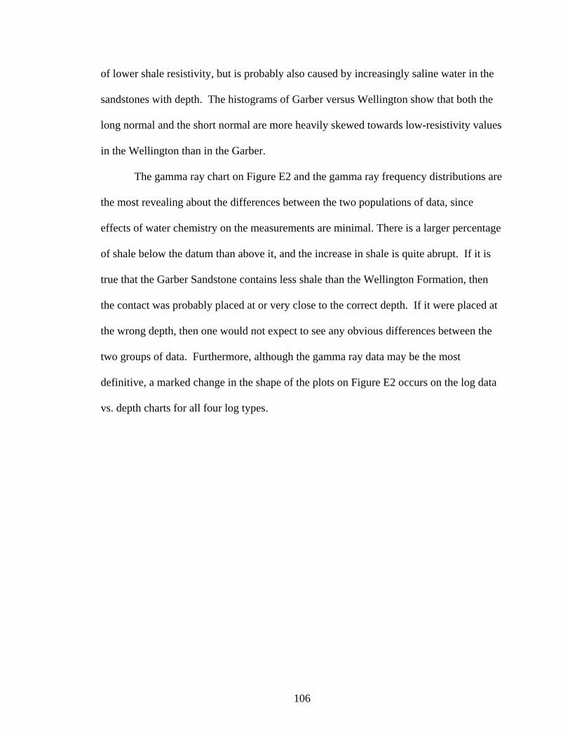
106

of lower shale resistivity, but is probably also caused by increasingly saline water in the

sandstones with depth. The histograms of Garber versus Wellington show that both the

long normal and the short normal are more heavily skewed towards low-resistivity values

in the Wellington than in the Garber.

The gamma ray chart on Figure E2 and the gamma ray frequency distributions are

the most revealing about the differences between the two populations of data, since

effects of water chemistry on the measurements are minimal. There is a larger percentage

of shale below the datum than above it, and the increase in shale is quite abrupt. If it is

true that the Garber Sandstone contains less shale than the Wellington Formation, then

the contact was probably placed at or very close to the correct depth. If it were placed at

the wrong depth, then one would not expect to see any obvious differences between the

two groups of data. Furthermore, although the gamma ray data may be the most

definitive, a marked change in the shape of the plots on Figure E2 occurs on the log data

vs. depth charts for all four log types.

Top of Wellington

Top of Garber

Figure E1. City of Moore Test Well #11, showing lower shale resistivity in the Wellington Formation

107

408NW354W10N1190-97.596235.30154Test Well #1193

708287SE NE173W10N1223-97.532235.34336City of Mustang Test #9B188

649230NW NW SW163W10N1208-97.528835.34057City of Mustang Well #10187

744311SW NE263W9N1155-97.483335.22746Westport Golf Club Test #1185

737298233W9N1164-97.493135.24102City of Norman Well #7-A183

SE NE352W9N1130-97.372835.21274Washington School Test Well #2177

535163NW NW NW172W9N1160-97.440235.26088City of Norman Test Well #1169

537156SE NE NE172W9N1180-97.424735.25908City of Norman Test Well #2168

46148SE SE NE NE162W9N1160-97.407235.25901City of Norman Test Well #3166

53198NW NW NW NE162W9N1183-97.413835.26082City of Norman Test Well #5165

419SW SW SE102W9N1150-97.396135.26274City of Norman Test #10160

403NE NE SE102W9N1160-97.389435.26816City of Norman Test #11159

378NW NW NW NW102W9N1084-97.404935.27538City of Norman Test #6158

400SE SE NE102W9N1145-97.389435.26996City of Norman Test #12157

329NW NE NE102W9N1081-97.391735.27538City of Norman Test #7155

410SE SE SE NE92W9N1113-97.407135.26996City of Norman Test #4153

348NW NW NE92W9N1093-97.413735.27538City of Norman Test #9152

573SE SW84W10N1277-97.646835.3501McBride #189

708289NW NW NE183W10N1205-97.555435.34773City of Mustang #1381

659270NE SE NE173W10N1222-97.531135.34425City of Mustang #979

694228SE SE SE SW163W10N1217-97.521635.33479City of Mustang #1178

682276SE SE SE NE63W10N1271-97.548335.37076City of Mustang Test Well #772

52968SW SE SE13W10N1275-97.462535.36406City of Moore #1 Test Hole71

47678SE SE SW182W10N1198-97.451335.33507City of Moore #2 Test Hole63

49982C NW NE182W10N1245-97.44835.34682City of Moore #3662

331NWNENE182W9N1081-97.391835.27577NormanWW#3727

380NWNWNW102W9N1084-97.405335.27575NormanWW#3626

456NWNWNE142W9N1173-97.378535.26084City of Norman Test #139

Top Well

Top GarbSpot CallSectionRange

Township

DatumSurf LonSurf LatWell NameUWI

408NW354W10N1190-97.596235.30154Test Well #1193

708287SE NE173W10N1223-97.532235.34336City of Mustang Test #9B188

649230NW NW SW163W10N1208-97.528835.34057City of Mustang Well #10187

744311SW NE263W9N1155-97.483335.22746Westport Golf Club Test #1185

737298233W9N1164-97.493135.24102City of Norman Well #7-A183

SE NE352W9N1130-97.372835.21274Washington School Test Well #2177

535163NW NW NW172W9N1160-97.440235.26088City of Norman Test Well #1169

537156SE NE NE172W9N1180-97.424735.25908City of Norman Test Well #2168

46148SE SE NE NE162W9N1160-97.407235.25901City of Norman Test Well #3166

53198NW NW NW NE162W9N1183-97.413835.26082City of Norman Test Well #5165

419SW SW SE102W9N1150-97.396135.26274City of Norman Test #10160

403NE NE SE102W9N1160-97.389435.26816City of Norman Test #11159

378NW NW NW NW102W9N1084-97.404935.27538City of Norman Test #6158

400SE SE NE102W9N1145-97.389435.26996City of Norman Test #12157

329NW NE NE102W9N1081-97.391735.27538City of Norman Test #7155

410SE SE SE NE92W9N1113-97.407135.26996City of Norman Test #4153

348NW NW NE92W9N1093-97.413735.27538City of Norman Test #9152

573SE SW84W10N1277-97.646835.3501McBride #189

708289NW NW NE183W10N1205-97.555435.34773City of Mustang #1381

659270NE SE NE173W10N1222-97.531135.34425City of Mustang #979

694228SE SE SE SW163W10N1217-97.521635.33479City of Mustang #1178

682276SE SE SE NE63W10N1271-97.548335.37076City of Mustang Test Well #772

52968SW SE SE13W10N1275-97.462535.36406City of Moore #1 Test Hole71

47678SE SE SW182W10N1198-97.451335.33507City of Moore #2 Test Hole63

49982C NW NE182W10N1245-97.44835.34682City of Moore #3662

331NWNENE182W9N1081-97.391835.27577NormanWW#3727

380NWNWNW102W9N1084-97.405335.27575NormanWW#3626

456NWNWNE142W9N1173-97.378535.26084City of Norman Test #139

Top Well

Top GarbSpot CallSectionRange

Township

DatumSurf LonSurf LatWell NameUWI

Table E

1. List of wells used in A

ppendix E

108

Figure E2. C

ross plots of digital log data vs. depth. Zero on the y-axis is the proposed contact depth.

109

Ga

rb

er

Mean=81.5

SD=23.14

Ga

rb

er

Mean=-2.08

SD=17.98

We

ll

in

gt

on

Mean=93.43

SD=27.94

We

ll

in

gt

on

Mean=-6.45

SD=15.77

Figure E3. Frequency distribution com

parisons for Garber (top) and

Wellington (bottom

), gamm

a ray data (left) and SP data (right)

110

Ga

rb

er

Mean=34.93

SD=22.1

Ga

rb

er

Mean=42.6

SD=30.93W

el

li

ng

to

n

Mean=28.8

SD=19.23

We

ll

in

gt

on

Mean=30.9

SD=23.38

Figure E4. Frequency distribution com

parisons for Garber (top) and

Wellington (bottom

), long normal data (left) and short norm

al data (right)

111

VITA

Ben Nicholas Abbott

Candidate for the Degree of

Master of Science

Thesis: SUBSURFACE GEOLOGY OF ARSENIC-BEARING PERMIAN SEDIMENTARY ROCKS IN THE GARBER-WELLINGTON INTERVAL OF THE CENTRAL OKLAHOMA AQUIFER, CLEVELAND COUNTY, OKLAHOMA

Major Field: Geology Biographical: Personal Data: Born in Pierce County, Washington in 1978. Raised by wolves.

Education: Graduated from Booker T. Washington High School in Tulsa, Oklahoma, class of 1996. After three years at Tulsa Community College, came to Oklahoma State and graduated in 2002 with a B.S. in Geology. Completed the requirements for the Master of Science degree at Oklahoma State University in December, 2005.

Professional Memberships: Tulsa Geological Society, American Association of

Petroleum Geologists

Name: Ben N. Abbott Date of Degree: December 2005 Institution: Oklahoma State University Location: Stillwater, OK Title of Study: SUBSURFACE GEOLOGY OF ARSENIC-BEARING PERMIAN

SEDIMENTARY ROCKS IN THE GARBER-WELLINGTON INTERVAL OF THE CENTRAL OKLAHOMA AQUIFER, CLEVELAND COUNTY, OKLAHOMA

Pages in Study: 111 Candidate for the Degree of Master of Science The Central Oklahoma Aquifer is an important source of drinking water in central Oklahoma. The major formations making up the aquifer, the Garber Sandstone and the Wellington Formation, consist of fluvial sandstones interbedded with mudstones, siltstones, and conglomerates. Water from some wells has naturally occurring arsenic levels that exceed federal standards. Past work suggests that the arsenic is concentrated in water produced from sandstones isolated by finer-grained rocks. One strategy for remediation is to selectively produce water from low-arsenic zones and to limit water production from sandstones isolated by finer-grained lithofacies. This requires the development of a stratigraphic framework that defines the lateral and vertical distribution of arsenic-prone lithofacies. Mapping of lithofacies suggests that arsenic concentration is most closely associated with shaly sandstone distribution; based on the maps, there are two favorable areas for new water wells, and at least one area that should be avoided. Advisor’s Approval: Stanley T. Paxton