Embed Size (px)
Citation preview
Substring Statistics
Kyoji Umemura
Kenneth Church
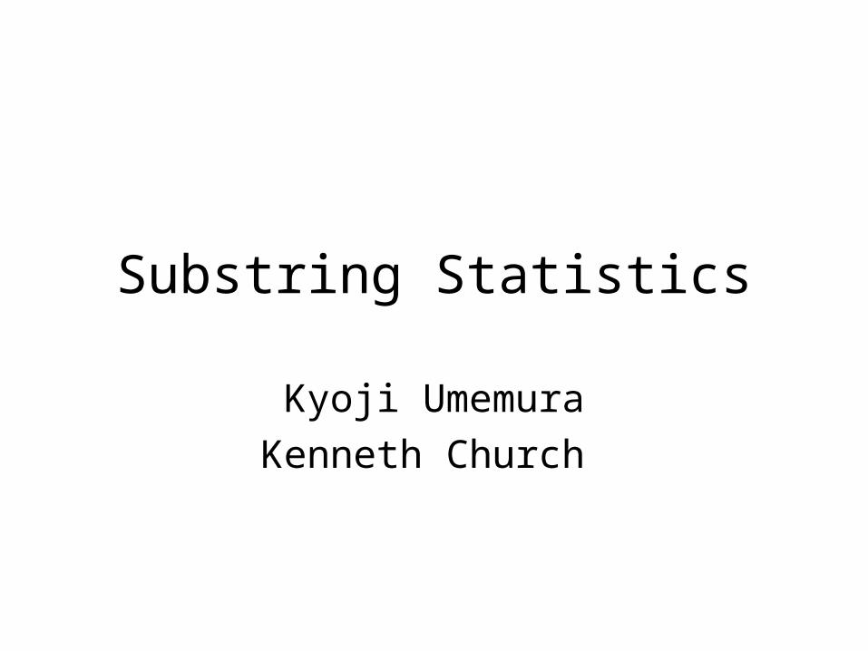
Goal: Words Substrings(Anything you can do with words, we can do with substrings)
• Haven’t achieved this goal– But we can do more with substrings than you might have thought
• Review: – Using Suffix Arrays to compute Term Frequency and Document
Frequency for All Substrings in a Corpus (Yamamoto & Church)– Tri-grams Million-grams
• Tutorial: Make substring statistics look easy– Previous treatments are (a bit) inaccessible
• Generalization: – Document Frequency (df) dfk (adaptation)
• Applications– Word Breaking (Japanese & Chinese)– Term Extraction for Information Retrieval
Sound Bite
Sound Bite
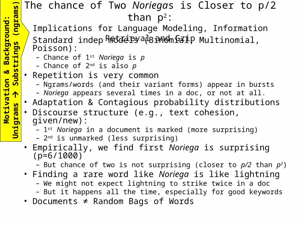
The chance of Two Noriegas is Closer to p/2 than p2:Implications for Language Modeling, Information Retrieval and Gzip
• Standard indep models (Binomial, Multinomial, Poisson):– Chance of 1st Noriega is p– Chance of 2nd is also p
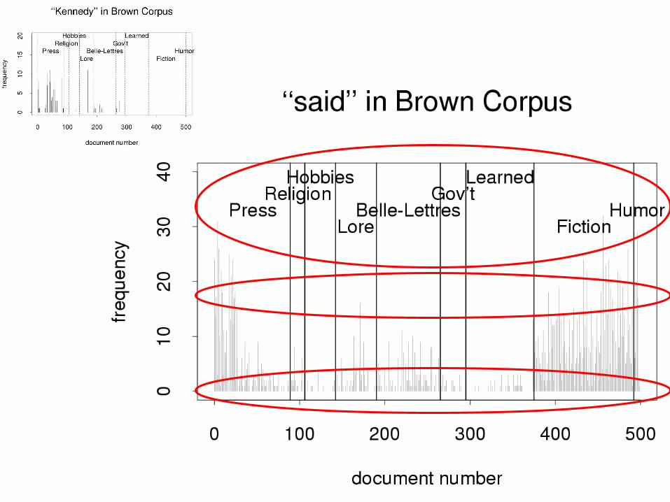
• Repetition is very common– Ngrams/words (and their variant forms) appear in bursts– Noriega appears several times in a doc, or not at all.
• Adaptation & Contagious probability distributions• Discourse structure (e.g., text cohesion, given/new):
– 1st Noriega in a document is marked (more surprising)– 2nd is unmarked (less surprising)
• Empirically, we find first Noriega is surprising (p≈6/1000)– But chance of two is not surprising (closer to p/2 than p2)
• Finding a rare word like Noriega is like lightning– We might not expect lightning to strike twice in a doc– But it happens all the time, especially for good keywords
• Documents ≠ Random Bags of Words
Mo
tiva
tio
n &
Bac
kgro
un
d:
Un
igra
ms
S
ub
stri
ng
s (n
gra
ms)
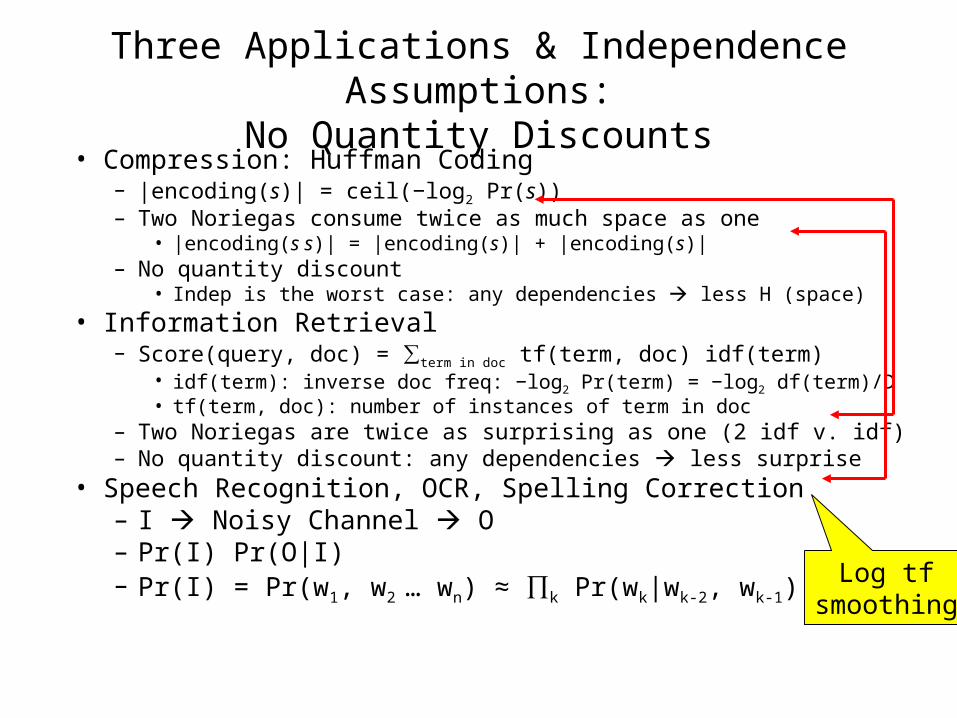
Three Applications & Independence Assumptions:No Quantity Discounts
• Compression: Huffman Coding– |encoding(s)| = ceil(−log2 Pr(s))– Two Noriegas consume twice as much space as one
• |encoding(s s)| = |encoding(s)| + |encoding(s)|– No quantity discount
• Indep is the worst case: any dependencies less H (space)
• Information Retrieval– Score(query, doc) = ∑term in doc tf(term, doc) idf(term)
• idf(term): inverse doc freq: −log2 Pr(term) = −log2 df(term)/D• tf(term, doc): number of instances of term in doc
– Two Noriegas are twice as surprising as one (2 idf v. idf)– No quantity discount: any dependencies less surprise
• Speech Recognition, OCR, Spelling Correction– I Noisy Channel O– Pr(I) Pr(O|I)– Pr(I) = Pr(w1, w2 … wn) ≈ ∏k Pr(wk|wk-2, wk-1)
Log tfsmoothing
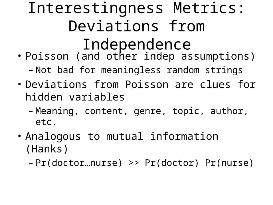
Interestingness Metrics:Deviations from Independence
• Poisson (and other indep assumptions)– Not bad for meaningless random strings
• Deviations from Poisson are clues for hidden variables– Meaning, content, genre, topic, author, etc.
• Analogous to mutual information (Hanks)– Pr(doctor…nurse) >> Pr(doctor) Pr(nurse)
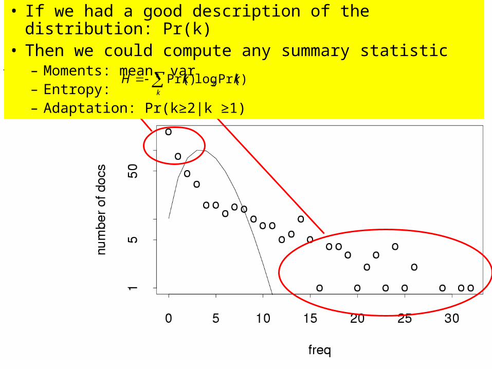
• If we had a good description of the distribution: Pr(k)• Then we could compute any summary statistic
– Moments: mean, var– Entropy: – Adaptation: Pr(k≥2|k ≥1)
k
kkH )Pr(log)Pr( 2
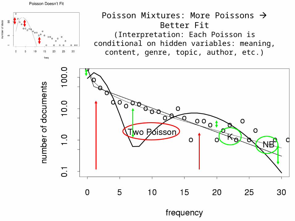
Poisson Mixtures: More Poissons Better Fit(Interpretation: Each Poisson is conditional on hidden variables: meaning, content, genre, topic, author, etc.)
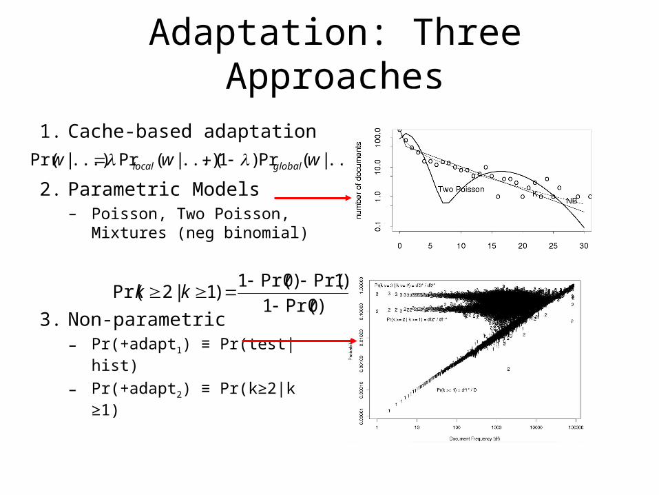
1. Cache-based adaptation
2. Parametric Models– Poisson, Two Poisson,
Mixtures (neg binomial)
3. Non-parametric– Pr(+adapt1) ≡ Pr(test|hist)
– Pr(+adapt2) ≡ Pr(k≥2|k ≥1)
Adaptation: Three Approaches
)0Pr(1
)1Pr()0Pr(1)1|2Pr(
kk
...)|(Pr)1(...)|(Pr...)|Pr( www globallocal
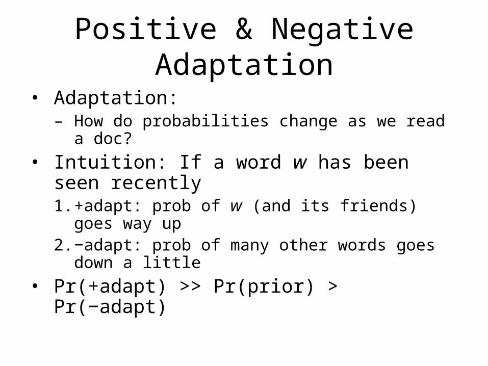
Positive & Negative Adaptation
• Adaptation:– How do probabilities change as we read a doc?
• Intuition: If a word w has been seen recently1. +adapt: prob of w (and its friends) goes way up2. −adapt: prob of many other words goes down a little
• Pr(+adapt) >> Pr(prior) > Pr(−adapt)
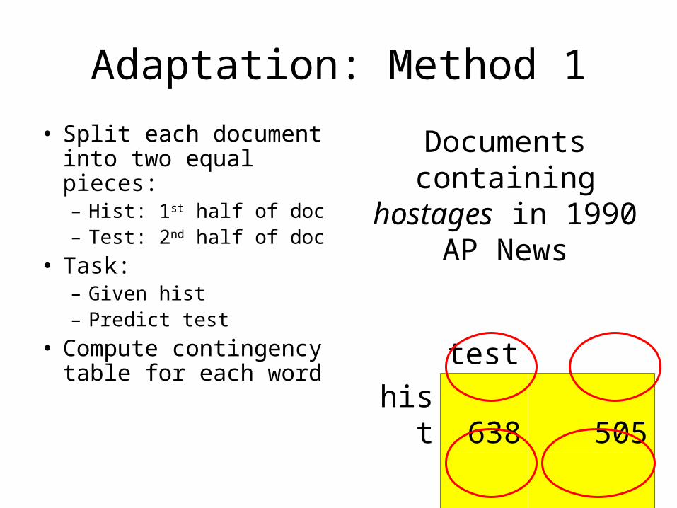
Adaptation: Method 1
• Split each document into two equal pieces:– Hist: 1st half of doc– Test: 2nd half of doc
• Task: – Given hist– Predict test
• Compute contingency table for each word
Documents containing hostages
in 1990 AP News
test
hist 638 505
557 76,787
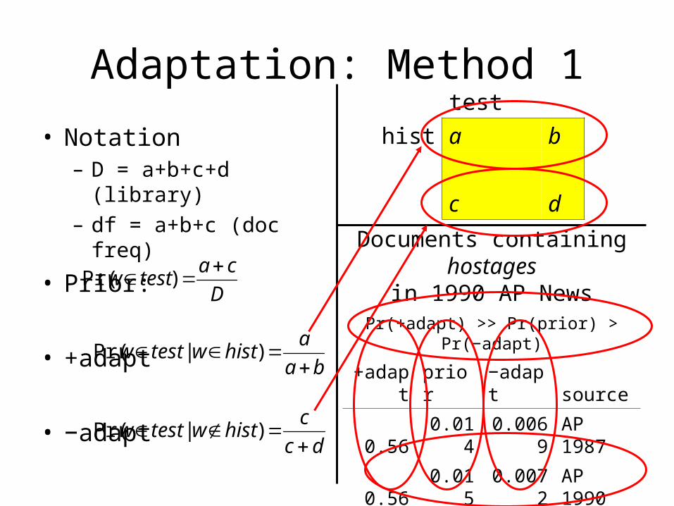
Adaptation: Method 1
• Notation– D = a+b+c+d (library)– df = a+b+c (doc freq)
• Prior:
• +adapt
• −adapt
test
hist a b
c d
Documents containing hostages
in 1990 AP NewsPr(+adapt) >> Pr(prior) > Pr(−adapt)
+adapt prior −adapt source
0.56 0.014 0.0069 AP 1987
0.56 0.015 0.0072 AP 1990
0.59 0.013 0.0057 AP 1991
0.39 0.004 0.0030 AP 1993
D
catestw
)Pr(
ba
ahistwtestw
)|Pr(
dc
chistwtestw
)|Pr(
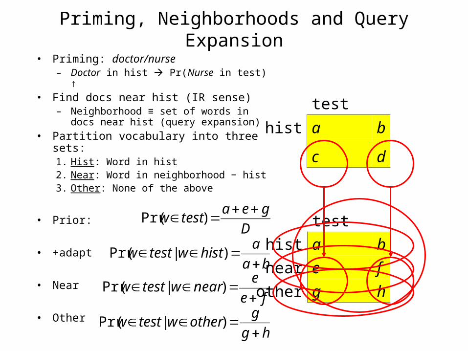
Priming, Neighborhoods and Query Expansion
• Priming: doctor/nurse– Doctor in hist Pr(Nurse in test) ↑
• Find docs near hist (IR sense)– Neighborhood ≡ set of words in docs
near hist (query expansion)
• Partition vocabulary into three sets:1. Hist: Word in hist2. Near: Word in neighborhood − hist3. Other: None of the above
• Prior:
• +adapt
• Near
• Other
test
hist a b
c d
test
hist a b
near e f
other g h
D
geatestw
)Pr(
ba
ahistwtestw
)|Pr(
fe
enearwtestw
)|Pr(
hg
gotherwtestw
)|Pr(
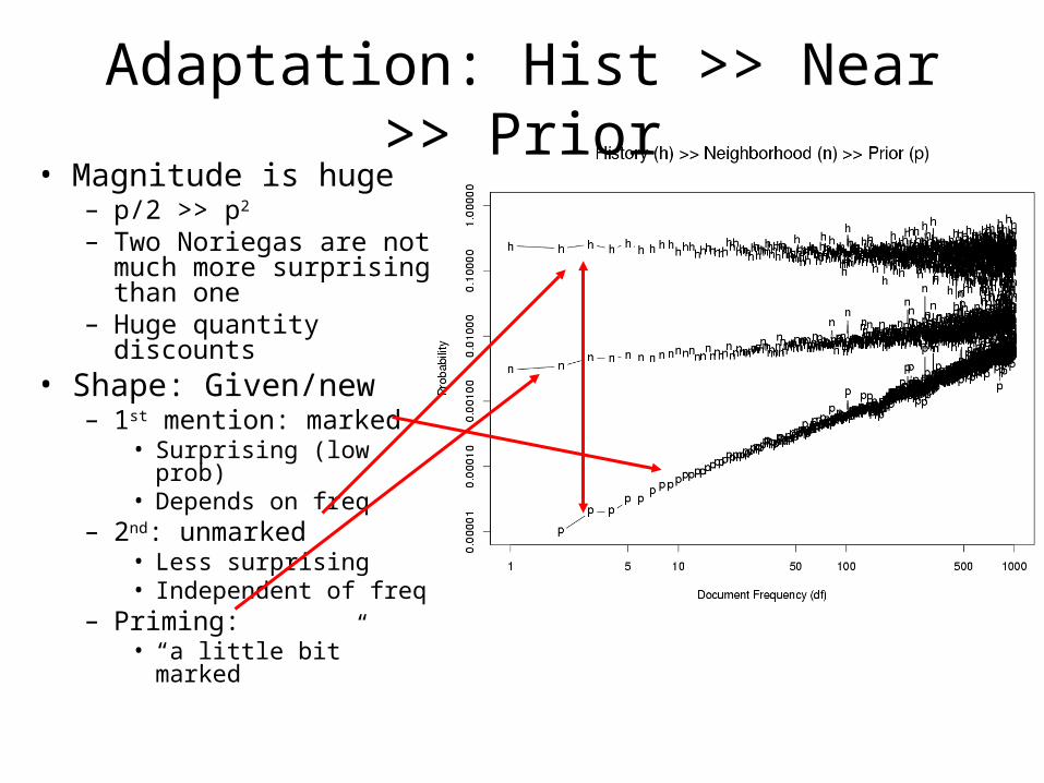
Adaptation: Hist >> Near >> Prior• Magnitude is huge
– p/2 >> p2
– Two Noriegas are not much more surprising than one
– Huge quantity discounts• Shape: Given/new
– 1st mention: marked• Surprising (low prob)• Depends on freq
– 2nd: unmarked• Less surprising• Independent of freq
– Priming: • “a little bit” marked
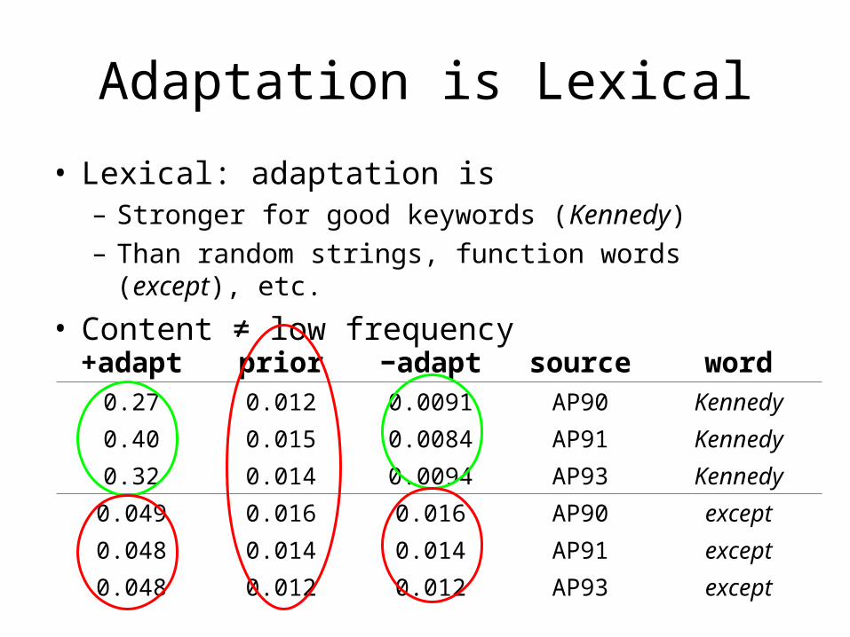
Adaptation is Lexical
• Lexical: adaptation is– Stronger for good keywords (Kennedy)– Than random strings, function words (except), etc.
• Content ≠ low frequency
+adapt prior −adapt source word0.27 0.012 0.0091 AP90 Kennedy
0.40 0.015 0.0084 AP91 Kennedy
0.32 0.014 0.0094 AP93 Kennedy
0.049 0.016 0.016 AP90 except
0.048 0.014 0.014 AP91 except
0.048 0.012 0.012 AP93 except
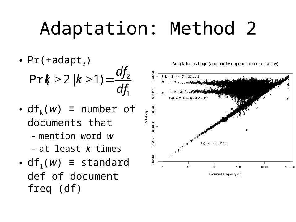
Adaptation: Method 2
• Pr(+adapt2)
• dfk(w) ≡ number of documents that– mention word w– at least k times
• df1(w) ≡ standard def of document freq (df)
1
2)1|2Pr(df
dfkk
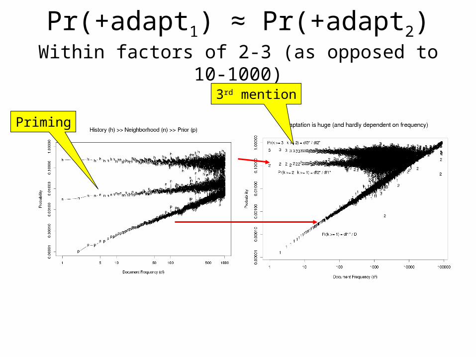
Pr(+adapt1) ≈ Pr(+adapt2)Within factors of 2-3 (as opposed to 10-1000)
3rd mention
Priming
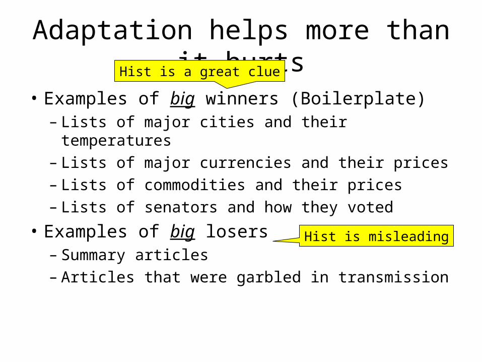
Adaptation helps more than it hurts
• Examples of big winners (Boilerplate)– Lists of major cities and their temperatures– Lists of major currencies and their prices– Lists of commodities and their prices– Lists of senators and how they voted
• Examples of big losers– Summary articles– Articles that were garbled in transmission
Hist is a great clue
Hist is misleading
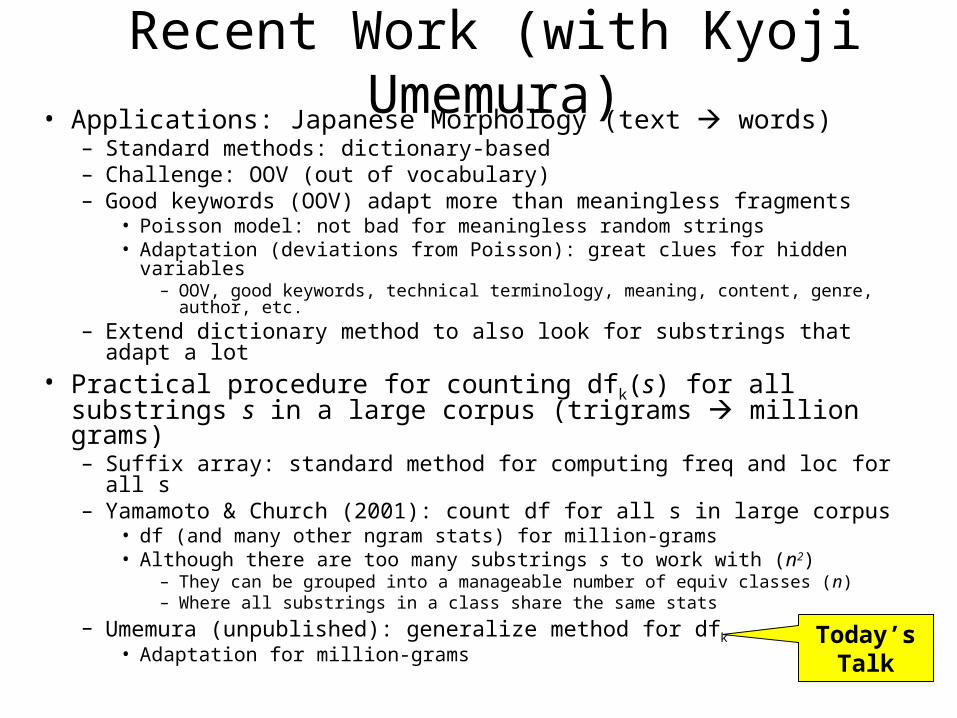
Recent Work (with Kyoji Umemura)• Applications: Japanese Morphology (text words)
– Standard methods: dictionary-based– Challenge: OOV (out of vocabulary)– Good keywords (OOV) adapt more than meaningless fragments
• Poisson model: not bad for meaningless random strings• Adaptation (deviations from Poisson): great clues for hidden variables
– OOV, good keywords, technical terminology, meaning, content, genre, author, etc.
– Extend dictionary method to also look for substrings that adapt a lot
• Practical procedure for counting dfk(s) for all substrings s in a large corpus (trigrams million grams)– Suffix array: standard method for computing freq and loc for all s– Yamamoto & Church (2001): count df for all s in large corpus
• df (and many other ngram stats) for million-grams• Although there are too many substrings s to work with (n2)
– They can be grouped into a manageable number of equiv classes (n)– Where all substrings in a class share the same stats
– Umemura (unpublished): generalize method for dfk
• Adaptation for million-grams
Today’s Talk
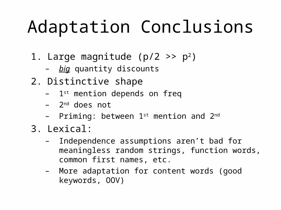
Adaptation Conclusions
1. Large magnitude (p/2 >> p2)– big quantity discounts
2. Distinctive shape– 1st mention depends on freq– 2nd does not– Priming: between 1st mention and 2nd
3. Lexical: – Independence assumptions aren’t bad for meaningless
random strings, function words, common first names, etc.– More adaptation for content words (good keywords, OOV)
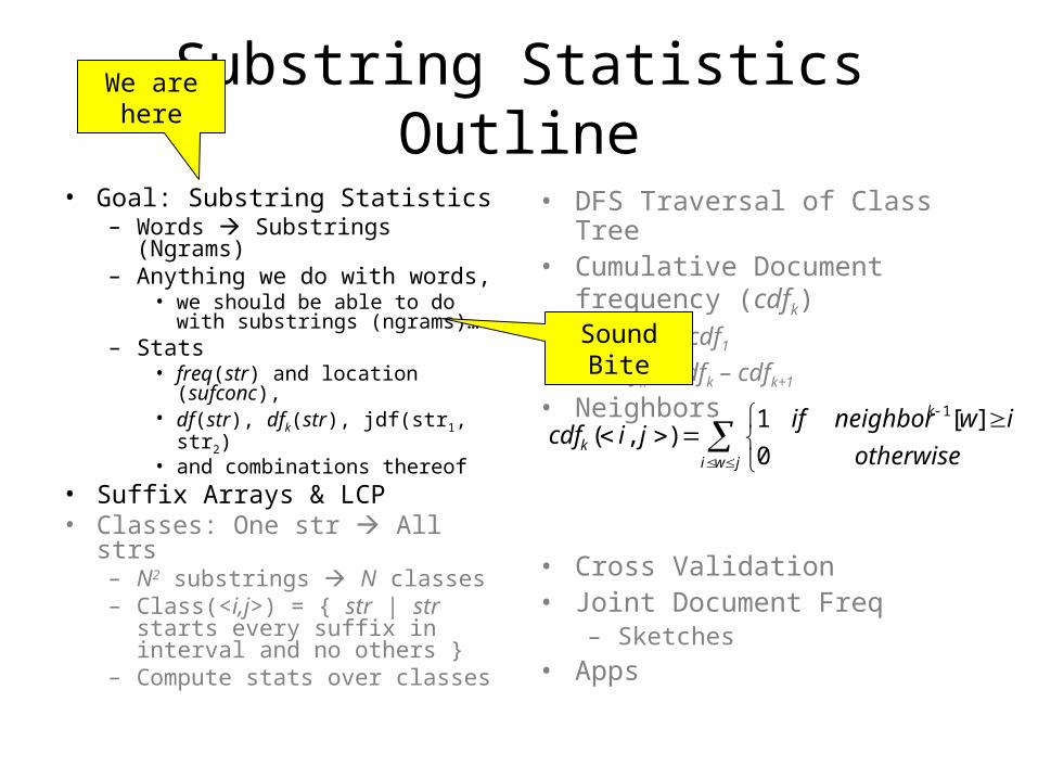
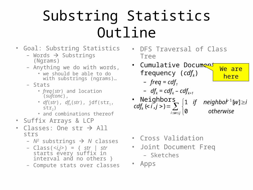
Substring StatisticsOutline
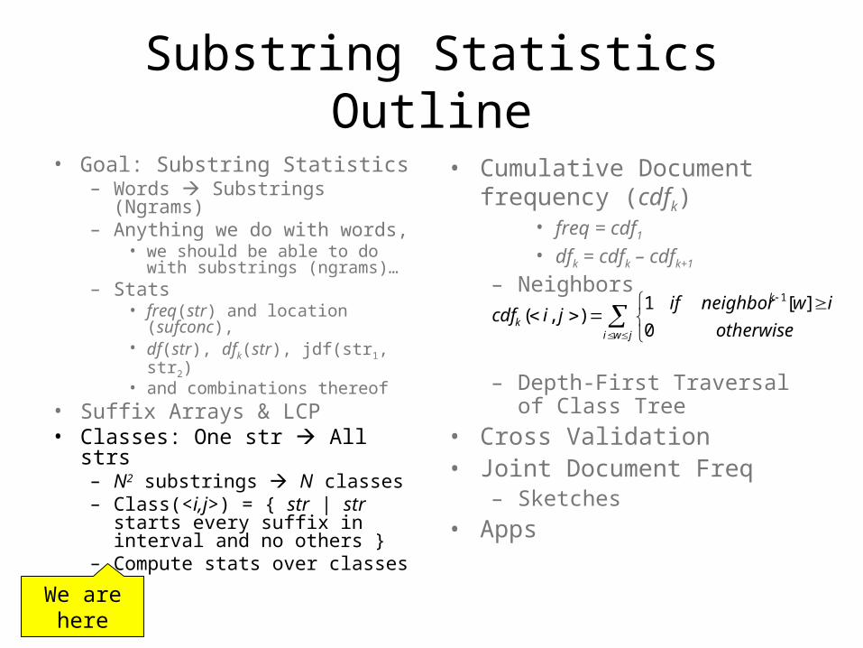
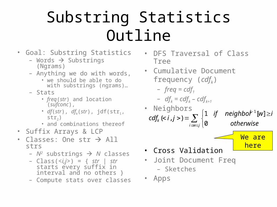
• Goal: Substring Statistics– Words Substrings (Ngrams)– Anything we do with words,
• we should be able to do with substrings (ngrams)…
– Stats• freq(str) and location
(sufconc), • df(str), dfk(str), jdf(str1, str2)• and combinations thereof
• Suffix Arrays & LCP• Classes: One str All strs
– N2 substrings N classes– Class(<i,j>) = { str | str starts
every suffix in interval and no others }
– Compute stats over classes
• DFS Traversal of Class Tree• Cumulative Document
frequency (cdfk)– freq = cdf1
– dfk = cdfk – cdfk+1
• Neighbors
• Cross Validation• Joint Document Freq
– Sketches
• Apps
jwi
k
kotherwise
iwneighborifjicdf
0
][1),(
1
We are here
Sound Bite
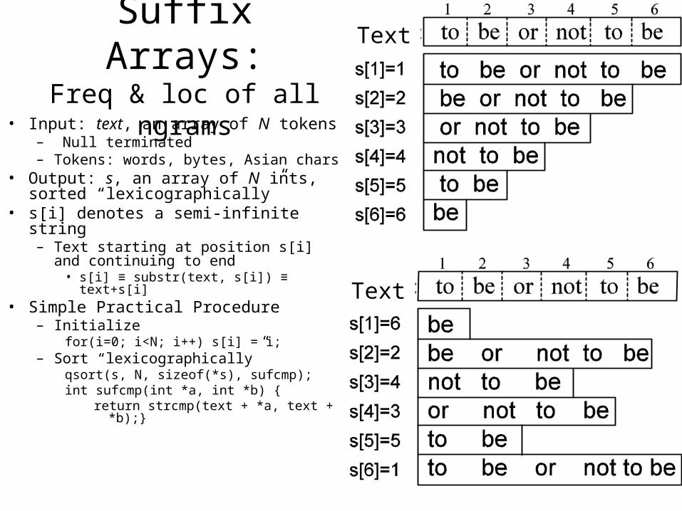
Suffix Arrays:Freq & loc of all ngrams
• Input: text, an array of N tokens– Null terminated– Tokens: words, bytes, Asian chars
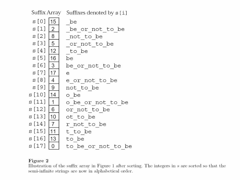
• Output: s, an array of N ints, sorted “lexicographically”
• s[i] denotes a semi-infinite string– Text starting at position s[i] and
continuing to end• s[i] ≡ substr(text, s[i]) ≡ text+s[i]
• Simple Practical Procedure– Initialize
for(i=0; i<N; i++) s[i] = i;– Sort “lexicographically”
qsort(s, N, sizeof(*s), sufcmp);int sufcmp(int *a, int *b) {
return strcmp(text + *a, text + *b);}
Text
Text
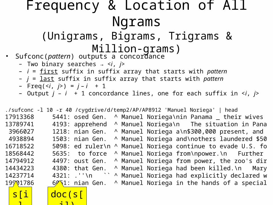
Frequency & Location of All Ngrams(Unigrams, Bigrams, Trigrams & Million-grams)
• Sufconc(pattern) outputs a concordance– Two binary searches → <i, j>– i = first suffix in suffix array that starts with pattern– j = last suffix in suffix array that starts with pattern– Freq(<i, j>) = j – i + 1– Output j – i + 1 concordance lines, one for each suffix in <i, j>
./sufconc -l 10 -r 40 /cygdrive/d/temp2/AP/AP8912 'Manuel Noriega' | head17913368 5441: osed Gen. ^ Manuel Noriega\nin Panama _ their wives 13789741 4193: apprehend ^ Manuel Noriega\n The situation in Pana 3966027 1218: nian Gen. ^ Manuel Noriega a\n$300,000 present, and 4938894 1503: nian Gen. ^ Manuel Noriega and\nothers laundered $5016718522 5098: ed ruler\n ^ Manuel Noriega continue to evade U.S. fo18568442 5635: to force ^ Manuel Noriega from\npower.\n Further 14794912 4497: oust Gen. ^ Manuel Noriega from power, the zoo's dir14434223 4380: that Gen. ^ Manuel Noriega had been killed.\n Mary14237714 4321: .''\n `` ^ Manuel Noriega had explicitly declared w19901786 6061: nian Gen. ^ Manuel Noriega in the hands of a special
s[i] doc(s[i])
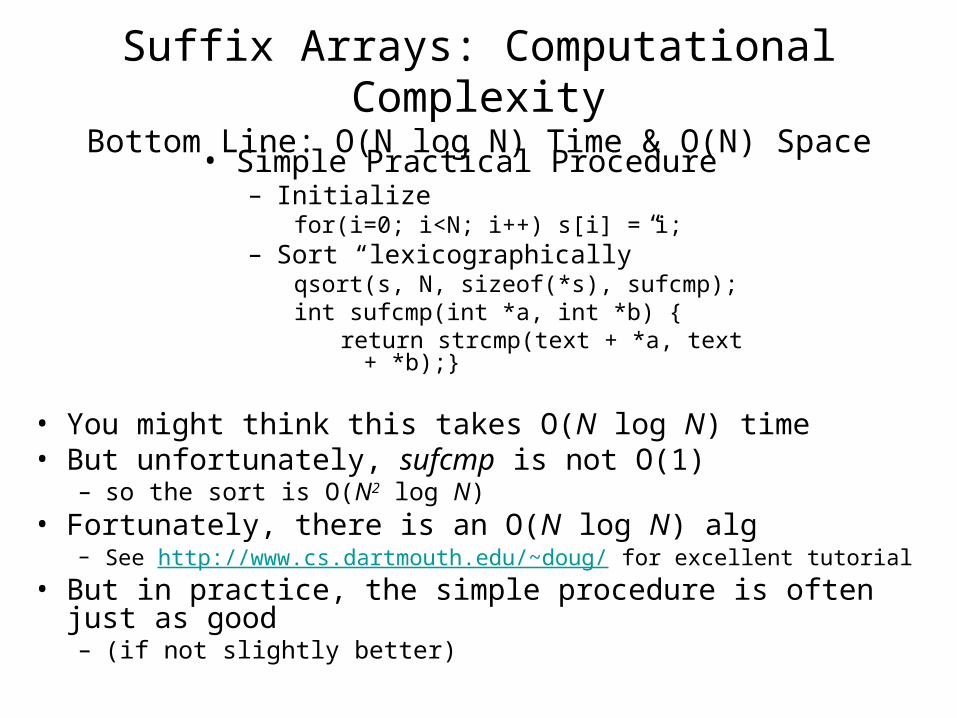
Suffix Arrays: Computational ComplexityBottom Line: O(N log N) Time & O(N) Space
• You might think this takes O(N log N) time• But unfortunately, sufcmp is not O(1)
– so the sort is O(N2 log N)• Fortunately, there is an O(N log N) alg
– See http://www.cs.dartmouth.edu/~doug/ for excellent tutorial
• But in practice, the simple procedure is often just as good– (if not slightly better)
• Simple Practical Procedure– Initialize
for(i=0; i<N; i++) s[i] = i;– Sort “lexicographically”
qsort(s, N, sizeof(*s), sufcmp);int sufcmp(int *a, int *b) {
return strcmp(text + *a, text + *b);}
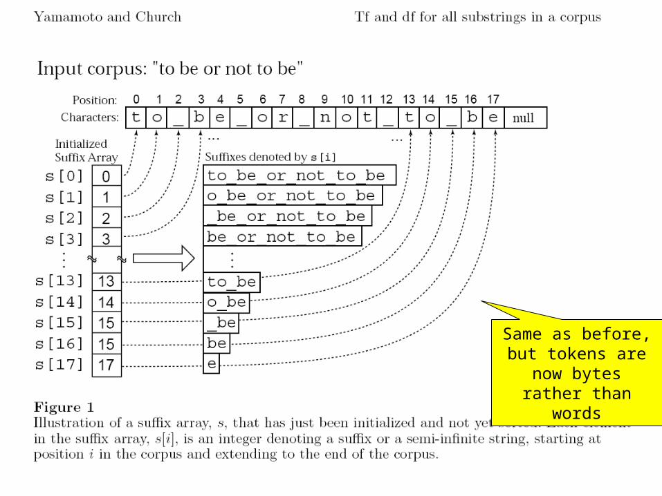
Same as before, but tokens are now bytes
rather than words
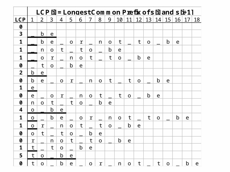
LCP 1 2 3 4 5 6 7 8 9 10 11 12 13 14 15 16 17 1803 _ b e
1 _ b e _ o r _ n o t _ t o _ b e
1 _ n o t _ t o _ b e
1 _ o r _ n o t _ t o _ b e
0 _ t o _ b e2 b e
0 b e _ o r _ n o t _ t o _ b e1 e
0 e _ o r _ n o t _ t o _ b e0 n o t _ t o _ b e4 o _ b e
1 o _ b e _ o r _ n o t _ t o _ b e
1 o r _ n o t _ t o _ b e
0 o t _ t o _ b e0 r _ n o t _ t o _ b e1 t _ t o _ b e
5 t o _ b e
0 t o _ b e _ o r _ n o t _ t o _ b e
LCP[i] = Longest Common Prefix of s[i] and s[i+1]
Dis
trib
utio
n of
LC
Ps
(198
9 A
P N
ews)
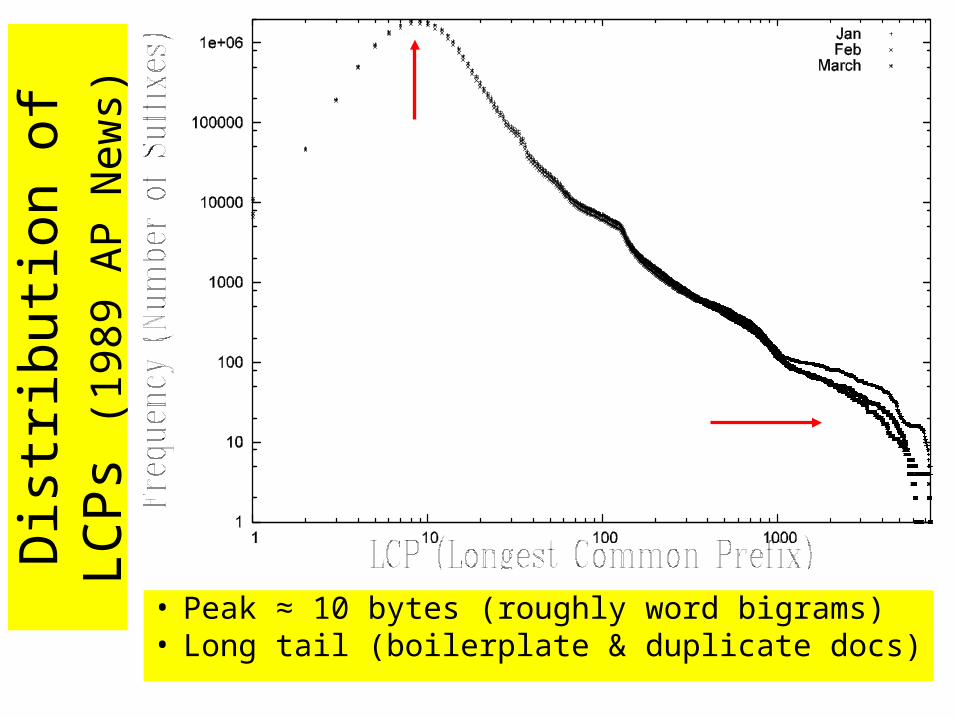
• Peak ≈ 10 bytes (roughly word bigrams)• Long tail (boilerplate & duplicate docs)
Substring StatisticsOutline
• Goal: Substring Statistics– Words Substrings (Ngrams)– Anything we do with words,
• we should be able to do with substrings (ngrams)…
– Stats• freq(str) and location
(sufconc), • df(str), dfk(str), jdf(str1, str2)• and combinations thereof
• Suffix Arrays & LCP• Classes: One str All strs
– N2 substrings N classes– Class(<i,j>) = { str | str starts
every suffix in interval and no others }
– Compute stats over classes
• Cumulative Document frequency (cdfk)
• freq = cdf1
• dfk = cdfk – cdfk+1
– Neighbors
– Depth-First Traversal of Class Tree
• Cross Validation• Joint Document Freq
– Sketches
• Apps
jwi
k
kotherwise
iwneighborifjicdf
0
][1),(
1
We are here
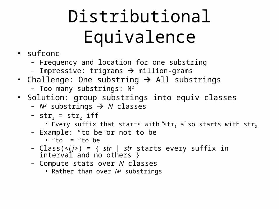
Distributional Equivalence• sufconc
– Frequency and location for one substring– Impressive: trigrams million-grams
• Challenge: One substring All substrings– Too many substrings: N2
• Solution: group substrings into equiv classes– N2 substrings N classes– str1 = str2 iff
• Every suffix that starts with str1 also starts with str2
– Example: “to be or not to be”• “to” = “to be”
– Class(<i,j>) = { str | str starts every suffix in interval and no others }– Compute stats over N classes
• Rather than over N2 substrings
Grouping Substrings into Classess LCP 1 2 3 4 5 6 7 8 9 10 11 12 13 14 15 16 17 180 01 3 _ b e
2 1 _ b e _ o r _ n o t _ t o _ b e
3 1 _ n o t _ t o _ b e
4 1 _ o r _ n o t _ t o _ b e
5 0 _ t o _ b e6 2 b e
7 0 b e _ o r _ n o t _ t o _ b e8 1 e
9 0 e _ o r _ n o t _ t o _ b e10 0 n o t _ t o _ b e11 4 o _ b e
12 1 o _ b e _ o r _ n o t _ t o _ b e
13 1 o r _ n o t _ t o _ b e
14 0 o t _ t o _ b e15 0 r _ n o t _ t o _ b e16 1 t _ t o _ b e
17 5 t o _ b e
18 0 t o _ b e _ o r _ n o t _ t o _ b e
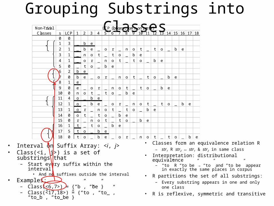
Non-Trivial Classes
LCP (longest common prefix)
• Interval on Suffix Array: <i, j>• Class(<i, j>) is a set of substrings that
– Start every suffix within the interval• And no suffixes outside the interval
• Examples:– Class(<6,7>) = {“b”, “be”}– Class(<17,18>) = {“to”, “to_”, “to_b”,
“to_be”}
• Classes form an equivalence relation R– str1 R str2 ↔ str1 & str2 in same class
• Interpretation: distributional equivalence– “to” R “to be” → “to” and “to be” appear in
exactly the same places in corpus
• R partitions the set of all substrings: – Every substring appears in one and only one
class
• R is reflexive, symmetric and transitive
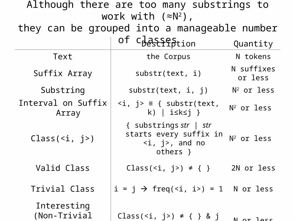
Although there are too many substrings to work with (≈N2),they can be grouped into a manageable number of classes
Description Quantity
Text the Corpus N tokens
Suffix Array substr(text, i)N suffixes
or less
Substring substr(text, i, j) N2 or less
Interval on Suffix Array <i, j> ≡ { substr(text, k) | i≤k≤j } N2 or less
Class(<i, j>){ substrings str | str starts every
suffix in <i, j>, and no others }N2 or less
Valid Class Class(<i, j>) ≠ { } 2N or less
Trivial Class i = j freq(<i, i>) = 1 N or less
Interesting(Non-Trivial Valid)
ClassClass(<i, j>) ≠ { } & j > i N or less
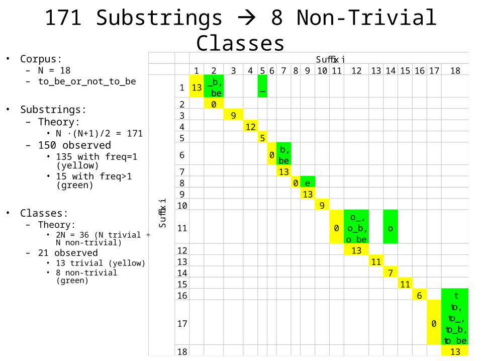
171 Substrings 8 Non-Trivial Classes• Corpus:
– N = 18– to_be_or_not_to_be
• Substrings: – Theory:
• N ∙(N+1)/2 = 171– 150 observed
• 135 with freq=1 (yellow)
• 15 with freq>1 (green)
• Classes: – Theory:
• 2N = 36 (N trivial + N non-trivial)
– 21 observed• 13 trivial (yellow)• 8 non-trivial (green)
1 2 3 4 5 6 7 8 9 10 11 12 13 14 15 16 17 18
1 13_b, _be
_
2 03 94 125 5
6 0b, be
7 138 0 e9 1310 9
11 0o_,
o_b, o_be
o
12 1313 1114 715 1116 6 t
17 0
to, to_,
to_b, to_be
18 13
Su
ffix
i
Suffix j
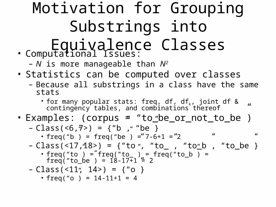
Motivation for Grouping Substrings into Equivalence Classes
• Computational Issues:– N is more manageable than N2
• Statistics can be computed over classes– Because all substrings in a class have the same stats
• for many popular stats: freq, df, dfk, joint df & contingency tables, and combinations thereof
• Examples: (corpus = “to_be_or_not_to_be”)– Class(<6,7>) = {“b”, “be”}
• freq(“b”) = freq(“be”) = 7-6+1 = 2– Class(<17,18>) = {“to”, “to_”, “to_b”, “to_be”}
• freq(“to”) = freq(“to_”) = freq(“to_b”) = freq(“to_be”) = 18-17+1 = 2
– Class(<11, 14>) = {“o”}• freq(“o”) = 14-11+1 = 4
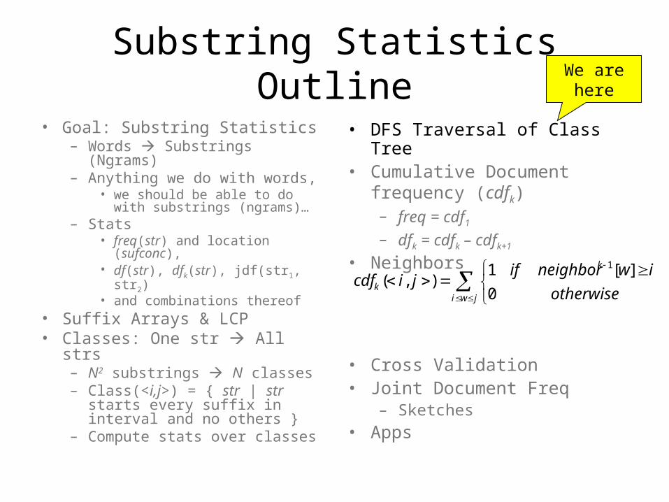
Substring StatisticsOutline
• Goal: Substring Statistics– Words Substrings (Ngrams)– Anything we do with words,
• we should be able to do with substrings (ngrams)…
– Stats• freq(str) and location
(sufconc), • df(str), dfk(str), jdf(str1, str2)• and combinations thereof
• Suffix Arrays & LCP• Classes: One str All strs
– N2 substrings N classes– Class(<i,j>) = { str | str starts
every suffix in interval and no others }
– Compute stats over classes
• DFS Traversal of Class Tree• Cumulative Document
frequency (cdfk)– freq = cdf1
– dfk = cdfk – cdfk+1
• Neighbors
• Cross Validation• Joint Document Freq
– Sketches
• Apps
jwi
k
kotherwise
iwneighborifjicdf
0
][1),(
1
We are here
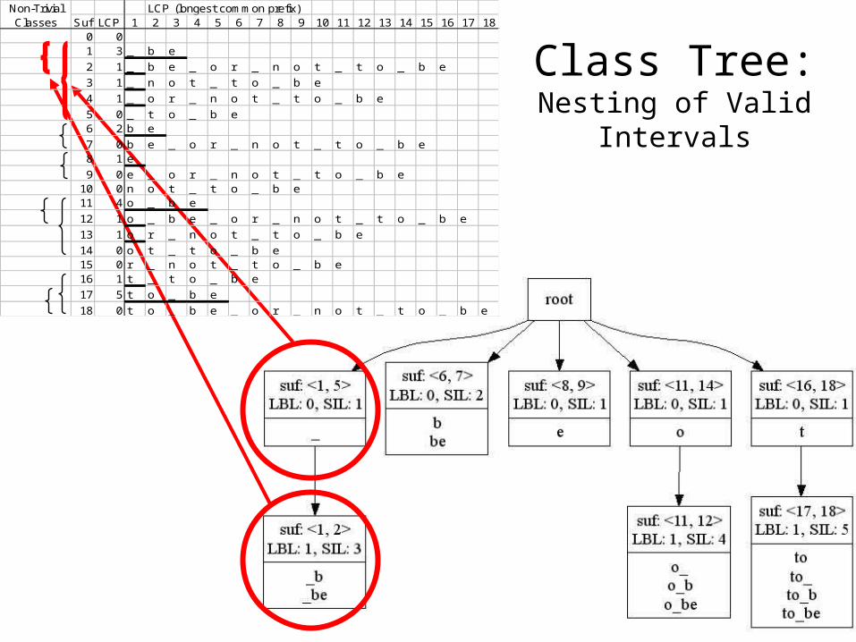
Class Tree:Nesting of Valid Intervals
LCP (longest common prefix)Suf LCP 1 2 3 4 5 6 7 8 9 10 11 12 13 14 15 16 17 18
0 01 3 _ b e
2 1 _ b e _ o r _ n o t _ t o _ b e
3 1 _ n o t _ t o _ b e
4 1 _ o r _ n o t _ t o _ b e
5 0 _ t o _ b e6 2 b e
7 0 b e _ o r _ n o t _ t o _ b e8 1 e
9 0 e _ o r _ n o t _ t o _ b e10 0 n o t _ t o _ b e11 4 o _ b e
12 1 o _ b e _ o r _ n o t _ t o _ b e
13 1 o r _ n o t _ t o _ b e
14 0 o t _ t o _ b e15 0 r _ n o t _ t o _ b e16 1 t _ t o _ b e
17 5 t o _ b e
18 0 t o _ b e _ o r _ n o t _ t o _ b e
Non-Trivial Classes
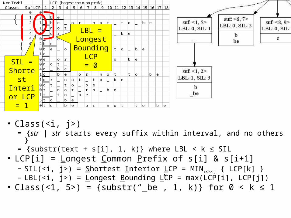
• Class(<i, j>) = {str | str starts every suffix within interval, and no others } = {substr(text + s[i], 1, k)} where LBL < k ≤ SIL
• LCP[i] = Longest Common Prefix of s[i] & s[i+1]– SIL(<i, j>) = Shortest Interior LCP = MINi≤k<j { LCP[k] }– LBL(<i, j>) = Longest Bounding LCP = max(LCP[i], LCP[j])
• Class(<1, 5>) = {substr(“_be”, 1, k)} for 0 < k ≤ 1
LBL = Longest
BoundingLCP= 0SIL =
Shortest Interior
LCP= 1
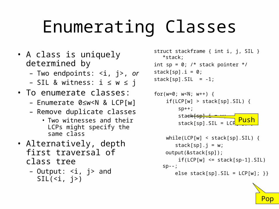
Enumerating Classes
• A class is uniquely determined by– Two endpoints: <i, j>, or– SIL & witness: i ≤ w ≤ j
• To enumerate classes:– Enumerate 0≤w<N & LCP[w]– Remove duplicate classes
• Two witnesses and their LCPs might specify the same class
• Alternatively, depth first traversal of class tree– Output: <i, j> and SIL(<i, j>)
struct stackframe { int i, j, SIL } *stack;
int sp = 0; /* stack pointer */
stack[sp].i = 0;
stack[sp].SIL = -1;
for(w=0; w<N; w++) {
if(LCP[w] > stack[sp].SIL) {
sp++;
stack[sp].i = w;
stack[sp].SIL = LCP[w]; }
while(LCP[w] < stack[sp].SIL) {
stack[sp].j = w;
output(&stack[sp]);
if(LCP[w] <= stack[sp-1].SIL) sp--;
else stack[sp].SIL = LCP[w]; }}
Push
Pop
LCP (longest common prefix)Suf LCP 1 2 3 4 5 6 7 8 9 10 11 12 13 14 15 16 17 18
0 01 3 _ b e
2 1 _ b e _ o r _ n o t _ t o _ b e
3 1 _ n o t _ t o _ b e
4 1 _ o r _ n o t _ t o _ b e
5 0 _ t o _ b e6 2 b e
7 0 b e _ o r _ n o t _ t o _ b e8 1 e
9 0 e _ o r _ n o t _ t o _ b e10 0 n o t _ t o _ b e11 4 o _ b e
12 1 o _ b e _ o r _ n o t _ t o _ b e
13 1 o r _ n o t _ t o _ b e
14 0 o t _ t o _ b e15 0 r _ n o t _ t o _ b e16 1 t _ t o _ b e
17 5 t o _ b e
18 0 t o _ b e _ o r _ n o t _ t o _ b e
Non-Trivial Classes
1
2
3
4
5
6
7
8
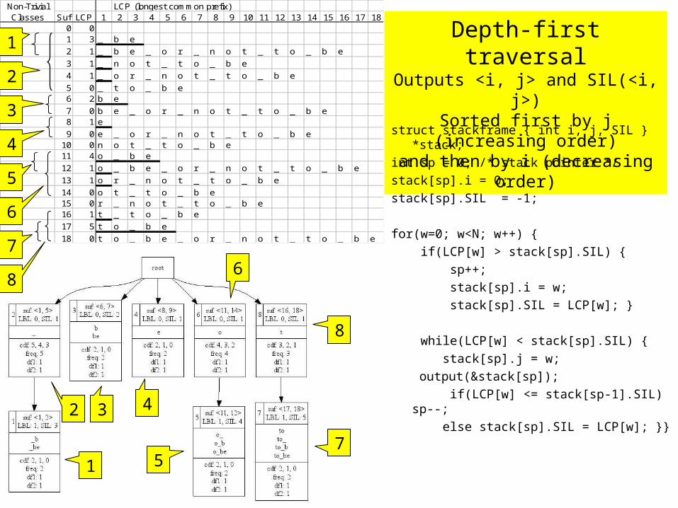
Depth-first traversalOutputs <i, j> and SIL(<i, j>)
Sorted first by j (increasing order)and then by i (decreasing order)
1
32 4
5
6
8
7
struct stackframe { int i, j, SIL } *stack;
int sp = 0; /* stack pointer */
stack[sp].i = 0;
stack[sp].SIL = -1;
for(w=0; w<N; w++) {
if(LCP[w] > stack[sp].SIL) {
sp++;
stack[sp].i = w;
stack[sp].SIL = LCP[w]; }
while(LCP[w] < stack[sp].SIL) {
stack[sp].j = w;
output(&stack[sp]);
if(LCP[w] <= stack[sp-1].SIL) sp--;
else stack[sp].SIL = LCP[w]; }}
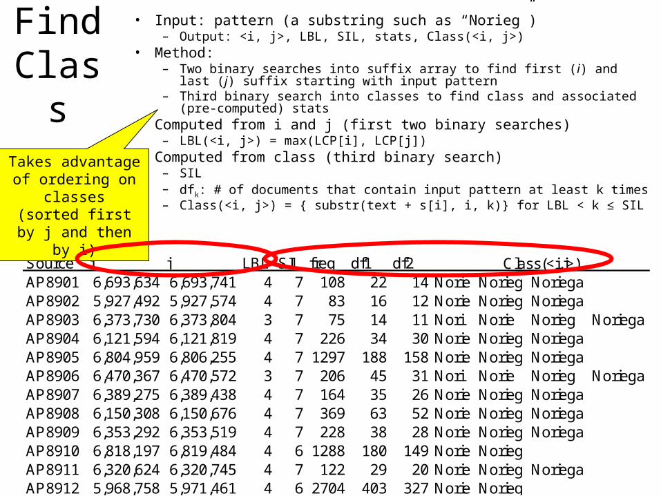
Find Class
• Input: pattern (a substring such as “Norieg”)– Output: <i, j>, LBL, SIL, stats, Class(<i, j>)
• Method: – Two binary searches into suffix array to find first (i) and last (j) suffix
starting with input pattern– Third binary search into classes to find class and associated (pre-
computed) stats• Computed from i and j (first two binary searches)
– LBL(<i, j>) = max(LCP[i], LCP[j])• Computed from class (third binary search)
– SIL– dfk: # of documents that contain input pattern at least k times– Class(<i, j>) = { substr(text + s[i], i, k)} for LBL < k ≤ SIL
Source i j LBL SIL freq df1 df2AP8901 6,693,634 6,693,741 4 7 108 22 14 Norie Norieg NoriegaAP8902 5,927,492 5,927,574 4 7 83 16 12 Norie Norieg NoriegaAP8903 6,373,730 6,373,804 3 7 75 14 11 Nori Norie Norieg NoriegaAP8904 6,121,594 6,121,819 4 7 226 34 30 Norie Norieg NoriegaAP8905 6,804,959 6,806,255 4 7 1297 188 158 Norie Norieg NoriegaAP8906 6,470,367 6,470,572 3 7 206 45 31 Nori Norie Norieg NoriegaAP8907 6,389,275 6,389,438 4 7 164 35 26 Norie Norieg NoriegaAP8908 6,150,308 6,150,676 4 7 369 63 52 Norie Norieg NoriegaAP8909 6,353,292 6,353,519 4 7 228 38 28 Norie Norieg NoriegaAP8910 6,818,197 6,819,484 4 6 1288 180 149 Norie NoriegAP8911 6,320,624 6,320,745 4 7 122 29 20 Norie Norieg NoriegaAP8912 5,968,758 5,971,461 4 6 2704 403 327 Norie Norieg
Class(<i,j>)
Takes advantage of ordering on classes(sorted first by j and
then by i)
Substring StatisticsOutline
• Goal: Substring Statistics– Words Substrings (Ngrams)– Anything we do with words,
• we should be able to do with substrings (ngrams)…
– Stats• freq(str) and location
(sufconc), • df(str), dfk(str), jdf(str1, str2)• and combinations thereof
• Suffix Arrays & LCP• Classes: One str All strs
– N2 substrings N classes– Class(<i,j>) = { str | str starts
every suffix in interval and no others }
– Compute stats over classes
• DFS Traversal of Class Tree• Cumulative Document
frequency (cdfk)– freq = cdf1
– dfk = cdfk – cdfk+1
• Neighbors
• Cross Validation• Joint Document Freq
– Sketches
• Apps
jwi
k
kotherwise
iwneighborifjicdf
0
][1),(
1
We are here
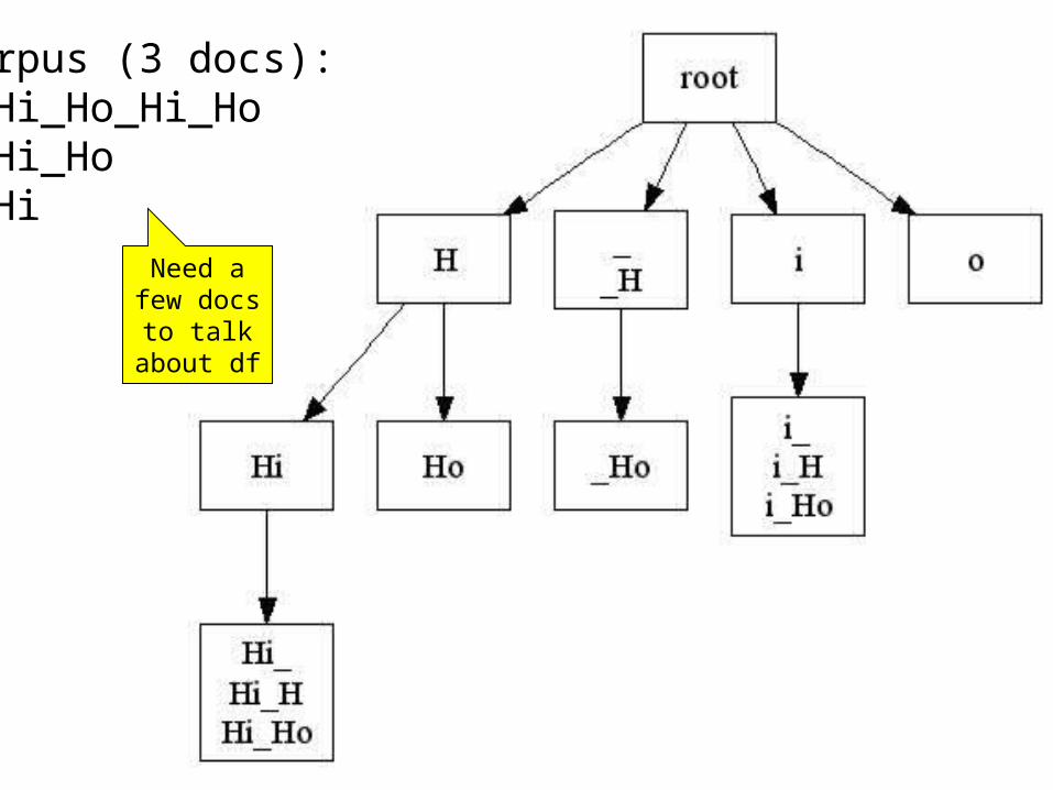
Corpus (3 docs):1. Hi_Ho_Hi_Ho2. Hi_Ho3. Hi
Need a few docs
to talk about df
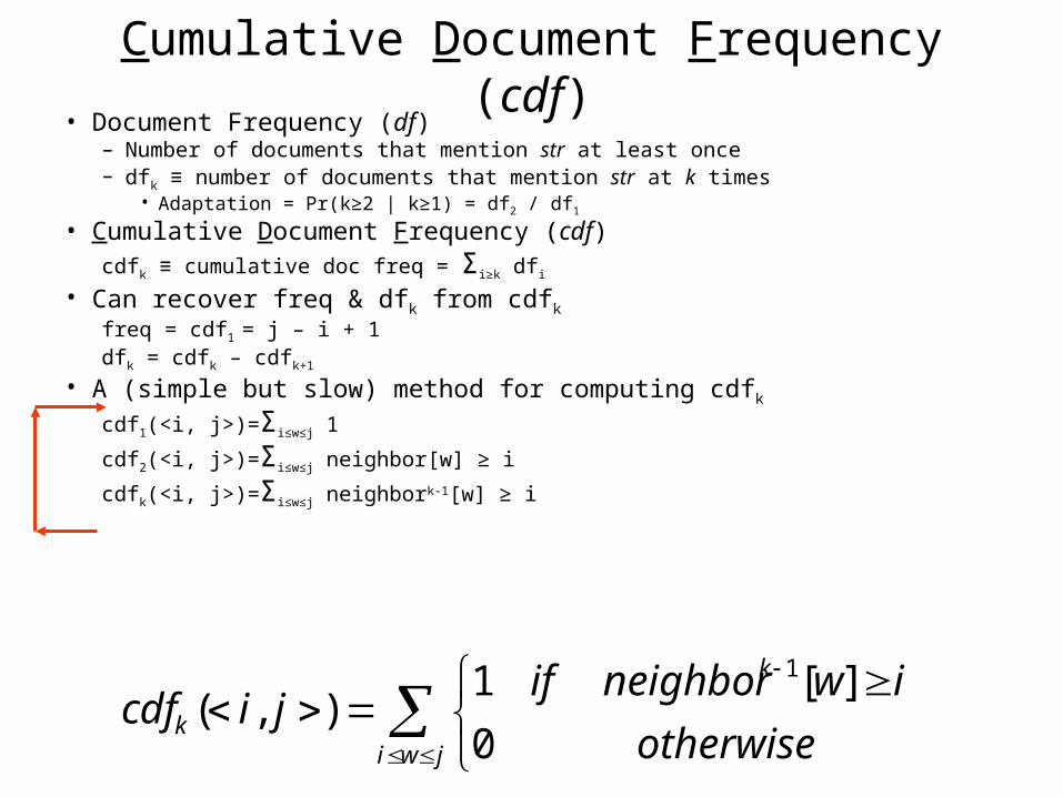
Cumulative Document Frequency (cdf)• Document Frequency (df)
– Number of documents that mention str at least once– dfk ≡ number of documents that mention str at k times
• Adaptation = Pr(k≥2 | k≥1) = df2 / df1
• Cumulative Document Frequency (cdf)cdfk ≡ cumulative doc freq = Σi≥k dfi
• Can recover freq & dfk from cdfk
freq = cdf1 = j – i + 1dfk = cdfk – cdfk+1
• A (simple but slow) method for computing cdfk
cdf1(<i, j>)=Σi≤w≤j 1
cdf2(<i, j>)=Σi≤w≤j neighbor[w] ≥ i
cdfk(<i, j>)=Σi≤w≤j neighbork-1[w] ≥ i
jwi
k
kotherwise
iwneighborifjicdf
0
][1),(
1
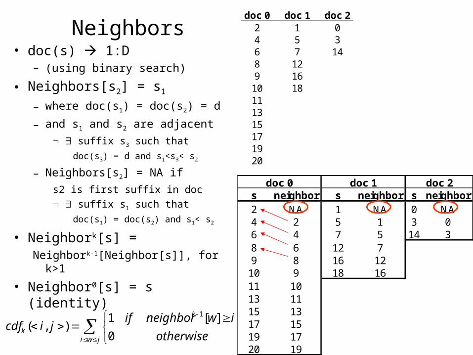
Neighbors• doc(s) 1:D
– (using binary search)
• Neighbors[s2] = s1
– where doc(s1) = doc(s2) = d
– and s1 and s2 are adjacent
suffix s3 such that
doc(s3) = d and s1<s3< s2
– Neighbors[s2] = NA if
s2 is first suffix in doc
suffix s1 such that
doc(s1) = doc(s2) and s1< s2
• Neighbork[s] = Neighbork-1[Neighbor[s]], for k>1
• Neighbor0[s] = s (identity)
doc 0 doc 1 doc 22 1 04 5 36 7 148 129 16
10 18111315171920
s neighbor s neighbor s neighbor2 NA 1 NA 0 NA4 2 5 1 3 06 4 7 5 14 38 6 12 79 8 16 12
10 9 18 1611 1013 1115 1317 1519 1720 19
doc 0 doc 1 doc 2
jwi
k
kotherwise
iwneighborifjicdf
0
][1),(
1
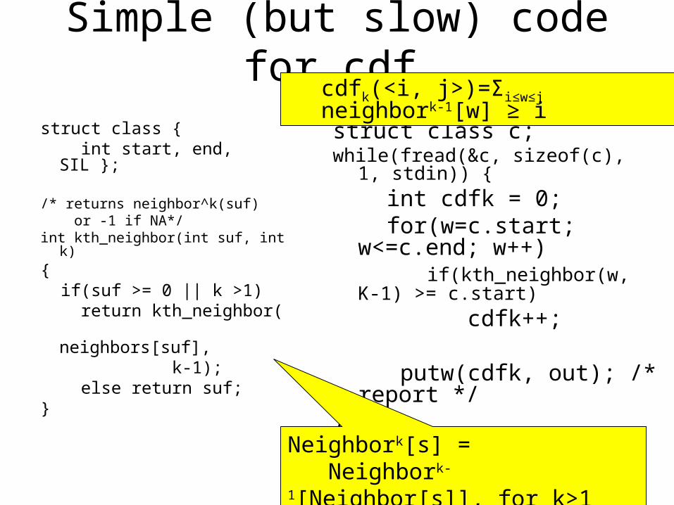
Simple (but slow) code for cdfk
struct class { int start, end, SIL };
/* returns neighbor^k(suf) or -1 if NA*/int kth_neighbor(int suf, int k)
{ if(suf >= 0 || k >1) return kth_neighbor( neighbors[suf], k-1); else return suf; }
struct class c;while(fread(&c, sizeof(c), 1, stdin)) {
int cdfk = 0; for(w=c.start; w<=c.end; w++) if(kth_neighbor(w, K-1) >= c.start)
cdfk++;
putw(cdfk, out); /* report */}
Neighbork[s] = Neighbork-1[Neighbor[s]], for k>1
cdfk(<i, j>)=Σi≤w≤j neighbork-1[w] ≥ i
cdfk(<i, j>)=Σi≤w≤j neighbork-1[w] ≥ i
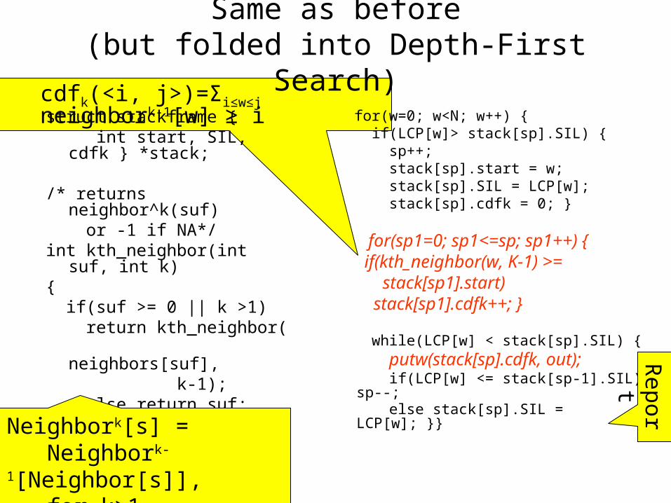
Same as before(but folded into Depth-First Search)
struct stackframe { int start, SIL, cdfk } *stack;
/* returns neighbor^k(suf) or -1 if NA*/int kth_neighbor(int suf, int k){ if(suf >= 0 || k >1) return kth_neighbor( neighbors[suf], k-1); else return suf; }
for(w=0; w<N; w++) { if(LCP[w]> stack[sp].SIL) { sp++; stack[sp].start = w; stack[sp].SIL = LCP[w]; stack[sp].cdfk = 0; }
for(sp1=0; sp1<=sp; sp1++) { if(kth_neighbor(w, K-1) >= stack[sp1].start) stack[sp1].cdfk++; }
while(LCP[w] < stack[sp].SIL) { putw(stack[sp].cdfk, out); if(LCP[w] <= stack[sp-1].SIL) sp--; else stack[sp].SIL = LCP[w]; }}
Neighbork[s] = Neighbork-1[Neighbor[s]], for k>1
Report
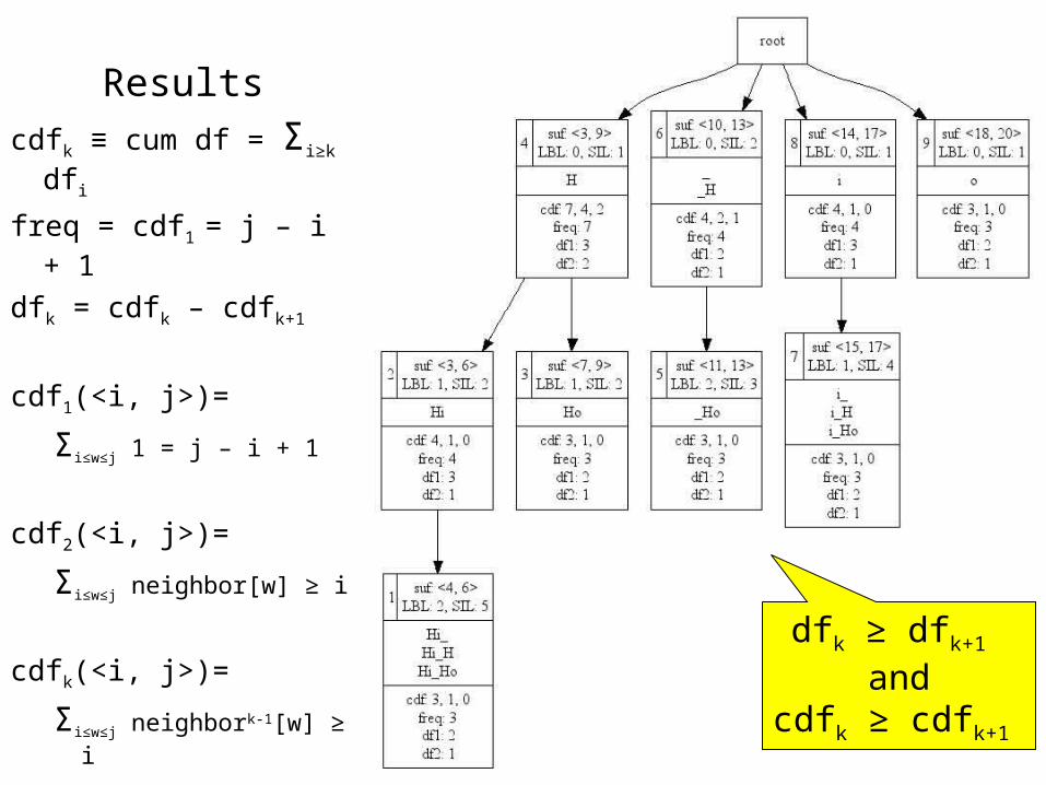
Resultscdfk ≡ cum df = Σi≥k dfi
freq = cdf1 = j – i + 1
dfk = cdfk – cdfk+1
cdf1(<i, j>)=
Σi≤w≤j 1 = j – i + 1
cdf2(<i, j>)=
Σi≤w≤j neighbor[w] ≥ i
cdfk(<i, j>)=
Σi≤w≤j neighbork-1[w] ≥ i
dfk ≥ dfk+1 and
cdfk ≥ cdfk+1
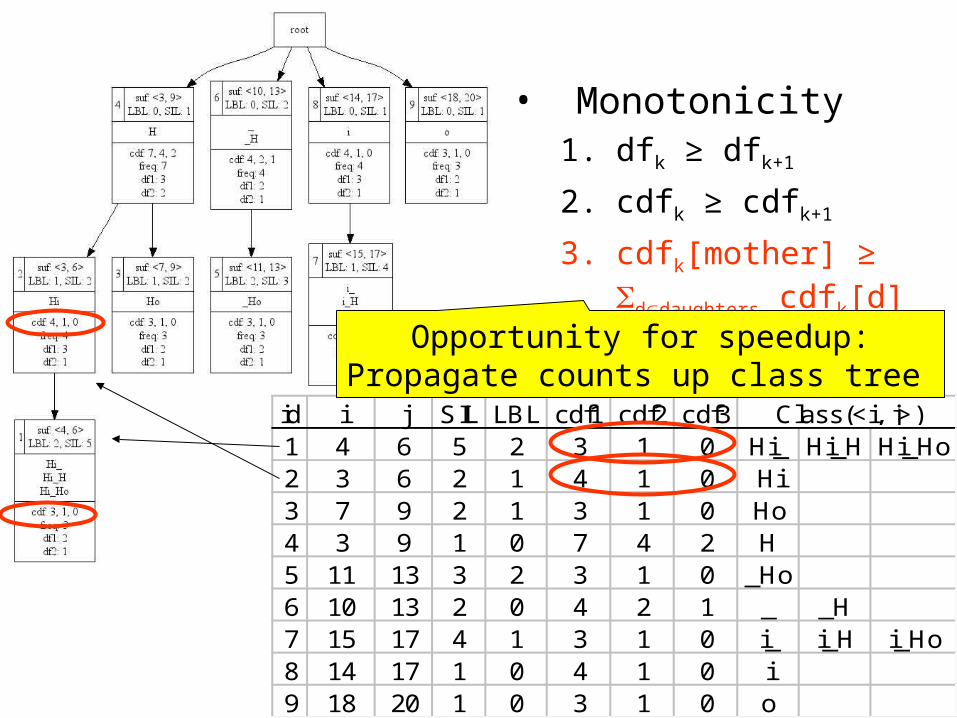
• Monotonicity1. dfk ≥ dfk+1
2. cdfk ≥ cdfk+1
3. cdfk[mother] ≥ ddaughters cdfk[d]
id i j SIL LBL cdf1 cdf2 cdf31 4 6 5 2 3 1 0 Hi_ Hi_H Hi_Ho2 3 6 2 1 4 1 0 Hi3 7 9 2 1 3 1 0 Ho4 3 9 1 0 7 4 2 H5 11 13 3 2 3 1 0 _Ho6 10 13 2 0 4 2 1 _ _H7 15 17 4 1 3 1 0 i_ i_H i_Ho8 14 17 1 0 4 1 0 i9 18 20 1 0 3 1 0 o
Class(<i, j>)
Opportunity for speedup:Propagate counts up class tree
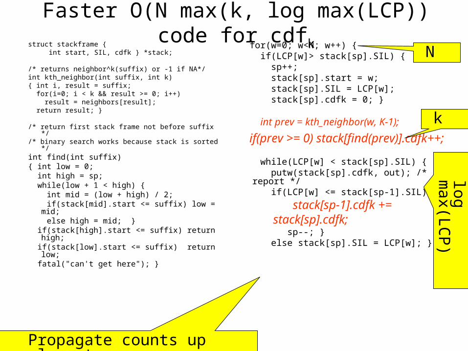
Faster O(N max(k, log max(LCP)) code for cdfkstruct stackframe { int start, SIL, cdfk } *stack;
/* returns neighbor^k(suffix) or -1 if NA*/int kth_neighbor(int suffix, int k){ int i, result = suffix; for(i=0; i < k && result >= 0; i++) result = neighbors[result]; return result; }
/* return first stack frame not before suffix *//* binary search works because stack is sorted */int find(int suffix){ int low = 0; int high = sp; while(low + 1 < high) { int mid = (low + high) / 2; if(stack[mid].start <= suffix) low = mid; else high = mid; } if(stack[high].start <= suffix) return high; if(stack[low].start <= suffix) return low; fatal("can't get here"); }
for(w=0; w<N; w++) { if(LCP[w]> stack[sp].SIL) { sp++; stack[sp].start = w; stack[sp].SIL = LCP[w]; stack[sp].cdfk = 0; }
int prev = kth_neighbor(w, K-1);
if(prev >= 0) stack[find(prev)].cdfk++;
while(LCP[w] < stack[sp].SIL) { putw(stack[sp].cdfk, out); /* report */ if(LCP[w] <= stack[sp-1].SIL) {
stack[sp-1].cdfk += stack[sp].cdfk; sp--; } else stack[sp].SIL = LCP[w]; }}
Propagate counts up class tree
log max(LC
P)
N
k
Substring StatisticsOutline
• Goal: Substring Statistics– Words Substrings (Ngrams)– Anything we do with words,
• we should be able to do with substrings (ngrams)…
– Stats• freq(str) and location
(sufconc), • df(str), dfk(str), jdf(str1, str2)• and combinations thereof
• Suffix Arrays & LCP• Classes: One str All strs
– N2 substrings N classes– Class(<i,j>) = { str | str starts
every suffix in interval and no others }
– Compute stats over classes
• DFS Traversal of Class Tree• Cumulative Document
frequency (cdfk)– freq = cdf1
– dfk = cdfk – cdfk+1
• Neighbors
• Cross Validation• Joint Document Freq
– Sketches
• Apps
jwi
k
kotherwise
iwneighborifjicdf
0
][1),(
1
We are here
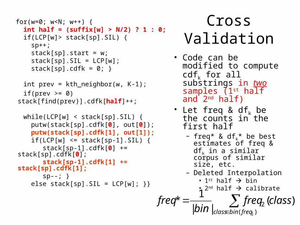
Cross Validation
• Code can be modified to compute cdfk for all substrings in two samples (1st half and 2nd half)
• Let freq & dfk be the counts in the first half– freq* & dfk* be best
estimates of freq & dfk in a similar corpus of similar size, etc.
– Deleted Interpolation• 1st half bin• 2nd half calibrate
for(w=0; w<N; w++) { int half = (suffix[w] > N/2) ? 1 : 0; if(LCP[w]> stack[sp].SIL) { sp++; stack[sp].start = w; stack[sp].SIL = LCP[w]; stack[sp].cdfk = 0; }
int prev = kth_neighbor(w, K-1);
if(prev >= 0) stack[find(prev)].cdfk[half]++; while(LCP[w] < stack[sp].SIL) { putw(stack[sp].cdfk[0], out[0]); putw(stack[sp].cdfk[1], out[1]); if(LCP[w] <= stack[sp-1].SIL) { stack[sp-1].cdfk[0] += stack[sp].cdfk[0]; stack[sp-1].cdfk[1] += stack[sp].cdfk[1]; sp--; } else stack[sp].SIL = LCP[w]; }}
)(
2
1
)(||
1*
freqbinclass
classfreqbin
freq
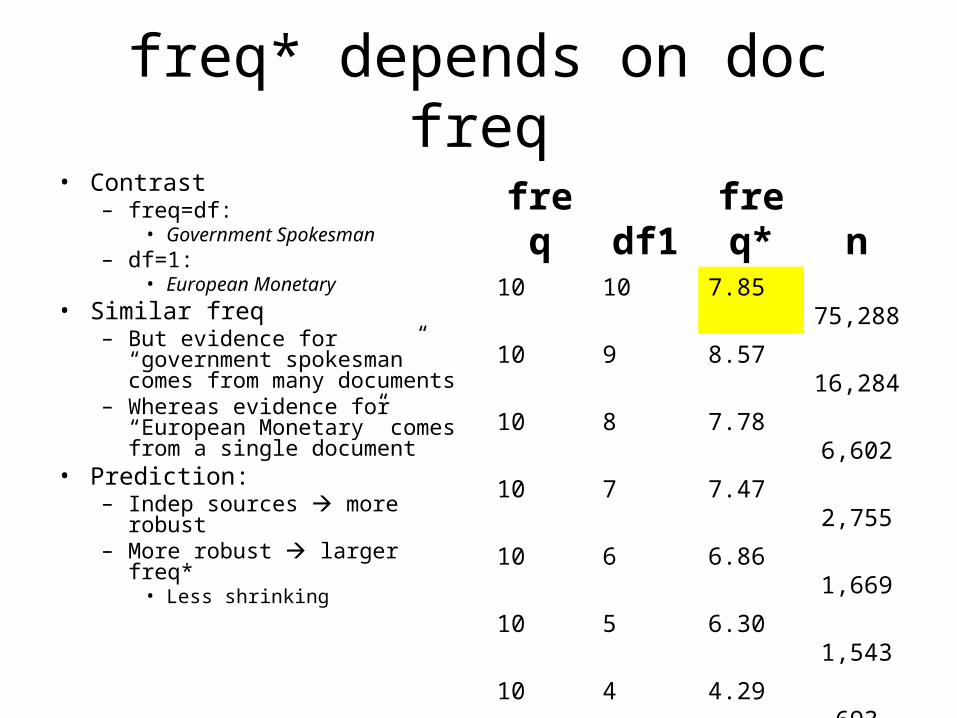
freq* depends on doc freq• Contrast
– freq=df:• Government Spokesman
– df=1:• European Monetary
• Similar freq– But evidence for “government
spokesman” comes from many documents
– Whereas evidence for “European Monetary” comes from a single document
• Prediction:– Indep sources more robust– More robust larger freq*
• Less shrinking
freq df1 freq* n10 10 7.85 75,288
10 9 8.57 16,284
10 8 7.78 6,602
10 7 7.47 2,755
10 6 6.86 1,669
10 5 6.30 1,543
10 4 4.29 693
10 2 4.42 509
10 3 3.93 416
10 1 2.87 282
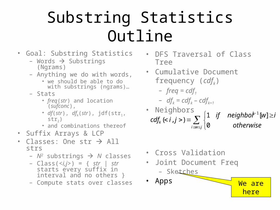
Substring StatisticsOutline
• Goal: Substring Statistics– Words Substrings (Ngrams)– Anything we do with words,
• we should be able to do with substrings (ngrams)…
– Stats• freq(str) and location
(sufconc), • df(str), dfk(str), jdf(str1, str2)• and combinations thereof
• Suffix Arrays & LCP• Classes: One str All strs
– N2 substrings N classes– Class(<i,j>) = { str | str starts
every suffix in interval and no others }
– Compute stats over classes
• DFS Traversal of Class Tree• Cumulative Document
frequency (cdfk)– freq = cdf1
– dfk = cdfk – cdfk+1
• Neighbors
• Cross Validation• Joint Document Freq
– Sketches
• Apps
jwi
k
kotherwise
iwneighborifjicdf
0
][1),(
1
We are here
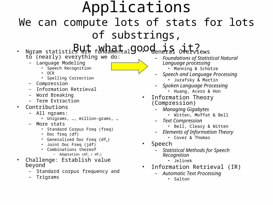
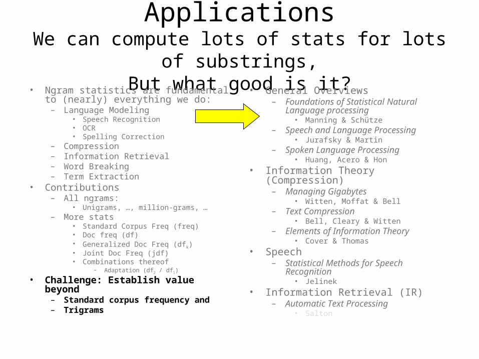
ApplicationsWe can compute lots of stats for lots of substrings,
But what good is it?• Ngram statistics are fundamental to
(nearly) everything we do:– Language Modeling
• Speech Recognition• OCR• Spelling Correction
– Compression– Information Retrieval– Word Breaking– Term Extraction
• Contributions– All ngrams:
• Unigrams, …, million-grams, …– More stats
• Standard Corpus Freq (freq)• Doc freq (df)• Generalized Doc Freq (dfk)• Joint Doc Freq (jdf)• Combinations thereof
– Adaptation (df2 / df1)
• Challenge: Establish value beyond– Standard corpus frequency and – Trigrams
• General Overviews– Foundations of Statistical Natural
Language processing• Manning & Schütze
– Speech and Language Processing• Jurafsky & Martin
– Spoken Language Processing• Huang, Acero & Hon
• Information Theory (Compression)– Managing Gigabytes
• Witten, Moffat & Bell– Text Compression
• Bell, Cleary & Witten– Elements of Information Theory
• Cover & Thomas
• Speech– Statistical Methods for Speech
Recognition• Jelinek
• Information Retrieval (IR)– Automatic Text Processing
• Salton
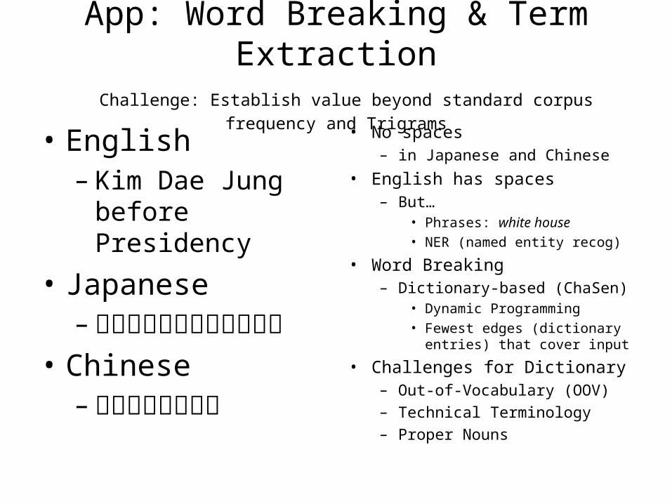
App: Word Breaking & Term Extraction Challenge: Establish value beyond standard corpus frequency and Trigrams
• English– Kim Dae Jung
before Presidency
• Japanese– 大統領になる以前
の金大中• Chinese
–未上任前的金大中
• No spaces– in Japanese and Chinese
• English has spaces– But…
• Phrases: white house• NER (named entity recog)
• Word Breaking– Dictionary-based (ChaSen)
• Dynamic Programming• Fewest edges (dictionary
entries) that cover input
• Challenges for Dictionary– Out-of-Vocabulary (OOV)– Technical Terminology– Proper Nouns
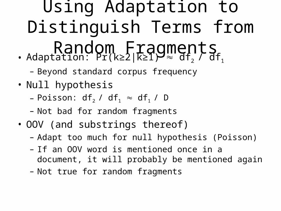
Using Adaptation to Distinguish Terms from Random Fragments • Adaptation: Pr(k≥2|k≥1) df2 / df1
– Beyond standard corpus frequency
• Null hypothesis– Poisson: df2 / df1 df1 / D
– Not bad for random fragments
• OOV (and substrings thereof)– Adapt too much for null hypothesis (Poisson)– If an OOV word is mentioned once in a document, it
will probably be mentioned again– Not true for random fragments
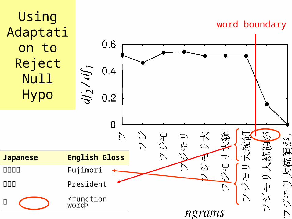
Using Adaptation to Reject Null Hypo
Japanese English Gloss
フジモリ Fujimori
大統領 President
が <function word>
word boundary
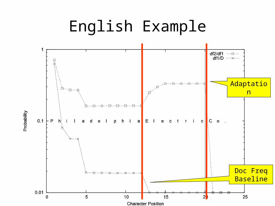
English Example
Adaptation
Doc FreqBaseline
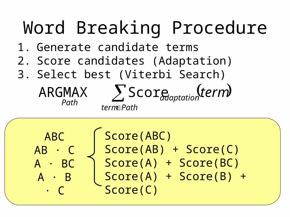
Word Breaking Procedure1. Generate candidate terms2. Score candidates (Adaptation)3. Select best (Viterbi Search)
Score(ABC)Score(AB) + Score(C)Score(A) + Score(BC)Score(A) + Score(B) + Score(C)
ABCAB ∙ CA ∙ BCA ∙ B ∙ C
Pathterm
adaptationPath
termScoreARGMAX
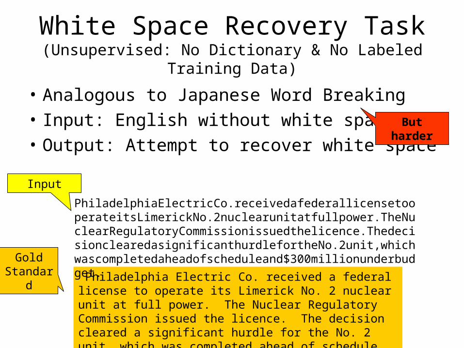
White Space Recovery Task(Unsupervised: No Dictionary & No Labeled Training Data)
• Analogous to Japanese Word Breaking
• Input: English without white space
• Output: Attempt to recover white space
Philadelphia Electric Co. received a federal license to operate its Limerick No. 2 nuclear unit at full power. The Nuclear Regulatory Commission issued the licence. The decision cleared a significant hurdle for the No. 2 unit, which was completed ahead of schedule and $300 million under budget.
PhiladelphiaElectricCo.receivedafederallicensetooperateitsLimerickNo.2nuclearunitatfullpower.TheNuclearRegulatoryCommissionissuedthelicence.ThedecisionclearedasignificanthurdlefortheNo.2unit,whichwascompletedaheadofscheduleand$300millionunderbudget.
Input
Gold Standard
But harder
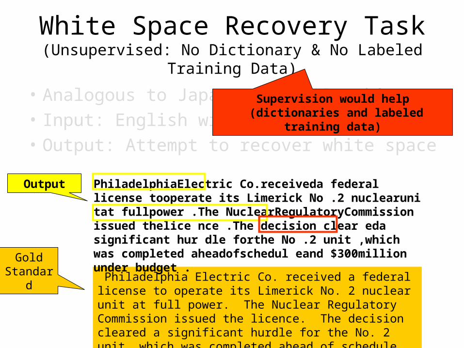
White Space Recovery Task(Unsupervised: No Dictionary & No Labeled Training Data)
• Analogous to Japanese Word Breaking
• Input: English without white space
• Output: Attempt to recover white space
Philadelphia Electric Co. received a federal license to operate its Limerick No. 2 nuclear unit at full power. The Nuclear Regulatory Commission issued the licence. The decision cleared a significant hurdle for the No. 2 unit, which was completed ahead of schedule and $300 million under budget.
Output
Gold Standard
PhiladelphiaElectric Co.receiveda federal license tooperate its Limerick No .2 nuclearuni tat fullpower .The NuclearRegulatoryCommission issued thelice nce .The decision clear eda significant hur dle forthe No .2 unit ,which was completed aheadofschedul eand $300million under budget .
Supervision would help (dictionaries and labeled training data)
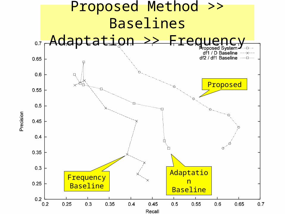
Proposed Method >> BaselinesAdaptation >> Frequency
Proposed
Adaptation BaselineFrequency
Baseline
ApplicationsWe can compute lots of stats for lots of substrings,
But what good is it?• Ngram statistics are fundamental to
(nearly) everything we do:– Language Modeling
• Speech Recognition• OCR• Spelling Correction
– Compression– Information Retrieval– Word Breaking– Term Extraction
• Contributions– All ngrams:
• Unigrams, …, million-grams, …– More stats
• Standard Corpus Freq (freq)• Doc freq (df)• Generalized Doc Freq (dfk)• Joint Doc Freq (jdf)• Combinations thereof
– Adaptation (df2 / df1)
• Challenge: Establish value beyond– Standard corpus frequency and – Trigrams
• General Overviews– Foundations of Statistical Natural
Language processing• Manning & Schütze
– Speech and Language Processing• Jurafsky & Martin
– Spoken Language Processing• Huang, Acero & Hon
• Information Theory (Compression)– Managing Gigabytes
• Witten, Moffat & Bell– Text Compression
• Bell, Cleary & Witten– Elements of Information Theory
• Cover & Thomas
• Speech– Statistical Methods for Speech
Recognition• Jelinek
• Information Retrieval (IR)– Automatic Text Processing
• Salton
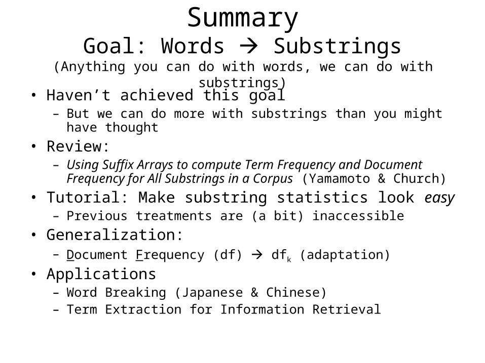
SummaryGoal: Words Substrings
(Anything you can do with words, we can do with substrings)
• Haven’t achieved this goal– But we can do more with substrings than you might have thought
• Review: – Using Suffix Arrays to compute Term Frequency and Document
Frequency for All Substrings in a Corpus (Yamamoto & Church)
• Tutorial: Make substring statistics look easy– Previous treatments are (a bit) inaccessible
• Generalization: – Document Frequency (df) dfk (adaptation)
• Applications– Word Breaking (Japanese & Chinese)– Term Extraction for Information Retrieval
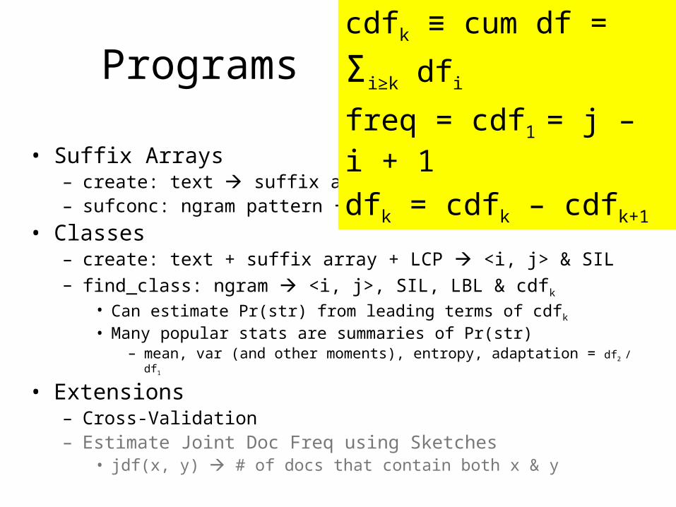
Programs
• Suffix Arrays– create: text suffix array & LCP vector– sufconc: ngram pattern freq & location
• Classes– create: text + suffix array + LCP <i, j> & SIL– find_class: ngram <i, j>, SIL, LBL & cdfk
• Can estimate Pr(str) from leading terms of cdfk
• Many popular stats are summaries of Pr(str)– mean, var (and other moments), entropy, adaptation = df2 / df1
• Extensions– Cross-Validation– Estimate Joint Doc Freq using Sketches
• jdf(x, y) # of docs that contain both x & y
cdfk ≡ cum df = Σi≥k dfi
freq = cdf1 = j – i + 1
dfk = cdfk – cdfk+1


![Melissa Chase and Emily Shen Substring ...Substring-SearchableSymmetricEncryption 265 45] propose schemes that allow updates to the stored documents, and Kurosawa and Ohtaki [38] propose](https://img.pdfslide.us/doc/110x75/5e6975b7bb7b2f2a5b023843/melissa-chase-and-emily-shen-substring-substring-searchablesymmetricencryption.jpg)