Substitution Among Charitable Contributions: An Experimental Study

David Reinstein

Abstract

The question of whether charitable gifts are complements or substitutes, and the extent to which charities arerivals, is unresolved in the economic literature. The answer is relevant to charities and policymakers, as wellas to economic models of altruism. Identifying this using observational data is difficult: there is a lack ofclear independent price variation and few observable shocks that can be claimed to specifically affect givingto one charity. I implement such variation in a laboratory setting: in a series of stages, subjects may donateto a varying set of one to four charities, with “prices” (defined as the inverse of one minus the rate at which Isupplement contributions,i.e., the cost of passing a dollar to the charity) and promotional information varyingby stage, subject, and charity. All of the specific shocks strongly increase giving to the targeted charities,and this leads to decreased giving to the charities not targeted; I interpret this as a form of crowding-out. Instandard economic terms, subjects exhibit price-elastic demand and positive cross-price elasticities betweencharities, particularly when the charities serve similar goals. Overall, this evidence suggests that “expendituresubstitution” between charities may be important in some real-world environments.

Preprint submitted to Elsevier May 25, 2012

1. Introduction

In modeling philanthropic giving, economists have typically focused on two major issues: the crowding outof government grants and the impact of different tax regimes on overall giving. Little attention has been givento the extent to which an individual’s contribution to one cause comes at the expense of her other philanthropy.This issue has come to the attention of policy-makers and journalists in the wake of the September 11, 2001terrorist attacks,1 and again after the 2004 Indian Ocean tsunami2 and 2005’s Hurricane Katrina3 – in eachcase there was a concern that the flood of donations to the well-publicized cause would dampen giving to othercharities. However, some have dismissed this concern, claiming that “donor fatigue” is a myth.4

This paper presents the results of experiments designed to elicit preferences over charitable contributions.More specifically, I measure whether and to what extent an individual’s contribution to one cause comes at theexpense of his or her other philanthropy. I first present this substitution in terms of the cross-derivatives andcross-elasticities of expenditure on charitable gifts, in response to changes in the effective price5 of giving to acharity and other “specific” shocks, and discuss the ratios of these responses. I next examine the relationshipbetween the change in giving to one charity, in response to a specific shock, and the change in giving to the“un-shocked” charities; this offers suggestive evidence of “expenditure substitution.” . The nature of this re-lationship is of great popular interest and is crucial to tax and social spending policy, nonprofit management,and individual ethical decision-making (see Reinstein, 2011 for further motivation). It is also important tothe economic literature for at least two reasons. First, it complicates the estimation, and the normative im-plications, of the price-elasticity of giving and the crowding out of government spending. Second, knowingwhether expenditure substitution occurs, whether it is complete (i.e., one-for-one), and how it depends on thecharities compared can offer evidence against or in support of several proposed economic models of giving,including the public goods (Becker, 1974), warm-glow (Andreoni, 1990), tithing, and Kantian (Sugden, 1982)models.6

Observational data on charitable giving (e.g., survey data or tax data) offers few variables that can beused to identify “specific” shocks – shocks that alter giving to one charity but have no independent effect ongiving to other charities. Most observable variables that are believed to increase giving to one charity willalso increase giving to other charities, masking substitution effects. Experiments can offer complementaryevidence for substitution patterns that are not vulnerable to such endogeneity – we can manipulate the priceof giving to one charity independently of the price of other gifts, and can introduce other specific shocks.

While there has been a great deal of laboratory and field experimentation involving charitable giving inrecent years (see section 2), few allow gifts to multiple charities, and none examine substitution patterns

1<http://www.sptimes.com/2002/09/04/911/Sept_11_donations_swa.shtml>2<http://www.cnn.com/2005/WORLD/africa/07/30/africa.hungry.ap/index.html>3“Katrina Giving Cuts Donations To Other Groups; As Relief Contributions Pour In, Unrelated Charities Retool Plans To Get Back

on Donors’ Minds” – The Wall Street Journal, September 20, 2005.In response, the government increased the maximum allowable tax deduction for charitable giving to 100 percent of income

on donations made during the last part of 2005. – “Katrina Emergency Tax Relief Act...,” by Candace Clark, UNC-Chapel Hill.<http://www.johnbrownlimited.com/newsletter/1005/index.cfm>

4“Many Dismissing ‘Donor Fatigue’ as Myth”– New York Times, April 30, 20065The issue of defining “price” in charitable giving is difficult; here I consider the amount an individual must sacrifice in order to

augment the charity’s income by one dollar. However, other interpretations could be considered, taking into account the percievedrelative effectiveness of the charities in pursuing their goals or increase the utility of the

6See Reinstein (2011) for a further discussion of these models and their predictions.

2

between gifts. As in Eckel and Grossman (2003) (henceforth EG), my experiment is essentially a modifieddictator game, in which subjects “make a series of allocation decisions, dividing an endowment betweenthemselves and their chosen charities.” An ideal experiment would exogenously shift the amount allocatedto one good and observe the resulting reallocation of the other choices. However, the consumption valueof charitable giving to the donor, including benefits such as warm-glow (Andreoni, 1990) and self-signaling(e.g., Benabou and Tirole, 2003) may depend on the gift being voluntary. Instead of forcing participants tochange their giving decisions, I generate “shocks” that are intended to specifically affect one type of giving,and I observe the resulting giving to this charity and to other charities.

I ran two comparable but distinct waves of experiments, each wave containing three sessions, using a totalof 97 subjects, mainly U.C. Berkeley students, but also including some staff and alumni. I give a detaileddescription of each experimental run in section 4. In each experiment, each subject makes his or her decisionsin a sequence of stages. At the end of the experiment, one stage is randomly drawn, and the outcome of thisstage (a payment to the subject and/or the charities) is realized. Each experiment involves a “baseline” stage,where a subject can donate up to their entire endowment to one or more of three charities, and are informedthat the experimenters will supplement each of their gifts by 20%, i.e. a 20% “match rate”, to induce subjectsto give within the lab rather than wait to decide later. The subjects can keep what they do not donate. As“baseline” charities I chose CARE-USA, an NGO that supports international development and disaster relief,Medical Research Charities, a fund that benefits an array of medical research institutions, and ScholarshipAmerica, which offers university scholarships to underprivileged US youths.7

In addition to the baseline stage, the treatment stages (“shocks”) involve restricting the choice set to onecharity, augmenting the choice set to include other charities (UNICEF and The Nature Conservancy), signifi-cantly increasing the match rate for one of the charities, and showing a promotional video. Nearly all of theseshocks had the hypothesized effect on gifts. The subjects exhibit (locally) price-elastic demand – a highermatch rate, and thus a lower effective price of putting a dollar in the charity’s pocket lead subjects to spendmore of their endowment on gifts to that charity (i.e., increase donations even without counting the matchedamounts).

While subjects’ behavior is heterogeneous, my results strongly suggest that these charities are substitutesin this context. When a shock leads subjects to increase their giving to one charity they are far more likely todecrease their giving to the other (unshocked) charities than to increase this giving. In structural regressionsI consistently find a large own-price expenditure elasticity,8 and large positive and significant cross-priceeffects. In direct 2sls regressions of giving to one charity on giving to another, where the latter is instrumentedby the shocks mentioned above, I find significant “crowding out.”9 The crowding out is even stronger for thetwo charities that have the most similar goals: UNICEF and CARE. My numerical estimates are not intendedas accurate measures of real-world substitution; rather, the experimental evidence is meant to reveal overallpatterns of behavior, and complements the observational results in Reinstein (2011).

7These were chosen to resemble the categories “Basic needs,” “Health,” and “Education” in the Panel Survey of Income Dynamics(PSID/COPPS) data, so the results could be broadly compared to Reinstein (2011).

8I refer to expenditure elasticities since I speak of the amount of income the subjects sacrifice, rather than the amount the charityreceives after our match contributions.

9In the linear 2sls regression I find crowding out at a 37% rate; as this includes observations where one donation goes to zero, the“conditional on positive” effect is higher (Tobit estimates available by request).

3

In section 2 I survey previous experiments examining charitable giving, both in a laboratory context andin natural settings. Section 3 discusses a simple model of giving and identifies the object of my estimation.In section 4 I describe my experiment and procedures. Section 5 presents the main results, both on thesubstitution patterns and on direct effects of treatments, presenting results from a standard structural regressionand from direct measures of expenditure substitution. In section 6 I discuss internal validity and externalgeneralizability, testing for robustness against alternative hypotheses. I conclude in section 7.

2. Literature Review

There is a paucity of theoretical, empirical observational, or experimental work on substitution patternsbetween charitable gifts or on the cross-price elasticities between charities. Prominent theoretical work ongiving (e.g., Becker, 1974; Andreoni, 1990; Harbaugh, 1998; Glazer and Konrad, 1996; and Duncan, 2004)models an individual’s charitable giving and public goods contributions as a single aggregate, and does notexplicitly differentiate between gifts to different charitable causes. Still, these models can be generalized toyield varying predictions for expenditure substitution; this is analyzed in Reinstein (2011). The competitionbetween charities has been discussed by Bilodeau and Slivinski (1997), Chua and Ming Wong (2003), andothers.

Observational empirical work has focused on a few key policy issues, particularly attempting to estimatethe (after-tax) price elasticity of charitable giving, and the “crowding out” of government spending.10

Economists have run numerous experiments investigating motivations for other-regarding behavior andcharitable giving, but few have investigated choices between multiple charities. EG (1996; 1998; 2003; 2006)conduct several laboratory studies involving actual charitable giving. Their 1996 paper extended the literatureon double-anonymous dictator experiments to argue that altruism motivates behavior, but “fairness and altru-ism require context” – they find that laboratory contributions to an established charity are much higher thancontributions to an anonymous fellow student.

Several papers have also used field experiments to examine charitable giving in a natural setting. Frey andMeier (2004), Karlan and List (2007), and Rasul and Huck (2010) test the effect of matching mechanismson donations in field experiments, finding mixed evidence on their effectiveness in increasing contributions.Other experimental or quasi-experimental research have examined various social and reputational influenceson giving behavior (Alpizar et al., 2008; Shang and Croson, 2005; Carman, 2003; Soetevent, 2005; Martin andRandall, 2008); the crowding out effects of public funding (Bolton and Katok, 1998), the prestige motivationfor giving (Harbaugh, 1998), and fund-raising techniques and psychology/behavior (Weyant, 1996; List andLucking-Reiley, 2002; Falk, 2004 Karlan and List, 2007; Soetevent, 2005 Fisman et al., 2005; Andreoni andMiller, 2002.) Some recent work has begun to address issues closely related to the present paper. Van Diepenet al. (2009) offer some field experimental evidence on the crowding-out effects of direct mail solicitations.Borgloh (2009) investigated the impact of the German church tax on households’ other charitable giving.Null (2011) used a field experiment to examine how donations to different charities respond to changes inrelative match rates – however, as the total donation was decided ex-ante, the substitution among charities wasconstrained to be complete. Finally, an earlier work (Andreoni et al., 1996) examines substitution between

10For more complete surveys of the literature, see Andreoni (2006a), Sargeant and Woodliffe (2007), or Bekkers and Wiepking (2008).

4

giving and volunteering. However, to the best of my knowledge, no work directly addresses the cross-priceelasticity (nor the expenditure substitution) between gifts to charitable causes.

3. Conceptual Framework

Americans have donated more than $1 billion to the [Katrina/ flooding] relief ... But thelargess is starting to come at the expense of charities with other missions. ...The challenge ispeople like Betty and Larry Sullivan .... the couple has given $4,000 for the tsunami relief effortand some $35,000 to help Hurricane Katrina survivors ... As for donations to other charities thisyear, “That’s history,” says Mrs. Sullivan.11

In this section I offer a framework for understanding the “expenditure substitution” that I estimate, and itsrelationship to price effects, specific shock effects, and observables. 12 Economists frame demand, includingdemand for making charitable gifts, as a simultaneous decision to purchase a bundle of goods and servicesto maximize a utility function subject to a budget constraint. In this framework, parameters that affect theutility function (e.g., good weather) and the budget constraint (income and prices) are said to impact all of theconsumption choices – these exogenous parameters are not seen as specific to any good. We typically estimate(e.g.) own and cross-price derivatives and elasticities, as I do in section 5.3. To ask “how does consumption ofA affect consumption of B?” is not meaningful: we cannot assert causality for such simultaneous decisions,and the ratios of changes in these choices will depend on what is causing the changes.13 However, as seen inthe quotes above, non-economists often pose this question, frequently make their decisions sequentially, andconceive of one purchase coming at the expense of another. Can we argue that an event such as the Tsunamihas a direct impact only on gifts to one cause, and not other causes? In the standard economic framework thisstatement is not coherent. A shock “a ” can be specific in that it only changes the marginal utility of gifts toone cause, as in equation 1 below, but if decisions are simultaneous, the shock will affect all choices. Thealtruistic consumer’s utility can be represented as

U = f (x,g1,h(g2,a)) (1)

e.g., f (x,g1,g2 �a) (2)

where f is a composite function representing the consumer’s utility as a function of x, the numeraire good(own consumption), and the charitable gifts. g1 and g2 are gifts to distinct charities (the amount received bythe charities as a result of the consumer’s gift), and a represents a specific shock to the marginal utility of thesecond type of charitable gift. Thus a affects utility only through the h() function. If a policy-maker wantsto predict the impact of the shock a on gifts to “unshocked” charities g1, having an estimate of the effect ong2 may be useful in assessing the magnitude of the shock. A policy-maker or charity may know there was atsunami and also observe measures of disaster giving in response, and may want to predict or infer the likely

11The Wall Street Journal, September 20, 2005.12The model is presented not to derive new results but to identify and explain what I am seeking to estimate.13However, even our technical economic terms, although defined in terms of cross-price elasticities, suggest a more direct causation:

coffee “substitutes for” tea, while cream “complements” both beverages.

5

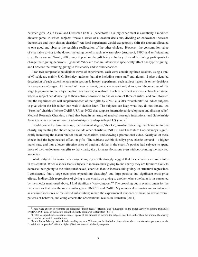
Figure 1: Timeline of experiments

impact on another set of charities. Furthermore, under some plausible conditions (discussed in appendix 8.1)the substitution response to any shock will be a predictable function of the “direct” impact of the shock (above,on g2).

4. Experimental Procedures and Design

14

4.1. Procedures

My experiment was run using the Experimental Social Science Laboratory (X-Lab) at the Universityof California, Berkeley.15 Subjects were recruited by the X-Lab (those interested are put on an email listand informed about opportunities to participate) from a wide pool of students and staff at the University ofCalifornia, Berkeley. None of the subjects were allowed to participate in my experiment more than once,although many had taken part in X-Lab experiments run by other researchers. The experiments involved 97subjects in total. In the first two sessions, subjects were given a $5 show-up fee. In the third session I offereda larger ($8) base payment (to help recruit staff members), while in the second wave (sessions 4-6) the basepayments were again $5.

In order to test for a variety of effects and include different robustness checks, I implemented two exper-imental designs (henceforth “waves”); although they differ to some extent, both waves have the same overallstructure and basic focus. Six sessions of the experiment were completed:16 three runs of the first wave andthree runs of the second, as described in the timetable (figure 1) above. Each session took roughly one hour,plus about 15 minutes to record payments and to print and distribute checks.

A complete set of screenshots, as well as the software code and the complete integrated data set of exper-imental results (including decisions, survey responses, and response times) are available by request. The videoused for the wave one, stage 6 treatment can be viewed at: <http://www.care.org/videos/picture_a_world.mov.>.The first wave of experiments used the software Medialab-v4, by Empirisoft, www.empirisoft.com. The sec-ond wave was programmed and conducted with the software Z-Tree (Fischbacher, 2007). After making the

14The basics of the charitable giving experiment have been noted in the introduction. In first explain the overall procedures and detailsto put the two waves of experiments in context, and then describe the actual experimental designs in detail.

15Research was conducted under the X-Lab Master Human Subjects Protocol <http://xlab.berkeley.edu/cphs/master_protocol.pdf.>and approved by the UC Berkeley Committee for Protection of Human Subjects.

16Because of a computer failure, the first session had to be conducted via oral instruction and answers written with paper and pen, nopost-experiment survey data were collected, and assignment of a stage for payment was done by generating 20 random numbers, one foreach subject. This run was otherwise identical to that of the other sessions. The first run, although conducted under a slightly differentapparent conditions (“frames”), does not have significantly different overall levels of giving in the first three stages relative to the secondor third run.

6

choices the subjects answered a series of survey questions, and were debriefed on the purpose of the exper-iment. One of the stages was randomly selected by the computer17 for each subject, and the amounts thesubject chose to contribute and keep in that stage were recorded. After all subjects were complete, the checksto subjects were printed out and distributed with roughly a 10-15 minute delay. The subjects were paid theamount they chose to keep in the randomly chosen stage, plus the initially promised “base payment”: $5 insessions 1,2,4,5, and 6 and $8 in the third session. Within one week of each session, the X-Lab wrote a singlecheck to each of the charities equal to the amounts promised.

17In the first run, because of computer problems, I used a list of randomly generated numbers, one for each subject’s ID.

7

Experimental Design

1st waveStage Match rate Charity set. Treatment

1 Base 20% 1 stratified charity Donating is allowed to single charity only2 Base 20% 1 stratified charity Donating is allowed to single charity only3 Base 20% 1 stratified charity Donating is allowed to single charity only4 Base 20% 3 charities Donation restriction is removed5 50%- CARE-USA, other

base 20%3 charities CARE-USA price shock

6 Base 20% Full 3 charity set Promotional video CARE-USA

2nd wave1 Base 20% 3 charities2 50% for stratified, other

20% base.3 charities Varying price shock

3 50% for stratified, other20% base.

3 charities Varying price shock

4 50% for stratified, other20% base.

3 charities Varying price shock

5 Base 20% 3 charities6 Base 20% 4 charities, additional

stratifiedCharity set expanded by UNICEF or

TNC7 Base 20% 4 charities, additional

stratifiedCharity set expanded by UNICEF or

TNC8 50% for additional, other

20% base.4 charities Charity set expanded by UNICEF with

price shock9 Base 20% 3 charities Decision anonymously reported to

randomly-selected participant.10 Base 20% 3 charities11 Base 20% 3 charities Decision reported to subject to the left12 Base 20% 3 charities13 Base 20% 3 charities Decision reported to matched subject 2

to the left or right13th stage was preannounced to be final.

Three charity set consists of CARE-USA, Scholarship America and Medical Research Charities charities.

Table 1: Experimental Design

8

4.2. Design: Wave One

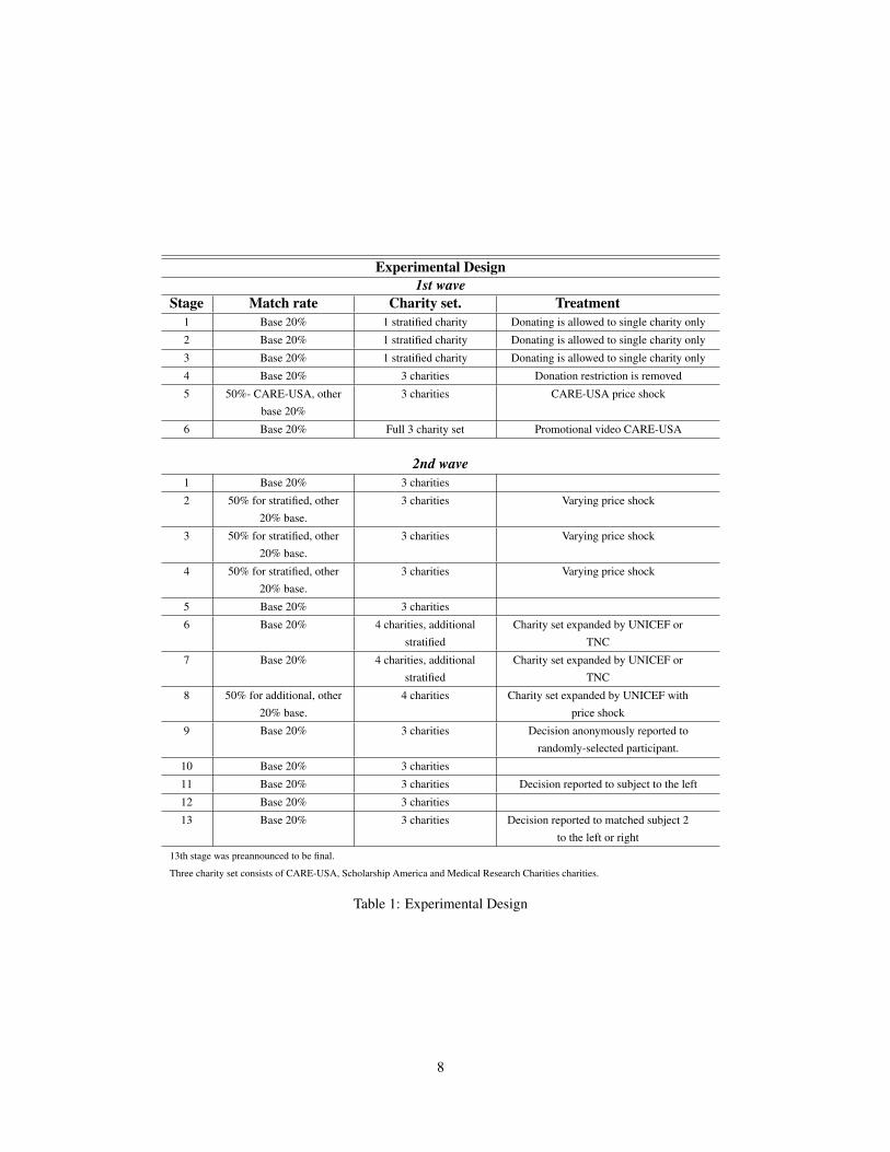
As depicted in table 1, subjects make decisions in six stages, and the outcome of each stage (a payment tothe subject and/or the charities) is realized with equal (1/6) probability. This is explained to subjects in detail,although the precise rules for each stage are not given until the beginning of that stage. This randomized choiceof one stage for payment is standard in economic experiments, and was used in EG’s (2003) charitable givingexperiments, among many others. Under the assumption of expected utility maximization, this setup permitscontrolled within-subject comparisons, without wealth effects of early-round earnings affecting late-roundbehavior (Friedman and Sunder, 1994). Subjects whose preferences meet standard economic assumptions willtreat their decision in one stage as independent of their decision in another stage: they will simply select theoptimal allocation for each stage, since only one will be realized.18 At the end of the experiment the subjectscomplete a survey (on their demographics, charitable giving behavior, and perceptions of the experiment), aredebriefed on the purpose of the experiment, and are paid the amount determined by their choice in therandomlychosen stage, in addition to the initially promised base payment.

In each of the stages, subjects are given an allocation of $10 and the opportunity to donate (out of their$10 allocation) to one or more of the three baseline charities. These donations are matched at (at least) a“baseline” 20% rate in all cases. In stages 1 through 3, only one charity was presented at a time, with thisordering randomized across subjects. In later stages (4-6) I introduce various treatments designed to spur oneof the three causes.19 The treatments are administered in random order where practical; to isolate the effect ofthe promotional information this treatment must be in the final stage.

The “baseline” choice is given in Stage 4 – a subject can donate up to $10 to one or more of three charities,and are informed that the experimenters will add an additional 20% “match” to each of their gifts. There arethree basic kinds of treatments: 1. A limited/expanded choice set: in stages 1-3 participants could only giveto one charity per stage, while in stages 4-6 they could allocate among all three charities (and their ownconsumption) in each stage 2. Price variation: In Stage 5, most subjects were given an increased (50%) 20

matching rate for gifts to the charity CARE, and the usual 20% matching rate for gifts to the other charities3. Information/Propaganda ‘(“video shock”): In Stage 6 most subjects were required to watch a CAREpromotional video. The video is both informative and persuasive. In the terminology of Friedman and Casar(2004) I employ a largely “within-subjects” design, but with some between-subject variation, particularlyin the order the charities are presented and shocked. While the within subjects design reduces variance and“controls for subjects’ personal idiosyncrasies,” the random ordering (for stages 1-3) allows me to control fortime and learning effects. Note that (for both waves) subjects were not informed in advance how many stagestheir would be.

18If subjects are expected-utility maximizers, they will set their decisions to maximize utility in each state of the world. The realizationof a particular stage is a state of the world, and the decision made in that stage will only affect the outcome in that state of the world.Thus, the choice made in one stage does not affect the maximization problem for a choice made in a different stage. A violation of thiswould occur if a subject gains utility from merely the “intention to give” even if the gift is not actually made (e.g., because the stage isnot drawn to be realized).

19In the first wave, second run, I left four subjects out of the higher match rate for Care in stage 4, and 5 subjects were not shown thefilm. In later runs I dropped this control strategy.

20This level was motivated by Meier and Frey (2004), who find that a 50% match increases the propensity to donate, while a 25%match does not. I say “most subjects” because there were several control subjects who were given a repeat of stage 4 conditions insteadof the stage 5 treatment or the stage 6 treatment.

9

4.3. Design: Wave two

Wave two resembles the first wave in many ways. Subjects make donation decisions in a series of stages,one of which is randomly chosen to be realized. Subjects receive an automatic base payment ($5) and aregiven the same endowment in each stage to divide between themselves, and a (varying) set of charities. Otherthan involving a larger endowment, the “baseline” choice, offered in stages one and five, is the same as inwave one, involving the same three charities.

However, there are several important differences. The wave two sessions are longer, involving 13 stages(plus the survey), and the endowment is doubled (now $20) to make each decision roughly as salient (in anexpected value sense) as in wave one. Stages 2-4 offer a “price shock,” a higher (again 50%) match rate,but now offered alternately (with the ordering varied) to each of the three main charities. Stages 6 and 7expand the choice set to a total of four charities, alternately (ordering varied) adding UNICEF and The NatureConservancy. Stage 8 again involves the three “main” charities and UNICEF, but offers a higher (50%) matchrate for gifts to UNICEF. 21 The sequence of stages is depicted in table 1.

5. Experimental Results

22

5.1. Aggregate giving patterns

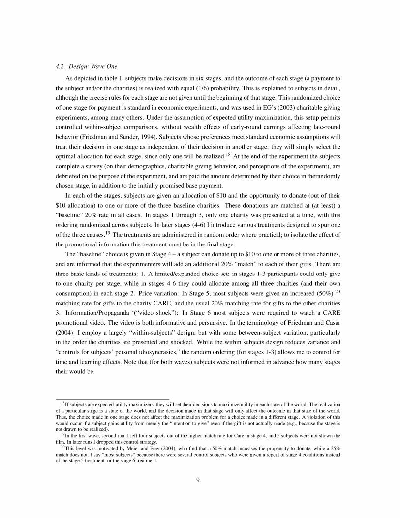
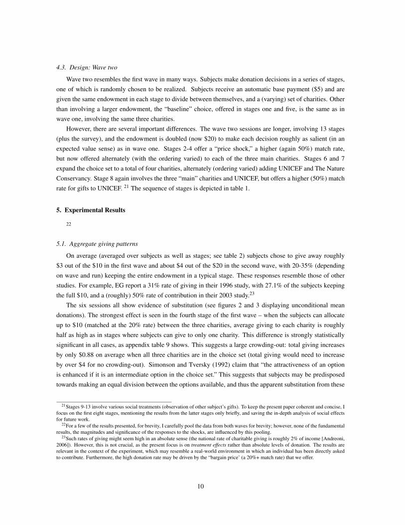
On average (averaged over subjects as well as stages; see table 2) subjects chose to give away roughly$3 out of the $10 in the first wave and about $4 out of the $20 in the second wave, with 20-35% (dependingon wave and run) keeping the entire endowment in a typical stage. These responses resemble those of otherstudies. For example, EG report a 31% rate of giving in their 1996 study, with 27.1% of the subjects keepingthe full $10, and a (roughly) 50% rate of contribution in their 2003 study.23

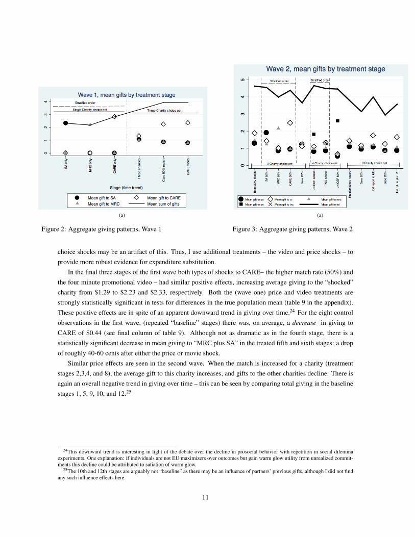
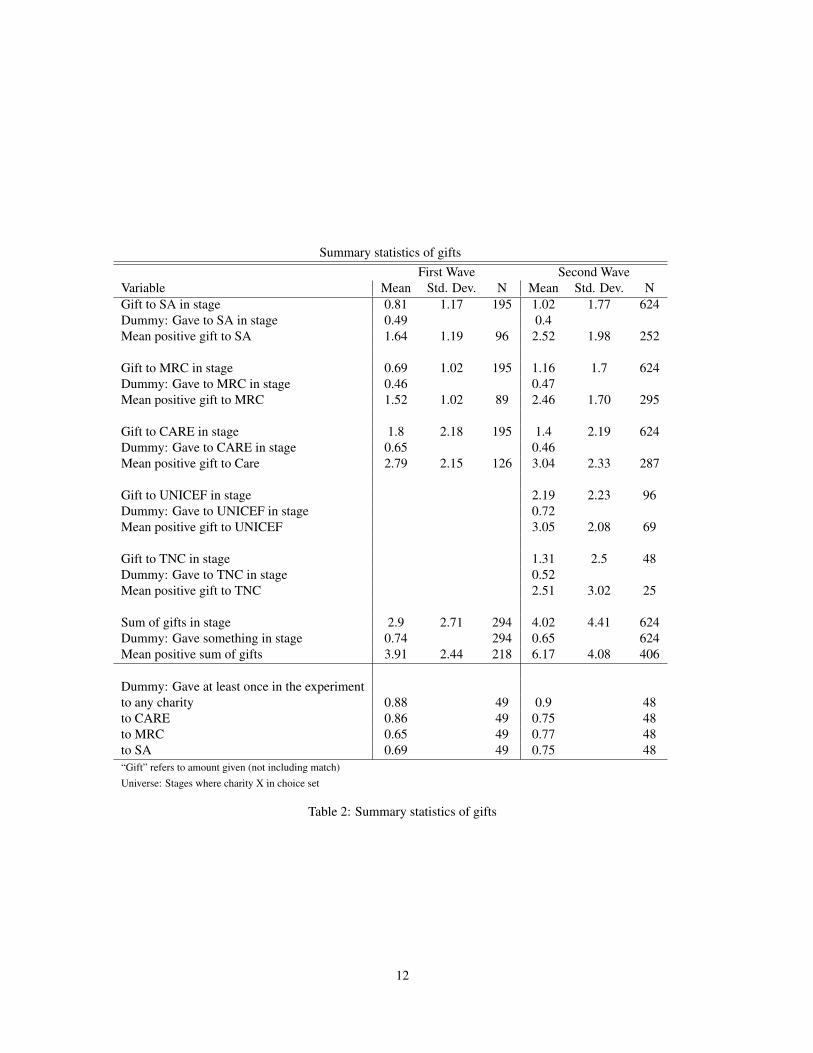
The six sessions all show evidence of substitution (see figures 2 and 3 displaying unconditional meandonations). The strongest effect is seen in the fourth stage of the first wave – when the subjects can allocateup to $10 (matched at the 20% rate) between the three charities, average giving to each charity is roughlyhalf as high as in stages where subjects can give to only one charity. This difference is strongly statisticallysignificant in all cases, as appendix table 9 shows. This suggests a large crowding-out: total giving increasesby only $0.88 on average when all three charities are in the choice set (total giving would need to increaseby over $4 for no crowding-out). Simonson and Tversky (1992) claim that “the attractiveness of an optionis enhanced if it is an intermediate option in the choice set.” This suggests that subjects may be predisposedtowards making an equal division between the options available, and thus the apparent substitution from these

21Stages 9-13 involve various social treatments (observation of other subject’s gifts). To keep the present paper coherent and concise, Ifocus on the first eight stages, mentioning the results from the latter stages only briefly, and saving the in-depth analysis of social effectsfor future work.

22For a few of the results presented, for brevity, I carefully pool the data from both waves for brevity; however, none of the fundamentalresults, the magnitudes and significance of the responses to the shocks, are influenced by this pooling.

23Such rates of giving might seem high in an absolute sense (the national rate of charitable giving is roughly 2% of income [Andreoni,2006]). However, this is not crucial, as the present focus is on treatment effects rather than absolute levels of donation. The results arerelevant in the context of the experiment, which may resemble a real-world environment in which an individual has been directly askedto contribute. Furthermore, the high donation rate may be driven by the “bargain price’ (a 20%+ match rate) that we offer.

10

(a)

Figure 2: Aggregate giving patterns, Wave 1

(a)

Figure 3: Aggregate giving patterns, Wave 2

choice shocks may be an artifact of this. Thus, I use additional treatments – the video and price shocks – toprovide more robust evidence for expenditure substitution.

In the final three stages of the first wave both types of shocks to CARE– the higher match rate (50%) andthe four minute promotional video – had similar positive effects, increasing average giving to the “shocked”charity from $1.29 to $2.23 and $2.33, respectively. Both the (wave one) price and video treatments arestrongly statistically significant in tests for differences in the true population mean (table 9 in the appendix).These positive effects are in spite of an apparent downward trend in giving over time.24 For the eight controlobservations in the first wave, (repeated “baseline” stages) there was, on average, a decrease in giving toCARE of $0.44 (see final column of table 9). Although not as dramatic as in the fourth stage, there is astatistically significant decrease in mean giving to “MRC plus SA” in the treated fifth and sixth stages: a dropof roughly 40-60 cents after either the price or movie shock.

Similar price effects are seen in the second wave. When the match is increased for a charity (treatmentstages 2,3,4, and 8), the average gift to this charity increases, and gifts to the other charities decline. There isagain an overall negative trend in giving over time – this can be seen by comparing total giving in the baselinestages 1, 5, 9, 10, and 12.25

24This downward trend is interesting in light of the debate over the decline in prosocial behavior with repetition in social dilemmaexperiments. One explanation: if individuals are not EU maximizers over outcomes but gain warm glow utility from unrealized commit-ments this decline could be attributed to satiation of warm glow.

25The 10th and 12th stages are arguably not “baseline” as there may be an influence of partners’ previous gifts, although I did not findany such influence effects here.

11

Summary statistics of giftsFirst Wave Second Wave

Variable Mean Std. Dev. N Mean Std. Dev. NGift to SA in stage 0.81 1.17 195 1.02 1.77 624Dummy: Gave to SA in stage 0.49 0.4Mean positive gift to SA 1.64 1.19 96 2.52 1.98 252

Gift to MRC in stage 0.69 1.02 195 1.16 1.7 624Dummy: Gave to MRC in stage 0.46 0.47Mean positive gift to MRC 1.52 1.02 89 2.46 1.70 295

Gift to CARE in stage 1.8 2.18 195 1.4 2.19 624Dummy: Gave to CARE in stage 0.65 0.46Mean positive gift to Care 2.79 2.15 126 3.04 2.33 287

Gift to UNICEF in stage 2.19 2.23 96Dummy: Gave to UNICEF in stage 0.72Mean positive gift to UNICEF 3.05 2.08 69

Gift to TNC in stage 1.31 2.5 48Dummy: Gave to TNC in stage 0.52Mean positive gift to TNC 2.51 3.02 25

Sum of gifts in stage 2.9 2.71 294 4.02 4.41 624Dummy: Gave something in stage 0.74 294 0.65 624Mean positive sum of gifts 3.91 2.44 218 6.17 4.08 406

Dummy: Gave at least once in the experimentto any charity 0.88 49 0.9 48to CARE 0.86 49 0.75 48to MRC 0.65 49 0.77 48to SA 0.69 49 0.75 48“Gift” refers to amount given (not including match)Universe: Stages where charity X in choice set

Table 2: Summary statistics of gifts

12

5.2. Individual-level Analysis: Substitution

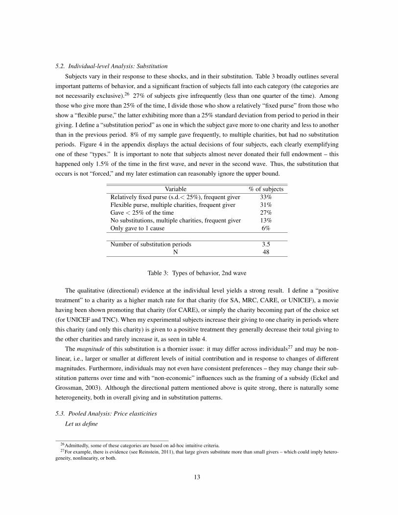
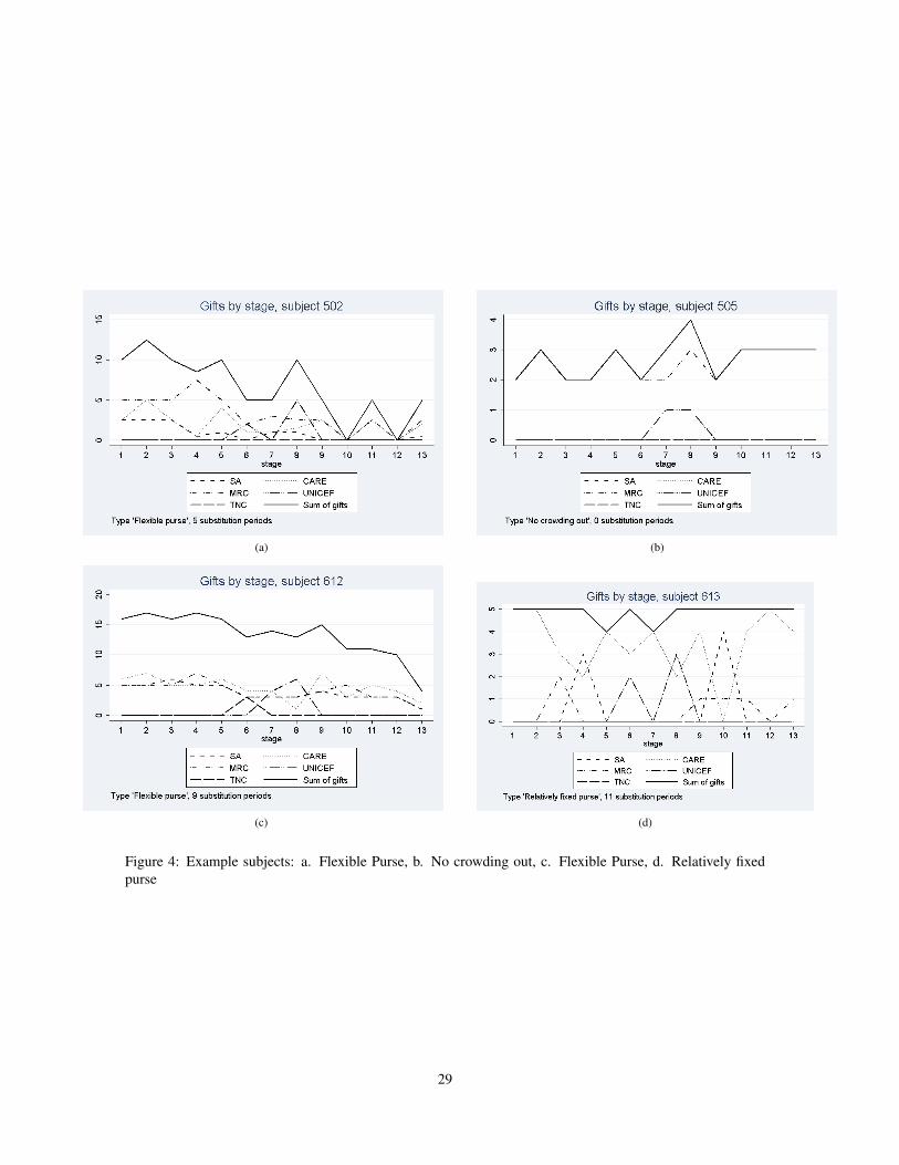
Subjects vary in their response to these shocks, and in their substitution. Table 3 broadly outlines severalimportant patterns of behavior, and a significant fraction of subjects fall into each category (the categories arenot necessarily exclusive).26 27% of subjects give infrequently (less than one quarter of the time). Amongthose who give more than 25% of the time, I divide those who show a relatively “fixed purse” from those whoshow a “flexible purse,” the latter exhibiting more than a 25% standard deviation from period to period in theirgiving. I define a “substitution period” as one in which the subject gave more to one charity and less to anotherthan in the previous period. 8% of my sample gave frequently, to multiple charities, but had no substitutionperiods. Figure 4 in the appendix displays the actual decisions of four subjects, each clearly exemplifyingone of these “types.” It is important to note that subjects almost never donated their full endowment – thishappened only 1.5% of the time in the first wave, and never in the second wave. Thus, the substitution thatoccurs is not “forced,” and my later estimation can reasonably ignore the upper bound.

Variable % of subjectsRelatively fixed purse (s.d.< 25%), frequent giver 33%Flexible purse, multiple charities, frequent giver 31%Gave < 25% of the time 27%No substitutions, multiple charities, frequent giver 13%Only gave to 1 cause 6%

Number of substitution periods 3.5N 48

Table 3: Types of behavior, 2nd wave

The qualitative (directional) evidence at the individual level yields a strong result. I define a “positivetreatment” to a charity as a higher match rate for that charity (for SA, MRC, CARE, or UNICEF), a moviehaving been shown promoting that charity (for CARE), or simply the charity becoming part of the choice set(for UNICEF and TNC). When my experimental subjects increase their giving to one charity in periods wherethis charity (and only this charity) is given to a positive treatment they generally decrease their total giving tothe other charities and rarely increase it, as seen in table 4.

The magnitude of this substitution is a thornier issue: it may differ across individuals27 and may be non-linear, i.e., larger or smaller at different levels of initial contribution and in response to changes of differentmagnitudes. Furthermore, individuals may not even have consistent preferences – they may change their sub-stitution patterns over time and with “non-economic” influences such as the framing of a subsidy (Eckel andGrossman, 2003). Although the directional pattern mentioned above is quite strong, there is naturally someheterogeneity, both in overall giving and in substitution patterns.

5.3. Pooled Analysis: Price elasticities

Let us define

26Admittedly, some of these categories are based on ad-hoc intuitive criteria.27For example, there is evidence (see Reinstein, 2011), that large givers substitute more than small givers – which could imply hetero-

geneity, nonlinearity, or both.

13

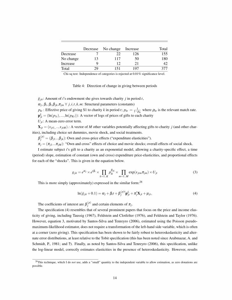
Decrease No change Increase TotalDecrease 7 22 126 155No change 13 117 50 180Increase 9 12 21 42Total 29 151 197 377

Chi-sq test: Independence of categories is rejected at 0.01% significance level.

Table 4: Direction of change in giving between periods

g̈ jit : Amount of i’s endowment she gives towards charity j in period t,a j, bi, bt ,b jk,p jm 8 j, i, t,k,m: Structural parameters (constants)pkt : Effective price of giving $1 to charity k in period t; pkt = 1

1�rktwhere rkt is the relevant match rate.

p

Ljt = (ln(p1t), ..., ln(pKt)): A vector of logs of prices of gifts to each charity

Ujt : A mean-zero error term.X jt = (x jt1,...,x jtM).: A vector of M other variables potentially affecting gifts to charity j (and other char-

ities), including choice set dummies, movie shock, and social treatments.b (p)

j = (b j1...b jk): Own and cross-price effects (“expenditure elasticities”).p j = (p j1...p jM): “Own and cross” effects of choice and movie shocks; overall effects of social shock.I estimate subject i’s gift to a charity as an exponential model, allowing a charity-specific effect, a time

(period) slope, estimation of constant (own and cross) expenditure price-elasticities, and proportional effectsfor each of the “shocks”. This is given in the equation below.

g jit = ea j ⇥ etbt ⇥ ’k=1..K

pb jkkt ⇥ ’

m=1..Mexp(x jtmp jm)⇥Ujt (3)

This is more simply (approximately) expressed in the similar form:28

ln(g̈ jit +0.1) = a j +bt t +b (p)0j p

Ljt +p 0

jX jt +µ jt , (4)

The coefficients of interest are b (p)j and certain elements of p j.

The specification (4) resembles that of several prominent papers that focus on the price and income elas-ticity of giving, including Taussig (1967), Feldstein and Clotfelter (1976), and Feldstein and Taylor (1976).However, equation 3, motivated by Santos-Silva and Tenreyro (2006), estimated using the Poisson pseudo-maximum-likelihood estimator, does not require a transformation of the left-hand side variable, which is oftenat a corner (zero giving). This specification has been shown to be fairly robust to heteroskedasticity and alter-nate error distributions, at least relative to the Tobit specification (this has been noted since Arabmazar, A. andSchmidt, P., 1981; and ?). Finally, as noted by Santos-Silva and Tenreyro (2006), this specification, unlikethe log-linear model, correctly estimates elasticities in the presence of heteroskedasticity. However, results

28This technique, which I do not use, adds a ”small” quantity to the independent variable to allow estimation, as zero donations arepossible.

14

(available by request) from the log-linear model, adding $0.10 to all contribution variables, do not differ sub-stantially, nor do results from the Tobit or “Heckit” models. Given the correct functional form specification,standard identification conditions should hold here, since the regressors vary exogenously by design.

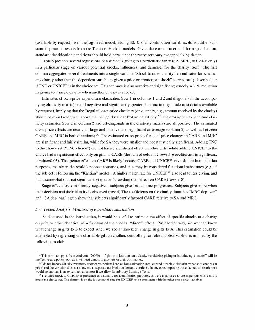
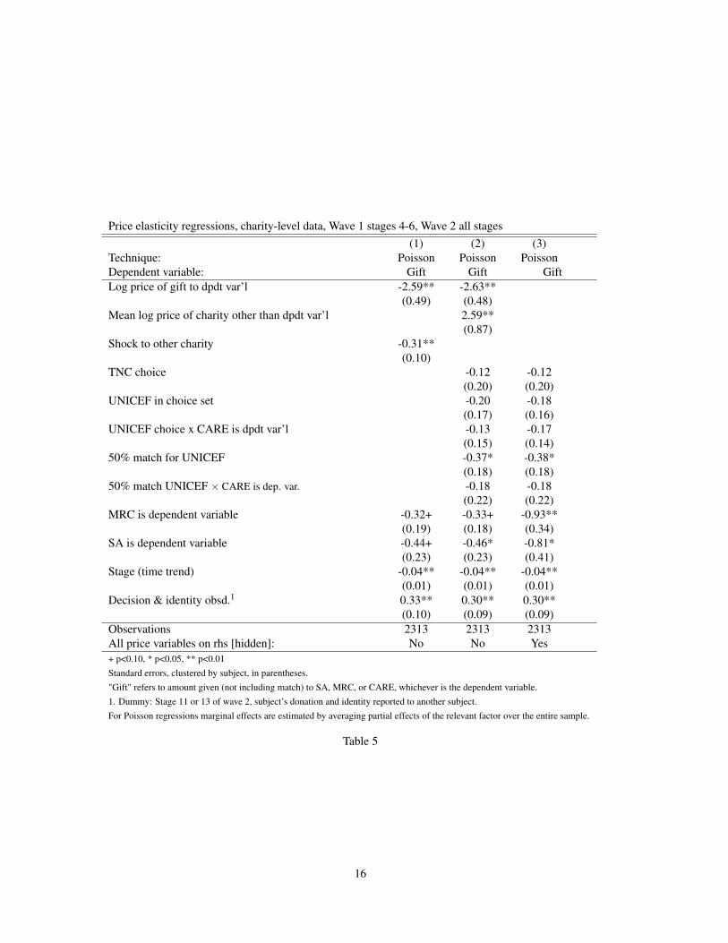
Table 5 presents several regressions of a subject’s giving to a particular charity (SA, MRC, or CARE only)in a particular stage on various potential shocks, influences, and dummies for the charity itself. The firstcolumn aggregates several treatments into a single variable “Shock to other charity” an indicator for whetherany charity other than the dependent variable is given a price or promotion “shock” as previously described, orif TNC or UNICEF is in the choice set. This estimate is also negative and significant; crudely, a 31% reductionin giving to a single charity when another charity is shocked.

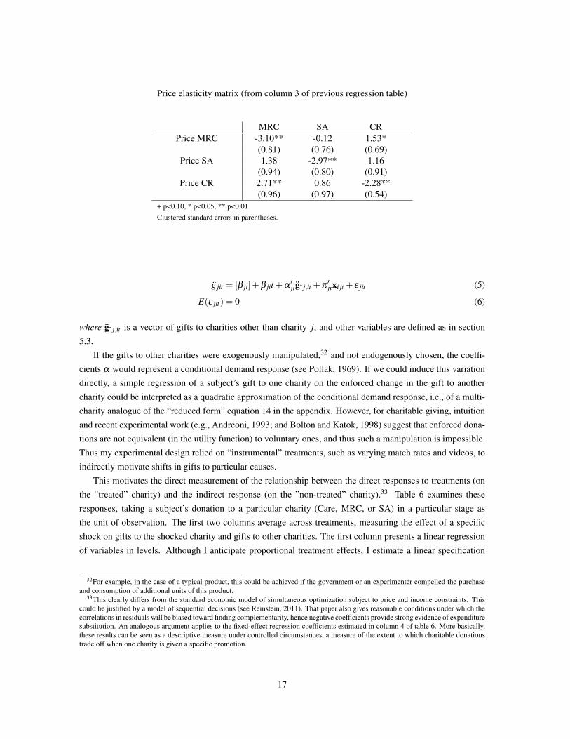
Estimates of own-price expenditure elasticities (row 1 in columns 1 and 2 and diagonals in the accompa-nying elasticity matrix) are all negative and significantly greater than one in magnitude (test details availableby request), implying that the “regular” own-price elasticity (on quantity, e.g., amount received by the charity)should be even larger, well above the the “gold standard”of unit elasticity.29 The cross-price expenditure elas-ticity estimates (row 2 in column 2 and off-diagonals in the elasticity matrix) are all positive. The estimatedcross-price effects are nearly all large and positive, and significant on average (column 2) as well as betweenCARE and MRC in both directions).30 The estimated cross-price effects of price changes in CARE and MRCare significant and fairly similar, while for SA they were smaller and not statistically significant. Adding TNCto the choice set (“TNC choice”) did not have a significant effect on other gifts, while adding UNICEF to thechoice had a significant effect only on gifts to CARE (the sum of column 2 rows 5-6 coefficients is significant,p-value=0.03). The greater effect on CARE is likely because CARE and UNICEF serve similar humanitarianpurposes, mainly in the world’s poorest countries, and thus may be considered functional substitutes (e.g., ifthe subject is following the “Kantian” model). A higher match rate for UNICEF31 also lead to less giving, andhad a somewhat (but not significantly) greater “crowding out” effect on CARE (rows 7-8).

Stage effects are consistently negative – subjects give less as time progresses. Subjects give more whentheir decision and their identity is observed (row 4).The coefficients on the charity dummies “MRC dep. var.”and “SA dep. var.” again show that subjects significantly favored CARE relative to SA and MRC.

5.4. Pooled Analysis: Measures of expenditure substitution

As discussed in the introduction, it would be useful to estimate the effect of specific shocks to a charityon gifts to other charities, as a function of the shocks’ “direct” effect. Put another way, we want to knowwhat change in gifts to B to expect when we see a “shocked” change in gifts to A. This estimation could beattempted by regressing one charitable gift on another, controlling for relevant observables, as implied by thefollowing model:

29This terminology is from Andreoni (2006b) – if giving is less than unit-elastic, subsidizing giving or introducing a “match” will beineffective as a policy tool, as it will lead donors to give less of their own money.

30I do not impose Slutsky symmetry or other restrictions here, as I am estimating gross expenditure elasticities (in response to changes inprice) and the variation does not allow me to separate out Hicksian demand elasticies. In any case, imposing these theoretical restrictionswould be dubious in an experimental context if we allow for arbitrary framing effects.

31The price shock to UNICEF is presented as a dummy for identification purposes, as there is no price to use in periods where this isnot in the choice set. The dummy is on the lower match rate for UNICEF, to be consistent with the other cross-price variables.

15

Price elasticity regressions, charity-level data, Wave 1 stages 4-6, Wave 2 all stages(1) (2) (3)

Technique: Poisson Poisson PoissonDependent variable: Gift Gift GiftLog price of gift to dpdt var’l -2.59** -2.63**

(0.49) (0.48)Mean log price of charity other than dpdt var’l 2.59**

(0.87)Shock to other charity -0.31**

(0.10)TNC choice -0.12 -0.12

(0.20) (0.20)UNICEF in choice set -0.20 -0.18

(0.17) (0.16)UNICEF choice x CARE is dpdt var’l -0.13 -0.17

(0.15) (0.14)50% match for UNICEF -0.37* -0.38*

(0.18) (0.18)50% match UNICEF ⇥ CARE is dep. var. -0.18 -0.18

(0.22) (0.22)MRC is dependent variable -0.32+ -0.33+ -0.93**

(0.19) (0.18) (0.34)SA is dependent variable -0.44+ -0.46* -0.81*

(0.23) (0.23) (0.41)Stage (time trend) -0.04** -0.04** -0.04**

(0.01) (0.01) (0.01)Decision & identity obsd.1 0.33** 0.30** 0.30**

(0.10) (0.09) (0.09)Observations 2313 2313 2313All price variables on rhs [hidden]: No No Yes+ p<0.10, * p<0.05, ** p<0.01Standard errors, clustered by subject, in parentheses."Gift" refers to amount given (not including match) to SA, MRC, or CARE, whichever is the dependent variable.1. Dummy: Stage 11 or 13 of wave 2, subject’s donation and identity reported to another subject.For Poisson regressions marginal effects are estimated by averaging partial effects of the relevant factor over the entire sample.

Table 5

16

Price elasticity matrix (from column 3 of previous regression table)

MRC SA CRPrice MRC -3.10** -0.12 1.53*

(0.81) (0.76) (0.69)Price SA 1.38 -2.97** 1.16

(0.94) (0.80) (0.91)Price CR 2.71** 0.86 -2.28**

(0.96) (0.97) (0.54)+ p<0.10, * p<0.05, ** p<0.01Clustered standard errors in parentheses.

g̈ jit = [b ji]+b jit +a 0ji ¨g˜ j,it +p 0

jixi jt + e jit (5)

E(e jit) = 0 (6)

where ¨

g˜ j,it is a vector of gifts to charities other than charity j, and other variables are defined as in section5.3.

If the gifts to other charities were exogenously manipulated,32 and not endogenously chosen, the coeffi-cients a would represent a conditional demand response (see Pollak, 1969). If we could induce this variationdirectly, a simple regression of a subject’s gift to one charity on the enforced change in the gift to anothercharity could be interpreted as a quadratic approximation of the conditional demand response, i.e., of a multi-charity analogue of the “reduced form” equation 14 in the appendix. However, for charitable giving, intuitionand recent experimental work (e.g., Andreoni, 1993; and Bolton and Katok, 1998) suggest that enforced dona-tions are not equivalent (in the utility function) to voluntary ones, and thus such a manipulation is impossible.Thus my experimental design relied on “instrumental” treatments, such as varying match rates and videos, toindirectly motivate shifts in gifts to particular causes.

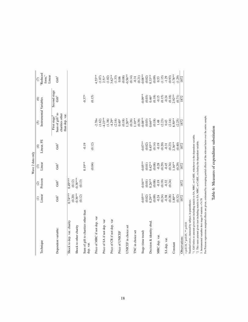
This motivates the direct measurement of the relationship between the direct responses to treatments (onthe “treated” charity) and the indirect response (on the ”non-treated” charity).33 Table 6 examines theseresponses, taking a subject’s donation to a particular charity (Care, MRC, or SA) in a particular stage asthe unit of observation. The first two columns average across treatments, measuring the effect of a specificshock on gifts to the shocked charity and gifts to other charities. The first column presents a linear regressionof variables in levels. Although I anticipate proportional treatment effects, I estimate a linear specification

32For example, in the case of a typical product, this could be achieved if the government or an experimenter compelled the purchaseand consumption of additional units of this product.

33This clearly differs from the standard economic model of simultaneous optimization subject to price and income constraints. Thiscould be justified by a model of sequential decisions (see Reinstein, 2011). That paper also gives reasonable conditions under which thecorrelations in residuals will be biased toward finding complementarity, hence negative coefficients provide strong evidence of expendituresubstitution. An analogous argument applies to the fixed-effect regression coefficients estimated in column 4 of table 6. More basically,these results can be seen as a descriptive measure under controlled circumstances, a measure of the extent to which charitable donationstrade off when one charity is given a specific promotion.

17

Wav

e2

data

only

(1)

(2)

(3)

(4)

(5)

(6)

(7)

Tech

niqu

eLi

near

Pois

son

Line

arLi

near

,FE

Inst

rum

enta

lVar

iabl

es“R

educ

edfo

rm,”

Line

arFi

rsts

tage

3Se

cond

stag

eD

epen

dent

varia

ble:

Gift

1G

ift1

Gift

1G

ift1

Sum

ofgi

ft2to

char

ities

othe

rth

ande

p.va

r.

Gift

1G

ift1

Shoc

kto

dep.

var.

char

ity0.

74**

*0.

49**

*(0

.20)

(0.1

2)Sh

ock

toot

herc

harit

y-0

.36*

*-0

.38*

**(0

.12)

(0.1

3)Su

mof

gift

toch

ariti

esot

hert

han

dep.

var.

0.19

**-0

.19

-0.3

7*

(0.0

4)(0

.12)

(0.1

5)Pr

ice

ofM

RC

ifno

tdep

.var

-2.7

8+4.

55**

(1.6

2)(1

.07)

Pric

eof

SAif

notd

ep.v

ar-4

.23*

*2.

51*

(1.3

8)(1

.02)

Pric

eof

CR

ifno

tdep

.var

-4.2

9*3.

62**

(2.1

4)(1

.33)

Pric

eof

UN

ICEF

0.40

*0.

06(0

.18)

(0.0

8)U

NIC

EFin

choi

cese

t1.

28**

-0.5

6**

(0.2

6)(0

.14)

TNC

inch

oice

set

1.10

**-0

.31

(0.3

9)(0

.21)

Stag

e(ti

me

trend

)-0

.05*

*-0

.04*

*-0

.05*

*-0

.07*

*-0

.08*

*-0

.09*

*-0

.08*

*(0

.02)

(0.0

1)(0

.01)

(0.0

2)(0

.03)

(0.0

3)(0

.02)

Dec

isio

n&

iden

tity

obsd

.0.

29**

0.26

**0.

42**

0.45

**0.

64**

0.46

*0.

33**

(0.0

9)(0

.08)

(0.0

8)(0

.14)

(0.1

8)(0

.18)

(0.0

9)M

RC

dep.

var.

-0.2

4-0

.19

-0.2

8-0

.19

1.48

-0.1

50.

53(0

.24)

(0.1

9)(0

.29)

(0.2

0)(2

.23)

(0.1

5)(1

.15)

SAde

p.va

r.-0

.38

-0.3

2-0

.45

-0.3

10.

43-0

.24

-1.2

9(0

.28)

(0.2

4)(0

.34)

(0.2

3)(2

.14)

(0.1

8)(0

.93)

Con

stan

t1.

80**

1.16

**2.

36**

8.50

**2.

92**

-3.7

8**

(0.3

2)(0

.29)

(0.4

0)(2

.25)

(0.7

1)(1

.29)

Obs

erva

tions

1872

1872

1872

1872

1872

1872

1872

+p<

0.10

,*p<

0.05

,**

p<0.

01St

anda

rder

rors

,clu

ster

edby

subj

ect,

inpa

rent

hese

s."1

.Gift

"ref

ers

toam

ount

give

n(n

otin

clud

ing

mat

ch)t

oSA

,MR

C,o

rCA

RE,

whi

chev

eris

the

depe

nden

tvar

iabl

e."2

.Thi

ssu

ms

amou

ntgi

ven

(not

incl

udin

gm

atch

)to

SA,M

RC

,orC

AR

E,ex

clud

ing

the

depe

nden

tvar

iabl

e.3.

Inst

rum

enta

lvar

iabl

esfir

stst

age

F-st

atis

tic=7

4.70

ForP

oiss

onre

gres

sion

sm

argi

nale

ffec

tsar

egi

ven,

estim

ated

byav

erag

ing

parti

alef

fect

sof

the

rele

vant

fact

orov

erth

een

tire

sam

ple.

Tabl

e6:

Mea

sure

sof

expe

nditu

resu

bstit

utio

n

18

here both to give an easy intuitive interpretation, and more importantly, because I want to compare the twocoefficients (own and other shock) to focus on a linear “expenditure substitution” response (see equation5), to be able to identify the ’rate’ (zero, full, partial) at which one contribution crowds out another. Thesecond column gives the exponential specification as in table 5, to demonstrate the robustness of the results tovariations in functional form assumptions. The estimates are qualitatively the same and close in magnitude.

As anticipated, in both columns 1 and 2, the shocks have significant positive direct effects as well assignificant negative indirect effects. The ratio of coefficients on these dummy variables in column 1, approx-imately �0.49, provides a crude measure of the “crowding out” effect examined in the later columns. ForColumn 2 the estimated ratio of average marginal effects is almost �0.78. In nonlinear (Wald) tests, the ratiois significantly different from zero for both columns 1 and 2.

Columns 3 and 4 directly measure the relationship between gifts to one charity and gifts to another. Inlight of the above discussion, I present these results cautiously; the “responses” estimated above might be seenas descriptive, rather than causal. They are intended to reflect the relationship between changes in donations todistinct charities when one charity is a “specific” shock. Still, even with exogenous treatments, a simple OLSestimation of (e.g) equation 5 of one charitable gift on another may still not be a consistent measure of thisrelationship. In particular, it is not clear that the identification condition E(e jit ⇥ e˜ jit) = 0 8 j, ˜ j will hold.In fact, the coefficient goes from 0.19 to -0.19 when we include a subject-fixed effect, strongly suggesting anindividual-specific unobservable “predilection to donate” term. However, even controlling for this, we cannotrule out the possibility that a subject’s overall generosity may vary in specific periods for other reasons,biasing the estimates of conditional demand effects in a positive direction (towards finding complementarity).However, an instrumental variables approach essentially isolates only the component of (changes in) charitablegiving to a cause that is explained by the exogenous treatment(s) specific to that charity, and measures howthe other donations respond to this “exogenously shifted” change. Thus, an IV measure should not be affectedby a random fluctuation, from period to period, in overall generosity or in the subjects subjective earningstarget.34

The instrumental variable results support the claim that this time-variant error term tends to be positivelycorrelated across charities. The result reported in row 3 of column 6 is even more strongly negative thanthe “conditional correlation” fixed-effects regressions reported in column 4. The IV results suggest a showa “crowding out” of �.37, slightly below the ratio of coefficients in column 1. This IV coefficient can beinterpreted as measuring the conditional demand response of gifts to charity ‘B’ of variation in gifts to charity‘A’, only insofar as the variation in giving to ‘A’ is driven by the exogenous instruments (treatments). Forcompleteness and clarity, I give the first stage results in column 5, noting that the first stage is very strong(F=74.70), and I give the “reduced form” results in column 7.

6. Robustness Checks

6.1. Internal validity issues

Each stage in the experiment is realized with equal probability, and only one stage is realized. Thus, theclassical expected-utility maximizer should treat each stage independently. However, from a psychological

34See Loomes (2005) for a related discussion of the experimental “error term”.

19

perspective, previous stages may cast a shadow on future behavior. In particular, one might worry that offeringa higher match rate and then taking it away, as in wave two stage five, would discourage later giving. However,there is no strong evidence of a particular discouragement effect in this stage, as seen in appendix table 13.The estimated coefficient on the stage 5 dummy is negative but small and statistically insignificant, and theown-price and cross-price elasticities remain large and significant in the presence of this control.

A common criticism of laboratory experiments is that the monetary incentives and experimental treatmentsdo not dominate the “noise”, and that the amounts of money at stake are too small to be taken seriously. Insuch a case, if we increase the stake enough, the incentives to maximize should increase, and the subjects’decisions should become more responsive to the treatments. In the present context, the results are broadlysimilar between the first and second waves, each with different stake sizes. This can be seen in figures 2 and3, as well as in table 2 and 13.35

I note that most subjects take more than the minimum time to enter their choices (figure 5 in the appendix),suggesting that the incentives are at least somewhat salient. Still, as for most such experiments measuring”homegrown values,” we can not rule out the possibility that behavior would differ if much larger amountswere at stake.

Credibility and comprehension is always an issue in laboratory experiments. Table 8 in the appendixshows that the vast majority of the subjects claim that they understood the experiment and were confident inits truthfulness. A smaller majority had confidence in the charities themselves.

6.2. External Generalizability

While Friedman and Sunder (1994) claim that the skeptic “has the burden of stating what is different aboutthe outside world that might change the result observed in the laboratory,” other authors, such as Levitt andList (Levitt and List), are more skeptical. Although Benz and Meier 2006 offer evidence that experimentalbehavior in charitable giving is correlated to field behavior, there is still a lack of evidence on this question. Ithus consider several possible limits to the generalizability of my findings.

Harrison (2002) notes that “lab responses may be censored by field opportunities.” A subject may under-report her valuation if a good is cheaper in the field. I address this in part with the baseline 20% matchrate, which (particularly for those who do not itemize deductions on their taxes) should make gifts in thelaboratory a bargain. If a subject can re-sell a good, she may over-report her true valuation. In the presentexperiment, a subject might donate in the laboratory and in turn reduce her giving in the field. I differentiatethe results in table 10 (in the appendix) by including an interaction term (column 1) and then running aseparate regression (column 2), for those who claim to have donated previously,36 to detect whether suchintertemporal substitution may be occurring. In the first column, although the interaction terms suggestsgreater responsiveness to prices, perhaps driven by greater intertemporal substitution, these terms are notsignificant. The second column’s regression shows similar price effects for the “non-outside-givers” as for the“outside givers” suggesting that intertemporal substitution is not driving my main results.

35Table 13 (in the appendix) differentiates by wave and run, estimating a basic measure of the extent to which an individual substi-tutes one contribution for another, allowing for individual fixed-effects. These regressions also model parameter heterogeneity usingStata’s “xtrc” to efficiently estimate average coefficients and their standard errors under the assumption of normally distributed errors andconditional homoskedasticity. However, standard fixed-effect regressions for each column (available by request) yield similar coefficients.

36For each of the five charities, the subjects were asked the amount they previously gave to charities “similar to” the ones listed in thepast year. The “Gave outside dummy” indicates whether the subject reported giving a positive amount for any of these five questions.

20

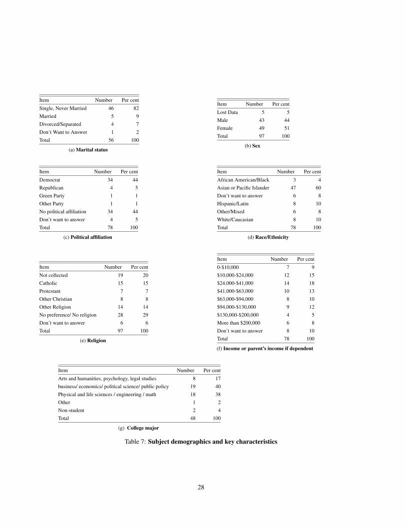
As the demographics (tables 7a-7g in the appendix) show, my sample is not representative of the Americanpopulation at large, nor of the population of charitable donors. I employ the typical “convenience sample” ofstudents (and some university staff), paid volunteers for such an experiment, young, educated, and living in aliberal academic setting. While this may not be a problem for testing a theory of universal behavior, it is well-known that there are wide differences in charitable giving behavior among socioeconomic groups (Harrisonand List, 2004). While I observe some heterogeneity in substitution patterns, as reported in section 5.2 (andI explicitly model random parameter heterogeneity in appendix table 12), there are no clear and significantpatterns along observable socioeconomic lines. Table 11 in the appendix shows treatment coefficients that arefairly similar across the various groups in my study, looking across sex, ethnicity, and religious identification.37

Note that I do not observe meaningful variation in categories such as education, region, or age. Future workshould expand the sample along these dimensions.

My estimates focus on how a subject’s behavior responds to the treatments presented, allowing me tocontrol for substantial between-subject heterogeneity. However as Camerer 1995 notes, “presenting severalstimuli to a single subject could conceivably induce her to behave more consistently than she would if shesaw the stimuli one at a time.” Other work (Huber et al., 1982; Simonson and Tversky 1992) also notes thatindividuals are particularly sensitive to relative changes and to contrasts between several choices that are pre-sented simultaneously or within a short interval. However, it is not clear that isolated decisions (as in a purelybetween-subject design) would better reflect the relevant field environments than the ones presented in myexperiment. In many real world charitable giving environments individuals are faced with several proximatesolicitations and donation decisions, and can closely compare charities. For example, many countries andworkplaces promote payroll giving programs (such as the UK’s “Give as You Earn” and the “Combined Fed-eral Campaign” in the USA), presenting employees with a large catalogue of charities from which they canchoose to make a pre-tax donation.

Overall, my results provide suggestive evidence that substitution will be relevant to some real-world en-vironments, and that this merits future study. Still, it is unlikely that the estimated magnitudes of price andsubstitution effects are relevant for policy simulation. As noted, these responses are likely to be heterogeneousacross individuals, across time, and across modes of giving, may be sensitive to the proximity and framingof the choices, and to the magnitude of the stakes. While previous work has found some connections be-tween laboratory and field behavior, other work has found variation according to the nature and magnitude ofthe (laboratory) earnings, and the typical “convenience sample” of self-selected university students has beenfound to behave differently from other groups in important ways (surveyed in Levitt and List).

7. Conclusion

This series of experiments offers some of the first evidence on how people give to multiple charities inthe lab. The direct effects of treatments were strong and for the choice and video shocks, in the predicteddirection (for the match shock the standard theoretical prediction was ambiguous). Most shocks are effective:people give more to a charity when its match rate was higher, when the decision was observed, when they

37While those who do not report a high income (column 4) are somewhat less price sensitive then other subjects and show lessexpenditure substitution, the signs are the same in both cases, and these differences are not significant (results available by request). Still,this weakly suggests that substitution behavior might vary by income.

21

were motivated by a video, and when there were fewer other charities in the choice set. Several of these directeffects are interesting in themselves; as mentioned before, the gifts are own-price elastic with regard to matchrates, contrasting with some previous literature (see, e.g., earlier footnote on EG’s results).

The results demonstrate that “expenditure substitution” among charities can be seen in a laboratory set-ting. I find large own-price and large positive cross-price expenditure elasticities – these charities are grosssubstitutes in the conventional sense. The substitution is stronger where the charities serve similar purposes,such as UNICEF and CARE.

These estimates obscure a great deal of heterogeneity– subjects vary greatly in their substitution patterns,as seen in section 5.2 and in appendix tables 12 and 13. In broad terms, my results support Reinstein (2011),which uses observational panel data (the PSID/COPPS) and finds expenditure substitution, particularly be-tween giving to health and giving to either basic needs or educational charities.38 These papers motivatefuture investigation; in particular, field experiments may also prove a fruitful way to combine the strengths ofthe laboratory and happenstance data. For example, a design (in the mold of Frey and Meier, 2004; or Rasuland Huck, 2010) taking advantage of differential employer-provided incentives to donate to specific charitiescould allow a well-identified direct estimation of own and cross-price elasticities for a relevant population overa relevant domain of behavior.

References

Alpizar, F., F. Carlsson, and O. Johansson-Stenman (2008). Anonymity, reciprocity, and conformity: Evidencefrom voluntary contributions to a national park in Costa Rica. Journal of Public Economics 92(5-6), 1047–1060.

Andreoni, J. (1990). Impure altruism and donations to public goods: A theory of warm-glow giving. TheEconomic Journal 100, 464–477.

Andreoni, J. (1993, December). An experimental test of the public-goods crowding-out hypothesis. TheAmerican Economic Review 83(5), 1317–1327.

Andreoni, J. (2006a). Philanthropy, handbook of giving, reciprocity and altruism, sc. kolm and j. mercierythier, eds.

Andreoni, J. (2006b). Philanthropy, handbook of giving, reciprocity and altruism, sc. kolm and j. mercierythier, eds. Amsterdam, North Holland 1201, 1269.

Andreoni, J., W. Gale, and J. Scholz (1996). Charitable Contributions of Time and Money. University ofWisconsin–Madison Working Paper.

Andreoni, J. and J. Miller (2002, mar). Giving according to garp: An experimental test of the consistency ofpreferences for altruism. Econometrica 70(2), 737–753.

Becker, G. S. (1974, nov). A theory of social interactions. The Journal of Political Economy 82(6), 1063–1093.

38Expenditure substitution was present specifically for larger donors, those who gave more than $1000 in a year previous to the dataanalyzed; the subjects in the present experiment are unlikely to have ever contributed this much.

22

Bekkers, R. and P. Wiepking (2008). Generosity and Philanthropy: A Literature Review. Working paper..

Benabou, R. and J. Tirole (2003). Intrinsic and Extrinsic Motivation. Review of Economic Studies 70(3),489–520.

Benz, M. and S. Meier (2006). Do People Behave in Experiments as in the Field?–Evidence from Donations.Institute for Empirical Research in Economics, University of Zurich, manuscript. Good connection betweenlab and field charitable giving.

Bilodeau, M. and A. Slivinski (1997). Rival charities. Journal of Public Economics 66(3), 449–467.

Bolton, G. and E. Katok (1998). An experimental test of the crowding out hypothesis: The nature of beneficentbehavior. Journal of Economic Behavior and Organization 37(3), 315–331.

Borgloh, S. (2009). Have You Paid Your Dues? On the Impact of the German Church Tax on Private CharitableContributions. Working Paper, Centre for European Economic Research.

Camerer, C. (1995). Individual decision making. The handbook of experimental economics 3, 587–704.

Carman, K. (2003). Social influences and the private provision of public goods: Evidence from charitablecontributions in the workplace. Manuscript, Stanford University.

Chua, V. and C. Ming Wong (2003). The role of united charities in fundraising: The case of singapore. Annalsof Public and Cooperative Economics 74(3), 433–464.

Duncan, B. (2004). A theory of impact philanthropy. Journal of Public Economics 88(9-10), 2159–2180.

Eckel, C. and P. Grossman (1996). Altruism in anonymous dictator games. Games and Economic Behav-ior 16(2), 181–191.

Eckel, C. and P. Grossman (2003). Rebate versus matching: Does how we subsidize charitable contributionsmatter? Journal of Public Economics 87(3-4), 681–701.

Eckel, C. and P. Grossman (2006). Do donors care about subsidy type? an experimental study. Research inexperimental economics 11, 163–182.

Eckel, Catherine C. and Grossman, Philip J. (1998, may). Are women less selfish than men?: Evidence fromdictator experiments. The Economic Journal 108(448), 726–735.

Falk, A. (2004). Charitable giving as a gift exchange: Evidence from a field experiment.

Feldstein, M. and C. Clotfelter (1976). Tax incentives and charitable organizations in the united states. Journalof Public Economics 5(1-2), 1–26.

Feldstein, M. and A. Taylor (1976, nov). The income tax and charitable contributions. Econometrica 44(6),1201–1222.

Fisman, R., S. Kariv, and D. Markovits (2005). Individual preferences for giving. Yale Law & EconomicsResearch Paper.

23

Frey, B. and S. Meier (2004). Pro-social behavior in a natural setting. Journal of Economic Behavior andOrganization 54(1), 65–88.

Frey and Meier (2004). Social comparisons and pro-social behavior: Testing "conditional cooperation" in afield experiment. AER.

Friedman, D. and A. Cassar (2004). Economics Lab: An Intensive Course in Experimental Economics. Rout-ledge.

Friedman, D. and S. Sunder (1994). Experimental Methods: A Primer for Economists. Cambridge UniversityPress.

Glazer, A. and K. Konrad (1996). A signaling explanation for charity. American Economic Review 86(4),1019–1028.

Harbaugh, W. T. (1998, May). The prestige motive for making charitable transfers. The American EconomicReview 88(2), 277–282.

Harrison, G. (2002). Introduction to experimental economics. At http://dmsweb. badm. sc.edu/glenn/manila/presentations.

Harrison, G. and J. List (2004). Field experiments. Journal of Economic Literature 42, 1009–1055.

Huber, J., J. Payne, and C. Puto (1982). Adding asymmetrically dominated alternatives: Violations of regu-larity and the similarity hypothesis. Journal of Consumer Research 9(1), 90.

Karlan, D. and J. List (2007). Does Price Matter in Charitable Giving? Evidence from a Large-Scale NaturalField Experiment. American Economic Review 97(5), 1774–1793.

Levitt, S. and J. List. What do laboratory experiments tell us about the real world? Unpublished manuscript.

List, J. and D. Lucking-Reiley (2002). The effects of seed money and refunds on charitable giving: Experi-mental evidence from a university capital campaign. Journal of Political Economy 110(1), 215–233.

Loomes, G. (2005). Modelling the stochastic component of behaviour in experiments: Some issues for theinterpretation of data. Experimental Economics 8, 301–323.

Martin, R. and J. Randall (2008). How is donation behaviour affected by the donations of others? Journal ofEconomic Behavior and Organization (forthcoming).

Null, C. (2011). Warm glow, information, and inefficient charitable giving. Journal of Public Economics 95(5-6), 455–465.

Pollak, R. A. (1969, feb). Conditional demand functions and consumption theory. The Quarterly Journal ofEconomics 83(1), 60–78.

Rasul, I. and S. Huck (2010). Transactions costs in charitable giving: Evidence from two field experiments.The BE Journal of Economic Analysis & Policy 10(1).

24

Reinstein, D. (2011). Does one contribution come at the expense of another? Forthcoming, BEJEAP -Advances..

Santos-Silva, J. and S. Tenreyro (2006). The log of gravity. Review of Economics and Statistics 88, 641–58.

Sargeant, A. and L. Woodliffe (2007). Gift giving: an interdisciplinary review. International Journal ofNonprofit and Voluntary Sector Marketing 12(4), 275–307.

Shang, J. and R. Croson (2005). Field Experiments in Charitable Contribution: The Impact of Social Influenceon the Voluntary Provision of Public Goods. Working paper.

Simonson, Itamar and Tversky, Amos (1992, aug). Choice in context: Tradeoff contrast and extremenessaversion. Journal of Marketing Research 29(3), 281–295.

Soetevent, A. (2005). Anonymity in Giving in a Natural Context: An Economic Field Experiment in ThirtyChurches. Journal of Public Economics 89(11-12), 2301–2323.

Sugden, R. (1982). On the Economics of Philanthropy. Economic Journal 92(366), 341–350.

Taussig, M. (1967). Economic Aspects of the Personal Income Tax Treatment of Charitable Contributions.Brookings Institution.

Van Diepen, M., B. Donkers, and P. Franses (2009). Does irritation induced by charitable direct mailingsreduce donations? International Journal of Research in Marketing 26(3), 180–188.

Weyant, J. (1996). Application of compliance techniques to direct-mail requests for charitable donations.Psychology and Marketing 13(2), 157–170.

25

8. Appendix

8.1. Model : Expenditure Substitution

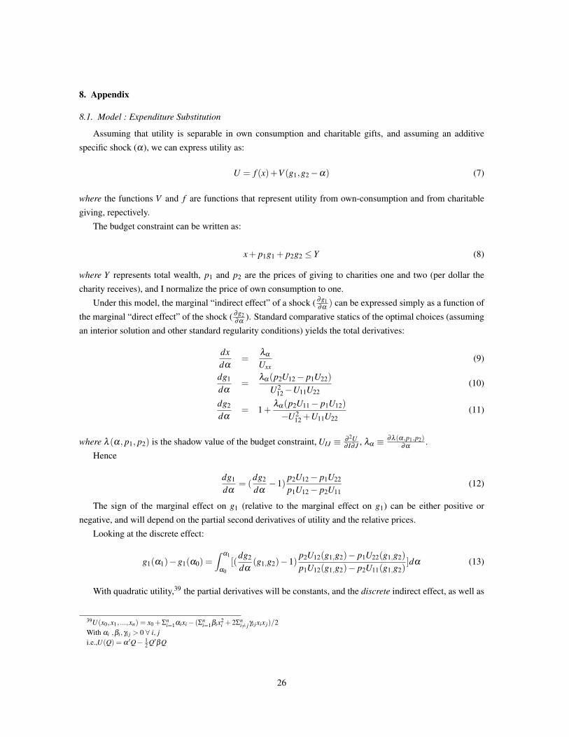
Assuming that utility is separable in own consumption and charitable gifts, and assuming an additivespecific shock (a), we can express utility as:

U = f (x)+V (g1,g2 �a) (7)

where the functions V and f are functions that represent utility from own-consumption and from charitablegiving, repectively.

The budget constraint can be written as:

x+ p1g1 + p2g2 Y (8)

where Y represents total wealth, p1 and p2 are the prices of giving to charities one and two (per dollar thecharity receives), and I normalize the price of own consumption to one.

Under this model, the marginal “indirect effect” of a shock ( ∂g1∂a ) can be expressed simply as a function of

the marginal “direct effect” of the shock ( ∂g2∂a ). Standard comparative statics of the optimal choices (assuming

an interior solution and other standard regularity conditions) yields the total derivatives:

dxda

=laUxx

(9)

dg1

da=

la(p2U12 � p1U22)

U212 �U11U22

(10)

dg2

da= 1+

la(p2U11 � p1U12)

�U212 +U11U22

(11)

where l (a, p1, p2) is the shadow value of the budget constraint, UIJ ⌘ ∂ 2U∂ I∂J , la ⌘ ∂l (a,p1,p2)

∂a .Hence

dg1

da= (

dg2

da�1)

p2U12 � p1U22

p1U12 � p2U11(12)

The sign of the marginal effect on g1 (relative to the marginal effect on g1) can be either positive ornegative, and will depend on the partial second derivatives of utility and the relative prices.

Looking at the discrete effect:

g1(a1)�g1(a0) =Z a1

a0[(

dg2

da(g1,g2)�1)

p2U12(g1,g2)� p1U22(g1,g2)

p1U12(g1,g2)� p2U11(g1,g2)]da (13)

With quadratic utility,39 the partial derivatives will be constants, and the discrete indirect effect, as well as

39U(x0,x1, ...,xn) = x0 +Sni=1aixi � (Sn

i=1bix2i +2Sn

i6= jgi jxix j)/2With ai ,bi,gi j > 0 8 i, ji.e.,U(Q) = a 0Q� 1

2 Q0bQ

26

the marginal effect, will be a simple linear function of the direct effect.

g1(a) = A+Bg2(a) (14)

where A and B are constants.Quadratic utility is often justified as a second-order approximation to any other utility function. With

other utility functions the partial derivatives may vary at different consumption bundles, so the indirect effectmay be a nonlinear function of the direct effect, but these should be solvable (equation 13) for a predictablefunctional form, which for estimation purposes, can be approximated to any desired accuracy by a polynomialfunction. In section 5.4 I estimate the response of the unshocked charities to the shocks as a function of theresponse of the shocked charities.

8.2. Further statistics

See, e.g., Andreoni and Gale, 1996.

27

Item Number Per centSingle, Never Married 46 82Married 5 9Divorced/Separated 4 7Don’t Want to Answer 1 2Total 56 100

(a) Marital status

Item Number Per centLost Data 5 5Male 43 44Female 49 51Total 97 100

(b) Sex

Item Number Per centDemocrat 34 44Republican 4 5Green Party 1 1Other Party 1 1No political affiliation 34 44Don’t want to answer 4 5Total 78 100

(c) Political affiliation

Item Number Per centAfrican American/Black 3 4Asian or Pacific Islander 47 60Don’t want to answer 6 8Hispanic/Latin 8 10Other/Mixed 6 8White/Caucasian 8 10Total 78 100

(d) Race/Ethnicity

Item Number Per centNot collected 19 20Catholic 15 15Protestant 7 7Other Christian 8 8Other Religion 14 14No preference/ No religion 28 29Don’t want to answer 6 6Total 97 100

(e) Religion

Item Number Per cent0-$10,000 7 9$10,000-$24,000 12 15$24,000-$41,000 14 18$41,000-$63,000 10 13$63,000-$94,000 8 10$94,000-$130,000 9 12$130,000-$200,000 4 5More than $200,000 6 8Don’t want to answer 8 10Total 78 100

(f) Income or parent’s income if dependent

Item Number Per centArts and humanities, psychology, legal studies 8 17business/ economics/ political science/ public policy 19 40Physical and life sciences / engineering / math 18 38Other 1 2Non-student 2 4Total 48 100

(g) College major

Table 7: Subject demographics and key characteristics

28

(a) (b)

(c) (d)

Figure 4: Example subjects: a. Flexible Purse, b. No crowding out, c. Flexible Purse, d. Relatively fixedpurse

29

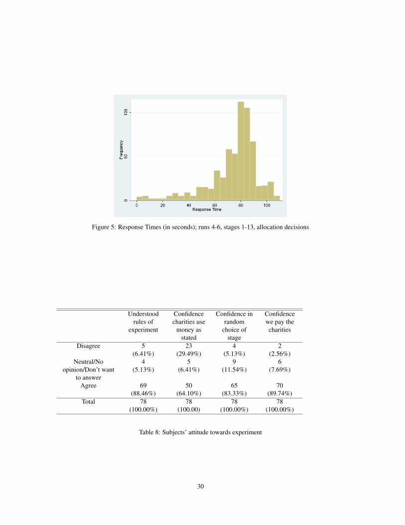
Figure 5: Response Times (in seconds); runs 4-6, stages 1-13, allocation decisions

Understoodrules of

experiment

Confidencecharities use

money asstated

Confidence inrandom

choice ofstage

Confidencewe pay thecharities

Disagree 5(6.41%)

23(29.49%)

4(5.13%)

2(2.56%)

Neutral/Noopinion/Don’t want

to answer

4(5.13%)

5(6.41%)

9(11.54%)

6(7.69%)

Agree 69(88.46%)

50(64.10%)

65(83.33%)

70(89.74%)

Total 78(100.00%)

78(100.00)

78(100.00%)

78(100.00%)

Table 8: Subjects’ attitude towards experiment

30

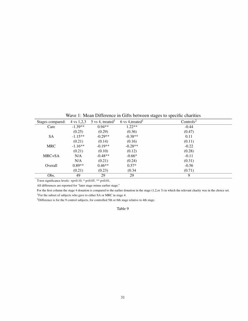
Wave 1: Mean Difference in Gifts between stages to specific charitiesStages compared: 4 vs 1,2,3 5 vs 4, treated1 6 vs 4,treated1 Controls2

Care -1.39** 0.94** 1.22** -0.44(0.25) (0.29) (0.36) (0.47)

SA -1.15** -0.29** -0.38** 0.11(0.21) (0.14) (0.16) (0.11)

MRC -1.16** -0.19** -0.28** -0.22(0.21) (0.10) (0.12) (0.28)

MRC+SA N/A -0.48** -0.66* -0.11N/A (0.21) (0.24) (0.31)

Overall 0.89** 0.46** 0.57* -0.56(0.21) (0.23) (0.34 (0.71)

Obs. 49 29 29 9T-test significance levels: +p<0.10, * p<0.05, ** p<0.01,All differences are reported for “later stage minus earlier stage.”For the first column the stage 4 donation is compared to the earlier donation in the stage (1,2,or 3) in which the relevant charity was in the choice set.1For the subset of subjects who gave to either SA or MRC in stage 4.2Difference is for the 9 control subjects, for controlled 5th or 6th stage relative to 4th stage.

Table 9

31

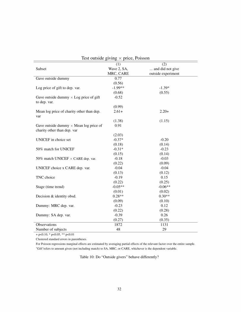
Test outside giving ⇥ price, Poisson(1) (2)

Subset Wave 2, SA, ... and did not giveMRC, CARE outside experiment

Gave outside dummy 0.77(0.56)

Log price of gift to dep. var. -1.99** -1.39*(0.68) (0.55)

Gave outside dummy ⇥ Log price of giftto dep. var.

-0.52

(0.99)Mean log price of charity other than dep.var

2.61+ 2.20+

(1.38) (1.15)Gave outside dummy ⇥ Mean log price ofcharity other than dep. var

0.91

(2.03)UNICEF in choice set -0.37* -0.20

(0.18) (0.14)50% match for UNICEF -0.31* -0.23

(0.15) (0.14)50% match UNICEF ⇥ CARE dep. var. -0.18 -0.03

(0.22) (0.09)UNICEF choice x CARE dep. var. -0.04 -0.04

(0.13) (0.12)TNC choice -0.19 0.15

(0.22) (0.25)Stage (time trend) -0.05** -0.06**

(0.01) (0.02)Decision & identity obsd. 0.28** 0.30**

(0.09) (0.10)Dummy: MRC dep. var. -0.23 0.12

(0.22) (0.28)Dummy: SA dep. var. -0.39 0.26

(0.27) (0.35)Observations 1872 1131Number of subjects 48 29+ p<0.10, * p<0.05, ** p<0.01Clustered standard errors in parentheses.For Poisson regressions marginal effects are estimated by averaging partial effects of the relevant factor over the entire sample."Gift"refers to amount given (not including match) to SA, MRC, or CARE, whichever is the dependent variable.

Table 10: Do “Outside givers” behave differently?

32

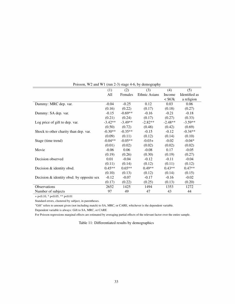
Poisson, W2 and W1 (run 2-3) stage 4-6, by demography(1) (2) (3) (4) (5)All Females Ethnic Asians Income Identified as

< $63k a religionDummy: MRC dep. var. -0.04 -0.25 0.12 0.03 0.06

(0.16) (0.22) (0.17) (0.18) (0.27)Dummy: SA dep. var. -0.15 -0.69** -0.16 -0.21 -0.18

(0.21) (0.24) (0.17) (0.27) (0.33)Log price of gift to dep. var. -3.42** -3.49** -2.82** -2.48** -3.59**

(0.50) (0.72) (0.48) (0.42) (0.69)Shock to other charity than dep. var. -0.30** -0.35** -0.15 -0.12 -0.34**

(0.09) (0.11) (0.12) (0.14) (0.10)Stage (time trend) -0.04** -0.05** -0.03+ -0.02 -0.04*

(0.01) (0.02) (0.02) (0.02) (0.02)Movie -0.06 0.06 -0.08 0.17 -0.05

(0.19) (0.26) (0.30) (0.19) (0.27)Decision observed 0.01 -0.04 -0.12 -0.11 -0.04

(0.11) (0.14) (0.12) (0.11) (0.12)Decision & identity obsd. 0.45** 0.65** 0.49** 0.43** 0.47**

(0.10) (0.13) (0.12) (0.14) (0.15)Decision & identity obsd. by opposite sex -0.12 -0.07 -0.17 -0.16 -0.02

(0.17) (0.22) (0.25) (0.13) (0.20)Observations 2652 1425 1494 1353 1272Number of subjects 97 49 47 43 44+ p<0.10, * p<0.05, ** p<0.01Standard errors, clustered by subject, in parentheses."Gift" refers to amount given (not including match) to SA, MRC, or CARE, whichever is the dependent variable.Dependent variable is always: Gift to SA, MRC, or CAREFor Poisson regressions marginal effects are estimated by averaging partial effects of the relevant factor over the entire sample.

Table 11: Differentiated results by demographics

33

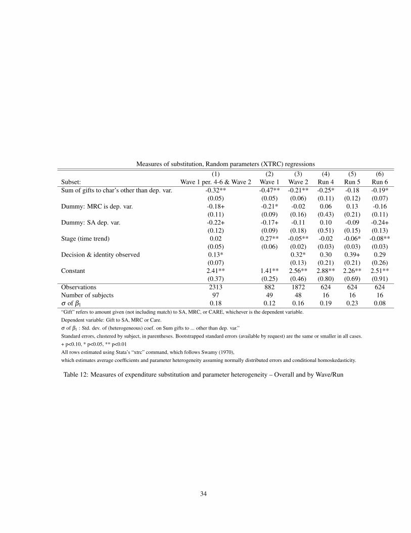
Measures of substitution, Random parameters (XTRC) regressions(1) (2) (3) (4) (5) (6)

Subset: Wave 1 per. 4-6 & Wave 2 Wave 1 Wave 2 Run 4 Run 5 Run 6Sum of gifts to char’s other than dep. var. -0.32** -0.47** -0.21** -0.25* -0.18 -0.19*

(0.05) (0.05) (0.06) (0.11) (0.12) (0.07)Dummy: MRC is dep. var. -0.18+ -0.21* -0.02 0.06 0.13 -0.16

(0.11) (0.09) (0.16) (0.43) (0.21) (0.11)Dummy: SA dep. var. -0.22+ -0.17+ -0.11 0.10 -0.09 -0.24+

(0.12) (0.09) (0.18) (0.51) (0.15) (0.13)Stage (time trend) 0.02 0.27** -0.05** -0.02 -0.06* -0.08**

(0.05) (0.06) (0.02) (0.03) (0.03) (0.03)Decision & identity observed 0.13* 0.32* 0.30 0.39+ 0.29

(0.07) (0.13) (0.21) (0.21) (0.26)Constant 2.41** 1.41** 2.56** 2.88** 2.26** 2.51**

(0.37) (0.25) (0.46) (0.80) (0.69) (0.91)Observations 2313 882 1872 624 624 624Number of subjects 97 49 48 16 16 16s of b1 0.18 0.12 0.16 0.19 0.23 0.08“Gift” refers to amount given (not including match) to SA, MRC, or CARE, whichever is the dependent variable.Dependent variable: Gift to SA, MRC or Care.s of b1 : Std. dev. of (heterogeneous) coef. on Sum gifts to ... other than dep. var.”Standard errors, clustered by subject, in parentheses. Bootstrapped standard errors (available by request) are the same or smaller in all cases.+ p<0.10, * p<0.05, ** p<0.01All rows estimated using Stata’s “xtrc” command, which follows Swamy (1970),which estimates average coefficients and parameter heterogeneity assuming normally distributed errors and conditional homoskedasticity.

Table 12: Measures of expenditure substitution and parameter heterogeneity – Overall and by Wave/Run

34

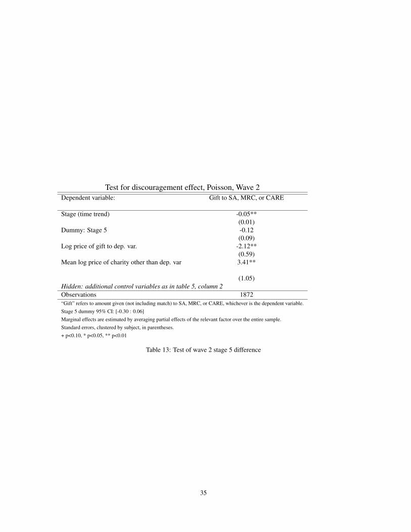
Test for discouragement effect, Poisson, Wave 2Dependent variable: Gift to SA, MRC, or CARE

Stage (time trend) -0.05**(0.01)

Dummy: Stage 5 -0.12(0.09)

Log price of gift to dep. var. -2.12**(0.59)

Mean log price of charity other than dep. var 3.41**

(1.05)Hidden: additional control variables as in table 5, column 2Observations 1872“Gift” refers to amount given (not including match) to SA, MRC, or CARE, whichever is the dependent variable.Stage 5 dummy 95% CI: [-0.30 : 0.06]Marginal effects are estimated by averaging partial effects of the relevant factor over the entire sample.Standard errors, clustered by subject, in parentheses.+ p<0.10, * p<0.05, ** p<0.01

Table 13: Test of wave 2 stage 5 difference

35