Substitutes or Complements?Alcohol, Cannabis and Tobacco.

Lisa CameronDepartment of EconomicsUniversity of Melbourne

and

Jenny Williams*

School of EconomicsUniversity of Adelaide

12 July 1999.

Abstract

This paper estimates the price responsiveness of cannabis, alcohol and cigarette use.Individual level data from four waves of the National Drug Strategy Household Survey aremerged with previously unavailable state level data on cannabis prices, and ABS alcohol andtobacco price indices. In addition to own price effects, we estimate cross price effects and theimpact of differing legal regimes for cannabis on the use of these three drugs. Establishingthe nature of the interdependencies between cannabis, alcohol and cigarettes is important inthe development of drug policy so that a policy directed at one drug does not unintentionallyaffect the demand for other drugs. We find that participation in the use of all three drugs isresponsive to own prices and that decriminalisation of cannabis leads to higher cannabis use.Cannabis is found to be a substitute for alcohol and a complement to tobacco. Alcohol andtobacco are found to be complements.

JEL: D1, I1

Key words: drug use, price responsiveness, participation, decriminalisation.

* We would like to thank Hank Prunken for the cannabis price data and Steve Whennan for the unpublishedABS alcohol and tobacco price data. We are also grateful to Chris Skeels and the Department of Statistics at theAustralian National University for hosting Dr Williams as a visitor when work on this project commenced. Thispaper benefited from the comments of Frank Chaloupka and Joe Hirschberg. We gratefully acknowledgefinancial support from ARC grant No. 4222/98.

1

I. Introduction

This study investigates the use of three commonly used drugs in Australia: cannabis,

alcohol and tobacco. In particular, we seek to determine the responsiveness of drug use to

each drug’s own price, and the price of the other drugs. We also examine the extent to which

criminal status impacts upon drug use. These issues are key to drug policy development. For

example, if cannabis use is negatively related to its price, then deterring use through price

provides an alternative policy instrument to the criminal justice system. The use of price

rather than criminal sanctions may offer substantial social benefits. As is often noted,

criminalising cannabis use groups it with the more socially harmful illicit drugs This leaves

users of cannabis at greater risk of exposure to sellers of harder illicit drugs, and the attendant

criminal activity. These undesirable consequences could be avoided by policies which

regulate cannabis use through the price system, rather than the criminal justice system.

Notwithstanding their licit status, alcohol and cigarette use are also subject to

regulation. While these regulations are developed to address the use of each drug separately,

there is reason to believe that the demand for cannabis, alcohol and cigarettes may be

interrelated. Tobacco and cannabis share smoking as the route of administration, while the

effect of alcohol use resembles cannabis in terms of its intoxicating and euphoric effects.

Understanding the interdependencies of demand for various drugs is important to ensure that

a policy aimed at influencing the use of one drug does not have unintended consequences for

the use of other drugs.

Despite the increased awareness of the harm associated with drinking and smoking,

and the emergence of drug policy as a central issue facing legislators, very little has been

written on the demand for alcohol, tobacco and cannabis in Australia. The Australian

literature that does exist has used time-series data to examine the demand for alcohol

(Clements, Yang and Zheng, 1997) and tobacco (Bardsley and Olekalns, 1998). There have

been no studies that use micro-data for this purpose and the time-series studies do not attempt

2

to look at cross-price elasticities. The only studies of an economic nature that examine illicit

drug use in Australia are attempts to quantify the costs and benefits of Australian Drug Policy

(Marks, 1991 for example). This study attempts to overcome this shortcoming in the

literature by examining alcohol, cigarette and cannabis use in Australia.

Cannabis prices are the key to being able to study the interdependence between

cannabis and legal drug use. In this study we use previously unavailable data on cannabis

prices which were provided by the State Commissioners of Police. We merge state level

cannabis price data with individual level observations on drug use from four waves of the

National Drug Strategy Household Surveys. The data cover the years 1988, 1991, 1993 and

1995 and each Australian State and Territory. We also use Australian Bureau of Statistics

(ABS) state level data on the consumer price indices for alcohol and tobacco. A comparison

of South Australia and the other states allows us to examine the effect of decriminalisation of

cannabis. In 1987 South Australia reduced the legal sanctions against the possession of small

amounts of cannabis. The ACT followed suit in 1992 as did the Northern Territory in 1996.1

In 1999 Victoria also moved to a system of partial prohibition. Given the current policy

climate, our research is both important and timely.

The rest of the paper is organised as follows. In Section 2 we survey the empirical

literature on illicit drug use and the substitutability between cannabis, alcohol and cigarettes.

Section 3 discusses the legal sanctions against cannabis use in Australia. Section 4 discusses

the data. In Section 5 the methodology is introduced and the results are discussed in Section

6. Section 7 concludes.

I. Previous Literature

An empirical literature based on studies from the U.S. has sought to establish the

relationship between alcohol, tobacco and cannabis, and the effect of various government

1 While the ACT also introduced a system of expiation for minor cannabis offences during the period underanalysis, no price data was obtained for cannabis. Therefore, we omit the ACT from our analysis. The Northern

3

policies on the use of these drugs. Interestingly, these studies do not typically use data on

cannabis prices, since this data is not consistently available. In the absence of price data,

much of the literature includes policy variables such as decriminalisation of cannabis,

drinking age laws, and taxes on alcohol and cigarettes to capture the full price of these drugs.

The U.S. evidence regarding the relationship between alcohol and cannabis use is

mixed. The earliest studies found alcohol and cannabis to be substitutes. DiNardo and

Lemieux (1992) merged data on youth drug use with data on legal drinking age laws, the

price of alcohol and a variable indicating cannabis decriminalisation. Drinking age laws were

found to have a significant positive effect on cannabis participation, while decriminalisation

had a significant negative effect on alcohol use. They concluded on this basis that the two

drugs were substitutes, although the price of alcohol was found to have no effect on cannabis

use. In a series of papers, Model (1992, 1993) reached a similar conclusion. She based this

on the observation that a high percentage of violence in the U.S. is alcohol-related and that

U.S. states with more liberal cannabis laws have lower violent crime rates, particularly

homicide rates (Model, 1992), and less (non-cannabis related) emergency room episodes

(Model, 1993).

Other studies have however concluded that alcohol and cannabis use have a

complementary relationship. For example, Thies and Register (1993) combine data on youth

drug use, drinking age laws and decriminalisation indicators to measure the full price of

alcohol and cannabis respectively. They find that individuals who live in states where the use

of cannabis is decriminalised are more likely to use alcohol.2 Saffer and Chaloupka (1998),

using nationally representative household surveys on drug use, found a negative relationship

between cannabis use and the price of alcohol and so also concluded that they are

complements. However, decriminalisation was found to have no effect on alcohol use.

Territory is excluded for the same reason. 2 They also find that drinking age laws have no effect on cannabis use.

4

There have also been conflicting findings within studies. Pacula (1988a) found that

although youths in states which had decriminalised the use of cannabis had lower rates of

alcohol use, indicating that the two goods are substitutes, states with higher taxes on beer had

lower levels of cannabis use, indicating complementarity. Mixed findings are also reported

by Chaloupka and Laixuthai (1997). Their study of youth finds that cannabis

decriminalisation reduces alcohol use, and that alcohol use is positively related to the

wholesale price of cannabis, suggesting the two drugs are substitutes. However, a

complementary relationship is implied when the retail price of cannabis is used. Farrelly,

Bray, Zarkin, Wendling and Pacula (1999) find a negative relationship between alcohol prices

and cannabis use for youth but not for adults.

The literature on the interdependency between cannabis and tobacco use is far more

limited. There are only two studies of which we are aware. Chaloupka, Pacula, Farrelly,

Johnston, O’Malley, and Bray (1999) augment individual level data with state level

information on jail sentences and fines for cannabis use to measure the full price of cannabis,

the money price of cigarettes and tobacco control policies to measure the full price of

cigarettes. The variables related to the full price of cannabis are not significant in the cigarette

use equation, nor is the price of cigarettes significant in the cannabis participation equation.

However, the price of cigarettes is found to have a negative and significant effect on the

average level of cannabis used. Similarly, Farrelly et al. (1999) report the price of cigarettes

to have a negative effect on cannabis use, but these results are only significant for youth and

not for adults.

In addition to the interdependencies between cannabis, alcohol, and cigarette use, the

studies discussed above examine the effect of the legal status, fines and sentences on cannabis

use. In general, studies based on youths find no effect of criminal status on cannabis use

(DiNardo and Lemieux, 1992; Thies and Register, 1993; Pacula, 1998; Farrelly et al., 1999),

while studies based on adults and youth, or just adults tend to find that decriminalisation

5

increases cannabis use (Model, 1993; Saffer and Chaloupka, 1998), and that cannabis use is

negatively related to fines and sentences (Farrelly et al., 1999).

While we are aware of no research in Australia which examines the relationship

between the price of cannabis and its use, there have been a series of reports into the impact

of the system of expiation on cannabis use in South Australia using the National Drug

Strategy Household Surveys (Christie, 1991; Donnelly and Hall, 1994; Donally, Hall and

Christie, 1995; Ali, Christie, Lenton, Hawks, Sutton, Hall and Allsop, 1998). These reports

found no evidence of an increase in the population rates of cannabis use in South Australia

relative to the rest of Australia up until 1993. However, Ali, Christie, Lenton, Hawks, Sutton,

Hall and Allsop, (1998) find that a comparison between 1985 and 1995 indicates an increase

in self-reported lifetime cannabis use in South Australia relative to the average of other states.

They conclude that the increase is unlikely to be due to the introduction of the system of

cannabis expiation notices (CEN) on the basis of three observations. First, similar increases

in reported lifetime use occurred in Tasmania and Victoria, where there was no change in the

legal status of the drug. Second, there was no change in weekly cannabis use in South

Australia relative to the average for Australia, and third, there was no increase in cannabis use

among young adults aged 14-19 in South Australia relative to the average of the other states.

II. Australian Cannabis History

Australia’s policy on cannabis has been guided by the numerous international

conventions to which it is a signatory.3 The 1925 Geneva Convention on Opium and Other

Drugs required that cannabis availability and use be limited to medical and scientific

purposes. This convention remains in force today, with a legislative system of total

prohibition as the most common status of cannabis in the international community.4 Under

total prohibition, possession, cultivation, importation, sale and distribution of any amount of

3 The United States has been a major influence in developing and promoting these conventions. 4 The Netherlands is an exception. Cannabis receives less punitive treatment compared to other drugs, with

6

cannabis is prohibited, and the law is enforced with criminal penalties which may include

imprisonment and fines. A number of committees of inquiry into drug use and trafficking in

Australia have rejected the legislative model of total prohibition, recommending the removal

of criminal penalties for offences relating to the personal use of cannabis.5 The basis of this

recommendation has been the undesirable and unintended consequences associated with the

imposition of total prohibition of cannabis. Under total prohibition with criminal penalties,

the market for cannabis is a black market, characterised by higher prices and profits relative

to a legal competitive market. These features of the market make selling cannabis more

attractive to providers of harder drugs, bringing consumers of cannabis into contact with these

more dangerous drugs. Also, the higher prices may induce crimes of acquisition for the

purpose of obtaining money for buying cannabis. Further, it is perceived that the harm

imposed on cannabis users by way of a criminal record, and the imposition of fines and

imprisonment, outweighs the social harm of cannabis use.

In particular, the concern over separating cannabis markets from harder drug markets

has led several state legislators to liberalise the legal status of cannabis. The first state to do

so was South Australia, where a system of expiation was adopted in 1987. The Report of the

National Task Force on Cannabis (1994) describes expiation as prohibition with civil

penalties. Under this model, possession and cultivation of small amounts of cannabis for

personal use is dealt with by civil penalties such as fines, rather than court imposed fines or

imprisonment. Criminal sanctions still apply to the possession, cultivation and distribution of

large quantities of cannabis. Similar schemes have also been introduced in the ACT in 1992,

and the Northern Territory in 1996. Victoria has recently moved to a system of partial

prohibition. Under this system, controls on the production and distribution of commercial

small quantities of cannabis products (hashish and marijuana), being legally sold in ‘youth centres’ and ‘coffeeshops’ to individuals over the age of 16. 5 The most recent of these inquiries was carried out by the National Task Force on Cannabis (1994).

7

quantities remain, but cannabis use, or the possession of small quantities for person use is not

an offence.

III. Data

The data used in this research are drawn from the National Drug Strategy Household

Surveys (NDSHS) for the years 1988, 1991, 1993 and 1995.6 The NDSHS was initiated by

the Drugs of Dependence Branch of the Federal Department of Human Services and Health

and is designed to provide data on the extent of drug use by the non-institutionalised civilian

population aged fourteen years and older in Australia7. To minimise under reporting of drug

use, respondents filled out a sealed section of the questionnaire which allowed them to

indicate their level of drug use without the interviewer being aware of their answers.8 Both

legal and illegal drugs are included. In this study we pool the cross-sections into one data set,

resulting in a sample size of 9,744.

The three dependent variables used in our analysis are indicators for use of cannabis,

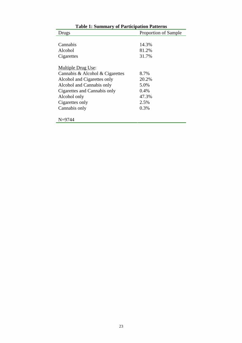
alcohol or cigarettes in the last twelve months. Table 1 provides some summary statistics of

participation behaviour. 14.3% of the sample report that they have used cannabis in the last

12 months. 81.2% have consumed an alcoholic beverage and 31.7% are cigarette smokers.

The table also illustrates the close relationship between cannabis use and the use of the other

drugs. 96% of cannabis users also drink alcohol. 63.6% of cannabis users are cigarette

smokers. Only 2% (0.3% of the entire sample) use cannabis but neither of the two other

substances. Interestingly only 2.8% of cannabis users are smokers but not drinkers. This

suggests that the relationship between cannabis and alcohol is closer than that between

cigarettes and cannabis. Alcohol and cannabis may meet the same needs.

6There is also a 1985 survey but the questionnaire in that year differed in such a way to make it inappropriate forthis study. 7 We drop individuals aged over 70 from the sample. 8 Surveys of illicit drug use probably underestimate the prevalence of use. Illicit drug users may be under-sampled in household surveys because they are more heavily represented in populations not included in thesurveys, and those who are contacted may be reluctant to take part for fear of legal consequences of admitting anillegal act. Also, those users who take part in the survey are likely to underestimate frequency of use and

8

In addition to use drug use, detailed socioeconomic and demographic information is

collected in the surveys.9 We include as potential determinants of drug use the following

individual specific variables: age, gender, marital status, the presence of children in the

household, an indicator for still in school, highest level of education attained, and an indicator

for residing in a capital city. A full definition of variables and descriptive statistics is given in

the appendix.

The individual level survey data is merge with price data which varies by state and

year. The alcohol and tobacco prices are from the Consumer Price Index, Tobacco and

Alcohol: Group, Subgroup and Expenditure Class Index Numbers. This unpublished, state

level quarterly data for the cigarettes and tobacco subgroup and alcoholic drinks subgroup

was provided by the Australian Bureau of Statistics. In addition to this we have quarterly

cannabis price data for each state.10 These data were previously unavailable and have been

supplied by the State Commissioners of Police. The price are those elicited by police during

undercover buys. We have prices for purchases of grams and pounds of “head” which is the

flowering top of the cannabis plant and has the highest concentration of the active ingredient,

THC, and also for grams and pounds of “leaf” which is the chopped leaf of the plant. All

prices are converted into real prices by dividing by the CPI. We convert the four price series

to an annual standardised cannabis price, as is described below.

Standardising Prices

Following the method outlined in Saffer and Chaloupka (1995), we construct the

standardised cannabis price by regressing the log of price, MARIJjtP , on a dummy variable,

pound, that equals 1 if the price is for a pound of the drug and 0 if it is for a gram of the drug,

amounts used. One means of minimising these problems is to assure confidentiality for participants in thesurvey. 9 Some, but not all years provide individual and household income data. 10 We only have limited data for the Australian Capital Territory (ACT) and the Northern Territory (NT) and soexclude individuals in these localities from the sample.

9

a dummy variable, head, that equals 1 if the price is for “head” and 0 for “leaf”. We also

include vectors of state and year dummies.

jttjjtjtMARIJjt yearstateheadpoundP εββββα +++++= 4321 (1)

We then predict the price of a gram of head quality cannabis in each year for each of

the states using the coefficients that result from OLS estimation of equation 1. This is the

cannabis price that is used in the participation equations estimated below. It is worth noting

that by estimating the prices in this way we also eradicate any concern associated with the

possible endogeneity of the prices. The use of predicted prices removes any correlation that

may have existed between the actual prices and the error term in the participation equation.

IV. Method

Following standard consumer theory, we model individuals as maximising utility

subject to a budget constraint. We assume that utility is a function of the amount of each good

consumed and partition the choice set of goods into D, which consists of the drugs, alcohol,

cigarettes and cannabis; and the remaining goods X. The maximisation problem is thus:

INCXPDPXDUMax XD

XD≤+ .. s.t. ),(

,

where INC is the individual’s disposable income, PD is the vector of drug prices and PX is the

vector of prices for all other goods.11 In modelling illicit drug use, we control for the full price

of the drug, as opposed to just the money price. The full price reflects the additional cost

associated with legal and social sanctions against drug use. We adopt a general specification

that allows the legal status to affect cannabis use directly, and indirectly through

responsiveness to money price. The former effect is captured using a dichotomous indicator

that reflects the criminal nature of cannabis use in the individual’s place of residence. CRIM

11 This formulation ignores the dynamic aspect of consumption and so does not recognise the addictive characterof the legal and illegal drugs. This is an extension worthy of further research.

10

equals 1 if cannabis is illicit and zero if licit. The latter effect is modelled by interacting the

money price of cannabis with the indicator CRIM.

The individual’s problem can be expressed by the Lagrangean equation:

)..(),( INCXPDPXDUZ XD −++= λ (2)

Solving for the optimal choice of X and D and allowing for corner solutions produces the

following first order conditions:

0

1,....K.kfor 0 and 0 ,0

1,.....Jjfor 0 and 0 ,0

=∂∂

==∂∂≥≤

∂∂

==∂∂≥≤

∂∂

λZ

x

Zxx

x

Z

D

ZDD

D

Z

kkk

k

jjj

j

(3)

Hence, if the individual engages in the use of drug j,

0 and 0 =∂∂>

jj D

ZD

where

jj DD

jj

PPD

U

D

Z λλ −=∂∂+

∂∂=

∂∂

jD

U so and (4)

This is just the standard optimisation condition which states that the individual

consumes to the point where the marginal utility of consumption equals the marginal

disutility associated with foregoing goods that would otherwise have been bought and

consumed.

However it is also possible that :

jDj

j

PDD

Z λ−<∂∂⇒=>

∂∂

jD

U 0 ,0 (5)

11

In this case we have a corner solution and the individual does not consume any of the

jth drug because higher utility is attained by allocating resources to the consumption of the

other goods. In this case the individual does not participate in the use of this particular drug.

The demand for each of the drugs, Dj , is hence a function of the (full) price of each

good relative to the other goods. Because we are focusing on the consumption of drugs we

have implicitly included the price of other goods by normalising the drug prices with respect

to the CPI. We include interactions between the different prices in the empirical analysis to

allow for the most flexible functional form. Dj will also be a function of individual income,

and variables that affect the utility function of the individual.

We can thus write:

( ) ( )( )

j

jMARIJMARIJCIG

MARIJALCCIGALCMARIJCIGALCj

ex

eYPCRIMCRIMPP

PPPPPPPD

+′=

++×++×

×+×++++=

βηγγγ

γγγγγαˆˆˆ

ˆˆˆˆˆˆˆ

876

54321

(6)

where j={alcohol, cigarettes, cannabis},Y is a vector of demographic variables that are likely

to be correlated with individuals’ tastes and ej is a standard normal random variable. In the

analysis below the vector Y consists of the age of the individual, gender, marital status,

presence of children in the household, educational attainment and whether the individual lives

in a capital city. Unfortunately most years of the NDSHS do not provide data on individual or

household income. Income would enter the participation index via the budget constraint and

might also affect people’s tastes. Although we can’t control for income in this study, its effect

is captured by those demographic variables that are correlated with income: age, education,

gender and capital city residency. In addition to picking up differences in tastes across age

groups, the age variables may also pick up the effect of changes in availability and trends in

drug use over time.

In this paper, we focus on the decision to use cannabis, alcohol and tobacco, and not

on the frequency of use. Therefore, our dependent variable is

12

I if D

if D

j j

j

= >= ≤

1 0

0 0

where Ij, is an indicator for the unobserved level demand for good j, Dj, and we refer to ′β x

as the underlying participation index. Note that:

( ) ( )

( ).00

xF

exPDP jj

ββ

′=

>+′=>

We assume F to be the standard normal distribution function and so participation in drug use

has the standard probit formulation.

V. Results

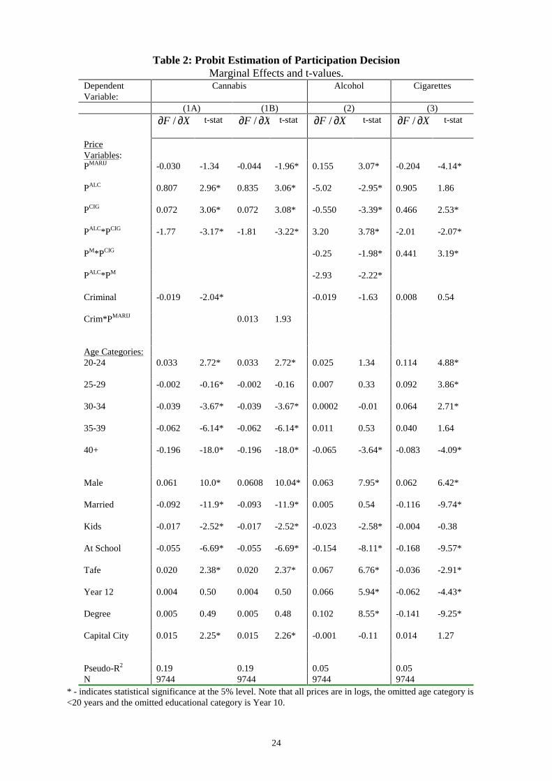
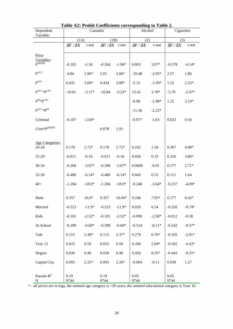
Table 2 presents the probit estimates of the participation equations for cannabis,

alcohol and cigarettes. To aid interpretation only the marginal effects and their t-statistics are

reported. The probit coefficients are shown in Table A2 in the appendix. 12 The marginal

effects are interpreted as the change in the probability of participation that results from a one

unit increase in a continuous variable and from a change from zero to one for dummy

variables. We will first focus on the price effects and later summarise the effects of the

demographic variables.

General to specific modelling was used to arrive at the preferred model for each drug.

The most general model included a full set of price interaction variables. If the interaction

terms were insignificant, they were dropped from the specifications reported in Table 2.

Own Price Elasticities

As discussed above, it is important to control for the full price of an illicit drug when

modelling its demand. The full price includes the expected legal and social sanctions

associated with drug use. The routine way to control for the full price is to include a dummy

12 The probit coefficients represent the contribution of the explanatory variables to the underlying participation

13

variable that reflects the legal status of the drug (CRIM =1 if the drug is illicit and 0 if

decriminalised). This is the approach taken in column (1A) of Table 2. In Column (1B) we

allow criminalisation to operate via the price mechanism by the inclusion of the variable

(CRIM x PMARIJ). This allows criminalisation to affect the responsiveness of use to the money

price. It may be that when illicit, even very low money prices will not greatly induce

participation, but that when legal sanctions are relaxed, price changes will result in

behavioural changes. Ideally one would like to include both CRIM and (CRIM x PMARIJ).

However, in the current context these two terms are very highly correlated and

multicollinearity results. The approach taken here is to control for each separately and report

both sets of results.

One further point bears mentioning before interpreting the estimation results. In

practice, our indicator for criminal status of cannabis is identical to a (1-South Australian

dummy variable) because South Australia was the only state to have relaxed legal sanctions

against cannabis included in our sample. The indicator CRIM is intended to account for the

impact of cannabis laws on drug use. It is conceivable, however, that other differences

between South Australia and the rest of Australia, such as prevailing attitudes and behaviours,

are being picked up by this variable.

Columns (1A) and (1B) of Table 2 report the results for the participation in cannabis

use equation including CRIM and (CRIM x PMARIJ) respectively. Only the price interaction

term (PALCxPCIG) was statistically significant, so the others were dropped. The coefficient on

the variable CRIM in column (1A) shows that cannabis participation is on average 1.9

percentage points lower in states in which use is a criminal offence. The price of cannabis is

negatively correlated with participation but is not statistically significant.

However, the results in Column (1B) suggest that cannabis use is price responsive. In

states where cannabis has been decriminalised a 1% increase in the real price of cannabis

index and are ordinal rather than cardinal.

14

decreases the probability of participation by 0.044 percentage points, and this effect is

statistically significant.13 When the drug is illicit, then the price effect is the sum of the

coefficient on PMARIJ and (CRIM x PMARIJ). The resulting point estimate suggests that the

probability of participation decreases 0.031 percentage points in response to a 1% increase in

price. This accords with intuition, since under a harsh penalty regime one might reasonably

expect that demand would be less responsive to money prices because the money price is a

smaller component of the full price.

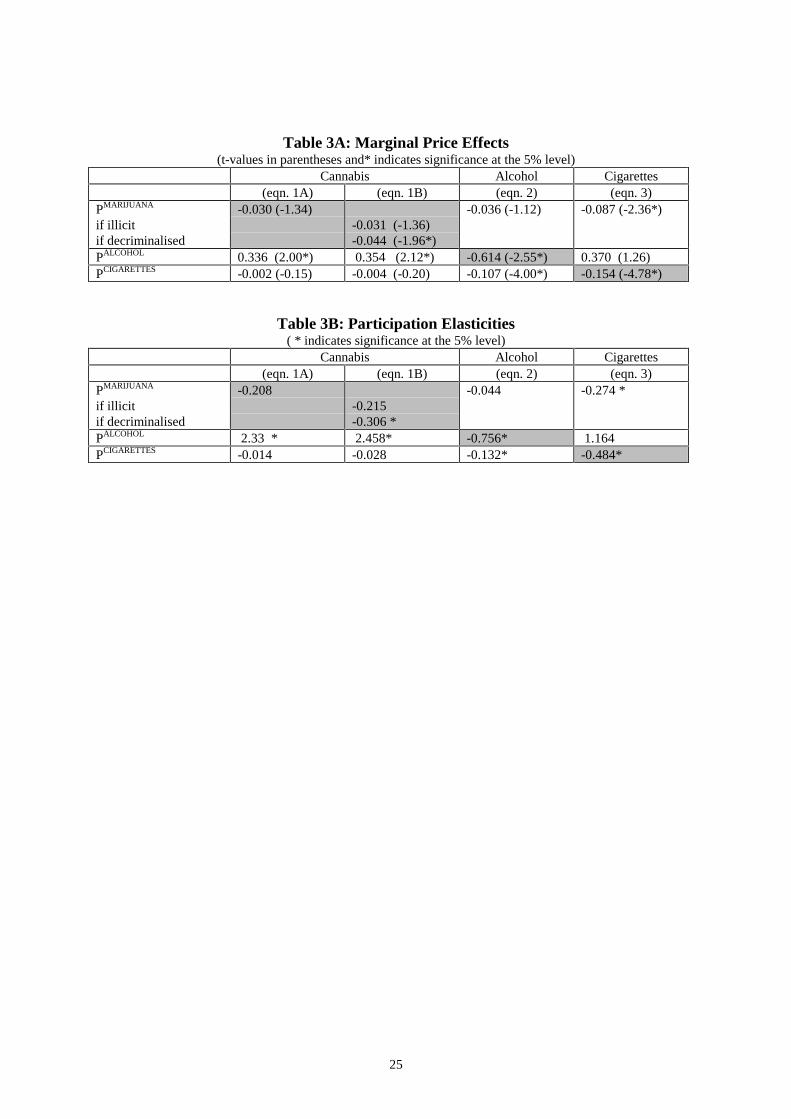
Column 1A and 1B of Table 3A summarise the total marginal effect of price on

cannabis use and the corresponding t-stats. Column 1B shows that the responsiveness of use

to own price in states where it is a criminal offence is insignificantly different from zero. This

suggest that participation may not be price responsive at all in states where the possession of

small quantities is a criminal offence. This is consistent with the insignificant coefficient on

PMARIJ in model (1A) since this coefficient captures only the average price effect across the

six states, of which only one state has decriminalised cannabis use. The lack of price

responsiveness in the other five states dominates the model (1A) result.

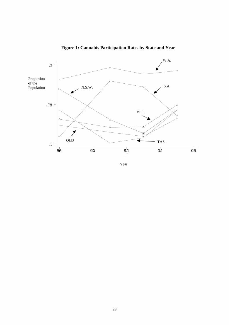
Models 1A and 1B are also consistent in terms of predicting that participation is

highest in South Australia. This is because, although decriminalisation increases price

responsiveness of cannabis use, South Australia enjoys much lower cannabis prices relative to

the other states. The latter effect dominates to the extent that model (1B) predicts

participation to be the greatest in South Australia in accordance with model (1A). The

average participation rate in SA is 2.5 percentage points higher than Victoria’s, 2.1

percentage points higher than for WA, 2.0 percentage points higher than for NSW, 1.7

percentage points higher than for Queensland and 1.2 percentage points higher than in

Tasmania.

13 Note that the price terms are all measured in logs and so the marginal effects are the change in theparticipation probability for a 100% increase in the variable in levels.

15

In summary, we do not reject the hypothesis that cannabis use is price responsive once

legal sanctions have been liberalised. This price responsiveness combined with lower prices

in South Australia (which are possibly a result of this liberalisation) have induced higher

participation. The finding that decriminalisation coincides with higher participation rates is

consistent with the U.S. studies although the magnitude of the effect is larger here.14

Columns 2 and 3 of Table 2 report the results of the alcohol and cigarette participation

equations. Again some price interaction terms were not significant and were dropped. For

both legal drugs we control for the effect of the legal status of cannabis through the inclusion

of the dummy variable CRIM.15 The results provide no evidence that the criminal status of

cannabis use has a direct effect on participation in alcohol or cigarette use.16 Our findings with

respect to alcohol and cigarette use are consistent with the findings of Saffer and Chaloupka

(1998), and Chaloupka, Pacula, Farrelly, Johnston, O’Malley and Bray (1999).

Both alcohol and cigarette use are clearly own-price responsive. The inclusion of the

price interaction terms makes it difficult to assess the total marginal effect of say an increase

in the price of alcohol on alcohol consumption by just examining the individual marginal

effects in Table 2. To aid interpretation Table 3A reports the total marginal effects of price

changes in each of the equations.17 A 1% increase in the real price of alcohol decreases the

probability of participation by 0.61 percentage points. A 1% increase in the real price of

cigarettes decreases the probability of smoking by 0.15 percentage points.

14 As mentioned in Section 2, Saffer and Chaloupka (1995) found that decriminalisation in the U.S. led toincreased participation in the range of 4 to 7%. Our result shows participation increasing 0.019/0.144=13.2%.15 We experimented with instead including CRIM x PMARIJ but the reported models fit the data better.16 Column (2) shows that on average alcohol participation is lower (1.9 percentage points) in states where useremains a criminal offence, although this effect is statistically insignificant. This is identical in magnitude to thepredicted decrease in cannabis participation in these states. Although we should not make too much of astatistically insignificant result, as discussed earlier, we cannot differentiate between the effects ofdecriminalisation and prevailing attitudes and behaviours in South Australia. That is to say, we may be detectinga “South Australia” effect rather than a “decriminalisation” effect. Since other states have subsequentlyliberalised laws on the use of cannabis, this is an issue that can be addressed in the future when data on thesestates can be utilised to better identify the effects of these laws.17 Note that the marginal effect of a change in the price of alcohol, for example, is calculated as

MMALCCIGALCALC

PPPP

F

PP

F

P

F CIG . . )*()*( ∂

∂∂

∂∂

∂++ = -5.02 + 3.20 x 0.27 – 2.93 x –1.214.

16

Table 3B converts all of the price effects to participation elasticities. This allows a

comparison of the magnitude of the own price effects, standardising for the mean level of use

and allows a comparison with the results of previous studies which often report their results

in terms of elasticities.18 The participation elasticities are –0.306 for decriminalised cannabis,

-0.756 for alcohol and–0.484 for cigarettes. These are in the range of estimates found

internationally. For example, Chaloupka et al. (1999) reports own price cigarette elasticities

that range from –0.42 to –0.66.

Cross-Price Elasticities

The U.S. studies provide mixed evidence on whether alcohol and cannabis are

substitutes. The results from the cannabis equation in Table 3 suggest that in Australia,

alcohol and cannabis are economic substitutes. The coefficients on the price of alcohol shows

that a 1% increase in the real price of alcohol increases the probability of cannabis use by

0.35 percentage points, and this effect is statistically significant.19 The strength of this finding

is somewhat weakened by the results for the alcohol equation, which show cannabis prices to

have an insignificant negative effect on participation in alcohol use.

Table 3 also shows that the marginal effect of the price of cigarettes on cannabis use is

negative which suggests that on average cannabis and tobacco are complements, although the

coefficient is statistically insignificant. We can look to the cigarette equation for further

evidence on the nature of the relationship between cannabis and cigarettes. In this equation

the price of marijuana is statistically significant and has a negative total marginal effect on

cigarette use. A 1% increase in the price of cannabis reduces the percentage of smokers by

t-values are calculated using the delta method.18 The participation elasticities show the predicted percentage change in participation for a 1% change in therespective price. They are calculated by dividing the total marginal effect for each variable by the mean of thedependent variable.19 Chaloupka et al (1999) similarly estimate a cannabis participation equation and also a quantity demandedequation. They include beer taxes as a proxy for the price of beer. They find that the beer tax does notsignificantly affect the probability of consuming cannabis (participation) but significantly increases the quantity

17

0.09 percentage points. This is consistent with the cannabis equation in suggesting

complementarity. Hence, we conclude that cigarettes and cannabis are complements. The

complementary relationship between cigarettes and marijuana is consistent with the two U.S.

studies (Chaloupka et al., 1999; Farelly et al., 1999) that have examined this issue.

The alcohol and cigarette equations also provide evidence on the relationship between

these two legal drugs. The effect of the price of cigarettes on alcohol participation is negative

and strongly significant while the price of alcohol is positive but insignificant in the cigarette

equation. This is taken as evidence that on average, cigarettes and alcohol are complements.

Demographic Variables

The relationship between the demographic variables and participation are generally

significant and robust to specification. The effect of age varies across the three drugs. People

in the 20-24 year old age group are more likely to have used cannabis in the last 12 months

compared to the less than 20 age group, whereas individuals over 30 years of age are less

likely to have used cannabis relative to the under 20 year olds. In terms of cigarette use, those

aged 20-34 are more likely to have smoked in the last 12 months compared to under 20 year

olds, while the over 40 year olds are less likely to have smoked than those under 20 years of

age. The probability of an individual drinking alcohol does not vary with age, except that the

over 40 age group are significantly less likely to have had a drink in the last 12 months.

Men are significantly more likely to use all drugs. Interestingly the effect of gender on

participation hardly varies with the type of drug. Men are about 6 percentage points more

likely to use each drug than women. Marriage reduces the probability of smoking both

cannabis and tobacco but does not affect alcohol participation. The presence of children in the

household decreases the probability of smoking cannabis and drinking slightly but does not

affect cigarette participation.

of cannabis used.

18

The highest level of educational attainment can be taken to proxy social class.

Cannabis participation is largely insensitive to education levels. This is in contrast to the

other categories of drugs. The better educated are less likely to smoke cigarettes. Those who

hold a degree are 14 percentage points less likely to be cigarette smokers than are people

whose highest level of education is year 10 at high school. The opposite is true of alcohol

participation. Degree holders are 10.2 percentage points more likely to drink alcohol than are

those with a year 10 education. Cannabis participation rates are on average 1.5 percentage

points higher in the states’ capital cities than elsewhere whereas residency does not affect

alcohol and tobacco consumption.

I. Conclusions

In conclusion, our results suggest that participation in the use of both licit and illicit

drugs is price sensitive. Participation is sensitive to own prices and the price of the other

drugs. In particular, we conclude that cannabis and alcohol are economic substitutes, cannabis

and tobacco are complements, as are alcohol and tobacco.

The results also suggest that the liberalised legal status of cannabis in South Australia

coincides with higher cannabis participation. There is some evidence, that decriminalisation

may work via the price mechanism. In South Australia, where cannabis is no longer a

criminal offense, cannabis use is more price responsive. The increased sensitivity to price, in

concert with the lower prices for cannabis under decriminalisation, results in a higher

predicted level of cannabis use.

Decriminalisation per se, does not seem to significantly affect participation in the use

of the legal drugs. Even if the link between decriminalisation and lower cannabis prices is

causal, we find no evidence that lower cannabis prices significantly reduce alcohol or

cigarettes use. In terms of cigarette use, our results indicate that lower cannabis prices are

19

associated with increased cigarette participation, while alcohol participation is unaffected by

cannabis prices.

This study has only examined the sensitivity of participation decisions to

contemporaneous drug prices and does not attempt to examine either the frequency of use or

explicitly model the addictive nature of these goods. Frequency may be expected to be more

sensitive to price changes than participation. Further investigation of these issues is likely to

prove a fruitful area for future research.

20

References

Ali, R., Christie, P., Lenton, S., Hawks, D., Sutton, A., Hall, W., and S. Allsop, (1998), “The

Social Impacts of the Cannabis Expiation Notice Scheme in South Australia”, Report to

the National Drug Strategy Committee, Department of Health and Family Services,

Canberra

Ali, R., and P. Christie,eds (1994), “Report of the National Task Force on Cannabis”, Report

to the National Drug Strategy Committee, Department of Health and Family Services,

Canberra

Bardsley, P. and N. Olekalns (1997), “Cigarette and Tobacco Consumption in Australia: Have

Anti-Smoking Policies Made a Difference?”, unpublished paper, University of

Melbourne, Dec, pp1-31.

Becker, G. and K. Murphy (1988), “A Theory of Rational Addiction”, Journal of Political

Economy, 96(4), August, pp.675-700.

Chaloupka, F. and A. Laixuthai (1997), “Do Youths Substitute Alcohol for Marijuana? Some

Econometric Evidence”, Eastern Economic Journal, 23(3), Summer, pp.70-81.

Chaloupka, F. Pacula, R., Farrelly, M. Johnston, L., O’Malley, P. and J. Bray (1999), “Do

Higher Cigarette Prices Encourage Youth to Use Marijuana?”, NBER Working Paper

6939, February, pp1-26.

Chaloupka, F. and R. Pacula (1998), “An Examination of Gender and Race Differences in

Youth Smoking Responsiveness to Price and Tobacco Control Policies”, NBER Working

Paper No. 6541, April, pp1-15.

Christie, P. (1991), “The Effects of the Cannabis Expiation Notice Scheme in South Australia

on Levels of Cannabis Use”, Drug and Alcohol Services Council, Adelaide.

Clements, K., Yang, W. and S. Zheng (1997), “Is Utility Addictive? The Case of Alcohol”,

Applied Economics, 29(9), Sept, pp 1163-67.

21

Collins, D., and H. Lapsley (1996), “The Social Costs of Drug Abuse in Australia in 1988 and

1992”, AGPS, Canberra.

DiNardo, J. and T. Lemieux (1992), “Alcohol, cannabis and Youth: The Unintended

Consequences of Government Regulation”, NBER Working Paper No. 4212.

Donnelly, N., and W. Hall (1994), “Patterns of Cannabis Use in Australia”, prepared for the

National Task Force on Cannabis, National Drug Strategy Monograph Series, No. 27,

AGPS, Canberra.

Donelly, N., Hall, W., and P. Christie (1995), “The Effects of Partial Decriminalisation on

Cannabis Use in South Australia 1985-1993. Australian Journal of Public Health”, 19(3),

pp.281-287.

Farrelly, M., Bray, J., Zarkin, G., Wendling, B. and R. Pacula (1999), “The Effects of prices

and Policies on the Demand for Marijuana: Evidence from the National Household

Surveys on Drug Abuse”, NBER Working Paper, February, pp1-22.

Manning., W.G., Blumberg, L. and L.H. Moulton (1995), “The Demand for Alcohol: The

Differential Response to Price”, Journal of Health Economics, 14, pp123-148.

Marks, R. (1991), “What Price Prohibition? AN Estimate of the Costs of Australian Drug

Policy”, Australian Journal of Management, 16, 2, December, pp. 187-212.

Model, K. (1993), “The Effect of Marijuana Decriminalization on Hospital Emergency Room

Episodes: 1975-1978,” Journal of the American Statistical Association, 88:423, 737-747.

Model, K. (1991), “Crime, Violence and Drug Control Policy”, Working Paper, Dept of

Economics, Harvard University.

Pacula, R. (1998a), “Does Increasing the Beer Tax Reduce Marijuana Consumption”, Journal

of Health Economics, 17:557-585.

Pacula, R. (1998b), “Adolescent Alcohol and Marijuana Consumption: Is there really a

Gateway Effect?” NBER Working Paper No. 6348, pp1-43.

22

Saffer, H. and F. Chaloupka (1995), “The Demand for Illicit Drugs”, NBER Working Paper

No. 5238, August.

Saffer, H. and F. Chaloupka (1998), “Demographic Differentials in the Demand for Alcohol

and Illicit Drugs”, NBER Working paper No. 6432.

Thies, C. and C. Register (1993), “Decriminalization of Marijuana and the Demand for

Alcohol, Marijuana and Cocaine”, Social Science Journal, 30(4), pp385-399.

23

Table 1: Summary of Participation PatternsDrugs Proportion of Sample

Cannabis 14.3%Alcohol 81.2%Cigarettes 31.7%

Multiple Drug Use:Cannabis & Alcohol & Cigarettes 8.7%Alcohol and Cigarettes only 20.2%Alcohol and Cannabis only 5.0%Cigarettes and Cannabis only 0.4%Alcohol only 47.3%Cigarettes only 2.5%Cannabis only 0.3%

N=9744

24

Table 2: Probit Estimation of Participation DecisionMarginal Effects and t-values.

DependentVariable:

Cannabis Alcohol Cigarettes

(1A) (1B) (2) (3)

XF ∂∂ / t-stat XF ∂∂ / t-stat XF ∂∂ / t-stat XF ∂∂ / t-stat

PriceVariables:PMARIJ -0.030 -1.34 -0.044 -1.96* 0.155 3.07* -0.204 -4.14*

PALC 0.807 2.96* 0.835 3.06* -5.02 -2.95* 0.905 1.86

PCIG 0.072 3.06* 0.072 3.08* -0.550 -3.39* 0.466 2.53*

PALC*PCIG -1.77 -3.17* -1.81 -3.22* 3.20 3.78* -2.01 -2.07*

PM*PCIG -0.25 -1.98* 0.441 3.19*

PALC*PM -2.93 -2.22*

Criminal -0.019 -2.04* -0.019 -1.63 0.008 0.54

Crim*PMARIJ 0.013 1.93

Age Categories:20-24 0.033 2.72* 0.033 2.72* 0.025 1.34 0.114 4.88*

25-29 -0.002 -0.16* -0.002 -0.16 0.007 0.33 0.092 3.86*

30-34 -0.039 -3.67* -0.039 -3.67* 0.0002 -0.01 0.064 2.71*

35-39 -0.062 -6.14* -0.062 -6.14* 0.011 0.53 0.040 1.64

40+ -0.196 -18.0* -0.196 -18.0* -0.065 -3.64* -0.083 -4.09*

Male 0.061 10.0* 0.0608 10.04* 0.063 7.95* 0.062 6.42*

Married -0.092 -11.9* -0.093 -11.9* 0.005 0.54 -0.116 -9.74*

Kids -0.017 -2.52* -0.017 -2.52* -0.023 -2.58* -0.004 -0.38

At School -0.055 -6.69* -0.055 -6.69* -0.154 -8.11* -0.168 -9.57*

Tafe 0.020 2.38* 0.020 2.37* 0.067 6.76* -0.036 -2.91*

Year 12 0.004 0.50 0.004 0.50 0.066 5.94* -0.062 -4.43*

Degree 0.005 0.49 0.005 0.48 0.102 8.55* -0.141 -9.25*

Capital City 0.015 2.25* 0.015 2.26* -0.001 -0.11 0.014 1.27

Pseudo-R2 0.19 0.19 0.05 0.05N 9744 9744 9744 9744

* - indicates statistical significance at the 5% level. Note that all prices are in logs, the omitted age category is<20 years and the omitted educational category is Year 10.

25

Table 3A: Marginal Price Effects(t-values in parentheses and* indicates significance at the 5% level)

Cannabis Alcohol Cigarettes(eqn. 1A) (eqn. 1B) (eqn. 2) (eqn. 3)

PMARIJUANA

if illicitif decriminalised

-0.030 (-1.34)-0.031 (-1.36)-0.044 (-1.96*)

-0.036 (-1.12) -0.087 (-2.36*)

PALCOHOL 0.336 (2.00*) 0.354 (2.12*) -0.614 (-2.55*) 0.370 (1.26)PCIGARETTES -0.002 (-0.15) -0.004 (-0.20) -0.107 (-4.00*) -0.154 (-4.78*)

Table 3B: Participation Elasticities( * indicates significance at the 5% level)

Cannabis Alcohol Cigarettes(eqn. 1A) (eqn. 1B) (eqn. 2) (eqn. 3)

PMARIJUANA

if illicitif decriminalised

-0.208-0.215-0.306 *

-0.044 -0.274 *

PALCOHOL 2.33 * 2.458* -0.756* 1.164PCIGARETTES -0.014 -0.028 -0.132* -0.484*

26

Definitions of Variables

PMARIJ = log(the predicted price of an gram of head/CPI)

PALC = log(ABS alcohol price index/CPI)

PCIG = log(ABS cigarette price index/CPI)

Decrim = 1 if the individual resides in a state that has reduced legal sanctions againstcannabis use and 0 otherwise.

Male =1 if the individual is male, 0 otherwise.

Married = 1 if the individual is married, 0 otherwise.

Kids = 1 if children live in the individual’s household, 0 otherwise.

Age20-24 = 1 if the individual is aged between 20 and 24, 0 otherwise.

Age25-29 = defined as above.

Age30-34 = defined as above.

Age35-39 = defined as above.

Age40 = 1 if the individual is aged 40 or over, 0 otherwise.

School = 1 of the individuals is still in school

Year12 = 1 if the highest level of education obtained is year 12, 0 otherwise.

Tafe = 1 if the highest level of education obtained is a tafe degree,0 otherwise.

Degree = 1 if the highest level of education obtained is a university degree,0 otherwise.

Capital City = 1 if the individual lives in the capital city of his/her State orTerritory, 0 otherwise.

27

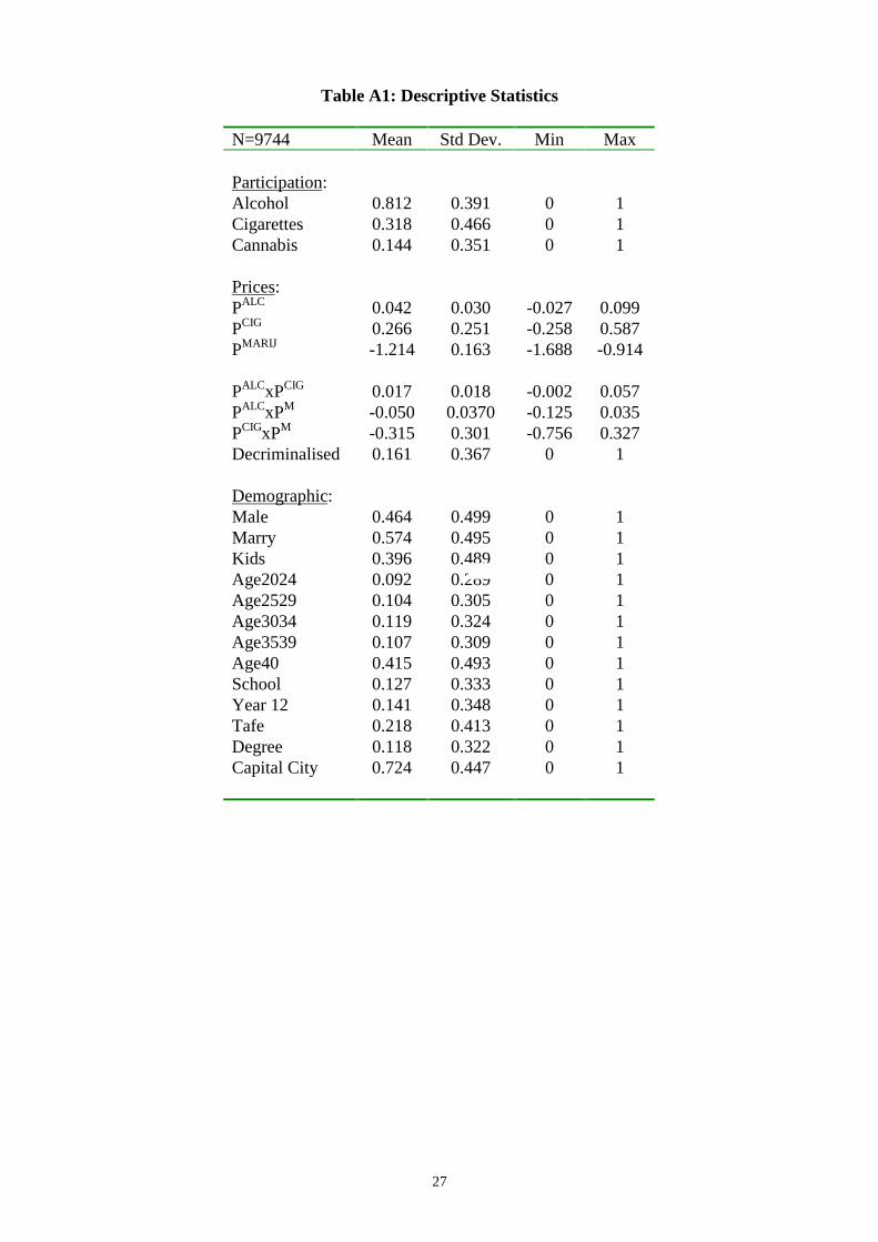
Table A1: Descriptive Statistics

N=9744 Mean Std Dev. Min Max

Participation:Alcohol 0.812 0.391 0 1Cigarettes 0.318 0.466 0 1Cannabis 0.144 0.351 0 1

Prices:PALC 0.042 0.030 -0.027 0.099PCIG 0.266 0.251 -0.258 0.587PMARIJ -1.214 0.163 -1.688 -0.914

PALCxPCIG 0.017 0.018 -0.002 0.057PALCxPM -0.050 0.0370 -0.125 0.035PCIGxPM -0.315 0.301 -0.756 0.327Decriminalised 0.161 0.367 0 1

Demographic:Male 0.464 0.499 0 1Marry 0.574 0.495 0 1Kids 0.396 0.489 0 1Age2024 0.092 0.289 0 1Age2529 0.104 0.305 0 1Age3034 0.119 0.324 0 1Age3539 0.107 0.309 0 1Age40 0.415 0.493 0 1School 0.127 0.333 0 1Year 12 0.141 0.348 0 1Tafe 0.218 0.413 0 1Degree 0.118 0.322 0 1Capital City 0.724 0.447 0 1

28

Table A2: Probit Coefficients corresponding to Table 2.DependentVariable:

Cannabis Alcohol Cigarettes

(1A) (1B) (2) (3)

XF ∂∂ / t-stat XF ∂∂ / t-stat XF ∂∂ / t-stat XF ∂∂ / t-stat

PriceVariables:PMARIJ -0.182 -1.34 -0.264 -1.96* 0.603 3.07* -0.579 -4.14*

PALC 4.84 2.96* 5.01 3.06* -19.48 -2.95* 2.57 1.86

PCIG 0.431 3.06* 0.434 3.08* -2.13 -3.39* 1.32 2.53*

PALC*PCIG -10.61 -3.17* -10.84 -3.22* 12.41 3.78* -5.70 -2.07*

PM*PCIG -0.98 -1.98* 1.25 3.19*

PALC*PM -11.36 -2.22*

Criminal -0.107 -2.04* -0.077 -1.63 0.023 0.54

Crim*PMARIJ 0.078 1.93

Age Categories:20-24 0.178 2.72* 0.178 2.72* 0.102 1.34 0.307 4.88*

25-29 -0.011 -0.16 -0.011 -0.16 0.026 0.33 0.250 3.86*

30-34 -0.268 -3.67* -0.268 -3.67* 0.0009 -0.01 0.177 2.71*

35-39 -0.480 -6.14* -0.480 -6.14* 0.043 0.53 0.111 1.64

40+ -1.284 -18.0* -1.284 -18.0* -0.248 -3.64* -0.237 -4.09*

Male 0.357 10.0* 0.357 10.04* 0.246 7.95* 0.177 6.42*

Married -0.523 -11.9* -0.523 -11.9* 0.020 0.54 -0.326 -9.74*

Kids -0.101 -2.52* -0.101 -2.52* -0.090 -2.58* -0.012 -0.38

At School -0.399 -6.69* -0.399 -6.69* -0.514 -8.11* -0.542 -9.57*

Tafe 0.115 2.38* 0.115 2.37* 0.279 6.76* -0.105 -2.91*

Year 12 0.025 0.50 0.025 0.50 0.284 5.94* -0.182 -4.43*

Degree 0.030 0.49 0.030 0.48 0.456 8.55* -0.443 -9.25*

Capital City 0.093 2.25* 0.093 2.26* -0.004 -0.11 0.039 1.27

Pseudo-R2 0.19 0.19 0.05 0.05N 9744 9744 9744 9744

* - all prices are in logs, the omitted age category is <20 years, the omitted educational category is Year 10.

29

W.A.

S.A.N.S.W.

VIC.

TAS.QLD

Figure 1: Cannabis Participation Rates by State and Year

Proportionof thePopulation

Year