Embed Size (px)
Citation preview
THE REVIEW OF SYMBOLIC LOGIC
Volume 5, Number 1, March 2012
PREFERENCE BASED ON REASONS
DANIEL OSHERSON
Department of Psychology, Princeton University
SCOTT WEINSTEIN
Department of Philosophy, University of Pennsylvania
Abstract. We describe a logic of preference in which modal connectives reflect reasons to desirethat a sentence be true. Various conditions on models are introduced and analyzed.
§1. Introduction. Sometimes preferences are the result of identifiable reasons, aswhen you install a fire alarm for concern about safety. This suggests that studying reasonsalong with preference might illuminate both. An obstacle to such a project is the multitudeof reasons for and against a given action that combine subliminally to yield a decision,as when you go ahead with the fire alarm despite the bother, cost, and false alerts; theunderlying calculus of reason aggregation seems largely hidden from introspection. Thecentrality of reasons to action and rationality is nonetheless sufficient motive to perseverein their analysis despite the difficulty. In this spirit, we here advance a modal logic in whichdifferent reasons for a preference can be aggregated in various ways.
Our inquiry is preceded by several studies of the logic of preference, beginning withvon Wright (1963). More contemporary work includes systems designed to elucidate theinteraction between choice and epistemic possibility (see Lang et al., 2003; van Benthemet al., 2009). Of particular relevance is Liu (2008, chap. 3). This work introduces “prior-ities” (which function like reasons in the present setting) that are ordered by importance,and integrated into a formal language of preference and belief. Several ways of extractingpreferences from priorities are explored. The interplay of preferences and beliefs is alsoanalyzed, along with the impact of updating belief and preference. Liu’s work is closestto the approach taken here inasmuch as it develops a modal language and associatedsemantics. The conceptual framework is nonetheless different from ours, as will becomeclear presently. Another fruitful perspective on the integration of preferences issues fromthe graph-theoretic approach advanced in Andreka et al. (2002); different graphs repre-sent alternative orderings of the alternatives in play, and might be considered separatereasons for choice among them. Within a yet different tradition, multiattribute utility theory(Keeney & Raiffa, 1993) bears directly on reason aggregation through the combination ofutilities based on separate dimensions. The theory has revealed exact conditions underwhich aggregation can proceed additively but it does not explore the logical structure ofreasons and preference, as we shall do here. The insight achievable by formal analysis ofreasons is illustrated by Dietrich & List (2009). These authors demonstrate a representationtheorem relating choice to the respective bundles of reasons that apply to the optionsin play; the axioms needed for their result are remarkably weak. Several issues are thereby
Received: September 17, 2011.
c© Association for Symbolic Logic, 2011
122 doi:10.1017/S1755020311000244
PREFERENCE BASED ON REASONS 123
clarified, among them the significance of combining reasons (their analysis rests not onindividual reasons but on sets of them).
To keep the present project manageable, conceptual issues about the nature of reasonsand their role in rational discourse will be set aside. An entry to this literature is providedby Dietrich & List (2009), and sustained discussion is available in Pettit (2002). Of course,the reasons that come to mind are not necessarily those that govern choice (see, e.g.,Messick, 1985; Haidt, 2001). Our theory is indifferent to this distinction but it will bemore natural to limit examples to conscious effective reasons. The case of the fire alarmserves to convey the character of our theory. Specifically, we picture an agent who imaginesa world that resembles the actual one but with a fire alarm, and another world (possiblyhis own) without one. The agent then compares the two worlds according to various utilityscales (one that measures safety, another cost, and so forth), as well as a distinct utilityscale that takes all the individual scales into account. Our formalism is designed to capturethis picture.
We proceed by first introducing the language under investigation. Informal glosses forsome of its formulas will clarify the ideas in play. Next the semantics of our logic ispresented, followed by consideration of subclasses of models that meet various conditions.We then turn to decidability issues. A discussion of open questions is provided at the end.
§2. Language. The present section introduces a family of modal languages, and dis-cusses the intended meaning of the modality. A language of reason-based preference isdetermined by its signature, which consists of:
(a) a nonempty set P of propositional variables
(b) a nonempty collection S of nonempty subsets of N (the set {0, 1, . . . } of naturalnumbers)
The language of reason-based preference determined by signature (P, S) is denotedL(P, S), and is built from the following symbols.
(a) the set P of propositional variables
(b) the unary connective ¬(c) the binary connective ∧(d) for every set X ∈ S, the binary connective �X
(e) the two parentheses
Formulas are defined inductively via:
p ∈ P | ¬ϕ | (ϕ ∧ ψ) | (ϕ �X ψ) for X ∈ S.
Moreover, we rely on the following abbreviations.
(ϕ ∨ ψ) for ¬(¬ϕ ∧ ¬ψ)
(ϕ → ψ) for (¬ϕ ∨ ψ)
(ϕ ↔ ψ) for ((ϕ → ψ) ∧ (ψ → ϕ))
(ϕ �1...k ψ) for (ϕ �{1...k} ψ)
(ϕ X ψ) for (ϕ �X ψ) ∧ ¬(ψ �X ϕ)
(ϕ ≈X ψ) for (ϕ �X ψ) ∧ (ψ �X ϕ)
124 DANIEL OSHERSON AND SCOTT WEINSTEIN
(ϕ �X ψ) for (ψ �X ϕ)
(ϕ ≺X ψ) for (ψ X ϕ)
for (p → p)
⊥ for ¬ The formula ϕ 1 ψ is to be understood along the following lines. Fix an agent A whosereasoning is at issue. Let u1 be a utility scale that reflects some dimension of interest to A.Then ϕ 1 ψ is true just in case:
A envisions a situation in which ϕ is true and that otherwise differs littlefrom his actual situation (if ϕ is already true then A’s actual situationmay well be the one he envisions). Likewise, A envisions a second sit-uation that is like his actual situation except that ψ is true. Finally, theutility according to u1 of the first imagined situation exceeds that of thesecond.
In the fire alarm example, A envisions his home with a new fire alarm, but with the samefurniture, cat, and fireplace as before. Home with no fire alarm is the actual situation, henceespecially easy to envision. If u1 measures safety, and p is “A will purchase a fire alarm”then p 1 ¬p holds inasmuch as the alarm improves safety. (Since is also true in A’ssituation, p 1 ¬p is materially equivalent to p 1 .) If A is short on cash, and u2reflects finances then p ≺2 ¬p is true, whereas the status of p 1,2 ¬p depends on themanner in which utilities are aggregated (e.g., averaging, minimum, etc.). More generally,we allow preferences ϕ X ψ between arbitrary formulas ϕ,ψ in view of the (possiblymultiple) utilities in X ∈ S. The formula ϕ X ψ thus represents A’s preference for ϕover ψ when A brings to mind just the reasons indexed in X . If
⋃S ∈ S then preference
tout court for ϕ over ψ is represented by ϕ ⋃S ψ , that is, taking account of all reasons
in play.Of course, the greater utility of a given situation compared to another is just one way of
expressing a reason for preferring the former to the latter. More generality can be achievedby representing each kind of reason by an arbitrary binary relation over situations, insteadof insisting on numerical comparisons of cardinal utility. Recourse to such relations willbe raised again in the Discussion section. For now, we develop our theory in the context ofutility, with the expectation that most readers will find this setting conceptually familiar.
If our agent is presumed to be moral then reasons are meant, very roughly, to be good (atleast, not bad ). Morality will here be left unexplored, however. Instead, A is conceived aslogically empowered but otherwise like the rest of us. Also notice how little any of this hasto do with reasons to believe (except for odd cases like being rewarded for reaching genuinereligious conviction). Only reasons for preference will be at issue. There is nonetheless oneconnection to belief that bears comment.
The appeal to situations that differ minimally from the actual one, except for satisfy-ing a given formula, is familiar from well-known theories of counterfactual conditionals(Stalnaker, 1968; Lewis, 1973). It thus risks bedevilment from a similar range of cases.Suppose, for example, that p is “Winter ends a little earlier than last year.” Then toomany p-worlds offer themselves as alternatives to the actual world (since the set of shorterwinters has no member closest to last year’s winter). The present endeavor, however, maynot be as vulnerable as the earlier one to such cases. For it here suffices that the reasoningagent bring to mind a cognitively salient situation that satisfies the formula in question(e.g., winter a week shorter), not necessarily the maximally similar one. Indeed, the agent

PREFERENCE BASED ON REASONS 125
may not be prepared to identify the maximally similar p-world, or even to understandsuch an idea. Consistent with this relaxed attitude, to each consistent proposition oursemantics assigns a world that represents life were the proposition true, where the choiceof world may depend on the agent’s current position. Some constraints on the choice willbe examined, but otherwise the reasoning agent is on his own. We take all this to be arough idealization of what happens in actual decision making. One imagines an alternativesituation that satisfies the proposition at issue, then evaluates it along various dimensions(i.e., utility scales).
The utility scales that determine the truth of modal formulas are intended to measurethe impact on choice of specific considerations, for example, cost, health, professionaladvancement. Because deliberation is assumed to transpire in a single mind (the agent’s),aggregation of different scales into an overall value seems feasible; indeed, people do itall the time. For simplicity, the scales express expected utilities, that is, with probabilitiesalready factored in. Thus, the safety improvements envisioned from installing a fire alarmalready integrate the agent’s confidence that the device will work as advertised.
Even when utility scales are kept separate, languages of reason-based preference allowinteresting interactions. For an illustration, first observe that ϕ i means (roughly) thatthe ui -utility of the envisioned ϕ-world exceeds that of the actual world. Now consider:
(p 1 ) 2 .
This says that the agent has a u2-reason for there being a u1-reason in favor of p. Forexample, let p be the assertion that you buy a low-power automobile. Let u2-utility bepecuniary: u2(w1) > u2(w2) iff you have more cash in w1 compared to w2. Let u1-utilityreflect personal safety: u1(w1) > u1(w2) iff you incur less risk traveling in w1 than in w2.Then the formula asserts that it’s in your financial interest that your buying a low-powerautomobile is in your safety interest—which might well be true inasmuch as low-powervehicles are cheaper.
We conclude this section with another illustration of the interaction of individual utilityscales. Consider:
¬q 1 (p 2 q).
This says that the agent u1-prefers that q be false rather than u2-prefer p over q. Forexample, let q be the assertion that your brother runs for mayor, and let p be that MissSmith (no relation) also runs. Let u1-utility measure family pride, and let u2-utility measurepolitical value to an ailing municipality. Then the formula asserts that from the point ofview of family pride, you’d rather that your brother not run for mayor than that Miss Smithbe the superior candidate.
§3. Semantics. We now provide a formal semantics designed to capture the intu-itive picture elaborated in the preceding section. Several preliminary concepts are needed.Fundamental is the choice of a nonempty set W to embody the imaginative possibilities(“worlds”) available to an agent in the course of practical deliberation. Subsets of W arecalled propositions. As discussed above, given a nonempty proposition A and a world w,an agent envisions a salient alternative to w among the worlds in A. (If w ∈ A then the“alternative” might be w itself.) We formalize this idea as follows.
DEFINITION 3.1. A selection function s overW is a mapping fromW×{A ⊆ W | A �= ∅}to W such that for all w ∈ W and ∅ �= A ⊆ W, s(w, A) ∈ A.
126 DANIEL OSHERSON AND SCOTT WEINSTEIN
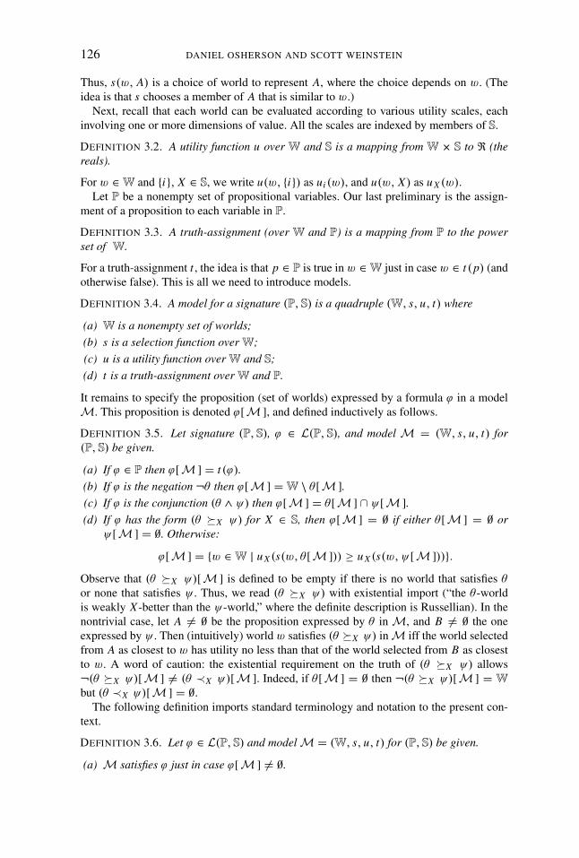
Thus, s(w, A) is a choice of world to represent A, where the choice depends on w. (Theidea is that s chooses a member of A that is similar to w.)
Next, recall that each world can be evaluated according to various utility scales, eachinvolving one or more dimensions of value. All the scales are indexed by members of S.
DEFINITION 3.2. A utility function u over W and S is a mapping from W × S to � (thereals).
For w ∈ W and {i}, X ∈ S, we write u(w, {i}) as ui (w), and u(w, X) as u X (w).Let P be a nonempty set of propositional variables. Our last preliminary is the assign-
ment of a proposition to each variable in P.
DEFINITION 3.3. A truth-assignment (over W and P) is a mapping from P to the powerset of W.
For a truth-assignment t , the idea is that p ∈ P is true in w ∈ W just in case w ∈ t (p) (andotherwise false). This is all we need to introduce models.
DEFINITION 3.4. A model for a signature (P, S) is a quadruple (W, s, u, t) where
(a) W is a nonempty set of worlds;
(b) s is a selection function overW;
(c) u is a utility function over W and S;
(d) t is a truth-assignment over W and P.
It remains to specify the proposition (set of worlds) expressed by a formula ϕ in a modelM. This proposition is denoted ϕ[M ], and defined inductively as follows.
DEFINITION 3.5. Let signature (P, S), ϕ ∈ L(P, S), and model M = (W, s, u, t) for(P, S) be given.
(a) If ϕ ∈ P then ϕ[M ] = t (ϕ).
(b) If ϕ is the negation ¬θ then ϕ[M ] = W \ θ [M ].
(c) If ϕ is the conjunction (θ ∧ ψ) then ϕ[M ] = θ [M ] ∩ ψ[M ].
(d) If ϕ has the form (θ �X ψ) for X ∈ S, then ϕ[M ] = ∅ if either θ [M ] = ∅ orψ[M ] = ∅. Otherwise:
ϕ[M ] = {w ∈ W | u X (s(w, θ [M ])) ≥ u X (s(w,ψ[M ]))}.Observe that (θ �X ψ)[M ] is defined to be empty if there is no world that satisfies θor none that satisfies ψ . Thus, we read (θ �X ψ) with existential import (“the θ -worldis weakly X -better than the ψ-world,” where the definite description is Russellian). In thenontrivial case, let A �= ∅ be the proposition expressed by θ in M, and B �= ∅ the oneexpressed by ψ . Then (intuitively) world w satisfies (θ �X ψ) inM iff the world selectedfrom A as closest to w has utility no less than that of the world selected from B as closestto w. A word of caution: the existential requirement on the truth of (θ �X ψ) allows¬(θ �X ψ)[M ] �= (θ ≺X ψ)[M ]. Indeed, if θ [M ] = ∅ then ¬(θ �X ψ)[M ] = W
but (θ ≺X ψ)[M ] = ∅.The following definition imports standard terminology and notation to the present con-
text.
DEFINITION 3.6. Let ϕ ∈ L(P, S) and modelM = (W, s, u, t) for (P, S) be given.
(a) M satisfies ϕ just in case ϕ[M ] �= ∅.
PREFERENCE BASED ON REASONS 127
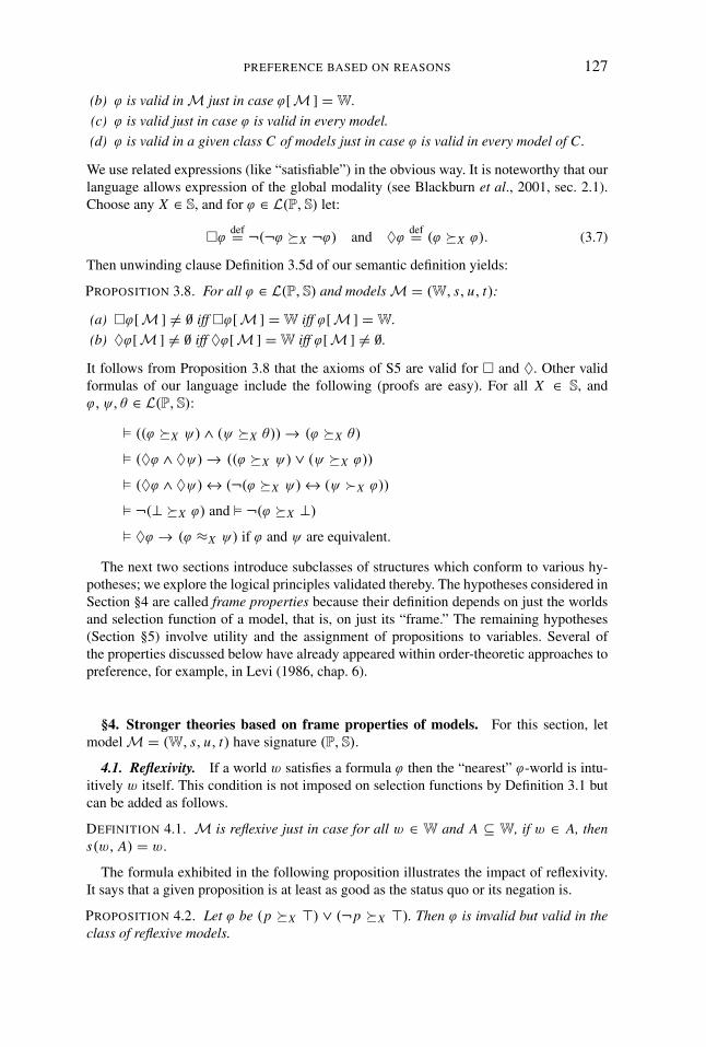
(b) ϕ is valid inM just in case ϕ[M ] = W.
(c) ϕ is valid just in case ϕ is valid in every model.
(d) ϕ is valid in a given class C of models just in case ϕ is valid in every model of C.
We use related expressions (like “satisfiable”) in the obvious way. It is noteworthy that ourlanguage allows expression of the global modality (see Blackburn et al., 2001, sec. 2.1).Choose any X ∈ S, and for ϕ ∈ L(P, S) let:
�ϕdef= ¬(¬ϕ �X ¬ϕ) and ♦ϕ
def= (ϕ �X ϕ). (3.7)
Then unwinding clause Definition 3.5d of our semantic definition yields:
PROPOSITION 3.8. For all ϕ ∈ L(P, S) and modelsM = (W, s, u, t):
(a) �ϕ[M ] �= ∅ iff �ϕ[M ] = W iff ϕ[M ] = W.
(b) ♦ϕ[M ] �= ∅ iff ♦ϕ[M ] = W iff ϕ[M ] �= ∅.
It follows from Proposition 3.8 that the axioms of S5 are valid for � and ♦. Other validformulas of our language include the following (proofs are easy). For all X ∈ S, andϕ,ψ, θ ∈ L(P, S):
� ((ϕ �X ψ) ∧ (ψ �X θ)) → (ϕ �X θ)
� (♦ϕ ∧ ♦ψ) → ((ϕ �X ψ) ∨ (ψ �X ϕ))
� (♦ϕ ∧ ♦ψ) ↔ (¬(ϕ �X ψ) ↔ (ψ X ϕ))
� ¬(⊥ �X ϕ) and � ¬(ϕ �X ⊥)
� ♦ϕ → (ϕ ≈X ψ) if ϕ and ψ are equivalent.
The next two sections introduce subclasses of structures which conform to various hy-potheses; we explore the logical principles validated thereby. The hypotheses considered inSection §4 are called frame properties because their definition depends on just the worldsand selection function of a model, that is, on just its “frame.” The remaining hypotheses(Section §5) involve utility and the assignment of propositions to variables. Several ofthe properties discussed below have already appeared within order-theoretic approaches topreference, for example, in Levi (1986, chap. 6).
§4. Stronger theories based on frame properties of models. For this section, letmodelM = (W, s, u, t) have signature (P, S).
4.1. Reflexivity. If a world w satisfies a formula ϕ then the “nearest” ϕ-world is intu-itively w itself. This condition is not imposed on selection functions by Definition 3.1 butcan be added as follows.
DEFINITION 4.1. M is reflexive just in case for all w ∈ W and A ⊆ W, if w ∈ A, thens(w, A) = w.
The formula exhibited in the following proposition illustrates the impact of reflexivity.It says that a given proposition is at least as good as the status quo or its negation is.
PROPOSITION 4.2. Let ϕ be (p �X ) ∨ (¬p �X ). Then ϕ is invalid but valid in theclass of reflexive models.

128 DANIEL OSHERSON AND SCOTT WEINSTEIN
Proof. To verify the invalidity of ϕ, suppose that W = {w0, w1, w2}, t (p) = {w0, w1},s(w0, {w0, w1}) = s(w0, p[M ]) = w1, s(w0, {w2}) = s(w0, ¬p[M ]) = w2,s(w0,W) = s(w0, [M ]) = w0, and u X (w0) > u X (w1), u X (w2). Then it is easy tosee that w0 �∈ ϕ[M ] hence ϕ is not valid.
On the other hand, suppose that M is reflexive, and let w0 ∈ W. Then either w0 ∈p[M ] or w0 ∈ ¬p[M ], say the former (the other case is parallel). By reflexivity,s(w0, p[M ] = w0. Likewise, w0 ∈ [M ] = W, so again by reflexivity, s(w0, [M ] =w0. Since u X (w0) ≥ u X (w0), w0 ∈ ϕ[M ]. �
Reflexivity entails that some formulas are satisfied only by infinite models.
PROPOSITION 4.3. There is ϕ ∈ L(P, S) such that ϕ is satisfied by some infinite reflexivemodel but by no finite reflexive model.
Proof. Let ϕ be the conjunction of the following formulas.
(4.4) (a) �(p → (p ≺X ¬p))
(b) �(¬p → (¬p ≺X p))
It is easy to verify that ϕ is satisfied by a model whose worlds form an ω-sequencewhen ordered by u X , and which alternate between satisfying p and ¬p. On the other hand,suppose for a contradiction that ϕ is satisfied by finite model M = (W, s, u, t). Thensome w0 ∈ W has maximum u X utility. Suppose that w0 satisfies p (the other case isparallel). Then (4.4)a and Reflexivity imply that there is w1 ∈ W satisfying ¬p such thatu X (w0) < u X (w1). This contradicts the choice of w0 as having maximum u X utility. �
4.2. Regularity. If you think that living in Boston is most similar to your currentsituation among the set of all addresses in New England then shouldn’t you think thatliving in Boston is most similar to your current situation among the set of all addressesin Massachusetts? A similar principle is standardly applied to choice (Sen, 1971) eventhough its violation has been documented in several empirical studies (e.g., Payne & Puto,1982; Tentori et al., 2001). In the present setting, we are led to the following constraint onselection.
DEFINITION 4.5. M is regular just in case for all w ∈ W, nonempty A ⊆ B ⊆ W, andw1 ∈ A: If s(w, B) = w1 then s(w, A) = w1.
Regularity validates the formula appearing in the next proposition. An instance is this: Ifbuying either a Ford or a Chevy makes more sense than buying a Toyota then either itmakes more sense to buy a Ford than a Toyota, or it makes more sense to buy a Chevy thana Toyota (or both).
PROPOSITION 4.6. Let ϕ be ((p ∨ q) X r) → ((p X r) ∨ (q X r)). Then ϕ is invalidbut valid in the class of regular models.
Proof. A countermodel for ϕ is easy to devise. To show validity in the regular models,suppose that M is regular, and let w ∈ ((p ∨ q) X r)[M ] be given. Then there arew1, w2 ∈ W with:
(4.7) (a) w1 = s(w, (p ∨ q)[M ]),
(b) w2 = s(w, r [M ]), and
(c) u X (w1) > u X (w2).
PREFERENCE BASED ON REASONS 129
By (4.7)a, either w1 ∈ t (p) or w1 ∈ t (q), say the latter (the other case is parallel). Sinceq[M ] ⊆ (p ∨ q)[M ], it follows from regularity that w1 = s(w, q[M ]). In view of(4.7)b and c, w ∈ (q X r)[M ]. �
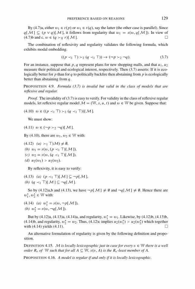
The combination of reflexivity and regularity validates the following formula, whichexhibits modal embedding.
((p ≺1 ) 2 (q ≺1 )) → (¬p 2 ¬q). (3.7)
For an instance, suppose that p, q represent plans for new shopping malls, and that u1, u2measure their political and ecological interest, respectively. Then (3.7) asserts: If it is eco-logically better for p than for q to politically backfire then abstaining from p is ecologicallybetter than abstaining from q.
PROPOSITION 4.9. Formula (3.7) is invalid but valid in the class of models that arereflexive and regular.
Proof. The invalidity of (3.7) is easy to verify. For validity in the class of reflexive regularmodels, let reflexive regular modelM = (W, s, u, t) and w ∈ W be given. Suppose that:
(4.10) w ∈ ((p ≺1 ) 2 (q ≺1 ))[M ].
We must show:
(4.11) w ∈ (¬p 2 ¬q)[M ].
By (4.10), there are w1, w2 ∈ W with:
(4.12) (a) 1 )M) �= ∅,
(b) w1 = s(w, (p ≺1 )[M ]),
(c) w2 = s(w, (q ≺1 )[M ]),
(d) u2(w1) > u2(w2).
By reflexivity, it is easy to verify:
(4.13) (a) (p ≺1 )[M ] ⊆ ¬p[M ],
(b) (q ≺1 )[M ] ⊆ ¬q[M ].
So by (4.12)a,b and (4.13), we have ¬p[M ] �= ∅ and ¬q[M ] �= ∅. Hence there arew∗
1, w∗2 ∈ W with:
(4.14) (a) w∗1 = s(w, ¬p[M ]),
(b) w∗2 = s(w, ¬q[M ]).
But by (4.12)a, (4.13)a, (4.14)a, and regularity, w∗1 = w1. Likewise, by (4.12)b, (4.13)b,
(4.14)b, and regularity, w∗2 = w2. Thus, (4.12)c implies u2(w
∗1) > u2(w
∗2) which together
with (4.14) yields (4.11). �An alternative formulation of regularity is given by the following definition and propo-
sition.
DEFINITION 4.15. M is locally lexicographic just in case for every v ∈ W there is a wellorder Rv of W such that for all A ⊆ W, s(v, A) is the Rv -least member of A.
PROPOSITION 4.16. A model is regular if and only if it is locally lexicographic.
130 DANIEL OSHERSON AND SCOTT WEINSTEIN
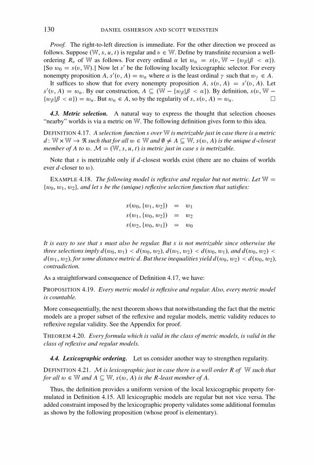
Proof. The right-to-left direction is immediate. For the other direction we proceed asfollows. Suppose (W, s, u, t) is regular and v ∈ W. Define by transfinite recursion a well-ordering Rv of W as follows. For every ordinal α let wα = s(v,W − {wβ |β < α}).[So w0 = s(v,W).] Now let s′ be the following locally lexicographic selector. For everynonempty proposition A, s′(v, A) = wα where α is the least ordinal γ such that wγ ∈ A.
It suffices to show that for every nonempty proposition A, s(v, A) = s′(v, A). Lets′(v, A) = wα . By our construction, A ⊆ (W − {wβ |β < α}). By definition, s(v,W −{wβ |β < α}) = wα . But wα ∈ A, so by the regularity of s, s(v, A) = wα . �
4.3. Metric selection. A natural way to express the thought that selection chooses“nearby” worlds is via a metric on W. The following definition gives form to this idea.
DEFINITION 4.17. A selection function s overW is metrizable just in case there is a metricd : W×W → � such that for all w ∈ W and ∅ �= A ⊆ W, s(w, A) is the unique d-closestmember of A to w.M = (W, s, u, t) is metric just in case s is metrizable.
Note that s is metrizable only if d-closest worlds exist (there are no chains of worldsever d-closer to w).
EXAMPLE 4.18. The following model is reflexive and regular but not metric. Let W ={w0, w1, w2}, and let s be the (unique) reflexive selection function that satisfies:
s(w0, {w1, w2}) = w1
s(w1, {w0, w2}) = w2
s(w2, {w0, w1}) = w0
It is easy to see that s must also be regular. But s is not metrizable since otherwise thethree selections imply d(w0, w1) < d(w0, w2), d(w1, w2) < d(w0, w1), and d(w0, w2) <d(w1, w2), for some distance metric d. But these inequalities yield d(w0, w2) < d(w0, w2),contradiction.
As a straightforward consequence of Definition 4.17, we have:
PROPOSITION 4.19. Every metric model is reflexive and regular. Also, every metric modelis countable.
More consequentially, the next theorem shows that notwithstanding the fact that the metricmodels are a proper subset of the reflexive and regular models, metric validity reduces toreflexive regular validity. See the Appendix for proof.
THEOREM 4.20. Every formula which is valid in the class of metric models, is valid in theclass of reflexive and regular models.
4.4. Lexicographic ordering. Let us consider another way to strengthen regularity.
DEFINITION 4.21. M is lexicographic just in case there is a well order R of W such thatfor all w ∈ W and A ⊆ W, s(w, A) is the R-least member of A.
Thus, the definition provides a uniform version of the local lexicographic property for-mulated in Definition 4.15. All lexicographic models are regular but not vice versa. Theadded constraint imposed by the lexicographic property validates some additional formulasas shown by the following proposition (whose proof is elementary).
PREFERENCE BASED ON REASONS 131
PROPOSITION 4.22. Let ϕ be (p �X q) → �(p �X q). Then ϕ is false in some regularmodel but valid in the class of lexicographic models.
A natural generalization of lexicographic ordering may be defined as follows.
DEFINITION 4.23. A selection function s over W is proposition driven just in case for allw1, w2 ∈ W and ∅ �= A ⊆ W, s(w1, A) = s(w2, A).
That is, proposition driven selection functions ignore their first arguments. Lexicographicordering implies proposition drivenness; the next proposition shows the former to be astronger condition than the latter.
PROPOSITION 4.24. There is a formula satisfiable in the class of proposition driven modelsbut not in the class of lexicographic models.
Proof. Let ϕ be the conjunction of the following formulas.
(p ∨ q) X p ≺X q ≺X .
It is easy to verify that no regular model satisfies ϕ but that some proposition drivenmodel does. Since lexicographic ordering implies regularity, the proposition follows im-mediately. �
The next proposition is a corollary to Proposition 4.16.
PROPOSITION 4.25. A model is proposition driven and regular if and only if it is lexico-graphic.
§5. Stronger theories that are not based on frames. We now consider propertiesof models that cannot be defined just in terms of (W, s), the frame of a model. Thebackground signature (P, S) may thus be expected to interact with the validity of formulasin classes of models specified by these properties.
5.1. Proximity. Intuitively, a selection function applied to a world w and nonemptyproposition A should pick a member w1 of A that is “near” or “similar” to w. One wayto articulate this idea is to require that the two worlds differ minimally in the sets ofpropositional variables that each makes true. The following notation helps us formulatethis idea. For w ∈ W, let t−1(w) = {p ∈ P | w ∈ t (p)}. That is, t−1(w) is the setof propositional variables that M satisfies at w. For sets S, T , let S � T denote theirsymmetric difference (S \ T ) ∪ (T \ S). Then the idea of selecting “nearby worlds” can berendered as follows.
DEFINITION 5.1. M is proximal just in case the following condition is met, for all w ∈ Wand all nonempty propositions A ⊆ W.
If s(w, A) = w1 then there is no w2 ∈ A such that t−1(w) � t−1(w2) ⊂ t−1(w) �t−1(w1).
For example, suppose that t−1(w) = {p, q}, t−1(w1) = {p, r}, and t−1(w2) = {p, q, r}.Let A = {w1, w2}. Then s violates proximity if s(w, A) = w1 since t−1(w) � t−1(w2) ={r} ⊂ {q, r} = t−1(w) � t−1(w1).
For the next two propositions, we rely on an hypothesis about our signature, namely, thatP = {p, q, r}. In conjunction with regularity, proximity validates a formula reminiscent ofthe sure thing principle (Savage, 1954).
132 DANIEL OSHERSON AND SCOTT WEINSTEIN
PROPOSITION 5.2. Let ϕ be
(((p ∧ r) X (q ∧ r)) ∧ ((p ∧ ¬r) X (q ∧ ¬r))) → (p X q).
Then ϕ is invalid in the class of regular and in the class of proximal models but valid in theclass of models that are both regular and proximal.
An instance of ϕ is the following. If one has better reason to vacation in Florence during anItalian transport strike than to vacation in Rome during such a transport strike, and if onehas better reason to vacation in Florence with no transport strike than to vacation in Romewith no such strike then one has better reason to vacation in Florence than in Rome.
Proof of Proposition 5.2. Construction of the needed countermodels is left for the reader.Suppose thatM is regular and proximal with w ∈ W. Either w ∈ t (r) or w �∈ t (r); assumethe former (the argument is parallel in the other case). There is nothing left to prove unlessthe following statements are true [since otherwise the left conjunct in the antecedent of ϕis false; see Definition 3.5d].
(5.3) (a) t (p) ∩ t (r) �= ∅(b) t (q) ∩ t (r) �= ∅.
By (5.3), p[M ] �= ∅ and q[M ] �= ∅. So let w1, w2 ∈ W be such that:
(5.4) (a) w1 = s(w, p[M ])
(b) w2 = s(w, q[M ]).
Since w ∈ t (r), (5.3)a, (5.4)a, and proximity imply w1 ∈ t (p) ∩ t (r). Hence, w1 ∈(p ∧ r)[M ] ⊆ p[M ], so regularity implies w1 = s(w, (p ∧ r)[M ]). Likewise, w2 =s(w, (q ∧ r)[M ]). From (p ∧ r) X (q ∧ r) we infer u X (w1) > u X (w2) which in viewof (5.4) implies p X q. Thus w ∈ ϕ[M ]. �
Similar reasoning suffices to prove:
PROPOSITION 5.5. Let ϕ be
(p ∧ ((p ∧ q) X r)) → (q X r).
Then ϕ is invalid in the class of regular and in the class of proximal models but valid in theclass of models that are both regular and proximal.
For an instance of this formula, suppose that you have a greater gustatory interest inham and eggs than just oatmeal. Then if you already have ham, you’ll be more interestedin eggs than just oatmeal.
5.2. Extensionality, saturation, and perfection. We next consider the relation betweenworlds and the propositional variables they satisfy. The following condition requires thatdistinct worlds don’t make the same variables true.
DEFINITION 5.6. M is extensional just in case for all w1, w2 ∈ W, {v ∈ P | w1 ∈ t (v)} ={v ∈ P | w2 ∈ t (v)} implies w1 = w2.
Observe that if P is finite then every extensional model is finite. Also, it is easy to see thatevery proximal extensional model is reflexive. Hence, in a finite signature, no such modelsatisfies the conjunction of Formulas (4.4)(a) and (b). If P = {p} then obviously the invalidformula (p ≈X ¬p) → (p ≈X ) is valid in the extensional models.
If every subset of variables inhabits some world, the model may be called “saturated.”
PREFERENCE BASED ON REASONS 133
DEFINITION 5.7. M is saturated just in case for all T ⊆ P there is w ∈ W with {v ∈ P |w ∈ t (v)} = T .
DEFINITION 5.8. M is perfect just in caseM is both extensional and saturated.
In a perfect model, W can be identified with the power set of P. The combination ofperfection and proximity has consequences for the “contraposition” of reasons, as in (p X
q) → (¬q X ¬p). This formula is plausible at first sight; for it seems that if p is u X -superior to q then u X also favors q rather than p failing to hold. Thus, keeping a promiseis morally superior to teasing the infirm hence not teasing the infirm should be morallysuperior to not keeping a promise, which it is. Closer inspection, however, reveals thatonly a weaker form of contraposition can be maintained.
PROPOSITION 5.9. Let C be the class of perfect and proximal models. Then (p X q) →(¬q X ¬p) is not valid in C. However, ((¬p ∧ ¬q) → (p X q)) is valid in a givenmodel of C iff ((p ∧ q) → (¬q X ¬p)) is valid in the same model.
Proof. We demonstrate the left-to-right direction in the second part of the proposition.LetM ∈ C be given, and suppose that:
(5.10) (¬p ∧ ¬q) → (p X q) is valid inM.
By saturation, let w ∈ t (p) ∩ t (q). By saturation again, there are w1, w2 ∈ W with:
(5.11) (a) w1 = s(w, ¬q[M ]), and
(b) w2 = s(w, ¬p[M ]).
To complete the proof it suffices to show that:
(5.12) u X (w1) > u X (w2).
By (5.11), proximity, and perfection:
(5.13) (a) w1 satisfies the same variables as w, except for q.
(b) w2 satisfies the same variables as w, except for p.
By perfection, there is w∗ ∈ W that satisfies the same subset of P as w except for p, q.That is, w∗ falsifies p and q but otherwise agrees with w. Hence by (5.10), w∗ ∈ (p X
q)[M ]. So there are w′1, w
′2 ∈ W with:
(5.14) (a) w′1 = s(w∗, p[M ]),
(b) w′2 = s(w∗, q[M ]), and
(c) u X (w′1) > u X (w′
2).
By (5.14)a,b, proximity, and perfection:
(5.15) (a) w′1 satisfies the same variables as w∗, except for p.
(b) w′2 satisfies the same variables as w∗, except for q.
From (5.13), (5.15), and perfection, w1 = w′1 and w2 = w′
2. Therefore, (5.12) followsfrom (5.14)c. �
134 DANIEL OSHERSON AND SCOTT WEINSTEIN
5.3. Conditions on the utility function. We now consider different ways that utilitiescan be combined. This topic is at the heart of the relation between reasons and preference.For as noted earlier, we conceive preference for ϕ over ψ to be represented by ϕ ⋃
S ψ ,that is, taking account of all reasons in play. (Here it is assumed that
⋃S ∈ S.) We start
with the most basic condition on utility aggregation, namely, that u X depends on just theui indexed by X .
DEFINITION 5.16. Let finite X ∈ S be given. ModelM is local for X just in case:
(a) for all i ∈ X, {i} ∈ S and
(b) there is a function g from finite subsets of � to � such that for all w ∈ W, u X (w) =g(〈ui (w) | i ∈ X〉).
In this case, we call ϕ ∈ L(P, S) g-valid if ϕ is true in the class of models for which u X iscomputed via g.
For example, locality prevents u{1,2}(w) from depending on u3(w). It is easy to seethat the following formula is valid in the class of {1, 2}-local models but false in somenon{1, 2}-local model.
((p ≈1 p′) ∧ (q ≈1 q ′) ∧ (p ≈2 p′) ∧ (q ≈2 q ′)) → ((p ≈{1,2} q) ↔ (p′ ≈{1,2} q ′)).
Candidates for g in Definition 5.16 include:
u X (w) =average{ui (w) | i ∈ X} median{ui (w) | i ∈ X}
minimum{ui (w) | i ∈ X} maximum{ui (w) | i ∈ X}
Formulas separate some of these locality classes. For example, the following schema isaverage-valid but neither min- nor max-valid with respect to {i, j}.
((ϕ i ψ) ∧ (ϕ ≈ j ψ)) → (ϕ {i, j} ψ).
To see that the schema is not min-valid, take u j to assign identical numbers to all worlds,much smaller than the numbers that ui assigns. Do the reverse for a countermodel to max-validity.
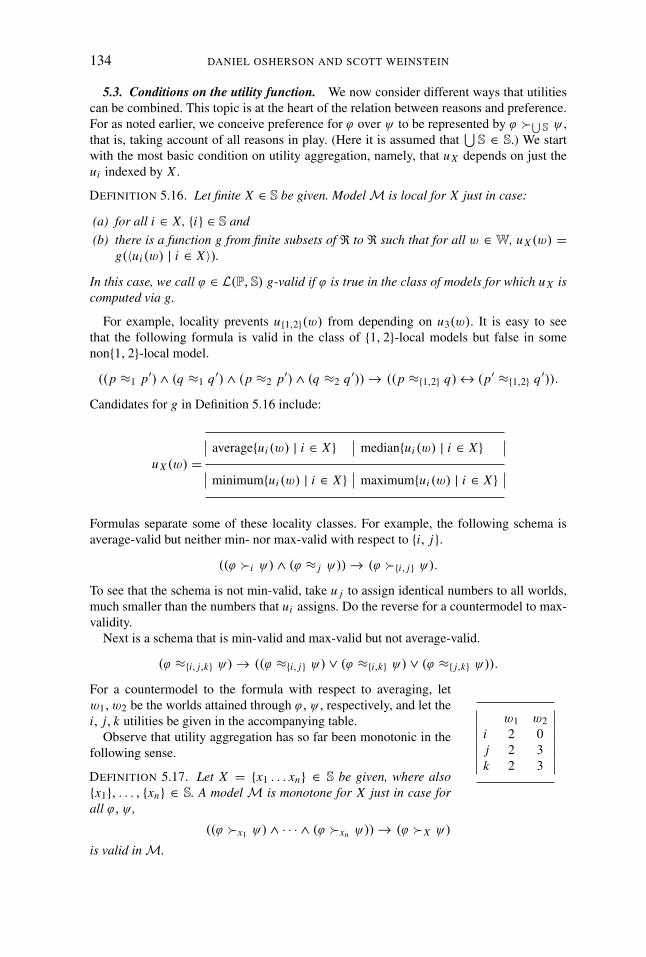
Next is a schema that is min-valid and max-valid but not average-valid.
(ϕ ≈{i, j,k} ψ) → ((ϕ ≈{i, j} ψ) ∨ (ϕ ≈{i,k} ψ) ∨ (ϕ ≈{j,k} ψ)).
w1 w2i 2 0j 2 3k 2 3
For a countermodel to the formula with respect to averaging, letw1, w2 be the worlds attained through ϕ,ψ , respectively, and let thei, j, k utilities be given in the accompanying table.
Observe that utility aggregation has so far been monotonic in thefollowing sense.
DEFINITION 5.17. Let X = {x1 . . . xn} ∈ S be given, where also{x1}, . . . , {xn} ∈ S. A modelM is monotone for X just in case forall ϕ,ψ ,
((ϕ x1 ψ) ∧ · · · ∧ (ϕ xn ψ)) → (ϕ X ψ)
is valid inM.
PREFERENCE BASED ON REASONS 135
The four functions discussed above are consistent with monotonicity but it is easy toimagine circumstances in which nonmonotonic aggregation takes place. For example, youmight prefer to spend time with people of luxuriant life style (they’re more fun), encodedin u1, and also prefer people who espouse asceticism and self-restraint (they’re moreadmirable), encoded in u2. The two utility functions considered individually might orderJim above Jack as dinner partners but u1,2 will reverse the preference if it is sensitive toJim’s hypocrisy.
§6. Decidability and compactness. The present section offers three theorems aboutthe compactness and decidability of satisfiability (hence, about the decidability of validityas well). For this purpose, we fix a signature (P, S) in which P is an initial segment of N,and S is a set of finite subsets of N. The first theorem concerns satisfiability with respect tothe class of all models.
THEOREM 6.1. The set of satisfiable formulas of L(P, S) is decidable.
Adjustments to the proof of Theorem 6.1 verify the following corollaries.
COROLLARY 6.2. If a formula of L(P, S) is satisfiable then it is satisfied in a finite model(i.e., in a model with finitely many worlds).
COROLLARY 6.3. The set of formulas ofL(P, S) that are satisfiable in the class of reflexivemodels is decidable.
Corollary 6.2 may be contrasted with Proposition 4.3, stating that some formulas can besatisfied by a reflexive model only if the model contains infinitely many worlds.
The second theorem bears on lexicographic ordering in the sense of Definition 4.21, andon proposition drivenness in the sense of Definition 4.23.
THEOREM 6.4. The set of formulas of L(P, S) that are satisfiable in the class of lexico-graphic models is decidable, as is the set of formulas that are satisfiable in the class ofproposition driven models. Indeed, both sets of formulas are NP-complete.
The final theorem affirms that satisfiability with respect to the class of all models iscountably compact. We call a collection ⊆ L of formulas “satisfiable” just in case thereis a modelM that satisfies every member of at a common point, that is, just in case:⋂
{ϕ[M ] | ϕ ∈ } �= ∅.
THEOREM 6.5. Suppose that signature (P, S) is countable, and let ⊆ L(P, S) be given.Then is satisfiable if and only if every finite subset of is satisfiable.
On the other hand, if either P or S is uncountable then compactness breaks down. Proofsof the theorems are provided in the Appendix.
§7. Generalized frames. In our theory, ϕ �X ψ can be understood as asserting thatu X assigns at least as much value to the proposition expressed by ϕ as to the propositionexpressed by ψ . The latter two propositions are represented by elements of each, pickedout as a function of the world at which the formula is evaluated. A natural generalizationis to compare the value of propositions directly, without recourse to individual worlds asrepresentatives. We explore this idea in the present section. Let (P, S) be our background
136 DANIEL OSHERSON AND SCOTT WEINSTEIN
signature, and recall that a total preorder is transitive, connected, and reflexive over itsdomain.
DEFINITION 7.1. Let a set W of worlds be given.
(a) By a value-ordering for W and S is meant a function v from W × S to the set oftotal preorders over the class of nonempty subsets of W. We call the pair (W, v) ageneralized frame.
(b) Let a truth-assignment t and a value-ordering v forW and S be given. Then (W, t, v)is a generalized model.
Intuitively, a value-ordering arranges propositions by utility, relative to index X ∈ S andvantage point w ∈ W. The semantics of generalized models is given by Definition 3.5with the following substitution for Clause 3.5d. Let ϕ ∈ L(P, S) and generalized modelM = (W, t, v) for (P, S) be given.
3.5d′ If ϕ has the form (θ �X ψ) for X ∈ S, then ϕ[M ] = ∅ if eitherθ [M ] = ∅ or ψ[M ] = ∅. Otherwise:
ϕ[M ] = {w ∈ W | θ [M ] comes no earlier than ψ[M ] in v(w, X)}.
Now let modelM = (W, s, u, t) be given. Then a value-ordering v is induced by thefollowing condition. For w ∈ W, X ∈ S, and nonempty A, B ⊆ W, A is (weakly) orderedafter B iff u X (wA) ≥ u X (wB) where wA = s(w, A) and wB = s(w, B). (The truth-assignment t plays no role.) We call (W, v) the generalized frame induced byM.
Given a model (W, s, u, t), w ∈ W, and nonempty A ⊆ W, there is w0 ∈ W withu X (s(w, A)) = u X (s(w, {w0})), namely, w0 = s(w, A). So we have:
LEMMA 7.2. Let value-ordering v be induced by model (W, s, u, t). Then for all w ∈ Wand X ∈ S, every equivalence class in v(w, X) contains a singleton set.
We have the following immediate consequence, which shows that some generalized framescannot be induced by models.
PROPOSITION 7.3. Let W contain at least two worlds. Let value-ordering v be such thatfor some w ∈ W and X ∈ S, either
(a) v(w, X) refines ⊂ over the field of nonempty subsets of W or
(b) v(w, X) is a strict linear order over the nonempty subsets of W.
Then (W, v) is not induced by any model.
On the other hand, the next proposition shows that some interesting classes of generalizedframes can be characterized in L(P, S). We say that ϕ ∈ L(P, S) is valid in a generalizedframe (W, v) in case ϕ is true in every generalized model of form (W, t, v).
PROPOSITION 7.4. Let X ∈ S be given. There are ϕ1, ϕ2 ∈ L(P, S) such that
(a) ϕ1 is valid in a generalized frame (W, v) if and only if for all w ∈ W, v(w, X) refines⊂ over the nonempty subsets of W;
(b) ϕ2 is valid in a generalized frame (W, v) if and only if for all w ∈ W, v(w, X) is astrict linear order over the nonempty subsets of W.
Proof. It is easy to verify the proposition with the following choices of ϕ1, ϕ2, respec-tively.
PREFERENCE BASED ON REASONS 137
(�(p → q) ∧ ¬�(q → p) ∧ ♦p) → p ≺X q
¬�(p ↔ q) → ((p ≺X q) ∨ (q ≺X p))
�In Osherson & Weinstein (To appear), we provide an axiomatization of the set of formu-
las that are valid in generalized frames and establish that a formula is valid in the class ofgeneralized frames if and only if it is valid in the class of frames.
§8. Discussion. The foregoing investigation raises many questions and avenues forfurther research. We indicate some directions.
8.1. Utility. Suppose that distinct {i}, {j}, {k} ∈ S. For all ϕ, θ ∈ L(P, S), let:
(ϕ V θ)def= ((ϕ i θ) ∧ (ϕ j θ)) ∨ ((ϕ i θ) ∧ (ϕ k θ)) ∨ ((ϕ j θ) ∧ (ϕ k θ)).
Then ϕ V θ is true if a majority of the utility scales i, j, k are favorable to ϕ compared toθ . Observe that ((ϕ V θ) ∧ (θ Vψ)) → (ϕ Vψ) (transitivity) is not guaranteed in a givenmodel inasmuch as the utility scales ui , u j , uk might embody a voting cycle (see Johnson,1998). Therefore, V cannot itself be represented by a utility scale. The following matterthus merits exploration.
OPEN QUESTION 8.1. Suppose that {i, j, k} ∈ S. Under what conditions does ϕ V θ implyϕ i, j,k θ , and vice versa?
The voting operator V might best be analyzed in the context of a generalization of ourapproach to utility. Instead of utility scales corresponding to each X ∈ S, we may positrelations RX ⊆ W×W. In this setup, θ �X ψ is true at w ∈ W just in case (s(w, θ [M ]),s(w,ψ[M ])) ∈ RX . Such relations RX could vary in their order-theoretic properties (e.g.,transitivity) as well as in their connection to relations Ri with i ∈ X . This perspectivemight allow the remarkable results developed in Andreka et al. (2002), about combin-ing preference relations, to shed light on the logic of reasons. In Osherson & Weinstein(Forthcoming), we axiomatize the sets of valid formulas that arise under various choicesof relation R.
Questions also remain about the classes of utility functions defined in Section 5.3. Canany of them be uniquely characterized by a set of formulas? Even the less ambitiousproblem of separating utility functions is currently unresolved. For example, the followingquestion was left open.
OPEN QUESTION 8.2. Is there ϕ ∈ L(P, S) that is minimum-valid but not maximum-valid(and vice versa)?
8.2. Selection. Additional conditions on selection functions remain to be investigated.For example, an alternative concept of selection allows more than one world to be “nearest”to a target. To express this idea, we replace Definition 3.1 with the following.
DEFINITION 8.3. A wide selection function s over W is a mapping from W × {A ⊆ W |A �= ∅} to the power set of W such that for all w ∈ W and ∅ �= A ⊆ W, ∅ �= s(w, A) ⊆ A.
Selection functions in the original sense of Definition 3.1 can now be seen as the specialcase in which only singleton sets are returned. To satisfy a formula θ �X ψ in the context
138 DANIEL OSHERSON AND SCOTT WEINSTEIN
of a wide selection function, we may require that some nearby θ -world is weakly X -betterthan some nearby ψ-world, or that all of them are, etc. The consequences of these optionshave yet to be explored.
8.3. Updating. Suppose you live in a model M = (W, s, u, t) but wish to take onboard ϕ ∈ L as an assumption. We take this to mean that ϕ will be made true in allworlds of some successor modelM′ = (W′, s′, u′, t ′) that is the natural ϕ-update toM.(Updating is analyzed from a graph-theoretic perspective in Andreka et al., 2002; vanBenthem & Liu, 2007.)
If ϕ is boolean, updating M seems easy: set W′ = {w ∈ W | w |� ϕ}, and let s′,u′, t ′ be the obvious reducts of s, u, and t to W′. (Updating in this sense is not defined ifW
′ = ∅.) But if ϕ has a modal connective, matters are not straightforward. Consider thefollowing choice forM, where (P, S) = ({p, q}, {{i}}).
W = {w1, w2, w3, w4}t (p) = {w2, w4} t (q) = {w3}ui (w4) < ui (w3) < ui (w2) < ui (w1)
s(w1, p[M ]) = w2
s(w1, q[M ]) = w3
s(w2, p[M ]) = s(w3, p[M ]) = s(w4, p[M ]) = w4
s(w2, q[M ]) = s(w3, q[M ]) = s(w4, q[M ]) = w3
For ϕ := p ≺i q to be true throughout M′, it suffices to remove w1 from W. Butsince s(w1, {w4}) must equal w4, it is easy to verify that removing w2 from W alsosuffices for the same purpose. Updating in the general case thus requires choice amongsuccessor models, in a sense familiar from the theory of belief revision (Gardenfors, 1988).Investigation of the matter might usefully address the following issue. Given a proposedupdating operator ‡ and a class C of models with (say) the regularity property, for whichϕ ∈ L (if any) is {M ‡ ϕ |M ∈ C} guaranteed to be regular?
§9. Appendix: Proof of Theorem 4.20. The theorem is an immediate corollary tothe following lemma, the proof of which involves the notion of modal depth, defined asfollows.
DEFINITION 9.1. We define μ(ϕ), the modal depth of ϕ, by recursion on ϕ ∈ L(P, S) asfollows.
μ(ϕ) =
⎧⎪⎪⎨⎪⎪⎩
0 if ϕ ∈ Pμ(ψ) if ϕ = ¬ψmax{μ(ψ), μ(θ)} if ϕ = (ψ ∧ θ)max{μ(ψ), μ(θ)} + 1 if ϕ = (ψ �X θ)
LEMMA 9.2. Suppose P and S are finite. For every ref and regular modelM = (W, s, u, t),w ∈ W, and n ∈ N, there is a metric modelM∗ = (W∗, s∗, u∗, t∗) and a world w∗ ∈ W∗such that for every ϕ ∈ L(P, S), if μ(ϕ) ≤ n, then
w ∈ ϕ[M ] if and only if w∗ ∈ ϕ[M∗ ].

PREFERENCE BASED ON REASONS 139
Proof. Let ref and regular modelM = (W, s, u, t), w ∈ W, and n ∈ N be given. Toprove the proposition, we construct fromM a metric modelM∗ = (W∗, s∗, u∗, t∗) and aworld w∗ ∈ W∗ such that for every ϕ ∈ L(P, S), if μ(ϕ) ≤ n, then
w ∈ ϕ[M ] if and only if w∗ ∈ ϕ[M∗ ].
To reduce notational clutter, we suppress the subscripts on occurrences of � and suppressthem likewise on utility functions u. The construction proceeds in three steps. In the firststep, we unravelM at the world w with respect to the modalities generated by the selectionfunction s and the propositions expressed by formulas of modal depth ≤ n. (Unravelingis a standard technique in modal logic, see Blackburn et al. 2001, sec. 2.1.) This leadsto a “partial” model M† = (W∗, s†, u∗, t∗) and a world w∗ ∈ W
∗ such that for everyϕ ∈ L(P, S) with μ(ϕ) ≤ n,
(9.3)
w ∈ ϕ[M ] if and only if w∗ ∈ ϕ[M† ],
in which s† is only defined in its second argument on propositions expressed by formulasof modal depth < n. In the second step, we define a metric d onW∗ with respect to whichthe partial selector s† is metric. Finally, we extend s† to a total selector s∗ and verify thatd is a metricization of the resulting modelM∗. �STEP 1: For every k ∈ N, let k = {ϕ[M ] | μ(ϕ) ≤ k} − {∅}. It follows immediatelyfrom the finiteness of (P, S) that for every k ∈ N, k is finite. For each Z ∈ n−1, definea binary relation RZ onW as follows.
For all v, v ′ ∈ W , RZ (v, v ′) if and only if s(v, Z) = v ′.
We use the “accessibility” relations RZ to define the unraveling of M at w. A finitesequence 〈w0, w1, . . . , wm〉 from W is a world in W∗ if and only if w0 = w and for each0 ≤ i < m, there is a Z ∈ n−1 such that RZ (wi , wi+1). If v∗ = 〈w0, w1, . . . , wm〉 ∈ W∗,we write last(v∗) for wm . For w′ ∈ W, we use v∗w′ to denote 〈w0, w1, . . . , wm, w′〉, theconcatenation of w′ to the end of v∗. Define u∗ and t∗ by emulating u and t , namely:
(9.4) For all v∗ ∈ W∗,
(a) u∗(v∗) = u(last(v∗)) and
(b) v∗ ∈ t∗(p) if and only if last(v∗) ∈ t (p), for every p ∈ P.
In order to complete the construction of the partial modelM† it remains only to define thepartial selector s†(v∗, ψ[M† ]) for all v∗ ∈ W∗ and all ψ ∈ L(P, S) of modal depth < n.We do this by a recursion on j ≤ n which simultaneously defines a sequence of partialselectors s†
j and partial modelsM†j = (W∗, s†
j , u∗, t∗). We begin the recursion by setting
s†0 = ∅. Then for 0 ≤ j < n and for ψ of modal depth ≤ j , we let
(9.5) s†j+1(v
∗, ψ[M†j ]) =
{v∗s(last(v∗), ψ[M ]) if s(last(v∗), ψ[M ]) �= last(v∗)v∗ otherwise.
In order to justify this inductive definition we must show that for each 0 ≤ j ≤ n,ψ[M†
j ] is well-defined by Definition 3.5 for each ψ of modal depth ≤ j . For this, it
suffices to show that for each 0 ≤ j < n, s†j+1 is a partial selector, that is, we must show
that
140 DANIEL OSHERSON AND SCOTT WEINSTEIN
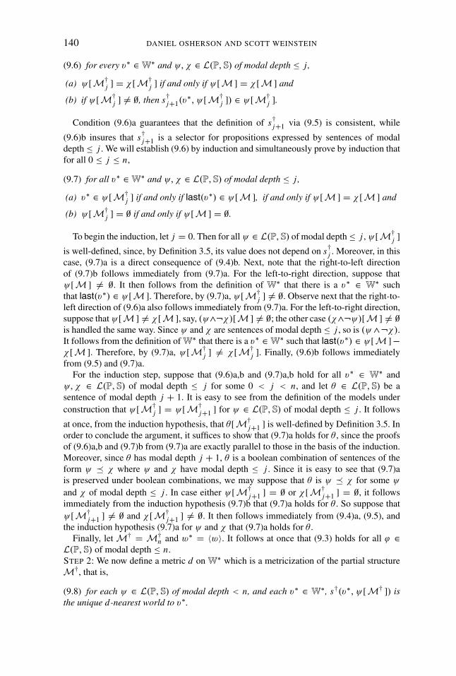
(9.6) for every v∗ ∈ W∗ and ψ,χ ∈ L(P, S) of modal depth ≤ j ,
(a) ψ[M†j ] = χ [M†
j ] if and only if ψ[M ] = χ [M ] and
(b) if ψ[M†j ] �= ∅, then s†
j+1(v∗, ψ[M†
j ]) ∈ ψ[M†j ].
Condition (9.6)a guarantees that the definition of s†j+1 via (9.5) is consistent, while
(9.6)b insures that s†j+1 is a selector for propositions expressed by sentences of modal
depth ≤ j . We will establish (9.6) by induction and simultaneously prove by induction thatfor all 0 ≤ j ≤ n,
(9.7) for all v∗ ∈ W∗ and ψ,χ ∈ L(P, S) of modal depth ≤ j ,
(a) v∗ ∈ ψ[M†j ] if and only if last(v∗) ∈ ψ[M ], if and only if ψ[M ] = χ [M ] and
(b) ψ[M†j ] = ∅ if and only if ψ[M ] = ∅.
To begin the induction, let j = 0. Then for all ψ ∈ L(P, S) of modal depth ≤ j , ψ[M†j ]
is well-defined, since, by Definition 3.5, its value does not depend on s†j . Moreover, in this
case, (9.7)a is a direct consequence of (9.4)b. Next, note that the right-to-left directionof (9.7)b follows immediately from (9.7)a. For the left-to-right direction, suppose thatψ[M ] �= ∅. It then follows from the definition of W∗ that there is a v∗ ∈ W
∗ suchthat last(v∗) ∈ ψ[M ]. Therefore, by (9.7)a, ψ[M†
j ] �= ∅. Observe next that the right-to-left direction of (9.6)a also follows immediately from (9.7)a. For the left-to-right direction,suppose that ψ[M ] �= χ [M ], say, (ψ∧¬χ)[M ] �= ∅; the other case (χ∧¬ψ)[M ] �= ∅is handled the same way. Since ψ and χ are sentences of modal depth ≤ j , so is (ψ ∧¬χ).It follows from the definition ofW∗ that there is a v∗ ∈ W∗ such that last(v∗) ∈ ψ[M ]−χ [M ]. Therefore, by (9.7)a, ψ[M†
j ] �= χ [M†j ]. Finally, (9.6)b follows immediately
from (9.5) and (9.7)a.For the induction step, suppose that (9.6)a,b and (9.7)a,b hold for all v∗ ∈ W
∗ andψ,χ ∈ L(P, S) of modal depth ≤ j for some 0 < j < n, and let θ ∈ L(P, S) be asentence of modal depth j + 1. It is easy to see from the definition of the models underconstruction that ψ[M†
j ] = ψ[M†j+1 ] for ψ ∈ L(P, S) of modal depth ≤ j . It follows
at once, from the induction hypothesis, that θ [M†j+1 ] is well-defined by Definition 3.5. In
order to conclude the argument, it suffices to show that (9.7)a holds for θ , since the proofsof (9.6)a,b and (9.7)b from (9.7)a are exactly parallel to those in the basis of the induction.Moreover, since θ has modal depth j + 1, θ is a boolean combination of sentences of theform ψ � χ where ψ and χ have modal depth ≤ j . Since it is easy to see that (9.7)ais preserved under boolean combinations, we may suppose that θ is ψ � χ for some ψ
and χ of modal depth ≤ j . In case either ψ[M†j+1 ] = ∅ or χ [M†
j+1 ] = ∅, it followsimmediately from the induction hypothesis (9.7)b that (9.7)a holds for θ . So suppose thatψ[M†
j+1 ] �= ∅ and χ[M†j+1 ] �= ∅. It then follows immediately from (9.4)a, (9.5), and
the induction hypothesis (9.7)a for ψ and χ that (9.7)a holds for θ .Finally, let M† = M†
n and w∗ = 〈w〉. It follows at once that (9.3) holds for all ϕ ∈L(P, S) of modal depth ≤ n.STEP 2: We now define a metric d on W∗ which is a metricization of the partial structureM†, that is,
(9.8) for each ψ ∈ L(P, S) of modal depth < n, and each v∗ ∈ W∗, s†(v∗, ψ[M† ]) isthe unique d-nearest world to v∗.
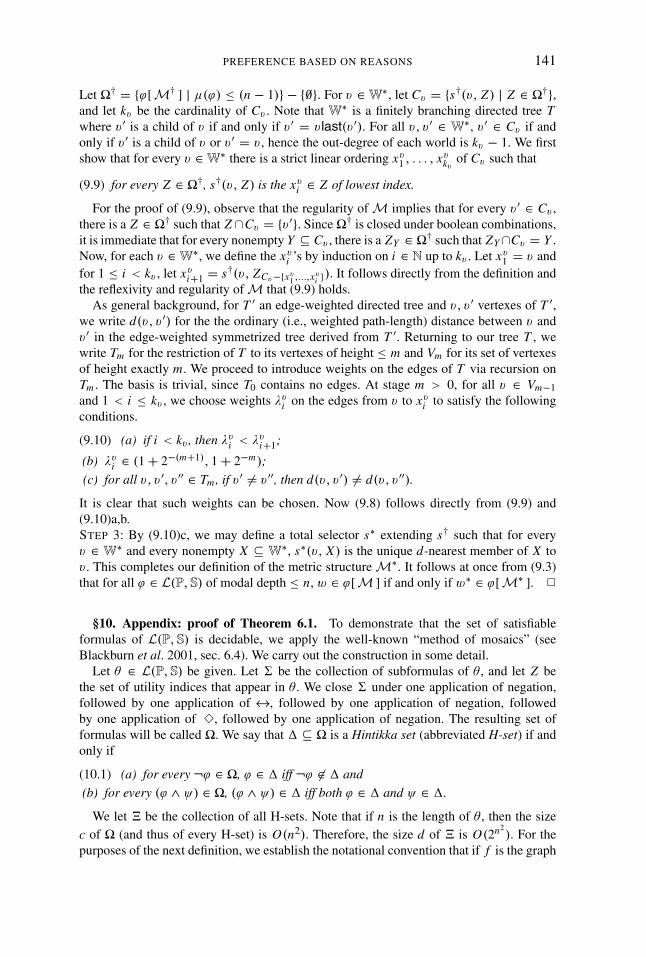
PREFERENCE BASED ON REASONS 141
Let † = {ϕ[M† ] | μ(ϕ) ≤ (n − 1)} − {∅}. For v ∈ W∗, let Cv = {s†(v, Z) | Z ∈ †},and let kv be the cardinality of Cv . Note that W∗ is a finitely branching directed tree Twhere v ′ is a child of v if and only if v ′ = v last(v ′). For all v, v ′ ∈ W∗, v ′ ∈ Cv if andonly if v ′ is a child of v or v ′ = v , hence the out-degree of each world is kv − 1. We firstshow that for every v ∈ W∗ there is a strict linear ordering xv
1 , . . . , xvkv
of Cv such that
(9.9) for every Z ∈ †, s†(v, Z) is the xvi ∈ Z of lowest index.
For the proof of (9.9), observe that the regularity ofM implies that for every v ′ ∈ Cv ,there is a Z ∈ † such that Z ∩Cv = {v ′}. Since † is closed under boolean combinations,it is immediate that for every nonempty Y ⊆ Cv , there is a ZY ∈ † such that ZY ∩Cv = Y .Now, for each v ∈ W∗, we define the xv
i ’s by induction on i ∈ N up to kv . Let xv1 = v and
for 1 ≤ i < kv , let xvi+1 = s†(v, ZCv−{xv
1 ,...,xvi }). It follows directly from the definition and
the reflexivity and regularity ofM that (9.9) holds.As general background, for T ′ an edge-weighted directed tree and v, v ′ vertexes of T ′,
we write d(v, v ′) for the the ordinary (i.e., weighted path-length) distance between v andv ′ in the edge-weighted symmetrized tree derived from T ′. Returning to our tree T , wewrite Tm for the restriction of T to its vertexes of height ≤ m and Vm for its set of vertexesof height exactly m. We proceed to introduce weights on the edges of T via recursion onTm . The basis is trivial, since T0 contains no edges. At stage m > 0, for all v ∈ Vm−1and 1 < i ≤ kv , we choose weights λv
i on the edges from v to xvi to satisfy the following
conditions.
(9.10) (a) if i < kv , then λvi < λv
i+1;
(b) λvi ∈ (1 + 2−(m+1), 1 + 2−m);
(c) for all v, v ′, v ′′ ∈ Tm, if v ′ �= v ′′, then d(v, v ′) �= d(v, v ′′).
It is clear that such weights can be chosen. Now (9.8) follows directly from (9.9) and(9.10)a,b.STEP 3: By (9.10)c, we may define a total selector s∗ extending s† such that for everyv ∈ W∗ and every nonempty X ⊆ W
∗, s∗(v, X) is the unique d-nearest member of X tov . This completes our definition of the metric structureM∗. It follows at once from (9.3)that for all ϕ ∈ L(P, S) of modal depth ≤ n, w ∈ ϕ[M ] if and only if w∗ ∈ ϕ[M∗ ]. 2
§10. Appendix: proof of Theorem 6.1. To demonstrate that the set of satisfiableformulas of L(P, S) is decidable, we apply the well-known “method of mosaics” (seeBlackburn et al. 2001, sec. 6.4). We carry out the construction in some detail.
Let θ ∈ L(P, S) be given. Let be the collection of subformulas of θ , and let Z bethe set of utility indices that appear in θ . We close under one application of negation,followed by one application of ↔, followed by one application of negation, followedby one application of 3, followed by one application of negation. The resulting set offormulas will be called . We say that ⊆ is a Hintikka set (abbreviated H-set) if andonly if
(10.1) (a) for every ¬ϕ ∈ , ϕ ∈ iff ¬ϕ �∈ and
(b) for every (ϕ ∧ ψ) ∈ , (ϕ ∧ ψ) ∈ iff both ϕ ∈ and ψ ∈ .
We let � be the collection of all H-sets. Note that if n is the length of θ , then the sizec of (and thus of every H-set) is O(n2). Therefore, the size d of � is O(2n2
). For thepurposes of the next definition, we establish the notational convention that if f is the graph

142 DANIEL OSHERSON AND SCOTT WEINSTEIN
of a partial function, we write f (a) for the b such that 〈a, b〉 ∈ f , when a is in the domainof f . A brick is a triple 〈 ,σ, {υX | X ∈ Z}〉 where
(10.2) (a) is an H-set;
(b) σ is the graph of a partial function from into � such that ϕ ∈ σ(ϕ) for every ϕ ∈ on which σ is defined;
(c) for each X ∈ Z, υX is a function from σ to {i | 1 ≤ i ≤ card(σ )};(d) if ♦ϕ ∈ , then for some ′ ∈ range(σ ), ϕ ∈ ′;(e) if ♦ϕ �∈ , then for all ′ ∈ range(σ ) ∪ { }, ϕ �∈ ′;(f) �(ϕ ↔ ψ) ∈ if and only if σ(ϕ) = σ(ψ);
(g) (ϕ �X ψ) ∈ iff υX (〈ϕ, σ(ϕ)〉) ≤ υX (〈ψ, σ(ψ)〉).Let z be the size of Z . Note that the number b of bricks is O(dc+1 · ccz).If β is a brick, we write β1, β2, and β3 for the first, second, and third coordinates of β.
A set B of bricks is a mosaic if and only if
(10.3) (a) for all β, β ′ ∈ B, {ϕ | ♦ϕ ∈ β1} = {ϕ | ♦ϕ ∈ β ′1} and
(b) for all β ∈ B and for all ∈ range(β2) there is a β ′ ∈ B such that β ′1 = .
A set B of bricks is a mosaic for θ ∈ L(P, S) if and only if B is a mosaic and forsome β ∈ B, θ ∈ β1. Note that the number of mosaics is O(2b) and that it is decidable intime polynomial in the size of a set B of bricks whether B is a mosaic. It follows that thedecision problem “Does there exist a mosaic for θ” is in NTIME(b). Theorem 6.1 is thus acorollary to the following.
PROPOSITION 10.4. For every θ ∈ L(P, S), θ is satisfiable if and only if there is a mosaicfor θ .
To prove the left to right direction of Proposition 10.4, let satisfiable θ ∈ L(P, S) begiven. For notational convenience we assume that Z = {X}. The generalization to multipleutility indices is routine. Let model M = (W, s, u, t) satisfy θ and suppose that w0 ∈θ [M ]. For each w ∈ W, let w = {ϕ ∈ | w ∈ ϕ[M ]}. Note that for every w ∈ W, w is an H-set. Now for each w ∈ W, we construct a brick βw = 〈 w, σw, υw〉, where foreach ϕ ∈ ,
σw(ϕ) = s(w,ϕ[M ])
and for all ϕ,ψ ∈ w
υw(〈ϕ, σw(ϕ)〉) ≤ υw(〈ψ, σw(ψ)〉) iff u(s(w, ϕ[M ])) ≤ u(s(w,ψ[M ])).
Let B = {βw | w ∈ W}. It is easy to verify that B is a mosaic for θ .For the right to left direction of Proposition 10.4, suppose that B is a mosaic for θ . We
show how to use the bricks of B to construct a tree-like infinite modelM = (W, s, u, t),the root world w0 of which satisfies θ . The tree underlying the model is both node-labeledand edge-labeled. We call the node labels “brick-labels” and we call the edge labels“selector-labels.” The construction of the tree proceeds by induction; at stage i , we con-struct the worlds of depth i .
At stage 0 we introduce a world w0 and label w0 with some brick β ∈ B such thatθ ∈ β1 (such a brick-label exists, since B is a mosaic for θ ).
Let Wn be the set of worlds constructed at stage n. At stage n +1 we proceed as follows.For each w ∈ Wn we construct the children of w as follows. Let βw = 〈 w, σw, υw〉 bethe brick-label of w. For each ∈ range(σw) we introduce a child w′ of w; we label the
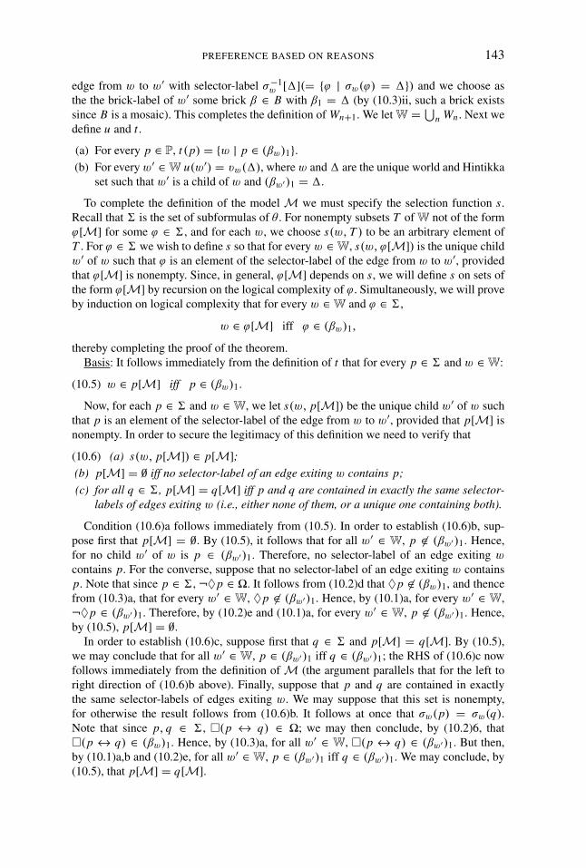
PREFERENCE BASED ON REASONS 143
edge from w to w′ with selector-label σ−1w [ ](= {ϕ | σw(ϕ) = }) and we choose as
the the brick-label of w′ some brick β ∈ B with β1 = (by (10.3)ii, such a brick existssince B is a mosaic). This completes the definition of Wn+1. We letW = ⋃
n Wn . Next wedefine u and t .
(a) For every p ∈ P, t (p) = {w | p ∈ (βw)1}.(b) For every w′ ∈ W u(w′) = υw( ), where w and are the unique world and Hintikka
set such that w′ is a child of w and (βw′)1 = .
To complete the definition of the model M we must specify the selection function s.Recall that is the set of subformulas of θ . For nonempty subsets T ofW not of the formϕ[M] for some ϕ ∈ , and for each w, we choose s(w, T ) to be an arbitrary element ofT . For ϕ ∈ we wish to define s so that for every w ∈ W, s(w, ϕ[M]) is the unique childw′ of w such that ϕ is an element of the selector-label of the edge from w to w′, providedthat ϕ[M] is nonempty. Since, in general, ϕ[M] depends on s, we will define s on sets ofthe form ϕ[M] by recursion on the logical complexity of ϕ. Simultaneously, we will proveby induction on logical complexity that for every w ∈ W and ϕ ∈ ,
w ∈ ϕ[M] iff ϕ ∈ (βw)1,
thereby completing the proof of the theorem.Basis: It follows immediately from the definition of t that for every p ∈ and w ∈ W:
(10.5) w ∈ p[M] iff p ∈ (βw)1.
Now, for each p ∈ and w ∈ W, we let s(w, p[M]) be the unique child w′ of w suchthat p is an element of the selector-label of the edge from w to w′, provided that p[M] isnonempty. In order to secure the legitimacy of this definition we need to verify that
(10.6) (a) s(w, p[M]) ∈ p[M];
(b) p[M] = ∅ iff no selector-label of an edge exiting w contains p;
(c) for all q ∈ , p[M] = q[M] iff p and q are contained in exactly the same selector-labels of edges exiting w (i.e., either none of them, or a unique one containing both).
Condition (10.6)a follows immediately from (10.5). In order to establish (10.6)b, sup-pose first that p[M] = ∅. By (10.5), it follows that for all w′ ∈ W, p �∈ (βw′)1. Hence,for no child w′ of w is p ∈ (βw′)1. Therefore, no selector-label of an edge exiting wcontains p. For the converse, suppose that no selector-label of an edge exiting w containsp. Note that since p ∈ , ¬♦p ∈ . It follows from (10.2)d that ♦p �∈ (βw)1, and thencefrom (10.3)a, that for every w′ ∈ W, ♦p �∈ (βw′)1. Hence, by (10.1)a, for every w′ ∈ W,¬♦p ∈ (βw′)1. Therefore, by (10.2)e and (10.1)a, for every w′ ∈ W, p �∈ (βw′)1. Hence,by (10.5), p[M] = ∅.
In order to establish (10.6)c, suppose first that q ∈ and p[M] = q[M]. By (10.5),we may conclude that for all w′ ∈ W, p ∈ (βw′)1 iff q ∈ (βw′)1; the RHS of (10.6)c nowfollows immediately from the definition ofM (the argument parallels that for the left toright direction of (10.6)b above). Finally, suppose that p and q are contained in exactlythe same selector-labels of edges exiting w. We may suppose that this set is nonempty,for otherwise the result follows from (10.6)b. It follows at once that σw(p) = σw(q).Note that since p, q ∈ , �(p ↔ q) ∈ ; we may then conclude, by (10.2)6, that�(p ↔ q) ∈ (βw)1. Hence, by (10.3)a, for all w′ ∈ W, �(p ↔ q) ∈ (βw′)1. But then,by (10.1)a,b and (10.2)e, for all w′ ∈ W, p ∈ (βw′)1 iff q ∈ (βw′)1. We may conclude, by(10.5), that p[M] = q[M].

144 DANIEL OSHERSON AND SCOTT WEINSTEIN
Induction Hypothesis: Suppose that for all w ∈ W,
(10.7) (a) w ∈ ϕ[M] iff ϕ ∈ (βw)1;
(b) w ∈ ψ[M] iff ψ ∈ (βw)1;
(c) s(w, ϕ[M]) and s(w,ψ[M]) are determined.
Induction Step: It follows immediately from (10.1)a,b and (10.7)a,b that for all w ∈ W,
w ∈ (ϕ ∧ ψ)[M] iff (ϕ ∧ ψ) ∈ (βw)1
and
w ∈ (¬ϕ)[M] iff (¬ϕ) ∈ (βw)1.
It remains to show that
w ∈ (ϕ � ψ)[M] iff (ϕ � ψ) ∈ (βw)1.
Suppose first that w ∈ (ϕ � ψ)[M]. Then, s(w, ϕ[M]) and s(w,ψ[M]) are bothdefined and υw(s(w, ϕ[M])) = u(s(w, ϕ[M])) ≤ u(s(w,ψ[M])) = υw(s(w,ψ[M])).It follows at once, by (10.2)g and (10.7)a,b, that (ϕ � ψ) ∈ (βw)1. Suppose, on the otherhand, that w �∈ (ϕ � ψ)[M]. Then either at least one of ϕ[M] or ψ[M] is empty, orυw(s(w,ψ[M])) = u(s(w,ψ[M])) < u(s(w, ϕ[M])) = υw(s(w, ϕ[M])). In eithercase, it follows from (10.7)a,b, (10.1)a, and (10.2)g, that (ϕ � ψ) �∈ (βw)1.
The extension of the definition of s to (ϕ ∧ ψ)[M], (¬ϕ)[M], and (ϕ � ψ)[M] isjustified exactly as in the basis of the induction. 2
The above argument may be adapted to establish Corollaries 6.2 and 6.3.
Proof of Corollary 6.2. We modify the construction of (W, s, u, t) in the argument forthe right to left direction of Proposition 10.4 to build a finite model satisfying θ from amosaic B for θ . Let W = ⋃
n Wn be the set of worlds constructed in the proof above, andlet n be the first stage such that for every w ∈ W there is an m < n and a w′ ∈ Wm suchthat βw = βw′ . We now close the construction of (W, s, u, t) at stage n + 1 by choosingthe children of each w ∈ Wn to be suitable worlds in
⋃m≤n Wm that satisfy the conditions
in the construction of (W, s, u, t). �
Proof of Corollary 6.3. We modify the definition of brick as follows. A reflexive brickB = 〈 ,σ, υ〉 is a brick that satisfies the following additional condition:
(10.8) for all ϕ ∈ , s(ϕ) = .
A reflexive mosaic is a mosaic composed of reflexive bricks; a reflexive mosaic for θ isdefined similarly. Corollary 6.3 follows from the next proposition.
PROPOSITION 10.9. For every θ ∈ L(P, S), θ is satisfiable in a reflexive model if and onlyif there is a reflexive mosaic for θ .
The proof of Proposition 10.9 is a straightforward adaptation of the proof of Proposition10.4. The only subtlety is that in the definition of the tree-like model (W, s, u, t) we canno longer define u in advance, but must define it by recursion following the recursiveconstruction of the tree. We extend the definition of u to the children of a world w bychoosing rational values for the children in such a way as to establish an isomorphism withthe order induced by υw, remembering that w will be chosen as a child of w in the obviousway, so that u must retain the value for w that was determined at stage n. �
PREFERENCE BASED ON REASONS 145
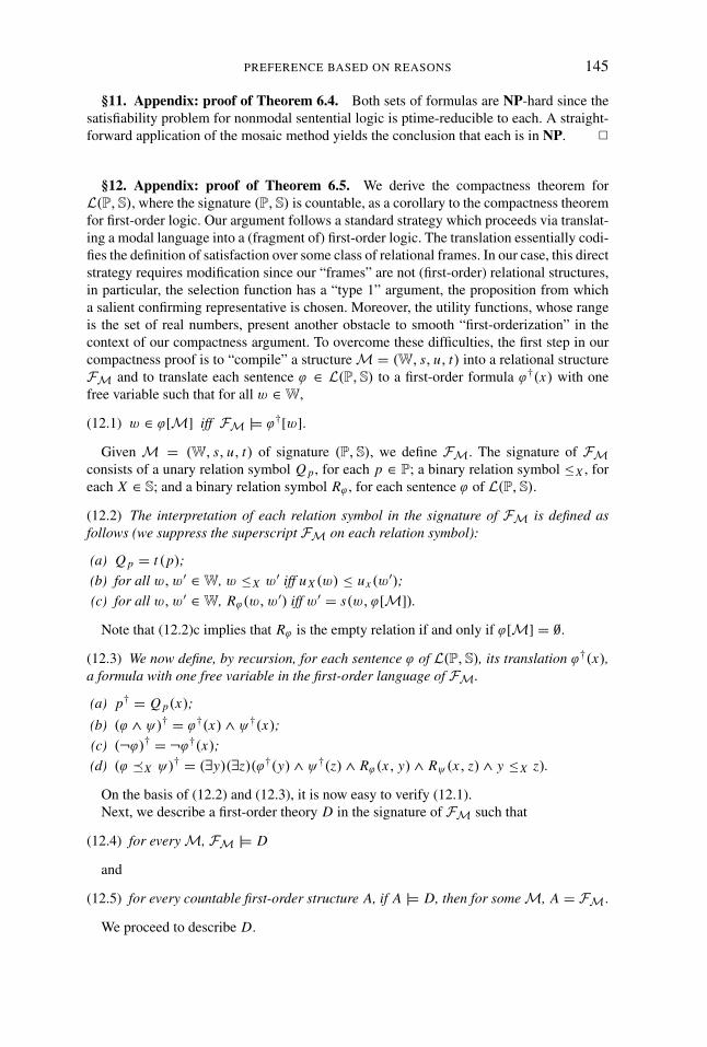
§11. Appendix: proof of Theorem 6.4. Both sets of formulas are NP-hard since thesatisfiability problem for nonmodal sentential logic is ptime-reducible to each. A straight-forward application of the mosaic method yields the conclusion that each is in NP. 2
§12. Appendix: proof of Theorem 6.5. We derive the compactness theorem forL(P, S), where the signature (P, S) is countable, as a corollary to the compactness theoremfor first-order logic. Our argument follows a standard strategy which proceeds via translat-ing a modal language into a (fragment of) first-order logic. The translation essentially codi-fies the definition of satisfaction over some class of relational frames. In our case, this directstrategy requires modification since our “frames” are not (first-order) relational structures,in particular, the selection function has a “type 1” argument, the proposition from whicha salient confirming representative is chosen. Moreover, the utility functions, whose rangeis the set of real numbers, present another obstacle to smooth “first-orderization” in thecontext of our compactness argument. To overcome these difficulties, the first step in ourcompactness proof is to “compile” a structureM = (W, s, u, t) into a relational structureFM and to translate each sentence ϕ ∈ L(P, S) to a first-order formula ϕ†(x) with onefree variable such that for all w ∈ W,
(12.1) w ∈ ϕ[M] iff FM |� ϕ†[w].
Given M = (W, s, u, t) of signature (P, S), we define FM. The signature of FMconsists of a unary relation symbol Q p, for each p ∈ P; a binary relation symbol ≤X , foreach X ∈ S; and a binary relation symbol Rϕ , for each sentence ϕ of L(P, S).
(12.2) The interpretation of each relation symbol in the signature of FM is defined asfollows (we suppress the superscript FM on each relation symbol):
(a) Q p = t (p);
(b) for all w,w′ ∈ W, w ≤X w′ iff uX (w) ≤ ux (w′);
(c) for all w,w′ ∈ W, Rϕ(w,w′) iff w′ = s(w, ϕ[M]).
Note that (12.2)c implies that Rϕ is the empty relation if and only if ϕ[M] = ∅.
(12.3) We now define, by recursion, for each sentence ϕ of L(P, S), its translation ϕ†(x),a formula with one free variable in the first-order language of FM.
(a) p† = Q p(x);
(b) (ϕ ∧ ψ)† = ϕ†(x) ∧ ψ†(x);
(c) (¬ϕ)† = ¬ϕ†(x);
(d) (ϕ �X ψ)† = (∃y)(∃z)(ϕ†(y) ∧ ψ†(z) ∧ Rϕ(x, y) ∧ Rψ(x, z) ∧ y ≤X z).
On the basis of (12.2) and (12.3), it is now easy to verify (12.1).Next, we describe a first-order theory D in the signature of FM such that
(12.4) for everyM, FM |� D
and
(12.5) for every countable first-order structure A, if A |� D, then for someM, A = FM.
We proceed to describe D.
146 DANIEL OSHERSON AND SCOTT WEINSTEIN
(12.6) D consists of the following first-order sentences.
(a) (∀x)(∀y)(∀z)(x ≤X y → (y ≤X z → x ≤X z)), for each X ∈ S;
(b) (∀y)(y ≤X y), for each X ∈ S;
(c) (∀y)(∀z)(y ≤X z ∨ z ≤X y), for each X ∈ S;
(d) (∀x)(∀y)(Rϕ(x, y) → ϕ†(y)), for each ϕ ∈ L(P, S);
(e) (∃x)ϕ†(x) → (∀x)(∃y)(∀z)(Rϕ(x, z) ↔ y = z), for each ϕ ∈ L(P, S);
(f) (∀x)(ϕ(x) ↔ ψ(x)) → (∀x)(∀y)(Rϕ(x, y) ↔ Rψ(x, y)), for each ϕ,ψ ∈ L(P, S).
It is easy to verify (12.4) by direct inspection of the clauses of (12.6). In order to verify(12.5), we argue as follows. Let A be a countable relational structure satisfying D. Wedefine a structureM = (W, s, u, t). First, letW = |A| and let t (p) = Q A
p , for each p ∈ P.
Next, by (12.6)a–c, for each X ∈ S, ≤AX is a countable linear preorder. It follows from the
universality of the rational numbers among countable linear orders that a utility functionu X may be chosen so that for all w,w′ ∈ W, w ≤X w′ if and only if u X (w) ≤ u X (w′). Foreach ϕ ∈ L(P, S) and w,w′ ∈ W, let s(w, ϕ[M]) = w′ if and only if Rϕ(w,w′). Finally,let s(w, P) be an arbitrarily chosen element of P for any proposition P ⊆ W which is notexpressed by a sentence. It is easy to see that the structureM satisfies (12.5).
We now derive Theorem 6.5 from the compactness theorem for first-order logic. Let Tbe a set of sentences of L(P, S) and suppose that every finite subset T ′ ⊆ T is satisfiable. Itfollows at once from (12.1) and (12.4) that for every finite T ′ ⊆ T , {ϕ†(c) | ϕ ∈ T ′}∪ D issatisfiable (here c is a constant symbol). Therefore, by the Compactness and Lowenheim–Skolem Theorems for first-order logic, there is a countable structure A such that A |�{ϕ†(c) | ϕ ∈ T } ∪ D. Hence, by (12.1) and (12.5), T is satisfiable. 2
BIBLIOGRAPHY
Andreka, H., Ryan, M., & Schobbens, P.-Y. (2002). Operators and laws for combiningpreferential relations. Journal of Logic and Computation, 12, 12–53.
Blackburn, P., de Rijke, M., & Venema, Y. (2001). Modal Logic. New York, NY:Cambridge University Press.
Dietrich, F., & List, C. (2009). A Reason-Based Theory of Rational Choice. TechnicalReport, London School of Economics.
Gardenfors, P. (1988). Knowledge in Flux: Modeling the Dynamics of Epistemic States.Cambridge, MA: MIT Press.
Haidt, J. (2001). The emotional dog and its rational tail: A social intuitionist approach tomoral judgment. Psychological Review, 108, 814–834.
Johnson, P. E. (1988). Social Choice: Theory and Research. New York, NY: SagePublications.
Keeney, R. L., & Raiffa, H. (1993). Decisions with Multiple Objectives: Preferences andValue Trade-Offs. Cambridge, UK: Cambridge University Press.
Lang, J., van der Torre, L., & Weydert, E. (2003). Hidden uncertainty in the logicalrepresentation of desires. In Proceedings of Eighteenth International Joint Conferenceon Artificial Intelligence (IJCAI03). San Francisco, CA: Morgan Kaufmann.
Levi, I. (1986). Hard Choices: Decision Making under Unresolved Conflict. Cambridge,UK: Cambridge University Press.
Lewis, D. (1973). Counterfactuals. Cambridge, MA: Harvard University Press.Liu, F. (2008). Changing for the better: Preference dynamics and agent diversity. PhD
Thesis, ILLC, University of Amsterdam.
PREFERENCE BASED ON REASONS 147
Messick. D. M. (1985). Social interdependence and decision making. In Wright, G., editor.Behavioral Decision Making. New York, NY: Plenum, pp. 87–109.
Osherson, D., & Weinstein, S. (To appear). Modal logic for preference based on reasons.In Tannen, V., editor. Lecture Notes in Computer Science. New York, NY: Springer.
Osherson, D., & Weinstein, S. (Forthcoming). Two approaches to the logic of preference.Payne, J. W., & Puto, C. (1982). Adding asymmetrically dominated alternatives: Violations
of regularity and the similarity hypothesis. The Journal of Consumer Research, 9, 90–95.Pettit, P. (2002). Rules, Reasons, and Norms. Oxford, UK: Oxford University Press.Savage, L. J. (1954). The Foundations of Statistics. New York, NY: Wiley.Sen, A. (1971). Choice functions and revealed preference. Review of Economic Studies,
38, 307–317.Stalnaker, R. (1968). A theory of conditionals. In Rescher, N., editor. Studies in logical
theory. Oxford, UK: Blackwell.Tentori, K., Osherson, D., Hasher, L., & May, C. (2001). Wisdom and aging: Irrational
preferences in college students but not older adults. Cognition, 81, B87–B96.van Benthem, J., Girard, P. K., & Roy, O. (2009). Everything else being equal: A modal
logic for Ceteris Paribus preferences. Journal of Philosophical Logic, 38, 83–125.van Benthem, J., & Liu, F. (2007). Dynamic logic of preference upgrade. Journal of
Applied Non-Classical Logic, 17, 157–182.von Wright, G. H. (1963). The Logic of Preference. Edinburgh, UK: Edinburgh University
Press.
DEPARTMENT OF PSYCHOLOGYPRINCETON UNIVERSITY
PRINCETON NJ 08540 USAE-mail: [email protected]
DEPARTMENT OF PHILOSOPHYUNIVERSITY OF PENNSYLVANIA
PHILADELPHIA PA 19104 USAE-mail: [email protected]