Embed Size (px)
Citation preview
IEEE TRANSACTIONS ON GEOSCIENCE AND REMOTE SENSING 6257
Subspace-Based Technique for SpeckleNoise Reduction in SAR Images
Norashikin Yahya, Member, IEEE, Nidal S. Kamel, Senior Member, IEEE, andAamir Saeed Malik, Senior Member, IEEE
Abstract—Image-subspace-based approach for speckle noise re-moval from synthetic aperture radar (SAR) images is proposed.The underlying principle is to apply homomorphic framework inorder to convert multiplicative speckle noise into additive and thento decompose the vector space of the noisy image into signal andnoise subspaces. Enhancement is performed by nulling the noisesubspace and estimating the clean image from the remaining sig-nal subspace. Linear estimator minimizing image distortion whilemaintaining the residual noise energy below some given thresholdis used to estimate the clean image. Experiments are carried outusing synthetically generated data set with controlled statistics andreal SAR image of Selangor area in Malaysia. The performance ofthe proposed technique is compared with Lee and homomorphicwavelet in terms of noise variance reduction and preservation ofradiometric edges. The results indicate moderate noise reductionby the proposed filter in comparison to Lee but with a significantlyless blurry effect and a comparable performance in terms ofnoise reduction to wavelet but with less artifacts. The results alsoshow better preservation of edges, texture, and point targets bythe proposed filter than both Lee and wavelet and less requiredcomputational time.
Index Terms—Image denoising, principal component analy-sis (PCA), spatial filters, stochastic processes, synthetic apertureradar (SAR).
I. INTRODUCTION
THE synthetic aperture radar (SAR) imaging technique ispopular for remote sensing and monitoring applications
because of its usability under various weather conditions andits ability to provide high-resolution imagery. A SAR imageis generated by sending electromagnetic waves from a movingplatform, spaceborne or airborne, toward the target surface andby coherently processing the returned backscattered signalsfrom multiple distributed targets [1]. However, the coherentprocessing causes speckle effect [2] and gives SAR images itsnoisy appearance. Speckle presence appears as granular noisewhich reduces the image resolution [3] and may hamper theoperation of image interpretation and analysis. Hence, noisefiltering has become an essential part of SAR imagery systems.The objective of using a speckle reduction filter is to smoothhomogeneous regions while preserving the useful textural in-
Manuscript received March 17, 2013; revised September 5, 2013 andNovember 27, 2013; accepted December 9, 2013.
The authors are with the Department of Electrical and Electronic Engi-neering, Universiti Teknologi PETRONAS, 31750 Tronoh, Malaysia (e-mail:[email protected]).
Color versions of one or more of the figures in this paper are available onlineat http://ieeexplore.ieee.org.
Digital Object Identifier 10.1109/TGRS.2013.2295824
formation and structural features, such as edges. In subsequentparagraphs, we discuss the different types of adaptive filters thatare used to reduce speckle noise in SAR images.
The commonly used adaptive spatial-domain filters forspeckle reduction are Lee filter [4], Frost filter [5], Kuan filter[6], and enhanced Lee and modified Frost filters [7]. Theassumptions made in implementing these filters are as follows:1) The SAR speckle is modeled as a multiplicative noise; 2) thenoise and signal are statistically independent; and 3) the samplemean and variance of a pixel are equal to its local mean andlocal variance computed within a window centered on the pixelof interest [4], [8]. The performance of these filters is highlydependent on the choice of size and orientation of the movingwindow.
The Lee and Kuan filters have similar formation but differin signal model assumptions and derivation. They originatefrom simplified theoretical studies and are based on parametersrelated to local image coefficients of variation which measuresthe scene heterogeneity [9]. Both Lee and Kuan filters removespeckle noise by computing a linear combination of the centerpixel intensity in a filter window with an average intensityof the window. Thus, the filters achieve a balance betweenaveraging in homogeneous regions and a strict all-pass (iden-tity) filter in edge contained regions. On the other hand, theFrost filter attempts to strike a balance between averaging andidentity filter by forming an exponential-shaped filter kernelthat can adaptively vary from an average filter to an identityfilter. Similar to Lee and Kuan filters, the filter response varieslocally with the coefficients of variation. This means that, atlow coefficient variation, the filter is more average-like and, athigh coefficient variation, the filter attempts to preserve sharpfeatures by retaining its original pixel value. The enhanced Leeand Frost filter proposed by Lopes et al. [7] uses three variationsof coefficient values, namely, low, intermediate, and high, todivide an image into homogeneous regions, heterogeneousregions, and isolated point target regions, respectively. The filteroutputs a local mean at homogeneous regions and retains theoriginal pixel at points of high activity. Generally speaking, theadaptive spatial-domain filters have the following deficiencies:1) fail to maintain the mean value, particularly if the number oflook of the original SAR data is small; 2) the highly reflectivepoint targets are blurred; and 3) dark spotty pixels are notfiltered [10].
In addition to the averaging and adaptive filters, there isspeckle noise removal using wavelet transform [11]–[13]. Asan outcome of wavelet theory, denoising in the discrete wavelettransform (DWT) domain may be stated as a thresholding
0196-2892 © 2014 IEEE. Personal use is permitted, but republication/redistribution requires IEEE permission.See http://www.ieee.org/publications_standards/publications/rights/index.html for more information.
6258 IEEE TRANSACTIONS ON GEOSCIENCE AND REMOTE SENSING
of DWT coefficients of the noisy image. For the case ofspeckle noise, homomorphic filtering, in which the DWT of thelog-transformed noisy image is either adaptively thresholded[14] or empirically shrunk in an adaptive fashion [15], hasbeen utilized. The major drawbacks of such approach are thebackscatter mean preservation in homogeneous areas, sharp-ness preservation, and ringing impairments [15], [16]. Further-more, signal variations are damped by the logarithm, resultingin an unlikely “flatness” after filtering. To overcome thesedeficiencies, Argenti et al. in [17] proposed a minimum-mean-square error filtering performed in the undecimated wavelet do-main by means of an adaptive rescaling of the detail coefficientsand the local space-varying signal, where the noise statisticsare estimated in the wavelet domain. In [18], using statisticalmodeling of wavelet coefficients, Ranjani et al. proposed aspeckle suppression technique using dual-tree wavelet trans-form by putting into consideration the significant dependencesof the wavelet coefficients across different scales. The interscaledependence of the wavelet coefficients in each subband is mod-eled using bivariate Cauchy probability density function (pdf).
In this paper, a subspace-based technique to reduce thespeckle noise in SAR images is proposed. Fundamentally, theproposed technique is an extension of the original work ofEphraim and Van Trees [19] in speech enhancement toward 2-Dsignals. The underlying principle is to decompose the vectorspace of the noisy image into a signal-plus-noise subspace andthe noise subspace. The noise removal is achieved by nulling thenoise subspace and controlling the noise distribution in the signalsubspace. For white noise, the subspace decomposition cantheoretically be performed by applying the Karhunen-Loevetransform (KLT) to the noisy image. Linear estimator of the cleanimage is performed by minimizing image distortion while main-taining the residual noise energy below some given threshold.For colored noise, a prewhitening approach prior to KLT trans-form, or a generalized subspace for simultaneous diagonaliza-tion of the clean and noise covariance matrices, can be used.
The fundamental signal and noise model for subspace meth-ods is additive noise uncorrelated with the signal. However,in SAR images, the noise is multiplicative in nature, so ahomomorphic framework takes advantage of logarithmic trans-formation in order to convert multiplicative noise into additivenoise. However, this nonlinear operation totally changes thestatistics of SAR images and induces bias in their mean values.For the purpose of radiometric preservation, the biased meanneeds to be corrected, along with antilog operation.
This paper is organized as follows. Section II describes thepdf of speckle noise in SAR images. Section III, covers theprinciple of subspace and how it can be extended to specklenoise removal. In specific, the first part of Section III coversthe proposed subspace technique and its implementation inspeckle noise filtering, the conceptual relationship betweeneigendecomposition and oriented energy, and the derivation ofthe optimal estimator using the principal subspace. The secondpart of Section III covers the implementation issues, namely, theestimation of noise variance, the method to determine the signalsubspace dimension, and the optimum value of the Lagrangemultiplier. Section IV is divided into two main sections. Thefirst part of Section IV evaluates the performance of SDC
for varying image size and its ability to represent images.The second part of Section IV evaluates the performance ofthe proposed technique using simulated images and real SARimages in comparison to Lee filter and a wavelet filter [20], [21]in homomorphic framework. Finally, Section V concludes thispaper.
For clarity, an attempt has been made to adhere to a stan-dard notational convention. Lowercase boldface characters willgenerally refer to vectors. Uppercase characters will generallyrefer to matrices. Vector or matrix transposition will be denotedusing (.)T , while transformations at the left and right sides aredenoted as (.)L and (.)R, respectively. Rm×m denotes the realvector space of m×m dimensions.
II. STATISTICAL MODELING OF SPECKLE
NOISE IN SAR IMAGES
With homogeneous targets and weakly textured areas inSAR images, the speckle noise is fully developed, and themultiplicative model is used to describe it. Since most availableimage denoising techniques were developed for additive whiteGaussian noise (AWGN), it is necessary in case of a fullydeveloped speckle noise to apply a logarithmic transform to themultiplicative model in order to convert it into additive. Theprocess involves applying logarithmic transform prior to the de-noising technique and then exponentially transforming the out-put to obtain the despeckled image. As a nonlinear operation,the logarithmic transform totally changes the statistics of SARimages, so the original speckle statistics cannot directly be usedwith the log-transformed images. In this section, the pdf, mean,and standard deviation values of the log-transformed specklenoise are briefly discussed. The purpose is to correct the biasedmean for radiometric preservation.
Speckle in SAR images is caused by constructive and de-structive interferences of coherent waves reflected by manyelementary scatterers contained within the image resolutioncell. Under the assumption that in each resolution cell: 1) noscatterers in domination over the others combined; 2) the num-ber of scatterers is large and they are statistically identical andindependent; and 3) the maximum range extent of the target ismany wavelength across, it then follows that the vector sum ofthe backscattered electric field is equivalent to a 2-D randomwalk process with independently and identically distributed(i.i.d.) Gaussian real and imaginary components [22], [23].
SAR images are usually available in two formats: intensityand amplitude. For homogeneous areas, the pdf of the magni-tude of the fully developed speckle is known to have Rayleighdistribution, and the phase is uniformly distributed. On the otherhand, the pdf of speckle intensity is described by a negativeexponential distribution [22], [23].
In SAR images, pixels are averaged in order to reduce thegrainy appearance caused by the speckle noise. In this case, thestatistical distribution of the resultant speckle noise is given bygamma distribution for intensity and by the multiconvolutionof the Rayleigh pdf in the case of amplitude format [16]. In thesubsequent paragraphs, the pdfs, mean values, and variances forthe logarithmically transformed speckle noise in intensity andamplitude format are discussed.
YAHYA et al.: SUBSPACE-BASED TECHNIQUE FOR SPECKLE NOISE REDUCTION IN SAR IMAGES 6259
A. Intensity Format
If we use G to denote the SAR image intensity for a givenpixel whose backscattering coefficients are W and assume thatthe SAR image is an average of L looks, then G is related to Wby the multiplicative model [23]
G = WN (1)
where N ∈ Rm×n is the random variable speckle noise matrix
following a gamma distribution with unit mean and variance,1/L. The noise pdf is given by [23]
PN (N) =LLNL−1e−LN
Γ(L), N ≥ 0 (2)
where Γ(.) denotes the gamma function. Applying the logarith-mic function to both sides of (1), we get
log(G) = log(W ) + log(N). (3)
Expression (3) can be rewritten as
Yl = Xl +Nl (4)
where Yl, Xl, and Nl are the logarithms of G, W , and N ,respectively. The mean and variance of the logarithmicallytransformed gamma distribution are given, respectively, by [16]
N̄l =ψ(0, L)− ln(L) (5)
v2Nl=ψ(1, L) (6)
where ψ(i, L) is the polygamma function of L-looks given by
ψ(i, z) =
(d
dz
)i
ψ(z) =
(d
dz
)i+1
ln Γ(z). (7)
When L is an integer, (6) can be further simplified to
N̄l =
L−1∑k=1
1
k+ ψ(1)− ln(L), ψ(1) = −C (8)
where C is the Euler’s constant (C = 0.577215) [16]. More-over, the variance can be computed from [24], [25]
v2Nl= ψ(1, 1)−
L−1∑k=1
1
k2, ψ(1, 1) =
π2
6. (9)
Table I shows the mean and standard deviation of Rayleigh-fading object as a function of the number of look (L) [24]. Thecalculated values in Table I can be used to adjust the bias inthe mean value due to homomorphic operations. It should bestressed that the bias does not depends on the mean value ofthe SAR intensity, which means that the bias can be correctedsystematically, provided that the number of looks is rightlyestimated.
TABLE IMEAN AND STANDARD DEVIATION OF SPECKLE NOISE
IN LINEAR AND LOGARITHMIC SCALES [24]
B. Amplitude Format
If (1) is in amplitude format and L = 1, then the pdf of Nobeys the Rayleigh pdf [23], and the mean and variance of itslogarithmic transform are given by
N̄l =1
2ln
(4
π
)+
1
2ψ(1), v2Nl
=1
4ψ(1, 1). (10)
For L > 1 amplitude image, different techniques are used toobtain a closed analytical form for the pdf. Among thesetechniques, there are histogram estimation technique and ap-proximation method using Edgeworth expansion [16].
Because of the simplicity in biased mean adjustment ofintensity format in comparison to the amplitude format, weconsider it for the analytical part of this paper.
III. SUBSPACE-BASED SPATIAL DOMAIN
CONSTRAINT APPROACH (SDC)
In this section, we derive the linear optimal estimator whichminimizes the image distortion while constraining the energy ofresidual noise. The noise is assumed to be AWGN, uncorrectedwith the signal. However, with SAR imagery, a colored noisedue to interpixel correlation in range because of oversamplingis usually developed. Thus, a whitening scheme should be usedprior to the implementation of the proposed subspace techniquein SAR applications. Different whitening schemes are available,among them the Cholesky factorization-based technique, whichis used in this paper [26].
A. Signal and Noise Model
Assuming that the noise signal is additive, white, and uncor-related with the image signal, the m× n matrix of noisy imageY is given by
Y = X +N (11)
where N ∈ Rm×n is the noise matrix and X ∈ R
m×n is theclean image. Let
X̂ = HY (12)
be a linear estimator of the clean image X , where H ∈ Rm×m
is known as the model matrix. The error signal ε obtained fromthe estimation is given by
ε = X̂ −X = (H − I)X +HN = εX + εN (13)
6260 IEEE TRANSACTIONS ON GEOSCIENCE AND REMOTE SENSING
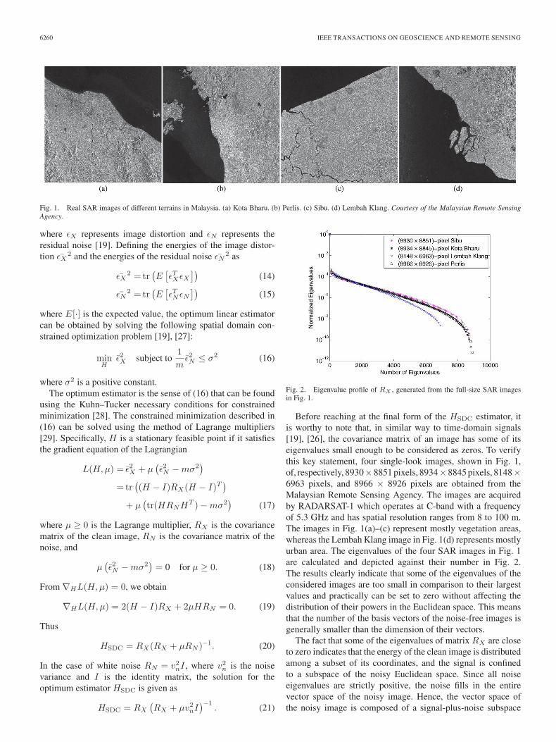
Fig. 1. Real SAR images of different terrains in Malaysia. (a) Kota Bharu. (b) Perlis. (c) Sibu. (d) Lembah Klang. Courtesy of the Malaysian Remote SensingAgency.
where εX represents image distortion and εN represents theresidual noise [19]. Defining the energies of the image distor-tion ε̄X
2 and the energies of the residual noise ε̄N2 as
ε̄X2 =tr
(E[εTXεX
])(14)
ε̄N2 =tr
(E[εTN εN
])(15)
where E[·] is the expected value, the optimum linear estimatorcan be obtained by solving the following spatial domain con-strained optimization problem [19], [27]:
minH
ε̄2X subject to1
mε̄2N ≤ σ2 (16)
where σ2 is a positive constant.The optimum estimator is the sense of (16) that can be found
using the Kuhn–Tucker necessary conditions for constrainedminimization [28]. The constrained minimization described in(16) can be solved using the method of Lagrange multipliers[29]. Specifically, H is a stationary feasible point if it satisfiesthe gradient equation of the Lagrangian
L(H,μ) = ε̄2X + μ(ε̄2N −mσ2
)=tr
((H − I)RX(H − I)T
)+ μ
(tr(HRNHT )−mσ2
)(17)
where μ ≥ 0 is the Lagrange multiplier, RX is the covariancematrix of the clean image, RN is the covariance matrix of thenoise, and
μ(ε̄2N −mσ2
)= 0 for μ ≥ 0. (18)
From ∇HL(H,μ) = 0, we obtain
∇HL(H,μ) = 2(H − I)RX + 2μHRN = 0. (19)
Thus
HSDC = RX(RX + μRN )−1. (20)
In the case of white noise RN = v2nI , where v2n is the noisevariance and I is the identity matrix, the solution for theoptimum estimator HSDC is given as
HSDC = RX
(RX + μv2nI
)−1. (21)
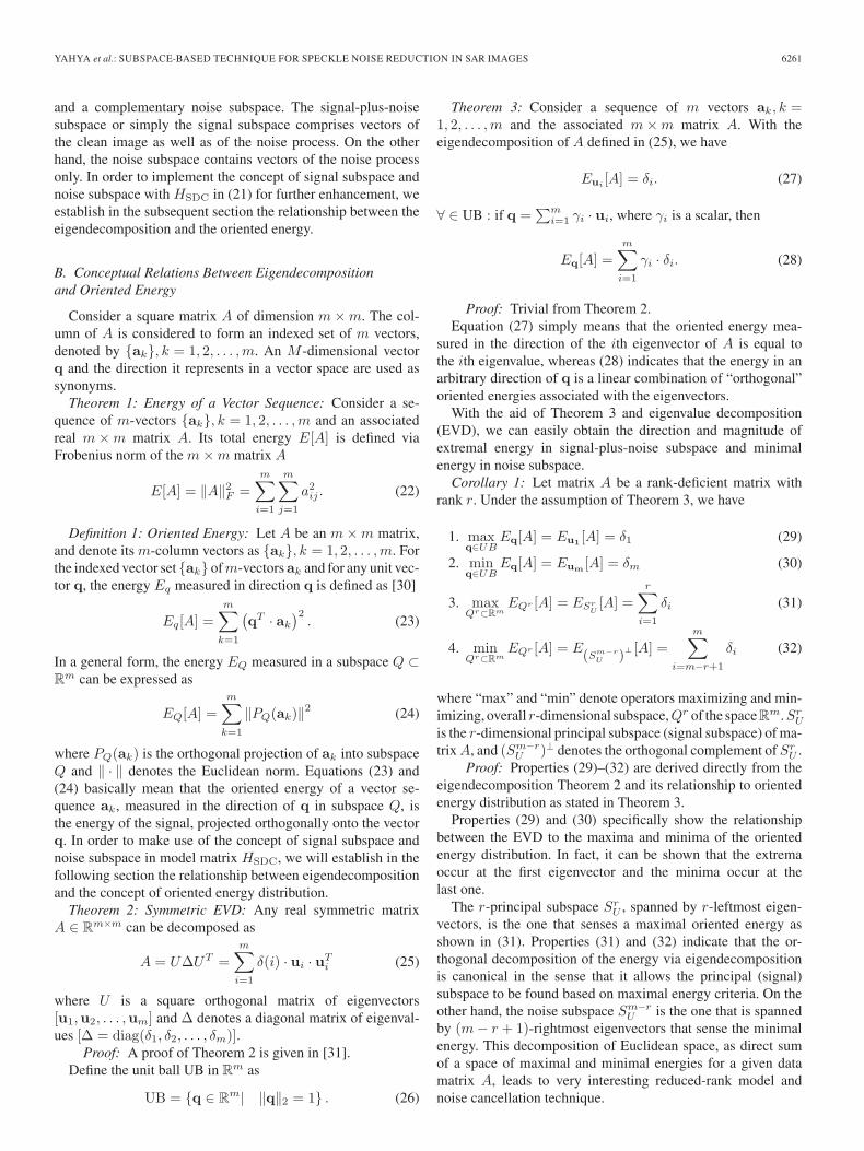
Fig. 2. Eigenvalue profile of RX , generated from the full-size SAR imagesin Fig. 1.
Before reaching at the final form of the HSDC estimator, itis worthy to note that, in similar way to time-domain signals[19], [26], the covariance matrix of an image has some of itseigenvalues small enough to be considered as zeros. To verifythis key statement, four single-look images, shown in Fig. 1,of, respectively, 8930×8851 pixels, 8934×8845 pixels, 8148×6963 pixels, and 8966 × 8926 pixels are obtained from theMalaysian Remote Sensing Agency. The images are acquiredby RADARSAT-1 which operates at C-band with a frequencyof 5.3 GHz and has spatial resolution ranges from 8 to 100 m.The images in Fig. 1(a)–(c) represent mostly vegetation areas,whereas the Lembah Klang image in Fig. 1(d) represents mostlyurban area. The eigenvalues of the four SAR images in Fig. 1are calculated and depicted against their number in Fig. 2.The results clearly indicate that some of the eigenvalues of theconsidered images are too small in comparison to their largestvalues and practically can be set to zero without affecting thedistribution of their powers in the Euclidean space. This meansthat the number of the basis vectors of the noise-free images isgenerally smaller than the dimension of their vectors.
The fact that some of the eigenvalues of matrix RX are closeto zero indicates that the energy of the clean image is distributedamong a subset of its coordinates, and the signal is confinedto a subspace of the noisy Euclidean space. Since all noiseeigenvalues are strictly positive, the noise fills in the entirevector space of the noisy image. Hence, the vector space ofthe noisy image is composed of a signal-plus-noise subspace
YAHYA et al.: SUBSPACE-BASED TECHNIQUE FOR SPECKLE NOISE REDUCTION IN SAR IMAGES 6261
and a complementary noise subspace. The signal-plus-noisesubspace or simply the signal subspace comprises vectors ofthe clean image as well as of the noise process. On the otherhand, the noise subspace contains vectors of the noise processonly. In order to implement the concept of signal subspace andnoise subspace with HSDC in (21) for further enhancement, weestablish in the subsequent section the relationship between theeigendecomposition and the oriented energy.
B. Conceptual Relations Between Eigendecompositionand Oriented Energy
Consider a square matrix A of dimension m×m. The col-umn of A is considered to form an indexed set of m vectors,denoted by {ak}, k = 1, 2, . . . ,m. An M -dimensional vectorq and the direction it represents in a vector space are used assynonyms.
Theorem 1: Energy of a Vector Sequence: Consider a se-quence of m-vectors {ak}, k = 1, 2, . . . ,m and an associatedreal m×m matrix A. Its total energy E[A] is defined viaFrobenius norm of the m×m matrix A
E[A] = ‖A‖2F =
m∑i=1
m∑j=1
a2ij . (22)
Definition 1: Oriented Energy: Let A be an m×m matrix,and denote its m-column vectors as {ak}, k = 1, 2, . . . ,m. Forthe indexed vector set {ak} ofm-vectorsak and for any unit vec-tor q, the energy Eq measured in direction q is defined as [30]
Eq[A] =
m∑k=1
(qT · ak
)2. (23)
In a general form, the energy EQ measured in a subspace Q ⊂R
m can be expressed as
EQ[A] =
m∑k=1
‖PQ(ak)‖2 (24)
where PQ(ak) is the orthogonal projection of ak into subspaceQ and ‖ · ‖ denotes the Euclidean norm. Equations (23) and(24) basically mean that the oriented energy of a vector se-quence ak, measured in the direction of q in subspace Q, isthe energy of the signal, projected orthogonally onto the vectorq. In order to make use of the concept of signal subspace andnoise subspace in model matrix HSDC, we will establish in thefollowing section the relationship between eigendecompositionand the concept of oriented energy distribution.
Theorem 2: Symmetric EVD: Any real symmetric matrixA ∈ R
m×m can be decomposed as
A = UΔUT =
m∑i=1
δ(i) · ui · uTi (25)
where U is a square orthogonal matrix of eigenvectors[u1,u2, . . . ,um] and Δ denotes a diagonal matrix of eigenval-ues [Δ = diag(δ1, δ2, . . . , δm)].
Proof: A proof of Theorem 2 is given in [31].Define the unit ball UB in R
m as
UB = {q ∈ Rm| ‖q‖2 = 1} . (26)
Theorem 3: Consider a sequence of m vectors ak, k =1, 2, . . . ,m and the associated m×m matrix A. With theeigendecomposition of A defined in (25), we have
Eui[A] = δi. (27)
∀ ∈ UB : if q =∑m
i=1 γi · ui, where γi is a scalar, then
Eq[A] =m∑i=1
γi · δi. (28)
Proof: Trivial from Theorem 2.Equation (27) simply means that the oriented energy mea-
sured in the direction of the ith eigenvector of A is equal tothe ith eigenvalue, whereas (28) indicates that the energy in anarbitrary direction of q is a linear combination of “orthogonal”oriented energies associated with the eigenvectors.
With the aid of Theorem 3 and eigenvalue decomposition(EVD), we can easily obtain the direction and magnitude ofextremal energy in signal-plus-noise subspace and minimalenergy in noise subspace.
Corollary 1: Let matrix A be a rank-deficient matrix withrank r. Under the assumption of Theorem 3, we have
1. maxq∈UB
Eq[A] = Eu1[A] = δ1 (29)
2. minq∈UB
Eq[A] = Eum[A] = δm (30)
3. maxQr⊂Rm
EQr [A] = ESrU[A] =
r∑i=1
δi (31)
4. minQr⊂Rm
EQr [A] = E(Sm−r
U )⊥ [A] =
m∑i=m−r+1
δi (32)
where “max” and “min” denote operators maximizing and min-imizing, overall r-dimensional subspace,Qr of the spaceRm.Sr
U
is the r-dimensional principal subspace (signal subspace) of ma-trix A, and (Sm−r
U )⊥ denotes the orthogonal complement of SrU .
Proof: Properties (29)–(32) are derived directly from theeigendecomposition Theorem 2 and its relationship to orientedenergy distribution as stated in Theorem 3.
Properties (29) and (30) specifically show the relationshipbetween the EVD to the maxima and minima of the orientedenergy distribution. In fact, it can be shown that the extremaoccur at the first eigenvector and the minima occur at thelast one.
The r-principal subspace SrU , spanned by r-leftmost eigen-
vectors, is the one that senses a maximal oriented energy asshown in (31). Properties (31) and (32) indicate that the or-thogonal decomposition of the energy via eigendecompositionis canonical in the sense that it allows the principal (signal)subspace to be found based on maximal energy criteria. On theother hand, the noise subspace Sm−r
U is the one that is spannedby (m− r + 1)-rightmost eigenvectors that sense the minimalenergy. This decomposition of Euclidean space, as direct sumof a space of maximal and minimal energies for a given datamatrix A, leads to very interesting reduced-rank model andnoise cancellation technique.
6262 IEEE TRANSACTIONS ON GEOSCIENCE AND REMOTE SENSING
C. Optimum Estimator Using Principal Subspace
Having established the link between the maximal orientedenergy and the signal subspace as well as between the minimalenergy and the noise subspace, we are in a position to improvethe form of HSDC in (21) by removing the noise subspace andestimating the clean image from the remaining signal subspace.Consider the covariance matrix of the clean image RX as a rankdeficient matrix with rank r. Assume matrix U ∈ R
m×m as theeigenvectors of RX . Let us partition U into r vectors that spanthe signal subspace and (m− r) vectors that span the noisesubspace. Using EVD, this can be expressed as
RX =UXΔXUTX
=(U1 U2)
(ΔX1 00 0
)(UT1
UT2
)(33)
where U1 is an (m× r)-matrix, U2 is an m× (m− r)-matrix,and ΔX1 = diag(δ1, δ2, . . . , δr). Since the noise is consideredto be white, the noise covariance matrix can be expressed asRN = v2nIm, and the eigenvectors U are unaffected by theconstant diagonal perturbation [26]. Using the effect of smallperturbation on data matrix, the eigendecomposition of RY isexpressed as
RY =UY ΔY UTY
=(U1 U2)
(ΔX1 + v2nIr 0
0 v2nIm−r
)(UT1
UT2
). (34)
From (33) and (34), it is clear that the eigenvectors for theclean and noisy covariance matrices are the same. On the otherhand, the eigenvalues of RY are equal to the sum of ΔX andnoise variance v2n; hence, ΔX can be estimated directly from(34) provided that the value of v2n is known. This results in thefollowing form for the linear estimator in (21):
HSDC = U1ΔX1
(ΔX1 + μv2nI
)−1UT1 (35)
where Δ(i)X = Δ
(i)Y − v2n. To implement (35) for HSDC, the
rank of the signal subspace r and the optimum value ofthe Langrage multiplier μ are considered a priori known. Inthe subsequent two sections, we discuss the optimum values ofr and μ.
D. Estimation of Noise Variance
In [32], Moor gives a detailed analysis on the validity of sin-gular value decomposition (SVD) in subspace-based methodsin dealing with additive white noise. One of the establishedalgebraic and geometric conditions is that there is a distinct gapbetween the smallest singular value of the signal subspace andthe largest singular value of the noise subspace. Theoretically,the last (n− r)-trailing end of the smallest singular is similarand equal to the noise standard deviation value. Thus, the noisevariance can be estimated as
v2n =1
n− r
n∑i=r+1
α2Y,i (36)
where αY,i is the ith singular value of the noisy image Y .
E. Rank Estimation of Matrix A
Consider that matrix A ∈ Rm×n represents an image, and it
is needed to find its best approximation in terms of a reduced-dimension matrix B. A commonly used method for such pur-pose is to approximate A with a matrix of lower rank. Themathematical formulation of the optimal rank-p approximationof A, under the Frobenius norm, is a problem of finding a lowerranked matrix B ∈ R
m×n with rank(B) = p such that
B = arg minrank(B)=p
‖A−B‖2F . (37)
Matrix B can be obtained by computing the SVD of A, as statedin the following theorem [31].
Theorem 4: Let the SVD of A ∈ Rm×n be
Am×n = Um×m · Sm×n · V Tn×n (38)
where U and V are real orthonormal, and the matrix
S = diag(α1, . . . , αr, 0, . . . , 0) (39)
where α1 ≥ α2 ≥ · · ·αr > αr+1 = · · · = αn = 0 and r =rank(A). Then
r∑i=p+1
α2i = min
rank(B)=p‖A−B‖2F , 1 ≤ p ≤ r. (40)
The minimum is achieved with B = bestp(A), where
bestp(A) = Up · diag(α1, . . . , αp) · V Tp . (41)
Here, Up and Vp are the matrices formed by the first p columnsof U and V , respectively.
This means that, for any approximation B of A, the term‖A−B‖F is the reconstruction error, and by Theorem 4, B =Up · diag(α1, . . . αp) · V T
p has the smallest reconstruction erroramong all of the rank-p approximations of A.
Using this approximation, each m-dimensional column aiof A can be approximated as ai ≈ Upa
Li , for some aLi ∈ R
m.Since Up has orthonormal columns∥∥Upa
Li − Upa
Lj
∥∥ =∥∥aLi − aLj
∥∥ (42)
which basically means that the Euclidean distance between twovectors is preserved under the orthogonal projection. It fol-lows that
‖ai − aj‖ ≈∥∥Upa
Li − Upa
Lj
∥∥ =∥∥aLi − aLj
∥∥ . (43)
Since each ai is approximated by UpaLi , where Up is com-
mon for every ai, hence we only need to store Up and {aLi }ni=1
for all approximation. With Up ∈ Rm×p and aLi ∈ R
p, fori = 1, . . . , n, it would require (mp+ np) scalars to store thereduced representations. In this case, for original image matrixA of size m× n, the compression ratio Cr using the rank-papproximation is [33], [34]
Cr =mn
(m+ n)p. (44)
Now, let us consider the problem of finding the rank of anoisy image Y that follows the additive noise model in (11).
YAHYA et al.: SUBSPACE-BASED TECHNIQUE FOR SPECKLE NOISE REDUCTION IN SAR IMAGES 6263
Fundamentally, the clean matrix X has a reduced rank r ≤min(m,n), whereas the noise matrix N has full rank. Thesingular values of Y are given by
S = diag (α1, . . . , αn) (45)
where α1 ≥ α2 ≥ · · ·αr > αr+1 ≥ · · · ≥ αn ≥ 0 and (αr+1,. . . , αn) are usually small but not necessarily zero. One ap-proach to estimate the rank r of the matrix Y from the computedsingular values is to have a tolerance τ and a convention thatY has “numerical” rank r if its singular values satisfy thefollowing criteria [31]:
α1 ≥ α2 ≥ · · ·αr > τ ≥ αr+1 ≥ · · · ≥ αn. (46)
Different statistical models were proposed for the selection ofthe threshold bounds τ . Among the best-known models are thefinite precision model, the i.i.d. random model, and the columnrandom model [35]. In this paper, the selected threshold boundis based on the i.i.d. random model given by [35]
c ≤ τ ≤√(mn)c (47)
where 2vn ≤ c ≤ 2.6vn and vn is the standard deviation of thenoise. The threshold bound in (47) is derived using the pertur-bation theory of singular values and a statistical significancetest. Based on (47), the obtained threshold bound is a functionof matrix dimension, noise variance, and predefined statisticallevel of significance.
F. Optimum Value of the Lagrange Multiplier
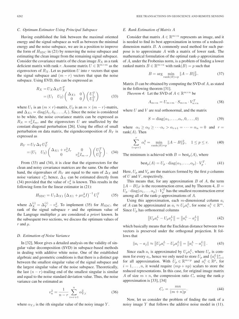
To find the best μ value for SDC, a mosaic image composedof synthetic patterns, specimens from Broadatz texture set, andtwo optical remote sensing images is created. The image ismade up of four quarters, each of 256 × 256 pixels, and isshown in Fig. 3(a). The first quarter represents syntheticallycreated homogenous regions, the second quarter is an opticalimage showing a mountainous area, the third quarter is anotheroptical image showing an airport area, and the fourth quarteris taken from Broadatz texture set. The test image is corruptedwith speckle noise of variance that extends from 0.02 to 0.2,and the SDC is run with μ ranging between 10 and 300. Thesignal-to-noise ratio (SNR) value calculated as
SNRdB = 10 log10v̄2X
MSE(48)
where MSE represents the mean-square error, given by
MSE =1
mn
m∑i=1
n∑j=1
(X(i, j)− Y (i, j))2 (49)
is used to indicate the denoising effect of the SDC. The resultsare shown in Fig. 3(b).
The results in Fig. 3(b) show that the SDC is not too sensitiveto the selected value of the Lagrange multiplier. In particular,the despeckle effect of the SDC, measured in terms of the SNR,shows improvement by only 1-1.5 dB, for the different values ofthe noise variance, as the Lagrange multiplier varies from 5 to
Fig. 3. (a) Mosaic test image. (b) SNR of the mosaic image in (a) obtained atdifferent μ values.
300. In general, the results in Fig. 3(b) show better SNR valuesfor higher values of the Lagrange multiplier. However, it shouldbe noted that the high value of μ may result in oversmoothedimages and may cause loss of details. Consequently, the rule ofselecting μ is that, for noise variance less than 0.06, μ shouldbe selected within the range from 50 to 100 and, with noisevariance greater than 0.06, it should be selected around 200.
G. Implementation of Signal Subspace Approach forUncorrelated Speckle Noise
1) Apply the homomorphic transformation to the noisy im-age Yl = log(G).
2) Estimate the noise variance v2n.3) Compute the dimension of signal subspace r.4) Using the estimated r in step 3, apply eigendecompo-
sition on RYl; then, extract the basis vectors of signal sub-
space U1 and their related eigenvalues Δ(i)X = Δ
(i)Y − v2n.
5) Select μ according to the rule in Section III-F; then,compute the optimum linear estimator
HSDC = U1ΔX1
(ΔX1 + μv2nI
)−1UT1 . (50)
6) Compute the clean image X̂l = HSDC · Yl.
6264 IEEE TRANSACTIONS ON GEOSCIENCE AND REMOTE SENSING
7) Reverse the homomorphic effect by taking the exponen-tial of X̂l as follows:
X̂ = 10X̂l . (51)
8) Apply bias adjustment according to Section II-A.
IV. RESULTS AND DISCUSSIONS
This section is divided into two parts. In the first part, theperformance of the SDC as a function of the size of the image,as well as its capability in representing real SAR images,is investigated. In the second part, the performance of theproposed SDC technique is compared with both Lee [4] and thehomomorphic wavelet filter [20], [21] using synthetic imagesand real SAR images. Lee filter is implemented with 7 × 7window size, and the homomorphic wavelet is used with theDaubechies length-eight filter and a 7 × 7 window. The SDCis implemented as in Section III-G. The rank values of thedifferent images are calculated using the method outlined inSection III-E, and the Lagrange multiplier is selected usingthe rule set in Section III-F. The noise variance is estimatedusing (36).
A. Performance of SDC With the Size of the Image
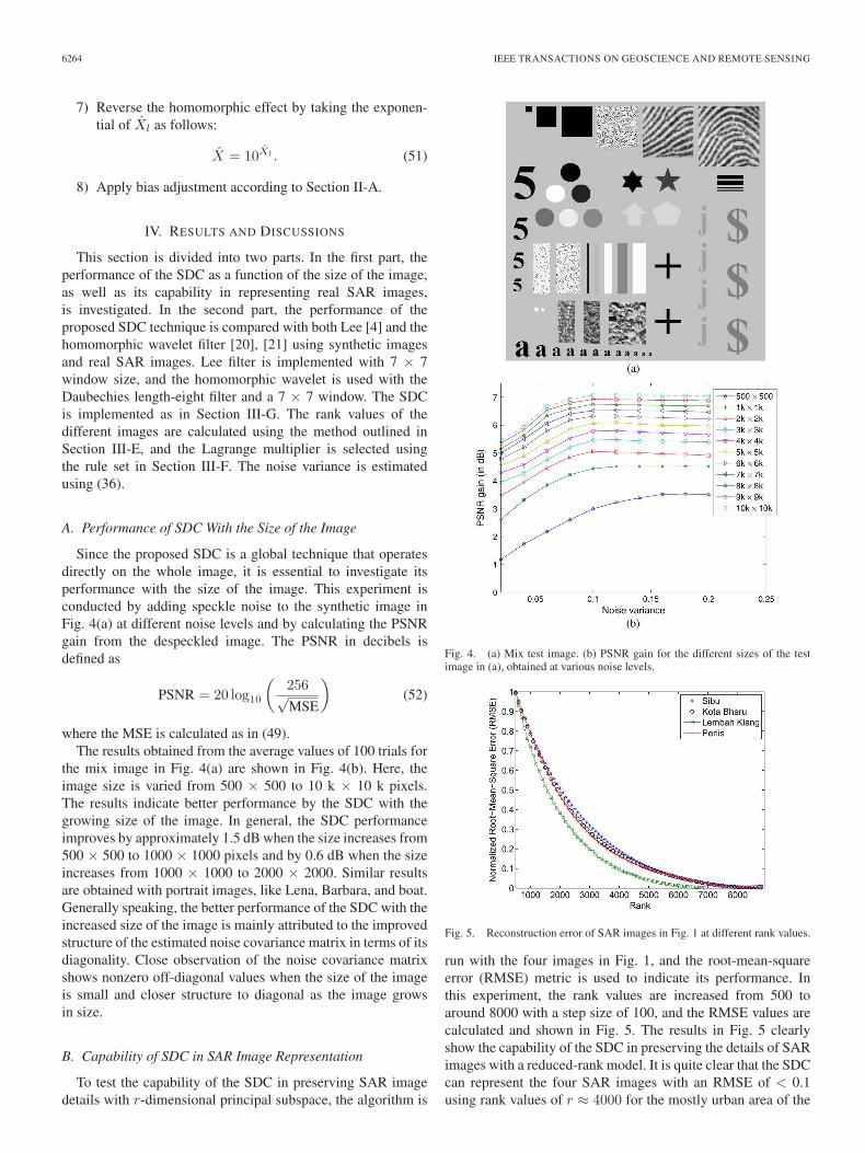
Since the proposed SDC is a global technique that operatesdirectly on the whole image, it is essential to investigate itsperformance with the size of the image. This experiment isconducted by adding speckle noise to the synthetic image inFig. 4(a) at different noise levels and by calculating the PSNRgain from the despeckled image. The PSNR in decibels isdefined as
PSNR = 20 log10
(256√MSE
)(52)
where the MSE is calculated as in (49).The results obtained from the average values of 100 trials for
the mix image in Fig. 4(a) are shown in Fig. 4(b). Here, theimage size is varied from 500 × 500 to 10 k × 10 k pixels.The results indicate better performance by the SDC with thegrowing size of the image. In general, the SDC performanceimproves by approximately 1.5 dB when the size increases from500 × 500 to 1000 × 1000 pixels and by 0.6 dB when the sizeincreases from 1000 × 1000 to 2000 × 2000. Similar resultsare obtained with portrait images, like Lena, Barbara, and boat.Generally speaking, the better performance of the SDC with theincreased size of the image is mainly attributed to the improvedstructure of the estimated noise covariance matrix in terms of itsdiagonality. Close observation of the noise covariance matrixshows nonzero off-diagonal values when the size of the imageis small and closer structure to diagonal as the image growsin size.
B. Capability of SDC in SAR Image Representation
To test the capability of the SDC in preserving SAR imagedetails with r-dimensional principal subspace, the algorithm is
Fig. 4. (a) Mix test image. (b) PSNR gain for the different sizes of the testimage in (a), obtained at various noise levels.
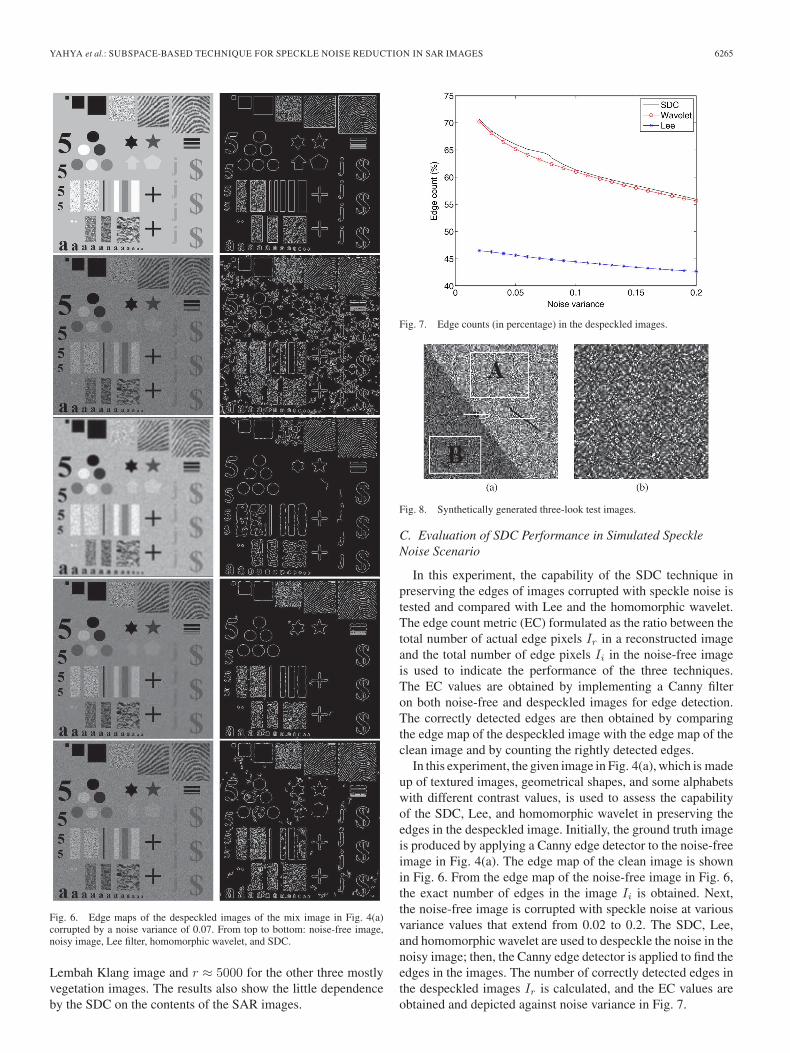
Fig. 5. Reconstruction error of SAR images in Fig. 1 at different rank values.
run with the four images in Fig. 1, and the root-mean-squareerror (RMSE) metric is used to indicate its performance. Inthis experiment, the rank values are increased from 500 toaround 8000 with a step size of 100, and the RMSE values arecalculated and shown in Fig. 5. The results in Fig. 5 clearlyshow the capability of the SDC in preserving the details of SARimages with a reduced-rank model. It is quite clear that the SDCcan represent the four SAR images with an RMSE of < 0.1using rank values of r ≈ 4000 for the mostly urban area of the
YAHYA et al.: SUBSPACE-BASED TECHNIQUE FOR SPECKLE NOISE REDUCTION IN SAR IMAGES 6265
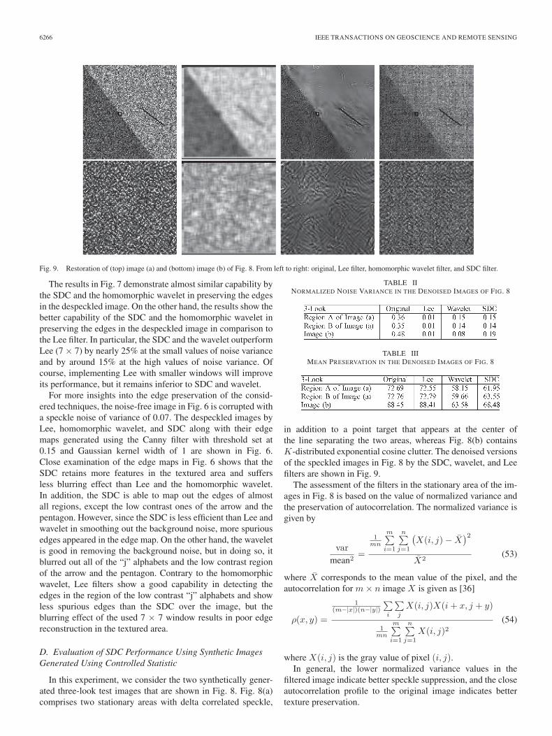
Fig. 6. Edge maps of the despeckled images of the mix image in Fig. 4(a)corrupted by a noise variance of 0.07. From top to bottom: noise-free image,noisy image, Lee filter, homomorphic wavelet, and SDC.
Lembah Klang image and r ≈ 5000 for the other three mostlyvegetation images. The results also show the little dependenceby the SDC on the contents of the SAR images.
Fig. 7. Edge counts (in percentage) in the despeckled images.
Fig. 8. Synthetically generated three-look test images.
C. Evaluation of SDC Performance in Simulated SpeckleNoise Scenario
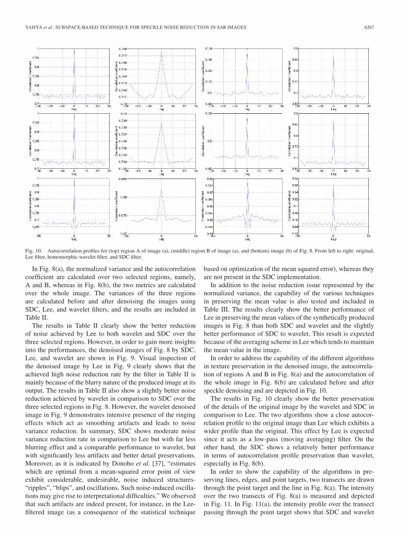
In this experiment, the capability of the SDC technique inpreserving the edges of images corrupted with speckle noise istested and compared with Lee and the homomorphic wavelet.The edge count metric (EC) formulated as the ratio between thetotal number of actual edge pixels Ir in a reconstructed imageand the total number of edge pixels Ii in the noise-free imageis used to indicate the performance of the three techniques.The EC values are obtained by implementing a Canny filteron both noise-free and despeckled images for edge detection.The correctly detected edges are then obtained by comparingthe edge map of the despeckled image with the edge map of theclean image and by counting the rightly detected edges.
In this experiment, the given image in Fig. 4(a), which is madeup of textured images, geometrical shapes, and some alphabetswith different contrast values, is used to assess the capabilityof the SDC, Lee, and homomorphic wavelet in preserving theedges in the despeckled image. Initially, the ground truth imageis produced by applying a Canny edge detector to the noise-freeimage in Fig. 4(a). The edge map of the clean image is shownin Fig. 6. From the edge map of the noise-free image in Fig. 6,the exact number of edges in the image Ii is obtained. Next,the noise-free image is corrupted with speckle noise at variousvariance values that extend from 0.02 to 0.2. The SDC, Lee,and homomorphic wavelet are used to despeckle the noise in thenoisy image; then, the Canny edge detector is applied to find theedges in the images. The number of correctly detected edges inthe despeckled images Ir is calculated, and the EC values areobtained and depicted against noise variance in Fig. 7.
6266 IEEE TRANSACTIONS ON GEOSCIENCE AND REMOTE SENSING
Fig. 9. Restoration of (top) image (a) and (bottom) image (b) of Fig. 8. From left to right: original, Lee filter, homomorphic wavelet filter, and SDC filter.
The results in Fig. 7 demonstrate almost similar capability bythe SDC and the homomorphic wavelet in preserving the edgesin the despeckled image. On the other hand, the results show thebetter capability of the SDC and the homomorphic wavelet inpreserving the edges in the despeckled image in comparison tothe Lee filter. In particular, the SDC and the wavelet outperformLee (7 × 7) by nearly 25% at the small values of noise varianceand by around 15% at the high values of noise variance. Ofcourse, implementing Lee with smaller windows will improveits performance, but it remains inferior to SDC and wavelet.
For more insights into the edge preservation of the consid-ered techniques, the noise-free image in Fig. 6 is corrupted witha speckle noise of variance of 0.07. The despeckled images byLee, homomorphic wavelet, and SDC along with their edgemaps generated using the Canny filter with threshold set at0.15 and Gaussian kernel width of 1 are shown in Fig. 6.Close examination of the edge maps in Fig. 6 shows that theSDC retains more features in the textured area and suffersless blurring effect than Lee and the homomorphic wavelet.In addition, the SDC is able to map out the edges of almostall regions, except the low contrast ones of the arrow and thepentagon. However, since the SDC is less efficient than Lee andwavelet in smoothing out the background noise, more spuriousedges appeared in the edge map. On the other hand, the waveletis good in removing the background noise, but in doing so, itblurred out all of the “j” alphabets and the low contrast regionof the arrow and the pentagon. Contrary to the homomorphicwavelet, Lee filters show a good capability in detecting theedges in the region of the low contrast “j” alphabets and showless spurious edges than the SDC over the image, but theblurring effect of the used 7 × 7 window results in poor edgereconstruction in the textured area.
D. Evaluation of SDC Performance Using Synthetic ImagesGenerated Using Controlled Statistic
In this experiment, we consider the two synthetically gener-ated three-look test images that are shown in Fig. 8. Fig. 8(a)comprises two stationary areas with delta correlated speckle,
TABLE IINORMALIZED NOISE VARIANCE IN THE DENOISED IMAGES OF FIG. 8
TABLE IIIMEAN PRESERVATION IN THE DENOISED IMAGES OF FIG. 8
in addition to a point target that appears at the center ofthe line separating the two areas, whereas Fig. 8(b) containsK-distributed exponential cosine clutter. The denoised versionsof the speckled images in Fig. 8 by the SDC, wavelet, and Leefilters are shown in Fig. 9.
The assessment of the filters in the stationary area of the im-ages in Fig. 8 is based on the value of normalized variance andthe preservation of autocorrelation. The normalized variance isgiven by
var
mean2=
1mn
m∑i=1
n∑j=1
(X(i, j)− X̄
)2X̄2
(53)
where X̄ corresponds to the mean value of the pixel, and theautocorrelation for m× n image X is given as [36]
ρ(x, y) =
1(m−|x|)(n−|y|)
∑i
∑j
X(i, j)X(i+ x, j + y)
1mn
m∑i=1
n∑j=1
X(i, j)2(54)
where X(i, j) is the gray value of pixel (i, j).In general, the lower normalized variance values in the
filtered image indicate better speckle suppression, and the closeautocorrelation profile to the original image indicates bettertexture preservation.
YAHYA et al.: SUBSPACE-BASED TECHNIQUE FOR SPECKLE NOISE REDUCTION IN SAR IMAGES 6267
Fig. 10. Autocorrelation profiles for (top) region A of image (a), (middle) region B of image (a), and (bottom) image (b) of Fig. 8. From left to right: original,Lee filter, homomorphic wavelet filter, and SDC filter.
In Fig. 8(a), the normalized variance and the autocorrelationcoefficient are calculated over two selected regions, namely,A and B, whereas in Fig. 8(b), the two metrics are calculatedover the whole image. The variances of the three regionsare calculated before and after denoising the images usingSDC, Lee, and wavelet filters, and the results are included inTable II.
The results in Table II clearly show the better reductionof noise achieved by Lee to both wavelet and SDC over thethree selected regions. However, in order to gain more insightsinto the performances, the denoised images of Fig. 8 by SDC,Lee, and wavelet are shown in Fig. 9. Visual inspection ofthe denoised image by Lee in Fig. 9 clearly shows that theachieved high noise reduction rate by the filter in Table II ismainly because of the blurry nature of the produced image at itsoutput. The results in Table II also show a slightly better noisereduction achieved by wavelet in comparison to SDC over thethree selected regions in Fig. 8. However, the wavelet denoisedimage in Fig. 9 demonstrates intensive presence of the ringingeffects which act as smoothing artifacts and leads to noisevariance reduction. In summary, SDC shows moderate noisevariance reduction rate in comparison to Lee but with far lessblurring effect and a comparable performance to wavelet, butwith significantly less artifacts and better detail preservations.Moreover, as it is indicated by Donoho et al. [37], “estimateswhich are optimal from a mean-squared error point of viewexhibit considerable, undesirable, noise induced structures-“ripples”, “blips”, and oscillations. Such noise-induced oscilla-tions may give rise to interpretational difficulties.” We observedthat such artifacts are indeed present, for instance, in the Lee-filtered image (as a consequence of the statistical technique
based on optimization of the mean squared error), whereas theyare not present in the SDC implementation.
In addition to the noise reduction issue represented by thenormalized variance, the capability of the various techniquesin preserving the mean value is also tested and included inTable III. The results clearly show the better performance ofLee in preserving the mean values of the synthetically producedimages in Fig. 8 than both SDC and wavelet and the slightlybetter performance of SDC to wavelet. This result is expectedbecause of the averaging scheme in Lee which tends to maintainthe mean value in the image.
In order to address the capability of the different algorithmsin texture preservation in the denoised image, the autocorrela-tion of regions A and B in Fig. 8(a) and the autocorrelation ofthe whole image in Fig. 8(b) are calculated before and afterspeckle denoising and are depicted in Fig. 10.
The results in Fig. 10 clearly show the better preservationof the details of the original image by the wavelet and SDC incomparison to Lee. The two algorithms show a close autocor-relation profile to the original image than Lee which exhibits awider profile than the original. This effect by Lee is expectedsince it acts as a low-pass (moving averaging) filter. On theother hand, the SDC shows a relatively better performancein terms of autocorrelation profile preservation than wavelet,especially in Fig. 8(b).
In order to show the capability of the algorithms in pre-serving lines, edges, and point targets, two transects are drawnthrough the point target and the line in Fig. 8(a). The intensityover the two transects of Fig. 8(a) is measured and depictedin Fig. 11. In Fig. 11(a), the intensity profile over the transectpassing through the point target shows that SDC and wavelet
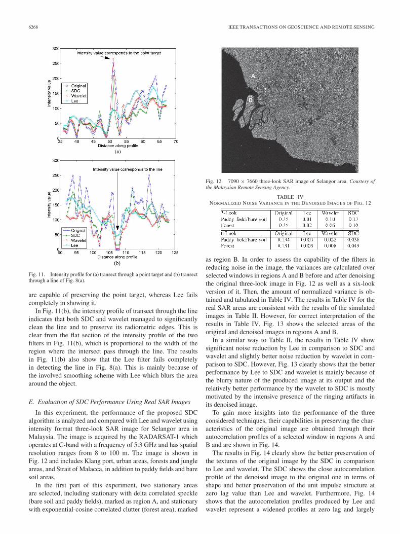
6268 IEEE TRANSACTIONS ON GEOSCIENCE AND REMOTE SENSING
Fig. 11. Intensity profile for (a) transect through a point target and (b) transectthrough a line of Fig. 8(a).
are capable of preserving the point target, whereas Lee failscompletely in showing it.
In Fig. 11(b), the intensity profile of transect through the lineindicates that both SDC and wavelet managed to significantlyclean the line and to preserve its radiometric edges. This isclear from the flat section of the intensity profile of the twofilters in Fig. 11(b), which is proportional to the width of theregion where the intersect pass through the line. The resultsin Fig. 11(b) also show that the Lee filter fails completelyin detecting the line in Fig. 8(a). This is mainly because ofthe involved smoothing scheme with Lee which blurs the areaaround the object.
E. Evaluation of SDC Performance Using Real SAR Images
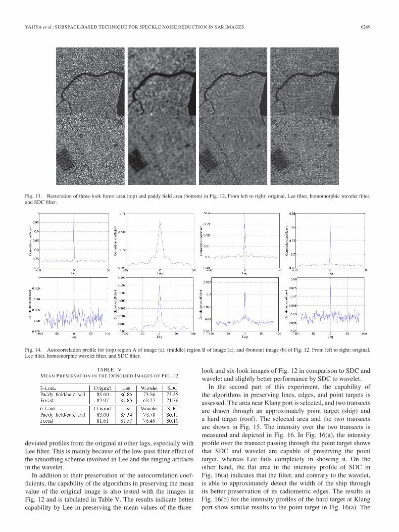
In this experiment, the performance of the proposed SDCalgorithm is analyzed and compared with Lee and wavelet usingintensity format three-look SAR image for Selangor area inMalaysia. The image is acquired by the RADARSAT-1 whichoperates at C-band with a frequency of 5.3 GHz and has spatialresolution ranges from 8 to 100 m. The image is shown inFig. 12 and includes Klang port, urban areas, forests and jungleareas, and Strait of Malacca, in addition to paddy fields and baresoil areas.
In the first part of this experiment, two stationary areasare selected, including stationary with delta correlated speckle(bare soil and paddy fields), marked as region A, and stationarywith exponential-cosine correlated clutter (forest area), marked
Fig. 12. 7090 × 7660 three-look SAR image of Selangor area. Courtesy ofthe Malaysian Remote Sensing Agency.
TABLE IVNORMALIZED NOISE VARIANCE IN THE DENOISED IMAGES OF FIG. 12
as region B. In order to assess the capability of the filters inreducing noise in the image, the variances are calculated overselected windows in regions A and B before and after denoisingthe original three-look image in Fig. 12 as well as a six-lookversion of it. Then, the amount of normalized variance is ob-tained and tabulated in Table IV. The results in Table IV for thereal SAR areas are consistent with the results of the simulatedimages in Table II. However, for correct interpretation of theresults in Table IV, Fig. 13 shows the selected areas of theoriginal and denoised images in regions A and B.
In a similar way to Table II, the results in Table IV showsignificant noise reduction by Lee in comparison to SDC andwavelet and slightly better noise reduction by wavelet in com-parison to SDC. However, Fig. 13 clearly shows that the betterperformance by Lee to SDC and wavelet is mainly because ofthe blurry nature of the produced image at its output and therelatively better performance by the wavelet to SDC is mostlymotivated by the intensive presence of the ringing artifacts inits denoised image.
To gain more insights into the performance of the threeconsidered techniques, their capabilities in preserving the char-acteristics of the original image are obtained through theirautocorrelation profiles of a selected window in regions A andB and are shown in Fig. 14.
The results in Fig. 14 clearly show the better preservation ofthe textures of the original image by the SDC in comparisonto Lee and wavelet. The SDC shows the close autocorrelationprofile of the denoised image to the original one in terms ofshape and better preservation of the unit impulse structure atzero lag value than Lee and wavelet. Furthermore, Fig. 14shows that the autocorrelation profiles produced by Lee andwavelet represent a widened profiles at zero lag and largely
YAHYA et al.: SUBSPACE-BASED TECHNIQUE FOR SPECKLE NOISE REDUCTION IN SAR IMAGES 6269
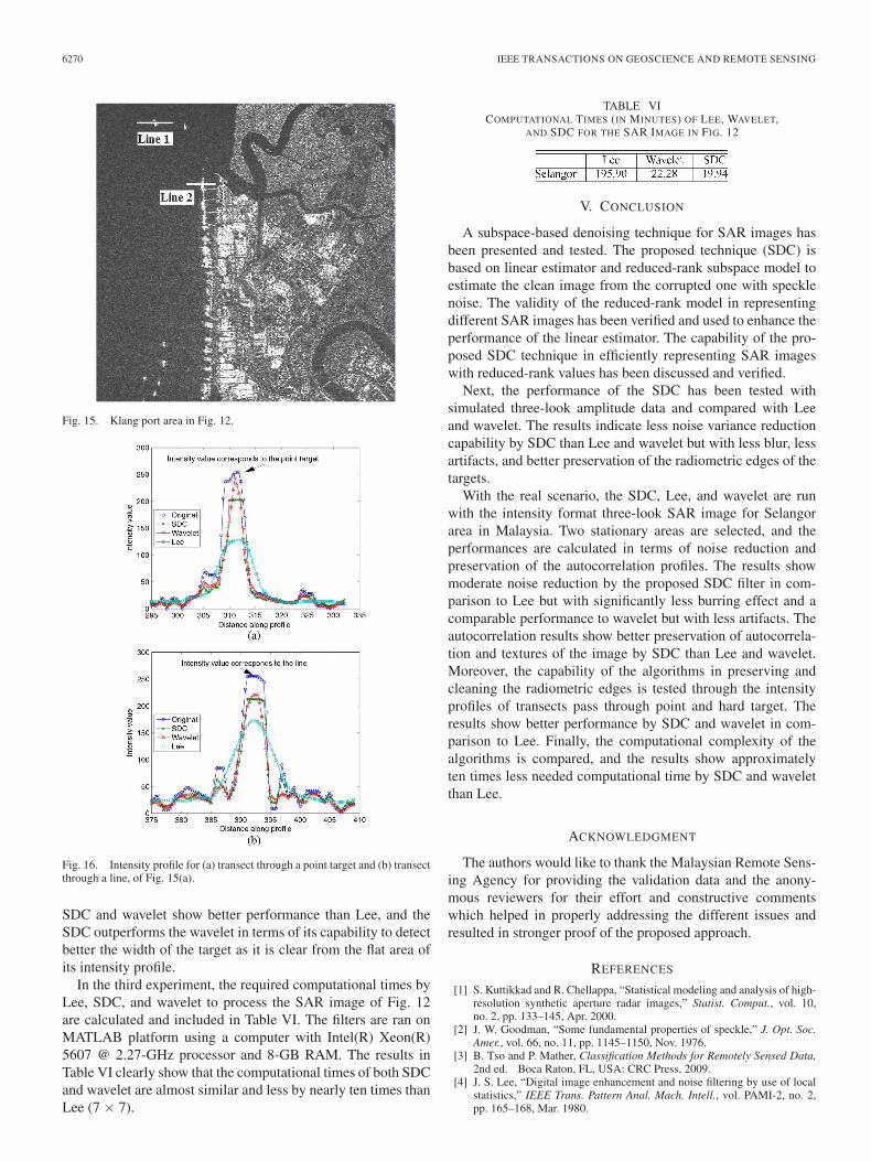
Fig. 13. Restoration of three-look forest area (top) and paddy field area (bottom) in Fig. 12. From left to right: original, Lee filter, homomorphic wavelet filter,and SDC filter.
Fig. 14. Autocorrelation profile for (top) region A of image (a), (middle) region B of image (a), and (bottom) image (b) of Fig. 12. From left to right: original,Lee filter, homomorphic wavelet filter, and SDC filter.
TABLE VMEAN PRESERVATION IN THE DENOISED IMAGES OF FIG. 12
deviated profiles from the original at other lags, especially withLee filter. This is mainly because of the low-pass filter effect ofthe smoothing scheme involved in Lee and the ringing artifactsin the wavelet.
In addition to their preservation of the autocorrelation coef-ficients, the capability of the algorithms in preserving the meanvalue of the original image is also tested with the images inFig. 12 and is tabulated in Table V. The results indicate bettercapability by Lee in preserving the mean values of the three-
look and six-look images of Fig. 12 in comparison to SDC andwavelet and slightly better performance by SDC to wavelet.
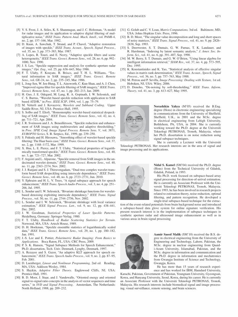
In the second part of this experiment, the capability ofthe algorithms in preserving lines, edges, and point targets isassessed. The area near Klang port is selected, and two transectsare drawn through an approximately point target (ship) anda hard target (roof). The selected area and the two transectsare shown in Fig. 15. The intensity over the two transects ismeasured and depicted in Fig. 16. In Fig. 16(a), the intensityprofile over the transect passing through the point target showsthat SDC and wavelet are capable of preserving the pointtarget, whereas Lee fails completely in showing it. On theother hand, the flat area in the intensity profile of SDC inFig. 16(a) indicates that the filter, and contrary to the wavelet,is able to approximately detect the width of the ship throughits better preservation of its radiometric edges. The results inFig. 16(b) for the intensity profiles of the hard target at Klangport show similar results to the point target in Fig. 16(a). The
6270 IEEE TRANSACTIONS ON GEOSCIENCE AND REMOTE SENSING
Fig. 15. Klang port area in Fig. 12.
Fig. 16. Intensity profile for (a) transect through a point target and (b) transectthrough a line, of Fig. 15(a).
SDC and wavelet show better performance than Lee, and theSDC outperforms the wavelet in terms of its capability to detectbetter the width of the target as it is clear from the flat area ofits intensity profile.
In the third experiment, the required computational times byLee, SDC, and wavelet to process the SAR image of Fig. 12are calculated and included in Table VI. The filters are ran onMATLAB platform using a computer with Intel(R) Xeon(R)5607 @ 2.27-GHz processor and 8-GB RAM. The results inTable VI clearly show that the computational times of both SDCand wavelet are almost similar and less by nearly ten times thanLee (7 × 7).
TABLE VICOMPUTATIONAL TIMES (IN MINUTES) OF LEE, WAVELET,
AND SDC FOR THE SAR IMAGE IN FIG. 12
V. CONCLUSION
A subspace-based denoising technique for SAR images hasbeen presented and tested. The proposed technique (SDC) isbased on linear estimator and reduced-rank subspace model toestimate the clean image from the corrupted one with specklenoise. The validity of the reduced-rank model in representingdifferent SAR images has been verified and used to enhance theperformance of the linear estimator. The capability of the pro-posed SDC technique in efficiently representing SAR imageswith reduced-rank values has been discussed and verified.
Next, the performance of the SDC has been tested withsimulated three-look amplitude data and compared with Leeand wavelet. The results indicate less noise variance reductioncapability by SDC than Lee and wavelet but with less blur, lessartifacts, and better preservation of the radiometric edges of thetargets.
With the real scenario, the SDC, Lee, and wavelet are runwith the intensity format three-look SAR image for Selangorarea in Malaysia. Two stationary areas are selected, and theperformances are calculated in terms of noise reduction andpreservation of the autocorrelation profiles. The results showmoderate noise reduction by the proposed SDC filter in com-parison to Lee but with significantly less burring effect and acomparable performance to wavelet but with less artifacts. Theautocorrelation results show better preservation of autocorrela-tion and textures of the image by SDC than Lee and wavelet.Moreover, the capability of the algorithms in preserving andcleaning the radiometric edges is tested through the intensityprofiles of transects pass through point and hard target. Theresults show better performance by SDC and wavelet in com-parison to Lee. Finally, the computational complexity of thealgorithms is compared, and the results show approximatelyten times less needed computational time by SDC and waveletthan Lee.
ACKNOWLEDGMENT
The authors would like to thank the Malaysian Remote Sens-ing Agency for providing the validation data and the anony-mous reviewers for their effort and constructive commentswhich helped in properly addressing the different issues andresulted in stronger proof of the proposed approach.
REFERENCES
[1] S. Kuttikkad and R. Chellappa, “Statistical modeling and analysis of high-resolution synthetic aperture radar images,” Statist. Comput., vol. 10,no. 2, pp. 133–145, Apr. 2000.
[2] J. W. Goodman, “Some fundamental properties of speckle,” J. Opt. Soc.Amer., vol. 66, no. 11, pp. 1145–1150, Nov. 1976.
[3] B. Tso and P. Mather, Classification Methods for Remotely Sensed Data,2nd ed. Boca Raton, FL, USA: CRC Press, 2009.
[4] J. S. Lee, “Digital image enhancement and noise filtering by use of localstatistics,” IEEE Trans. Pattern Anal. Mach. Intell., vol. PAMI-2, no. 2,pp. 165–168, Mar. 1980.
YAHYA et al.: SUBSPACE-BASED TECHNIQUE FOR SPECKLE NOISE REDUCTION IN SAR IMAGES 6271
[5] V. S. Frost, J. A. Stiles, K. S. Shanmugan, and J. C. Holtzman, “A modelfor radar images and its application to adaptive digital filtering of mul-tiplicative noise,” IEEE Trans. Pattern Anal. Mach. Intell., vol. PAMI-4,no. 2, pp. 157–166, Mar. 1982.
[6] D. Kuan, A. Sawchuk, T. Strand, and P. Chavel, “Adaptive restorationof images with speckle,” IEEE Trans. Acoust., Speech, Signal Process.,vol. 35, no. 3, pp. 373–383, Mar. 1987.
[7] A. Lopes, R. Touzi, and E. Nezry, “Adaptive speckle filters and sceneheterogeneity,” IEEE Trans. Geosci. Remote Sens., vol. 28, no. 6, pp. 992–1000, Nov. 1990.
[8] J. S. Lee, “Speckle suppression and analysis for synthetic aperture radarimages,” Opt. Eng., vol. 25, pp. 636–643, May 1986.
[9] F. T. Ulaby, F. Kouyate, B. Brisco, and T. H. L. Williams, “Tex-tural information in SAR images,” IEEE Trans. Geosci. RemoteSens., vol. GE-24, no. 2, pp. 235–245, Mar. 1986.
[10] L. Jong-Sen, W. Jen-Hung, T. L. Ainsworth, C. Kun-Shan, and A. J. Chen,“Improved sigma filter for speckle filtering of SAR imagery,” IEEE Trans.Geosci. Remote Sens., vol. 47, no. 1, pp. 202–213, Jan. 2009.
[11] H. Guo, J. E. Odegard, M. Lang, R. A. Gopinath, I. W. Selesnick, andC. S. Burrus, “Wavelet based speckle reduction with application to SARbased ATD/R,” in Proc. IEEE ICIP, 1994, vol. 1, pp. 75–79.
[12] M. Vetterli and J. Kovacevic, Wavelets and Subband Coding. UpperSaddle River, NJ, USA: Prentice-Hall, 1995.
[13] S. Solbo and T. Eltoft, “Homomorphic wavelet-based statistical despeck-ling of SAR images,” IEEE Trans. Geosci. Remote Sens., vol. 42, no. 4,pp. 711–721, Apr. 2004.
[14] J. R. Sveinsson and J. A. Benediktsson, “Speckle reduction and enhance-ment of SAR images using multiwavelets and adaptive thresholding,”in Proc. SPIE Conf. Image Signal Process. Remote Sens. V , vol. 3871,EUROPTO Series, S. B. Serpico, Ed., 1999, pp. 239–250.
[15] S. Fukuda and H. Hirosawa, “Smoothing effect of wavelet-based specklefiltering: The Haar basis case,” IEEE Trans. Geosci. Remote Sens., vol. 37,no. 2, pp. 1168–1172, Mar. 1999.
[16] X. Hua, L. E. Pierce, and F. T. Ulaby, “Statistical properties of logarith-mically transformed speckle,” IEEE Trans. Geosci. Remote Sens., vol. 40,no. 3, pp. 721–727, Mar. 2002.
[17] F. Argenti and L. Alparone, “Speckle removal from SAR images in the un-decimated wavelet domain,” IEEE Trans. Geosci. Remote Sens., vol. 40,no. 11, pp. 2363–2374, Nov. 2002.
[18] J. J. Ranjani and S. J. Thiruvengadam, “Dual-tree complex wavelet trans-form based SAR despeckling using interscale dependence,” IEEE Trans.Geosci. Remote Sens., vol. 48, no. 6, pp. 2723–2731, Jun. 2010.
[19] Y. Ephraim and H. L. V. Trees, “A signal subspace approach for speechenhancement,” IEEE Trans. Speech Audio Process., vol. 3, no. 4, pp. 251–266, Jul. 1995.
[20] L. Sendur and I. W. Selesnick, “Bivariate shrinkage functions for wavelet-based denoising exploiting interscale dependency,” IEEE Trans. SignalProcess., vol. 50, no. 11, pp. 2744–2756, Nov. 2002.
[21] L. Sendur and I. W. Selesnick, “Bivariate shrinkage with local varianceestimation,” IEEE Signal Process. Lett., vol. 9, no. 12, pp. 438–441,Dec. 2002.
[22] J. W. Goodman, Statistical Properties of Laser Speckle Patterns.Heidelberg, Germany: Springer-Verlag, 1980.
[23] F. T. Ulaby, Handbook of Radar Scattering Statistics for Terrain.Norwood, MA, USA: Artech House, 1989.
[24] D. H. Hoekman, “Speckle ensemble statistics of logarithmically scaleddata,” IEEE Trans. Geosci. Remote Sens., vol. 29, no. 1, pp. 180–182,Jan. 1991.
[25] J.-S. Lee and E. Pottier, Polarimetric Radar Imaging: From Basics toApplications. Boca Raton, FL, USA: CRC Press, 2009.
[26] P. S. K. Hansen, “Signal Subspace Methods for Speech Enhancement,”Ph.D. dissertation, Tech. Univ. Denmark, Lyngby, Denmark, 1997.
[27] A. Rezayee and S. Gazor, “An adaptive KLT approach for speech en-hancement,” IEEE Trans. Speech Audio Process., vol. 9, no. 2, pp. 87–95,Feb. 2001.
[28] D. Luenberger, Linear and Nonlinear Programming, 2nd ed. Reading,MA, USA: Addison-Wesley, 1984.
[29] S. Haykin, Adaptive Filter Theory. Englewood Cliffs, NJ, USA:Prentice-Hall, 1991.
[30] B. D. Moor, J. Staar, and J. Vandewalle, “Oriented energy and orientedsignal-to-signal ratio concepts in the analysis of vector sequences and timeseries,” in SVD and Signal Processing. Amsterdam, The Netherlands:North Holland, 1988, pp. 209–232.
[31] G. Golub and C. V. Loan, Matrix Computations, 3rd ed. Baltimore, MD,USA: Johns Hopkins Univ. Press, 1996.
[32] B. D. Moor, “The singular value decomposition and long and short spacesof noisy matrices,” IEEE Trans. Signal Process., vol. 41, no. 9, pp. 2826–2838, Sep. 1993.
[33] S. Deerwester, S. T. Dumais, G. W. Furnas, T. K. Landauer, andR. Harshman, “Indexing by latent semantic analysis,” J. Amer. Soc. In-form. Sci., vol. 41, no. 6, pp. 391–407, Sep. 1990.
[34] M. W. Berry, S. T. Dumais, and G. W. O’Brien, “Using linear algebra forintelligent information retrieval,” SIAM Rev., vol. 37, no. 4, pp. 573–595,Dec. 1995.
[35] K. Konstantinides and K. Yao, “Statistical analysis of effective singularvalues in matrix rank determination,” IEEE Trans. Acoust., Speech, SignalProcess., vol. 36, no. 5, pp. 757–763, May 1988.
[36] M. Petrou and P. Sevilla, Image Processing: Dealing with Texture, 1st ed.Hoboken, NJ, USA: Wiley, 2006.
[37] D. Donoho, “De-noising by soft-thresholding,” IEEE Trans. Inform.Theory, vol. 41, no. 3, pp. 613–627, May 1995.
Norashikin Yahya (M’05) received the B.Eng.degree (Hons) in electronic engineering specializingin communications from the University of Sheffield,Sheffield, U.K., in 2001 and the M.Sc. degreein electrical engineering from Lehigh University,Bethlehem, PA, USA, in 2004. She is currentlyworking toward the Ph.D. degree at the UniversitiTeknologi PETRONAS, Tronoh, Malaysia, whereher Ph.D. dissertation is on noise reduction usingsignal subspace techniques.
She is currently a Lecturer with the UniversitiTeknologi PETRONAS. Her research interests are in the area of signal andimage processing and its applications.
Nidal S. Kamel (SM’04) received the Ph.D. degree(Hons) from the Technical University of Gdañsk,Gdañsk, Poland, in 1993.
His Ph.D. work focused on subspace-based arraysignal processing for direction-of-arrival estimation.He is currently an Associate Professor with the Uni-versiti Teknologi PETRONAS, Tronoh, Malaysia.Since 1993, he has been involved in research projectsrelated to estimation theory, noise reduction, optimalfiltering, and pattern recognition. He developed asingle-trial subspace-based technique for the extrac-
tion of the event-related potentials from brain background noise and introduceda subspace-based data glove system for online signature verification. Hispresent research interest is in the implementation of subspace techniques insynthetic aperture radar and ultrasound image enhancement as well as invarious areas in brain signal processing.
Aamir Saeed Malik (SM’10) received the B.S. de-gree in electrical engineering from the University ofEngineering and Technology, Lahore, Pakistan, theM.Sc. degree in nuclear engineering from Quaid-i-Azam University, Islamabad, Pakistan, and theM.Sc. degree in information and communication andthe Ph.D. degree in information and mechatronicsfrom Gwangju Institute of Science and Technology,Gwangju, Korea.
He has more than 15 years of research experi-ence and has worked for IBM, Hamdard University,
Karachi, Pakistan, Government of Pakistan, Yeungnam University, Gyeongsan,Korea, and Hanyang University, Seoul, Korea, during his career. He is currentlyan Associate Professor with the Universiti Teknologi PETRONAS, Tronoh,Malaysia. His research interests include biomedical signal and image process-ing, visual surveillance, remote sensing, and brain sciences.


![LEARNING SPECKLE SUPPRESSION IN SAR IMAGES WITHOUT … · plicative noise [3]. Another family of approaches searches for similar patches and operates a weighted sum of these patches](https://img.pdfslide.us/doc/110x75/5e9a23378b911146fb2b9bbb/learning-speckle-suppression-in-sar-images-without-plicative-noise-3-another.jpg)