Embed Size (px)
Citation preview
1
SUBSIM
A User Guide1 Version 1
Abdelkrim Araar2 and Paolo Verme3
Abstract
SUBSIM is an automated subsidies simulation model designed to carry out rapid distributional
analysis of consumers’ subsidies and simulations of subsidies reforms. The model estimates the
impact of subsidies reforms on household welfare, poverty and inequality and the government
budget with or without compensatory cash transfers. The model can estimate direct and indirect
effects using household budget survey data and input-output matrixes. It can be applied to energy
and food subsidies and accommodates linear and non-linear pricing. It produces 22 tables and 10
graphs of standard output in English or French and allows saving input data for future reference.
JEL: C5; C6; D3; E2; E3.
Keywords: Modeling; subsidies; micro simulations; price reforms.
1 SUBSIM is a product of the World Bank. The authors are grateful to the many people who have tested
SUBSIM in various countries or provided comments over the past three years. We wish to thank in particular,
Aziz Atanamov, Shanta Devarajan, Gabriela Inchauste, Michael Lokshin, Jon Jellema, Umar Serajuddin and
Quentin Wodon. We are also grateful to the World Bank PSIA Trust Fund and the MENA Chief Economist
Office for funding during the preparation of the model and country studies. 2 University of Laval, Quebec City. 3 World Bank, Washington DC.
2
Contents
Introduction ..................................................................................................................................... 3
Installation ....................................................................................................................................... 3
SUBSIM Direct Effects ................................................................................................................... 6
Tab: “Main” ................................................................................................................................. 6
Tab “Items” ................................................................................................................................. 7
Tab “Tables options” ................................................................................................................. 10
Tab: “Graph options” ................................................................................................................ 11
Examples ................................................................................................................................... 13
Example 1: Linear subsidies .................................................................................................. 13
Example 2: Non-linear subsidies ........................................................................................... 14
Example 3: Simulation with large number of items .............................................................. 16
SUBSIM Indirect Effects .............................................................................................................. 18
Data and methodology ............................................................................................................... 18
Tab “Main” ................................................................................................................................ 19
Tab “Items” ............................................................................................................................... 20
Example ..................................................................................................................................... 22
Launch SUBSIM ........................................................................................................................... 26
Comparing SUBSIM Direct and SUBSIM Indirect effects ........................................................... 26
Annex 1 – SUBSIM Basic Formulae ............................................................................................ 28
Changes in welfare .................................................................................................................... 28
Changes in quantities ................................................................................................................. 30
Elasticity .................................................................................................................................... 30
Changes in government revenues .............................................................................................. 32
Formulae for input-output simulations ...................................................................................... 32

3
Introduction
SUBSIM is an automated subsidies simulation model designed to carry out distributional analyses
of subsidies and simulations of subsidies reforms. The model estimates the impact of subsidies
reforms on household welfare, poverty and inequality and the government budget. It can also
estimate these impacts in the presence of compensatory cash transfers. SUBSIM currently comes
in two flavors:
1) SUBSIM Direct. This version uses only one household budget survey to estimate direct effects
of subsidies reforms on household welfare and on the government budget. This version presents
results by subsidized products and by quantiles of household expenditure or other group variables
indicated by users;
2) SUBSIM Indirect. This version combines data from input-output tables and household budget
surveys to estimate direct and indirect effects of subsidies reforms. This version presents results by
sets of consumption items that match economic sectors and by quantiles of household expenditure
or other group variables indicated by users.
SUBSIM is a product of the World Bank and has been designed to assist policy makers who need
to make rapid decisions on subsidies reforms. For more information about the SUBSIM project,
please visit:
www.subsim.org.
Installation
To install SUBSIM simply execute the following command in STATA:
set more off
net from http://www.subsim.org/Installer
net install subsim_part1, force
net install subsim_part2, force
cap addSMenu profile.do _subsim_menu
Note: The last Stata command line tries to add the file profile.do automatically or add the
command _subsim_menu in the file profile.do if the latter exists already. If this last
command does not function, you have to copy the profile.do file in:
a. Windows OS system: copy the file in c:/ado/personal/
b. Macintosh system: copy the file in one of the Stata system directories. To find
these directories, type the command sysdir.
4
The SUBSIM Automated Simulator: Direct effects is the automated model to run the SUBSIM
direct version. This is complemented by two other tools. The first tool (Initialize the price schedule)
is designed for goods priced according to tariffs’ blocks (non-linear pricing) such as electricity and
water where different tariffs correspond to different quantities consumed. This tool is also useful if
subsidized goods have a quota system whereby consumers receive the subsidized price only on a
limited amount of goods consumed. Note that this tool is also available within the automated
simulator and is not normally used independently. The second tool (Describe the price schedule) is
designed to graph and compare non-linear pricing structures. This can be useful if users want to
compare different tariffs structures for items such as electricity.
The SUBSIM Automated Simulator: Indirect effects is the automated model to run the SUBSIM
version for direct and indirect effects combining household budget survey and input-output data.
This is complemented by one other tool designed to manage and use input-output tables only (I/O
Models and Sectoral Price Changes). For example, if users do not have a household budget survey
and wish to make simulations of price changes only, they can use this tool working with input-
output tables only.
Note: By direct effects, we mean the impact of a price change on household wellbeing via the
consumption of subsidized products. By indirect effects, we mean the impact of a price change on
household wellbeing via the consumption of products that are affected indirectly by the change in
price of subsidized products. For example, a change in the price of gasoline has direct effects on
households who consume gasoline and indirect effects on households that consume products that
use gasoline as a production input, like transportation services. Partial equilibrium models generally
provide results for direct effects only. This is the case of SUBSIM Direct for example. General
equilibrium models generally provide results for both direct and indirect effects. However, they
require lengthy preparation, numerous data sets, several behavioral assumptions and the
convergence of multiple equations towards a general equilibrium. The IO model can be viewed as
5
a simple general model that can capture the bulk of the welfare effects in the absence of detailed
specific behavioral responses for all agents and markets. CGE and IO models are expected to reach
similar results with moderate exogenous price shocks. SUBSIM Indirect was designed to estimate
direct and indirect effects.
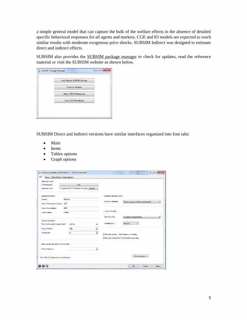
SUBSIM also provides the SUBSIM package manager to check for updates, read the reference
material or visit the SUBSIM website as shown below.
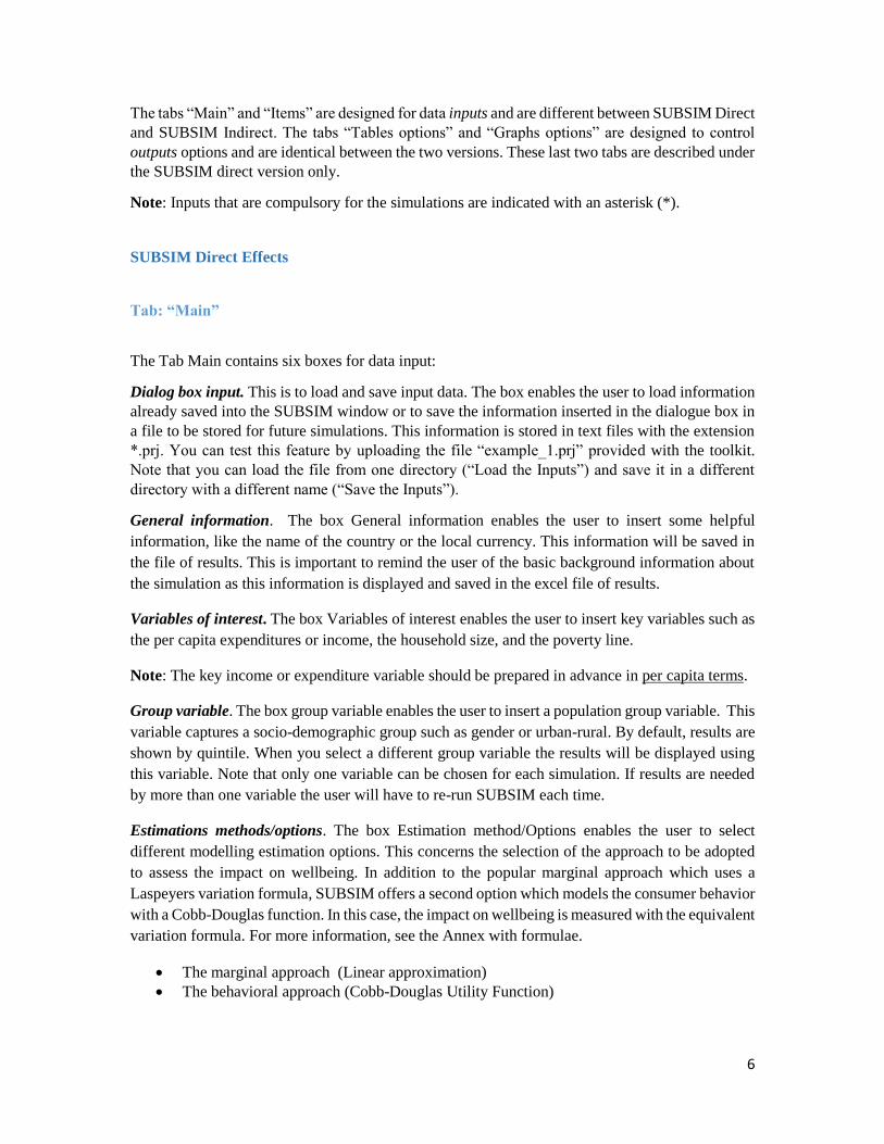
SUBSIM Direct and Indirect versions have similar interfaces organized into four tabs:
Main
Items
Tables options
Graph options
6
The tabs “Main” and “Items” are designed for data inputs and are different between SUBSIM Direct
and SUBSIM Indirect. The tabs “Tables options” and “Graphs options” are designed to control
outputs options and are identical between the two versions. These last two tabs are described under
the SUBSIM direct version only.
Note: Inputs that are compulsory for the simulations are indicated with an asterisk (*).
SUBSIM Direct Effects
Tab: “Main”
The Tab Main contains six boxes for data input:
Dialog box input. This is to load and save input data. The box enables the user to load information
already saved into the SUBSIM window or to save the information inserted in the dialogue box in
a file to be stored for future simulations. This information is stored in text files with the extension
*.prj. You can test this feature by uploading the file “example_1.prj” provided with the toolkit.
Note that you can load the file from one directory (“Load the Inputs”) and save it in a different
directory with a different name (“Save the Inputs”).
General information. The box General information enables the user to insert some helpful
information, like the name of the country or the local currency. This information will be saved in
the file of results. This is important to remind the user of the basic background information about
the simulation as this information is displayed and saved in the excel file of results.
Variables of interest. The box Variables of interest enables the user to insert key variables such as
the per capita expenditures or income, the household size, and the poverty line.
Note: The key income or expenditure variable should be prepared in advance in per capita terms.
Group variable. The box group variable enables the user to insert a population group variable. This
variable captures a socio-demographic group such as gender or urban-rural. By default, results are
shown by quintile. When you select a different group variable the results will be displayed using
this variable. Note that only one variable can be chosen for each simulation. If results are needed
by more than one variable the user will have to re-run SUBSIM each time.
Estimations methods/options. The box Estimation method/Options enables the user to select
different modelling estimation options. This concerns the selection of the approach to be adopted
to assess the impact on wellbeing. In addition to the popular marginal approach which uses a
Laspeyers variation formula, SUBSIM offers a second option which models the consumer behavior
with a Cobb-Douglas function. In this case, the impact on wellbeing is measured with the equivalent
variation formula. For more information, see the Annex with formulae.
The marginal approach (Linear approximation)
The behavioral approach (Cobb-Douglas Utility Function)
7
Lumpsum transfer. The box “Lump-sum transfer” enables the user to indicate information on cash
transfers. In some cases, government may want to compensate the population affected by subsidies
reforms with cash transfers. This box allow users to choose whether this transfer should be allocated
to individuals or households (Type of transfer: Individual or household) or whether the transfer
should be universal or targeted to particular population groups (Targeting form: Universal or
population group). There is no need to indicate the amount of transfers. Results are reported in
graphs and the user can select a range of values of transfers (the min and the max, see graphs
options) and see results for all values included in the range specified.
The tab “Main” also offers the options of leaving behind the welfare variables of the impact on
well-being and the quantities variables before and after simulations for each product. These
quantities are estimated by SUBSIM using information on expenditure and unit prices. If these
boxes are ticked, users will find these variables in the data set after SUBSIM has finished running.
Note: If users want to target a specific population group, the corresponding indicator should be
prepared in advance if not already part of the variables set. For example, poor=1 and non-poor=0
if the poor only should be targeted. If the group variable is not specified, SUBSIM will produce the
graphs on transfers with universal transfers.
NB: Survey settings. Remember to set the survey settings before you launch SUBSIM including
sampling weights and sampling design information. This can be done with the command “svyset”
in Stata or you can use the button “Survey Settings…” located in the bottom right-hand corner of
the SUBSIM “Main” tab. For more information on survey settings, see the Stata manual.
Tab “Items”
The Tab “Items” is conceived to insert information about the goods concerned by the simulation
including initial prices, final prices and unit subsidies.
Initialize information with: The information on products can be initialized manually by inserting
the information for each item (option “parameters values”) or by selecting variables already created
and available in the data set (option: “variables”). The “example.dta” contains these special
variables. Users would normally input data manually using the parameters values option unless one
needs to analyze more than ten items, which is the limit in the dialogue box. This is usually not
recommended because more than ten items make graphs very messy. If you have more than ten
items, divide them in separate simulations, for example dividing food and energy subsidies.
Number of items. This is to select the number of items to consider. The maximum number allowed
is ten.
Option “Parameter values”: With this option the user can input the information for each item
manually including name, quantity, per capita expenditure variables, type of price schedule, initial
price, unit subsidy, final price and elasticity.
8
Short names: This is the name of the variable as it should appear in the output files. This is
imputed manually.
Q. Unit: This is to insert the unit quantity (kg, liters, etc.). This information will be
displayed in the results tables.
Varnames: These variables are selected from the data set and indicate the variables that
contain information on expenditure per capita of the item considered.
Price schedules. Users have an option to choose linear and non-linear prices. This refers to
whether the price is equal for all quantities consumed by households or changes according
to quantities. This is the case, for example, of electricity or a product with a quota system
where households are entitled to subsidized prices only up to a certain quantity (quota).
Initial Prices. This is the pre-reform price, usually the subsidized price as found at the time
of simulations.
Subsidy: This is the unit subsidy. This information is usually provided by ministries or
specialized governmental agencies. Unit prices can also be estimated manually if the total
amount of subsidies on a product is known together with information on the quantity of
subsidized product consumed. Note that SUBSIM can also be used to simulate price
increases or decreases in the absence of subsidies. In this case, unit subsidies are set to zero.
Final prices: This is the simulated price. If one wants to remove subsidies completely, this
price will be simply the sum of the initial price and the unit subsidy. If one want to estimate
other price increases of reduction in subsidies this final price will be lower.
Elasticity. This is the own-price (quantity/price) elasticity. The user can insert any value
and this is used to estimate changes in quantities consumed and other impacts. See the
Annex for a discussion on how to specify the value of elasticity.
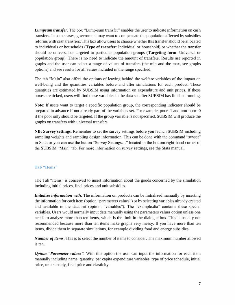
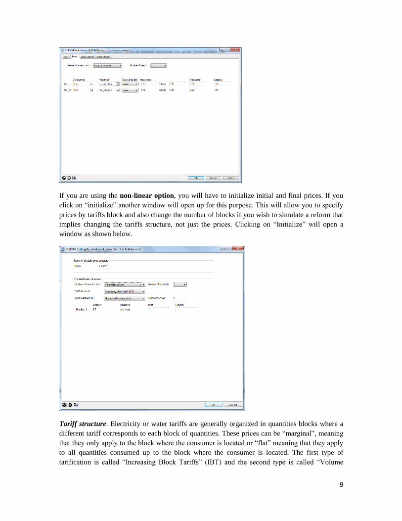
As an example, assume that the actual initial price is 0.1 monetary unit and the unit subsidy is 0.3.
In the absence of subsidies, the price of flour would be 0.4. We can simulate however any increase
in price such as an increase in prices of 0.1 which leads to a final price of 0.2. In this case, our
inputs will be 0.1 for the initial price, 0.3 for the unit subsidy and 0.2 for the final price. For rice,
we can input, as an example, 0.14 for the initial price, 0.4 for the unit subsidy and 0.24 for the final
price (see figure below).
9
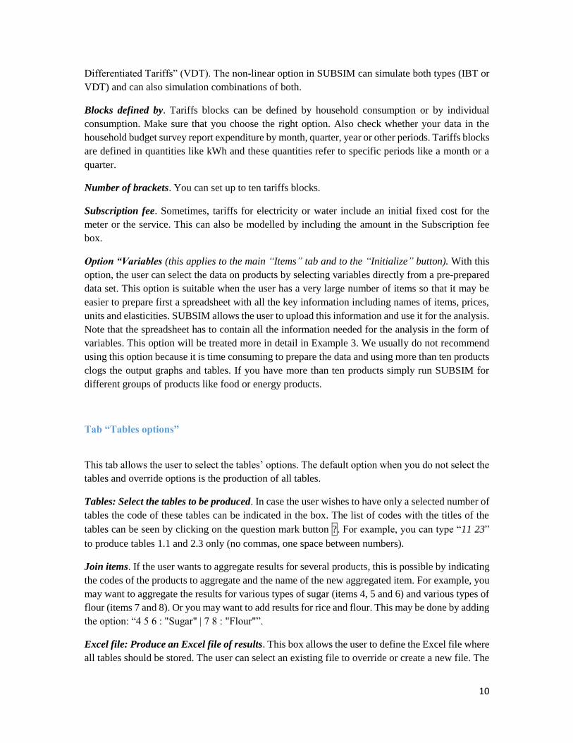
If you are using the non-linear option, you will have to initialize initial and final prices. If you
click on “initialize” another window will open up for this purpose. This will allow you to specify
prices by tariffs block and also change the number of blocks if you wish to simulate a reform that
implies changing the tariffs structure, not just the prices. Clicking on “Initialize” will open a
window as shown below.
Tariff structure. Electricity or water tariffs are generally organized in quantities blocks where a
different tariff corresponds to each block of quantities. These prices can be “marginal”, meaning
that they only apply to the block where the consumer is located or “flat” meaning that they apply
to all quantities consumed up to the block where the consumer is located. The first type of
tarification is called “Increasing Block Tariffs” (IBT) and the second type is called “Volume
10
Differentiated Tariffs” (VDT). The non-linear option in SUBSIM can simulate both types (IBT or
VDT) and can also simulation combinations of both.
Blocks defined by. Tariffs blocks can be defined by household consumption or by individual
consumption. Make sure that you choose the right option. Also check whether your data in the
household budget survey report expenditure by month, quarter, year or other periods. Tariffs blocks
are defined in quantities like kWh and these quantities refer to specific periods like a month or a
quarter.
Number of brackets. You can set up to ten tariffs blocks.
Subscription fee. Sometimes, tariffs for electricity or water include an initial fixed cost for the
meter or the service. This can also be modelled by including the amount in the Subscription fee
box.
Option “Variables (this applies to the main “Items” tab and to the “Initialize” button). With this
option, the user can select the data on products by selecting variables directly from a pre-prepared
data set. This option is suitable when the user has a very large number of items so that it may be
easier to prepare first a spreadsheet with all the key information including names of items, prices,
units and elasticities. SUBSIM allows the user to upload this information and use it for the analysis.
Note that the spreadsheet has to contain all the information needed for the analysis in the form of
variables. This option will be treated more in detail in Example 3. We usually do not recommend
using this option because it is time consuming to prepare the data and using more than ten products
clogs the output graphs and tables. If you have more than ten products simply run SUBSIM for
different groups of products like food or energy products.
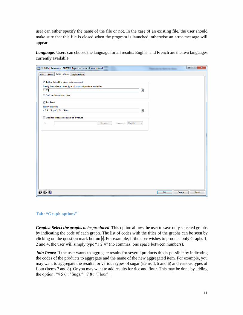
Tab “Tables options”
This tab allows the user to select the tables’ options. The default option when you do not select the
tables and override options is the production of all tables.
Tables: Select the tables to be produced. In case the user wishes to have only a selected number of
tables the code of these tables can be indicated in the box. The list of codes with the titles of the
tables can be seen by clicking on the question mark button ?. For example, you can type “11 23”
to produce tables 1.1 and 2.3 only (no commas, one space between numbers).
Join items. If the user wants to aggregate results for several products, this is possible by indicating
the codes of the products to aggregate and the name of the new aggregated item. For example, you
may want to aggregate the results for various types of sugar (items 4, 5 and 6) and various types of
flour (items 7 and 8). Or you may want to add results for rice and flour. This may be done by adding
the option: “4 5 6 : "Sugar" | 7 8 : "Flour"”.
Excel file: Produce an Excel file of results. This box allows the user to define the Excel file where
all tables should be stored. The user can select an existing file to override or create a new file. The
11
user can either specify the name of the file or not. In the case of an existing file, the user should
make sure that this file is closed when the program is launched, otherwise an error message will
appear.
Language: Users can choose the language for all results. English and French are the two languages
currently available.
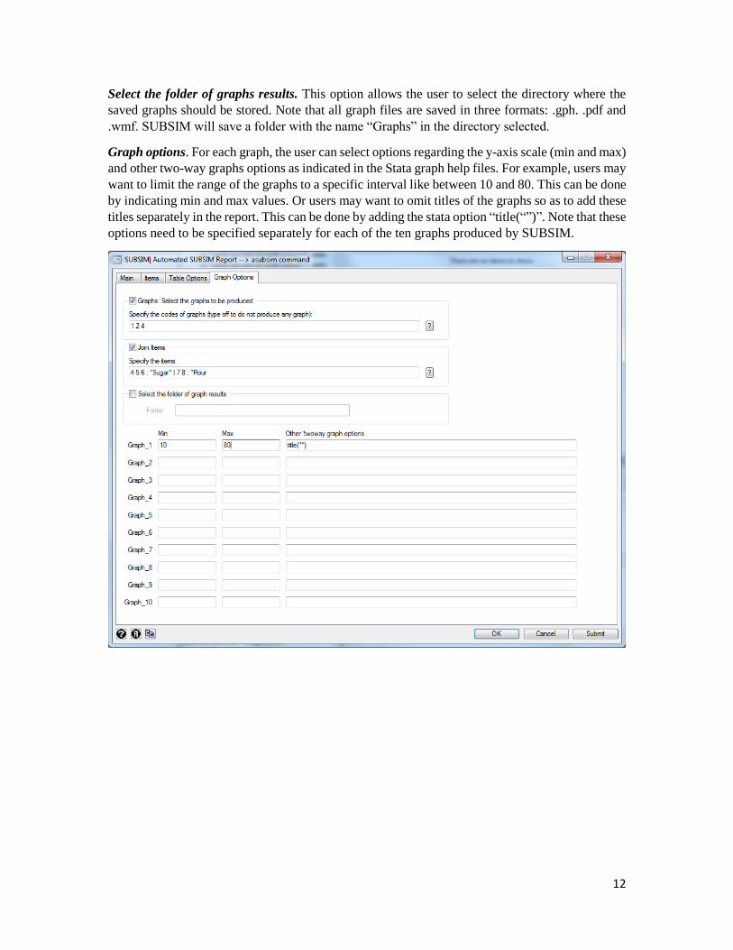
Tab: “Graph options”
Graphs: Select the graphs to be produced. This option allows the user to save only selected graphs
by indicating the code of each graph. The list of codes with the titles of the graphs can be seen by
clicking on the question mark button ?. For example, if the user wishes to produce only Graphs 1,
2 and 4, the user will simply type “1 2 4” (no commas, one space between numbers).
Join Items: If the user wants to aggregate results for several products this is possible by indicating
the codes of the products to aggregate and the name of the new aggregated item. For example, you
may want to aggregate the results for various types of sugar (items 4, 5 and 6) and various types of
flour (items 7 and 8). Or you may want to add results for rice and flour. This may be done by adding
the option: “4 5 6 : "Sugar" | 7 8 : "Flour"”.
12
Select the folder of graphs results. This option allows the user to select the directory where the
saved graphs should be stored. Note that all graph files are saved in three formats: .gph. .pdf and
.wmf. SUBSIM will save a folder with the name “Graphs” in the directory selected.
Graph options. For each graph, the user can select options regarding the y-axis scale (min and max)
and other two-way graphs options as indicated in the Stata graph help files. For example, users may
want to limit the range of the graphs to a specific interval like between 10 and 80. This can be done
by indicating min and max values. Or users may want to omit titles of the graphs so as to add these
titles separately in the report. This can be done by adding the stata option “title(“”)”. Note that these
options need to be specified separately for each of the ten graphs produced by SUBSIM.
13
Examples
For the examples, you will need to download first the data set and the examples files from the
following website:
http://www.subsim.org/examples/example_dir.rar
Example 1: Linear subsidies
The following examples are based on the data set “example.dta” provided with the toolkit. It is
recommended to run the example with the data provided before testing SUBSIM with other data.
This will ensure that SUBSIM has been correctly installed.
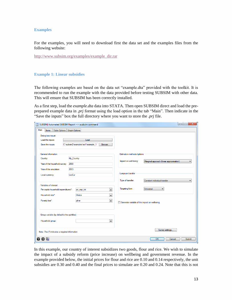
As a first step, load the example.dta data into STATA. Then open SUBSIM direct and load the pre-
prepared example data in .prj format using the load option in the tab “Main”. Then indicate in the
“Save the inputs” box the full directory where you want to store the .prj file.
In this example, our country of interest subsidizes two goods, flour and rice. We wish to simulate
the impact of a subsidy reform (price increase) on wellbeing and government revenue. In the
example provided below, the initial prices for flour and rice are 0.10 and 0.14 respectively, the unit
subsidies are 0.30 and 0.40 and the final prices to simulate are 0.20 and 0.24. Note that this is not
14
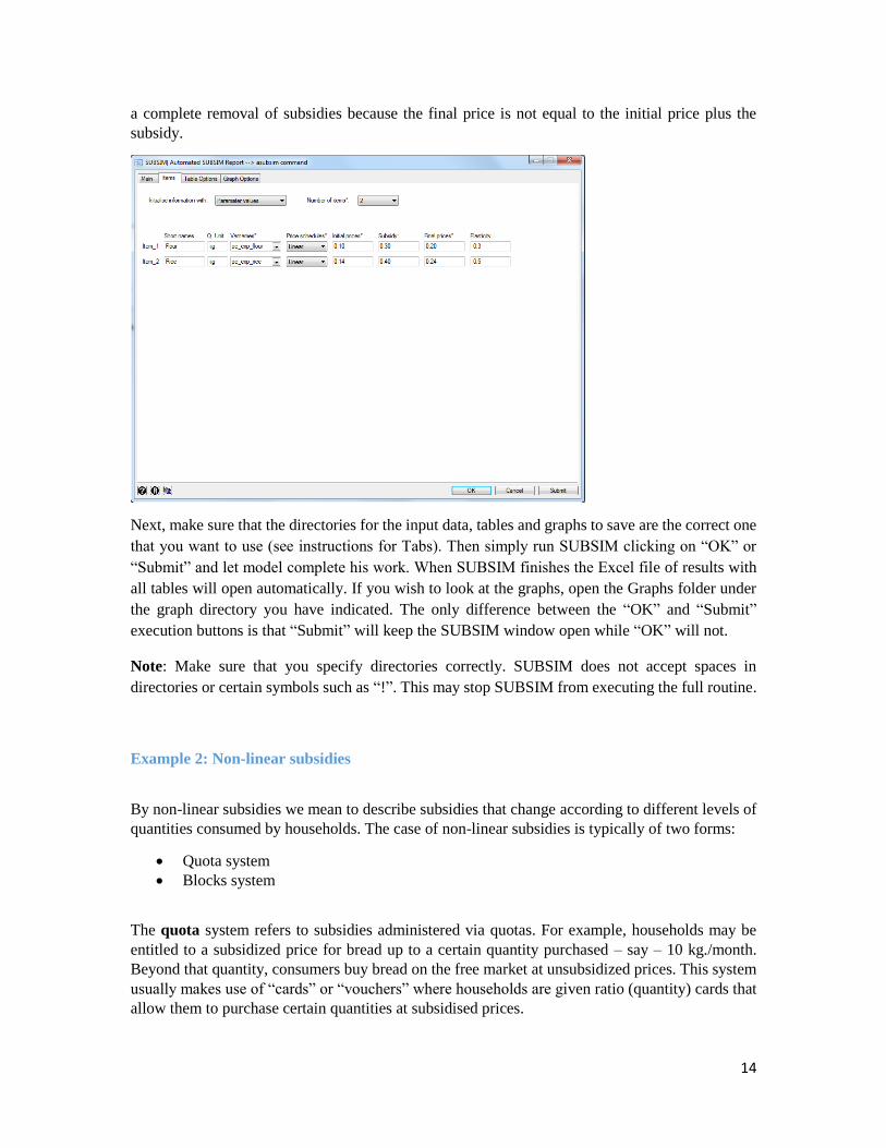
a complete removal of subsidies because the final price is not equal to the initial price plus the
subsidy.
Next, make sure that the directories for the input data, tables and graphs to save are the correct one
that you want to use (see instructions for Tabs). Then simply run SUBSIM clicking on “OK” or
“Submit” and let model complete his work. When SUBSIM finishes the Excel file of results with
all tables will open automatically. If you wish to look at the graphs, open the Graphs folder under
the graph directory you have indicated. The only difference between the “OK” and “Submit”
execution buttons is that “Submit” will keep the SUBSIM window open while “OK” will not.
Note: Make sure that you specify directories correctly. SUBSIM does not accept spaces in
directories or certain symbols such as “!”. This may stop SUBSIM from executing the full routine.
Example 2: Non-linear subsidies
By non-linear subsidies we mean to describe subsidies that change according to different levels of
quantities consumed by households. The case of non-linear subsidies is typically of two forms:
Quota system
Blocks system
The quota system refers to subsidies administered via quotas. For example, households may be
entitled to a subsidized price for bread up to a certain quantity purchased – say – 10 kg./month.
Beyond that quantity, consumers buy bread on the free market at unsubsidized prices. This system
usually makes use of “cards” or “vouchers” where households are given ratio (quantity) cards that
allow them to purchase certain quantities at subsidised prices.
15
The blocks system refers to subsidies that change following a “block” structure with different
prices applying to different blocks of quantities consumed. This is typically the case of electricity
or water subsidies where the electricity or water prices are set by the regulator at different prices
for each quantity block. For example, a price for a consumption of 0-150 kWh/month, a higher
price for a consumption of 151-300 kWh/month and so on. In this case, the number of blocks can
be small or large depending on the choice of the regulator.
From an economic and modelling perspective the quota and blocks systems are equivalent. In fact,
the quota system can be considered as a block system with a two blocks’ structure. Therefore, in
what follows, we will limit our example to the quota system but the same explanations apply to the
blocks system.
Suppose now that subsidies are administered through a quota system where all individuals are
entitled to fixed quantities at subsidised prices. For example, imagine that the annual per capita
quota for flour is 36 kg. Assume also that the non-subsidized market price is equal to 0.4. This
implies that the price of flour is non-linear; it changes with different quantities consumed.
Consumers pay a subsidized price up to 36 kg per person and the unsubsidized price for any
additional quantity purchased. The following table summarizes the flour non-linear schedule price.
Block by Subsidy Price
0-36 kg individual 0.3 0.1
36 kg and more --- 0.0 0.4
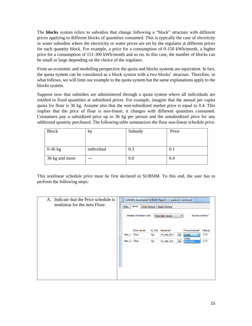
This nonlinear schedule price must be first declared in SUBSIM. To this end, the user has to
perform the following steps:
A. Indicate that the Price schedule is
nonlinear for the item Flour.
16
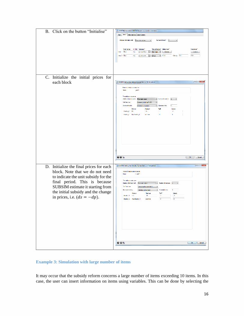
B. Click on the button “Initialise”
C. Initialize the initial prices for
each block
D. Initialize the final prices for each
block. Note that we do not need
to indicate the unit subsidy for the
final period. This is because
SUBSIM estimate it starting from
the initial subsidy and the change
in prices, i.e. (𝑑𝑠 = −𝑑𝑝).
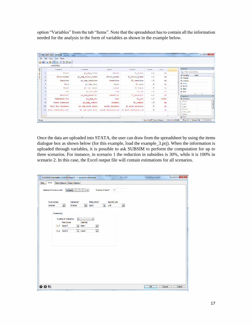
Example 3: Simulation with large number of items
It may occur that the subsidy reform concerns a large number of items exceeding 10 items. In this
case, the user can insert information on items using variables. This can be done by selecting the
17
option “Variables” from the tab “Items”. Note that the spreadsheet has to contain all the information
needed for the analysis in the form of variables as shown in the example below.
Once the data are uploaded into STATA, the user can draw from the spreadsheet by using the items
dialogue box as shown below (for this example, load the example_3.prj). When the information is
uploaded through variables, it is possible to ask SUBSIM to perform the computation for up to
three scenarios. For instance, in scenario 1 the reduction in subsidies is 30%, while it is 100% in
scenario 2. In this case, the Excel output file will contain estimations for all scenarios.
18
When you have tested the three examples, you are ready to use SUBSIM direct with your own data.
Don’t forget to prepare you data file in advance following the indications provided.
SUBSIM Indirect Effects
The main objective of SUBSIM indirect is to estimate the direct and indirect effects of a price
change on household wellbeing combining a Household Budget Survey (HBS) and Input-Output
(I/O) tables for a particular country. Note that SUBSIM indirect focuses only on the goods that are
concerned by the exogenous price shocks. Thus, this version is more appropriate to assess the
indirect effect rather than the full direct effect of the subsidy reform. Direct effects are better
estimated with SUBSIM direct.
Data and methodology
SUBSIM Indirect requires at least one Household Budget Survey (HBS) and an Input-Output (I/O)
matrix (file). The I/O matrix required is the output matrix expressed in local currency. It is
important that the I/O data and the HBS data are expressed in the same currency, in nominal terms
and for the same year. In general, it will be difficult to obtain I/O tables and HBS data for the same
year. This implies that either the HBS, or the I/O data or both will need to be adjusted for prices to
make data in nominal terms comparable and for the same reference year. This work has to be done
by users before using SUBSIM Indirect.
Note that the last line of the I/O matrix should be the total value added also called total primary
input (total output-total intermediate inputs).
In order for SUBSIM to match HBS data with I/O data, users have to prepare HBS consumption
aggregates that mimic the I/O sectors in advance. Since HBS products are much more numerous
than I/O sectors, one would want to group sets of HBS products corresponding to I/O sectors so
that SUBSIM can do a one to one matching between HBS aggregates of products and I/O sectors.
In some cases, one HBS product may span across several I/O sectors. SUBSIM can also handle this
last case. The user will simply indicate in the dialogue box multiple I/O sectors corresponding to a
single aggregate of HBS products (or one product).
This is how SUBSIM indirect operates. Suppose that we want to study the direct and indirect
welfare effects of a price increase of gasoline. Since I/O tables are organized by sector and it is
very rare for researchers to have access to I/O tables by individual product, the study of indirect
effects can only be done by sector and group of products and not by individual product. In our
example, we have one sector called “petroleum products” which includes gasoline as well as other
products. We can shock this sector with a price increase and study the direct and indirect effects on
final consumers. If users have detailed information on the sector structure and want to study the
effect of a price change of only one product, it is possible to make the price shock proportionate to
the importance of the product within the sector. For example, if gasoline accounts for only 20% of
the petroleum sector and we wish to increase only the price of gasoline by 10%, one can shock the
petroleum sector by 2% (10% of 20%). This is a user’s choice and does not make any difference to
how SUBSIM operates.
19
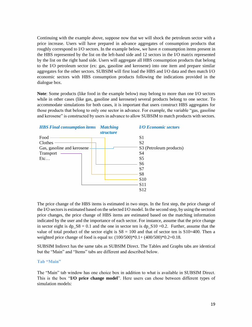
Continuing with the example above, suppose now that we will shock the petroleum sector with a
price increase. Users will have prepared in advance aggregates of consumption products that
roughly correspond to I/O sectors. In the example below, we have n consumption items present in
the HBS represented by the list on the left-hand side and 12 sectors in the I/O matrix represented
by the list on the right hand side. Users will aggregate all HBS consumption products that belong
to the I/O petroleum sector (ex: gas, gasoline and kerosene) into one item and prepare similar
aggregates for the other sectors. SUBSIM will first load the HBS and I/O data and then match I/O
economic sectors with HBS consumption products following the indications provided in the
dialogue box.
Note: Some products (like food in the example below) may belong to more than one I/O sectors
while in other cases (like gas, gasoline and kerosene) several products belong to one sector. To
accommodate simulations for both cases, it is important that users construct HBS aggregates for
those products that belong to only one sector in advance. For example, the variable “gas, gasoline
and kerosene” is constructed by users in advance to allow SUBSIM to match products with sectors.
HBS Final consumption items Matching
structure
I/O Economic sectors
Food S1
Clothes S2
Gas, gasoline and kerosene
S3 (Petroleum products)
Transport
S4
Etc… S5
S6
S7
S8
S10
S11
S12
The price change of the HBS items is estimated in two steps. In the first step, the price change of
the I/O sectors is estimated based on the selected I/O model. In the second step, by using the sectoral
price changes, the price change of HBS items are estimated based on the matching information
indicated by the user and the importance of each sector. For instance, assume that the price change
in sector eight is dp_S8 = 0.1 and the one in sector ten is dp_S10 =0.2. Further, assume that the
value of total product of the sector eight is S8 = 100 and that of sector ten is S10=400. Then a
weighted price change of food is equal to: (100/500)*0.1+ (400/500)*0.2=0.18.
SUBSIM Indirect has the same tabs as SUBSIM Direct. The Tables and Graphs tabs are identical
but the “Main” and “Items” tabs are different and described below.
Tab “Main”
The “Main” tab window has one choice box in addition to what is available in SUBSIM Direct.
This is the box “I/O price change model”. Here users can chose between different types of
simulation models:
20
M1: Cost-push prices. The main assumption here is that producers “push” the increase in
prices onto consumers via the increase in prices of market products. SUBSIM Indirect
offers two sets of options (exogenous/endogenous model and short-term/long-term).
Endogenous and exogenous model: This refers to the sector that is shocked. With
the endogenous option, we enable for the price adjustment of the shocked sector
after the shock period. With the exogenous option, we assume that the price of the
shocked sector does not change after the introduction of the price shock. Of course,
the selection of the appropriate model will depend on the country context. For
instance, if the country is a net importer of the shocked good, and we assume that
is economy cannot really influence the world price, it may be appropriate to select
the exogenous model.
Short-term or Long-term: This refers to the time horizon of the price effects
measured in terms of successive rounds of price adjustments. The short-term
option considers only the first round effects. The long-term option considers
infinite rounds.
M2: Marginal profit-push prices. The main assumption here is that markets are competitive
and reach full price adjustments and producers maintain their marginal profits in the long-
term. For the formulae corresponding to this choice see Annex with formulae.
Tab “Items”
The new ‘Items” tab window has two panels: 1) Items info and 2) Price shock and I/O matrix info.
Remember that items indicated with an asterisk (*) are mandatory.
Items info: This panel is designed to input data from the HBS file. Here you have two options. If
you have up to ten items, you can input the information related to these items directly from the
window (option “Parameters value”). If you have more than 10 items, you need to prepare these
items in advance in the HBS file (option “Variables”). In this case, the HBS file has to be prepared
and loaded in advance and must contain the variables that indicate the item names, the
corresponding variables names and elasticity if required by the user. Look in the example provided
to see how the key variables are constructed.
Short names. This is the space to indicate the names of items as displayed in results.
Varnames. The user should also indicate the variable that contains the items already matched with
the I/O economic sectors. This variable will contain the group of HBS products that roughly
correspond to I/O sectors.
Elasticity. This is the own-price elasticity to use for the simulations. See appendix for more
information on how to set elasticities.
21
Matching I/O sectors: This is where the I/O sectors matching the HBS variable indicated in
“Varnames” are indicated. As already mentioned, since HBS products are more numerous than I/O
sectors, one would want to group sets of HBS products under individual I/O sectors so that
SUBSIM can do a one to one matching between HBS aggregates of products and I/O sectors.
However, in some cases, one group of HBS product may span across several I/O sectors. SUBSIM
can also handle this last case. The user will simply indicate multiple I/O sectors corresponding to
a single aggregate of HBS products in the box “Matching I/O sectors”. Otherwise, this box will
contain only one matching sector. Matching sectors are indicated with numbers as found in the I/O
data file.
Note: The file directory of the input file should not contain any space and the last line of the I/O
matrix data file must contain the added values as shown in the example below for a hypothetical
I/O matrix with four sectors.
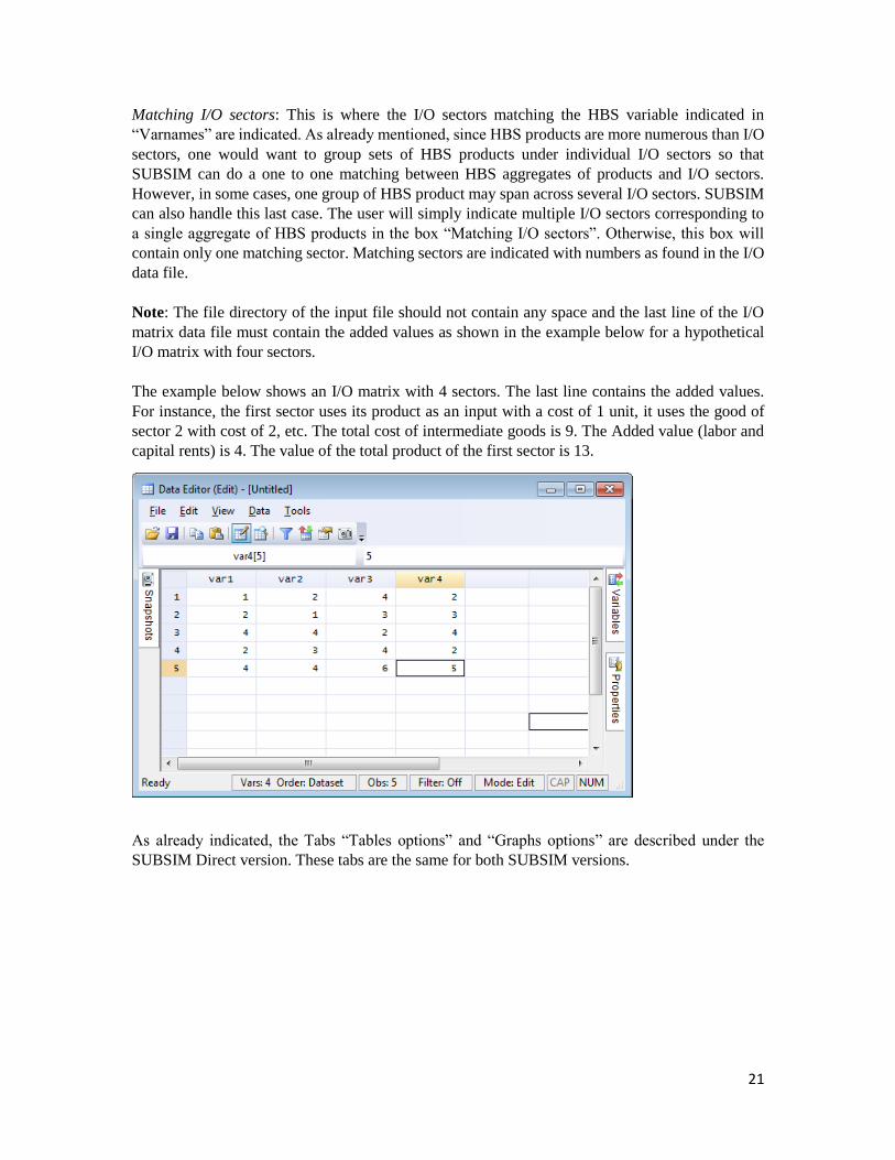
The example below shows an I/O matrix with 4 sectors. The last line contains the added values.
For instance, the first sector uses its product as an input with a cost of 1 unit, it uses the good of
sector 2 with cost of 2, etc. The total cost of intermediate goods is 9. The Added value (labor and
capital rents) is 4. The value of the total product of the first sector is 13.
As already indicated, the Tabs “Tables options” and “Graphs options” are described under the
SUBSIM Direct version. These tabs are the same for both SUBSIM versions.
22
Example
As an example, load the zipped file below from the internet and unzip the file in your working
directory:
http://www.subsim.org/examples/example_ind.rar
The zipped file contains data files (.dta) and pre-loaded input file (.pri). The three data files include
a HBS file (“example_ind_eff.dta”), an I/O data file (“iomv.dta”) and a file containing the sectors
legenda of the I/O file (“sec_info”). The pri files contain information on examples that can be
directly loaded into windows.
Note: The .pri file extension is used in place of the .prj file extension so as to distinguish between
SUBSIM Direct and SUBSIM Indirect input files.
As you can see, the I/O file (“iomv.dta”) contains 50 lines and 49 columns (49 sectors plus one line
for the value added). The HBS file (“example_ind_eff.dta”) contains the per capita consumption of
nine main items:
1. food
2. clothes
3. energy (dir_eff)
4. transport
5. electricity
6. travel_tourism
7. telecomunication
8. habits
9. education
The HBS file also contains the variables with the items full names (“itnames”) and variable names
(“nitems”). These are the variables that you would use if you have more than ten items and cannot
create these same variables from SUBSIM windows. The file also contains other information used
by SUBSIM such as total consumption per capita, household size or the poverty line.
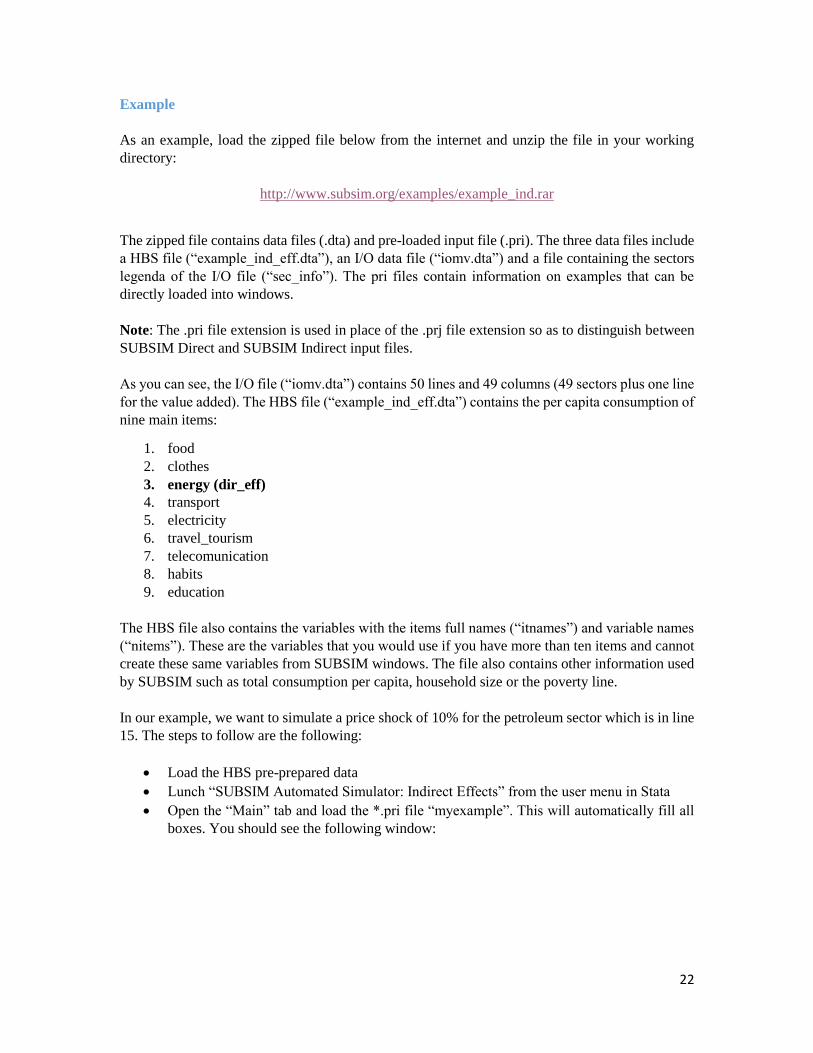
In our example, we want to simulate a price shock of 10% for the petroleum sector which is in line
15. The steps to follow are the following:
Load the HBS pre-prepared data
Lunch “SUBSIM Automated Simulator: Indirect Effects” from the user menu in Stata
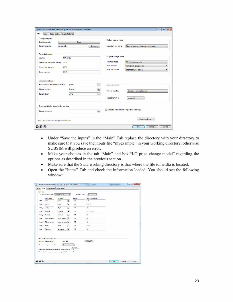
Open the “Main” tab and load the *.pri file “myexample”. This will automatically fill all
boxes. You should see the following window:
23
Under “Save the inputs” in the “Main” Tab replace the directory with your directory to
make sure that you save the inputs file “myexample” in your working directory, otherwise
SUBSIM will produce an error.
Make your choices in the tab “Main” and box “I/O price change model” regarding the
options as described in the previous section.
Make sure that the Stata working directory is that where the file iomv.dta is located.
Open the “Items” Tab and check the information loaded. You should see the following
window:
24
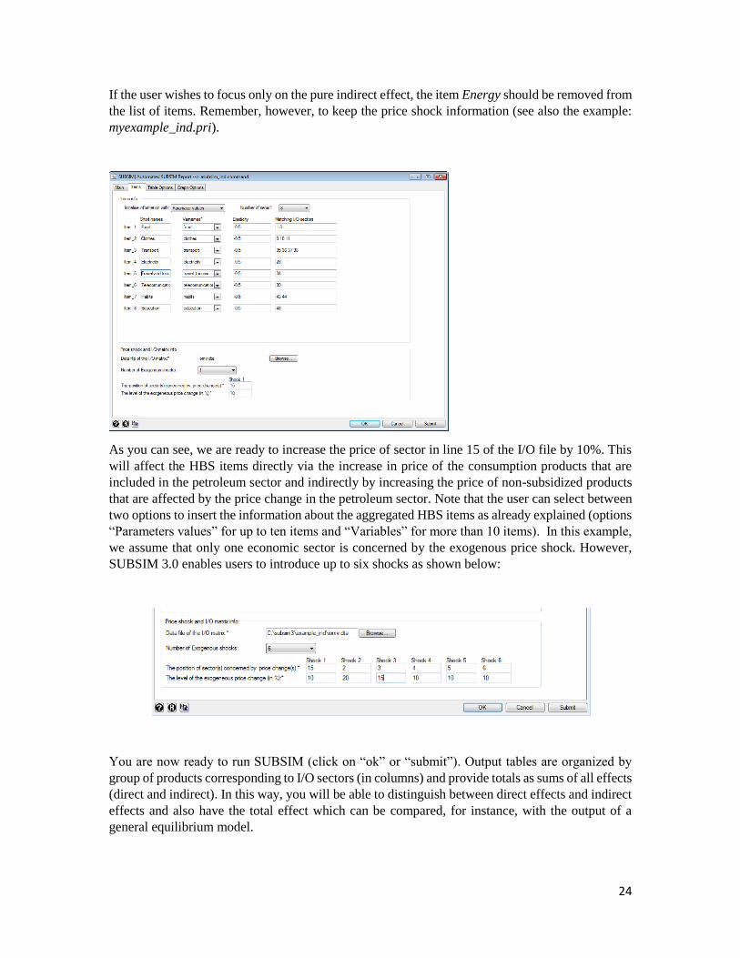
If the user wishes to focus only on the pure indirect effect, the item Energy should be removed from
the list of items. Remember, however, to keep the price shock information (see also the example:
myexample_ind.pri).
As you can see, we are ready to increase the price of sector in line 15 of the I/O file by 10%. This
will affect the HBS items directly via the increase in price of the consumption products that are
included in the petroleum sector and indirectly by increasing the price of non-subsidized products
that are affected by the price change in the petroleum sector. Note that the user can select between
two options to insert the information about the aggregated HBS items as already explained (options
“Parameters values” for up to ten items and “Variables” for more than 10 items). In this example,
we assume that only one economic sector is concerned by the exogenous price shock. However,
SUBSIM 3.0 enables users to introduce up to six shocks as shown below:
You are now ready to run SUBSIM (click on “ok” or “submit”). Output tables are organized by
group of products corresponding to I/O sectors (in columns) and provide totals as sums of all effects
(direct and indirect). In this way, you will be able to distinguish between direct effects and indirect
effects and also have the total effect which can be compared, for instance, with the output of a
general equilibrium model.
25
Note: To avoid typical mistakes, make sure that: 1) the HBS data have been loaded in advance; 2)
the specified directory for the I/O data is correct and without spaces; 3) the specified directory
under “Save the inputs” in the “Main” Tab is your directory and not the one pre-loaded.
When you run SUBSIM the program follows the following sequence of actions:
1) Matches products with sectors using information provided in the tab “Items”
2) Picks the simulation algorithm selected with choices in the tab “Main”
3) Produces the matrix of coefficients “A” (see appendix)
4) Introduces shocks to the system following the choice made in the tab “Items”
5) Calculates the impact on all sectors
6) Derives the impact on group of products as selected in the tab “Items”
7) Produces tables of results in one excel file as indicated in the tab “Tables”
8) Produces a folder with Figures as indicated in the tab “Figures:
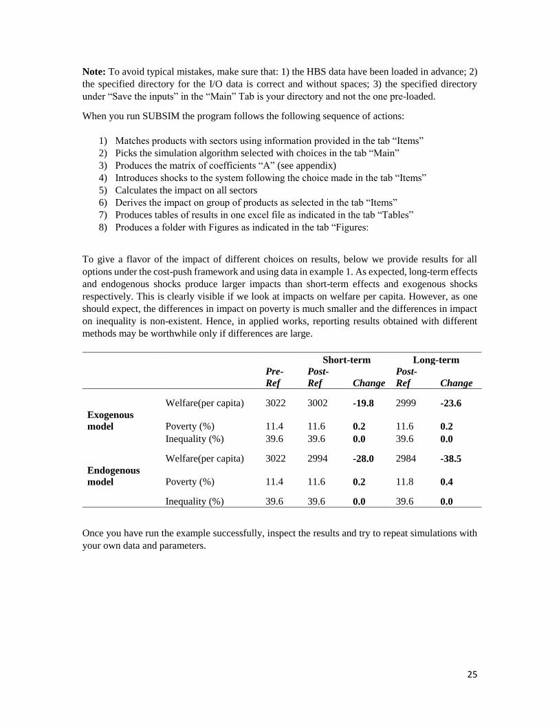
To give a flavor of the impact of different choices on results, below we provide results for all
options under the cost-push framework and using data in example 1. As expected, long-term effects
and endogenous shocks produce larger impacts than short-term effects and exogenous shocks
respectively. This is clearly visible if we look at impacts on welfare per capita. However, as one
should expect, the differences in impact on poverty is much smaller and the differences in impact
on inequality is non-existent. Hence, in applied works, reporting results obtained with different
methods may be worthwhile only if differences are large.
Short-term Long-term
Pre-
Ref
Post-
Ref Change
Post-
Ref Change
Welfare(per capita) 3022 3002 -19.8 2999 -23.6
Exogenous
model Poverty (%) 11.4 11.6 0.2 11.6 0.2
Inequality (%) 39.6 39.6 0.0 39.6 0.0
Welfare(per capita) 3022 2994 -28.0 2984 -38.5
Endogenous
model Poverty (%) 11.4 11.6 0.2 11.8 0.4
Inequality (%) 39.6 39.6 0.0 39.6 0.0
Once you have run the example successfully, inspect the results and try to repeat simulations with
your own data and parameters.
26
Launch SUBSIM
When SUBSIM is launched, it will display all results in the Stata output window. The user can stop
the command at any stage of execution by using the Stata “Break” button. If the user has selected
to save the table results in an Excel file, this file is automatically opened once the computation
ends. The excel file produced contains one table per sheet and all tables produced by the program.
All graphs produced by the program are instead saved in a folder with the name “Graphs”, and in
three formats (pdf, gph and wmf).
The complete set of tables and graphs can then be used to prepare a report on the distribution of
subsidies, on the impact of subsidies reforms on household welfare and the government revenues
and on the impact of compensatory cash transfers on poverty and the government budget. If the
user is familiar with SUBSIM and all input information is available, SUBSIM will produce results
in a few minutes and a full report can be prepared in a few days. Moreover, all the data input are
saved by users in a file with the .prj or .pri files extensions. This allows for an easy update or
reproduction of results at any time.
Comparing SUBSIM Direct and SUBSIM Indirect effects
SUBSIM Direct and SUBSIM Indirect can be used independently depending on data availability
and simulation needs. In some cases, users may want to use both versions and compare results. This
is not straightforward and this section explains how to compare and interpret results for direct and
indirect effects when both models are used. Recall that SUBSIM Direct produces only direct first-
round effects while SUBSIM Indirect produces direct and indirect effects combined for first and
higher rounds.
As a first rule, SUBSIM direct will always be more accurate than SUBSIM Indirect to estimate
direct effects. That is because results are displayed by individual product and the price shocks can
be applied to individual products rather than economic sectors. Hence, SUBSIM Direct exploits at
best available HBS information and results in SUBSIM Direct should be used as the reference
results for direct effects in empirical analyses.
It is also possible to separate direct and indirect effects using SUBSIM Indirect. This is done by
opting for the cost-push model with the exogenous option. The exogenous option is enough to
ensure that the introduced price shock in sector X does not affect the same sector in subsequent
rounds. Hence, for single products simulations and with the cost-push exogenous option, results of
SUBSIM Indirect under the shocked sector are the same as SUBSIM Direct results under the
shocked product (see example below).
Note that comparing SUBSIM Direct and SUBSIM Direct is possible if one shocks one product at
a time. More complex simulations with multiple price shocks will make comparisons between the
two SUBSIM versions more complex because of cross-products and cross-sectors effects. Hence,
a good strategy is to analyze one product at a time and see how important direct effects are in
relation to indirect effects. This is a good strategy also because different products have typically
very different shares of direct and indirect effects. For example, diesel, which is largely used for
commercial transport but not by households, has very large indirect effects but moderate direct
effects. Vice-versa, LPG, which is largely consumed by households but not used very much as a
27
production input, will have large direct effects but small indirect effects. An analysis that combines
simultaneous shocks on diesel and LPG will miss on these important differences.
As an example, we compare simulations for a price increase in diesel with SUBSIM Direct with a
corresponding price increase in the Diesel sector (Petroleum) with SUBSIM Indirect. The case-
study is Morocco and the increase in price of diesel is 11.35%. This is the price increase used in
SUBSIM Direct. For SUBSIM Indirect we need to multiply this price increase for the share of
diesel in the petroleum sector. Thus, the price shock to apply in SUBSIM Indirect is
[11.35*(57.23/100)] = 6.5%.
It is important to note here that the share of diesel in the sector is not derived from I/O data but
from HBS data. In this particular case, we have only two products that correspond to the oil-refining
sector in I/O tables and these two products are grouped under the HBS sector “Petroleum”. Diesel
represents 57.23% of the petroleum sector according to HBS data and this is the share (weight) to
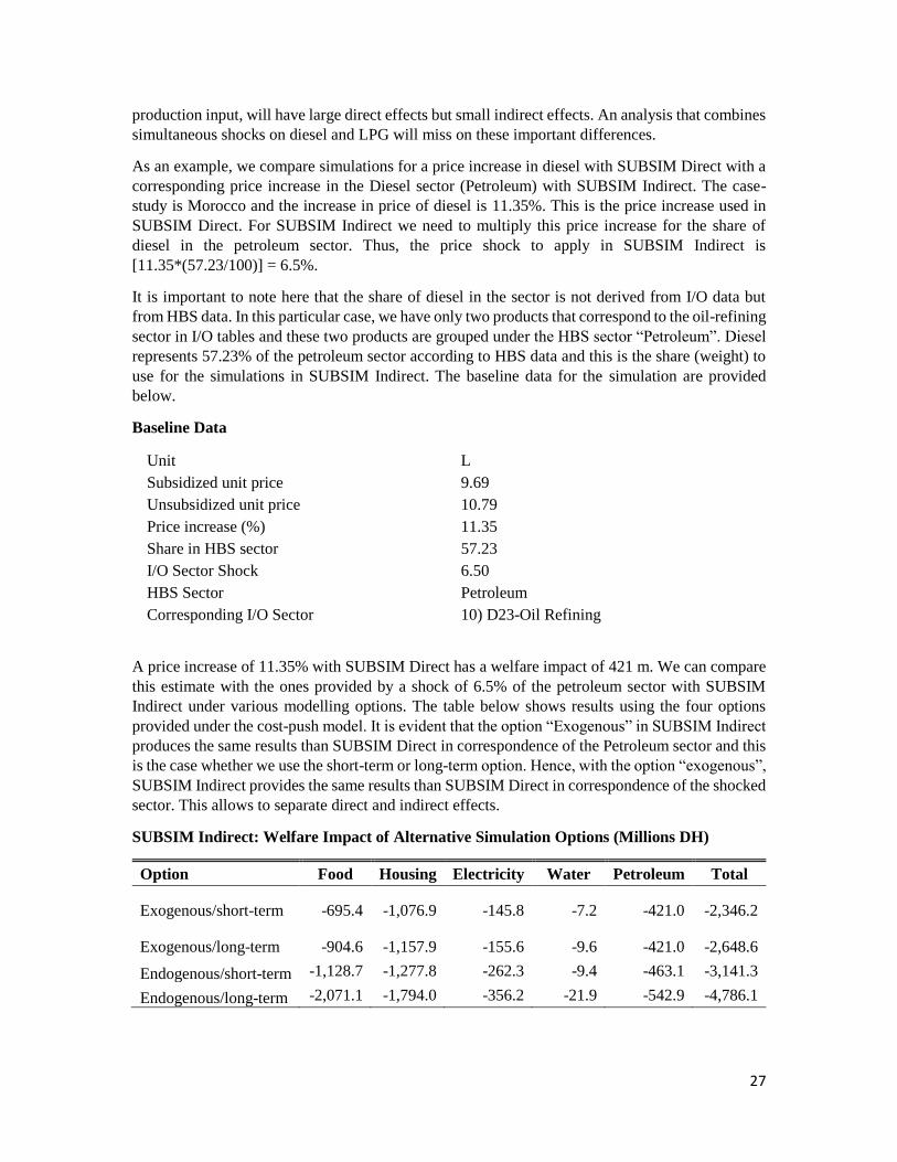
use for the simulations in SUBSIM Indirect. The baseline data for the simulation are provided
below.
Baseline Data
Unit L
Subsidized unit price 9.69
Unsubsidized unit price 10.79
Price increase (%) 11.35
Share in HBS sector 57.23
I/O Sector Shock 6.50
HBS Sector Petroleum
Corresponding I/O Sector 10) D23-Oil Refining
A price increase of 11.35% with SUBSIM Direct has a welfare impact of 421 m. We can compare
this estimate with the ones provided by a shock of 6.5% of the petroleum sector with SUBSIM
Indirect under various modelling options. The table below shows results using the four options
provided under the cost-push model. It is evident that the option “Exogenous” in SUBSIM Indirect
produces the same results than SUBSIM Direct in correspondence of the Petroleum sector and this
is the case whether we use the short-term or long-term option. Hence, with the option “exogenous”,
SUBSIM Indirect provides the same results than SUBSIM Direct in correspondence of the shocked
sector. This allows to separate direct and indirect effects.
SUBSIM Indirect: Welfare Impact of Alternative Simulation Options (Millions DH)
Option Food Housing Electricity Water Petroleum Total
Exogenous/short-term -695.4 -1,076.9 -145.8 -7.2 -421.0 -2,346.2
Exogenous/long-term -904.6 -1,157.9 -155.6 -9.6 -421.0 -2,648.6
Endogenous/short-term -1,128.7 -1,277.8 -262.3 -9.4 -463.1 -3,141.3
Endogenous/long-term -2,071.1 -1,794.0 -356.2 -21.9 -542.9 -4,786.1

28
Annex 1 – SUBSIM Basic Formulae
This annex provides a brief introduction to the basic formulae used by SUBSIM. The first version
of SUBSIM (SUBSIM 1.0) was accompanied by a full paper: Araar, A. and Verme, P. (2012)
Reforming Subsidies: A Toolkit for Policy Simulations, World Bank Policy Research Working
Paper No. 6148. The paper includes a general section on subsidies simulations, a section on the
economic theory behind SUBSIM and the SUBSIM 1.0 users’ guide. The sections below integrate
and update the theoretical part of the paper for SUBSIM 2.0.
Changes in welfare
Let e=monetary expenditure; p=price and q=quantities with the superscripts ‘ representing the post-
reform values, the subscript 1 representing the subsidized product and the subscript 2 representing
the bundle of all other consumed products. It is well-known that the total expenditures (e) can be
used as a money metric measurement of wellbeing. The change in welfare, due to an increase in
price, depends on the change in consumed quantities. Mainly, we have:
e = p1q1 + p2q2
e′ = p1′ q1
′ + p2q2′
When prices are normalised at consumer equilibrium, the last consumed units of each of the two
goods will generate the same level of utility. With the assumption of marginal or moderate change
in prices, the consumer can select any combination of quantities (q1′ , q2
′ ), but the decrease in
wellbeing is practically the same. Based on this assumption, an easy way to assess the change in
wellbeing is the case where the change in quantities concerns only the first good.
∆𝑤 = ∆𝑞1 = −𝑞1 dp1
Since prices are normalised, we can also write:
∆𝑤=−𝑒1 dp1
where dp represents the relative price change (∆𝑝1/𝑝1). This is the most popular method to estimate
changes in welfare subject to changes in prices and is the same approach proposed by Coady et al.
(2006) among others.
Note that this formula applies with any behavioral response on the part of households including
changes in quantities consumed of the subsidized products or substitution of the subsidized product
with consumption of other products. This means that the use of elasticities in SUBSIM does not
affect the estimation of the impact of subsidies reforms on household welfare. Households can
reorganize consumption as they wish but the impact on total household welfare will not change.
In the case of multiple pricing of the product considered (for example electricity with different
tariffs for different quantities consumed) the formula for the changes in household welfare is as
follows:
29
∆𝑤ℎ = − ∑ 𝑒1,ℎ,𝑏𝑑𝑝1,𝑏
𝐵
𝑏=1
where b represents the blocks and h households. The sum across households represents the total
change in welfare.
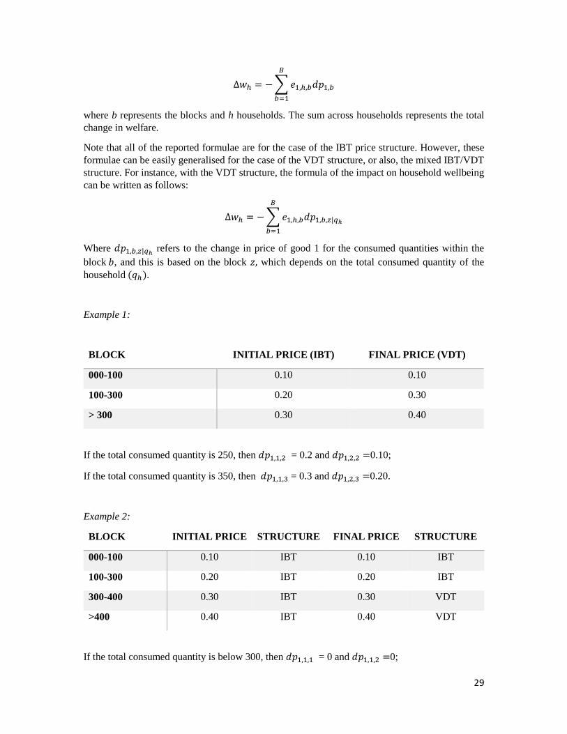
Note that all of the reported formulae are for the case of the IBT price structure. However, these
formulae can be easily generalised for the case of the VDT structure, or also, the mixed IBT/VDT
structure. For instance, with the VDT structure, the formula of the impact on household wellbeing
can be written as follows:
∆𝑤ℎ = − ∑ 𝑒1,ℎ,𝑏𝑑𝑝1,𝑏,𝑧|𝑞ℎ
𝐵
𝑏=1
Where 𝑑𝑝1,𝑏,𝑧|𝑞ℎ refers to the change in price of good 1 for the consumed quantities within the
block 𝑏, and this is based on the block 𝑧, which depends on the total consumed quantity of the
household (𝑞ℎ).
Example 1:
BLOCK INITIAL PRICE (IBT) FINAL PRICE (VDT)
000-100 0.10 0.10
100-300 0.20 0.30
> 300 0.30 0.40
If the total consumed quantity is 250, then 𝑑𝑝1,1,2 = 0.2 and 𝑑𝑝1,2,2 =0.10;
If the total consumed quantity is 350, then 𝑑𝑝1,1,3 = 0.3 and 𝑑𝑝1,2,3 =0.20.
Example 2:
BLOCK INITIAL PRICE STRUCTURE FINAL PRICE STRUCTURE
000-100 0.10 IBT 0.10 IBT
100-300 0.20 IBT 0.20 IBT
300-400 0.30 IBT 0.30 VDT
>400 0.40 IBT 0.40 VDT
If the total consumed quantity is below 300, then 𝑑𝑝1,1,1 = 0 and 𝑑𝑝1,1,2 =0;
30
If the total consumed quantity is 350, then 𝑑𝑝1,1,3 = 0.2 and 𝑑𝑝1,2,3 =0.10.
If the total consumed quantity is 450, then 𝑑𝑝1,1,4 = 0.3, 𝑑𝑝1,2,4 =0.2 and 𝑑𝑝1,3,4 =0.1.
SUBSIM also allows to model household behavior using a Cobb-Douglas function. In the case of
multiple pricing of the product considered the formula is as follows:
∆𝑤 = 𝑒1,ℎ (1
∏ 𝜑𝑚,ℎ𝛼𝑚,ℎ 𝑀
𝑚=1
− 1)
Where 𝜑𝑚,ℎ is the average weighted post reform price (the post reform price in the linear case) of
household ℎ for the good 𝑚 and 𝛼𝑚,ℎ is the expenditure share of household ℎ for the good 𝑚.
The marginal approach is the most common method and it is usually accurate for small or moderate
price increases. For very large price increases, the marginal approach tends to overestimate the
welfare impact and it is recommended to use the Cobb-Douglas approach.
Changes in quantities
Estimates of changes in quantities in the consumption of the subsidized product are useful to have
an idea on the impact of the subsidy reforms on quantities consumed and, by consequence, on
production of subsidized goods. They are also essential to estimate the impact of reforms on
government revenues given that the government reduces expenditure on subsidies when households
reduce consumption of subsidized products. Estimates on changes in quantities, in turn, require
knowledge of the demand function and the price-quantity elasticity of the subsidized product.
SUBSIM assumes a linear demand function and allows for imputing elasticities. The basic formula
for the estimation of changes in quantities of the subsidized product is
∆𝑞1 = 𝑞1𝑑𝑝1𝜀1
where the own price elasticity 𝜀1 is typically negative and between 0 and -1. Note that we are
assuming that all households behave equally so that the total impact on quantities is just the sum of
the changes in quantities consumed across all households.
Elasticity
The formula for the estimation of changes in quantities consumed uses the own-price
uncompensated elasticity. One of the main difficulties in subsidies simulations is to specify the
value of this elasticity correctly. There are at least three major difficulties.
The first difficulty is that it is very hard to estimate elasticities when products are subsidized. When
prices are subsidized and especially when only one price is applied nationally and on all quantities,
it is not possible to estimate the own-price elasticity cross-section with a model based on household
data (there is no price variation). Sometime, the subsidized price changes over time and one may
have available several household consumption surveys that cover the period when price changes
occurred. However, this is rare and it is very difficult to isolate the impact of the price change in
31
the subsidized product from other effects on expenditure over time. Therefore, subsidies analysts
can rarely estimate elasticities for the country of interest.
The second difficulty relates to the use of known elasticities from the literature and other countries.
Sometimes, it is possible to derive elasticity parameters from the specific literature on products.
For example, the own-price elasticity for gasoline is quite well known and has been estimated
widely worldwide and the user could simply use estimations made for similar countries to the
country of interest. However, known elasticities are typically estimated at free market prices and
they are point elasticities that apply to prices that are not subsidized. The point elasticities at
subsidized prices may be very different and cannot be assumed to be the same. Therefore, it is very
difficult for subsidies analysts to simply “borrow” elasticities from elsewhere.
The third difficulty is that the formula presented in the previous section is designed for small
changes in prices (marginal changes) and does not function well for large price changes. When the
product between changes in prices and elasticity (𝑑𝑝1𝜀1) is greater than 1, the post-reform quantity
can become negative using this formula. Unlike other simulations of price changes, changes in
subsidized prices can be very large, especially when governments want to remove subsidies
altogether. In these cases, it is not unusual to have price increases of several folds so that 𝑑𝑝1 can
be very large. Therefore, subsidies analysts cannot simply use standard parameters for elasticities
like -0.3 or -0.5 but have to consider more specifically the relation between subsidized and
unsubsidized prices before specifying elasticities.
To overcome these problems, SUBSIM has three main solutions. The first solution is that, by
design, SUBSIM does not allow quantities to become negative (−𝑄0) because the post-reform
quantity has a lower bound of zero. However, one should be aware that when results on quantities
in the Excel output file show zero values, it is most likely that the specified elasticities are too large.
Subsidized products are usually essential consumption items and it is unlikely that households stop
consuming these products altogether if the price increases. It is more likely that our specification
of elasticity is incorrect.
The second solution is to use the value of elasticity at unsubsidized prices from another country
and derive from this elasticity the correct elasticity to use for the subsidized price. When the
subsidized price is several folds lower than the unsubsidized price, this means that the subsidized
price is extremely low. But if this price is extremely low and quantity is initially high, we should
expect the own-price elasticity to be very low. If prices increase a little around the subsidized price,
consumers will tend to reduce quantities by very small amounts. On the contrary, if the subsidized
price is very close to the unsubsidized price then it is more likely that increases in prices will lead
to large decreases in quantities and that the elasticity will be large. Hence, either the elasticity 𝜀1 is
large or the relative change in price 𝑑𝑝1 is large but they should not be both large at the same time.
As a rule of thumb, if the new price is three times the current price and the known elasticity at
unsubsidized prices is (say) -0.3, then the elasticity to use in the formula may be around a third of
that value, say 0.1.
With the assumption of a straight linear demand function, it is also possible to calculate precisely
the initial elasticity (the elasticity at the subsidized price) using the final elasticity (the elasticity at
the unsubsidized price). The formula is as follows:
32
𝜀1 =
(1
(1 −𝜀1
′ (𝑝1′ − 𝑝1)𝑝1
′ )− 1)
(𝑝1′ − 𝑝1)
𝑝1
The third (and perhaps the most sensible) solution is to run SUBSIM with different assumptions
about the elasticity and compare results. In this case, it is useful to use zero as a lower bound and
the expected value of elasticity at the unsubsidized price as an upper value. This is what we would
recommend especially when price increases are very large.
Changes in government revenues
Having discussed elasticities and changes in quantities, we can now estimate changes in
government revenues. We may face two cases, one where we know the unit subsidy and one where
we don’t know the unit subsidy in advance. If we know the unit subsidy, the formula is as follows:
∆𝑟 = ∑ ek,hdpk (1 − 𝜀𝑘( sk − dpk))
H
h=1
where sk is the unit subsidy for product k.
In the case of large price changes and in order to constrain the maximum decrease in quantity to
that of the initial quantity, the formula becomes:
∆r = ∑ ek,hdpk + max(εkek,hdpk ; −ek,h)
H
h=1
(dpk − sk)
If we don’t know the unit subsidy in advance, we can then approximate the change in government
revenues with the change in producers’ profits as follows:
∆𝑟 = ∑ −𝑒𝑘,ℎ𝑑𝑝𝑘 (1 + 𝜀𝑘 (1 + 𝑑𝑝𝑘))
𝐻
ℎ=1
SUBSIM will use one or the other formula depending on whether users specify unit subsidies or
not in the Tab “Items”.
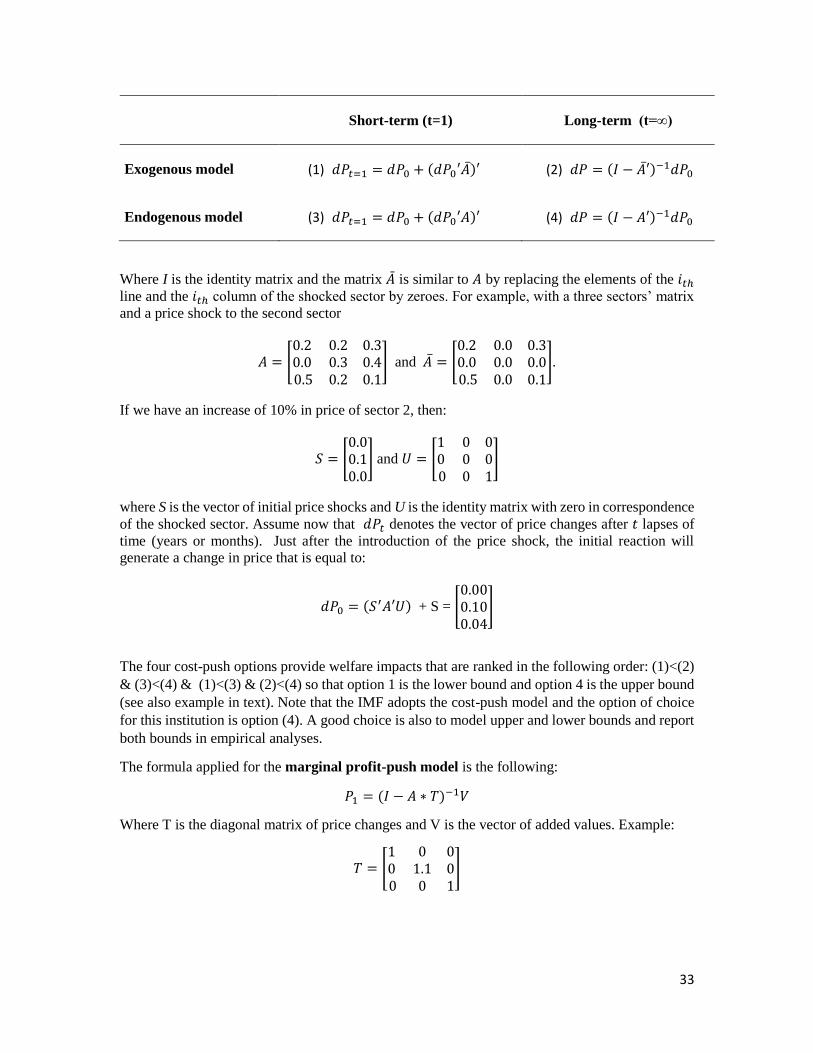
Formulae for input-output simulations
SUBSIM Indirect provides various options for the simulation of indirect effects with input-output
tables. The two sets of choices for the cost-push model will select one of four options for the
estimation of direct and indirect effects. The formulae of the four options are listed in the table
below:
33
Short-term (t=1) Long-term (t=∞)
Exogenous model (1) 𝑑𝑃𝑡=1 = 𝑑𝑃0 + (𝑑𝑃0′�̅�)′ (2) 𝑑𝑃 = (𝐼 − �̅�′)−1𝑑𝑃0
Endogenous model (3) 𝑑𝑃𝑡=1 = 𝑑𝑃0 + (𝑑𝑃0′𝐴)′ (4) 𝑑𝑃 = (𝐼 − 𝐴′)−1𝑑𝑃0
Where I is the identity matrix and the matrix �̄� is similar to 𝐴 by replacing the elements of the 𝑖𝑡ℎ
line and the 𝑖𝑡ℎ column of the shocked sector by zeroes. For example, with a three sectors’ matrix
and a price shock to the second sector
𝐴 = [0.2 0.2 0.30.0 0.3 0.40.5 0.2 0.1
] and �̅� = [0.2 0.0 0.30.0 0.0 0.00.5 0.0 0.1
].
If we have an increase of 10% in price of sector 2, then:
𝑆 = [0.00.10.0
] and 𝑈 = [1 0 00 0 00 0 1
]
where S is the vector of initial price shocks and U is the identity matrix with zero in correspondence
of the shocked sector. Assume now that 𝑑𝑃𝑡 denotes the vector of price changes after 𝑡 lapses of
time (years or months). Just after the introduction of the price shock, the initial reaction will
generate a change in price that is equal to:
𝑑𝑃0 = (𝑆′𝐴′𝑈) + S = [0.000.100.04
]
The four cost-push options provide welfare impacts that are ranked in the following order: (1)<(2)
& (3)<(4) & (1)<(3) & (2)<(4) so that option 1 is the lower bound and option 4 is the upper bound
(see also example in text). Note that the IMF adopts the cost-push model and the option of choice
for this institution is option (4). A good choice is also to model upper and lower bounds and report
both bounds in empirical analyses.
The formula applied for the marginal profit-push model is the following:
𝑃1 = (𝐼 − 𝐴 ∗ 𝑇)−1𝑉
Where T is the diagonal matrix of price changes and V is the vector of added values. Example:
𝑇 = [1 0 00 1.1 00 0 1
]