SUBMITTED TO IEEE TRANSACTIONS ON WIRELESS · PDF fileMassive MIMO, or a large-scale antenna array system, is the deployment of a very large number of antenna elements at base stations

SUBMITTED TO IEEE TRANSACTIONS ON WIRELESS COMMUNICATIONS 1

On Reusing Pilots Among Interfering Cells inMassive MIMO

Jy-yong Sohn, Sung Whan Yoon, Student Member, IEEE, and Jaekyun Moon, Fellow, IEEE

Abstract—Pilot contamination, caused by the reuse of pilotsamong interfering cells, remains as a significant obstacle that lim-its the performance of massive multi-input multi-output antennasystems. To handle this problem, less aggressive reuse of pilotsinvolving allocation of additional pilots for interfering users isclosely examined in this paper. Hierarchical pilot reuse methodsare proposed, which effectively mitigate pilot contamination andincrease the net throughput of the system. Among the suggestedhierarchical pilot reuse schemes, the optimal way of assigningpilots to different users is obtained in a closed-form solutionwhich maximizes the net sum-rate in a given coherence time.Simulation results confirm that when the ratio of the channelcoherence time to the number of users in each cell is sufficientlylarge, less aggressive reuse of pilots yields significant performanceadvantage relative to the case where all cells reuse the same pilotset.

Index Terms—Massive MIMO, Multi-user MIMO, Multi-cellMIMO, Pilot contamination, Pilot assignment, Pilot reuse, Inter-ference, Large-scale antenna system, Channel estimation

I. INTRODUCTION

SUPPORTING the stringent requirements of the next gen-eration wireless communication systems is an ongoing

challenge, especially given the foreseeable scenarios wheremassively-deployed devices rely on applications with high-throughput (e.g. virtual/augmented reality) and/or low latency(e.g. autonomous vehicles). This unavoidable trend gives riseto discussions on the technology for next generation com-munications, collectively referred to as 5G. Regarding theengineering requirements of high data rate, low latency, andhigh energy efficiency, attractive 5G technologies in [2]–[5]include massive multi-input multi-output (MIMO) [6]–[8],ultra-densification [9]–[11] and millimeter wave (mm-Wave)communications among other things.

Massive MIMO, or a large-scale antenna array system, isthe deployment of a very large number of antenna elementsat base stations (BSs), possibly orders of magnitude largerthan the number of user terminals (UTs) served by each BS[12], [13]. Assuming M , the number of BS antennas, increaseswithout bound, the asymptotic analysis on capacity and otherfundamental aspects of massive MIMO were presented in [13],[14]. The work of [13], in particular, has demonstrated thatin time-division duplex (TDD) operation with uplink trainingfor attaining channel-state-information (CSI), the effects ofuncorrelated noise and fast fading disappear as M grows to

The authors are with the School of Electrical Engineering, Korea AdvancedInstitute of Science and Technology, Daejeon, 305-701, Republic of Korea (e-mail: [email protected], [email protected], [email protected]). Thispaper was presented in part at IEEE ICC 2015 Workshop on 5G & Beyond[1].

infinity, with no cooperation necessary among BSs. Accordingto this “channel-hardening” behavior, [13] concluded thatin a single-cell setting where UTs have orthogonal pilots,capacity increases linearly with K, the number of UTs, asM/K increases even without channel knowledge. However,in multi-cell setting, the channel estimation errors due to pilotcontamination prevent the linear growth of the sum rate withK. Pilot contamination is caused by the reuse of pilots amongdifferent cells and persists even as the number of BS antennasincreases without limit; it remains as a fundamental issue inmassive MIMO [15].

Various researchers have since investigated systematic meth-ods to mitigate the pilot contamination effect [1], [16]–[28].Some researchers exploited the angle-of-arrival (AoA) infor-mation to combat pilot contamination. A coordinated pilotassignment strategy was suggested based on AoA informationwhich can eliminate channel estimation error as the numberof BS antennas increases without bound [16], [17]. However,favorable AoA distributions are not always guaranteed in realscenarios. In addition, significant challenges remain on actu-ally getting AoA information and managing network overloadfor cooperation.

Another approaches have focused on precoding to reducethe pilot contamination effect. The work of [18] suggesteda distributed single-cell linear minimum mean-square-error(MMSE) precoding, which exploits pilot sequence informationto minimize the error caused by inter-cell and intra-cellinterference. The proposed precoding scheme has improvedperformance compared to the conventional single-cell zero-forcing (ZF) precoder, but cannot completely eliminate pilotcontamination. In [19], outer multi-cellular precoding underthe assumption of cooperating BSs was introduced for miti-gating the pilot contamination effect. The suggested methodis based on adjusting the precoding vector according to thecontaminated channel estimate via coordinated information.Backhaul network overload for realizing cooperation remainsas an issue in realizing this precoding scheme.

The impact of pilot transmission protocol is considered in[20]–[23]. Shifting of pilot frames corresponding to neigh-boring cells was proposed, which mitigated pilot contam-ination [20]. Appropriate power allocation to increase thesignal-to-interference ratio (SIR) in shifted pilot frame wasalso suggested [21]. Even though the shifted pilot framemethod avoided correlation between identical pilot sequences,it caused the correlation between pilot sequence and datasequence in the training phase. Central control is also requiredto achieve precise timing among shifted pilot frames, whichneeds additional overload. Another pilot transmission protocol

arX

iv:1

710.

0281

1v1

[cs

.IT

] 8

Oct

201

7


to eliminate pilot contamination was proposed in [22] basedon imposing a silent phase for each cell over successivetime slots during the training period. A linear combinationof observations taken over the successive training phasesallow simple elimination of inter-cell interferences while fullyreusing pilots across cells, but the method does not offer anyadvantage in terms of reducing total training time overheadcompare to the straightforward employment of LK orthogonalpilot symbols over all LK users across entire cells.

Pilot assignment strategies are also considered as an al-ternative to mitigate pilot contamination and to increase netthroughput [23]–[25], [29]. According to the strategy sug-gested in [23], the cell is divided into the center area andthe edge area; the users in the center employ the same pilotresource non-cooperatively, while cooperative resource allo-cation is applied to those in the edge. This strategy mitigatessevere pilot contamination for edge users, but still requirescooperation among BSs. A greedy algorithm (called smartpilot assignment) is suggested in [24], which assigns pilot withless inter-cell interference to the user with low channel quality.This approach improved the minimum signal-to-interference-plus-noise ratio (SINR) within each cell compared to randomassignment case, but requires cooperation between BSs inorder to exploit slow fading coefficients of entire cells. In[25], spectral efficiency (SE) was maximized with respectto pilot assignment, power allocation and the number ofantennas. Considering cell-free massive MIMO systems whereM antennas and K users are dispersed in a region, theauthors of [29] jointly optimized greedy pilot assignment andpower control to increase the achievable rate. However, thegreedy pilot assignment requires backhaul network, involvingcooperation between distributed antennas. According to thesepapers, optimal pilot assignment can increase SE comparedto random assignment, while finding the optimal solutionalso require BS cooperation. Moreover, [29] considers pilotassignment and power control for cell-free distributed antennasystems, whereas the present paper considers pilot allocationin multi-cellular systems with co-located antenna setting.

As seen above, most of the known effective solutions tocombat pilot contamination tend to rely heavily on cooperationamong BSs, leading to backhaul overload issues. Also, mostof the previous works assume full reuse of the same pilot setamong all cells and rarely discuss the potential associated withallowing more orthogonal pilots.

Some researchers investigated the effect of employing lessaggressive pilot reuse methods, but to limited extents [26]–[28]. A scenario of utilizing the number of pilots greaterthan K is considered in [26], which suggested a multi-cellMMSE detector exploiting all pilots in the system. It is shownthat the suggested multi-cell MMSE scheme can significantlyincrease spectral efficiency as the pilot reuse factor becomesless aggressive. An SE-maximizing massive MIMO system isconsidered in [27], which optimizes the number of scheduledusers K for given M and pilot reuse factor. The simulationresult shows that the optimal solution selects less aggressivepilot reuse for some practical scenarios. A pilot reuse factorof 3 (cell partitioning similar to frequency reuse of 3) isconsidered in [28], which is shown to be beneficial to mitigate

pilot contamination. However, only symmetric pilot reusepatterns (lattice structure) was considered in [28], and noclosed-form solution was found for the optimal pilot reusefactor; as such, the impact of partial pilot reuse was not madeclear.

In contrast, in [1] the present authors presented asystematically-constructed pilot reuse method to effectivelyreduce pilot contamination. Non-trivial hierarchical pilotreuse/assignment schemes are proposed, and a closed-formsolution to optimum pilot assignment is presented that max-imizes the net sum-rate. The present paper further analyzesthe pilot assignment strategy proposed in [1], providing formalproofs of the previously presented mathematical results and of-fering key insights into the physical significance of the optimalpilot assignment rule, along the way. Moreover, the presentpaper adds the analysis and finds optimal pilot assignmentassociated with a large but finite number of antennas, whereas[1] only provided an asymptotic result for BS with an infinitenumber of antennas. Physical insights on the optimal assign-ment for infinite M can be similarly observed for the finiteM case, while numerical results show that the net throughputbetween optimal assignment and conventional full pilot reusestill has a substantial gap, even in practical scenarios ofdeploying 100 − 1000 BS antennas. The present paper alsoinvestigates the ideal portion of pilot training allocated for theoptimal assignment strategy; this investigation points to theinteresting fact that in the optimal scheme a non-vanishingportion of the coherence interval is reserved for the pilots asNcoh/K grows.

Overall, this paper is about finding the optimal portionof pilot transmission as well as pilot reuse strategy whichmaximize the net sum-throughput, taking into account pilotcontamination due to interfering cells. This problem arisesin some meaningful practical scenarios but has not beenaddressed previously. Although the optimal portion of pilottraining was considered by several researchers [12], [30], [31],none of their works or any other previous related works to ourbest knowledge addressed the optimal pilot length and optimalpilot assignment in massive MIMO, where pilot contaminationlimits the performance and no constraint is imposed on thespecific pilot reuse method.

Compared to the ideal asymptotic analysis in [13], severalworks attempted to emphasize the practical aspects of applyingmassive MIMO in real-world systems. Considering BSs with afinite M , the achievable rate is obtained [32] when matched-filter (MF) or MMSE detection is used. Focusing on somepropagation environments where the channel hardening doesnot hold, [33] suggested a downlink blind channel estimationmethod. The behavior of massive MIMO systems with non-ideal hardware is observed in [34].

This paper is organized as follows. Section II gives anoverview of the system model for massive MIMO and the pilotcontamination effect. Section III discusses the assumptionsmade on cell geometry and basic partitioning steps neededto utilize longer pilots, and presents the mathematical analysisfor specifying the optimal pilot assignment strategy. The math-ematical results are first stated in [1], while the formal proofsand the key insights leading to physical interpretations of the


obtained results are provided in the present paper. In SectionIV, simulation results on the performance of the optimalpilot assignment are presented. Section V includes furthercomments on finite M analysis, optimal portion of pilots,cell partitioning in conventional frequency reuse, considerationof prioritized users and application in ultra-dense networks.Section VI finally draws conclusions.

II. PILOT CONTAMINATION EFFECT FOR MASSIVE MIMOMULTI-CELLULAR SYSTEM

A. System ModelWe assume that the network consists of L hexagonal cells

with K users per cell who are uniform-randomly located.Downlink CSIs are estimated at each BS by uplink pilottraining assuming channel reciprocity in TDD operation. Thispaper assumes the channel model in [27]; this model isappropriate for sufficiently large (M > 32) numbers of BSantennas, as tested in [35]. The singular value spread of themeasured channel is close to that of an i.i.d. Rayleigh channelmodel for a large number of antennas [35]. Therefore, weadopt this model. The complex propagation coefficient g of alink can be decomposed into a complex fast fading factor hand a slow fading factor β. Therefore, the channel between themth BS antenna of the jth cell and the kth user of the lth cellis modeled as gmjkl = hmjkl

√βjkl. The slow fading factor,

which accounts for the geometric attenuation and shadowfading, is modeled as βjkl = ( 1

rjkl)γ where rjkl is the distance

between the kth user in the lth cell and the base station in thejth cell. The parameter γ represents the signal decay exponent.Let Tcoh be the coherence time interval and Tdel be the channeldelay spread. It is convenient to express the coherence timeinterval as a dimensionless quantity, Ncoh = Tcoh/Tdel, vianormalization by channel delay spread.

B. Pilot Contamination EffectThe pilot contamination effect is the most serious issue that

arises in multi-cell TDD systems with very large BS antennaarrays. For uplink training, each BS collects pilot sequencessent by its users. Usually, orthogonal pilot sequences areassigned to users in a cell so that the channel estimate foreach user does not suffer from interferences from other usersin the same cell. However, the use of the same pilot sequencesfor users in other cells cause the channel estimates to becontaminated, and this effect, called pilot contamination, limitsthe achievable rate, even as M , the number of BS antennas,tends to infinity.

According to [13], under the assumption of a single userper cell, the achievable rate during uplink data transmissionfor the user in the jth cell contaminated by users with thesame pilot on other cells is given for a large M by

log2

(1 +

β2jj∑

l 6=j β2jl

)(1)

where βjl is the slow fading component of the channelbetween the jth BS and the interfering user in the lth cell.In the limit of large M , the achievable rate depends only onthe ratio of the signal to interference due to the pilot reuse.

(a) 3-way Partitioning

L

L/3 L/3 L/3

L/9 L/9 L/9 L/9 L/9 L/9 L/9 L/9 L/9

Depth = 0

Depth = 1

Depth = 2

(b) Hierarchical set partitinoing

Fig. 1: The Cell Partitioning Method

III. PILOT ASSIGNMENT STRATEGY

In this section, we provide analysis on how much timeshould be allocated for channel training given a coherencetime and how the pilot sequences should be assigned to userson multiple cells. We derive optimal pilot assignment strategy,which mitigates the pilot contamination effect and maximizestotal bits transmitted in a given Tcoh. Our analysis considersusing pilot sequences possibly longer than the number of usersin each cell, while orthogonality of the pilots within a cell isguaranteed.

A. Hexagonal-Lattice Based Cell Clustering and Pilot Assign-ment Rule

Consider L hexagonal cells. Imagine partitioning these cellsinto three equi-distance subsets maintaining the same latticestructure as depicted in Fig. 1a. This partitioning is identicalto the familiar partitioning of contiguous hexagonal cells forutilizing three frequency bands according to a frequency reusefactor of three.

It can easily be seen that each coset, having the samehexagonal lattice structure, can be further partitioned in thesimilar way. The partitioning can clearly be applied in asuccessive fashion, giving rise to the possibility of hierarchicalset partitioning of the entire cells. In the tree structure of Fig.1b, the root node (at depth 0) represents the original group of Lcontiguous hexagonal cells, and the three child nodes labeledL/3 correspond to the three colored-cosets of Fig. 1a. Also,applying a 3-way partitioning to a coset results in additionalthree child nodes with labels L/9. Note that a node at depthi corresponds to a subset of L3−i cells.

This cell clustering method is used to define pilot assign-ment rule in multi-cell system. Consider when each cell has asingle user (i.e., K = 1). Then, determining pilot sharing cellsspecifies the pilot assignment rule. In our approach, cells withsame color are defined to share same pilot, while cells withdifferent color have orthogonal pilots. In the correspondingtree structure, the number of leaves with different (non-white)colors represents the number of different orthogonal pilot sets


used. A leaf (end node) with a single cell would correspondto a depth of log3 L, but we do not allow such leaves in ouranalysis as this means there would be users with no pilotcontamination, thus driving the average per-cell throughput ofthe network to infinity as M grows. This particular situationwould not lend itself to a meaningful mathematical analysis.Thus, the maximum depth of a leaf in our tree is set tolog3 L− 1.

The pilot assignment rule can be generalized to the caseof having multiple users per cell (i.e., K > 1), by applyingthe procedure K times consecutively (K users in each cellobtain orthogonal pilots by K independent procedures). Notethat K procedures result in K partitioning trees, where eachtree represents pilot assigning rule of L users.

Note that the suggested pilot assignment strategy assumesuniform power allocation: every user has the same transmitpower for pilot. The suggested assignment focuses on reducingpilot contamination by placing pilot-sharing users in distantcells, and the optimal power allocation has not been consideredhere. According to the recent research [29] on pilot assignmentand power control within a cell, controlling transmit power forpilot among different users has a significant role in increasingspectral efficiency. This could be an interesting subject thatcould be pursued in conjunction with the suggested pilotassignment strategy, but we leave the pilot power control issueas a future research topic.

B. Pilot Assignment Vector

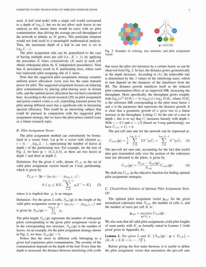
The pilot assignment method can conveniently be formu-lated in a vector form. Let p be a vector with element pi,i = 0, · · · , log3 L − 1, representing the number of leaves atdepth i of the partitioning tree. For example, for the tree ofFig. 2, we have p = (0, 2, 3, 0), as there are two leaves atdepth 1 and three at depth 2.

Definition: For the given L cells, denote PL,K as the set ofvalid pilot assignment vectors based on 3-way partitioning,which is given by

PL,K = p = (p0, p1, · · · , plog3 L−1) :

0 ≤ pi ≤ K3i,

log3 L−1∑i=0

pi3−i = K (2)

where it is implied that pi is an integer.

Definition: For the given L cells, Npil(p) is the length of thevalid pilot assignment vector p = (p0, p1, · · · , plog3 L−1) and

is given by Npil(p) =log3 L−1∑i=0

pi.

The pilot length Npil(p) represents the number of orthogonalpilots corresponding to the given pilot assignment vector p.In the corresponding tree structure, Npil(p) is the number ofleaves. As an example, for the pilot assignment strategy shownin Fig. 2, we have Npil(p) = 5.

Notice that the users in different cells belonging to agiven leaf experience pilot contamination. The severity of thecontamination depends on the depth of the leaf. Every time thedepth is increased, the distance between interfering cells (cells

L

L/3 L/3 L/3

L/9 L/9 L/9

p

Fig. 2: Example of coloring, tree structure, and pilot assignmentvector

that reuse the pilot set) increases by a certain factor, as can beobserved from Fig. 2. In fact, the distance grows geometricallyas the depth increases. According to (1), the achievable rateis determined by the β values of the interfering users, whichin turn depend on the distances of the interferers from theBS. The distance growth manifests itself as the reducedpilot contamination effect or an improved SIR, increasing thethroughput. More specifically, the throughput grows roughlywith log2(α2γSIR1) = 2γ log2(α)+log2 SIR1, where SIR1

is the reference SIR corresponding to the pilot reuse factor 1and α is the parameter that represents the distance growth. Itis clear that a geometric growth of α gives rise to a linearincrease in the throughput. Letting Ci be the rate of a user atdepth i, this is to say that Ci increases linearly with depth i.With γ = 3.7 and α =

√3 (based on 3-way partitioning), we

have Ci+1 ' Ci + 6.The per-cell sum rate for the network can be expressed as

Csum(p) =1

L

log3 L−1∑i=0

L3−ipiCi =

log3 L−1∑i=0

3−ipiCi. (3)

The per-cell net sum rate, accounting for the fact that usefuldata gets transmitted only over the portion of the coherencetime not allocated to the pilots, is given by

Cnet(p) =Ncoh −Npil(p)

NcohCsum(p). (4)

We shall use Cnet as the objective function for finding optimalpilot assignment strategies.

C. Closed-Form Solution of Optimal Pilot Assignment Strat-egy

The optimal pilot assignment vector popt for the givennormalized coherence time Ncoh, the number of cells L, andthe number of users per cell K is:

popt = arg maxp∈PL,K

Cnet(p).

We also note that all valid pilot assignments yield pilot lengthsof same parity with K, as formally stated in Lemma 1 (withproof given in Appendix A).

Lemma 1. For given L and K, Npil(p) : p ∈ PL,K =K,K + 2,K + 4, · · · , LK3 .

Before giving the first main theorem, it is useful to definethe pilot assignment vector that maximizes the per-cell sum


rate Csum with a finite pilot length constraint:

p′opt(Np0) = arg maxp∈Ω(Np0)

Csum(p)

where Ω(Np0) = p ∈ PL,K |Npil(p) = Np0.Also, it is useful to define a transition vector associated with

each valid pilot assignment vector. Given a pilot assignmentvector p, a transition vector t is a vector whose i-th element tirepresents the number of (3-way) partitioning acts taken placeat depth i as the full reuse assignment vector of (1, 0, · · · , 0)transitions to p. For example, p = (1, 0, 0, 0) turns top = (0, 2, 3, 0) via a transition vector t = (1, 1, 0). The firsttransition element t0 = 1 triggers a (3-way) partitioning atdepth 0, temporarily creating a pilot vector (0,3,0,0). The nextelement t1 = 1 induces a (3-way) partitioning on one of the3 existing partitions at depth 1, thereby giving rise to a newpilot vector (0,2,3,0). Since the next transition vector elementis zero, the partitioning stops. The transition elements alsopoint to the number of white nodes at each depth, as can beconfirmed in Fig. 2. A general definition which relates the pilotassignment vector p and the corresponding transition vector tis given as follows.

Definition: For each valid pilot assignment vector p =(p0, p1, · · · , plog3 L−1) ∈ PL,K , the corresponding transitionvector t = (t0, t1, · · · , tlog3 L−2) is defined as:

t0 = K − p0

ti = −pi + 3ti−1. 1 ≤ i ≤ log3 L− 2(5)

The inverse relationship exists:p0 = K − t0pi = 3ti−1 − ti 1 ≤ i ≤ log3 L− 2

plog3 L−1 = 3tlog3 L−2.

(6)

The first two equations of (6) come from (5), while the lastequation is from the fact that

∑log3 L−1i=0 pi3

−i = K as in (2).A useful Lemma on the property of the transition vector isstated as follows (with proof given in Appendix A).

Lemma 2. Any transition vector t = (t0, t1, · · · , tlog3 L−2)originated from p ∈ Ω(Np0) satisfies

0 ≤ ti ≤ K3i 0 ≤ i ≤ log3 L− 2log3 L−2∑i=0

ti =Np0 −K

2.

(7)

We further define the index function χ(Np0) that identifiesthe first non-zero position of p′opt(Np0). Note that for a givenNp0, (Np0 −K)/2 is the total number of partitioning acts toget from (1, 0, · · · , 0) to an arbitrary p ∈ Ω(Np0), as formallystated in the second equation of (7). Since the maximum valueof ti is K3i, and as the partitioning steps are applied from thetop down for a given Np0, all nodes through depth k − 1

will have been be partitioned if∑k−1i=0 K3i ≤ (Np0 −K)/2.

Continuing to the next depth, however, only a portion of thenodes will have been partitioned at depth k, in which case∑ki=0K3i > (Np0 − K)/2. Recall the nodes that have not

been partitioned are leaves, and χ(Np0) is the shortest depth

of any leaf. With the leaf appearing first at depth k, we canformally write: χ(Np0) = mink |

∑ki=0K3i >

Np0−K2 .

We will first lay out a closed-form solution for p′opt inTheorem 1 and then find eventually popt in Theorem 2by exploring its relationship with the former. The proof ofTheorem 1 is given in the next subsection.

Theorem 1. Given L, K, and Np0, the optimal pilot assign-ment vectorp′opt(Np0) = (p′0, · · · , p′log3 L−1) with respect to Csum, hasits components as follows:

p′i =

i∑s=0

K3s − Np0 −K2

i = χ(Np0)

3

(Np0 −K

2−

i−2∑s=0

K3s

)i = χ(Np0) + 1

0 otherwise

(8)

For example, given L = 81, K = 1, and Np0 = 7,χ(Np0) = 1 since 30 < (Np0 − K)/2 = 3 < 30 + 31.Therefore, p′opt(7) has its components p′0 = p′3 = 0, p′1 =∑1s=0 3s−(7−1)/2 = 1, and p′2 = 3(7−1)/2−

∑0s=0 3s =

6, which result in p′opt(7) = (0, 1, 6, 0).For a given Np0, more than one valid pilot assignments

may exist. For example, if L = 81, K = 1, and Np0 = 7,p = (0, 1, 6, 0) and p = (0, 2, 2, 3) are valid vectors, but The-orem 1 reveals that p′opt(Np0) = (0, 1, 6, 0). From Theorem1, a certain trend relating the optimal pilot assignment vectorsp′opt(Np0) and p′opt(Np0 + 2) can be observed as follows.

Corollary 1. For two pilot lengths Np0 and Np0 + 2, the twocorresponding optimal pilot assignment vectors p′opt(Np0) =(p∗0, · · · , p∗log3 L−1) and p′opt(Np0 +2) = (p∗∗0 , · · · , p∗∗log3 L−1)exhibit the following relationship:

p∗∗i =

p∗i − 1 i = χ(Np0)

p∗i + 3 i = χ(Np0) + 1

p∗i otherwise

Proof: In the case χ(Np0) = χ(Np0 + 2), Corollary 1 is adirect consequence of Theorem 1. In other case, i.e., χ(Np0 +

2) = χ(Np0)+1, we can see∑χ(Np0)i=0 K3i =

Np0−K2 +1 from

the definition of the χ function. This coupled with Theorem1 proves Corollary 1.

For a given Np0, the optimal assignment vectors p′opt(Np0)and p′opt(Np0+2) show a predictable pattern of tossing 1 fromthe left-most non-zero component to increase the adjacentcomponent by 3. For example, in the case of L = 81 andK = 1, the optimal assignment p′opt(7) = (0, 1, 6, 0) canbe transformed by reducing the second component by 1 andincreasing the third one by 3, which results in the next optimalassignment for Np0 = 9: p′opt(9) = (0, 0, 9, 0). It can be seenthat there is a tendency to reduce the left-most non-zero valueswhich give the most severe pilot contamination.

We now set out to find popt. Theorem 1 and Corollary 1already identify, given the fairly mild constraints of hexag-onal cells and equi-distance partitioning, the optimal pilotassignment strategy maximizing the sum rate for the chosen


pilot sequence length. The next step is to find the relationshipbetween the normalized coherence time Ncoh and the optimalpilot sequence length.

First, write the net sum-rate as Cnet(p′opt(Np0)) =

Ncoh−Np0Ncoh

Csum(p′opt(Np0)), which is an increasing functionof Ncoh and crosses the horizontal axis once at Ncoh = Np0.Moreover this function saturates to Csum(p′opt(Np0)) for verylarge Ncoh. Imagine plotting this function for all possiblevalues of Np0 = K,K + 2,K + 4, · · · , LK/3. As Np0increases, the zero-crossing is naturally shifted to the rightwhile the saturation value moves up. More specifically, theCnet curve for Np0 = 2(n−1)+K and that for Np0 = 2n+Kintersect once. On the left side of this intersection point, theCnet curve for Np0 = 2(n− 1) +K is above the latter whileon the right side, the latter curve is higher than the former. Letthe horizontal value of this intersection point be Ncoh = ∆n.It can be shown that (proof given in the next subsection) theintersection points are given by

∆n = 2

2n− 1−η(n)−1∑i=0

K3i +Kξ(n)

+K (9)

for 1 ≤ n ≤ NL,K , where η(n) = χ(2n+K−2) and ξ(n) =3η(n)Cη(n)/(Cη(n)+1−Cη(n)), with Ci already defined earlierin this section, and NL,K is the number of all possible pilotlengths minus one. Since Npil = K,K + 2, · · · , LK/3 fromLemma 1, we have NL,K = 1

2 (LK3 −K). We now state oursecond main theorem.

Theorem 2. For given L, K, and Ncoh, if Ncoh is in betweentwo adjacent time points ∆n and ∆n+1, i.e., ∆n ≤ Ncoh <∆n+1, then the optimal assignment vector popt satisfies

Npil (popt) = 2n+K

popt = p′opt(2n+K).

Also, if Ncoh ≥ ∆NL,K , then popt = (0, · · · , 0, LK/3).

D. Proofs of Theorems 1 and 21) Proof of Theorem 1: The sum rate in (3) can be

expressed using the transition vector t via (6):

Csum(t) = KC0 +

log3 L−2∑i=0

ti3−i(Ci+1 − Ci).

Because Ci is a linear function of i, the difference (Ci+1−Ci)is a constant. Therefore, all we have to do is to find the optimalt which maximizes

∑log3 L−2i=0 ti3

−i.Write the transition vector for the pilot assignment vector

of (8):

t′i =

K3i i < χ(Np0)

Np0−K2 −

χ(Np0)−1∑i=0

K3i i = χ(Np0)

0 i > χ(Np0).

(10)

Then, it can be shown that∑log3L−2i=0 t′i· 3−i is always greater

than∑log3L−2i=0 ti· 3−i for any other transition vectors t =

(t0, t1, · · · , tlog3L−2) corresponding to p ∈ Ω(Np0):

Cnet

2(n-1)+K Ncoh

Csum(p(2))

Csum(p(1))

2n+K

Fig. 3: Graph of Cnet for two adjacent Np0 values

Case 1: if t′χ(Np0) ≥ tχ(Np0),

δ ,log3L−2∑i=0

t′i· 3−i −log3L−2∑i=0

ti· 3−i

=

χ(Np0)∑i=0

(t′i − ti)· 3−i +

log3L−2∑i=χ(Np0)+1

(0− ti)· 3−i

≥

χ(Np0)∑i=0

(t′i − ti)

· 3−χ(Np0)

+

log3L−2∑i=χ(Np0)+1

(0− ti)

· 3−(χ(Np0)+1)

=

χ(Np0)∑i=0

(t′i − ti)

· (3−χ(Np0) − 3−(χ(Np0)+1)) ≥ 0

where the first inequality holds due to 0 ≤ ti ≤ K3i = t′ifor 0 ≤ i < χ(Np0) (by Lemma 2), the assumption oft′χ(Np0) ≥ tχ(Np0) , and the fact that ti ≥ 0 for 0 ≤i ≤ log3L − 2 (by Lemma 2). The last equality holdsbecause

∑log3 L−2i=0 ti =

Np0−K2 for any valid transition vector

t = (t0, t1, · · · , tlog3L−2) by Lemma 2. Similarly,Case 2: if t′χ(Np0) < tχ(Np0),

δ ,log3L−2∑i=0

t′i· 3−i −log3L−2∑i=0

ti· 3−i

=

χ(Np0)−1∑i=0

(t′i − ti)· 3−i +

log3L−2∑i=χ(Np0)

(t′i − ti)· 3−i

≥

χ(Np0)−1∑i=0

(t′i − ti)

· 3−(χ(Np0)−1)

+

log3L−2∑i=χ(Np0)

(t′i − ti)

· 3−χ(Np0)

=

χ(Np0)−1∑i=0

(t′i − ti)

· (3−(χ(Np0)−1) − 3−χ(Np0)) ≥ 0.

Thus, we see that δ = 0 iff t = t′, due to the inherentproperty of a transition vector (second equation in Lemma 2).Therefore, (10) gives the maximum Csum value among allvalid transition vectors. Applying the inverse transformation(6) to (10) proves Theorem 1.


2) Proof of Theorem 2: To minimize the notational clutter-ing, denote p(1) = p′opt(2(n− 1) +K), p(2) = p′opt(2n+K)

and p(3) = p′opt(2(n + 1) + K). First, we wish to find therelationship between Csum(p(1)) and Csum(p(2)) to get theexpression (9) for ∆n.

Csum(p(2)) =

log3 L−1∑i=0

3−ip(2)i Ci

=

∑i6=η(n)i 6=η(n)+1

3−ip(1)i Ci

+ 3−η(n)(p(1)η(n) − 1)Cη(n)

+ 3−(η(n)+1)(p(1)η(n)+1 + 3)Cη(n)+1

= Csum(p(1)) + 3−η(n)(Cη(n)+1 − Cη(n))

' Csum(p(1)) + 6 · 3−η(n) > Csum(p(1))

where the first equality is from the definition of Csum, thesecond equality is from Corollary 1. The last approximationcame from the mathematical analysis for Ci in Section III-B.It is now clear that the curve for p(2) has a larger saturationvalue than the curve for p(1), as illustrated in Fig. 3.

Now, to get to the expression for the intersection point ∆n inFig. 3, we start with Cnet(p(1)) = Cnet(p

(2)) for Ncoh = ∆n,developing a series of equalities:

∆n − (2(n− 1) +K)

∆nCsum(p(1))

=∆n − (2n+K)

∆nCsum(p(2)),

(∆n − 2n−K + 2)Csum(p(1))

=(∆n − 2n−K)Csum(p(1)) + 3−η(n)(Cη(n)+1 − Cη(n)),2Csum(p(1))

=(∆n − 2n−K)(Cη(n)+1 − Cη(n))3−η(n) (11)

leading finally to

∆n = 2n+K +

2log3 L−1∑i=0

3−ip(1)i Ci

3−η(n)(Cη(n)+1 − Cη(n)). (12)

However, by inserting Np0 = 2n + K − 2 into (8), we can

expresslog3 L−1∑i=0

3−ip(1)i Ci as:

log3 L−1∑i=0

3−ip(1)i Ci

= 3−η(n)

n− 1−η(n)−1∑s=0

K3s

(Cη(n)+1 − Cη(n)

)+KCη(n). (13)

Inserting (13) into (12) results in (9).

As the net rate curves for p(1) and p(2) cross at Ncoh =∆n, the curves for p(2) and p(3) intersect at Ncoh = ∆n+1.We shall now prove that ∆n is a monotonically increasingsequence. First, note ∆n+1 −∆n = 4 + 2γ(n) where γ(n) =

CnetCnet (p

(3))

Cnet (p(2))

Cnet (p(1))

p(1) = p’opt (2n+K-2)

p(2) = p’opt (2n+K)

p(3) = p’opt (2n+K+2)

K n K n+1

Ncoh

Fig. 4: Graph of Cnet for three adjacent Np0 values

ξ(n + 1) − ξ(n) − (∑η(n+1)−1i=0 3i −

∑η(n)−1i=0 3i). In case of

η(n) = η(n+ 1), we have ξ(n+ 1) = ξ(n), so that ∆n+1 −∆n = 4 > 0. For other cases, i.e., η(n + 1) = η(n) + 1, wehave ξ(n+ 1) =

3η(n)+1Cη(n)+1

Cη(n)+2−Cη(n)+1, so that

γ(n) =3η(n)+1Cη(n)+1

Cη(n)+2 − Cη(n)+1−

3η(n)Cη(n)

Cη(n)+1 − Cη(n)− 3η(n)−1

'3η(n)+1(Cη(n) + 6)

6−

3η(n)Cη(n)

6− 3η(n)

= 2 · 3χ(2n−1)

(1 +

Cχ(2n−1)

6

)> 0.

The last approximation came from the mathematical analysisfor Ci in Section III-B. Therefore, in both cases, ∆n+1−∆n >0.

Since ∆n is an increasing sequence, we can complete apicture as illustrated in Fig. 4. For Ncoh > ∆n+1, Cnet(p(3))is greater than any net rate curves that will intersect with itselfon the right side of ∆n+1. For Ncoh < ∆n, Cnet(p(1)) isgreater than any net rate curves that will intersect itself onthe left side of ∆n. Therefore, it is clear that in the interval∆n ≤ Ncoh < ∆n+1, Cnet(p(2)) is the largest of all net ratecurves and p(2) = p

′

opt(2n+K) is optimal among all possiblepilot assignment vectors.

For the boundary case, if Ncoh ≥ ∆NL,K , then popt =

p′

opt(LK/3). However, p′

opt(LK/3) = (0, · · · , 0, LK/3)since Ω(LK/3) = (0, · · · , 0, LK/3) (note the analysisin Step 2 of the proof for Lemma 1). Therefore, popt =(0 · · · , 0, LK/3) for Ncoh ≥ ∆NL,K . This completes theproof.

IV. NUMERICAL RESULTS

Simulation is necessary to obtain the Ci values in (3). To getCi, the β terms in (1) need to be generated pseudo-randomlyaccording to the assumed underlying statistical properties. Thesimulation is based on the following system parameters, whichare consistent with those in [27]. We assume a signal decayexponent of γ = 3.7, a cell radius of r meters and a cell-holeradius of 0.14r. Note that Ci does not depend on the r value.The number of cells are fixed to L = 81, and the user locationsare uniform-random within a cell. To generate each Ci value,an average is taken over 100,000 pseudo-random trials. Oncethe Ci values are obtained, the optimal pilot length and thepilot assignment vector as well as the net throughput can befound for various coherence intervals Ncoh. In this section,simulation results on the optimal pilot assignment rule andmaximum net throughput is presented. We begin with single-


TABLE I: Optimal pilot assignment for L = 81

(a) K = 1

Ncoh popt Npil(popt)0 ∼ 4 (1, 0, 0, 0) 15 ∼ 17 (0, 3, 0, 0) 318 ∼ 21 (0, 2, 3, 0) 522 ∼ 25 (0, 1, 6, 0) 726 ∼ 68 (0, 0, 9, 0) 969 ∼ 72 (0, 0, 8, 3) 11

......

...101 ∼ (0, 0, 0, 27) 27

(b) K = 2

Ncoh popt Npil(popt)0 ∼ 6 (2, 0, 0, 0) 27 ∼ 10 (1, 3, 0, 0) 411 ∼ 32 (0, 6, 0, 0) 633 ∼ 36 (0, 5, 3, 0) 837 ∼ 40 (0, 4, 6, 0) 10

......

...203 ∼ (0, 0, 0, 54) 54

(a) K = 1

(b) K = 14

Fig. 5: Net rates of various pilot assignments for L = 81

user (K = 1) case, and then analyze general multi-user (K >1) case.

A. Single-user case

Table Ia shows the optimal pilot assignment results forvarious values of Ncoh. We confirm that the simulation resultsof Table Ia are consistent with the mathematical analysis givenin Theorem 2. As Ncoh increases, the optimal pilot sequencegradually becomes longer. Moreover, the optimal assignmentvectors show a pattern of tossing 1 from the left most non-zero component to increase the adjacent component by 3, foran example (0, 3, 0, 0)→ (0, 2, 3, 0) (consistent with Corollary1).

Fig. 6: Cnet/Ncoh versus Ncoh/K for different pilot assignmentschemes

Fig. 5a shows the average achievable net rates for variouspilot assignments versus normalized coherence interval. Therandom assignment means that a pilot sequence is chosen ran-domly and independently from Npil(popt) orthogonal pilots,and assigned to each user. Therefore, the optimal assignmentand the random assignment use the same amount of pilots forany given Ncoh. It can be seen that a substantial performancegain is obtained using the optimal method compared to thefull pilot reuse case as Ncoh increases beyond 5. The randomassignment is worse than the full reuse initially but eventuallyoutperforms the latter as Ncoh grows.

For Ncoh = 10, 20 and 40, for example, the optimalassignment method has 87%, 121% and 185% higher net ratesCnet than the full pilot reuse assignment, respectively. Ascoherence time increases, the benefit of allocating more timefor pilots is considerable. Also, the non-shrinking performancegap between the optimal assignment and the random assign-ment indicate that structured optimal assignment is requiredfor a given pilot time, in order to maximize the net throughputof the network.

B. Multi-user case

In Table Ib, the optimal assignment vectors and pilot lengthsfor various Ncoh are shown, assuming L = 81 and K = 2.Like in the case for K = 1, the optimal pilot assignmentvectors have a predictable form (consistent with Corollary 1and Theorem 2).

Fig. 5b shows the plots of the per-user net rates Cnet/Kversus Ncoh/K. These results are actually found for K = 14,but very similar numerical results are obtained for the optimalscheme irrespective of the particular values of K while theresults for the full pilot reuse are identical across all valuesof K. As a case in point, it can be seen that the plots in Fig.5a obtained for K = 1 are nearly identical to those in Fig. 5bcorresponding to K = 14. Using the optimal pilot assignmentscheme, the per-user net rate improves substantially withincreasing Ncoh/K, relative to the full reuse scheme.

Fig. 6 shows Cnet/Ncoh versus Ncoh/K for optimal, fullreuse and random pilot assignment schemes. Again, K = 14is used to generate these plots, but the plots do not changenoticeably for different values of K. These plots give an


insight into how the net sum rate changes as K decreases whileNcoh is held fixed. Notice that the maximum net sum-rateoccurs at Ncoh/K = 2 and at this point the optimal schemereduces to full reuse, consistent with the Marzetta’s analysis[13]. However, the message here is, again, that when we do nothave a control over Ncoh/K = 2, the optimal pilot assignmentstrategy may have a substantial net sum-rate advantage overfull pilot reuse.

To appreciate how large Ncoh/K can be in some real-worldscenarios, take an indoor office wireless channel with Tcoh =50 micro-sec and Tdel = 50 nsec, yielding Ncoh = 1000.If the user density cannot be allowed to be more than K =20 users per cell, we would be focusing on Ncoh/K = 50and at this point, the optimal scheme gives a 300% net sum-rate improvement over full pilot reuse. As another example,consider an urban outdoor environment with a fairly high usermobility giving rise to a 1 msec coherence time interval. Witha 2 micro-sec delay spread, for example, this gives Ncoh =500, and assuming not more than K = 25 users are to beserved, we are interested in the net sum-rates at Ncoh/K = 20.From either Fig. 5b or Fig. 6, we see that a net throughputimprovement of 121% is possible via optimal pilot assignment,relative to full pilot reuse.

V. FURTHER COMMENTS

A. Performance analysis for finite antennas caseThe mathematical analysis conducted in this paper focuses

on the scenario of base stations having infinitely many an-tennas. However, in practical applications of massive MIMO,finite BS antennas must be considered. For example, 128 BSantennas have been used in the recent literature [7], [35].Thus, here we also consider optimal pilot assignment for finiteM cases. For arbitrary M , the uplink spectral efficiency ofmassive MIMO systems with pilot reuse factor β and maximal-ratio-combining (MRC) receiver is obtained in Theorem 1 of[27]. Our analysis on optimal pilot assignment for finite Madopts modified versions of several notations defined in [27].First, ρ denotes the signal-to-noise ratio (SNR) value, and L(i)

j

represents the set of cells which share pilot with cell j by areuse factor 3i. Moreover, based on rjkl defined in SectionII-A, the following mathematical definitions are used:

µ(ω)jl , E[(

rlklrjkl

)γω], ω = 1, 2 (14)

µ0 ,L∑l=1

µ(1)jl , µ

(i)1 ,

∑l∈L(i)

j \j

µ(1)jl ,

µ(i)2 ,

∑l∈L(i)

j \j

(µ(1)jl )2, µ

(i)3 ,

∑l∈L(i)

j \j

µ(2)jl . (15)

Given the pilot assignment vector p, the interference termIi(M) for a user with pilot reuse factor 3i can be expressedas

Ii(M) = µ(i)3 +

µ(i)3 − µ

(i)2

M

+(Kµ0 + 1

ρ )(1 + µ(i)1 + 1

Npil(p)ρ )

M.

TABLE II: Optimal pilot assignment for finite antennas (L =81,M = 128,K = 10)

Ncoh/K popt(M) Npil(popt(M))0 ∼ 4.5 (10, 0, 0, 0) 104.5 ∼ 4.9 (9, 3, 0, 0) 124.9 ∼ 5.3 (8, 6, 0, 0) 145.3 ∼ 5.7 (7, 9, 0, 0) 165.7 ∼ 6.1 (6, 12, 0, 0) 18

......

...

Here, µ(i)3 represents the pilot contamination term remain-

ing even if M increases without bound, while the otherterms are intra- and inter-cell interferences which are con-sidered only when M is finite. The net throughput ofa user with pilot reuse factor 3i can be obtained asSE(i) =

(1− Npil(p)

Ncoh

)log2

(1 + 1

Ii(M)

), while the per-

cell net throughput for a pilot assignment vector p =(p0, p1, · · · , plog3 L−1) is

Cnet(p,M) =

(1− Npil(p)

Ncoh

)log3 L−1∑i=0

3−ipi log2

(1 +

1

Ii(M)

), (16)

which reduces to (4) when M tends to infinity. Then, theoptimal pilot assignment vector for finite M can be expressedas

popt(M) = arg maxp∈PL,K

Cnet(p,M). (17)

Here, we show the behavior of popt(M) for finite M , asobserved by simulation results. Table II shows the optimalpilot assignment vector for the L = 81,M = 128,K = 10case. For numerical calculation, the SNR value is set toρ = 5dB while the setting for other parameters is speci-fied in Section IV. As Ncoh/K increases, the optimal pilotassignment popt(M) chooses less aggressive pilot reuse, byutilizing a larger number Npil(popt(M)) of pilots. Moreover,the optimal assignment vector shows a similar pattern to whatwas observed when M tended to infinity: tossing 1 fromthe left most non-zero component to increase the adjacentcomponent by 3, for example (9, 3, 0, 0) → (8, 6, 0, 0). Thisimplies that even in systems with finite BS antennas, whereboth pilot contamination and other interference terms aremixed, the optimal assignment chooses the way of reducing thenumber of users suffering the most severe pilot contaminationproblem.

Fig. 7 illustrates the per-user net rate for various pilotassignments as a function of M , under the setting of L =27,K = 10, Ncoh = 200. Here, the conventional assignmentrepresents the full pilot reuse case. The solid lines represent thesimulation results for finite M , while the asymptotic values forM =∞ are illustrated in dashed/dash-dot lines. Here, the per-formance gap between optimal assignment and conventionalassignment can be observed, at the number of BS antennasas small as 10. In the case of M = 128 and M = 1024,the optimal assignment outperforms conventional assignmentby 40% and 84%, respectively. Note that the performance


100

101

102

103

104

Number of BS Antennas (M)

0

2

4

6

8

10

12P

er-u

ser

Net

th

rou

gh

pu

t (C

net

/K)

Conventional, Finite M

Conventional, M=

Optimal, Finite M

Optimal, M=

Fig. 7: Net rate versus M for various pilot assignments (L = 27,K =10, Ncoh = 200)

32 64 128 256 512 1024

Number of BS Antennas (M)

0

2

4

6

8

10

Per

-use

r N

et t

hro

ughput

(Cn

et/K

)

M/K=20

M/K=10

M/K=4

M/K=2

Fig. 8: Net rate versus M of the optimal assignment, for variousM/K settings (L = 27, Ncoh = 2000)

of conventional assignment saturates around M = 128, sothat additional BS antennas are redundant, while the optimalassignment has sufficient margin to increase throughput byincreasing M > 128. Therefore, in mm-Wave operationwhich can allow more uncorrelated antennas in a given area[36], optimal assignment can enjoy a larger performance gaincompared to conventional full pilot reuse.

To provide an insight on the performance of the optimalassignment, we also plotted the per-user throughput for variousratios of M/K = 2, 4, 10, 20. As can be seen in Fig. 8, thethroughput keeps increasing as a function of M , as long asM/K is large enough (greater than 10 in the plots provided).However, for smaller ratios (M/K < 10) the net throughputpeaks and then starts to decreases as M increases. We observethat this is because as M increases, the decreasing rate of thecoefficient (1− Npil(p)

Ncoh) in (16) is higher than the increasing

rate of the main summation term when M/K is not sufficientlyhigh (i.e., massive MIMO effect is not realized).

We also observed the distribution of the achievable ratefor each user. In Fig. 9, the cumulative distribution function(CDF) curves of three pilot assignment rules are illustrated:the optimal assignment, conventional full pilot reuse, and therandom assignment. Both Fig.9a and Fig.9b show that theproposed optimal assignment helps all users to enjoy highachievable rates, compared to other pilot assignment rules.This is because the optimal assignment allocates additionalpilots so as to relieve the most severely affected users first.

(a) K=1

(b) K=40

Fig. 9: Cumulative distribution function of per-user achievable ratefor various pilot assignments (L=27, M=100)

B. Optimal Training Time Portion of the Coherent Time Inter-val

An interesting remaining question is: what should be theoptimal portion of the time allocated for pilot (and thus fortraining) in massive MIMO with interfering cells as Ncohincreases? Fig. 10 illustrate how much training is used foroptimal assignment in the cases of K = 1 and K = 14.For a given K, the ratio Npil(popt)

Ncohis calculated for various

Ncoh values. As Ncoh/K increases, both plots in Fig. 10 showa non-vanishing portion of the coherence time used for thepilots in optimal assignment, while the pilot portion shrinksin full pilot reuse. For a given K, the curve for optimalassignment consists of a family of curves corresponding top′opt(Np0) for Np0 = K,K + 2,K + 4, · · · , LK/3. Sincethe optimal popt changes as Ncoh/K increases, we have adiscontinuous function made up of a family of exponentiallydecaying functions.

C. Comparison with Cell Partitioning in Frequency Reuse

The analysis in this paper is based on hierarchical parti-tioning originated from 3-way partitioning, as described insection III-A. However, this 3-way partitioning is identicalto the partitioning used in frequency reuse factor of three.In Appendix of [37], fundamentals of hexagonal cellulargeometry are discussed. In hexagonal cell systems, the numberof cells per cluster for frequency reuse is given by the formN = i2 + ij+ j2, where i and j are integers which shape the


(a) K=1

(b) K=14

Fig. 10: Optimal portion of the coherent time dedicated for training(L = 81)

geometry of the clusters. For example, i = 1, j = 1 result inN = 3, corresponding to a frequency reuse factor of three.

The hierarchical partitioning considered in this paper can bedescribed by the geometrical model in [37] to a certain extent.Consider a tree structure having leaves with same depth. Thistree structure corresponds to pilot assignment vectors withonly one nonzero element like (1, 0, · · · , 0), (0, 3, 0, · · · , 0),(0, 0, 9, 0, · · · , 0), · · · . Each assignment method is identicalto the cell geometry of frequency reuse factor of 1, 3, 9, · · ·which can be generated by appropriate i and j (i.e., 1 =12 + 1 · 0 + 02, 3 = 12 + 1 · 1 + 12, 9 = 32 + 3 · 0 + 02,· · · ). However, other pilot assignment vectors considered herecannot be expressed by the form of [37]. For example, pilotassignment in Fig. 2 is generated by a mixture of frequencyreuse factors of 3 and 9, which yield leaf nodes at depth 1and 2.

Finally, we note that the suggested pilot assignment strategycan obviously be utilized in conjunction with the existingfrequency reuse scheme.

D. Optimization problem for maximizing net weighted sum-rate

In the example discussed towards the end of Section IV-B,for Ncoh = 500, the maximum net sum-rate is achievedwhen there are K = 500/2 = 250 users. Using the plotsin Fig. 6, the corresponding normalized net sum-rate isCnet/Ncoh = 3.2, which translates to a per-user net rate of(3.2 × 500)/250 = 6.4. In comparison, for the case of thefixed number of K = 25 users, the full-pilot reuse gives

Cnet/Ncoh = 0.6 or a per-user net rate of (0.6×500)/25 = 12(and using the optimal pilot assignment this rate improvesto 16.2). This argument shows that while keeping the ratioNcoh/K to 2 would maximize the net sum-rate, it maydegrade individual user rates to a level that would be highlyundesirable in many real-world scenarios. In practical applica-tions, maximizing the sum-rate may not be an ideal strategy;often it would make sense to maximize a weighted sum-rate (WSR). Finding general pilot assignment solutions thatmaximize WSR is an interesting research direction, which wepostpone to next paper.

E. Impact with regards to ultra-densification

According to current literatures [9]–[11], one of the maindirections for 5G is ultra-dense network, where density of BSsin given area gets higher in order to support data demandfrom massive devices. Specifically, heterogeneous network(HetNet) with both macro-BS and micro-BS are consideredin [38]. Here, a single macro-BS (with massive antennas)at the center of each cell communicates with high-mobilityUTs throughout the cell, while several micro-BSs (with singleantenna each) spread in the cell supports low-mobility UTswithin a local area. Macro-BS and micro-BSs are connectedby wireless links, by allocating some antennas in macro-BS forbackhaul/fronthauling. In this HetNet scenario with multipleinterfering macro-cells, suggested optimal pilot assignmentcan be applied to increase the throughput of high-mobilityusers supported by macro-BSs.

VI. CONCLUSION

In a massive MIMO system with interfering cells, allowingneighboring cells to use different sets of pilot sequencescan effectively mitigate the pilot contamination problem andincrease the achievable net throughput of the system, whenthe appropriate pilot assignment strategy is applied. Assuminghexagonal cells and equi-distance hierarchical partitioning,an optimal pilot assignment strategy has been identified thatgives substantial throughput advantages relative to randompilot assignment or full pilot reuse when the given coherencetime interval Ncoh and the number of users K has sufficientlylarge ratio. As Ncoh/K increases, the optimal number of pilotsalso grows, where the additional pilots are allocated so as torelieve the most severely affected users first. Finally, we addthat it would be interesting to further explore pilot assignmentstrategies when the objective is not about maximizing the sumrate but rather on guaranteeing some minimal performancelevel to all users or maximizing a weighted sum rate toprioritize the services.

APPENDIX APROOFS OF LEMMAS 1 AND 2

A. Lemma 1

Proof: In order to support K users in each cell, valid pilotassignment starts with full pilot reuse which is illustrated inleft side of Fig. 11. Since Npil(p) is the number of leaves,this assignment has Npil(p) = K. When 3-way partitioning is


L L … L

K trees (with root node only) L L L

L/3 L/3 L/3

p = p =

…

Fig. 11: Tree structure for K users

applied to a tree (as on the right side of Fig. 11), the numberof leaf nodes Npil(p) increases by 2 (reducing 1 leaf nodedenoted as L, and increasing 3 leaf nodes denoted as L/3).Similarly, consecutive 3-way partitioning increases Npil(p) by2, until all K trees reaches the maximum depth, log3L − 1.Therefore, the maximum value of Npil(p) is LK/3, whichcompletes the proof.

B. Lemma 2

Proof: Denote I0 , log3L − 1. Consider arbitrary p =(p0, p1, · · · , pI0) ∈ Ω(Np0) and its corresponding transitionvector t = (t0, t1, · · · , tI0−1) defined by (5). Then, usingthe relationship given in (5), we can obtain a closed-formexpression for ti for 1 ≤ i ≤ I0 − 1 as follows:

ti = −pi + 3ti−1 = −pi + 3(−pi−1 + 3ti−2)

= −pi + 3 (−pi−1 + 3(−pi−2 + 3ti−3)) = · · ·

= −i−1∑s=0

3spi−s + 3it0 = −i−1∑s=0

3spi−s + 3i(K − p0)

= −i∑

s=0

3spi−s +K3i = 3i(K − p0 −p1

3− · · · − pi

3i).

The upper bound and lower bound for ti (for 1 ≤ i ≤ I0− 1)can be obtained as:

ti = 3i(K − p0 −p1

3− · · · − pi

3i) ≤ K3i,

since ps ≥ 0 ∀s ∈ 0, 1, · · · , I0 by (2). Here, the equalityholds iff ps = 0 ∀s ∈ 0, 1, · · · , i. Similarly, using (2),

ti = 3i(K − p0 −p1

3− · · · − pi

3i)

= 3i(

I0∑s=0

ps3−s −

i∑s=0

ps3−s) = 3i

I0∑s=i+1

ps3−s ≥ 0

where equality holds iff ps = 0 ∀s ∈ i + 1, i + 2, · · · , I0.Therefore, for 1 ≤ i ≤ I0 − 1, 0 ≤ ti ≤ K3i holds. However,0 ≤ t0 = K − p0 ≤ K = K30 since 0 ≤ p0 ≤ K by (2).Moreover, using the relationship in (5), we can confirm ti areintegers, since pi are integers by (2). The overall result can becombined as

ti ∈ 0, 1, 2, · · · ,K3i ∀i ∈ 0, 1, · · · , I0 − 1. (18)

On the other hand, using (5), (6) and p ∈ Ω(Np0),

I0−1∑i=0

ti = t0 +

I0−1∑i=1

ti = (K − p0) +

I0−1∑i=1

(−pi + 3ti−1)

= K −I0−1∑i=0

pi + 3

I0−2∑i=0

ti

= K −I0∑i=0

pi + 3

I0−1∑i=0

ti = K −Np0 + 3

I0−1∑i=0

ti,

which is to sayI0−1∑i=0

ti =Np0 −K

2. (19)

(18) and (19) complete the proof.

REFERENCES

[1] J. Y. Sohn, S. W. Yoon, and J. Moon, “When pilots should not be reusedacross interfering cells in massive mimo,” in 2015 IEEE InternationalConference on Communication Workshop (ICCW). IEEE, 2015, pp.1257–1263.

[2] J. G. Andrews, S. Buzzi, W. Choi, S. V. Hanly, A. Lozano, A. C. Soong,and J. C. Zhang, “What will 5g be?” IEEE Journal on selected areasin communications, vol. 32, no. 6, pp. 1065–1082, 2014.

[3] F. Boccardi, R. W. Heath, A. Lozano, T. L. Marzetta, and P. Popovski,“Five disruptive technology directions for 5g,” IEEE CommunicationsMagazine, vol. 52, no. 2, pp. 74–80, 2014.

[4] A. Osseiran, F. Boccardi, V. Braun, K. Kusume, P. Marsch, M. Maternia,O. Queseth, M. Schellmann, H. Schotten, H. Taoka, H. Tullberg, M. A.Uusitalo, B. Timus, and M. Fallgren, “Scenarios for 5G mobile andwireless communications: The vision of the METIS project,” IEEECommunications Magazine, vol. 52, no. 5, pp. 26–35, 2014.

[5] C. X. Wang, F. Haider, X. Gao, X. H. You, Y. Yang, D. Yuan, H. M.Aggoune, H. Haas, S. Fletcher, and E. Hepsaydir, “Cellular architectureand key technologies for 5G wireless communication networks,” IEEECommunications Magazine, vol. 52, no. 2, pp. 122–130, 2014.

[6] F. Rusek, D. Persson, B. K. Lau, E. G. Larsson, T. L. Marzetta,O. Edfors, and F. Tufvesson, “Scaling up mimo: Opportunities andchallenges with very large arrays,” IEEE Signal Processing Magazine,vol. 30, no. 1, pp. 40–60, 2013.

[7] E. G. Larsson, O. Edfors, F. Tufvesson, and T. L. Marzetta, “Massivemimo for next generation wireless systems,” IEEE CommunicationsMagazine, vol. 52, no. 2, pp. 186–195, 2014.

[8] L. Lu, G. Y. Li, A. L. Swindlehurst, A. Ashikhmin, and R. Zhang, “Anoverview of massive mimo: Benefits and challenges,” IEEE Journal ofSelected Topics in Signal Processing, vol. 8, no. 5, pp. 742–758, 2014.

[9] A. Gotsis, S. Stefanatos, and A. Alexiou, “Ultradense networks: The newwireless frontier for enabling 5g access,” IEEE Vehicular TechnologyMagazine, vol. 11, no. 2, pp. 71–78, 2016.

[10] N. Bhushan, J. Li, D. Malladi, R. Gilmore, D. Brenner, A. Damnjanovic,R. Sukhavasi, C. Patel, and S. Geirhofer, “Network densification: thedominant theme for wireless evolution into 5g,” IEEE CommunicationsMagazine, vol. 52, no. 2, pp. 82–89, 2014.

[11] X. Ge, S. Tu, G. Mao, C.-X. Wang, and T. Han, “5g ultra-dense cellularnetworks,” IEEE Wireless Communications, vol. 23, no. 1, pp. 72–79,2016.

[12] T. L. Marzetta, “How much training is required for multiuser mimo?” in2006 Fortieth Asilomar Conference on Signals, Systems and Computers.IEEE, 2006, pp. 359–363.

[13] ——, “Noncooperative cellular wireless with unlimited numbers ofbase station antennas,” IEEE Transactions on Wireless Communications,vol. 9, no. 11, pp. 3590–3600, 2010.

[14] H. Q. Ngo, E. G. Larsson, and T. L. Marzetta, “Energy and spectralefficiency of very large multiuser mimo systems,” IEEE Transactionson Communications, vol. 61, no. 4, pp. 1436–1449, 2013.

[15] O. Elijah, C. Y. Leow, T. A. Rahman, S. Nunoo, and S. Z. Iliya,“A comprehensive survey of pilot contamination in massive mimo-5gsystem,” IEEE Communications Surveys & Tutorials, vol. 18, no. 2, pp.905–923, 2015.


[16] H. Yin, D. Gesbert, M. C. Filippou, and Y. Liu, “Decontaminating pilotsin massive mimo systems,” in 2013 IEEE International Conference onCommunications (ICC). IEEE, 2013, pp. 3170–3175.

[17] H. Yin, D. Gesbert, M. Filippou, and Y. Liu, “A coordinated approachto channel estimation in large-scale multiple-antenna systems,” IEEEJournal on Selected Areas in Communications, vol. 31, no. 2, pp. 264–273, 2013.

[18] J. Jose, A. Ashikhmin, T. L. Marzetta, and S. Vishwanath, “Pilot con-tamination and precoding in multi-cell tdd systems,” IEEE Transactionson Wireless Communications, vol. 10, no. 8, pp. 2640–2651, 2011.

[19] A. Ashikhmin and T. Marzetta, “Pilot contamination precoding in multi-cell large scale antenna systems,” in Information Theory Proceedings(ISIT), 2012 IEEE International Symposium on. IEEE, 2012, pp. 1137–1141.

[20] K. Appaiah, A. Ashikhmin, and T. L. Marzetta, “Pilot contaminationreduction in multi-user tdd systems,” in Communications (ICC), 2010IEEE International Conference on. IEEE, 2010, pp. 1–5.

[21] F. Fernandes, A. Ashikhmin, and T. L. Marzetta, “Inter-cell interferencein noncooperative tdd large scale antenna systems,” IEEE Journal onSelected Areas in Communications, vol. 31, no. 2, pp. 192–201, 2013.

[22] T. X. Vu, T. A. Vu, and T. Q. Quek, “Successive pilot contaminationelimination in multiantenna multicell networks,” IEEE Wireless Com-munications Letters, vol. 3, no. 6, pp. 617–620, 2014.

[23] T. Lee, H.-S. Kim, S. Park, and S. Bahk, “Mitigation of sounding pilotcontamination in massive mimo systems,” in 2014 IEEE InternationalConference on Communications (ICC). IEEE, 2014, pp. 1191–1196.

[24] X. Zhu, Z. Wang, L. Dai, and C. Qian, “Smart pilot assignment formassive mimo,” IEEE Communications Letters, vol. 19, no. 9, pp. 1644–1647, 2015.

[25] T. M. Nguyen, V. N. Ha, and L. B. Le, “Resource allocation optimiza-tion in multi-user multi-cell massive mimo networks considering pilotcontamination,” IEEE Access, vol. 3, pp. 1272–1287, 2015.

[26] X. Li, E. Bjornson, E. G. Larsson, S. Zhou, and J. Wang, “A multi-cellmmse detector for massive mimo systems and new large system analy-sis,” in 2015 IEEE Global Communications Conference (GLOBECOM).IEEE, 2015, pp. 1–6.

[27] E. Bjornson, E. G. Larsson, and M. Debbah, “Massive mimo formaximal spectral efficiency: How many users and pilots should beallocated?” IEEE Transactions on Wireless Communications, vol. 15,no. 2, pp. 1293–1308, 2016.

[28] V. Saxena, G. Fodor, and E. Karipidis, “Mitigating pilot contaminationby pilot reuse and power control schemes for massive mimo systems,” in2015 IEEE 81st Vehicular Technology Conference (VTC Spring). IEEE,2015, pp. 1–6.

[29] H. Q. Ngo, A. Ashikhmin, H. Yang, E. G. Larsson, and T. L.Marzetta, “Cell-free massive mimo versus small cells,” arXiv preprintarXiv:1602.08232, 2016.

[30] H. Q. Ngo, M. Matthaiou, and E. G. Larsson, “Massive mimo withoptimal power and training duration allocation,” IEEE Wireless Com-munications Letters, vol. 3, no. 6, pp. 605–608, 2014.

[31] B. Hassibi and B. M. Hochwald, “How much training is needed inmultiple-antenna wireless links?” IEEE Transactions on InformationTheory, vol. 49, no. 4, pp. 951–963, 2003.

[32] J. Hoydis, S. Ten Brink, and M. Debbah, “Massive mimo in the ul/dl ofcellular networks: How many antennas do we need?” IEEE Journal onselected Areas in Communications, vol. 31, no. 2, pp. 160–171, 2013.

[33] H. Q. Ngo and E. G. Larsson, “No downlink pilots are needed in massivemimo,” IEEE Trans. Wireless Commun, 2016.

[34] E. Bjornson, J. Hoydis, M. Kountouris, and M. Debbah, “Massive mimosystems with non-ideal hardware: Energy efficiency, estimation, andcapacity limits,” IEEE Transactions on Information Theory, vol. 60,no. 11, pp. 7112–7139, 2014.

[35] X. Gao, O. Edfors, F. Rusek, and F. Tufvesson, “Massive mimoperformance evaluation based on measured propagation data,” IEEETransactions on Wireless Communications, vol. 14, no. 7, pp. 3899–3911, 2015.

[36] A. L. Swindlehurst, E. Ayanoglu, P. Heydari, and F. Capolino,“Millimeter-wave massive mimo: the next wireless revolution?” IEEECommunications Magazine, vol. 52, no. 9, pp. 56–62, 2014.

[37] V. H. Mac Donald, “Advanced mobile phone service: The cellularconcept,” The Bell System Technical Journal, vol. 58, no. 1, pp. 15–41, 1979.

[38] L. Sanguinetti, A. L. Moustakas, and M. Debbah, “Interference manage-ment in 5g reverse tdd hetnets with wireless backhaul: A large systemanalysis,” IEEE journal on Selected Areas in Communications, vol. 33,no. 6, pp. 1187–1200, 2015.

Jy-yong Sohn (S’15) received the B.S. and M.S.degrees in electrical engineering from the Ko-rea Advanced Institute of Science and Technology(KAIST), Daejeon, Korea, in 2014 and 2016, re-spectively. He is currently pursuing the Ph.D. degreein KAIST. His research interests include massiveMIMO effects on wireless multi cellular systemand 5G Communications, with a current focus ondistributed storage and network coding. He is arecipient of the IEEE international conference oncommunications (ICC) best paper award in 2017.

Sung Whan Yoon (S’12) received the B.S. andM.S. degrees in electrical engineering from the Ko-rea Advanced Institute of Science and Technology(KAIST), Daejeon, Korea, in 2011 and 2013, respec-tively. He is currently pursuing the Ph.D degree inKAIST. His main research interests are in the fieldof coding and signal processing for wireless com-munication & storage, especially massive MIMO,polar codes and distributed storage codes. He is aco-recipient of the IEEE international conference oncommunications (ICC) best paper award in 2017.

Jaekyun Moon (F’05) received the Ph.D degreein electrical and computer engineering at CarnegieMellon University, Pittsburgh, Pa, USA. He iscurrently a Professor of electrical engineering atKAIST. From 1990 through early 2009, he was withthe faculty of the Department of Electrical and Com-puter Engineering at the University of Minnesota,Twin Cities. He consulted as Chief Scientist forDSPG, Inc. from 2004 to 2007. He also worked asChief Technology Officer at Link-A-Media DevicesCorporation. His research interests are in the area

of channel characterization, signal processing and coding for data storageand digital communication. Prof. Moon received the McKnight Land-GrantProfessorship from the University of Minnesota. He received the IBM FacultyDevelopment Awards as well as the IBM Partnership Awards. He was awardedthe National Storage Industry Consortium (NSIC) Technical AchievementAward for the invention of the maximum transition run (MTR) code, a widelyused error-control/modulation code in commercial storage systems. He servedas Program Chair for the 1997 IEEE Magnetic Recording Conference. He isalso Past Chair of the Signal Processing for Storage Technical Committee ofthe IEEE Communications Society, In 2001, he cofounded Bermai, Inc., afabless semiconductor start-up, and served as founding President and CTO.He served as a guest editor for the 2001 IEEE JSAC issue on SignalProcessing for High Density Recording. He also served as an Editor for IEEETRANSACTIONS ON MAGNETICS in the area of signal processing andcoding for 2001-2006. He is an IEEE Fellow.

Documents

SUBMITTED TO IEEE TRANSACTIONS ON WIRELESS · PDF fileMassive MIMO, or a large-scale antenna array system, is the deployment of a very large number of antenna elements at base stations