Embed Size (px)
Citation preview

SUBMITTED TO IEEE TRANSACTIONS ON SOFTWARE ENGINEERING 1
Matching and Merging of VariantFeature Specifications
Shiva Nejati, Mehrdad Sabetzadeh, Marsha Chechik, Steve Easterbrook, and Pamela Zave
Abstract—Model Management addresses the problem of man-aging an evolving collection of models, by capturing the re-lationships between models and providing well-defined oper-ators to manipulate them. In this article, we describe twosuch operators for manipulating feature specifications describedusing hierarchical state machine models: Match, for findingcorrespondences between models, and Merge, for combiningmodels with respect to known or hypothesized correspondencesbetween them. Our Match operator is heuristic, making useof both static and behavioural properties of the models toimprove the accuracy of matching. Our Merge operator preservesthe hierarchical structure of the input models, and handlesdifferences in behaviour through parameterization. This enablesus to automatically construct merges that preserve the semanticsof hierarchical state machines. We report on tool support forour Match and Merge operators, and illustrate and evaluate ourwork by applying these operators to a set of telecommunicationfeatures built by AT&T.
Index Terms—Model Management, Match, Merge, Hierarchi-cal State Machines, Statecharts, Behaviour preservation, Vari-ability modelling, Parameterization.
I. INTRODUCTION
Model-based development involves construction, integra-tion, and maintenance of complex models. For large-scaleprojects, modelling is often a distributed endeavor involvingmultiple teams at different organizations and geographicallocations. These teams build multiple inter-related models,representing different perspectives, different versions acrosstime, different variants in a product family, different develop-ment concerns, etc. Identifying and verifying the relationshipsbetween these models, managing consistency, propagatingchange, and integrating the models are major challenges.These challenges are collectively studied under the headingof Model Management [1].
Model management aims to provide appropriate constructsfor specifying the relationships between models, and system-atic operators to manipulate the models and their relationships.Such operators include, among others, Match, for findingcorrespondences between models, Merge, for putting togethera set of models with respect to known relationships betweenthem, Slice, for producing a projection of a model based on agiven criterion, and Check-Property, for verifying models andrelationships against the properties of interest [2], [3], [1].
Shiva Nejati and Mehrdad Sabetzadeh are with Simula Research Laboratory,Lysaker, Norway. Email: {shiva,mehrdad}@simula.no.
Marsha Chechik and Steve Easterbrook are with the Department ofComputer Science, University of Toronto, Toronto, ON, Canada. Email:{chechik,sme}@cs.toronto.edu.
Pamela Zave is with AT&T Laboratories–Research, Florham Park, NJ,USA. Email: [email protected]
Among these operators, Match and Merge play a centralrole in supporting distribution and coordination of modellingtasks. In any situation where models are developed indepen-dently, Match provides a way to discover the relationshipsbetween them, for example, to compare variants [4], to identifyinconsistencies [5], to support reuse and refactoring [6], [7],and to enable web-service recovery [8]. Sophisticated Matchtools, e.g., Protoplasm [9], can handle models that use dif-ferent vocabularies and different levels of abstraction. Mergeprovides a way to gain a unified perspective [10], to understandinteractions between models [11], and to perform various typesof analysis such as synthesis, verification, and validation [12],[13].
Many existing approaches to model merging concentrateon syntactic and structural aspects of models to identifytheir relationships and to combine them. For example, Mel-nik [3] studies matching and merging of conceptual databaseschemata; Mehra et al. [14] propose a general frameworkfor merging visual design diagrams; Sabetzadeh and East-erbrook [15] describe an algebraic approach for mergingrequirements viewpoints; and Mandelin et al. [4] provide atechnique for matching architecture diagrams using machinelearning. These approaches treat models as graphical artifactswhile largely ignoring their semantics. This treatment providesgeneralizable tools that can be applied to many differentmodelling notations, and which are particularly suited to earlystages of development, when models may have loose or flex-ible semantics. However, structural model merging becomesinadequate for later stages of development where models haverigorous semantics that needs to be preserved in their merge.Furthermore, such outlook leaves unused a wealth of semanticinformation that can help better mechanize the identificationof relationships between models.
In contrast, research on behavioural models concentrateson establishing semantic relationships between models. Forexample, Whittle and Shumann [16] use logical pre/post-conditions over object interactions for merging sequence dia-grams; and Uchitel and Chechik [12] and Fischbein et al. [13]use refinement relations for merging consistent and partialstate machine models so that their behavioural propertiesare preserved. These approaches, however, do not make therelationships between models explicit and do not providemeans for computing and exploring alternative relationships.This can make it difficult for modellers to guide the mergeprocess, particularly when there is uncertainty about how thecontents of different models should map onto one another, orwhen the models are defined at different levels of abstraction.
In this article, we present an approach to matching and
SUBMITTED TO IEEE TRANSACTIONS ON SOFTWARE ENGINEERING 2
Call logger - basic
Link Callee
Wait
Timer Started
Log Failure
Log Success
setup [zone=source]/ callee = participant
callee?Ack
participant?Reject [zone=source] ORparticipant?TearDown [zone=source] OR
subscriber?Reject [zone=target] ORsubscriber?TearDown [zone=target]
participant?TearDown ORsubscriber?TearDown
participant?Accept [zone=source] ORsubscriber?Accept [zone=target]
s0
s1s2
s3
s4
Initialize Links
Start
setup [zone=target]/ callee = subscriber
s5
s6 s7
Link Subscriber
LinkParticipant
Pending
Timer Started
Log Failure
Log Success
setup [zone=target]
setup [zone=source]
participant?Ack
subscriber?Ack
redirectToVoicemail[zone=target]
participant?Reject [zone=source] ORparticipant?Unavail [zone=source] OR
participant?TearDown [zone=source] ORsubscriber?Reject [zone=target] ORsubscriber?Unavail [zone=target] ORsubscriber?TearDown [zone=target]
participant?TearDown ORsubscriber?TearDown
participant?Accept [zone=source] ORsubscriber?Accept [zone=target]
Log Voicemail
t0
t1 t2
t3t4
t5
t6
Call logger - voicemail
Start
t7 t8
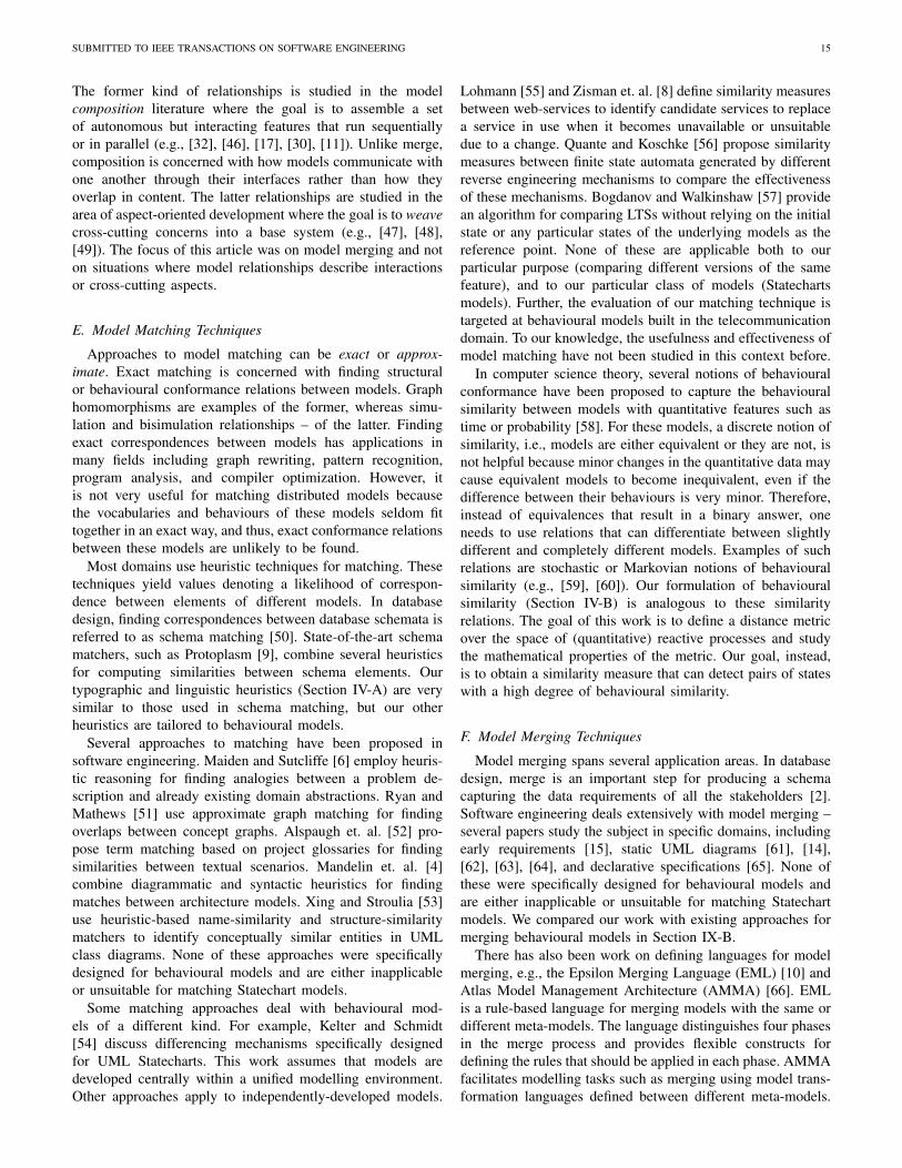
Variables ``subscriber'', ``participant'', and ``callee'' are port variables.A label ``p?e'' on a transition indicates that the transition is triggered by event ``e'' sent from port ``p''.
These variants are examples of DFC ``feature boxes'', which can be instantiated in the ``source zone'' or the ``target zone''. Feature boxes instantiated in the source zone apply to all outgoing calls of a customer, and those instantiated in the target zone apply to all their incoming calls. The conditions ``zone = source'' and ``zone = target'' are used for distinguishing the behaviours of feature boxes in different zones.
Fig. 1. Simplified variants of the call logger feature.
merging variant feature specifications described as hierarchicalstate machines. Merging combines structural and semanticinformation present in the state machine models and ensuresthat their behavioural properties are preserved. In our work,we separate identification of model relationships from modelintegration by providing independent Match and Merge op-erators. Our Match operator includes heuristics for findingterminological, structural, and semantic similarities betweenmodels. Our Merge operator parameterizes variabilities be-tween the input models so that their behavioural propertiesare guaranteed to be preserved in their merge. We report ontool support for our Match and Merge operators, and illustrateand evaluate our work by applying these operators to a set oftelecommunication features built by AT&T.
A. Motivating ExampleDomain. We motivate our work with a scenario for maintain-ing variant feature specifications at AT&T. These executablespecifications are modules within the Distributed Feature Com-position (DFC) architecture [17], [18], and form part of aconsumer voice-over-IP service [19]. The features are specifiedas hierarchical state machines.
One feature of the voice-over-IP service is “call logging”,which makes an external record of the disposition of a callallowing customers to later view information on calls theyplaced or received. At an abstract level, the feature works asfollows: It first tries to setup a connection between the callerand the callee. If for any reason (e.g., the caller hanging upor the callee not responding), a connection is not established,a failure is logged; otherwise, when the call is completed,information about the call is logged.
Initially, the functionality was designed only for basic phonecalls, for which logging is limited to the direction of a call,
P1 After a connection is set up, a successful call will be loggedif the subscriber or the participant sends Accept
P2 After a connection is set up, a voicemail will be loggedif the call is redirected to the voicemail service
Fig. 2. Sample behavioural properties of the models in Figure 1: P1represents an overlapping behaviour, and P2 – a non-overlapping one.
the address location where a call is answered, success orfailure of the call, and the duration if it succeeds. Later,a variant of this feature was developed for customers whosubscribe to the voicemail service. Incoming calls for thesecustomers may be redirected to a voicemail resource, andhence, the log information should include the voicemail statusas well. Figure 1 shows simplified views of the basic andvoicemail variants of this feature. To avoid clutter, we combinetransitions that have the same source and target states usingthe disjunction (OR) operator.
In the DFC architecture, telecom features may come inseveral variants to accommodate different customers’ needs.The development of these variants is often distributed acrosstime and over different teams of people, resulting in theconstruction of independent but overlapping models for eachfeature. For example, consider the two properties described inFigure 2. Property P1 holds in both variants shown in Figure 1because both can log a successful call: P1 holds via the pathfrom s4 to s6 in the basic variant, and via the path from t4 tot6 in voicemail. This property represents a potential overlapbetween the behaviours of these variants. In contrast, propertyP2 only holds in voicemail (via the path from t4 to t8) butnot in basic. This property illustrates a behavioural variationbetween the variants shown in Figure 1.
Goal. To reduce the high costs associated with verifying and

SUBMITTED TO IEEE TRANSACTIONS ON SOFTWARE ENGINEERING 3
maintaining independent models, it is desirable to consolidatethe variants of each feature into a single unified model.To do this, we need to identify correspondences betweenvariant models and merge these models with respect to theircorrespondences.
B. Contributions of this article
Match and Merge are recurring problems arising in differ-ent contexts. Our motivating example illustrates one of themany applications of these operators. Implementing Match andMerge involves answering several questions. Particularly, whatcriteria should we use for identifying correspondences betweendifferent models? How can we quantify these criteria? Howcan we construct a merge given a set of models and theircorrespondences? How can we distinguish between shared andnon-shared parts of the input models in their merge? Whatproperties of the input models should be preserved by theirmerge? In this article, we address these questions for modelsexpressed as hierarchical state machines. The contributions ofthis article are as follows:• A versatile Match operator for hierarchical state ma-
chines. Our Match operator uses a range of heuristicsincluding typographic and linguistic similarities betweenthe vocabularies of different models, structural similari-ties between the hierarchical nesting of model elements,and semantic similarities between models based on aquantitative notion of behavioural bisimulation. We applyour Match operator to a set of telecom feature speci-fications developed by AT&T. Our evaluation indicatesthat the approach is effective for finding correspondencesbetween real-world models.
• A Merge operator for hierarchical state machines.We provide a procedure for constructing behaviour-preserving merges that also respect the hierarchical struc-turing of the input models. We use this Merge operatorfor combining variant telecom features from AT&T basedon the relationships computed by our Match operator be-tween the features. We provide an implementation of ourMerge operator as part of a tool, named TReMer+ [20].
The rest of this article is organized as follows. Section IIprovides an overview of our Match and Merge operators. Sec-tion III outlines our assumptions and fixes notation. Section IVintroduces our Match operator, and Section V – our Mergeoperator. Section VI describes tool support for the two oper-ators. Section VII presents an evaluation of effectiveness forthe Match operator, and Section VIII assesses the soundnessof the Merge operator. Section IX compares our contributionswith related work and discusses the results presented in thisarticle. Finally, Section X concludes the article.
II. OVERVIEW OF OUR APPROACH
Figure 3 provides an overview of our framework for in-tegrating variant feature specifications. The framework hastwo main steps. In the first step, a Match operator is usedto find relationships between the input models. In the secondstep, an appropriate Merge operator is used to combine themodels with respect to the relationships computed by Match.
Fig. 3. A framework for integrating variant feature specifications.
The novelty of this framework is the explicit distinctionbetween the identification of model relationships and modelintegration. The Match and Merge operators in this frameworkare independent, but they are used synergistically to allow usto hypothesize alternative ways of combining models, and tocompute the result of merge for each alternative.
Our ultimate goal is to provide automated tool supportfor the framework in Figure 3. Among these two operators,Match has a heuristic nature. Since models are developedindependently, we can never be entirely sure about how thesemodels are related. At best, we can find heuristics that canimitate the reasoning of a domain expert. In our work, we usetwo types of heuristics: static and behavioural. Static heuristicsuse structural and textual attributes, such as element names,for measuring similarities. For the models in Figure 1, staticheuristics would suggest a number of good correspondences,e.g., the pairs (s6, t6), and (s7, t7); however, these heuristicswould miss several others, including (s3, t3), (s3, t2) and(s4, t4). These pairs are likely to correspond not because theyhave similar static characteristics, but because they exhibitsimilar dynamic behaviours. Our behavioural heuristic can findthese pairs.
To obtain a satisfactory correspondence relation, we use acombination of static and behavioural heuristics. Our Matchoperator produces a correspondence relation between statesin the two models. For the models in Figure 1, it may yieldthe correspondence relation shown in Figure 8(b). Becausethe approach is heuristic, the relation must be reviewed by adomain expert and adjusted by adding any missing correspon-dences and removing any spurious ones. In our example, thefinal correspondence relation approved by a domain expert isshown in Figure 8(c).
Unlike matching, merging is not heuristic, and is almostentirely automatable. Given a pair of models and a correspon-dence relation between them, our Merge operator automati-cally produces a merge that:
1) preserves the behavioural properties of the input models.Figure 9 shows the merge of the models of Figure 1with respect to the relation in Figure 8(c). This mergeis behaviour-preserving. That is, any behaviour of theinput models is preserved in the merge model (eitherthrough shared or non-shared behaviours). For example,the property P1 in Figure 2 that shows an overlappingbehaviour between the models in Figure 1 is preservedin the merge as a shared behaviour (denoted by the pathfrom state (s4, t4) to (s6, t6)).

SUBMITTED TO IEEE TRANSACTIONS ON SOFTWARE ENGINEERING 4
2) distinguishes between shared and non-shared behavioursof the input models by attaching appropriate guardconditions to non-shared transitions. In the merge, non-shared transitions are guarded by boldface conditionsrepresenting the models they originate from. For exam-ple, the property P2 in Figure 2 which holds over thevoicemail variant but not over the basic, is representedas a parameterized behaviour in the merge (denoted bythe transition from (s4, t4) to t8), and is preserved onlywhen its guard holds.
3) respects the hierarchical structure of the input models,providing users with a merge that has the same concep-tual structure as the input models.
III. ASSUMPTIONS AND BACKGROUND
The Statechart language [21] is a common notation for de-scribing hierarchical state machines and is a de-facto standardfor specifying intra-object behaviours of software systems.Below, the syntax of this language is formalized [22].
Definition 1 (Statecharts): A Statecharts model is a tuple(S, s, <h, E, V,R), where S is a finite set of states; s ∈ S is aninitial state; <h is a partial order defining the state hierarchytree (or hierarchy tree, for short); E is a finite set of events; Vis a finite set of variables; and R is a finite set of transitions,each of which is of the form 〈s, e, c, α, s′, prty〉, where s, s′ ∈S are the transition’s source and target, respectively, e ∈ E isthe triggering event, c is an optional predicate over V , α isa sequence of zero or more actions that generate events andassign values to variables in V , and prty is a number denotingthe transition’s priority.
We write a transition 〈s, e, c, α, s′, prty〉 as se[c]/α−→ prty s
′.Each state in S can be either an atomic state or a superstate.The hierarchy tree <h defines a partial order on states withthe top superstate as root and the atomic states as leaves. Forexample, in the Statechart of the basic call logger model inFigure 1, s0 is the root, s2 through s7 are leaves, and s1 isneither. The set s of initial states is {s0, s1, s2}. The set Eof events is {setup, Ack, Accept,Reject, TearDown}, and the setV of variables is {callee, zone, participant, subscriber}. The onlyactions in Figure 1 are callee=participant and callee=subscriber.These actions assign values participant and subscriber to thevariable callee, respectively.
Implementations of the Statechart language differ on howthey define the semantics of inter- and intra-machine com-munication and parallelism, and how they resolve non-determinism in the language [22]. The implementation ofthe AT&T features is based on a Statechart dialect, calledECharts [23], and makes the following choices regarding theseissues:• Inter- and intra-machine communication. ECharts
does not permit actions generated by a transition ofa Statechart to trigger other transitions of the sameStatechart [24]. That is, an external event activates atmost one transition, not a chain of transitions. Therefore,notions of macro- and micro-steps coincide in ECharts.
• Parallelism. ECharts uses parallel states with interleavedtransition executions [23], and can be translated to the
x!
x y
y!a b
xy
x!y
x!y!
xy!a b
b!
a
Fig. 4. Resolving AND-states (parallel states) in ECharts.
s1
a
s0a
a
b
c
s!0
cs′1
(a) (b)s2
s3
bs′2
Fig. 5. (a) Prioritizing transitions to eliminate non-determinism in ECharts:Transition s1 → s3 has higher priority than transition s0 → s2, and (b) theflattened form of the Statecharts in (a).
above formalism using the interleaving semantics of [22].A simple example of this translation is shown in Figure 4.
• Non-determinism. In Statecharts, it may happen that astate and some of its proper descendants have outgoingtransitions on the same event and condition, but to dif-ferent target states. For example, in Figure 5(a), states s0and s1 have transitions labelled a to two different states,s2 and s3, respectively. This makes the semantics of thisStatechart model non-deterministic because on receiptof the event a, it is not clear which of the transitions,s0 → s2 or s1 → s3, should be taken. In ECharts,transitions with the same event and condition can bemade deterministic by assigning them globally-orderedpriorities (using prty). For example, in Figure 5(a), itis assumed that the inner transitions have higher priorityover the outer transitions, and hence, on receipt of a, thetransition from s1 to s3 is activated. The models shownin Figure 1 are already deterministic, i.e., any externalevent triggers at most one transition in them. Thus, nofurther prioritization is required.
Note that our Matching and Merging techniques are gen-eral and can be applied to various Statechart dialects. Inorder to demonstrate that the Merge operator is semantic-preserving, one needs to explicitly identify how the abovesemantic variation points are resolved in a particular Statechartimplementation. Our proof for semantic preservation of Merge(see Appendix XI-C) can carry over to other dialects.
In addition, we make the following assumptionson how behavioural models are developed inour context. Let M1 = (S1, s, <
1h, E1, V1, R1) and
M2 = (S2, t, <2h, E2, V2, R2) be Statechart models.
• We assume that the sets of events, E1 and E2, are drawnfrom a shared vocabulary, i.e., there are no name clashes,and no two elements represent the same concept. Thisassumption is reasonable for design and implementationmodels because events and variables capture observablestimuli, and for these, a unified vocabulary is oftendeveloped during upstream lifecycle activities. Note thatthis assumption is also valid for variables in V1 and V2
SUBMITTED TO IEEE TRANSACTIONS ON SOFTWARE ENGINEERING 5
CorrespondenceRelation ( )!
+ Translation
Threshold
M1,M2
Static Matching ( )
Behavioural Matching ( )
S
B
Typographic Matching ( )
Linguistic Matching ( )
Depth Matching ( )
TG
D
Match
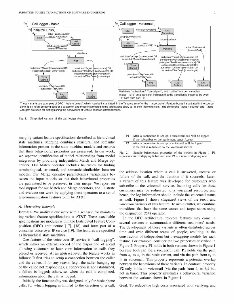
Fig. 6. Overview of the Match operator.
that appear in the guard conditions, i.e., the environmental(input) variables.
• Since M1 and M2 describe variant specifications of thesame feature, they are unlikely to be used together inthe same configuration of a system, and hence, unlikelyto interact with one another. Therefore, we assume thatactions of either M1 or M2 cannot trigger events in theother model. For example, the only actions in the State-chart in Figure 1 are callee=participant and callee=subscriber.These actions do not cause any interaction between theStatechart models in Figure 1. Hence, the models inFigure 1 are non-interacting. For a discussion on dis-tinctions between models with interacting vs. overlappingbehaviours, see Section IX.
IV. MATCHING STATECHARTS
Our Match operator (Figure 6) uses a hybrid approachcombining static matching, S (Section IV-A), and behaviouralmatching, B (Section IV-B). Static matching is independentof the Statechart semantics and combines typographic andlinguistic similarity degrees between state names, respectivelydenoted T and G, with similarity degrees between statedepths in the models’ hierarchy trees, denoted D. Behaviouralmatching (B) generates similarity degrees between states basedon their behavioural semantics. Each matching is defined as atotal function S1 × S2 → [0..1], assigning a normalized valueto every pair (s, t) ∈ S1×S2 of states. The closer a degree isto one, the more similar the states s and t are (with respect tothe similarity measure being used). We aggregate the static andbehavioural heuristics to generate the overall similarity degreesbetween states (Section IV-C). Given a similarity threshold, wecan then determine a correspondence relation ρ over the statesof the input models (Section IV-C).
A. Static Matching
Static matching, S, is calculated by combining typographic(T ), linguistic (G), and depth (D) similarities. In this article,we use the following formula for the combination:
S = 4·max(T ,G)+D5
The typographic, linguistic and depth heuristics are describedbelow.
Typographic Matching (T ) assigns a value to every pair
(s, t) by applying the N-gram algorithm [25] to the namelabels of s and t. Given a pair of strings, this algorithmproduces a similarity degree based on counting the numberof their identical substrings of length N. We use a genericimplementation of this algorithm with trigrams (i.e., N = 3).For example, the result of trigram matching for some of thename labels of the states in Figure 1 is as follows:
trigram(“Wait”, “Pending”) = 0.0trigram(“Log Success”, “Log Failure”) = 0.21trigram(“Log Success”, “Log Success”) = 1.0trigram(“Link Callee”, “Link Participant”) = 0.18
Linguistic Matching (G) measures similarity between namelabels based on their linguistic correlations, to assign a nor-malized similarity value to every pair of states. We employthe freely available WordNet::Similarity package [26] for thispurpose. WordNet::Similarity provides implementations for a va-riety of semantic relatedness measures proposed in the NaturalLanguage Processing (NLP) literature. In our work, we use thegloss vector measure [27] – an adaptation of the popular cosinesimilarity measure [28] used in data mining for computing asimilarity degree between two words based on the availabledictionary and corpus information. For a given pair of words,the gloss vector measure is a normalized value in [0..1].
In many cases, the name labels whose relatedness is beingmeasured are phrases or short sentences, e.g., “Log Success”and “Log Failure” in Figure 1. In these cases, we need anaggregate measure that computes degrees for name labelsexpressed as sentences or phrases. To this end, we use a simplemeasure from natural language processing [25], describedbelow.
We treat each name label as a set of words (which impliesthat the parts of speech of the words in the name labels areignored) and compute the gloss vector degrees for all wordpairs of the input labels. We then find a matching betweenthe words of the input labels such that the sum of the degreesis maximized. This optimization problem is easily cast intothe maximum weighted bipartite graph matching problem, alsoknown as the assignment problem [29]. The nodes on each sideof the bipartite graph are the words in one of the input labels.There is an edge e with weight w between word x of the firstinput label and word y of the second input label if the degreeof relatedness between x and y is w. The result of maximumweighted bipartite matching is a set of edges e1, . . . , ek suchthat no two edges have the same node (i.e., word) as anendpoint, and the sum
∑ki=1 weight(ei) is maximal. If the
input name labels are for a pair of states (s, t), linguisticsimilarity between s and t is given by the following:
G(s, t) =2 ·∑k
i=1 weight(ei)N1 +N2
where N1 and N2 are the number of words in each of the twoname labels being compared.
As an example, suppose we want to compute a degree ofsimilarity for the labels “system busy” and “component inuse”. Figure 7 shows the pairwise similarity matrix for thewords of the two labels, computed using the gloss vector

SUBMITTED TO IEEE TRANSACTIONS ON SOFTWARE ENGINEERING 6
component in usesystem 0.45 0.16 0.36busy 0.18 0.1 0.37
Fig. 7. Similarity degrees between words in name labels expressed as phrases.
measure. The maximal weight matching is achieved when“system” is matched to “component” and “busy” is matched to“use”. This gives us a value of 2×(0.45+0.37)/(2+3) ≈ 0.33.
Depth Matching (D) uses state depths to derive a similarityheuristic for models that are at the same level of abstraction.This captures the intuition that states at similar depths are morelikely to correspond to each other and is computed as follows:
D(s, t) = 1− |depth(s)−depth(t)|max(depth(s),depth(t))
where depth(s) and depth(t) are respectively the positionof states s and t in the state hierarchy tree orderings < oftheir corresponding input models. For example, in Figure 1,depth(s2) is 2 and depth(t1) is 1, and D(s2, t1) = 0.5.
B. Behavioural Matching
Behavioural matching (B) provides a measure of similaritybetween the behaviours of different states. Our behaviouralmatching technique draws on the notion bisimilarity betweenstate machines [30]. Bisimilarity provides a natural way tocharacterize behavioural equivalence. Bisimilarity is a recur-sive notion and can be defined in a forward and backwardway [31]. Two states are forward bisimilar if they cantransition to (forward) bisimilar states via identically-labelledtransitions; and are (forward) dissimilar otherwise.
Dually, two states are backward bisimilar if they can betransitioned to from (backward) bisimilar states via identically-labelled transitions; and are (backward) dissimilar otherwise.
Bisimilarity relates states with precisely the same set ofbehaviours, but it cannot capture partial similarities. For exam-ple, states s4 and t4 in Figure 1 transit to (forward) bisimilarstates s7 and t7, respectively, with transitions labelled partic-ipant?Reject[zone=source], participant?TearDown[zone=source], sub-scriber?Reject[zone=target], and subscriber?TearDown[zone=target].However, despite their intuitive similarity, s4 and t4 are dissim-ilar because their behaviours differ on a few other transitions,e.g., the one labelled redirectToVoicemail[zone=target].
Instead of considering pairs of states to be either bisimilaror dissimilar, we introduce an algorithm for computing a quan-titative value measuring how close the behaviours of one stateare to those of another. Our algorithm iteratively computes asimilarity degree for every pair (s, t) of states by aggregatingthe similarity degrees between the immediate neighbors of sand those of t. By neighbors, we mean either successor/childstates (forward neighbors) or predecessor/parent states (back-ward neighbors) depending on which bisimilarity notion isbeing used. The algorithm iterates until either the similaritydegrees between all state pairs stabilize, or a maximum numberof iterations is reached.
In the remainder of this section, we describe the algorithmfor the forward case. The backward case is similar. We use thenotation s a→ s′ to indicate that s′ is a forward neighbor of s.That is, s has a transition to s′ labelled a, or s′ is child of swhere a is a special label called child. Treating children statesas neighbors allows us to propagate similarities from childrento their parents and vice versa.
We denote by Bi(s, t) the degree of similarity betweenstates s and t after the ith iteration of the matching algorithm.Initially, all states of the input models are assumed to bebisimilar, so B0(s, t) is 1 for every pair (s, t) of states. Usersmay override the default initial values, for example, assigningzero to those tuples that they believe would not correspond toeach other. This enables users to apply their domain expertiseduring the matching process. Since behavioural matching isiterative, user input gets propagated to all tuples and can henceinduce an overall improvement in the results of matching.
For proper aggregation of similarity degrees between states,our behavioural matching requires a measure for comparingtransition labels. A transition label is made up of an event and,optionally, a condition and an action. We compare transitionlabels using the N-gram algorithm augmented with somesimple semantic heuristics. This algorithm is suitable becauseof the assumption that a shared vocabulary for observablestimuli already exists. The algorithm assigns a similarity valueL(a, b) in [0..1] to every pair (a, b) of transition labels.
Having described the initialization data (B0) and transitionlabel comparison (L), we now describe the computation ofB. For every pair (s, t) of states, the value of Bi(s, t) iscomputed from (1) Bi−1(s, t); (2) similarity degrees betweenthe forward neighbors of s and those of t after step i− 1; and(3) comparison between the labels of transitions relating s andt to their forward neighbors.
We formalize the computation of Bi(s, t) as follows. Letsa→ s′. To find the best match for s′ among the forward neigh-
bors of t, we need to maximize the value L(a, b)× Bi−1(s′, t′)where t b→ t′.
The similarity degrees between the forward neighbors of sand their best matches among the forward neighbors of t afteri− 1th iteration is computed by
X =∑s
a→s′max
tb→t′L(a, b)× Bi−1(s′, t′)
And the similarity degrees between the forward neighbors oft and their best matches among the forward neighbors of safter iteration i− 1 are computed by
Y =∑t
a→t′max
sb→s′L(a, b)× Bi−1(s′, t′)
We denote the sum of X and Y by Sumi(s, t).The value of Bi(s, t) is computed by first normalizing
Sumi(s, t) and then computing its average with Bi−1(s, t):
Bi(s, t) = 12
` Sumi(s,t)|succ(s)|+|succ(t)| + B
i−1(s, t)´
In the above formula, |succ(s)| and |succ(t)| are the numberof forward neighbors of s and t, respectively. The larger the
SUBMITTED TO IEEE TRANSACTIONS ON SOFTWARE ENGINEERING 7
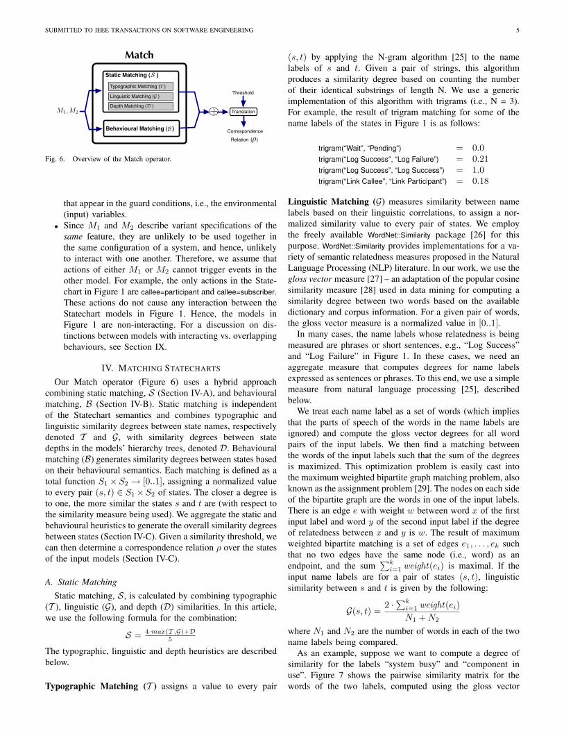
s0 s1 s2 s3 s4 s5 s6 s7
t0 .87 .63 .54 .03 .08 .07 .57 .58t1 .48 .70 .92 .17 .17 .26 .20 .23t2 .08 .18 .17 .65 .30 .31 .31 .29t3 .07 .19 .17 .66 .30 .32 .30 .30t4 .07 .15 .17 .23 .64 .30 .30 .30t5 .08 .15 .25 .22 .24 1.0 .04 .28t6 .58 .45 .17 .22 .30 .30 1.0 .63t7 .56 .45 .17 .22 .31 .28 .62 1.0t8 .55 .45 .17 .22 .30 .35 .62 .62
(a) Combined C matching results for the modelsin Figure 1.
(s0, t0), (s2, t1), (s3, t2), (s3, t3), (s4, t4), (s5, t5), (s6, t6),(s7, t7), (s1, t0), (s1, t1), (s6, t7), (s6, t8), (s7, t6), (s7, t8)
(b) A correspondence relation ρ.
(s0, t0), (s4, t4), (s2, t1), (s5, t5), (s3, t2), (s6, t6), (s3, t3), (s7, t7)
(c) ρ after revisions of Section IV-C and sanity checks of Section V-A.
Fig. 8. Results of matching for call logger.
Bi(s, t), greater is the similarity of the behaviours of s andt. For backward behavioural matching, we perform the abovecomputation for states s and t, but consider their backwardneighbours instead of their forward neighbours.
The above computation is performed iteratively until thedifference between Bi(s, t) and Bi−1(s, t) for all pairs (s, t)becomes less than a fixed ε > 0. If the computation does notconverge, the algorithm stops after some predefined maximumnumber of iterations. Finally, we compute behavioural similar-ity, B, as the maximum of forward behavioural and backwardbehavioural matching.
C. Combining Similarities and Translating them to Corre-spondences
To obtain the overall similarity degrees between states, weneed to combine the results from different heuristics. Thereare several approaches to this, including linear and nonlinearaverages, and machine learning techniques. Learning-basedtechniques have been shown to be effective when propertraining data is available [4]. Since such data was not presentfor our case study, our current implementation uses a simpleapproach based on linear averages. To produce an overallcombined measure, denoted C, we take an average of B withstatic matching, S (described in Section IV-A). Figure 8(a)illustrates C for the models in Figure 1.
To obtain a correspondence relation between input Stat-echart models M1 and M2, the user sets a threshold fortranslating the overall similarity degrees into a relation ρ.Pairs of states with similarity degrees above the threshold areincluded in ρ, and the rest are left out. In our example, if weset the threshold value to 60%, we obtain the correspondencerelation ρ shown in Figure 8(b). Since matching is a heuristic
process, ρ should be reviewed and, if necessary, adjusted bythe user. For example, in Figure 1, since states s6 and s7of basic and states t6, t7 and t8 of voicemail do not haveany outgoing transitions, there is a high degree of (forward)behavioural similarity between them, and hence, all the pairs(s6, t6), (s6, t7), (s6, t8), (s7, t6), (s7, t7), and (s7, t8) appearin ρ in Figure 8(b). Among these pairs, however, only (s6, t6)and (s7, t7) are valid correspondences according to the user.We assume the user would remove the rest of the pairs fromρ. As we discuss in Section V-A, the relation ρ may need tobe further revised before merging to ensure that the resultingmerged model is well-formed.
V. MERGING STATECHARTS
In this section, we describe our Merge operator for State-charts. The input to this operator is a pair of Statechart modelsM1 and M2, and a correspondence relation ρ. The output isa merged model if ρ satisfies certain sanity checks (discussedin Section V-A). These checks ensure that merging M1 andM2 using ρ results in a well-formed (i.w., structurally sound)Statechart model. If the checks fail, a subset of ρ violating thechecks is identified.
A. Sanity Checks for Correspondence Relations
To produce structurally sound merges, we need to ensurethat ρ passes certain sanity checks before applying the Mergeoperator:
1) The initial states of the input models should correspondto one another. If ρ does not match s to t, we add to theinput models new initial states s′ and t′ with transitionsto the old ones. We then simply add the tuple (s′, t′)to ρ. Note that we can lift the behavioural properties ofthe models with the old initial states to those with thenew initial states. For example, instead of evaluating atemporal property p at s (respectively t), we check AXpat s′ (respectively t′), where AX denotes the universalnext-time operator – we borrow it from the commonly-used temporal logic CTL [32].
2) The correspondences in ρ must respect the input models’hierarchy trees. That is, ρ must satisfy the followingconditions for every (s, t) ∈ ρ:
a) (monotonicity) If ρ relates a proper descendant ofs (respectively t) to a state x in M2 (respectivelyM1), then x must be a proper descendant of t(respectively s).
b) (relational adequacy) Either the parent of s isrelated to an ancestor of t, or the parent of t isrelated to an ancestor of s by ρ.
Monotonicity ensures that ρ does not relate an ancestorof s to t (respectively t to s) or to a child thereof. Re-lational adequacy ensures that ρ does not leave parentsof both s and t unmapped; otherwise, it would not beclear which state should be the parent of s and t in themerge. Note that descendant, ancestor, parent, and childare all with respect to each model’s hierarchy tree, <h.
Pairs in ρ that violate any of the above conditions arereported to the user. In our example, the relation shown in

SUBMITTED TO IEEE TRANSACTIONS ON SOFTWARE ENGINEERING 8
(Link Callee, Link Subscriber)
(Link Callee, Link Participant)
(Wait, Pending)
(Timer Started, Timer Started)
(Log Failure, Log Failure)
(Log Success, Log Success)
setup [zone =target]/callee = subscriber
setup [zone=source] /callee=participant
participant?Ack [ID=voicemail]
subscriber?Ack[ID=voicemail]
redirectToVoicemail[zone=target,ID=voicemail]
participant?Reject [zone=source] ORparticipant?Unavail [zone=source, ID=voicemail]OR
participant?TearDown [zone=source] ORsubscriber?Reject [zone=target] OR
subscriber?Unavail [in target-zone, ID=voicemail] ORsubscriber?TearDown [zone=target]
participant?TearDown ORsubscriber?TearDown
participant?Accept [zone=source] ORsubscriber?Accept [zone=target]
Log Voicemail
(s0, t0)
callee?Ack[ID=basic]
callee?Ack[ ID=basic]
Call logger - (basic, voicemail)
(Start, Start)
Initialize Linkss1
(s2, t1)(s3, t2)
(s3, t3)
(s4, t4)
(s5, t5)
(s6, t6) (s7, t7) t8
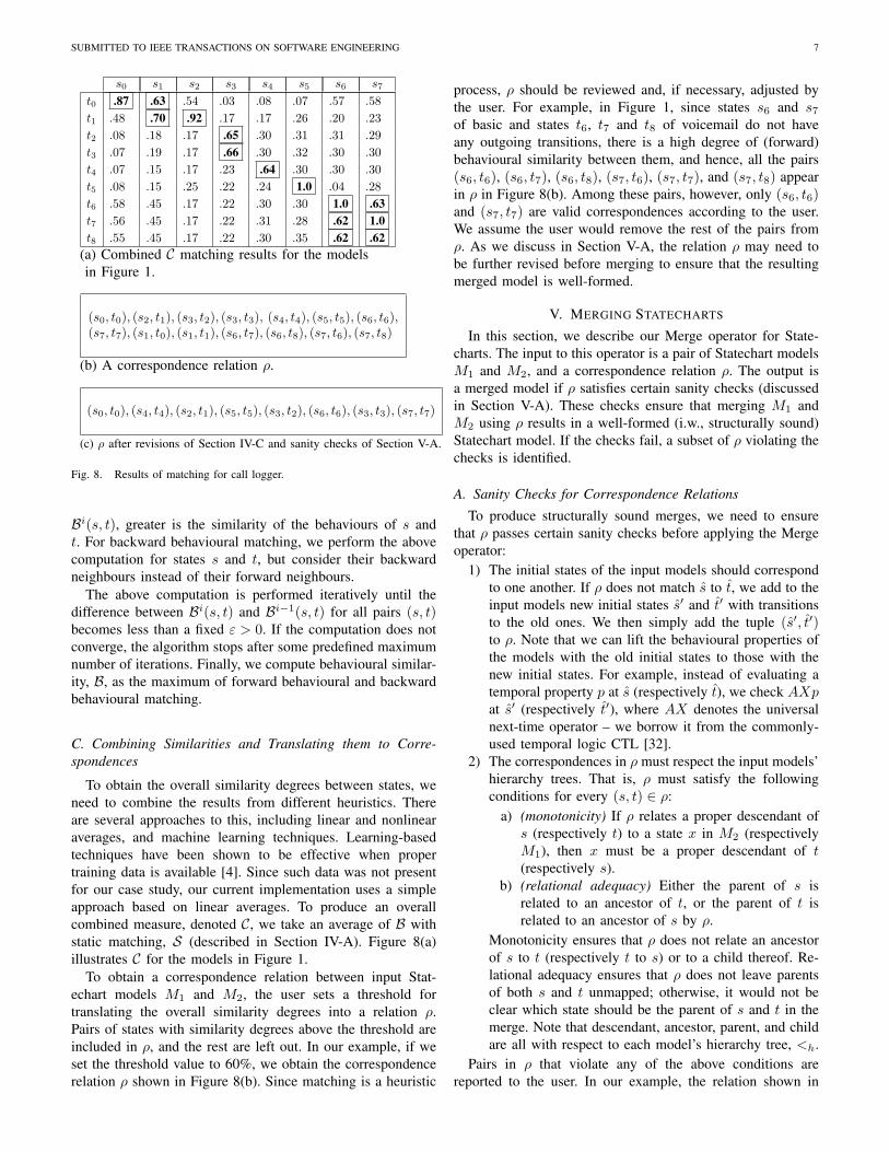
Fig. 9. Resulting merge for the call logger variants in Figure 1.
Figure 8(b) has three monotonicity violations: (1) s0 and itschild s1 are both related to t0; (2) t0 and its child t1 are bothrelated to s1; and (3) s1 and its child s2 are both related to t1.Our algorithm reports {(s0, t0), (s1, t0)}, {(s1, t0), (s1, t1)},and {(s1, t1), (s2, t1)} as conflicting sets. Suppose that theuser addresses these conflicts by eliminating (s1, t0) and(s1, t1) from ρ. The resulting relation, shown in Figure 8(c),passes all sanity checks and can be used for merge.
B. Merge Construction
Let M1 and M2 be Statechart models. To merge them,we first need to identify their shared and non-shared partswith respect to ρ. A state x is shared if it is related tosome state by ρ, and is non-shared otherwise. A transitionr = 〈x, a, c, α, y, prty〉 is shared if x and y are respectivelyrelated to some x′ and y′ by ρ, and further, there is a transitionr′ from x′ to y′ whose event is a, whose condition is c, whosepriority is prty , and whose action is α′ such that either α = α′,or α and α′ are independent. A pair of actions α and α′ areindependent if executing them in either order results in thesame system behaviour [32]. For example, z = x and y = xare two independent actions, but x = y+ 1 and z = x are notindependent. r is non-shared otherwise.
The goal of the Merge operator is to construct a modelthat contains shared behaviours of the input models as normalbehaviours and non-shared behaviours as variabilities. To rep-resent variabilities, we use parameterization [33]: Non-sharedtransitions are guarded by conditions denoting the transitions’origins, before being lifted to the merge. Non-shared states canbe lifted without any provisions – these states are reachableonly via non-shared (and hence, guarded) transitions.
Below, we describe our procedure for constructing a merge.We denote by M1 +ρ M2 = (S+, s+, <
+h , E+, V+, R+) the
merge of M1 and M2 with respect to ρ – a correspondencerelation between these models.• States and Initial State. (S+ and s+) The set S+ of
states of M1 +ρ M2 has one element for each tuple in
tss� t�
(s, t)(s�, t�)=⇒
tss�
(s, t)
=⇒ s�
ss� t� (s�, t�)=⇒
s ss�
=⇒ss�
(a) (b)
(c) (d)
Fig. 10. Merging different state hierarchy patterns.
ρ and one element for each state in M1 and M2 that isnon-shared. The initial state of M1 +ρ M2, s+, is thetuple (s, t).
• Events and Variables. (E+ and V+) The set E+ ofevents of M1 +ρ M2 is the union of those of M1 andM2. The set V+ of variables of M1 +ρM2 is the union ofthose of M1 and M2 plus a reserved enumerated variableID that accepts values M1 and M2.
• Hierarchy Tree. (<+h ) The hierarchy tree <+
h
of M1 +ρM2 is computed as follows. Let s be asuperstate in M1 (the case for M2 is symmetric), and lets′ be a child of s.
– if s is mapped to t by ρ,∗ if s′ is mapped to a child t′ of t by ρ, make (s′, t′)
a child of (s, t) in M1 +ρM2 (see Figure 10(a)).∗ otherwise, if s′ is non-shared, make s′ a child of
(s, t) in M1 +ρM2 (see Figure 10(b)).– otherwise, if s is non-shared∗ if s′ is mapped to a state t′ by ρ, make (s′, t′) a
child of s in M1 +ρM2 (see Figure 10(c)).∗ otherwise, if s′ is non-shared, make s′ a child ofs in M1 +ρM2 (see Figure 10(d)).
• Transition Relation. (R+) The transition relation R+
of M1 +ρ M2 is computed as follows. Let r =〈s, a, c, α, s′, prty〉 be a transition in M1 (the case forM2 is symmetric).
– (Shared Transitions) if r is shared, add to R+ atransition corresponding to r with event a, conditionc, action α (if α = α′) or action α;α′ (if α 6= α′),and priority prty .Note that according to the definition of shared tran-sitions, α and α′ are independent. Moreover, basedon our assumptions in Section III, M1 and M2 donot interact, i.e., α does not trigger any transition ofM2, and similarly, α′ does not trigger any transitionof M2. Hence, the order of concatenation of α andα′ in the merged model is not important. Moreover,in case α = α′, we keep only one copy of α in themerge. Hence, the merge does not execute the sameaction twice.
– (Non-shared Transitions) otherwise, if r is non-shared, add to R+ a transition corresponding to rwith event a, condition c ∧ [ID = M1], action α,and priority prty .
As an example, Figure 9 shows the resulting merge for themodels of Figure 1 with respect to the relation ρ in Figure 8(c).

SUBMITTED TO IEEE TRANSACTIONS ON SOFTWARE ENGINEERING 9
The conditions shown in boldface in Figure 9 capture theorigins of the respective transitions. For example, the transitionfrom (s4, t4) to t8 annotated with the condition ID=voicemailindicates a variable behaviour that is applicable only for clientssubscribing to voicemail.
Two points need to be noted about our merge construction:(1) The construction requires that states be either atomic orsuperstates (OR states) – as noted in Section III, parallel states(AND states) are replaced by their semantically equivalentnon-parallel structures before merge. To keep the structure ofthe merged model as close as possible to the input models,non-shared parallel states can be exempted from this replace-ment when all of their descendants are non-shared as well.Such parallel states (and all of their descendants) can be liftedverbatim to the merge. (2) Our definition of shared transitionsis conservative in the sense that it requires such transitionsto have identical events, conditions, and priorities in bothinput models. This is necessary in order to ensure that mergesare behaviourally sound and deterministic. However, sucha conservative approach may result in redundant transitionswhich arise due to logical or unstated relationships between theevents and conditions used in the input models. For example,in Figure 9, the transitions from (s2, t1) to (s3, t2) and to(s3, t3) fire actions callee = subscriber and callee=participant,respectively. Thus, in state (s3, t3), the value of callee is equalto participant, and in state (s3, t2), it is equal to subscriber. Thisallows us to replace the event callee?Ack[ID=basic] on transitionfrom (s3, t2) to (s4, t4) by subscriber?Ack[ID=basic], and mergethe two out-going transitions from (s3, t2) into one transitionwith label subscriber?Ack. Similarly, the two transitions from(s3, t3) to (s4, t4) can be merged into one transition with labelparticipant?Ack. Identifying such redundancies and addressingthem requires human intervention.
VI. TOOL SUPPORT
In this section, we present our implementation of theMatch and Merge operators described in Sections IV and V,respectively.
A. Tool Support for the Match OperatorWe have implemented our Match operator and used it for
the evaluation described in Section VII. Our implementationtakes Statechart models stored as XML files and computessimilarity values for static matching, behavioural matching andtheir combinations. It can further generate a binary correspon-dence relation for a given threshold value. This relationship,after revisions and adjustments by the user, can be used tospecify the model mappings in our merge tool described inSection VI-B.
Our Match tool consists of approximately 2.6K lines ofJava code, of which 1K implement N-gram and linguisticmatching [25], and are borrowed from existing open-sourceimplementations. Of the remaining 1.6K lines of code, 1Kimplement our depth and behavioural matching techniques,and the rest is the parser for state machine data representedas XML files and the code for interacting with the userthrough the command line. The Match tool is available athttp://se.cs.toronto.edu/index.php/MatchTool/.
B. Tool Support for the Merge Operator
We have implemented our Merge operator as part of atool called TReMer+ [20]. TReMer+ additionally providesimplementations for the structural merge approach in [15] andthe consistency checking approach in [34] which we do notdiscuss here. TReMer+ consists of roughly 15K lines of Javacode, of which 8.5K lines implement the user interface, 5.5Klines implement the tool’s core functionality (model merging,traceability, and serialization), and 1000 lines implement theglue code for interacting with an external consistency rulechecker. The Merge operator described in this article accountsfor approximately 1200 lines of the code. We have usedTReMer+ for merging the sets of variant Statechart modelsobtained from AT&T. Our tool and the material for the casestudies that we have conducted using it are available athttp://se.cs.toronto.edu/index.php/TReMer+.
The main characteristic of TReMer+ is that it enables de-velopers to explicitly specify the relationships between modelsand treat these relationships as first-class artifacts in the mergeprocess [1]. Such a treatment makes it possible to hypothesizealternative relationships between models and study the resultof merge for each alternative. The alternatives can be identifiedmanually or be based on the results of the automated matcherdescribed in Section VI-A.
Figure 11 shows how our Merge operator is applied inTReMer+: Given a pair of variant models, the user firstdefines one or several alternative relationships between themodels. The models and a selected relationship are then usedto compute a merge. The resulting merge is presented to theuser for further analysis. This may lead to the discovery ofnew element mappings or the invalidation of some of theexisting ones. The user may then want to start a new iterationby revising the relationship and executing the subsequentactivities. In this article, the preliminary relationships used toinitiate the iterative process of Figure 11 were computed byour Match operator.
Define/Revise Relationship(s)
Variant Models
Compute MergeRelationship
Merged View
User
Fig. 11. Overview of model merging with TReMer+
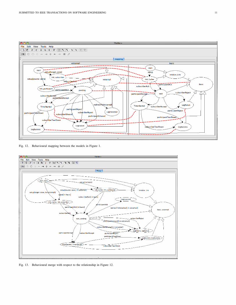
In the remainder of this section, we illustrate our tool usingthe variant models in Figure 1. First the input models arespecified using the tool’s graphical editing environment. Theuser can then define a relationship using the tool’s mappingwindow, a snapshot of which is shown in Figure 12. In thiswindow, the input models are shown side-by-side. A statemapping is established by first clicking on a state of the modelon the left and then on a state of the model on the right.To show the desired correspondences, we have added to thescreenshot a set of dashed lines indicating the related states.
SUBMITTED TO IEEE TRANSACTIONS ON SOFTWARE ENGINEERING 10
The relationship shown in the snapshot is the one given earlierin Figure 8(c). Note that the tool represents hierarchical statesusing an arrow with a hollow tail from each sub-state to itsimmediate super-state. For example, the arrow from start toinitialize Link (right side of the snapshot in Figure 12) indicatesthat initialize Link is the immediate super-state of start.
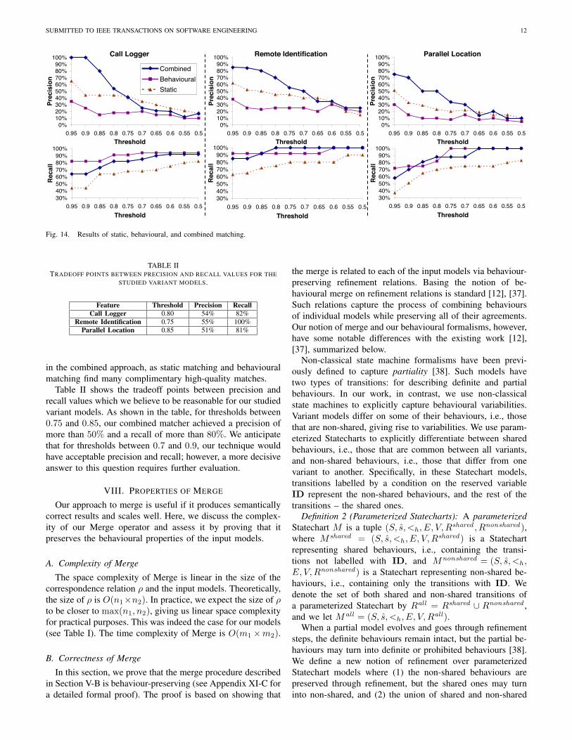
The merge computed by the tool with respect to the rela-tionship defined above is shown in Figure 13. As seen fromthe figure, non-shared behaviours are guarded by conditionsdenoting the input model exhibiting those behaviours.
VII. EVALUATION OF MATCH
Our approach to matching is valuable if it offers a quick wayto identify appropriate matches with reasonable accuracy, inparticular in situations where matches are hard to find by hand,for example, where the models are complex, or the developersare less familiar with them. Here, we present some initial stepsto evaluate our Match operator. First, we discuss its complexityto show that it scales, and then we assess this operator bymeasuring the accuracy of the relationships it produces, whencompared to the assessment of a human expert.
A. Complexity of Match
Let n1 and n2 be the number of states in the inputmodels, and let m1 and m2 be the number of transitions inthese models. The space and time complexities of computingtypographic and linguistic similarity scores between individualpairs of name labels are negligible and bounded by a constant,i.e., the largest value of similarity scores of the state names.Note that since the set of states names is finite and determined,we can compute such a bound. The space complexity ofMatch is then the storage needed for keeping a state similaritymatrix and a label similarity matrix (L in Section IV-B) and isO(n1×n2+m1×m2). The time complexity of static matchingis O(n1×n2) and of behavioural matching – O(c×m1×m2),where c is the maximum allowed number of iterations for thebehavioural matching algorithm.
B. Accuracy of Match
As with all heuristic matching techniques, the results of ourMatch operator should be reviewed and adjusted by users toobtain a desired correspondence relation. In this sense, a goodway to evaluate a matcher is by considering the number ofadjustments users need to make to the results it produces. Amatcher is effective if it neither produces too many incorrectmatches (false positives) nor misses too many correct matches(false negatives).
We use two well-known metrics, namely, precision, andrecall, to capture this intuition. Precision measures quality(i.e., a low number of false positives) and is the ratio of correctmatches found to the total number of matches found. Recallmeasures coverage (i.e., a low number of false negatives) andis the ratio of the correct matches found to the total numberof all correct matches. For example, if our matcher producesthe relationship in Figure 8(b) and the desired relation isshown in Figure 8(c), the precision and recall are 8/14 and8/8, respectively.
TABLE INUMBER OF STATES AND TRANSITIONS OF THE STUDIED VARIANT
MODELS.
Feature Variant I Variant II All Correct# states # transitions # states # transitions Matches
Call Logger 18 40 21 63 11Remote Identification 24 44 19 31 12
Parallel Location 28 71 33 68 16
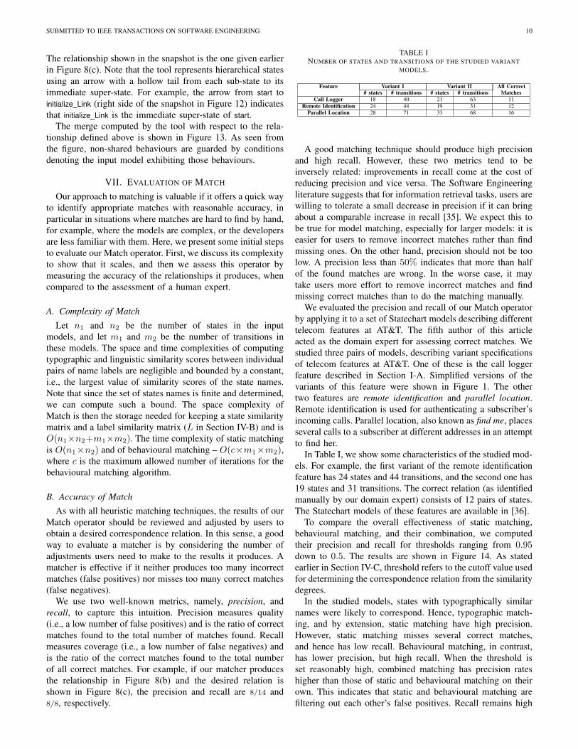
A good matching technique should produce high precisionand high recall. However, these two metrics tend to beinversely related: improvements in recall come at the cost ofreducing precision and vice versa. The Software Engineeringliterature suggests that for information retrieval tasks, users arewilling to tolerate a small decrease in precision if it can bringabout a comparable increase in recall [35]. We expect this tobe true for model matching, especially for larger models: it iseasier for users to remove incorrect matches rather than findmissing ones. On the other hand, precision should not be toolow. A precision less than 50% indicates that more than halfof the found matches are wrong. In the worse case, it maytake users more effort to remove incorrect matches and findmissing correct matches than to do the matching manually.
We evaluated the precision and recall of our Match operatorby applying it to a set of Statechart models describing differenttelecom features at AT&T. The fifth author of this articleacted as the domain expert for assessing correct matches. Westudied three pairs of models, describing variant specificationsof telecom features at AT&T. One of these is the call loggerfeature described in Section I-A. Simplified versions of thevariants of this feature were shown in Figure 1. The othertwo features are remote identification and parallel location.Remote identification is used for authenticating a subscriber’sincoming calls. Parallel location, also known as find me, placesseveral calls to a subscriber at different addresses in an attemptto find her.
In Table I, we show some characteristics of the studied mod-els. For example, the first variant of the remote identificationfeature has 24 states and 44 transitions, and the second one has19 states and 31 transitions. The correct relation (as identifiedmanually by our domain expert) consists of 12 pairs of states.The Statechart models of these features are available in [36].
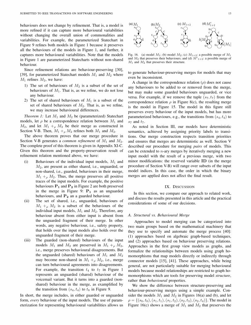
To compare the overall effectiveness of static matching,behavioural matching, and their combination, we computedtheir precision and recall for thresholds ranging from 0.95down to 0.5. The results are shown in Figure 14. As statedearlier in Section IV-C, threshold refers to the cutoff value usedfor determining the correspondence relation from the similaritydegrees.
In the studied models, states with typographically similarnames were likely to correspond. Hence, typographic match-ing, and by extension, static matching have high precision.However, static matching misses several correct matches,and hence has low recall. Behavioural matching, in contrast,has lower precision, but high recall. When the threshold isset reasonably high, combined matching has precision rateshigher than those of static and behavioural matching on theirown. This indicates that static and behavioural matching arefiltering out each other’s false positives. Recall remains high
SUBMITTED TO IEEE TRANSACTIONS ON SOFTWARE ENGINEERING 11
Fig. 12. Behavioural mapping between the models in Figure 1.
Fig. 13. Behavioural merge with respect to the relationship in Figure 12.
SUBMITTED TO IEEE TRANSACTIONS ON SOFTWARE ENGINEERING 12
Call Logger
0%
10%
20%
30%
40%
50%
60%
70%
80%
90%
100%
0.95 0.9 0.85 0.8 0.75 0.7 0.65 0.6 0.55 0.5
Threshold
Pre
cis
ion
Parallel Location
0%
10%
20%
30%
40%
50%
60%
70%
80%
90%
100%
0.95 0.9 0.85 0.8 0.75 0.7 0.65 0.6 0.55 0.5
Threshold
Pre
cis
ion
Remote Identification
0%
10%
20%
30%
40%
50%
60%
70%
80%
90%
100%
0.95 0.9 0.85 0.8 0.75 0.7 0.65 0.6 0.55 0.5
Threshold
Pre
cis
ion
Combined
Behavioural
Static
30%
40%
50%
60%
70%
80%
90%
100%
0.95 0.9 0.85 0.8 0.75 0.7 0.65 0.6 0.55 0.5
Threshold
Recall
30%
40%
50%
60%
70%
80%
90%
100%
0.95 0.9 0.85 0.8 0.75 0.7 0.65 0.6 0.55 0.5
Threshold
Recall
30%
40%
50%
60%
70%
80%
90%
100%
0.95 0.9 0.85 0.8 0.75 0.7 0.65 0.6 0.55 0.5
ThresholdRecall
Fig. 14. Results of static, behavioural, and combined matching.
TABLE IITRADEOFF POINTS BETWEEN PRECISION AND RECALL VALUES FOR THE
STUDIED VARIANT MODELS.
Feature Threshold Precision RecallCall Logger 0.80 54% 82%
Remote Identification 0.75 55% 100%Parallel Location 0.85 51% 81%
in the combined approach, as static matching and behaviouralmatching find many complimentary high-quality matches.
Table II shows the tradeoff points between precision andrecall values which we believe to be reasonable for our studiedvariant models. As shown in the table, for thresholds between0.75 and 0.85, our combined matcher achieved a precision ofmore than 50% and a recall of more than 80%. We anticipatethat for thresholds between 0.7 and 0.9, our technique wouldhave acceptable precision and recall; however, a more decisiveanswer to this question requires further evaluation.
VIII. PROPERTIES OF MERGE
Our approach to merge is useful if it produces semanticallycorrect results and scales well. Here, we discuss the complex-ity of our Merge operator and assess it by proving that itpreserves the behavioural properties of the input models.
A. Complexity of Merge
The space complexity of Merge is linear in the size of thecorrespondence relation ρ and the input models. Theoretically,the size of ρ is O(n1×n2). In practice, we expect the size of ρto be closer to max(n1, n2), giving us linear space complexityfor practical purposes. This was indeed the case for our models(see Table I). The time complexity of Merge is O(m1×m2).
B. Correctness of Merge
In this section, we prove that the merge procedure describedin Section V-B is behaviour-preserving (see Appendix XI-C fora detailed formal proof). The proof is based on showing that
the merge is related to each of the input models via behaviour-preserving refinement relations. Basing the notion of be-havioural merge on refinement relations is standard [12], [37].Such relations capture the process of combining behavioursof individual models while preserving all of their agreements.Our notion of merge and our behavioural formalisms, however,have some notable differences with the existing work [12],[37], summarized below.
Non-classical state machine formalisms have been previ-ously defined to capture partiality [38]. Such models havetwo types of transitions: for describing definite and partialbehaviours. In our work, in contrast, we use non-classicalstate machines to explicitly capture behavioural variabilities.Variant models differ on some of their behaviours, i.e., thosethat are non-shared, giving rise to variabilities. We use param-eterized Statecharts to explicitly differentiate between sharedbehaviours, i.e., those that are common between all variants,and non-shared behaviours, i.e., those that differ from onevariant to another. Specifically, in these Statechart models,transitions labelled by a condition on the reserved variableID represent the non-shared behaviours, and the rest of thetransitions – the shared ones.
Definition 2 (Parameterized Statecharts): A parameterizedStatechart M is a tuple (S, s, <h, E, V,Rshared , Rnonshared),where M shared = (S, s, <h, E, V,Rshared) is a Statechartrepresenting shared behaviours, i.e., containing the transi-tions not labelled with ID, and Mnonshared = (S, s, <h,E, V,Rnonshared) is a Statechart representing non-shared be-haviours, i.e., containing only the transitions with ID. Wedenote the set of both shared and non-shared transitions ofa parameterized Statechart by Rall = Rshared ∪ Rnonshared ,and we let Mall = (S, s, <h, E, V,Rall).
When a partial model evolves and goes through refinementsteps, the definite behaviours remain intact, but the partial be-haviours may turn into definite or prohibited behaviours [38].We define a new notion of refinement over parameterizedStatechart models where (1) the non-shared behaviours arepreserved through refinement, but the shared ones may turninto non-shared, and (2) the union of shared and non-shared
SUBMITTED TO IEEE TRANSACTIONS ON SOFTWARE ENGINEERING 13
behaviours does not change by refinement. That is, a model ismore refined if it can capture more behavioural variabilitieswithout changing the overall union of commonalities andvariabilities. For example, the parameterized Statechart inFigure 9 refines both models in Figure 1 because it preservesall the behaviours of the models in Figure 1, and further, itcaptures more behavioural variabilities. Note that the modelsin Figure 1 are parameterized Statecharts without non-sharedbehaviour.
Since refinement relations are behaviour-preserving [30],[39], for parameterized Statechart models M1 and M2 whereM1 refines M2, we have:
1) The set of behaviours of M2 is a subset of the set ofbehaviours of M1. That is, as we refine, we do not loseany behaviour.
2) The set of shared behaviours of M1 is a subset of theset of shared behaviours of M2. That is, as we refine,we may increase behavioural differences.
Theorem 1: Let M1 and M2 be (parameterized) Statechartmodels, let ρ be a correspondence relation between M1 andM2, and let M1 +ρ M2 be their merge as constructed inSection V-B. Then, M1 +ρM2 refines both M1 and M2.
The above theorem proves that our merge procedure inSection V-B generates a common refinement of M1 and M2.The complete proof of this theorem is given in Appendix XI-C.Given this theorem and the property-preservation result ofrefinement relation mentioned above, we have:
(i) Behaviours of the individual input models, M1 andM2, are present as either shared, i.e., unguarded, ornon-shared, i.e., guarded, behaviours in their merge,M1 +ρ M2. Thus, the merge preserves all positivetraces of the input models. For example, the positivebehaviours P1 and P2 in Figure 2 are both preservedin the merge in Figure 9: P1 as an unguardedbehaviours, and P2 an a guarded behaviour.
(ii) The set of shared, i.e., unguarded, behaviours ofM1 +ρ M2 is a subset of the behaviours of theindividual input models, M1 and M2. Therefore, anybehaviour absent from either input is absent fromthe unguarded fragment of their merge. In otherwords, any negative behaviour, i.e., safety property,that holds over the input models also holds over theunguarded fragment of their merge.
(iii) The guarded (non-shared) behaviours of the inputmodels M1 and M2 are preserved in M1 +ρ M2,i.e., merge preserves behavioural disagreements. Butthe unguarded (shared) behaviours of M1 and M2
may become non-shared in M1 +ρ M2, i.e., mergecan turn behavioural agreements into disagreements.For example, the transition t4 to t7 in Figure 1represents an unguarded (shared) behaviour of thevoicemail variant. But it turns into a guarded (non-shared) behaviour in the merge, as examplified bythe transition from (s4, t4) to t8 in Figure 9.
In short, the merge includes, in either guarded or unguardedform, every behaviour of the input models. The use of param-eterization for representing behavioural variabilities allows us
(a) (b) (c) (d)
c
a b
c c
a b
M1 M2 M1+2 M !1+2
s0
s1
s2
t0
t1 t2
t3 t4
c c
a ba[M1]
b[M1]
q0
q1q2
q3q4
r0
r1
r2
c
ba
Fig. 16. (a) model M1; (b) model M2; (c) M1+2: a possible merge of M1
and M2 that preserves their behaviours; and (d) M ′1+2: a possible merge ofM1 and M2 that preserves their structure.
to generate behaviour-preserving merges for models that mayeven be inconsistent.
A change in the correspondence relation (ρ) does not causeany behaviours to be added to or removed from the merge,but may make some guarded behaviours unguarded, or viceversa. For example, if we remove the tuple (s7, t7) from thecorrespondence relation ρ in Figure 8(c), the resulting mergeis the model in Figure 15. The model in this figure stillpreserves every behaviour of the input models, but has moreparameterized behaviours, e.g., the transitions from (s4, t4) tos7 and t7.
As noted in Section III, our models have deterministicsemantics, achieved by assigning priority labels to transi-tions. Our merge construction respects transition prioritiesand ensures that merges are deterministic as well. Section Vdescribed our procedure for merging pairs of models. Thiscan be extended to n-ary merges by iteratively merging a newinput model with the result of a previous merge, with twominor modifications: the reserved variable ID (in the mergeprocedure of Section V-B) will range over subsets of the inputmodel indices. In this case, the order in which the binarymerges are applied does not affect the final result.
IX. DISCUSSION
In this section, we compare our approach to related work,and discuss the results presented in this article and the practicalconsiderations of some of our decisions.
A. Structural vs. Behavioural Merge
Approaches to model merging can be categorized intotwo main groups based on the mathematical machinery thatthey use to specify and automate the merge process [40]:(1) approaches based on algebraic graph-based techniques,and (2) approaches based on behaviour preserving relations.Approaches in the first group view models as graphs, andformalize the relationships between models using graph ho-momorphisms that map models directly or indirectly throughconnector models [15], [41]. These approaches, while beinggeneral, are not particularly suitable for merging behaviouralmodels because model relationships are restricted to graph ho-momorphisms which are tools for preserving model structure,rather than behavioural properties.
We show the difference between structure-preserving andbehaviour-preserving merges using a simple example. Con-sider the models M1 and M2 in Figures 16(a) and (b), and letρ = {(s0, t0), (s1, t1), (s1, t2), (s2, t3), (s2, t4)}. The model inFigure 16(c) shows a merge of M1 and M2 that preserves the

SUBMITTED TO IEEE TRANSACTIONS ON SOFTWARE ENGINEERING 14
(Link Callee, Link Subscriber)
(Link Callee, Link Participant)
(Waiting, Pending)
(Timer Started, Timer Started)
Log Failure(Log Success, Log Success)
setup [zone =target]/callee = subscriber
setup [zone=source] /callee=participant
participant?Ack [ID=voicemail]
subscriber?Ack[ID=voicemail]
redirectToVoicemail[zone=target,ID=voicemail]
participant?Reject [zone=source, ID=basic] ORparticipant?TearDown [zone=source, ID=basic] OR
subscriber?Reject [zone=target, ID=basic] ORsubscriber?TearDown [zone=target, ID=basic]
participant?TearDown ORsubscriber?TearDown
participant?Accept [zone=source] ORsubscriber?Accept [zone=target]
Log Voicemail
(s0, t0)
callee?Ack[ID=basic]
callee?Ack[ ID=basic]
Call logger - (basic, voicemail)
(Start, Start)
Initialize Linkss1
(s2, t1)(s3, t2)
(s3, t3)
(s4, t4)
(s5, t5)
(s6, t6) t8
Log Failure
participant?Reject [zone=source, ID=voicemail] ORparticipant?Unavail [zone=source, ID=voicemail]OR
participant?TearDown [zone=source, ID=voicemail] ORsubscriber?Reject [zone=target, ID=voicemail] OR
subscriber?Unavail [in target-zone, ID=voicemail] ORsubscriber?TearDown [zone=target, ID=voicemail]
s7 t7
Fig. 15. The merge of the models in Figure 1 with respect to the relation in Figure 8(c) when (s7, t7) is removed from the relation.
structure of the input models: It is possible to embed eachof M1 and M2 into M1+2 using graph homomorphisms. Thismerge, however, does not preserve the behaviours of M1 andM2 because it collapses two behaviourally distinct states t1and t2 into a single state r1 in the merge. The model inFigure 16(d) is an alternative merge of M1 and M2 which isconstructed based on the notion of state machine refinementas proposed in this current article: It can be shown that M ′1+2
refines both M1 and M2. As shown in the figure, states t1 andt2 are respectively lifted to two distinct states, q1 and q2, inthis merge. By basing merge on refinement, we can chooseto keep states in the merged model distinct even if ρ mapsthem to one single state in the other model. The flexibility toduplicate states of the source models in the merge is essentialfor behaviour preservation but is not supported by the mergeapproaches that are based on graph homomorphisms.
B. Merging Models with Behavioural Discrepancies
Approaches to behavioural model merging generally spec-ify merge as a common behavioural refinement of the originalmodels. However, these approaches differ on how they handlediscrepancies between models both in their vocabulary andtheir behaviours. [42] shows that behavioural common refine-ments can be logically characterized as conjunction of theoriginal specifications when models are consistent and havethe same vocabulary. [13] introduces a notion of alphabet re-finement that allows to merge models with different vocabularybut consistent behaviours. The main focus of [13] is to usemerge as a way to elaborate partial models with unspecifiedvocabulary or unknown, but consistent, behaviours. Huth andPradhan [43] merge partial behavioural specifications wherea dominance ordering over models is given to resolve their
potential inconsistencies. These approaches do not providesupport for merging models with behavioural variabilities suchas those presented in Figure 1.
C. Analytical Reasoning for Matching Transition Labels
We have explored the use of analytical reasoning for com-paring transition labels. The N-gram algorithm, which is usedin this article for computing matching values for transitionlabels, is not suitable for comparing complex mathematicalexpressions. For example, it would find a rather small degreeof similarity between mathematical expressions (x ∧ y) ∨ zand (x∨ z)∧ (y ∨ z), whereas analytical reasoning, e.g., by atheorem prover, would identify these expressions as identical.While we did not encounter the need for such analysis on ourcase study, it might be necessary for such domains as webservices, where transition labels may include complex programsnippets.
D. Overlapping, Interacting and Cross-Cutting BehaviouralModels
Models which have been developed in a distributed mannermay relate to one another in a variety of ways. The nature ofthe relationships between such models depends primarily onthe intended application of the models and how they weredeveloped [44]. The work presented in this article focuseson merging a collection of inter-related models when rela-tionships describe overlaps between the models’ behaviours.Alternatively, relationships may describe shared interfacesfor interaction, in particular, when models are independentcomponents or features of a system, or the relationships maydescribe ways in which models alter one another’s behaviour(e.g., a cross-cutting model applied to other models) [45].
SUBMITTED TO IEEE TRANSACTIONS ON SOFTWARE ENGINEERING 15
The former kind of relationships is studied in the modelcomposition literature where the goal is to assemble a setof autonomous but interacting features that run sequentiallyor in parallel (e.g., [32], [46], [17], [30], [11]). Unlike merge,composition is concerned with how models communicate withone another through their interfaces rather than how theyoverlap in content. The latter relationships are studied in thearea of aspect-oriented development where the goal is to weavecross-cutting concerns into a base system (e.g., [47], [48],[49]). The focus of this article was on model merging and noton situations where model relationships describe interactionsor cross-cutting aspects.
E. Model Matching Techniques
Approaches to model matching can be exact or approx-imate. Exact matching is concerned with finding structuralor behavioural conformance relations between models. Graphhomomorphisms are examples of the former, whereas simu-lation and bisimulation relationships – of the latter. Findingexact correspondences between models has applications inmany fields including graph rewriting, pattern recognition,program analysis, and compiler optimization. However, itis not very useful for matching distributed models becausethe vocabularies and behaviours of these models seldom fittogether in an exact way, and thus, exact conformance relationsbetween these models are unlikely to be found.
Most domains use heuristic techniques for matching. Thesetechniques yield values denoting a likelihood of correspon-dence between elements of different models. In databasedesign, finding correspondences between database schemata isreferred to as schema matching [50]. State-of-the-art schemamatchers, such as Protoplasm [9], combine several heuristicsfor computing similarities between schema elements. Ourtypographic and linguistic heuristics (Section IV-A) are verysimilar to those used in schema matching, but our otherheuristics are tailored to behavioural models.
Several approaches to matching have been proposed insoftware engineering. Maiden and Sutcliffe [6] employ heuris-tic reasoning for finding analogies between a problem de-scription and already existing domain abstractions. Ryan andMathews [51] use approximate graph matching for findingoverlaps between concept graphs. Alspaugh et. al. [52] pro-pose term matching based on project glossaries for findingsimilarities between textual scenarios. Mandelin et. al. [4]combine diagrammatic and syntactic heuristics for findingmatches between architecture models. Xing and Stroulia [53]use heuristic-based name-similarity and structure-similaritymatchers to identify conceptually similar entities in UMLclass diagrams. None of these approaches were specificallydesigned for behavioural models and are either inapplicableor unsuitable for matching Statechart models.
Some matching approaches deal with behavioural mod-els of a different kind. For example, Kelter and Schmidt[54] discuss differencing mechanisms specifically designedfor UML Statecharts. This work assumes that models aredeveloped centrally within a unified modelling environment.Other approaches apply to independently-developed models.
Lohmann [55] and Zisman et. al. [8] define similarity measuresbetween web-services to identify candidate services to replacea service in use when it becomes unavailable or unsuitabledue to a change. Quante and Koschke [56] propose similaritymeasures between finite state automata generated by differentreverse engineering mechanisms to compare the effectivenessof these mechanisms. Bogdanov and Walkinshaw [57] providean algorithm for comparing LTSs without relying on the initialstate or any particular states of the underlying models as thereference point. None of these are applicable both to ourparticular purpose (comparing different versions of the samefeature), and to our particular class of models (Statechartsmodels). Further, the evaluation of our matching technique istargeted at behavioural models built in the telecommunicationdomain. To our knowledge, the usefulness and effectiveness ofmodel matching have not been studied in this context before.
In computer science theory, several notions of behaviouralconformance have been proposed to capture the behaviouralsimilarity between models with quantitative features such astime or probability [58]. For these models, a discrete notion ofsimilarity, i.e., models are either equivalent or they are not, isnot helpful because minor changes in the quantitative data maycause equivalent models to become inequivalent, even if thedifference between their behaviours is very minor. Therefore,instead of equivalences that result in a binary answer, oneneeds to use relations that can differentiate between slightlydifferent and completely different models. Examples of suchrelations are stochastic or Markovian notions of behaviouralsimilarity (e.g., [59], [60]). Our formulation of behaviouralsimilarity (Section IV-B) is analogous to these similarityrelations. The goal of this work is to define a distance metricover the space of (quantitative) reactive processes and studythe mathematical properties of the metric. Our goal, instead,is to obtain a similarity measure that can detect pairs of stateswith a high degree of behavioural similarity.
F. Model Merging Techniques
Model merging spans several application areas. In databasedesign, merge is an important step for producing a schemacapturing the data requirements of all the stakeholders [2].Software engineering deals extensively with model merging –several papers study the subject in specific domains, includingearly requirements [15], static UML diagrams [61], [14],[62], [63], [64], and declarative specifications [65]. None ofthese were specifically designed for behavioural models andare either inapplicable or unsuitable for matching Statechartmodels. We compared our work with existing approaches formerging behavioural models in Section IX-B.
There has also been work on defining languages for modelmerging, e.g., the Epsilon Merging Language (EML) [10] andAtlas Model Management Architecture (AMMA) [66]. EMLis a rule-based language for merging models with the same ordifferent meta-models. The language distinguishes four phasesin the merge process and provides flexible constructs fordefining the rules that should be applied in each phase. AMMAfacilitates modelling tasks such as merging using model trans-formation languages defined between different meta-models.
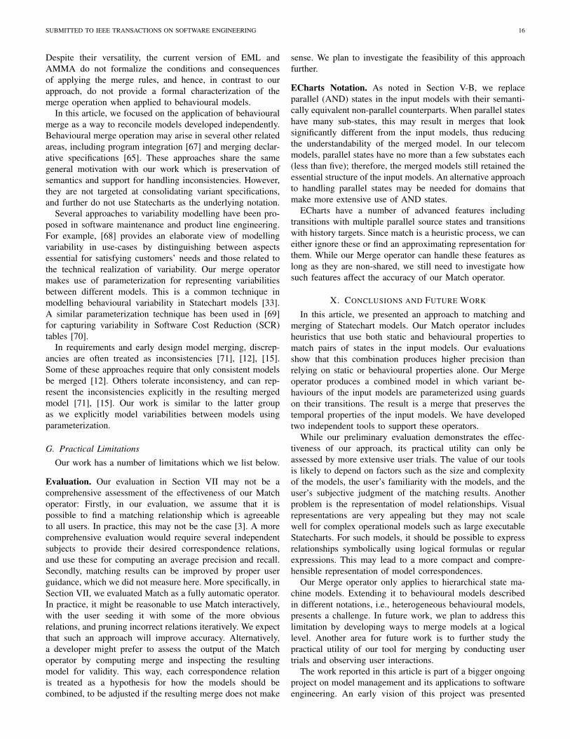
SUBMITTED TO IEEE TRANSACTIONS ON SOFTWARE ENGINEERING 16
Despite their versatility, the current version of EML andAMMA do not formalize the conditions and consequencesof applying the merge rules, and hence, in contrast to ourapproach, do not provide a formal characterization of themerge operation when applied to behavioural models.
In this article, we focused on the application of behaviouralmerge as a way to reconcile models developed independently.Behavioural merge operation may arise in several other relatedareas, including program integration [67] and merging declar-ative specifications [65]. These approaches share the samegeneral motivation with our work which is preservation ofsemantics and support for handling inconsistencies. However,they are not targeted at consolidating variant specifications,and further do not use Statecharts as the underlying notation.
Several approaches to variability modelling have been pro-posed in software maintenance and product line engineering.For example, [68] provides an elaborate view of modellingvariability in use-cases by distinguishing between aspectsessential for satisfying customers’ needs and those related tothe technical realization of variability. Our merge operatormakes use of parameterization for representing variabilitiesbetween different models. This is a common technique inmodelling behavioural variability in Statechart models [33].A similar parameterization technique has been used in [69]for capturing variability in Software Cost Reduction (SCR)tables [70].
In requirements and early design model merging, discrep-ancies are often treated as inconsistencies [71], [12], [15].Some of these approaches require that only consistent modelsbe merged [12]. Others tolerate inconsistency, and can rep-resent the inconsistencies explicitly in the resulting mergedmodel [71], [15]. Our work is similar to the latter groupas we explicitly model variabilities between models usingparameterization.
G. Practical Limitations
Our work has a number of limitations which we list below.
Evaluation. Our evaluation in Section VII may not be acomprehensive assessment of the effectiveness of our Matchoperator: Firstly, in our evaluation, we assume that it ispossible to find a matching relationship which is agreeableto all users. In practice, this may not be the case [3]. A morecomprehensive evaluation would require several independentsubjects to provide their desired correspondence relations,and use these for computing an average precision and recall.Secondly, matching results can be improved by proper userguidance, which we did not measure here. More specifically, inSection VII, we evaluated Match as a fully automatic operator.In practice, it might be reasonable to use Match interactively,with the user seeding it with some of the more obviousrelations, and pruning incorrect relations iteratively. We expectthat such an approach will improve accuracy. Alternatively,a developer might prefer to assess the output of the Matchoperator by computing merge and inspecting the resultingmodel for validity. This way, each correspondence relationis treated as a hypothesis for how the models should becombined, to be adjusted if the resulting merge does not make
sense. We plan to investigate the feasibility of this approachfurther.
ECharts Notation. As noted in Section V-B, we replaceparallel (AND) states in the input models with their semanti-cally equivalent non-parallel counterparts. When parallel stateshave many sub-states, this may result in merges that looksignificantly different from the input models, thus reducingthe understandability of the merged model. In our telecommodels, parallel states have no more than a few substates each(less than five); therefore, the merged models still retained theessential structure of the input models. An alternative approachto handling parallel states may be needed for domains thatmake more extensive use of AND states.
ECharts have a number of advanced features includingtransitions with multiple parallel source states and transitionswith history targets. Since match is a heuristic process, we caneither ignore these or find an approximating representation forthem. While our Merge operator can handle these features aslong as they are non-shared, we still need to investigate howsuch features affect the accuracy of our Match operator.
X. CONCLUSIONS AND FUTURE WORK
In this article, we presented an approach to matching andmerging of Statechart models. Our Match operator includesheuristics that use both static and behavioural properties tomatch pairs of states in the input models. Our evaluationsshow that this combination produces higher precision thanrelying on static or behavioural properties alone. Our Mergeoperator produces a combined model in which variant be-haviours of the input models are parameterized using guardson their transitions. The result is a merge that preserves thetemporal properties of the input models. We have developedtwo independent tools to support these operators.
While our preliminary evaluation demonstrates the effec-tiveness of our approach, its practical utility can only beassessed by more extensive user trials. The value of our toolsis likely to depend on factors such as the size and complexityof the models, the user’s familiarity with the models, and theuser’s subjective judgment of the matching results. Anotherproblem is the representation of model relationships. Visualrepresentations are very appealing but they may not scalewell for complex operational models such as large executableStatecharts. For such models, it should be possible to expressrelationships symbolically using logical formulas or regularexpressions. This may lead to a more compact and compre-hensible representation of model correspondences.
Our Merge operator only applies to hierarchical state ma-chine models. Extending it to behavioural models describedin different notations, i.e., heterogeneous behavioural models,presents a challenge. In future work, we plan to address thislimitation by developing ways to merge models at a logicallevel. Another area for future work is to further study thepractical utility of our tool for merging by conducting usertrials and observing user interactions.
The work reported in this article is part of a bigger ongoingproject on model management and its applications to softwareengineering. An early vision of this project was presented
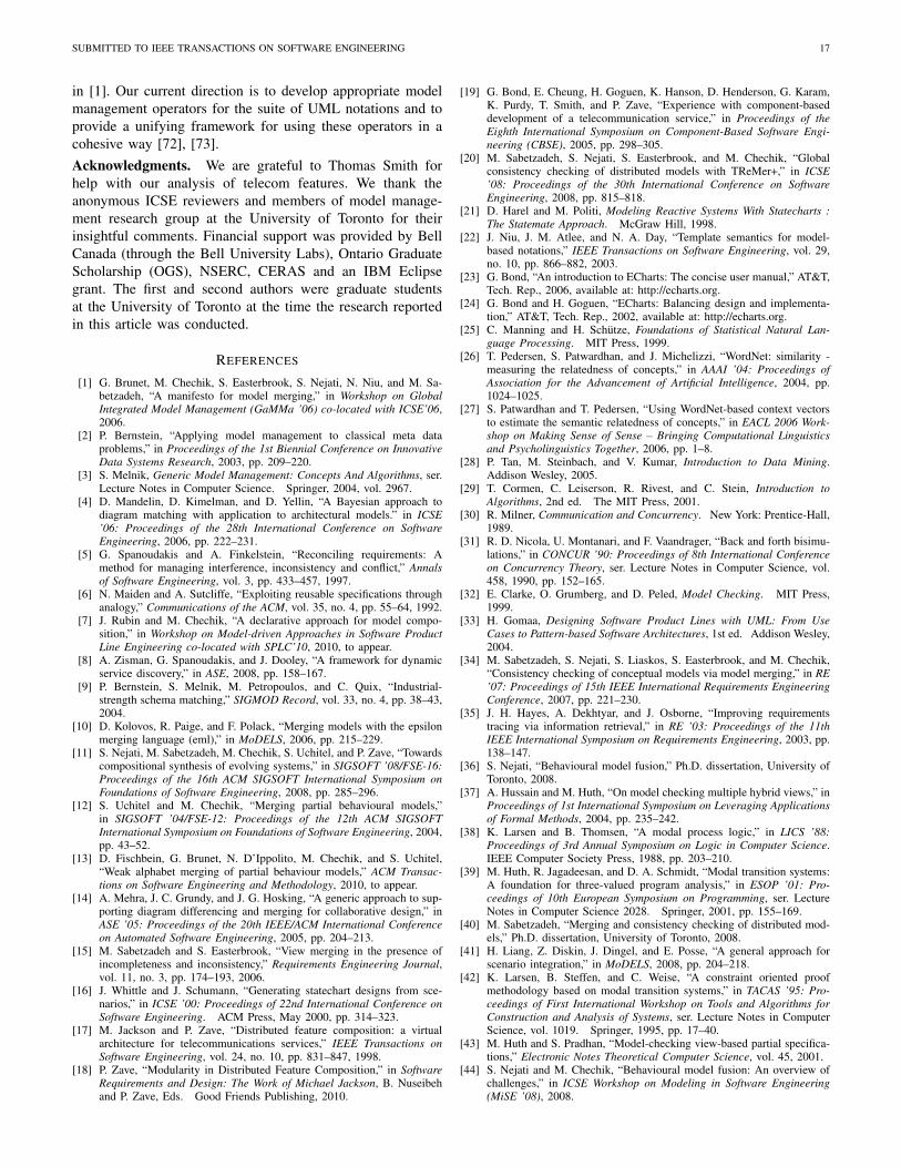
SUBMITTED TO IEEE TRANSACTIONS ON SOFTWARE ENGINEERING 17
in [1]. Our current direction is to develop appropriate modelmanagement operators for the suite of UML notations and toprovide a unifying framework for using these operators in acohesive way [72], [73].Acknowledgments. We are grateful to Thomas Smith forhelp with our analysis of telecom features. We thank theanonymous ICSE reviewers and members of model manage-ment research group at the University of Toronto for theirinsightful comments. Financial support was provided by BellCanada (through the Bell University Labs), Ontario GraduateScholarship (OGS), NSERC, CERAS and an IBM Eclipsegrant. The first and second authors were graduate studentsat the University of Toronto at the time the research reportedin this article was conducted.
REFERENCES
[1] G. Brunet, M. Chechik, S. Easterbrook, S. Nejati, N. Niu, and M. Sa-betzadeh, “A manifesto for model merging,” in Workshop on GlobalIntegrated Model Management (GaMMa ’06) co-located with ICSE’06,2006.
[2] P. Bernstein, “Applying model management to classical meta dataproblems,” in Proceedings of the 1st Biennial Conference on InnovativeData Systems Research, 2003, pp. 209–220.
[3] S. Melnik, Generic Model Management: Concepts And Algorithms, ser.Lecture Notes in Computer Science. Springer, 2004, vol. 2967.
[4] D. Mandelin, D. Kimelman, and D. Yellin, “A Bayesian approach todiagram matching with application to architectural models.” in ICSE’06: Proceedings of the 28th International Conference on SoftwareEngineering, 2006, pp. 222–231.
[5] G. Spanoudakis and A. Finkelstein, “Reconciling requirements: Amethod for managing interference, inconsistency and conflict,” Annalsof Software Engineering, vol. 3, pp. 433–457, 1997.
[6] N. Maiden and A. Sutcliffe, “Exploiting reusable specifications throughanalogy,” Communications of the ACM, vol. 35, no. 4, pp. 55–64, 1992.
[7] J. Rubin and M. Chechik, “A declarative approach for model compo-sition,” in Workshop on Model-driven Approaches in Software ProductLine Engineering co-located with SPLC’10, 2010, to appear.
[8] A. Zisman, G. Spanoudakis, and J. Dooley, “A framework for dynamicservice discovery,” in ASE, 2008, pp. 158–167.
[9] P. Bernstein, S. Melnik, M. Petropoulos, and C. Quix, “Industrial-strength schema matching,” SIGMOD Record, vol. 33, no. 4, pp. 38–43,2004.
[10] D. Kolovos, R. Paige, and F. Polack, “Merging models with the epsilonmerging language (eml),” in MoDELS, 2006, pp. 215–229.
[11] S. Nejati, M. Sabetzadeh, M. Chechik, S. Uchitel, and P. Zave, “Towardscompositional synthesis of evolving systems,” in SIGSOFT ’08/FSE-16:Proceedings of the 16th ACM SIGSOFT International Symposium onFoundations of Software Engineering, 2008, pp. 285–296.
[12] S. Uchitel and M. Chechik, “Merging partial behavioural models,”in SIGSOFT ’04/FSE-12: Proceedings of the 12th ACM SIGSOFTInternational Symposium on Foundations of Software Engineering, 2004,pp. 43–52.
[13] D. Fischbein, G. Brunet, N. D’Ippolito, M. Chechik, and S. Uchitel,“Weak alphabet merging of partial behaviour models,” ACM Transac-tions on Software Engineering and Methodology, 2010, to appear.
[14] A. Mehra, J. C. Grundy, and J. G. Hosking, “A generic approach to sup-porting diagram differencing and merging for collaborative design,” inASE ’05: Proceedings of the 20th IEEE/ACM International Conferenceon Automated Software Engineering, 2005, pp. 204–213.
[15] M. Sabetzadeh and S. Easterbrook, “View merging in the presence ofincompleteness and inconsistency,” Requirements Engineering Journal,vol. 11, no. 3, pp. 174–193, 2006.
[16] J. Whittle and J. Schumann, “Generating statechart designs from sce-narios,” in ICSE ’00: Proceedings of 22nd International Conference onSoftware Engineering. ACM Press, May 2000, pp. 314–323.
[17] M. Jackson and P. Zave, “Distributed feature composition: a virtualarchitecture for telecommunications services,” IEEE Transactions onSoftware Engineering, vol. 24, no. 10, pp. 831–847, 1998.
[18] P. Zave, “Modularity in Distributed Feature Composition,” in SoftwareRequirements and Design: The Work of Michael Jackson, B. Nuseibehand P. Zave, Eds. Good Friends Publishing, 2010.
[19] G. Bond, E. Cheung, H. Goguen, K. Hanson, D. Henderson, G. Karam,K. Purdy, T. Smith, and P. Zave, “Experience with component-baseddevelopment of a telecommunication service,” in Proceedings of theEighth International Symposium on Component-Based Software Engi-neering (CBSE), 2005, pp. 298–305.
[20] M. Sabetzadeh, S. Nejati, S. Easterbrook, and M. Chechik, “Globalconsistency checking of distributed models with TReMer+,” in ICSE’08: Proceedings of the 30th International Conference on SoftwareEngineering, 2008, pp. 815–818.
[21] D. Harel and M. Politi, Modeling Reactive Systems With Statecharts :The Statemate Approach. McGraw Hill, 1998.
[22] J. Niu, J. M. Atlee, and N. A. Day, “Template semantics for model-based notations,” IEEE Transactions on Software Engineering, vol. 29,no. 10, pp. 866–882, 2003.
[23] G. Bond, “An introduction to ECharts: The concise user manual,” AT&T,Tech. Rep., 2006, available at: http://echarts.org.
[24] G. Bond and H. Goguen, “ECharts: Balancing design and implementa-tion,” AT&T, Tech. Rep., 2002, available at: http://echarts.org.
[25] C. Manning and H. Schutze, Foundations of Statistical Natural Lan-guage Processing. MIT Press, 1999.
[26] T. Pedersen, S. Patwardhan, and J. Michelizzi, “WordNet: similarity -measuring the relatedness of concepts,” in AAAI ’04: Proceedings ofAssociation for the Advancement of Artificial Intelligence, 2004, pp.1024–1025.
[27] S. Patwardhan and T. Pedersen, “Using WordNet-based context vectorsto estimate the semantic relatedness of concepts,” in EACL 2006 Work-shop on Making Sense of Sense – Bringing Computational Linguisticsand Psycholinguistics Together, 2006, pp. 1–8.
[28] P. Tan, M. Steinbach, and V. Kumar, Introduction to Data Mining.Addison Wesley, 2005.
[29] T. Cormen, C. Leiserson, R. Rivest, and C. Stein, Introduction toAlgorithms, 2nd ed. The MIT Press, 2001.
[30] R. Milner, Communication and Concurrency. New York: Prentice-Hall,1989.
[31] R. D. Nicola, U. Montanari, and F. Vaandrager, “Back and forth bisimu-lations,” in CONCUR ’90: Proceedings of 8th International Conferenceon Concurrency Theory, ser. Lecture Notes in Computer Science, vol.458, 1990, pp. 152–165.
[32] E. Clarke, O. Grumberg, and D. Peled, Model Checking. MIT Press,1999.
[33] H. Gomaa, Designing Software Product Lines with UML: From UseCases to Pattern-based Software Architectures, 1st ed. Addison Wesley,2004.
[34] M. Sabetzadeh, S. Nejati, S. Liaskos, S. Easterbrook, and M. Chechik,“Consistency checking of conceptual models via model merging,” in RE’07: Proceedings of 15th IEEE International Requirements EngineeringConference, 2007, pp. 221–230.
[35] J. H. Hayes, A. Dekhtyar, and J. Osborne, “Improving requirementstracing via information retrieval,” in RE ’03: Proceedings of the 11thIEEE International Symposium on Requirements Engineering, 2003, pp.138–147.
[36] S. Nejati, “Behavioural model fusion,” Ph.D. dissertation, University ofToronto, 2008.
[37] A. Hussain and M. Huth, “On model checking multiple hybrid views,” inProceedings of 1st International Symposium on Leveraging Applicationsof Formal Methods, 2004, pp. 235–242.
[38] K. Larsen and B. Thomsen, “A modal process logic,” in LICS ’88:Proceedings of 3rd Annual Symposium on Logic in Computer Science.IEEE Computer Society Press, 1988, pp. 203–210.
[39] M. Huth, R. Jagadeesan, and D. A. Schmidt, “Modal transition systems:A foundation for three-valued program analysis,” in ESOP ’01: Pro-ceedings of 10th European Symposium on Programming, ser. LectureNotes in Computer Science 2028. Springer, 2001, pp. 155–169.
[40] M. Sabetzadeh, “Merging and consistency checking of distributed mod-els,” Ph.D. dissertation, University of Toronto, 2008.
[41] H. Liang, Z. Diskin, J. Dingel, and E. Posse, “A general approach forscenario integration,” in MoDELS, 2008, pp. 204–218.
[42] K. Larsen, B. Steffen, and C. Weise, “A constraint oriented proofmethodology based on modal transition systems,” in TACAS ’95: Pro-ceedings of First International Workshop on Tools and Algorithms forConstruction and Analysis of Systems, ser. Lecture Notes in ComputerScience, vol. 1019. Springer, 1995, pp. 17–40.
[43] M. Huth and S. Pradhan, “Model-checking view-based partial specifica-tions,” Electronic Notes Theoretical Computer Science, vol. 45, 2001.
[44] S. Nejati and M. Chechik, “Behavioural model fusion: An overview ofchallenges,” in ICSE Workshop on Modeling in Software Engineering(MiSE ’08), 2008.
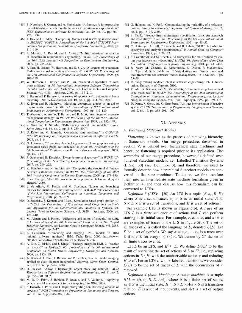
SUBMITTED TO IEEE TRANSACTIONS ON SOFTWARE ENGINEERING 18
[45] B. Nuseibeh, J. Kramer, and A. Finkelstein, “A framework for expressingthe relationships between multiple views in requirements specification,”IEEE Transaction on Software Engineering, vol. 20, no. 10, pp. 760–773, 1994.
[46] J. Hay and J. Atlee, “Composing features and resolving interactions,”in SIGSOFT ’00/FSE-8: Proceedings of the 8th ACM SIGSOFT Inter-national Symposium on Foundations of Software Engineering, 2000, pp.110–119.
[47] A. Moreira, A. Rashid, and J. Araujo, “Multi-dimensional separationof concerns in requirements engineering,” in RE ’05: Proceedings ofthe 10th IEEE International Symposium on Requirements Engineering,2005, pp. 285–296.
[48] P. Tarr, H. Ossher, W. Harrison, and S. S. Jr., “N degrees of separation:Multi-dimensional separation of concerns,” in ICSE ’99: Proceedings ofthe 21st International Conference on Software Engineering, 1999, pp.107–119.
[49] W. Harrison, H. Ossher, and P. Tarr, “General composition of soft-ware artifacts,” in 5th International Symposium Software Composition(SC’06), co-located with ETAPS’06, ser. Lecture Notes in ComputerScience, vol. 4089. Springer, 2006, pp. 194–210.
[50] E. Rahm and P. Bernstein, “A survey of approaches to automatic schemamatching,” The VLDB Journal, vol. 10, no. 4, pp. 334–350, 2001.
[51] K. Ryan and B. Mathews, “Matching conceptual graphs as an aid torequirements re-use,” in RE ’93: Proceedings of IEEE InternationalSymposium on Requirements Engineering, 1993, pp. 112–120.
[52] T. Alspaugh, A. Anton, T. Barnes, and B. Mott, “An integrated scenariomanagement strategy,” in RE ’99: Proceedings of the 4th IEEE Interna-tional Symposium on Requirements Engineering, 1999, pp. 142–149.
[53] Z. Xing and E. Stroulia, “Differencing logical uml models,” Autom.Softw. Eng., vol. 14, no. 2, pp. 215–259, 2007.
[54] U. Kelter and M. Schmidt, “Comparing state machines,” in CVSM’08:ICSE’08 Workshop on Comparison and versioning of software models,2008, pp. 1–6.
[55] N. Lohmann, “Correcting deadlocking service choreographies using asimulation-based graph edit distance,” in BPM ’08: Proceedings of the6th International Conference on Business Process Management, 2008,pp. 132–147.
[56] J. Quante and R. Koschke, “Dynamic protocol recovery,” in WCRE ’07:Proceedings of the 14th Working Conference on Reverse Engineering,2007, pp. 219–228.
[57] K. Bogdanov and N. Walkinshaw, “Computing the structural differencebetween state-based models,” in WCRE ’09: Proceedings of the 200916th Working Conference on Reverse Engineering, 2009, pp. 177–186.
[58] F. van Breugel, “Abe ’08: Workshop on approximate behavioural equiv-alences,” 2008.
[59] L. de Alfaro, M. Faella, and M. Stoelinga, “Linear and branchingmetrics for quantitative transition systems,” in ICALP ’04: Proceedingsof the 31st International Colloquium on Automata, Languages andProgramming, 2004, pp. 97–109.
[60] O. Sokolsky, S. Kannan, and I. Lee, “Simulation-based graph similarity,”in TACAS ’06: Proceedings of 12th International Conference on Toolsand Algorithms for the Construction and Analysis of Systems, ser.Lecture Notes in Computer Science, vol. 3920. Springer, 2006, pp.426–440.
[61] M. Alanen and I. Porres, “Difference and union of models,” in UML’03: Proceedings of the 6th International Conference on The UnifiedModeling Language, ser. Lecture Notes in Computer Science, vol. 2863.Springer, 2003, pp. 2–17.
[62] K. Letkeman, “Comparing and merging UML models in IBMrational software architect,” IBM, Tech. Rep., 2006, http://www-306.ibm.com/software/awdtools/architect/swarchitect/.
[63] A. Zito, Z. Diskin, and J. Dingel, “Package merge in UML 2: Practicevs. theory?” in MoDELS ’06: Proceedings of the 9th InternationalConference on Model Driven Engineering Languages and Systems,2006, pp. 185–199.
[64] A. Boronat, J. Carsı, I. Ramos, and P. Letelier, “Formal model mergingapplied to class diagram integration,” Electron. Notes Theor. Comput.Sci., vol. 166, pp. 5–26, 2007.
[65] D. Jackson, “Alloy: a lightweight object modelling notation,” ACMTransactions on Software Engineering and Methodology, vol. 11, no. 2,pp. 256–290, 2002.
[66] M. D. D. Fabro, J. Bezivin, F. Jouault, and P. Valduriez, “Applyinggeneric model management to data mapping,” in BDA, 2005.
[67] S. Horwitz, J. Prins, and T. Reps, “Integrating noninterfering versions ofprograms,” ACM Transaction on Programming Languages and Systems,vol. 11, no. 3, pp. 345–387, 1989.
[68] G. Halmans and K. Pohl, “Communicating the variability of a software-product family to customers,” Software and System Modeling, vol. 2,no. 1, pp. 15–36, 2003.
[69] S. Faulk, “Product-line requirements specification (prs): An approachand case study,” in RE ’01: Proceedings of the 6th IEEE InternationalSymposium on Requirements Engineering, 2001, pp. 48–55.
[70] C. Heitmeyer, A. Bull, C. Gasarch, and B. Labaw, “SCR*: A toolset forspecifying and analyzing requirements,” in Annual Conf. on ComputerAssurance, 1995, pp. 109–122.
[71] S. Easterbrook and M. Chechik, “A framework for multi-valued reason-ing over inconsistent viewpoints,” in ICSE ’01: Proceedings of the 23rdInternational Conference on Software Engineering, 2001, pp. 411–420.
[72] R. Salay, M. Chechik, S. Easterbrook, Z. Diskin, P. McCormick,S. Nejati, M. Sabetzadeh, and P. Viriyakattiyaporn, “An eclipse-basedtool framework for software model management,” in ETX, 2007, pp.55–59.
[73] R. Salay, “Using modeler intent in software engineering,” Ph.D. disser-tation, University of Toronto, 2010.
[74] R. Alur, S. Kannan, and M. Yannakakis, “Communicating hierarchicalstate machines,” in ICALP ’99: Proceedings of the 26th InternationalColloquium on Automata, Languages and Programming, ser. LectureNotes in Computer Science, vol. 1644. Springer, 1999, pp. 169–178.
[75] D. Dams, R. Gerth, and O. Grumberg, “Abstract interpretation of reactivesystems,” ACM Transactions on Programming Languages and Systems,vol. 2, no. 19, pp. 253–291, 1997.
XI. APPENDIX
A. Flattening Statechart Models
Flattening is known as the process of removing hierarchyin Statechart models. Our merge procedure, described inSection V, is defined over hierarchical state machines, andhence, no flattening is required prior to its application. Thesemantics of our merge procedure, however, is defined overflattened Statechart models, i.e., Labelled Transition Systems(LTSs) [30] (see Definition 3), and therefore, we need toformally describe how hierarchical Statechart models are con-verted to flat state machines. To do so, we first translatethem into an intermediate state machine formalism given inDefinition 4, and then discuss how this formalism can beconverted to LTSs.
Definition 3 (LTS): [30] An LTS is a tuple (S, s0, R,E)where S is a set of states, s0 ∈ S is an initial state, R ⊆S × E × S is a set of transitions, and E is a set of actions.
An example LTS is shown in Figure 5(b). A trace of anLTS L is a finite sequence σ of actions that L can performstarting at its initial state. For example, ε, a, a · c, and a · c · care examples of traces of the LTS in Figure 5(b). The set ofall traces of L is called the language of L, denoted L(L). LetΣ be a set of symbols. We say σ = e0e1 . . . en is a trace overΣ if ei ∈ Σ for every 0 ≤ i ≤ n. We denote by Σ∗ the set ofall finite traces over Σ.
Let L be an LTS, and E′ ⊆ E. We define L@E′ to be theresult of restricting the set of actions of L to E′, i.e., replacingactions in E \E′ with the unobservable action τ and reducingE to E′. For an LTS L with τ -labelled transitions, we considerL(L) to be the set of traces of L with the occurrences of τremoved.
Definition 4 (State Machine): A state machine is a tupleSM = (S, s0, R,E,Act), where S is a finite set of states,s0 ∈ S is the initial state, R ⊆ S×E×Act×S is a transitionrelation, E is a set of input events, and Act is a set of outputactions.
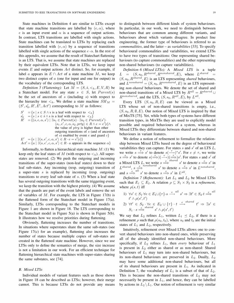
SUBMITTED TO IEEE TRANSACTIONS ON SOFTWARE ENGINEERING 19
State machines in Definition 4 are similar to LTSs exceptthat state machine transitions are labelled by (e, α), wheree is an input event and α is a sequence of output actions.In contrast, LTS transitions are labelled with single actions.State machines can be translated to LTSs by replacing eachtransition labelled with (e, α) by a sequence of transitionslabelled with single actions of the sequence e ·α. In the rest ofthis appendix, we assume that the result of Statechart flatteningis an LTS. That is, we assume that state machines are replacedby their equivalent LTSs. Note that in LTSs, we keep inputevents E and output actions Act distinct. So, for example, iflabel a appears in E ∩ Act of a state machine M , we keeptwo distinct copies of a (one for input and one for output) inthe vocabulary of the corresponding LTS.
Definition 5 (Flattening): Let M = (S, s, <h, E, V,R) bea Statechart model. For any state s ∈ S, let Parent(s)be the set of ancestors of s (including s) with respect tothe hierarchy tree <h. We define a state machine SMM =(S′, s′0, R
′, E′,Act ′) corresponding to M as follows:
S′ = {s | s ∈ S ∧ s is a leaf with respect to <h}s′0 = {s | s ∈ s ∧ s is a leaf with respect to <h}R′ = {(s, e, α, s′) | ∃s1 ∈ Parent(s) · ∃s2 ∈ Parent(s′)·
〈s1, e′, c, α, s2, prty〉 ∈ R ∧ e = e′[c]∧the value of ptry is higher than otheroutgoing transitions of s (and of ancestorsof s) enabled by event e and guard c}
E′ = {e | ∃〈s, e′, c, α, s′〉 ∈ R · e = e′[c]}Act ′= {a | ∃〈s, e′, c, α, s′〉 ∈ R · a appears in the sequence α}
Informally, to flatten a hierarchical state machine M : (1) Wekeep only the leaf states of M (with respect to <h). All super-states are removed. (2) We push the outgoing and incomingtransitions of the super-states (non-leaf states) down to theirleaf sub-states. Any incoming (resp. outgoing) transition ofa super-state s is replaced by incoming (resp. outgoing)transitions to every leaf sub-state of s. (3) When a leaf statehas several outgoing transitions with the same triggering event,we keep the transition with the highest priority. (4) We assumethat the guards are part of the event labels and remove the setof variables of M . For example, the LTS in Figure 17(b) isthe flattened form of the Statechart model in Figure 17(a).Similarly, LTSs corresponding to the Statechart models inFigure 1 are shown in Figure 18. The LTS corresponding tothe Statechart model in Figure 5(a) is shown in Figure 5(b).It illustrates how we resolve priorities during flattening.
Obviously, flattening increases the number of transitions.In situations where superstates share the same sub-states (seeFigure 17(c) for an example), flattening also increases thenumber of states because multiple copies of sub-states arecreated in the flattened state machine. However, since we useLTSs only to define the semantics of merge, the size increaseis not a limitation in our work. For an efficient technique forflattening hierarchical state machines with super-states sharingthe same substates, see [74].
B. Mixed LTSs
Individual models of variant features such as those shownin Figure 18 can be described as LTSs; however, their mergecannot. This is because LTSs do not provide any means
to distinguish between different kinds of system behaviours.In particular, in our work, we need to distinguish betweenbehaviours that are common among different variants, andbehaviours about which variants disagree. In product lineengineering, the former type of behaviours is referred to ascommonalities, and the latter – as variabilities [33]. To specifybehavioural commonalities and variabilities, we extend LTSsto have two types of transitions: One representing shared be-haviours (to capture commonalities) and the other representingnon-shared behaviours (to capture variabilities).
Definition 6 (Mixed LTSs): A Mixed LTS is a tupleL = (S, s0, Rshared , Rnonshared , E), where Lshared =(S, s0, Rshared , E) is an LTS representing shared behaviours,and Lnonshared = (S, s0, Rnonshared , E) is an LTS represent-ing non-shared behaviours. We denote the set of shared andnon-shared transitions of a Mixed LTS by Rall = Rshared ∪Rnonshared, and the LTS, (S, s0, Rall , E), by Lall .
Every LTS (S, s0, R,E) can be viewed as a MixedLTS whose set of non-shared transitions is empty, i.e.,(S, s0, R, ∅, E). Our notion of Mixed LTS is inspired by thatof MixTS [75]. Yet, while both types of systems have differenttransition types, in MixTSs they are used to explicitly modelpossible and required behaviours of a system, whereas inMixed LTSs they differentiate between shared and non-sharedbehaviours in variant features.
We define a notion of refinement to formalize the relation-ship between Mixed LTSs based on the degree of behaviouralvariabilities they can capture. For states s and s′ of an LTS L,we write s τ=⇒ s′ to denote s( τ−→)∗s′. For e 6= τ , we writes
e=⇒ s′ to denote s( τ=⇒)( e−→)( τ=⇒)s′. For states s and s′ ofa Mixed LTS L, we write s e=⇒shared
s′ to denote s e=⇒ s′ inLshared , s e=⇒nonshared
s′ to denote s e=⇒ s′ in Lnonshared ,and s e=⇒all
s′ to denote s e=⇒ s′ in Lall .Definition 7 (Refinement): Let L1 and L2 be Mixed LTSs
such that E1 ⊆ E2 . A relation ρ ⊆ S1 × S2 is a refinement,where ρ(s, t) iff
1) ∀s′ ∈ S1·∀e ∈ E1∪{τ}·s e−→alls′ ⇒ ∃t′ ∈ S2·t e=⇒all
t′ ∧ ρ(s′, t′)2) ∀t′ ∈ S2 · ∀e ∈ E2 ∪ {τ} · t e−→shared
t′ ⇒ ∃s′ ∈S1 · s e=⇒shared
s′ ∧ ρ(s′, t′)
We say that L2 refines L1, written L1 � L2, if there is arefinement ρ such that ρ(s0, t0), where s0 and t0 are the initialstates of L1 and L2, respectively.
Intuitively, refinement over Mixed LTSs allows one to con-vert shared behaviours into non-shared ones, while preservingall of the already identified non-shared behaviours. Morespecifically, if L2 refines L1, then every behaviour of L1
is present in L2 either as shared or as non-shared: Sharedbehaviours of L1 may turn into non-shared behaviours, butits non-shared behaviours are preserved in L2. Dually, L2
may have some additional non-shared behaviours, but allof its shared behaviours are present in L1. As indicated inDefinition 7, the vocabulary of L1 is a subset of that of L2.This is because the non-shared transitions of L2 may notnecessarily be present in L1, and hence, they can be labelledby actions in L2 \L1. Our notion of refinement is very similar
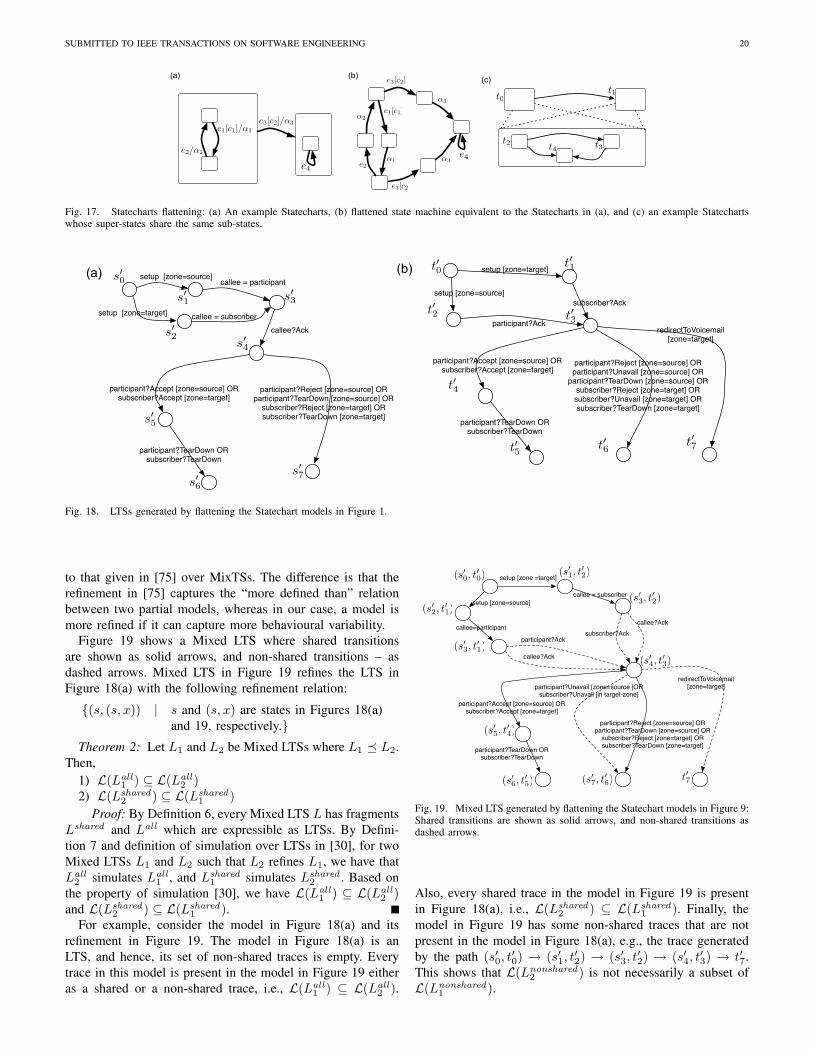
SUBMITTED TO IEEE TRANSACTIONS ON SOFTWARE ENGINEERING 20
e1[c1]/!1
e2/!2
e3[c2]/!3
e4
(a) (b) (c)
t0t1
t2 t3t4
e1[c1]
!1e2
!2
e3[c2]
!3e4
e3[c2]
!3
Fig. 17. Statecharts flattening: (a) An example Statecharts, (b) flattened state machine equivalent to the Statecharts in (a), and (c) an example Statechartswhose super-states share the same sub-states.
setup [zone=source]
callee?Ack
participant?Reject [zone=source] ORparticipant?TearDown [zone=source] OR
subscriber?Reject [zone=target] ORsubscriber?TearDown [zone=target]
participant?TearDown ORsubscriber?TearDown
participant?Accept [zone=source] ORsubscriber?Accept [zone=target]
setup [zone=target]
setup [zone=target]
setup [zone=source]
participant?Ack
subscriber?Ack
redirectToVoicemail[zone=target]
participant?Reject [zone=source] ORparticipant?Unavail [zone=source] OR
participant?TearDown [zone=source] ORsubscriber?Reject [zone=target] ORsubscriber?Unavail [zone=target] ORsubscriber?TearDown [zone=target]
participant?TearDown ORsubscriber?TearDown
participant?Accept [zone=source] ORsubscriber?Accept [zone=target]
s!0
s!1
s!2
s!3
s!4
s!5
(a) t!0 t!1
t!2 t!3
t!4
t!5 t!6 t!7
(b)
callee = subscriber
callee = participant
s!6
s!7
Fig. 18. LTSs generated by flattening the Statechart models in Figure 1.
to that given in [75] over MixTSs. The difference is that therefinement in [75] captures the “more defined than” relationbetween two partial models, whereas in our case, a model ismore refined if it can capture more behavioural variability.
Figure 19 shows a Mixed LTS where shared transitionsare shown as solid arrows, and non-shared transitions – asdashed arrows. Mixed LTS in Figure 19 refines the LTS inFigure 18(a) with the following refinement relation:
{(s, (s, x)) | s and (s, x) are states in Figures 18(a)and 19, respectively.}
Theorem 2: Let L1 and L2 be Mixed LTSs where L1 � L2.Then,
1) L(Lall1 ) ⊆ L(Lall
2 )2) L(Lshared
2 ) ⊆ L(Lshared1 )
Proof: By Definition 6, every Mixed LTS L has fragmentsLshared and Lall which are expressible as LTSs. By Defini-tion 7 and definition of simulation over LTSs in [30], for twoMixed LTSs L1 and L2 such that L2 refines L1, we have thatLall
2 simulates Lall1 , and Lshared
1 simulates Lshared2 . Based on
the property of simulation [30], we have L(Lall1 ) ⊆ L(Lall
2 )and L(Lshared
2 ) ⊆ L(Lshared1 ).
For example, consider the model in Figure 18(a) and itsrefinement in Figure 19. The model in Figure 18(a) is anLTS, and hence, its set of non-shared traces is empty. Everytrace in this model is present in the model in Figure 19 eitheras a shared or a non-shared trace, i.e., L(Lall
1 ) ⊆ L(Lall2 ).
setup [zone =target]
setup [zone=source]
participant?Ack subscriber?Ack
redirectToVoicemail[zone=target]
participant?Reject [zone=source] ORparticipant?TearDown [zone=source] OR
subscriber?Reject [zone=target] ORsubscriber?TearDown [zone=target]participant?TearDown OR
subscriber?TearDown
participant?Accept [zone=source] ORsubscriber?Accept [zone=target]
callee?Ack
callee?Ack
callee = subscriber
callee=participant
participant?Unavail [zone=source ]ORsubscriber?Unavail [in target-zone]
(s!0, t
!0)
(s!2, t
!1)
(s!1, t
!2)
(s′3, t
′1)
(s!3, t
!2)
(s!4, t
!3)
(s!5, t
!4)
(s!6, t
!5) (s!
7, t!6) t!7
Fig. 19. Mixed LTS generated by flattening the Statechart models in Figure 9:Shared transitions are shown as solid arrows, and non-shared transitions asdashed arrows.
Also, every shared trace in the model in Figure 19 is presentin Figure 18(a), i.e., L(Lshared
2 ) ⊆ L(Lshared1 ). Finally, the
model in Figure 19 has some non-shared traces that are notpresent in the model in Figure 18(a), e.g., the trace generatedby the path (s′0, t
′0) → (s′1, t
′2) → (s′3, t
′2) → (s′4, t
′3) → t′7.
This shows that L(Lnonshared2 ) is not necessarily a subset of
L(Lnonshared1 ).
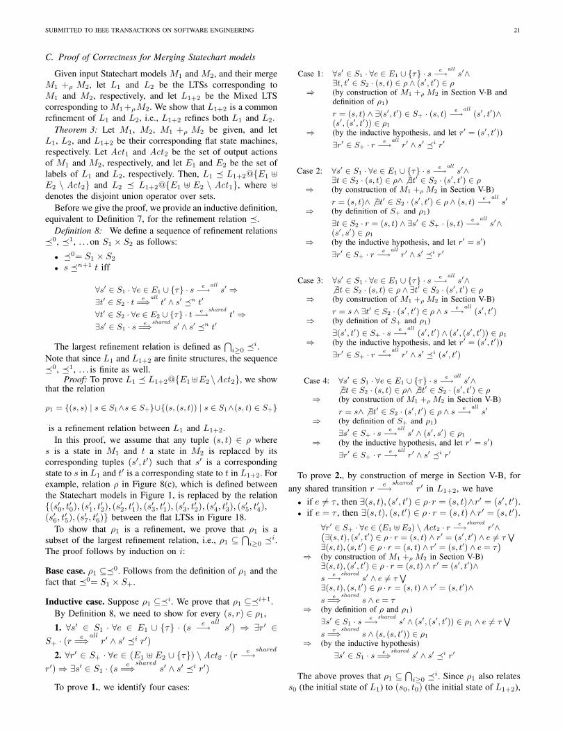
SUBMITTED TO IEEE TRANSACTIONS ON SOFTWARE ENGINEERING 21
C. Proof of Correctness for Merging Statechart models
Given input Statechart models M1 and M2, and their mergeM1 +ρ M2, let L1 and L2 be the LTSs corresponding toM1 and M2, respectively, and let L1+2 be the Mixed LTScorresponding to M1 +ρM2. We show that L1+2 is a commonrefinement of L1 and L2, i.e., L1+2 refines both L1 and L2.
Theorem 3: Let M1, M2, M1 +ρ M2 be given, and letL1, L2, and L1+2 be their corresponding flat state machines,respectively. Let Act1 and Act2 be the set of output actionsof M1 and M2, respectively, and let E1 and E2 be the set oflabels of L1 and L2, respectively. Then, L1 � L1+2@{E1 ]E2 \ Act2} and L2 � L1+2@{E1 ] E2 \ Act1}, where ]denotes the disjoint union operator over sets.
Before we give the proof, we provide an inductive definition,equivalent to Definition 7, for the refinement relation �.
Definition 8: We define a sequence of refinement relations�0, �1, . . . on S1 × S2 as follows:
• �0= S1 × S2
• s �n+1 t iff
∀s′ ∈ S1 · ∀e ∈ E1 ∪ {τ} · se−→
alls′ ⇒
∃t′ ∈ S2 · te
=⇒allt′ ∧ s′ �n t′
∀t′ ∈ S2 · ∀e ∈ E2 ∪ {τ} · te−→
sharedt′ ⇒
∃s′ ∈ S1 · se
=⇒shared
s′ ∧ s′ �n t′
The largest refinement relation is defined as⋂i≥0 �i.
Note that since L1 and L1+2 are finite structures, the sequence�0, �1, . . . is finite as well.
Proof: To prove L1 � L1+2@{E1]E2 \Act2}, we showthat the relation
ρ1 = {(s, s) | s ∈ S1∧s ∈ S+}∪{(s, (s, t)) | s ∈ S1∧(s, t) ∈ S+}
is a refinement relation between L1 and L1+2.In this proof, we assume that any tuple (s, t) ∈ ρ where
s is a state in M1 and t a state in M2 is replaced by itscorresponding tuples (s′, t′) such that s′ is a correspondingstate to s in L1 and t′ is a corresponding state to t in L1+2. Forexample, relation ρ in Figure 8(c), which is defined betweenthe Statechart models in Figure 1, is replaced by the relation{(s′0, t′0), (s′1, t
′2), (s′2, t
′1), (s′3, t
′1), (s′3, t
′2), (s′4, t
′3), (s′5, t
′4),
(s′6, t′5), (s′7, t
′6)} between the flat LTSs in Figure 18.
To show that ρ1 is a refinement, we prove that ρ1 is asubset of the largest refinement relation, i.e., ρ1 ⊆
⋂i≥0 �i.
The proof follows by induction on i:
Base case. ρ1 ⊆�0. Follows from the definition of ρ1 and thefact that �0= S1 × S+.
Inductive case. Suppose ρ1 ⊆�i. We prove that ρ1 ⊆�i+1.By Definition 8, we need to show for every (s, r) ∈ ρ1,
1. ∀s′ ∈ S1 · ∀e ∈ E1 ∪ {τ} · (s e−→alls′) ⇒ ∃r′ ∈
S+ · (r e=⇒allr′ ∧ s′ �i r′)
2. ∀r′ ∈ S+ · ∀e ∈ (E1 ] E2 ∪ {τ}) \ Act2 · (r e−→shared
r′)⇒ ∃s′ ∈ S1 · (s e=⇒shareds′ ∧ s′ �i r′)
To prove 1., we identify four cases:
Case 1: ∀s′ ∈ S1 · ∀e ∈ E1 ∪ {τ} · se−→
alls′∧
∃t, t′ ∈ S2 · (s, t) ∈ ρ ∧ (s′, t′) ∈ ρ⇒ (by construction of M1 +ρM2 in Section V-B and
definition of ρ1)r = (s, t) ∧ ∃(s′, t′) ∈ S+ · (s, t)
e−→all
(s′, t′)∧(s′, (s′, t′)) ∈ ρ1
⇒ (by the inductive hypothesis, and let r′ = (s′, t′))∃r′ ∈ S+ · r
e−→allr′ ∧ s′ �i r′
Case 2: ∀s′ ∈ S1 · ∀e ∈ E1 ∪ {τ} · se−→
alls′∧
∃t ∈ S2 · (s, t) ∈ ρ∧ 6 ∃t′ ∈ S2 · (s′, t′) ∈ ρ⇒ (by construction of M1 +ρM2 in Section V-B)
r = (s, t)∧ 6 ∃t′ ∈ S2 · (s′, t′) ∈ ρ ∧ (s, t)e−→
alls′
⇒ (by definition of S+ and ρ1)∃t ∈ S2 · r = (s, t) ∧ ∃s′ ∈ S+ · (s, t)
e−→alls′∧
(s′, s′) ∈ ρ1
⇒ (by the inductive hypothesis, and let r′ = s′)∃r′ ∈ S+ · r
e−→allr′ ∧ s′ �i r′
Case 3: ∀s′ ∈ S1 · ∀e ∈ E1 ∪ {τ} · se−→
alls′∧
6 ∃t ∈ S2 · (s, t) ∈ ρ ∧ ∃t′ ∈ S2 · (s′, t′) ∈ ρ⇒ (by construction of M1 +ρM2 in Section V-B)
r = s ∧ ∃t′ ∈ S2 · (s′, t′) ∈ ρ ∧ se−→
all(s′, t′)
⇒ (by definition of S+ and ρ1)∃(s′, t′) ∈ S+ · s
e−→all
(s′, t′) ∧ (s′, (s′, t′)) ∈ ρ1
⇒ (by the inductive hypothesis, and let r′ = (s′, t′))∃r′ ∈ S+ · r
e−→allr′ ∧ s′ �i (s′, t′)
Case 4: ∀s′ ∈ S1 · ∀e ∈ E1 ∪ {τ} · se−→
alls′∧
6 ∃t ∈ S2 · (s, t) ∈ ρ∧ 6 ∃t′ ∈ S2 · (s′, t′) ∈ ρ⇒ (by construction of M1 +ρM2 in Section V-B)
r = s∧ 6 ∃t′ ∈ S2 · (s′, t′) ∈ ρ ∧ se−→
alls′
⇒ (by definition of S+ and ρ1)∃s′ ∈ S+ · s
e−→alls′ ∧ (s′, s′) ∈ ρ1
⇒ (by the inductive hypothesis, and let r′ = s′)∃r′ ∈ S+ · r
e−→allr′ ∧ s′ �i r′
To prove 2., by construction of merge in Section V-B, forany shared transition r e−→shared
r′ in L1+2, we have• if e 6= τ , then ∃(s, t), (s′, t′) ∈ ρ·r = (s, t)∧r′ = (s′, t′).• if e = τ , then ∃(s, t), (s, t′) ∈ ρ · r = (s, t)∧ r′ = (s, t′).
∀r′ ∈ S+ · ∀e ∈ (E1 ] E2) \Act2 · re−→
sharedr′∧`
∃(s, t), (s′, t′) ∈ ρ · r = (s, t) ∧ r′ = (s′, t′) ∧ e 6= τW
∃(s, t), (s, t′) ∈ ρ · r = (s, t) ∧ r′ = (s, t′) ∧ e = τ´
⇒ (by construction of M1 +ρM2 in Section V-B)∃(s, t), (s′, t′) ∈ ρ · r = (s, t) ∧ r′ = (s′, t′)∧s
e−→shared
s′ ∧ e 6= τW
∃(s, t), (s, t′) ∈ ρ · r = (s, t) ∧ r′ = (s, t′)∧s
e=⇒
shareds ∧ e = τ
⇒ (by definition of ρ and ρ1)∃s′ ∈ S1 · s
e−→shared
s′ ∧ (s′, (s′, t′)) ∈ ρ1 ∧ e 6= τW
sτ
=⇒shared
s ∧ (s, (s, t′)) ∈ ρ1
⇒ (by the inductive hypothesis)∃s′ ∈ S1 · s
e=⇒
shareds′ ∧ s′ �i r′
The above proves that ρ1 ⊆⋂i≥0 �i. Since ρ1 also relates
s0 (the initial state of L1) to (s0, t0) (the initial state of L1+2),
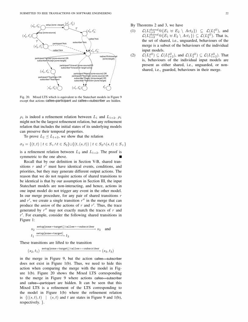
SUBMITTED TO IEEE TRANSACTIONS ON SOFTWARE ENGINEERING 22
setup [zone =target]
setup [zone=source]
participant?Ack subscriber?Ack
redirectToVoicemail[zone=target]
participant?Reject [zone=source] ORparticipant?TearDown [zone=source] OR
subscriber?Reject [zone=target] ORsubscriber?TearDown [zone=target]
participant?TearDown ORsubscriber?TearDown
participant?Accept [zone=source] ORsubscriber?Accept [zone=target]
callee?Ack
callee?Ack
!
!
participant?Unavail [zone=source]ORsubscriber?Unavail [in target-zone]
(s!0, t
!0)
(s′2, t
′1)
(s′1, t
′2)
(s′3, t
′1)
(s!3, t
!2)
(s!4, t
!3)
(s!5, t
!4)
(s!6, t
!5) (s!
7, t!6) t!7
Fig. 20. Mixed LTS which is equivalent to the Statechart models in Figure 9except that actions callee=participant and callee==subscriber are hidden.
ρ1 is indeed a refinement relation between L1 and L1+2. ρ1
might not be the largest refinement relation, but any refinementrelation that includes the initial states of its underlying modelscan preserve their temporal properties.
To prove L2 � L1+2, we show that the relation
σ2 = {(t, t) | t ∈ S+∧t ∈ S2}∪{(t, (s, t)) | t ∈ S2∧(s, t) ∈ S+}is a refinement relation between L2 and L1+2. The proof issymmetric to the one above.
Recall that by our definition in Section V-B, shared tran-sitions r and r′ must have identical events, conditions, andpriorities, but they may generate different output actions. Thereason that we do not require actions of shared transitions tobe identical is that by our assumption in Section III, the inputStatechart models are non-interacting, and hence, actions inone input model do not trigger any event in the other model.In our merge procedure, for any pair of shared transitions rand r′, we create a single transition r′′ in the merge that canproduce the union of the actions of r and r′. Thus, the tracegenerated by r′′ may not exactly match the traces of r andr′. For example, consider the following shared transitions inFigure 1:
s2setup[zone=target]/callee==subscriber−−−−−−−−−−−−−−−−−−−−−−−−−→ s3 and
t1setup[zone=target]−−−−−−−−−−−−→ t3
These transitions are lifted to the transition
(s2, t1)setup[zone=target]/callee==subscriber−−−−−−−−−−−−−−−−−−−−−−−−−→ (s3, t3)
in the merge in Figure 9, but the action callee==subscriberdoes not exist in Figure 1(b). Thus, we need to hide thisaction when comparing the merge with the model in Fig-ure 1(b). Figure 20 shows the Mixed LTS correspondingto the merge in Figure 9 where actions callee==subscriberand callee==participant are hidden. It can be seen that thisMixed LTS is a refinement of the LTS corresponding tothe model in Figure 1(b) where the refinement relationis {((s, t), t) | (s, t) and t are states in Figure 9 and 1(b),respectively. }.
By Theorems 2 and 3, we have(1) L(Lshared
1+2 @{E1 ] E2 \ Act2}) ⊆ L(Lall1 ), and
L(Lshared1+2 @{E1 ] E2 \ Act1}) ⊆ L(Lall
2 ). That is,the set of shared, i.e., unguarded, behaviours of themerge is a subset of the behaviours of the individualinput models.
(2) L(Lall1 ) ⊆ L(Lall
1+2), and L(Lall2 ) ⊆ L(Lall
1+2). Thatis, behaviours of the individual input models arepresent as either shared, i.e., unguarded, or non-shared, i.e., guarded, behaviours in their merge.