Embed Size (px)
Citation preview

Submitted toIEEE TRANSACTIONS ON VISUALIZATION AND COMPUTER GRAPHICS 1
Texturing FluidsVivek Kwatra David Adalsteinsson Theodore Kim Nipun Kwatra1 Mark Carlson2 and Ming Lin
UNC Chapel Hill 1Georgia Institute of Technology 2DNA Productions
Abstractmdash We present a novel technique for synthesizing tex-tures over dynamically changing fluid surfaces We use bothimage textures as well as bump maps as example inputs Imagetextures can enhance the rendering of the fluid by eitherimparting realistic appearance to it or by stylizing it whereasbump maps enable the generation of complex micro-structureson the surface of the fluid that may be very difficult to synthesizeusing simulation To generate temporally coherent textures overa fluid sequence we transport texture information ie color andlocal orientation between free surfaces of the fluid from onetime step to the next This is accomplished by extending thetexture information from the first fluid surface to the 3D fluiddomain advecting this information within the fluid domain alongthe fluid velocity field for one time step and interpolating it backonto the second surface ndash this operation in part uses a novelvector advection technique for transporting orientation vectorsWe then refine the transported texture by performing texturesynthesis over the second surface using our ldquosurface textureoptimizationrdquo algorithm which keeps the synthesized texturevisually similar to the input texture and temporally coherentwith the transported one We demonstrate our novel algorithmfor texture synthesis on dynamically evolving fluid surfaces inseveral challenging scenarios
Index Termsmdash Texture Synthesis Fluid Simulation SurfacesVector Advection
I I NTRODUCTION
REALISTIC modeling simulation and rendering of fluidmedia have applications in various domains including
special effects computer animation electronic games en-gineering visualization and medical simulation Often thecomputational expense involved in simulating complex fluidphenomena limit the spatio-temporal resolution at which thesesimulations can be performed This limitation makes it ex-tremely difficult to synthesize complex fine-resolution micro-structures on the free surface of the fluid that are usuallypresent in many commonly occurring fluid phenomena Ex-amples of such micro-structures include small-scale waves ina river stream foam and bubbles in turbulent water patternsin lava flow etc Even with a highly robust and sophisticatedfluid simulation system capable of modeling such structuresit is quite difficult to control the shape and appearance ofthese structures within the simulation We explore an alter-native approach which makes use of examples or samples offluid shape and appearance to aid and complement the fluidsimulation process
An important aspect of synthesizing fluid animations is therendering and visualization of the fluid In order to renderthe desired appearance of the fluid one needs to accuratelymodel the material properties of the fluid In general it is non-trivial to model these properties since they depend on multiplefactors like density temperature viscosity turbulence etc
Additionally these properties tend to vary across the surfaceof the fluid as well as over time Typically these materialproperties behave like a textureie the fluid appearanceconsists of local features that are statistically self-similar overspace and time Even though these features diffuse as theymove along with the fluid they also re-generate over timeensuring that statistically the appearance of the fluid featuresremains the same We exploit this property of fluid behaviorby obtaining example textural images of the fluid of interestand using them to render the appearance of the fluid Figure 1demonstrates an example where the appearance of lava flowingover a mountain is made much more interesting by renderingit with texture Our technique also provides a new way ofvisualizing surface properties of the fluid like flow and shapeby exposing them using the appearance and evolution of thesynthesized texture
Textures have been extensively used to impart novel appear-ance to static surfaces either by synthesizing texture over aplane and wrapping it over the surface or by directly syn-thesizing the texture over surfaces However extending thesetechniques for texturing a surface that is dynamically changingover time is a non-trivial problem This is so because oneneeds to maintain temporal coherence and spatial continuityof the texture over time while making sure that the texturalelements or features that compose the texture maintain theirvisual appearance even as the entire texture evolves Such ageneral technique would also aid in creation of special effectswith fluid phenomena where the effect involves texturing afluid surface with arbitrary textures (as shown in Figure 9)Additionally it has potential applications in the visualizationof vector fields and motion of deformable bodieseg thevelocity field of the fluid near its free surface is made apparentby the continuously evolving texture
A Main Results
In this paper we present a novel texture synthesis algorithmfor fluid flows We assume that we have available a fluidsimulator which is capable of generating free surfaces of thesimulated fluid medium as well as providing the fluid velocityfield We develop a technique for performing texture synthesison the free surface of the fluid by synthesizing texture colorson pointsplaced on the surface This is motivated by previousmethods for synthesizing texture directly on surfaces [1]ndash[3] However these approaches typically grow the texturepoint-by-point over the surface We extend and generalize theidea of texture optimization [4] to handle synthesis over 3Dsurfaces Consequently ours is a global technique where thetexture over the entire surface is evolved simultaneously acrossmultiple iterations
Submitted toIEEE TRANSACTIONS ON VISUALIZATION AND COMPUTER GRAPHICS 2
(A) (B) (C)
Fig 1
LAVA SCENE RENDERED WITH AND WITHOUT FLUID TEXTURING (A) SHOWS A FRAME FROM A LAVA ANIMATION RENDERED WITHOUT ANY TEXTURE
SYNTHESIZED OVER IT WHILE (B) AND (C) SHOW THE SAME FRAME RENDERED AFTER TEXTURING USING TWO DIFFERENT LAVA TEXTURES
In order to maintain temporal coherence between movingsurfaces in different time steps we need to ensure that thetexture synthesized on consecutive surfaces is similar to eachother We achieve this goal by first transporting the texture onthe surface in the first time step to the next using the velocityfield of the fluid that was responsible for the transport of thesurface in the first place The transported surface texture is thenused as asoft constraintfor the texture optimization algorithmwhen synthesizing texture over the second surface The trans-port of texture across 3D surfaces is not as straightforward asadvecting pixels using 2D flow fields in the planar case sincethere is no obvious correspondence between points on the twosurfaces We establish the correspondence by first transferringtexture information (color andlocal orientation) from the firstsurface onto a uniform 3D grid followed by advection oftexture information on this grid using the velocity field ofthe fluid The advected texture is then interpolated back onthe second surface to complete the transport
Our approach has the following characteristics
bull It can work with any fluid simulator that provides the3D velocity fields and free surfaces of the fluid at eachiteration as output
bull It can take image textures bumpdisplacement maps aswell as alpha maps as input
bull It performs texture synthesis ondynamically evolving 3Dsurfaces as opposed to just 2D flow fields
bull It can handle significant topological changes in the sim-ulated fluids including merge and separation of multiplefluid volumes
bull It preserves thevisual similarity1 of the synthesized tex-ture to the input texture even while advecting both scalar(eg color) and vector quantities (local orientations) de-scribing the texture to maintain temporal coherence withrespect to the motion of the 3D fluid
Our technique for advection of vector quantities through avelocity field is a novel contribution which may have otherapplications as well It takes into account rotation undergoneby the vector when traveling through the velocity field inaddition to the translation We demonstrate our algorithm using
1Visual similarity refers to the spatial continuity and the resemblance ofvisual appearance between the input and synthesized textures See Section V-Bfor more details
a variety of textures on several scenes including a broken dama river scene and lava flow as shown in Figures 9 ndash 14
B Organization
The rest of the paper is organized as follows In Section IIwe briefly summarize the related work in relevant areasIn Section III we present an overview of our approachWe describe the pre-computation required to construct thenecessary data structures in Section IV and our generalizedtexture optimization technique on 3D surfaces in Section VWe then explain how we maintain temporal coherence of theresulting texture sequence by transporting texture informationbetween successive time steps in Section VI We show theresults of our system in Section VII Finally we concludewith some possible future research directions
II RELATED WORK
In this section we briefly summarize recent advances in theresearch areas relevant to our work
A Example-based Texture Synthesis
Texture synthesis has been widely investigated in computergraphics Various approaches are known including pixel-based [5] [6] patch-based [7]ndash[9] and global synthesis [4][10]ndash[12] techniques Patch-based techniques usually obtainhigher synthesis quality than pixel-based methods Globaltechniques provide the most control especially when coupledwith an intuitive cost metric and are therefore most desirablefor fluid texturing Our synthesis algorithm is based on aglobal texture optimization technique [4] which achieves anice blend of quality and flexibility by working with patchsizes of varying degree from large to small
An important class of texture synthesis techniques relevantto our work is that concerned with surface texture synthesiswhere texture is synthesized directly over a 3D surface Theprimary issues that arise here include representation of thetexture and neighborhood construction and parameterizationfor performing search in the input texture Turk [1] andWei and Levoy [2] represent texture by storing color and localsurface orientation on points uniformly distributed over thesurface Ying et al [3] parameterize the surface locally onto
Submitted toIEEE TRANSACTIONS ON VISUALIZATION AND COMPUTER GRAPHICS 3
the plane to compute a texture atlas which is then used toperform synthesis in the plane Praun et al [13] also performlocal patch parameterizations for generating lapped texturesThe technique of Maillot et al [14] is significant in thecontext of surface parameterization for texture mapping Forpoint based representations texture neighborhoods need to beconstructed on the fly While in [1] surface marching is used tocompute the neighborhood in [2] the mesh vertices are locallyparameterized onto the plane to form each neighborhood Weuse both kinds of neighborhoods in our work (see Section V-Afor more details)
B Flow-Guided Texturing and Visualization
Kwatra et al [4] introduced a new technique for 2Dtexture synthesis based on iterative optimization They alsodemonstrate how the same technique can be used for flow-guided texture animation where a planar flow field is usedto guide the motion of texture elements in a synthesized2D texture sequence We solve the fluid texturing problemby adapting ideas from the texture optimization technique toperform texture synthesis directly on a dynamically changingtriangulated surface in 3D ndash the motion of the surface beingguided by a 3D fluid simulation as opposed to a planarflow field Recently Lefebvre and Hoppe [15] have alsodemonstrated texture advection on the plane and on staticsurfaces using appearance-space texture synthesis
Bhat et al [16] presented a flow-based video synthesistechnique by enforcing temporal continuity along a set of user-specific flow lines While this method focus on stationary flowfields with focuses on video editing our algorithm is applica-ble to any time-varyingdynamicflow fields generated by fluidsimulators and use image textures as input In addition weuse the simulated flow fields as a mechanism to automaticallycontrol and guide constrained texture synthesis while theirsrequires user input to specify the flow lines to edit the videosequences
Wiebe and Houston [17] and Rasmussen et al [18] performfluid texturing by advecting texture coordinates along the flowfield using level sets and particles respectively Howeverthey do not address the issue of regeneration of textureat places of excessive stretch or compression Neyret [19]proposed a method for applying stochastic textures to fluidflows that avoids a variety of visual artifacts and demonstratedinteresting 2D and 3D animations produced by coherent ad-vection of the applied texture This approach works in regulardomains (2D or 3D) and the textures employed are primarilystochastic or procedural in nature to avoid blending artifactsOur technique on the other hand is concerned with synthesison thefree surfaceof the fluid and can handle a wider varietyof textures
There has been work in the scientific visualization commu-nity that makes use of texture for visualization and represen-tation of vector fields [20] as well as shape [21] We observethat in a similar spirit our technique can also be used forvisualization of surface velocity fields as well as motion ofdeformable bodies usingarbitrary textures
C Fluid Simulation and Flows on Arbitrary Surfaces
Simulation of fluids and various related natural phenomenahave received much recent attention Foster and Metaxas [22]and Stam [23] were among the pioneers in using full 3DNavier-Stokes differential equations for generating fluid ani-mations in computer graphics Level set methods [24] [25]have been developed for tracking and rendering the freesurface of the fluid Specialized techniques for synthesizingdetailed fluid phenomena like drops bubbles and foam etcdirectly through simulation have also been researched [26]ndash[28] In the context of our work fluid simulation is treated asa black box where its outputs namely the 3D velocity fieldand the free surface are used by our algorithm to transporttexture information between successive frames and synthesizethe texture on the fluid surface respectively
Recently Stam [29] Shi and Yu [30] have proposed methodsto simulate Navier-Stokes flows on 2D meshes Stamrsquos methodrequires the surface to be a regular quadrilateral mesh whileShi and Yursquos technique works on any triangulated meshBoth focused on the goal of generating plausible 2D flowson surfaces embedded in 3D space In contrast we presenttechniques for performingtexture synthesison dynamicallymoving 3D surfaces Our approach can alleviate commonartifacts that occur in simple passive advection of texturecoordinates and color as detailed in [19]
Bargteil et al [31] present a semi-Lagrangian surface track-ing method for tracking surface characteristics of a fluidsuch as color or texture coordinates In a similar manner ourwork also relies on fluid surface transport to advect color andother texture properties However in addition to these scalarquantities we also track the orientation vectors on the fluidsurface through the velocity field These vectors are tracked toensure that the synthesized texture has consistent orientationacross (temporally) nearby free surfaces
In work concurrent to ours Bargteil et al [32] [33] havealso developed a similar technique for texturing liquid anima-tions Our neighborhood construction and search techniquesas well as our orientation advection method are different fromtheir work Our work was also presented as atechnical sketchin SIGGRAPH 2006 [34]
III OVERVIEW
We couple controllable texture synthesis with fluid simu-lation to perform spatio-temporally coherent fluid texturingThe main elements of our system include (i) a fluid simulatorfor generating the dynamic surface with velocity information(ii) a technique for performing texture synthesis on the fluidsurface coherent with temporally neighboring surfaces and(iii) a method for transporting texture information from onesurface to the other Figure 2 shows a flow chart of howthese three components interact with each other for fluidtexturing The surface texture synthesis module hands thetextured surface over to the texture transporter which in turntransports texture information along the velocity field for asingle time step and hands this information back to thesynthesis module
The only requirements for a fluid simulator to work withour system are that it should be able to output the 3D fluid
Submitted toIEEE TRANSACTIONS ON VISUALIZATION AND COMPUTER GRAPHICS 4
Fluid Simulator
Texture Transporter
Surface TextureSynthesis
SurfaceVelocity Field
InitializationConstraint
TexturedSurface
Fig 2
OVERVIEW OF OUR FLUID TEXTURE SYNTHESIS SYSTEM
velocity field at each iteration and that the surfaces generatedduring each iteration should be a consequence of transportingthe surface at the previous iteration through the fluid velocityfield over a single time step In our simulator the surfaces aregenerated as the level set of an advected distance function
We start by obtaining the free surface of the fluid for the firsttime step and then texture this surface using our surface textureoptimization algorithm (explained in Section V) We thentransport the texture to the fluid surface for the second timestep using our texture transport technique The transportedquantities include the texture colors (and any other associatedproperties like surface displacement transparency etc) as wellas local orientation vectors that are needed to synthesize thetexture on the 3D surface
This transported texture serves two purposes Firstly it actsas an initialization for the texture on the surface for the secondtime step Secondly it is treated as asoft constraintwhichspecifies that the synthesized texture on the second surfaceshould stay as close as possible to this initialized texture Oursurface texture optimization technique can naturally handlethis constraint by plugging it into a texture cost function Thesetwo operations of transport and synthesis are then repeated foreach time step of the simulation
IV SURFACE PREPARATION
To perform texture synthesis on a 3D surface one needsto take into account the fact that there is no regular gridof pixels available as is the case in an image Hence werepresent the texture on a surface by assigning color valuesto points placed on the surface These points serve the samepurpose on a surface as pixels do in an image However inthe case of an image pixels lie on a uniform grid On theother hand it is impossible to specify a single uniform grid ofpoints on an arbitrary surface Even so we want the points tobe as uniformly spaced as possible to ensure uniform texturesampling on the surface
Before we begin synthesis we prepare the surface forsynthesis by having the following constructs in place Firstlywe place the desired number of points on the surface in away that they sample the surface uniformly These pointsare connected to form an auxiliary triangle mesh that aidsin interpolation and neighborhood construction Secondly a
smooth vector field is computed over this mesh that definesthe local orientation (2D coordinate system) at each pointon the surface2 The orientation field is used to map 3Dpoints on the surface onto 2D points in a plane This mappingis later used for comparing a surface patch against a pixelneighborhood in the input image These operations are mostlysimilar to previous work but we describe them here brieflyfor completeness
A Point Placement and Mesh Hierarchy
As discussed above we store texture information (colorand local orientation) in points placed on the surface beingtextured Hence the number of points will determine theres-olution of the synthesized texture For example a surface with10000 points will be equivalent to an image of size 100times100pixels An important thing to note is that the resolution of thesurface changes from frame to frame If the area of the surfaceincreases the points also increases in number proportionallyand vice-versa The starting number of points is a user-definedparameter but it is computed automatically for subsequentframes We want the points to be spaced as uniformly aspossible over the surface so that the synthesized texture alsohas a uniform quality throughout A consequence of this needfor uniformity (and the non-constant nature of the number ofpoints over time) is that the points for each free surface (intime) are generated independently Fortunately our grid-basedtexture color and orientation advection techniques obviate theneed to track the points explicitly
We generate the points in a hierarchical fashion to representthe texture at varying resolutions We follow the procedure ofTurk [1] At each level we initialize the points by placing themrandomly over the surface mesh and then use the surface-restricted point repulsion procedure of Turk [35] to achieveuniform spacing between these points Once we have placedthe points we connect them to generate a triangulated meshfor each level of the hierarchy We use the mesh re-tilingprocedure of [36] for re-triangulating the original surface meshusing the new points We use the Triangle library [37] fortriangulation at each intermediate step
B Local Orientation
The next step is the computation of a local orientation ateach point placed on the surface We want these orientations tovary smoothly over each mesh in the hierarchy We use a polarspace representation of the orientation field as proposed byZhang et al [38] Firstly a polar map is computed for eachpoint on the mesh A polar map linearly transforms anglesdefined between vectors on the surface of the mesh to anglesbetween vectors in a 2D polar space The transformation issimply φ = θ times2πΘ whereθ is the angle in mesh spaceΘ is the total face angle around a point andφ is the polar
2The curved nature of the surface implies that a unique vector cannot beused to define the 2D coordinate system at each point on the surface ndash unlikethe case with a plane This is due to the fact the coordinate system needsto lie in the tangent plane of the surface which itself changes from point topoint Consequently we need to define an orientation vectorfield spread overthe entire surface
Submitted toIEEE TRANSACTIONS ON VISUALIZATION AND COMPUTER GRAPHICS 5
space angle (shown in the Figure 3A) The orientation vector ateach point can now be represented as an angle in polar spaceThis representation allows us to easily smooth the orientationfield by diffusion across adjacent points for two points onthe mesh connected by an edge we want their orientations tomake the same polar angle with the common edge betweenthem as shown in Figure 3B Thus each diffusion operationaverages the current orientation angle of a point with theangles determined through the points connected to it In amesh hierarchy this diffusion is performed at the coarsest levelfirst and then propagated up the hierarchy The orientationfield is initialized to be the zero polar angle everywhere afterwhich multiple iterations of smoothing are performed Notethat an orientation angle can be converted into a 3D orientationvector by first applying the reverse transformation (of theone described above) to obtain a mesh space angle The 3Dorientation vector at the point is then obtained by rotating apre-definedreferencevector stored at that point by this meshspace angle This reference vector sits in the tangent plane ofthe point ie lies perpendicular to thenormal at the pointand is designated as having azeropolar angle
θ1
θ2
θ3
θ4θ5
θ6
φ5
φ6
φ4 φ3
φ2φ1
Θ = Σθi φi = θi times 2πΘ(A)
β
2
d2
α
1
d1
(B)
Fig 3
(A) M APPING ANGLES FROM MESH SPACE TO POLAR SPACE
(B) ORIENTATIONS d1 AND d2 SHOULD MAKE SIMILAR polar ANGLES (α
AND β RESPECTIVELY) WITH THE COMMON EDGE BETWEEN THEM
V SURFACE TEXTURE SYNTHESIS
Once we have constructed the mesh hierarchy and theorientation field we are ready to perform synthesis In thissection we will describe the two essential steps in perform-ing surface texture synthesis neighborhood construction andsurface texture optimization
A Neighborhood Construction
Texture synthesis operations primarily require matchinginput and output pixel neighborhoods with each other Aswe discussed in the previous section a uniform grid of
pixels is not always available on the surface All we haveis a unstructured mesh of points Therefore we need tomatch unstructured point neighborhoods against gridded pixelneighborhoods
In earlier approaches for surface texture synthesis thisproblem is solved by either pre-computing a mapping from thesurface to a plane using texture atlases [3] or by construct-ing local neighborhoods over the surface on the fly throuheither surface marching [1] or construction of local parame-terizations [2] Pre-computing the mapping from surface toplane gives nicer neighborhoods but is tedious to computeespecially for a sequence of surfaces We favor anon the flyapproach because of its simplicity and scalability in handlinga sequence of meshes
We construct two types of neighborhoods on the meshwhich we refer to aspixel neighborhoodsand vertex neigh-borhoodsrespectively These two types of neighborhoods areused to interpolate color information back and forth betweenvertices3 on the mesh and pixels in the (image) plane Pixelneighborhoods are used to transfer information from meshspace to image space while vertex neighborhoods perform thereverse operation transferring information from image spaceto mesh space
1) Pixel NeighborhoodA pixel neighborhood is definedas a set of points on the mesh whose 2D coordinates in thelocal orientation space around a central point map to integerlocations in the plane also the neighborhood is bounded by awidth w which implies that if(i j) are the 2D coordinates of apoint in the neighborhood thenminusw2le i j lew2 Given theorientation field we have a coordinate system in the tangentplane of the surface mesh that we can use to march along thesurface The orientation directiond defines one axis of thecoordinate system while the second axist (orthonormal tod)is obtained as the cross product between the normal at thesurface point andd4 We use this coordinate system to marchalong the surface in a fashion similar to [1] adding all surfacepoints corresponding to valid integer pixel locations to thepixel neighborhood Once a pixel neighborhood is constructedit can be used to interpolate colors from mesh space to imagespace For example the color of the pixel at(i j) is computedusing barycentric interpolation of colors associated with thecorners of the triangle in which the corresponding point liesFigure 4 shows a pixel neighborhood mapped onto the surfaceof a triangle mesh
2) Vertex NeighborhoodA vertex neighborhood in a meshis defined as the set of vertices connected to each other andlying within a certaingeodeisc distancendash distance measuredin the local orientation space of the mesh ndash to a central vertexGiven the vertexc as the center the 2D location of a vertexin its neighborhood is computed as its displacement fromcalong the orientation field on the mesh For a givenpixelneighborhood widthw we include only those vertices incrsquos
3we use the termvertex here to distinguish it from the termpoint usedearlier A point can be any point on the surface where asverticesrefer tothe set of points that are part of a triangle mesh that is being used to sampleand represent the surface
4vertex normals areinterpolatedfrom incident faces and the normal at apoint is interpolated from vertex normals of the containing face
Submitted toIEEE TRANSACTIONS ON VISUALIZATION AND COMPUTER GRAPHICS 6
2D 3D
Fig 4
PIXEL NEIGHBORHOOD CONSTRUCTION A 2D PIXEL NEIGHBORHOOD IS MAPPED ONTO POINTS ON THE TRIANGLE MESH THE RED ARROW IS THE
ORIENTATION VECTOR WHILE THE BLUE ARROW IS ITS ORTHONORMAL COMPLEMENT THE POINT CORRESPONDING TO ANY GIVEN PIXEL IN THE
NEIGHBORHOOD LIKE THE ONE SHOWN AS A GREEN CIRCLE LIES ON A SINGLE TRIANGLE OF THE MESH AS SHOWN ON THE RIGHT THIS TRIANGLE IS
USED TO DETERMINE TEXTURE INFORMATION AT THE GIVEN PIXEL THROUGH BARYCENTRIC INTERPOLATION
neighborhood whose displacement vector(l1 l2) measuredstarting atc is such thatminusw2 lt l1 l2 lt w2 To computedisplacements of vertices in the neighborhood ofc we employa local mesh flattening procedure similar to the one usedin [2] [13] We first consider all vertices in the 1-ring ofcie vertices that are directly connected toc If d representsthe orientation vector atc and t represent its orthonormalcomplement then the displacement vector of a vertexv inthe 1-ring ofc is (v middotdv middot t) wherev = (vminusc)σ Hereσ isthe scaling factor between mesh space and image space Wethen keep moving outwards to the 2-ring and so on until allneighborhood vertices are exhausted Generally on a curvedsurface the displacement vector computed for a vertex willdepend on the path one takes to reach that vertex Hence foreach vertex we compute its displacement as the average ofthose predicted by its neighbors and also run a relaxationprocedure to ensure an even better fit for the displacements
Once a point neighborhood is constructed it can be used tointerpolate colors from image space to mesh space Since thedisplacement of each vertex in the neighborhood correspondsto real-valued 2D coordinates we use bilinear interpolationof colors at nearby integer locations in the image space todetermine the color of the vertex Figure 5 shows a vertexneighborhood where a set of connected points on the meshare mapped onto the 2D plane
B Surface Texture Optimization
Our approach for synthesizing texture on a 3D surfaceis motivated by the texture optimization algorithm proposedby Kwatra et al [4] Their formulation is valid only on a2D plane We extend that formulation to handle synthesison a arbitrary 3D surface The reason for using such anoptimization algorithm for synthesis is that we want it tonaturally handle synthesis on a dynamic surface maintainingtemporal coherence between consecutive surfaces and spatialcoherence with the texture for each individual surface We canincorporate the transported texture from the previous surfaceas a soft constraint with the optimization approach
The optimization proceeds by minimizing an energy func-tion that determines the quality of the synthesized texturewith respect to the input texture example as well as the
transported texture from previous surface We first considerthe energy with respect to just the input example This energyis defined in terms of the similarity between localvertexneighborhoods of the textured surface andimage-space pixelneighborhoods of the input texture example To compare thesetwo incongruous neighborhoods we first interpolate colorsfrom the image-space pixel neighborhood onto real-valued2D locations corresponding to the vertex neighborhood asdescribed in Section V-A2 We then define the textureenergy for a single vertex neighborhood to be the sum ofsquared differences between the colors of mesh vertices andthe interpolated input colors at the vertex locations The totalenergy of the textured surface is equal to the sum of energiesover individual neighborhoods of the surface IfS denotes thesurface being textured andZ denotes the input texture samplethen the texture energy overS is defined as
Et(szp) = sumpisinSdagger
spminuszp2 (1)
Heres is the vectorized set of color values for all vertices ofthe meshsp is the set of colors associated with vertices in avertex neighborhood around the vertexp zp contains colorsfrom a pixel neighborhood inZ interpolated at 2D locationscorresponding to the vertex neighborhood aroundp The inputtexture neighborhood from whichzp is interpolated is the onethat appears most similar to thepixel neighborhood aroundp ndash which is constructed as explained in Section V-A1 ndashunder the sum of squared differences It should be noted thateven though our energy formulation is described completelyin terms of vertex neighborhoods we need to resort to pixelneighborhoods during search for efficiency
The set of verticesSdagger around which neighborhoods areconstructed is a subset of the set of all vertices inS Sdagger
is chosen such that there is a significant overlap betweenall neighborhoodsie a single point occurs within multipleneighborhoods See Figure 6 for a schematic explanation ofhow the texture energy is computed
The energy function defined above measures the spatialconsistency of the synthesized surface texture with respectto the input texture example To ensure that the synthesizedtexture is temporally coherent as well we add another term
Submitted toIEEE TRANSACTIONS ON VISUALIZATION AND COMPUTER GRAPHICS 7
2D3D
Fig 5
VERTEX NEIGHBORHOOD CONSTRUCTION A SET OF CONNECTED POINTS ON THE MESH ARE MAPPED ONTO THE2D PLANE THE ORIENTATION
VECTOR AT THE CENTRAL VERTEX ALIGNS ITSELF WITH THE PRIMARY AXIS OF THE PLANE EACH VERTEX MAPS TO A REAL-VALUED 2D LOCATION AS
SHOWN EXPLICITLY FOR THE YELLOW CIRCLED VERTEX GIVEN A PLANAR PIXEL NEIGHBORHOOD THE COLOR AT A MESH VERTEX IS DETERMINED
THROUGH BILINEAR INTERPOLATION OF THE FOUR PIXELS THAT ITS2D MAPPED LOCATION LIES BETWEEN
which measures the similarity of the textured surface to thetexture transported from the previous time step The trans-ported texture already specifies a color value vector denotedasc corresponding to each vertex location inS We treatc asa soft constraint ons ie we want the color of the transportedtexture and synthesized texture to be close to each other Thecorresponding energy function is
Ec(sc) = sumkisinS
λk(s(k)minusc(k))2 (2)
where k iterates over all vertices in the mesh andλk is aweighting factor that controls the influence of transported tex-ture color at a vertex over its synthesized value We typicallyuse a gradient based weighting scheme where a larger weightis given to the transported texture color at a vertex that hasgreater color gradient in its vicinity Note that we also usecas an initialization fors The total energy of the textured fluidsurface is
E(x) = Et(xzp)+Ec(xc)
The algorithm proceeds by optimizing this total energy ofthe surface being textured in an iterative fashion Given aninitialization of the texture ndash random for the first frame andtransported from the previous surface for the remaining ndash thefollowing steps are repeated until convergence
1) For each vertexpisin Sdagger construct a vertex neighborhoodsp and a pixel neighborhoodxp in the vicinity of pfrom the current surface textures Assign colors to thepixels in xp through barycentric interpolation on themesh (Section V-A)
2) Find the closest input texture neighborhood sayxprimepfor each pixel neighborhoodxp constructed above andinterpolatexprimep at real-valued 2D locations correspondingto the vertices insp to obtain the interpolated inputneighborhoodzp
3) Re-compute the surface texture colorss by minimizingthe total energyE(szp) with respect tos keeping theset of interpolated input neighborhoodszp fixed Forthe squared energy function used here this correspondsto simply taking a weighted average of the colorspredicted by the different neighborhoods affecting a
point as well as the colors obtained from the transportedtexture
Note that when performing synthesis in a multi-resolutionfashion the optimization first proceeds at the coarsest level ofthe mesh hierarchy This is followed by an up-sampling step inwhich the finer level mesh vertices copy the color values fromtheir coarser level counterparts followed by diffusion of thesecolor values at the finer level This acts as the initialization forthe finer mesh after which optimization proceeds as earlierAlso we typically use more than one neighborhood size ateach level In our experiments we run three optimizationpasses that use neighborhoods of size 33times33 17times17 and9times9 pixels respectively in that order
VI T EXTURE TRANSPORT
We now describe the texture transport procedure whichtransports texture information from the currently synthesizedsurface to the next surface in the time sequence The textureinformation being transported includes two quantities (i) thetexture color (or any other properties being synthesized likedisplacement transparency etc) and (ii) the orientation vectorfield on the surface While the texture color is what we reallywant to transport it is necessary to transport the orientationfield also because that determines how the texture neighbor-hoods are oriented on the surface when synthesis is performedIf the orientation fields on two consecutive surfaces are notconsistent it would be very difficult to find neighborhoods inthe input texture that match the transported texture
A Color Advection
Our approach for transporting the texture color is basedon standard advection techniques that have been well studiedin the level set literature The basic idea is to perform thetransfer on a volumetric grid as opposed to directly betweensurfaces This volumetric grid is the same as that used bythe fluid simulation to represent the velocity field One mightbe tempted to simply advect the texture colors from the firstsurface to the next However since the resolution of the gridis typically much smaller than the number of points used insynthesis this will result in loss of texture resolution Hence
Submitted toIEEE TRANSACTIONS ON VISUALIZATION AND COMPUTER GRAPHICS 8
Texture Energy(Single Neighborhood)
(A)
Total Texture Energy = Σ Individual Neighborhood Energy(B)
Fig 6
TEXTURE ENERGY (A) SHOWS THE TEXTURE ENERGY FOR A SINGLE VERTEX NEIGHBORHOOD IT IS THE SQUARED COLOR-SPACE DISTANCE BETWEEN
THE GIVEN VERTEX NEIGHBORHOOD AND ITS CLOSEST MATCH IN THE INPUT IMAGE TEXTURE (B) SHOWS THE TOTAL TEXTURE ENERGY FOR THE
SURFACE TEXTURE IT IS SIMPLY THE SUM OF ENERGIES OF INDIVIDUAL NEIGHBORHOODS
we advect 3D vertex coordinates instead of texture colorbecause vertex coordinates can usually be safely interpolatedwithout loss of resolution Advection of 3D coordinates isconceptually equivalent to back-tracking each point in thevolumetric grid to its source location in the previous time-stepFor a given vertex in the new mesh one can obtain its back-tracked location by interpolating from nearby grid points Itstexture color is then obtained through barycentric interpolationover the triangle closest to this back-tracked location Thevarious steps are enumerated in order below
1) The first step is to determine the 3D coordinates at gridlocations This is quite simple the coordinates are thelocation of the grid point itself since the surface andthe grid sit in the same space
2) Next we treat each component of the coordinate fieldas a scalar field Each scalar field is advected along thevelocity field for a single time step This step is doneby solving the following advection update equation
partϕ
part t=minusu middotnablaϕ (3)
whereϕ is the scalar being advectedu is the velocityfield obtained from the fluid simulation andnablaϕ is thespatial gradient of the scalar field We save the fluidvelocity field at all intermediate time steps that thesimulation may have stepped through and use those
steps while performing the advection update as wellThe update is performed using a first order upwindscheme [39]
3) After the advection is complete we have the advectedcoordinates at each grid point These coordinates areinterpolated onto the vertices of the new surface corre-sponding to the next time step Each new surface vertexnow knows which location it came from in the previoustime step through these back-tracked coordinates
4) Finally we assign a color (or other property) valueto each new vertex as the color of the back-trackedlocation Letx be the back-tracked location The color ofx is obtained by first finding the pointp on the previoussurface that is nearest tox We compute the color ofp through barycentric interpolation of the colors at thecorners of the triangle on whichp lies This color isthen also used as the color for the back-tracked locationx To speed up the search for the nearest surface pointswe use a hash table to store the triangles of the mesh
It should be noted that the backtracked coordinates may not al-ways be close to the surface in which case the projection ontothe surface may return undesirable texture color values How-ever our texture synthesis algorithm automatically handles thisby pastingover the bad regions with new input patches thatare visually consistent with the surrounding regions
Submitted toIEEE TRANSACTIONS ON VISUALIZATION AND COMPUTER GRAPHICS 9
B Orientation Advection
VelocityField
Vector AdvectionScalar Advection
OriginalOrientation
(A)
1
2
d
u1
u2
d + (u2- u1)∆t
dnablau
(B)
Fig 7
(A) TRANSPORTING AN ORIENTATION VECTOR BY ONLY ADVECTING ITS
SCALAR COMPONENTS WILL(INCORRECTLY) ONLY TRANSLATE THE
VECTOR OUR VECTOR ADVECTION TECHNIQUE CORRECTLY TRANSPORTS
THE VECTOR BY TRANSLATING AS WELL AS ROTATING IT (B) THE
ORIENTATION VECTORd BETWEEN POINTS1 AND 2 GETS DISTORTED AS A
FUNCTION OF THE GRADIENT OF THE VELOCITY FIELD ALONGd
The transport of orientations is not as straightforward asthe transport of color This is because orientations are vectorswhich may rotate as they move along the velocity field Ifwe simply advect each scalar components of the orientationvector independently then it would only translate the vectorFigure 7A shows the difference in the result obtained byscalar vs vector advection Conceptually to preform vectoradvection we can advect the tail and head of the orientationvector separately through the field and use the normalizedvector from the advected tail to the advected head as the neworientation vector This operation needs to be performed inthe limit that the orientation is of infinitesimal lengthie thehead tends to the tail This results in a modified analyticaladvection equation of the form
partdpart t
=minusu middotnablad+(I minusddT)d middotnablau (4)
Here the first termminusu middotnablad is the scalar advection term asapplied to each component of the orientation vectord Theterm d middotnablau computes the derivative of velocityu along theorientation d As shown in Figure 7Bd gets distorted bythe velocity field because its head and tail undergo differentdisplacements This difference in displacements is governedby the difference in the velocity values at the head and thetail which is simply the velocity field gradientnablau alongthe orientationd Finally since we are only interested in thedirection of thed and not its magnitude we need to normalize
the distortion so that it reduces to a rotation This is achievedthrough the term(IminusddT) which is a projection operator thatprojectsd middotnablau to the plane perpendicular tod This projectionessentially ensures that in differential termsd always stays aunit vector
To perform advection ofd we follow similar steps as forscalar advection with the following changes In step 1 weextendthe orientation field from the surface onto the grid usingthe technique of [40] The orientation vectors are propagatedoutwards from the surface along the surface normal onto thegrid The advection update step 2 solves (4) again usingupwind differencing this time alternating between the twoterms in the equation For step 3 we directly interpolate theadvected orientations on new surface points and normalizethem These vectors are then converted into the polar anglerepresentation described in Section IV We typically re-run thediffusion algorithm to smoothen the orientation field Note thatunlike texture color the orientation field is smooth to beginwith hence loss of resolution is not a concern Therefore weinterpolate it directly without any need to go through step 4
VII R ESULTS
We have implemented the techniques presented here in C++and rendered the results using 3DelightRcopy We use a grid-based method for fluid simulation [23] [41] [42] Howeverour technique is general enough to work with other typesof simulators like finite volume based techniques [43] Weapplied our implementation on several challenging scenarioswith several different textures (shown in Figure 8)
Fig 8
TEXTURE EXEMPLARS USED IN OUR RESULTS LAST TWO ARE BUMP-MAP
TEXTURES USED WITH THE RIVER
The first scene is a broken-dam simulation as shown inFigure 9 and Figure 10 where a large volume of water isdropped into a tank of water causing the invisible wall to breakand the simulated water to splash The water surface is stylizedusing various different textures in the shown examples In theaccompanied video note that the texture on the surface is splitand merged seamlessly as the surface undergoes substantialtopological changes Figure 11A shows a comparison of ourresult for this simulation with the result obtained throughpure advection (ie no texture synthesis after the first frame)
Submitted toIEEE TRANSACTIONS ON VISUALIZATION AND COMPUTER GRAPHICS 10
Fig 9
BROKEN-DAM A LARGE VOLUME OF WATER IS DROPPED INTO A BROKEN DAM CAUSING THE WATER TO SPLASH THE WATER SURFACE IS STYLIZED
USING A GREEN SCALES TEXTURE THE TEXTURE FEATURES ON THE SURFACE SPLIT AND MERGE NICELY AS THE SURFACE UNDULATES THE
VIEWPOINT IS ROTATING AROUND THE SCENE
Even though advecting the texture ensures perfect temporalcoherence the visual quality of the texture is lost due todiffusion
The second simulation is a river scene shown in Figure 12and Figure 13 where the water flows down the stream andcarries the surface texture with it In Figure 12A we show theriver with a bump mapped texture which creates the impressionof small scale waves on the surface of the river Figure 12Bshows the same scene with a different bump texture that givesthe impression of rocks floating in the river Figure 12C usesthe same texture as Figure 12B but treats it as a transparencytexture coupled with color to give the impression of floatingleaves on the river surface Figure 11B compares the renderingof a frame of the bump mapped river with the renderingof the original fluid surface generated by the simulation Itshould be easy to see that the texture adds a lot of detail andmicro-structure to the river which is missing from the originalsurface
The third simulation is that of lava flow shown in Figure 14in which lava flows from the top of the mountain downwardsonto the walls Results are shown for four different texturesThe first two examples are more realistic while the last twoare stylistic
The computational complexity of our algorithm is dom-inated by nearest neighbor search during texture synthesisand mesh hierarchy construction during surface preparationDepending upon the number of points used for the mesh hi-erarchy construction takes between 3minus15 minutes per frame5However the mesh hierarchy is computed offline for eachsimulation so that runtime costs include only surface texture
5Only one level of hierarchy is constructed for all frames of the animationsubsequent to the first one which uses three levels
synthesis and texture transport We accelerate the nearestneighbor search by using a hierarchical clustering of the imageneighborhoods The synthesis times depend on the simulationbecause the number of points on the mesh change linearly withthe area of the mesh as it evolves Our average synthesis timesare approximately 60 seconds per frame for the broken dam90 seconds per frame for the river scene and 200 secondsper frame for the lava flow The number of points used forstoring texture pixels varied in the range of 100000 pointsand 500000 points over the course of the simulation
The supplementary videos include the results for riverlava and broken dam examples We also show a comparisonbetween the results of our technique and the results obtainedby using pure advection as well as comparisons with resultsobtained without using any texture synthesis at all All ourresults are also available online athttpgammacsunceduTexturingFluids
VIII D ISCUSSIONamp FUTURE WORK
We have presented a novel synthesis algorithm for advectingtextures on dynamically changing fluid surfaces over timeOur work successfully demonstrates transport of textures along3D fluid flows which undergo complex topological changesbetween successive frames while preserving visual similaritybetween the input and the output textures We define visualsimilarity through a cost function that then drives a surfacetexture optimization process We achieve fluid texturing bycombining this surface texture optimization process with anadvection scheme based on a level-set method for trackingthe surface characteristics We also explicitly model and solvefor the advection of vector quantities like surface orientationthrough the velocity field
Submitted toIEEE TRANSACTIONS ON VISUALIZATION AND COMPUTER GRAPHICS 11
Fig 10
BROKEN-DAM RENDERED USING DIFFERENT TEXTURE EXEMPLARS
One can envision using our technique as a renderingmechanism in conjunction with fluid simulation techniquesIt can be used to enhance the complexity of the synthesizedfluid phenomena by adding surface micro-structures such aswaves and eliminating the need to manually model photomet-ric properties of materials such as lava Another interestingapplication is flow visualization Our technique synthesizestexture sequences that animate the input texture as controlledby the fluid flows obtained from a fluid simulator Hence itcan facilitate flow visualization using a rich variety of textures
A limitation of our technique which is relevant to surfacetexture synthesis in general is that it is often impossibleto define an orientation vector field on the surface that issmooth everywhere Overlapping neighborhoods near singu-larity points like sources sinks and vortices of the field maynot align well with each other because computation of the2D mapping of vertices becomes unstable in these regionsThis can sometimes cause excessive blurring near singularitypoints
Currently the texture synthesis process is agnostic of anyproperties of the fluid surface that may affect its appearanceFor example one might want the appearance of the texture tobe affected in a certain way by vortices and high curvatureregions on the fluid surface As part of future research wewould like to add to our technique the ability to incorporatesuch relationships into the synthesis process Among otherfuture directions we would like to extend our approach tohandle 3D volume textures as well as video textures
REFERENCES
[1] G Turk ldquoTexture synthesis on surfacesrdquo inSIGGRAPH rsquo01 Proceed-ings of the 28th annual conference on Computer graphics and interactivetechniques New York NY USA ACM Press 2001 pp 347ndash354
[2] L-Y Wei and M Levoy ldquoTexture synthesis over arbitrary manifoldsurfacesrdquo inSIGGRAPH rsquo01 Proceedings of the 28th annual conferenceon Computer graphics and interactive techniques New York NY USAACM Press 2001 pp 355ndash360
[3] L Ying A Hertzmann H Biermann and D Zorin ldquoTexture andshape synthesis on surfacesrdquo inProceedings of the 12th EurographicsWorkshop on Rendering Techniques London UK Springer-Verlag2001 pp 301ndash312
[4] V Kwatra I Essa A Bobick and N Kwatra ldquoTexture optimizationfor example-based synthesisrdquoACM SIGGRAPH vol 24 no 3pp 795ndash802 August 2005 appears in ACM Transactions onGraphics (TOG) [Online] Available httpwwwccgatecheducplprojectstextureoptimization
[5] A Efros and T Leung ldquoTexture synthesis by non-parametric samplingrdquoin International Conference on Computer Vision 1999 pp 1033ndash1038
[6] L-Y Wei and M Levoy ldquoFast texture synthesis using tree-structuredvector quantizationrdquoProceedings of ACM SIGGRAPH 2000 pp 479ndash488 July 2000 iSBN 1-58113-208-5
[7] A A Efros and W T Freeman ldquoImage quilting for texture synthesisand transferrdquoProceedings of SIGGRAPH 2001 pp 341ndash346 2001
[8] L Liang C Liu Y-Q Xu B Guo and H-Y Shum ldquoReal-time texturesynthesis by patch-based samplingrdquoACM Transactions on Graphicsvol Vol 20 No 3 pp 127ndash150 July 2001
[9] V Kwatra A Schodl I Essa G Turk and A Bobick ldquoGraphcuttextures Image and video synthesis using graph cutsrdquoACMSIGGRAPH vol 22 no 3 pp 277ndash286 July 2003 appearsin ACM Transactions on Graphics (TOG) [Online] Availablehttpwwwccgatecheducplprojectsgraphcuttextures
[10] R Paget and I D Longstaff ldquoTexture synthesis via a noncausalnonparametric multiscale markov random fieldrdquoIEEE Transactions onImage Processing vol 7 no 6 pp 925ndash931 June 1998
[11] W T Freeman T R Jones and E C Pasztor ldquoExample-based super-resolutionrdquoIEEE Comput Graph Appl vol 22 no 2 pp 56ndash65 2002
[12] Y Wexler E Shechtman and M Irani ldquoSpace-time video completionrdquoin CVPR 2004 2004 pp 120ndash127
[13] E Praun A Finkelstein and H Hoppe ldquoLapped texturesrdquoProc ofACM SIGGRAPH pp 465ndash470 2000
[14] J Maillot H Yahia and A Verroust ldquoInteractive texture mappingrdquoin SIGGRAPH rsquo93 Proceedings of the 20th annual conference onComputer graphics and interactive techniques New York NY USAACM Press 1993 pp 27ndash34
[15] S Lefebvre and H Hoppe ldquoAppearance-space texture synthesisrdquo in
Submitted toIEEE TRANSACTIONS ON VISUALIZATION AND COMPUTER GRAPHICS 12
(A)
(B)
Fig 11
(A) COMPARISON WITH PURE ADVECTION OUR RESULT IS SHOWN ON THE LEFT WHILE THE RESULT OF ADVECTION IS SHOWN ON THE RIGHT
(B) COMPARING THE RIVER SCENE RENDERED WITH FLUID TEXTURING ON THE LEFT AND WITHOUT ANY TEXTURE ON THE RIGHT
SIGGRAPH rsquo06 ACM SIGGRAPH 2006 Papers New York NY USAACM Press 2006 pp 541ndash548
[16] K S Bhat S M Seitz J K Hodgins and P K Khosla ldquoFlow-based video synthesis and editingrdquoACM Transactions on Graphics(SIGGRAPH 2004) vol 23 no 3 August 2004
[17] M Wiebe and B Houston ldquoThe tar monster Creating a character withfluid simulationrdquo in Proceedings of the SIGGRAPH 2004 Conferenceon Sketches amp Applications ACM Press 2004
[18] N Rasmussen D Enright D Nguyen S Marino N Sumner W GeigerS Hoon and R Fedkiw ldquoDirectable photorealistic liquidsrdquo inSCA rsquo04Proceedings of the 2004 ACM SIGGRAPHEurographics symposium onComputer animation 2004 pp 193ndash202
[19] F Neyret ldquoAdvected texturesrdquoProc of ACM SIGGRAPH Eurograph-ics Symposium on Computer Animation pp 147ndash153 2003
[20] F Taponecco and M Alexa ldquoVector field visualization using markovrandom field texture synthesisrdquo inVISSYM rsquo03 Proceedings of thesymposium on Data visualisation 2003 Aire-la-Ville SwitzerlandSwitzerland Eurographics Association 2003 pp 195ndash202
[21] G Gorla V Interrante and G Sapiro ldquoTexture synthesis for 3dshape representationrdquoIEEE Transactions on Visualization and ComputerGraphics vol 9 no 4 pp 512ndash524 2003
[22] N Foster and D Metaxas ldquoRealistic animation of liquidsrdquoGraphicalmodels and image processing GMIP vol 58 no 5 pp 471ndash4831996 [Online] Available citeseernjneccomfoster95realistichtml
[23] J Stam ldquoStable fluidsrdquo inSiggraph 1999 Computer GraphicsProceedings A Rockwood Ed Los Angeles Addison WesleyLongman 1999 pp 121ndash128 [Online] Available citeseernjneccomstam99stablehtml
[24] N Foster and R Fedkiw ldquoPractical animations of liquidsrdquo inSIGGRAPH 2001 Computer Graphics Proceedings E Fiume Ed
ACM Press ACM SIGGRAPH 2001 pp 23ndash30 [Online] Availableciteseernjneccomfoster01practicalhtml
[25] D Enright S Marschner and R Fedkiw ldquoAnimation and rendering ofcomplex water surfacesrdquo inProceedings of the 29th annual conferenceon Computer graphics and interactive techniques ACM Press 2002pp 736ndash744
[26] J-M Hong and C-H Kim ldquoAnimation of bubbles in liquidrdquo inCompGraph Forum vol 22 no 3 2003 pp 253ndash263
[27] T Takahashi H Fujii A Kunimatsu K Hiwada T Saito K Tanakaand H Ueki ldquoRealistic animation of fluid with splash and foamrdquo inComp Graph Forum vol 22 no 3 2003 pp 391ndash401
[28] H Wang P J Mucha and G Turk ldquoWater drops on surfacesrdquoACMTrans Graph vol 24 no 3 pp 921ndash929 2005
[29] J Stam ldquoFlows on surfaces of arbitrary topologyrdquoACM Trans onGraphics (Proc of ACM SIGGRAPH) 2003
[30] L Shi and Y Yu ldquoInviscid and incompressible fluid simulation ontriangle meshesrdquoJournal of Computer Animation and Virtual Worldsvol 15 no 3ndash4 pp 173ndash181 2004
[31] A W Bargteil T G Goktekin J F OrsquoBrien and J A Strain ldquoA semi-lagrangian contouring method for fluid simulationrdquoACM Transactionson Graphics vol 25 no 1 2006
[32] A W Bargteil F Sin J E Michaels T G Goktekin and J F OrsquoBrienldquoA texture synthesis method for liquid animationsrdquoACM SIGGRAPH2006 Technical Sketches July 2006
[33] mdashmdash ldquoA texture synthesis method for liquid animationsrdquoACM SIG-GRAPHEurographics Symposium on Computer Animation September2006
[34] V Kwatra D Adalsteinsson N Kwatra M Carlson and M LinldquoTexturing fluidsrdquo ACM SIGGRAPH 2006 Technical Sketches July2006
Submitted toIEEE TRANSACTIONS ON VISUALIZATION AND COMPUTER GRAPHICS 13
(A)
(B)
(C)
Fig 12
RIVER SCENE (SIDE-ON VIEW) RIVER SCENE WITH BUMP-MAP AND TRANSPARENCY TEXTURES CREATING THE IMPRESSION OF(A) SMALL SCALE
WAVES (B) FLOATING ROCKS AND (C) FLOATING LEAVES ON THE SURFACE OF THE RIVER
[35] G Turk ldquoGenerating textures on arbitrary surfaces using reaction-diffusionrdquo in SIGGRAPH rsquo91 Proceedings of the 18th annual con-ference on Computer graphics and interactive techniques New YorkNY USA ACM Press 1991 pp 289ndash298
[36] mdashmdash ldquoRe-tiling polygonal surfacesrdquo inSIGGRAPH rsquo92 Proceedingsof the 19th annual conference on Computer graphics and interactivetechniques New York NY USA ACM Press 1992 pp 55ndash64
[37] J R Shewchuk ldquoTriangle Engineering a 2d quality mesh generator anddelaunay triangulatorrdquo inFCRC rsquo96WACG rsquo96 Selected papers fromthe Workshop on Applied Computational Geormetry Towards GeometricEngineering London UK Springer-Verlag 1996 pp 203ndash222
[38] E Zhang K Mischaikow and G Turk ldquoVector field designon surfacesrdquo Georgia Institute of Technology Tech Rep 04-162004 [Online] Available httpwwwccgatechedugradszEugeneZhangvecflddesignhtml
[39] J Sethian ldquoLevel set methods and fast marching methods Evolvinginterfaces in computational geometryrdquo 1998 [Online] Availableciteseeristpsuedusethian99levelhtml
[40] D Adalsteinsson and J Sethian ldquoThe fast construction of extensionvelocities in level set methodsrdquoJournal of Computational Physics vol148 pp 2ndash22 1999
[41] M Griebel T Dornseifer and T NeunhoefferNumerical Simulation inFluid Dynamics A Practical Introduction ser SIAM Monographcs onMathematical Modeling and Computation SIAM 1990
[42] M Carlson P Mucha and G Turk ldquoRigid fluid Animating the interplaybetween rigid bodies and fluidrdquo inProc of the ACM SIGGRAPH ACMPress 2004
[43] R J LeVeque and D G CrightonFinite Volume Methods for Hy-perbolic Problems ser Cambridge Texts in Applied MathematicsCambridge University Press 2002
Submitted toIEEE TRANSACTIONS ON VISUALIZATION AND COMPUTER GRAPHICS 14
Fig 13
RIVER SCENE RENDERED WITH VARIOUS IMAGE TEXTURES
Fig 14
L AVA SCENE LAVA FLOWING ALONG A MOUNTAIN SHOWN WITH DIFFERENT TEXTURES
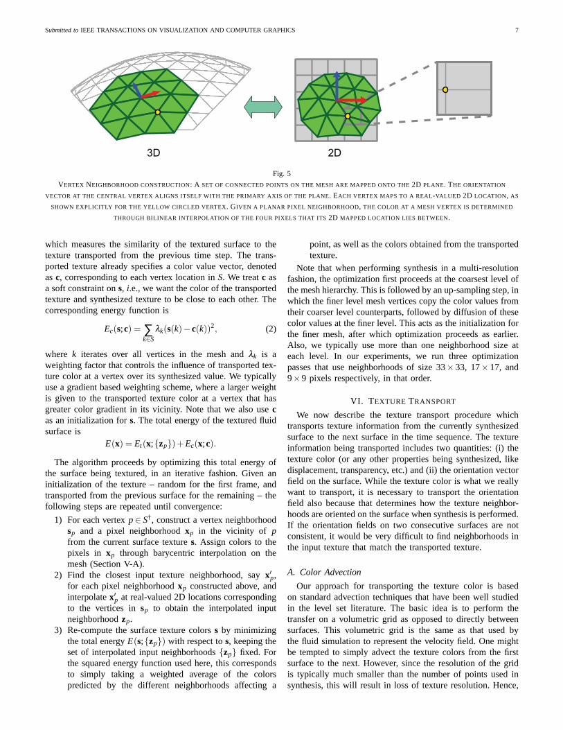
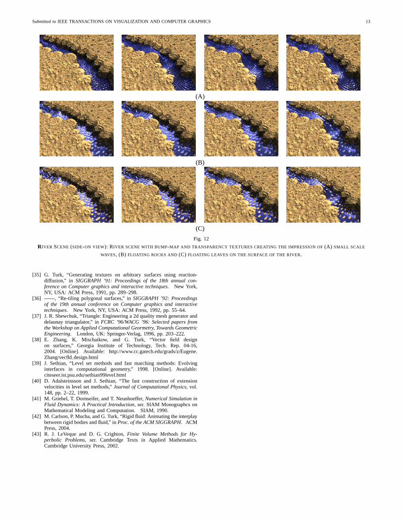
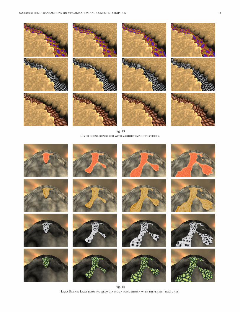
Submitted toIEEE TRANSACTIONS ON VISUALIZATION AND COMPUTER GRAPHICS 14
Fig 13
RIVER SCENE RENDERED WITH VARIOUS IMAGE TEXTURES
Fig 14
L AVA SCENE LAVA FLOWING ALONG A MOUNTAIN SHOWN WITH DIFFERENT TEXTURES