arX

iv:m

ath/

0212

212v

1 [

mat

h.O

C]

16

Dec

200

2SUBMITTED AS A REGULAR PAPER TO IEEE TRANSACTIONS ON ROBOTICS AND AUTOMATION 1

Coverage control for mobile sensing networksJorge Cortes, Sonia Martınez, Timur Karatas, Francesco Bullo, Member IEEE

Abstract—This paper presents control and coordination al-

gorithms for groups of vehicles. The focus is on autonomous

vehicle networks performing distributed sensing tasks where

each vehicle plays the role of a mobile tunable sensor. The

paper proposes gradient descent algorithms for a class of

utility functions which encode optimal coverage and sens-

ing policies. The resulting closed-loop behavior is adaptive,

distributed, asynchronous, and verifiably correct.

Keywords— Coverage control, distributed and asyn-

chronous algorithms, centroidal Voronoi partitions

I. Introduction

Mobile sensing networks

The deployment of large groups of autonomous vehi-cles is rapidly becoming possible because of technologicaladvances in networking and in miniaturization of electro-mechanical systems. In the near future large numbers ofrobots will coordinate their actions through ad-hoc com-munication networks and will perform challenging tasksincluding search and recovery operations, manipulation inhazardous environments, exploration, surveillance, and en-vironmental monitoring for pollution detection and esti-mation. The potential advantages of employing teams ofagents are numerous. For instance, certain tasks are diffi-cult, if not impossible, when performed by a single vehicleagent. Further, a group of vehicles inherently provides ro-bustness to failures of single agents or communication links.

Working prototypes of active sensing networks have al-ready been developed; see [1], [2], [3]. In [3], launchableminiature mobile robots communicate through a wirelessnetwork. The vehicles are equipped with sensors for vibra-tions, acoustic, magnetic, and IR signals as well as an activevideo module (i.e., the camera or micro-radar is controlledvia a pan-tilt unit). A second system is suggested in [4]under the name of Autonomous Oceanographic SamplingNetwork; see also [5], [6]. In this case, underwater vehi-cles are envisioned measuring temperature, currents, andother distributed oceanographic signals. The vehicles com-municate via an acoustic local area network and coordinatetheir motion in response to local sensing information and toevolving global data. This mobile sensing network is meantto provide the ability to sample the environment adaptively

Submitted on November 4, 2002. Previous short versions of thispaper appeared in the IEEE Conference on Robotics and Automation,Arlington, VA, May 2002, and Mediterranean Conference on Controland Automation, Lisbon, Portugal, July 2002.Jorge Cortes, Timur Karatas and Francesco Bullo are with the

Coordinated Science Laboratory, University of Illinois at Urbana-Champaign, 1308 W. Main St., Urbana, IL 61801, United States,Tels: +1-217-244-8734, +1-217-244-9414 and +1-217-333-0656, Fax:+1-217-244-1653, Email: jcortes,tkaratas,bullo@uiuc.eduSonia Martınez is with the Escola Universitaria Politecnica de Vi-

lanova i la Geltru, Universidad Politecnica de Cataluna, Av. V. Bal-aguer s/n, Vilanova i la Geltru, 08800, Spain, Tel: +34-938967720,Fax: +34-938967700, Email: soniam@mat.upc.es

in space and time. By identifying evolving temperatureand current gradients with higher accuracy and resolutionthan current static sensors, this technology could lead tothe development and validation of improved oceanographicmodels.

Optimal sensor allocation and coverage problems

A fundamental prototype problem in this paper is that ofcharacterizing and optimizing notions of quality-of-serviceprovided by an adaptive sensor network in a dynamic en-vironment. To this goal, we introduce a notion of sensorcoverage that formalizes an optimal sensor placement prob-lem. This spatial resource allocation problem is the sub-ject of a discipline called locational optimization [7], [8],[9], [10], [11].Locational optimization problems pervade a broad spec-

trum of scientific disciplines. Biologists rely on locationaloptimization tools to study how animals share territory andto characterize the behavior of animal groups obeying thefollowing interaction rule: each animal establishes a regionof dominance and moves toward its center. Locational opti-mization problems are spatial resource allocation problems(where to place mailboxes in a city or cache servers on theinternet) and play a central role in quantization and infor-mation theory (the design of a minimum-distortion fixed-rate vector quantizer is a locational problem). Other tech-nologies affected by locational optimization include meshand grid optimization methods, clustering analysis, datacompression, and statistical pattern recognition.Because locational optimization problems are so widely

studied, it is not surprising that methods are indeed avail-able to tackle coverage problems; see [7], [10], [12], [11].However, most currently-available algorithms are not ap-plicable to mobile sensing networks because they inherentlyassume a centralized computation for a limited size prob-lem in a known static environment. This is not the case inmulti-vehicle networks which, instead, rely on a distributedcommunication and computation architecture. Althoughan ad-hoc wireless network provides the ability to sharesome information, no global omniscient leader might bepresent to coordinate the group. The inherent spatially-distributed nature and limited communication capabilitiesof a mobile network invalidate classic approaches to algo-rithm design.

Distributed asynchronous algorithms for coverage control

In this paper we design coordination algorithms imple-mentable by a multi-vehicle network with limited sensingand communication capabilities. Our approach is relatedto the classic Lloyd algorithm from quantization theory;see [13] for a reprint of the original report and [14] for ahistorical overview. We present Lloyd descent algorithms

2 SUBMITTED AS A REGULAR PAPER TO IEEE TRANSACTIONS ON ROBOTICS AND AUTOMATION

that take into careful consideration all constraints on themobile sensing network. In particular, we design coveragealgorithms that are adaptive, distributed, asynchronous,and verifiably asymptotically correct:

Adaptive: Our coverage algorithms provide the networkwith the ability to address changing environments, sens-ing task, and network topology (due to agents departures,arrivals, or failures).Distributed: Our coverage algorithms are distributed in thesense that the behavior of each vehicle depends only onthe location of its neighbors. Also, our algorithms donot required a fixed-topology communication graph, i.e.,the neighborhood relationships do change as the networkevolves. The advantages of distributed algorithms are scal-ability and robustness.Asynchronous: Our coverage algorithms are amenable toasynchronous implementation. This means that the al-gorithms can be implemented in a network composed ofagents evolving at different speeds, with different compu-tation and communication capabilities. Furthermore, ouralgorithms do not require a global synchronization and con-vergence properties are preserved even if information aboutneighboring vehicles propagates with some delay. An ad-vantage of asynchronism is a minimized communicationoverhead.Verifiable Asymptotically Correct: Our algorithms guaran-tees monotonic descent of the cost function encoding thesensing task. Asymptotically the evolution of the mobilesensing network is guaranteed to converge to so-called cen-troidal Voronoi configurations that are critical points of theoptimal sensor coverage problem.

Let us describe in some detail what are the contribu-tions of this paper. Section II reviews certain locationaloptimization problems and their solutions as centroidalVoronoi partitions. Section III provides a continuous-timeversion of the classic Lloyd algorithm from vector quantiza-tion and applies it to the setting of multi-vehicle networks.In discrete-time, we propose a family of Lloyd algorithms.We carefully characterize convergence properties for bothcontinuous and discrete-time versions (Appendix VII col-lects some relevant facts on descent flows). We discuss aworst-case optimization problem, we investigate a simpleuniform planar setting, and we present numerical results.

Section IV presents two asynchronous distributed imple-mentations of Lloyd algorithm for ad-hoc networks withcommunication and sensing capabilities. Our treatmentcarefully accounts for the constraints imposed by the dis-tributed nature of the vehicle network. We present twoasynchronous implementations, one based on classic resultson distributed gradient flows, the other based on the struc-ture of the coverage problem.

Section V-A considers vehicle models with more realisticdynamics. We present two formal results on passive ve-hicle dynamics and on vehicles equipped with individuallocal controllers. We present numerical simulations of pas-sive vehicle models and of unicycle mobile vehicles. Next,Section V-B describes density functions that lead the multi-vehicle network to predetermined geometric patterns.

Review of distributed algorithms for cooperative control

Recent years have witnessed a large research effort fo-cused on motion planning and coordination problems formulti-vehicle systems. Issues include geometric patterns[15], [16], formation control [17], [18], [19], [20], [21], andconflict avoidance [22], [23]. Algorithms for robotic sens-ing tasks are presented for example in [24], [25]. It is onlyrecently, however, that truly distributed coordination lawsfor dynamic networks are being proposed; e.g., see [26], [27]and the conference versions of this work [28], [29].

Heuristic approaches to the design of interaction rulesand emerging behaviors have been throughly investigatedwithin the literature on behavior-based robotics; see [30],[31], [32], [17], [33], [34], [35], [36]. An example of coveragecontrol is discussed in [37]. Along this line of research, al-gorithms have been designed for sophisticated cooperativetasks. However, no formal results are currently availableon how to design reactive control laws, ensure their cor-rectness, and guarantee their optimality with respect to anaggregate objective.

The study of distributed algorithms is concerned withproviding mathematical models, devising precise specifica-tions for their behavior, and formally proving their cor-rectness and complexity. Via an automata-theoretic ap-proach, the references [38], [39] treat distributed consensus,resource allocation, communication, and data consistencyproblems. From a numerical optimization viewpoint, theworks in [40], [41], [42] discuss distributed asynchronous al-gorithms as networking algorithms, rate and flow control,and gradient descent flows. Typically, both these sets ofreferences consider networks with fixed topology, and donot address algorithms over ad-hoc dynamically changingnetworks. Another common assumption is that, any timean agent communicates its location, it broadcasts it to ev-ery other agent in the network. In our setting, this wouldrequire a non-distributed communication set-up.

II. From location optimization to centroidalVoronoi partitions

A. Locational optimization

In this section we describe a collection of known factsabout a meaningful optimization problem. References in-clude the theory and applications of centroidal Voronoipartitions, see [12], and the discipline of facility location,see [8]. Along the paper, we interchangeably refer to theelements of the network as sensors, agents, vehicles, orrobots.Let Q be a convex polytope in R

N and let ‖·‖ denote theEuclidean distance function. We call a map φ : Q → R+

a distribution density function if it represents a measureof information or probability that some event take placeover Q. In equivalent words, we can consider Q to be thebounded support of the function φ. Let P = (p1, . . . , pn)be the location of n sensors, each moving in the space Q.Because of noise and loss of resolution, the sensing per-formance at point q taken from ith sensor at the positionpi degrades with the distance ‖q − pi‖ between q and pi;

CORTES, MARTıNEZ, KARATAS AND BULLO: COVERAGE CONTROL FOR MOBILE SENSING NETWORKS 3

we describe this degradation with a non-decreasing differ-entiable function f : R+ → R+. Accordingly, f (‖q − pi‖)provides a quantitative assessment of how poor the sensingperformance is.Remark II.1: As an example, consider n mobile robots

equipped with microphones attempting to detect, identify,and localize a sound-source. How should we plan to robots’motion in order to maximize the detection probability? As-suming the source emits a known signal, the optimal detec-tion algorithm is a matched filter (i.e., convolve the knownwaveform with the received signal and threshold). Thesource is detected depending on the signal-to-noise-ratio,which is inversely proportional to the distance between themicrophone and the source. Various electromagnetic andsound sensors have signal-to-noise ratios inversely propor-tional to distance.Within the context of this paper, a partition of Q is a

collection of n polytopes W = W1, . . . ,Wn with disjointinteriors whose union is Q. We say that two partitionsW and W ′ are equal if Wi and W ′

i only differ by a set ofφ-measure zero, for all i ∈ 1, . . . , n.We consider the task of minimizing the locational opti-

mization function

H(P,W) =

n∑

i=1

∫

Wi

f(‖q − pi‖)dφ(q), (1)

where we assume that the ith sensor is responsible for mea-surements over its “dominance region” Wi. Note that thefunction H is to be minimized with respect to both (1)the sensors location P , and (2) the assignment of the dom-inance regions W . This problem is referred to as a fa-cility location problem and in particular as a continuousp-median problem in [8].Remark II.2: Note that if we interchange the positions of

any two agents, along with their associated regions of dom-inance, the value of the locational optimization function His not affected. To eliminate this discrete redundancy, onecould take the discrete group of permutations Σn with thenatural action on Qn, and consider Qn/Σn as the configu-ration space for the position P of the n vehicles.

B. Voronoi partitions

One can easily see that, at fixed sensors location, theoptimal partition of Q is the Voronoi partition V(P ) =V1, . . . , Vn generated by the points (p1, . . . , pn):

Vi = q ∈ Q | ‖q − pi‖ ≤ ‖q − pj‖ , ∀j 6= i.

We refer to [11] for a comprehensive treatment on Voronoidiagrams, and briefly present some relevant concepts. Theset of regions V1, . . . , Vn is called the Voronoi diagramfor the generators p1, . . . , pn. When the two Voronoiregions Vi and Vj are adjacent, pi is called a (Voronoi)neighbor of pj (and vice-versa). The set of indexes of theVoronoi neighbors of pi is denoted by N (i). Clearly, j ∈N (i) if and only if i ∈ N (j). We also define the (i, j)-faceas ∆ij = Vi ∩ Vj . Voronoi diagrams can be defined withrespect to various distance functions, e.g., the 1-, 2-, s-,

and ∞-norm over Q = Rm, and Voronoi diagrams can be

defined over Riemannian manifolds; see [43]. Some usefulfacts about the Euclidean setting are the following: if Q isa convex polytope in a N -dimensional Euclidean space, theboundary of each Vi is the union of (N − 1)-dimensionalconvex polytopes.

In what follows, we shall write

HV(P ) = H(P,V(P )).

Note that

HV(P ) =

∫

Q

mini∈1,...,n

f(‖q − pi‖)dφ(q) , (2)

= E

[

mini∈1,...,n

f(‖q − pi‖)

]

,

that is, the locational optimization function can be inter-preted as an expected value composed with a min opera-tion. This is the usual way in which the problem is pre-sented in the facility location and operations research lit-erature [8], [9]. Remarkably, one can show [12] that

∂HV

∂pi(P ) =

∂H

∂pi(P,V(P )) =

∫

Vi

∂

∂pif (‖q − pi‖) dφ(q),

(3)

and deduce some smoothness properties of HV . Sincethe Voronoi partition V depends at least continuously onP = (p1, . . . , pn), the function HV is at least continuouslydifferentiable.

C. Centroidal Voronoi partitions

Let us recall some basic quantities associated to a regionV ⊂ R

N and a mass density function ρ. The (generalized)mass, centroid (or center of mass), and polar moment ofinertia are defined as

MV =

∫

V

ρ(q) dq, CV =1

MV

∫

V

q ρ(q) dq,

JV,p =

∫

V

‖q − p‖2 ρ(q) dq.

Additionally, by the parallel axis theorem, one can write,

JV,p = JV,CV+MV ‖p− CV ‖

2 (4)

where JV,CV∈ R+ is defined as the polar moment of inertia

of the region V about its centroid.

Let us consider again the locational optimization prob-lem (1), and suppose now we are strictly interested in thesetting

H(P,W) =

n∑

i=1

∫

Wi

‖q − pi‖2dφ(q), (5)

that is, we assume f(‖q − pi‖) = ‖q − pi‖2. Applying theparallel axis theorem leads to simplifications for both the

4 SUBMITTED AS A REGULAR PAPER TO IEEE TRANSACTIONS ON ROBOTICS AND AUTOMATION

function HV and its partial derivative:

HV(P ) =

n∑

i=1

JVi,CVi+

n∑

i=1

MVi‖pi − CVi

‖2

∂HV

∂pi(P ) = 2MVi

(pi − CVi).

It is convenient to define HV,1 =∑n

i=1 JVi,CViand HV,2 =

∑n

i=1 MVi‖pi − CVi

‖2.Therefore, the (not necessarily unique) local minimum

points for the location optimization function HV are cen-troids of their Voronoi cells, i.e., each location pi satisfiestwo properties simultaneously: it is the generator for theVoronoi cell Vi and it is its centroid

CVi= argminpi

HV(P ).

Accordingly, the critical partitions and points for H arecalled centroidal Voronoi partitions. We will refer to a sen-sors configuration as a centroidal Voronoi configuration ifit gives rise to a centroidal Voronoi partition. This discus-sion provides a proof alternative to the one given in [12] forthe necessity of centroidal Voronoi partitions as solutionsto the continuous p-median location problem.

III. Continuous and Discrete-Time LloydDescent for Coverage Control

In this section, we describe algorithms to compute thelocation of sensors that minimize the cost H, both in con-tinuous and in discrete-time. In Section III-A, we proposea continuous-time version of the classic Lloyd algorithm.Here, both the positions and partitions evolve in continu-ous time, whereas Lloyd algorithm for vector quantizationis designed in discrete time. In Section III-B, we developa family of variations of Lloyd algorithm in discrete time.In both setting, we prove that the proposed algorithms aregradient descent flows.

A. A continuous-time Lloyd algorithm

Assume the sensors location obeys a first order dynami-cal behavior described by

pi = ui.

Consider HV a cost function to be minimized and imposethat the location pi follows a gradient descent. In equiv-alent control theoretical terms, consider HV a Lyapunovfunction and stabilize the multi-vehicle system to one ofits local minima via dissipative control. Formally, we set

ui = −kprop(pi − CVi), (6)

where k is a positive gain, and where we assume that thepartition V(P ) = V1, . . . , Vn is continuously updated.Proposition III.1 (Continuous-time Lloyd descent) For the

closed-loop system induced by equation (6), the sensors lo-cation converges asymptotically to the set of critical pointsof HV , i.e., the set of centroidal Voronoi configurations on

Q. Assuming this set is finite, the sensors location con-verges to a centroidal Voronoi configuration.

Proof: Under the control law (6), we have

d

dtHV(P (t)) =

n∑

i=1

∂HV

∂pipi

= −2kprop

n∑

i=1

MVi‖pi − CVi

‖2 = −2kpropHV,2(P (t)).

By LaSalle’s principle, the sensors location converges to thelargest invariant set contained inH−1

V,2(0), which is preciselythe set of centroidal Voronoi configurations. Since this setis clearly invariant for (6), we get the stated result. IfH−1

V,2(0) consists of a finite collection of points, then P (t)converges to one of them, see Corollary VII.2.Remark III.2: If H−1

V,2(0) is finite, and P (t) → C, thena sufficient condition that guarantees exponential conver-gence is that the Hessian of HV be positive definite at C.This property is known to be an open problem, see [12].Note that this gradient descent is not guaranteed to findthe global minimum. For example, in the vector quantiza-tion and signal processing literature [14], it is known thatfor bimodal distribution density functions, the solution tothe gradient flow reaches local minima where the numberof generators allocated to the two region of maxima are notoptimally partitioned.

B. A family of discrete-time Lloyd algorithms

Let us consider the following class of variations of Lloydalgorithm. Let T be a continuous mapping T : Qn → Qn

verifying the following two properties:(a) for all i ∈ 1, . . . , n, ‖Ti(P )−CVi(P )‖ ≤ ‖pi−CVi(P )‖,

where Ti denotes the ith component of T ,(b) if P is not centroidal, then there exists a j such that

‖Tj(P )− CVj(P )‖ < ‖pj − CVj(P )‖.Property (a) guarantees that, if moving, the agents of thenetwork do not increase their distance to its correspond-ing centroid. Property (b) ensures that at least one robotmoves at each iteration and strictly approaches the centroidof its Voronoi region. Because of this property, the fixedpoints of T are the set of centroidal Voronoi configurations.Proposition III.3 (Discrete-time Lloyd descent) Let P0

∈ Qn denote the initial sensors location. Then, thesequence Tm(P0)m≥1 converges to the set of cen-troidal Voronoi configurations. If this set if finite, thenTm(P0)m≥1 converges to a centroidal Voronoi configura-tion.

Proof: Consider HV : Qn → R+ as an objectivefunction for the algorithm T . Note that

H(P,V(P )) ≤ H(P,W) , (7)

with strict inequality if W 6= V(P ). Moreover, the parallelaxis theorem guarantees

H(P ′,W) ≤ H(P,W) , (8)

as long as ‖p′i − CWi‖ ≤ ‖pi − CWi

‖ for all i ∈ 1, . . . , n,with strict inequality if for any i, ‖p′i−CWi

‖ < ‖pi−CWi‖.

CORTES, MARTıNEZ, KARATAS AND BULLO: COVERAGE CONTROL FOR MOBILE SENSING NETWORKS 5

In particular, H(CW ,W) ≤ H(P,W), with strict inequalityif P 6= CW , where CW denotes the set of centroids of thepartition W .Now, we have

HV(T (P )) = H(T (P ),V(T (P ))) ≤ H(T (P ),V(P )) ,

because of (7). In addition, because of property (a) of T ,inequality (8) yields

H(T (P ),V(P )) ≤ H(P,V(P )) = HV(P ) ,

and the inequality is strict if P is not centroidal by property(b) of T . Hence, HV is a descent function for the algorithmT . The result now follows from the global convergenceTheorem VII.3 and Proposition VII.4.Remark III.4: Lloyd algorithm in quantization the-

ory [13], [14] is usually presented as follows: given the loca-tion of n agents, p1, . . . , pn, (i) construct the Voronoi par-tition corresponding to P = (p1, . . . , pn); (ii) compute themass centroids of the Voronoi regions found in step (i). Setthe new location of the agents to these centroids; and re-turn to step (i). Lloyd algorithm can also be seen as a fixedpoint iteration. Consider the mappings LLi : Q

n → Q fori ∈ 1, . . . , n

LLi(p1, . . . , pn) =

(

∫

Vi(P )

φ(q)dq

)−1∫

Vi(P )

qφ(q)dq .

Let LL : Qn → Qn be defined by LL = (LL1, . . . , LLn).Clearly, LL is continuous (indeed, C1), and corresponds toLloyd algorithm. Now, ‖LLi(P )− CVi

‖ = 0 ≤ ‖pi − CVi‖,

for all i ∈ 1, . . . , n. Moreover, if P is not centroidal,then the inequality is strict for all pi 6= CVi

. Therefore, LLverifies properties (a) and (b).

C. Generalized settings, worst-case design, and the p-center problem

Different sensor performance functions f in equation (1)correspond to different optimization problems. Providedone uses the Euclidean distance in the definition of HW ,the standard Voronoi partition computed with respect tothe Euclidean metric remains the optimal partition. Forarbitrary f , it is not possible anymore to decompose HV

into the sum of terms similar to HV,1 and HV,2. Neverthe-less, it is still possible to implement the gradient flow viathe expression for the partial derivative (3).Proposition III.5: Assume the sensors location obeys a

first order dynamical behavior, pi = ui. Then, for theclosed-loop system induced by the gradient law (3), ui =−∂HV/∂pi, the sensors location P = (p1, . . . , pn) convergesasymptotically to the set of critical points ofHV . Assumingthis set is finite, the sensors location converges to a criticalpoint.More generally, various distance notions can be used to

define locational optimization functions. Different perfor-mance function gives rise to corresponding notions of “cen-ter of a region” (any notion of geometric center, mean,or average is an interesting candidate). These can then

be adopted in designing coverage algorithms. We referto [44] for a discussion on Voronoi partitions based on non-Euclidean distance functions and to [7], [10] for a discussionon the corresponding locational optimization problems.

Next, let us discuss an interesting variation of the origi-nal problem. In [8], [9], minimizing the expected minimumdistance function HV in equation (2) is referred to as thecontinuous p-median problem. It is instructive to considerthe worst-case minimum distance function, correspondingto the scenario where no information is available on thedistribution density function. In other words, the networkseeks to minimize the largest possible distance from anypoint in Q to any of the sensor locations, i.e., to minimizethe function

maxq∈Q

[

mini∈1,...,n

‖q − pi‖

]

= maxi∈1,...,n

[

maxq∈Vi

‖q − pi‖

]

.

This optimization is referred to as the p-center problemin [9], [45]. One can design a strategy for the p-center prob-lem analog to the Lloyd algorithm for the p-median prob-lem: each vehicle moves, in continuous or discrete-time,toward the center of the minimum-radius sphere enclosingthe polytope. To the best of our knowledge, no conver-gence proof is available in the literature for this algorithm;e.g., see [45]. We refer to [46] for a convergence analysis ofthe continuous and discrete time algorithms.

In what follows, we shall restrict our attention to thep-median problem and to centroidal Voronoi partitions.

D. Computations over polygons with uniform density

In this section, we investigate closed-form expression forthe control laws introduced above. Assume the Voronoiregion Vi is a convex polygon (i.e., a polytope in R

2) withNi vertexes labeled (x0, y0), . . . , (xNi−1, yNi−1) such asin Figure 1. It is convenient to define (xNi

, yNi) = (x0, y0).

Furthermore, we assume that the density function is φ(q) =1. By evaluating the corresponding integrals, one can ob-

(x

2

; y

2

)

(x

3

; y

3

)

(x

4

; y

4

)

(x

5

; y

5

)

(x

0

; y

0

) = (x

6

; y

6

)

(x

1

; y

1

)

(C

x

; C

y

)

Fig. 1

Notation conventions for a convex polygon.

6 SUBMITTED AS A REGULAR PAPER TO IEEE TRANSACTIONS ON ROBOTICS AND AUTOMATION

tain the following closed-form expressions

MVi=

1

2

Ni−1∑

k=0

(xkyk+1 − xk+1yk)

CVi,x =1

6MVi

Ni−1∑

k=0

(xk + xk+1)(xkyk+1 − xk+1yk) (9)

CVi,y =1

6MVi

Ni−1∑

k=0

(yk + yk+1)(xkyk+1 − xk+1yk) .

To present a simple formula for the polar moment of inertia,let xk = xk−CVi,x and yk = yk−CVi,y, for k ∈ 0, . . . , Ni−1. Then, the polar moment of inertia of a polygon aboutits centroid, JVi,C becomes

JVi,CVi=

1

12

Ni−1∑

k=0

(xk yk+1 − xk+1yk) ·

(x2k + xkxk+1 + x2

k+1 + y2k + ykyk+1 + y2k+1) .

The proof of these formulas is based on decomposing thepolygon into the union of disjoint triangles. We refer to [47]for analog expressions over RN .A second observation is that the Voronoi polygon’s ver-

texes can be expressed as a function of the neighboringvehicles. The vertexes of the ith Voronoi polygon which liein the interior of Q are the circumcenters of the trianglesformed by pi and any two neighbors adjacent to pi. Thecircumcenter of the triangle determined by pi, pj, and pkis

1

4M

(

‖αkj‖2(αji · αik)pi + ‖αik‖

2(αkj · αji)pj

+ ‖αji‖2(αik · αkj)pk

)

, (10)

where M is the area of the triangle, and αls = pl − ps.Equation (9) for a polygon’s centroid and equation (10)

for the Voronoi cell’s vertexes lead to a closed-form alge-braic expression for the control law in equation (6) as afunction of the neighboring vehicles’ location.

E. Numerical simulations

To illustrate the performance of the continuous-timeLloyd algorithm, we include some simulation results. Thealgorithm is implemented in Mathematica as a single cen-tralized program. For the R

2 setting, the code computesthe bounded Voronoi diagram using the Mathematica pack-age ComputationalGeometry, and computes mass, cen-troid, and polar moment of inertia of polygons via the nu-merical integration routine NIntegrate. Careful attentionwas paid to numerical accuracy issues in the computation ofthe Voronoi diagram and in the integration. We illustratethe performance of the closed-loop system in Figure 2.

IV. Asynchronous distributed implementations

In this section we show how the Lloyd gradient algo-rithm can be implemented in an asynchronous distributed

fashion. In Section IV-A we describe our model for a dis-tributed asynchronous network of robotic agents. Next,we provide two distributed algorithms for the local com-putation and maintenance of the Voronoi cells. Finally, inSection IV-C we propose two distributed asynchronous im-plementations of Lloyd algorithm: the first one is based onthe gradient optimization algorithms as described in [40]and the second one relies on the special structure of thecoverage problem.

A. Modeling an asynchronous distributed network of mo-bile robotic agents

We start by modeling a robotic agent that performs sens-ing, communication, computation, and control actions. Weare interested in the behavior of the asynchronous net-work resulting from the interaction of finitely many roboticagents. A theoretical framework to formalize the followingconcepts is that developed in the theory of distributed al-gorithms; see [38].Let us here introduce the notion of robotic agent with

computation, communication, and control capabilities asthe ith element of a network. The ith agent has a proces-sor with the ability of allocating continuous and discretestates and performing operations on them. Each vehiclehas access to its unique identifier i. The ith agent occupiesa location pi ∈ Q ⊂ R

N and it is capable of moving inspace, at any time t ∈ R+ for any period of time δt ∈ R+,according to a first order dynamics of the form:

pi(s) = ui, ‖ui‖ ≤ 1 , ∀s ∈ [t, t+ δt].

The processor has access to the agent’s location pi anddetermines the control pair (δt, ui). The processor of theith agent has access to a local clock ti ∈ R+ ∪ 0, anda scheduling sequence, i.e., an increasing sequence of timesTi,k ∈ R+ ∪ 0 | k ∈ N ∪ 0 such that Ti,0 = 0 andti,min < Ti,k+1 − Ti,k < ti,max. The processor of the ithagent is capable of transmitting information to any otheragent within a closed disk of radius Ri ∈ R+. We assumethe communication radius Ri to be a quantity controllableby the ith processor and the corresponding communicationbandwidth to be limited.We shall alternatively consider networks of robotic agents

with computation, sensing, and control capabilities. In thiscase, the processor of the ith agent has the same compu-tation and control capabilities as before. Furthermore, weassume the processor can detect any other agent within aclosed disk of radius Ri ∈ R+. We assume the sensingradius Ri to be a quantity controllable by the processor.

B. Voronoi cell computation and maintenance

A key requirement of the Lloyd algorithms presented inSection III is that each agent must be able to computeits own Voronoi cell. To do so, each agent needs to knowthe relative location (distance and bearing) of each Voronoineighbor. The ability of locating neighbors plays a centralrole in numerous algorithms for localization, media access,routing, and power control in ad-hoc wireless communica-tion networks; e.g., see [48], [49], [50], [51] and references

CORTES, MARTıNEZ, KARATAS AND BULLO: COVERAGE CONTROL FOR MOBILE SENSING NETWORKS 7

Fig. 2

Lloyd continuous-time algorithm for 32 agents on a convex polygonal environment, with Gaussian density

φ = exp(5.(−x2 − y2)) centered about the gray point in the figure. The control gain in (6) is kprop = 1 for all the vehicles.

The left (respectively, right) figure illustrates the initial (respectively, final) locations and Voronoi partition. The

central figure illustrates the gradient descent flow.

therein. Therefore, any motion control scheme might beable to obtain this information from the underlying com-munication layer. In what follows, we set out to providea distributed asynchronous algorithm for the local compu-tation and maintenance of Voronoi cells. The algorithm isrelated to the synchronous scheme in [51] and is based onbasic properties of Voronoi diagrams.

We present the algorithm for a robotic agent with sens-ing capabilities (as well as computation and control). Theprocessor of the ith agent allocates the information it hason the position of the other agents in the state variable P i.The objective is to determine the smallest distance Ri forvehicle i which provides sufficient information to computethe Voronoi cell Vi. We start by noting that Vi is a subsetof the convex set

W (pi, Ri) = B(pi, Ri) ∩(

∩j:‖pi−pj‖≤RiSij

)

, (11)

where B(pi, Ri) = q ∈ Q | ‖q − pi‖ ≤ Ri and the halfplanes Sij are

q ∈ RN | 2q · (pi − pj) ≥ (pi + pj) · (pi − pj).

Provided Ri is twice as large as the maximum distance be-tween pi and the vertexes of W (pi, Ri), all Voronoi neigh-bors of pi are within distance Ri from pi and the equalityVi = W (pi, Ri) holds. The minimum adequate sensing ra-dius is therefore Ri,min = 2maxq∈W (pi,Ri,min) ‖pi − q‖. Weare now ready to state the following algorithm.

Name: Adjust sensing radius algorithmGoal: distributed Voronoi cellRequires: sensor with radius Ri

Local agent i performs:

1: initialize Ri, detect vehicles pj within radius Ri

2: update P i(ti), compute W (pi(ti), Ri)3: while Ri < 2maxq∈W (pi(ti),Ri) ‖pi(ti)− q‖ do

4: Ri := 2maxq∈W (pi(ti),Ri) ‖pi(ti)− q‖5: detect vehicles pj within radius Ri

6: update P i(ti)7: compute W (pi(ti), Ri)8: end while

9: set Ri := 2maxq∈W (pi(ti),Ri) ‖pi(ti)− q‖10: set Vi := Wi(pi(ti), Ri)

A similar algorithm can be designed for a robotic agentwith communication capabilities. The specifications go asin the previous algorithm, except for the fact that steps 2:

and 7: are substituted by

send(

“request to reply”, pi(ti))

within radius Ri

receive(

“response”, pj)

from all agents within radius Ri

Further, we have to require each agent to perform the fol-lowing event-driven task: if the ith agent receives at anytime ti a “request to reply” message from the jth agentlocated at position pj , it executes

send(

“response”, pi(ti))

within radius ‖pi(t)− pj‖

We call this algorithm Adjust communication radiusalgorithm.Next, we present an algorithm whose objective is to

maintain the information about the Voronoi cell of the ithagent, and detect the presence of certain events. We con-sider only robotic agents with sensing capabilities. We callan agent active if it is moving and we assume that the ithagent can determine if any agent within radius Ri is activeor not. Two events are of interest: (i) a Voronoi neighbor of

8 SUBMITTED AS A REGULAR PAPER TO IEEE TRANSACTIONS ON ROBOTICS AND AUTOMATION

the ith agent becomes active and (ii) a new active agent be-comes a Voronoi neighbor of the ith agent. In both cases,we require a trigger message “request recomputation” toan appropriate control algorithm that we shall present inthe next section. Before presenting the algorithm, let usintroduce the map weight that assigns to the state vectorP i ∈ R

N×n a tuple (w1, . . . , wn) ∈ Nn according to

wj =

3 if j ∈ N (i) and j is active1 if j ∈ N (i) and j is not active0 if j 6∈ N (i) .

The algorithm is designed to run for times ti ∈ [t0, t0+ δt].

Name: Monitoring algorithmGoal: Cell maintenance & event detectionRequires: (i) sensor with radius Ri

(ii) positive reals t0, δt(iii) Adjust sensing radius algo-rithm

Local agent i performs for ti ∈ [t0, t0+δt]:

1: initialize P i(t0) and Vi(t0), set w = weight(P i(t0))2: while ti ≤ t0 + δt do3: run Adjust sensing radius algorithm4: if weightj(P

i(ti)) ≥ wj + 2 then

5: send (“request recomputation”)6: set w = weight(P i(ti))7: end if

8: end while

C. Asynchronous distributed implementations of coveragecontrol

Let us now present two versions of Lloyd algorithm forthe solution of the optimization problem (1) that can beimplemented by an asynchronous distributed network ofrobotic agents. For simplicity, we assume that at time 0all clocks are synchronized (although they later can run atdifferent speeds) and that each agent knows at 0 the ex-act location of every other agent. The first algorithm isdesigned for robotic agents with communication capabil-ities, and requires the Adjust communication radiusalgorithm (while it does not require the Monitoringalgorithm).

Name: Coverage behavior algorithm IGoal: distributed optimal agent locationRequires: (i) Voronoi cell computation

(ii) centroid and mass computation(iii) positive real δ0(iv)Adjust communication radiusalgorithm

For i ∈ 1, . . . , n, ith agent performs at ti = Ti,0 = 0:

0: P i(Ti,0) := (pi1(Ti,0), . . . , pin(Ti,0))

0: compute Voronoi region Vi(Ti,0)0: set Vi = Vi(Ti,0) and Ri = 2maxq∈Vi

‖pi − q‖

For i ∈ 1, . . . , n, the ith agent performs at timeti = Ti,k either one of the following threads or both.For some Bi ∈ N, we require that after Bi steps ofthe scheduling sequence, each of the threads has beenexecuted at least once.

[Information thread]

1: run Adjust communication radius algorithm

[Control thread]

1: compute centroid CViand mass MVi

of Vi

2: apply control pair(

δ0, MVi(CVi

− pi(Ti,k)))

As a consequence of Theorem 3.1 and Corollary 3.1in [40], we have the following result.

Proposition IV.1: Let P0 ∈ Qn denote the initial sensorslocation. Let Tk be the sequence in increased order of allthe scheduling sequences of the agents of the network. As-sume infkTk−Tk−1 > 0. Then, there exists a sufficientlysmall δ∗ > 0 such that if 0 < δ0 ≤ δ∗, the Coverage be-havior algorithm I converges to the set of critical pointsof HV , that is, the set of centroidal Voronoi configurations.

Next, we focus on distributed asynchronous implementa-tions of Lloyd algorithm that take advantage of the specialstructure of the coverage problem. The following algorithmis designed for robotic agents with sensing capabilities, itrequires the Monitoring and the Adjust sensing radius algo-rithms. Two advantages of this algorithm over the previousone are that there is no need for each agent to exactly gotoward the centroid of its Voronoi cell nor to take a smallstep at each stage.

CORTES, MARTıNEZ, KARATAS AND BULLO: COVERAGE CONTROL FOR MOBILE SENSING NETWORKS 9

Name: Coverage behavior algorithm IIGoal: distributed optimal agent locationRequires: (i) Voronoi cell computation

(ii) centroid computation(iii) Monitoring algorithm

For i ∈ 1, . . . , n, ith agent performs at ti = Ti,0 = 0:

0: P i(Ti,0) := (pi1(Ti,0), . . . , pin(Ti,0))

0: compute Voronoi region Vi(Ti,0)0: set Vi = Vi(Ti,0) and Ri = 2maxq∈Vi

‖pi − q‖

For i ∈ 1, . . . , n, ith agent performs at ti = Ti,k:

1: choose 0 < δti < ti,min

2: set s = Ti,k, compute centroid CVi(s)

3: choose ui, with ui · (CVi− pi(s)) ≥ 0, with strict

inequality if pi(s) 6= CVi

4: while ti ≤ Ti,k + δti do5: run Monitoring algorithm for (Ti,k, δti)6: while no warning do

7: pi = ui

8: end while

9: set s = ti, compute centroid CVi(s)

10: choose ui, with ui · (CVi− pi(s)) ≥ 0, with strict

inequality if pi(s) 6= CVi

11: end while

Remark IV.2: The control law ui in step 7: can be de-fined via a saturation function. For instance, SR : RN →R

N

SR(x) =

x if ‖x‖ ≤ 1x/‖x‖ if ‖x‖ ≥ 1

Then set ui = SR(CVi− pi).

Resorting to the discussion in Section III-B on the con-vergence of the discrete Lloyd algorithms, one can provethat the Coverage behavior algorithm II verifies properties(a) and (b). As a consequence of Proposition III.3, we thenhave the following result.Proposition IV.3: Let P0 ∈ Qn denote the initial sensors

location. The Coverage behavior algorithm II con-verges to the set of critical points of HV , that is, the set ofcentroidal Voronoi configurations.

V. Extensions and applications

In this section we investigate various extensions and ap-plications of the algorithms proposed in the previous sec-tions. We extend the treatment to vehicles with passivedynamics and we also consider discrete-time implementa-tions of the algorithms for vehicles endowed with a localmotion planner. Finally, we describe interesting ways ofdesigning density functions to solve problems apparentlyunrelated to coverage.

A. Variations on vehicle dynamics

Here, we consider vehicles systems described by moregeneral linear and nonlinear dynamical models.Coordination of vehicles with passive dynamics. We start

by considering the extension of the control design to non-linear control systems whose dynamics is passive. Relevant

examples include networks of vehicles and robots with gen-eral Lagrangian dynamics, as well as spatially invariantpassive linear systems. Specifically, assume that for eachi ∈ 1, . . . , n, the ith vehicle state includes the spatialvariable pi, and that the vehicle’s dynamics is passive withinput ui, output pi and storage function Si : Q → R+.Furthermore, assume that the input preserving the zerodynamics manifold pi = 0 is ui = 0.For such systems, we devise a proportional derivative

(PD) control via,

ui = −kpropMVi(pi − CVi

)− kderivpi, (12)

where kprop and kderiv are scalar positive gains. The closed-loop system induced by this control law can be analyzedwith the Lyapunov function

E =1

2kpropHV +

n∑

i=1

Si,

yielding the following result.Proposition V.1: For passive systems, the control

law (12) achieves asymptotic convergence of the sensorslocation to the set of centroidal Voronoi configurations. Ifthis set is finite, then the sensors location converges to acentroidal Voronoi configuration.

Proof: Consider the evolution of the function E ,

d

dtE =

1

2kprop

d

dtHV +

n∑

i=1

Si

≤ kpropMVi(pi − CVi

) + piui = −kderiv

n∑

i=1

p2i ≤ 0 .

By LaSalle’s principle, the sensors location converges to thelargest invariant set contained in pi = 0. Given the as-sumption on the zero dynamics, we conclude that pi = CVi

for i ∈ 1, . . . , n, i.e., the largest invariant set correspondsto the set of centroidal Voronoi configurations. If this setis finite, LaSalle’s principle also guarantees convergence toa specific centroidal Voronoi configuration.In Figure 3 we illustrate the performance of the control

law (12) for vehicles with second-order dynamics pi = ui.

Fig. 3

Coverage control for 32 vehicles with second order

dynamics. The environment and Gaussian density function

are as in Figure 2. The control gains are kprop = 6 and

kderiv = 1.

Coordination of vehicles with local controllers. Next,consider the setting where each vehicle has an arbitrary

10 SUBMITTED AS A REGULAR PAPER TO IEEE TRANSACTIONS ON ROBOTICS AND AUTOMATION

dynamics and is endowed with a local feedback and feed-forward controller. The controller is capable of strictly de-creasing the distance to any specified position in Q in aspecified period of time δ.Assume the dynamics of the ith vehicle is described by

xi = fi(t, xi, u), where xi ∈ Rm denotes its state, and

πi : Rmi → Q is such that πi(xi) = pi. Assume also that

for any ptarget ∈ Q and any x0 ∈ Rm \ π−1

i (ptarget), thereexists u(t, x(t), ptarget) such that the solution xi(t) of

xi = fi(t, xi(t), u(t, xi(t), ptarget)) , xi(0) = x0 ,

verifies ‖πi(xi(t0 + δ))− ptarget‖ < ‖πi(xi(t0))− ptarget‖.Proposition V.2: Consider the following coordination al-

gorithm. At time tk = kδ, k ∈ N, each vehicle computesVi(tk) and CVi

(tk); then, for time t ∈ [tk, tk+1[, the ve-hicle executes u(t, x(t), CVi

(tk)). For this closed-loop sys-tem, the sensors location converges to the set of centroidalVoronoi configurations. If this set is finite, then the sensorslocation converges to a centroidal Voronoi configuration.The proof of this result readily follows from Proposi-tion III.3, since the algorithm verifies properties (a) and(b) of Section III-B.As an example, we consider a classic model of mobile

wheeled dynamics, the unicycle model. Assume the ithvehicle has configuration (θi, xi, yi) ∈ SE(2) evolving ac-cording to

θi = ωi , xi = vi cos θi , yi = vi sin θi ,

where (ωi, vi) are the control inputs for vehicle i. Note thatthe definition of (θi, vi) is unique up to the discrete action(θi, vi) 7→ (θi+π,−vi). Given a target point ptarget, we usethis symmetry to require the equality (cos θi, sin θi) · (pi −ptarget) ≤ 0 for all time t. Should the equality be violatedat some time t = t0, we shall redefine θi(t

+0 ) = θi(t

−0 ) + π

and vi as −vi from time t = t0 onwards.Following the approach in [52], consider the control law

ωi = 2kprop arctan(− sin θi, cos θi) · (pi − ptarget)

(cos θi, sin θi) · (pi − ptarget)

vi = −kprop(cos θi, sin θi) · (pi − ptarget),

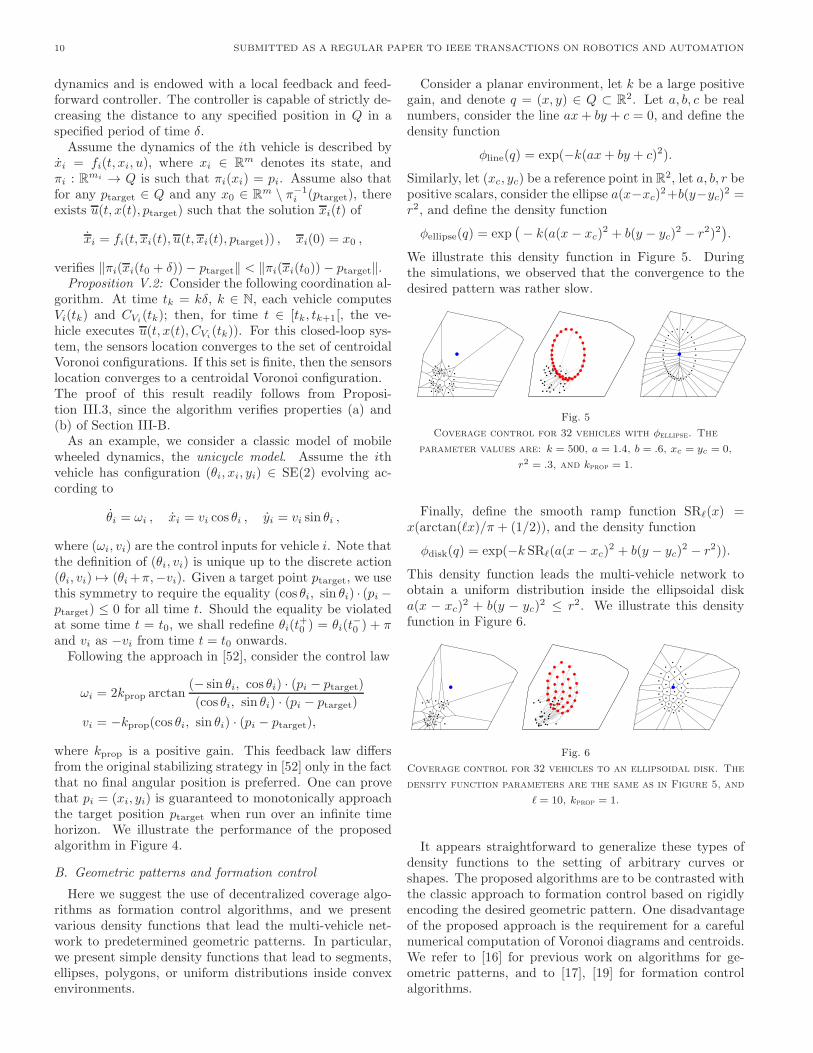
where kprop is a positive gain. This feedback law differsfrom the original stabilizing strategy in [52] only in the factthat no final angular position is preferred. One can provethat pi = (xi, yi) is guaranteed to monotonically approachthe target position ptarget when run over an infinite timehorizon. We illustrate the performance of the proposedalgorithm in Figure 4.

B. Geometric patterns and formation control

Here we suggest the use of decentralized coverage algo-rithms as formation control algorithms, and we presentvarious density functions that lead the multi-vehicle net-work to predetermined geometric patterns. In particular,we present simple density functions that lead to segments,ellipses, polygons, or uniform distributions inside convexenvironments.

Consider a planar environment, let k be a large positivegain, and denote q = (x, y) ∈ Q ⊂ R

2. Let a, b, c be realnumbers, consider the line ax+ by + c = 0, and define thedensity function

φline(q) = exp(−k(ax+ by + c)2).

Similarly, let (xc, yc) be a reference point in R2, let a, b, r be

positive scalars, consider the ellipse a(x−xc)2+b(y−yc)

2 =r2, and define the density function

φellipse(q) = exp(

− k(a(x − xc)2 + b(y − yc)

2 − r2)2)

.

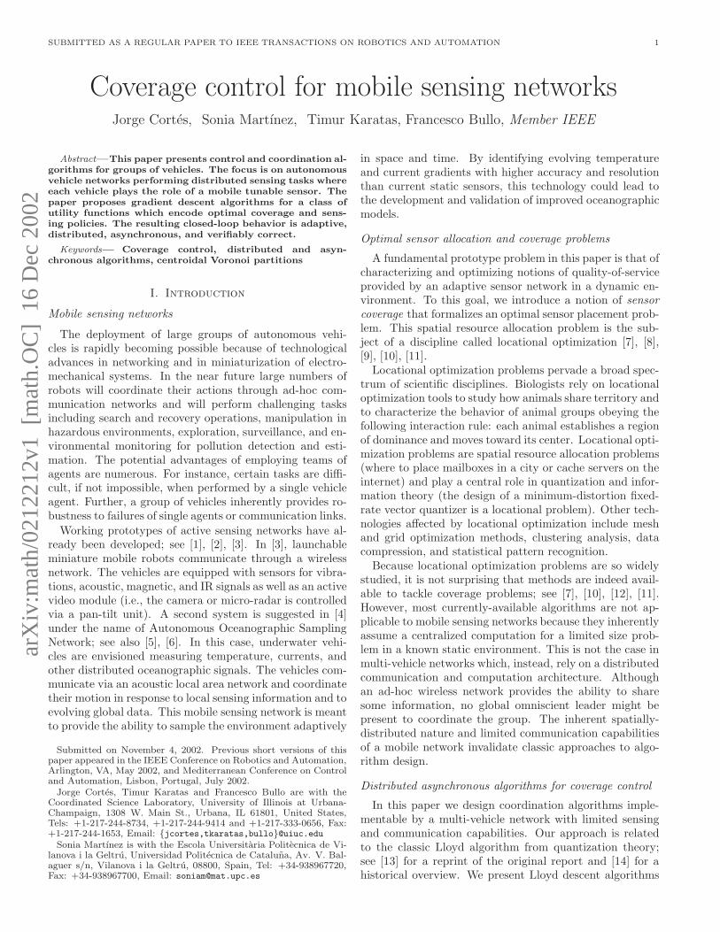
We illustrate this density function in Figure 5. Duringthe simulations, we observed that the convergence to thedesired pattern was rather slow.

Fig. 5

Coverage control for 32 vehicles with φellipse. The

parameter values are: k = 500, a = 1.4, b = .6, xc = yc = 0,

r2 = .3, and kprop = 1.

Finally, define the smooth ramp function SRℓ(x) =x(arctan(ℓx)/π + (1/2)), and the density function

φdisk(q) = exp(−k SRℓ(a(x− xc)2 + b(y − yc)

2 − r2)).

This density function leads the multi-vehicle network toobtain a uniform distribution inside the ellipsoidal diska(x − xc)

2 + b(y − yc)2 ≤ r2. We illustrate this density

function in Figure 6.

Fig. 6

Coverage control for 32 vehicles to an ellipsoidal disk. The

density function parameters are the same as in Figure 5, and

ℓ = 10, kprop = 1.

It appears straightforward to generalize these types ofdensity functions to the setting of arbitrary curves orshapes. The proposed algorithms are to be contrasted withthe classic approach to formation control based on rigidlyencoding the desired geometric pattern. One disadvantageof the proposed approach is the requirement for a carefulnumerical computation of Voronoi diagrams and centroids.We refer to [16] for previous work on algorithms for ge-ometric patterns, and to [17], [19] for formation controlalgorithms.

CORTES, MARTıNEZ, KARATAS AND BULLO: COVERAGE CONTROL FOR MOBILE SENSING NETWORKS 11

Fig. 4

Coverage control for 16 vehicles with mobile wheeled dynamics. The environment and Gaussian density function are as in

Figure 2, and kprop = 3.

VI. Conclusions

We have presented a novel approach to coordination al-gorithms for multi-vehicle networks. The scheme can bethought of as an interaction law between agents and assuch it is implementable in a distributed asynchronousfashion. Numerous extensions appear worth pursuing. Weplan to investigate the setting of non-convex environmentsand non-isotropic sensors. We are currently implementingthese algorithms on a network of all-terrain vehicles. Fur-thermore, we plan to extend the algorithms to provide col-lision avoidance guarantees and to vehicle dynamics whichare not locally controllable.

Acknowledgments

This work was supported by NSF Grant CMS-0100162,ARO Grant DAAD 190110716, and DARPA/AFOSRMURI Award F49620-02-1-0325.

References

[1] C. R. Weisbin, J. Blitch, D. Lavery, E. Krotkov, C. Shoemaker,L. Matthies, and G. Rodriguez, “Miniature robots for space andmilitary missions,” IEEE Robotics & Automation Magazine, vol.6, no. 3, pp. 9–18, 1999.

[2] E. Krotkov and J. Blitch, “The Defense Advanced ResearchProjects Agency (DARPA) tactical mobile robotics program,”International Journal of Robotics Research, vol. 18, no. 7, pp.769–76, 1999.

[3] P. E. Rybski, N. P. Papanikolopoulos, S. A. Stoeter, D. G.Krantz, K. B. Yesin, M. Gini, R. Voyles, D. F. Hougen, B. Nel-son, and M. D. Erickson, “Enlisting rangers and scouts for re-connaissance and surveillance,” IEEE Robotics & AutomationMagazine, vol. 7, no. 4, pp. 14–24, 2000.

[4] T. B. Curtin, J. G. Bellingham, J. Catipovic, and D. Webb,“Autonomous oceanographic sampling networks,” Oceanogra-phy, vol. 6, no. 3, pp. 86–94, 1993.

[5] R. M. Turner and E. H. Turner, “Organization and reorganiza-tion of autonomous oceanographic sampling networks,” in IEEEInt. Conf. on Robotics and Automation, Leuven, Belgium, May1998, pp. 2060–7.

[6] E. Eberbach and S. Phoha, “SAMON: communication, coop-eration and learning of mobile autonomous robotic agents,” inProceedings 11th International Conf. on Tools with ArtificialIntelligence (TAI), Chicago, IL, Nov. 1999, pp. 229–36.

[7] A. Okabe, B. Boots, and K. Sugihara, “Nearest neighbourhoodoperations with generalized Voronoi diagrams: a review,” In-ternational Journal of Geographical Information Systems, vol.8, no. 1, pp. 43–71, 1994.

[8] Z. Drezner, Ed., Facility Location: A Survey of Applicationsand Methods, Springer Series in Operations Research. SpringerVerlag, New York, NY, 1995.

[9] A. Suzuki and A. Okabe, “Using Voronoi diagrams,” In Drezner[8], pp. 103–118.

[10] A. Okabe and A. Suzuki, “Locational optimization problemssolved through Voronoi diagrams,” European Journal of Oper-ational Research, vol. 98, no. 3, pp. 445–56, 1997.

[11] A. Okabe, B. Boots, K. Sugihara, and S. N. Chiu, Spatial Tessel-lations: Concepts and Applications of Voronoi Diagrams, WileySeries in Probability and Statistics. John Wiley & Sons, NewYork, NY, second edition, 2000.

[12] Q. Du, V. Faber, and M. Gunzburger, “Centroidal Voronoitessellations: applications and algorithms,” SIAM Review, vol.41, no. 4, pp. 637–676, 1999.

[13] S. P. Lloyd, “Least squares quantization in PCM,” IEEE Trans-actions on Information Theory, vol. 28, no. 2, pp. 129–137, 1982,Presented as Bell Laboratory Technical Memorandum at a 1957Institute for Mathematical Statistics meeting.

[14] R. M. Gray and D. L. Neuhoff, “Quantization,” IEEE Trans-actions on Information Theory, vol. 44, no. 6, pp. 2325–2383,1998, Commemorative Issue 1948-1998.

[15] H. Yamaguchi and T. Arai, “Distributed and autonomouscontrol method for generating shape of multiple mobile robotgroup,” in IEEE/RSJ Int. Conf. on Intelligent Robots & Sys-tems, Munich, Germany, Sept. 1994, pp. 800–807.

[16] K. Sugihara and I. Suzuki, “Distributed algorithms for formationof geometric patterns with many mobile robots,” Journal ofRobotic Systems, vol. 13, no. 3, pp. 127–39, 1996.

[17] T. Balch and R. Arkin, “Behavior-based formation control formultirobot systems,” IEEE Transactions on Robotics and Au-tomation, vol. 14, no. 6, pp. 926–39, 1998.

[18] M. Egerstedt and X. Hu, “Formation constrained multi-agentcontrol,” IEEE Transactions on Robotics and Automation, vol.17, no. 6, pp. 947–51, 2001.

[19] J. P. Desai, J. P. Ostrowski, and V. Kumar, “Modeling andcontrol of formations of nonholonomic mobile robots,” IEEETransactions on Robotics and Automation, vol. 17, no. 6, pp.905–8, 2001.

[20] P. Tabuada, G. Pappas, and P. Lima, “Feasible formations ofmulti-agent systems,” Automatica, 2002, Submitted.

[21] R. Olfati-Saber and R. M. Murray, “Graph rigidity and dis-tributed formation stabilization of multi-vehicle systems,” inIEEE Conf. on Decision and Control, Las Vegas, NV, 2002, Toappear.

[22] C. Tomlin, G. J. Pappas, and S. S. Sastry, “Conflict resolutionfor air traffic management: a study in multiagent hybrid sys-tems,” IEEE Transactions on Automatic Control, vol. 43, no.4, pp. 509–21, 1998.

[23] E. Frazzoli, Z. H. Mao, J. H. Oh, and E. Feron, “Aircraft conflictresolution via semi-definite programming,” AIAA Journal ofGuidance, Control, and Dynamics, vol. 24, no. 1, pp. 79–86,2001.

12 SUBMITTED AS A REGULAR PAPER TO IEEE TRANSACTIONS ON ROBOTICS AND AUTOMATION

[24] H. Choset, “Coverage for robotics - a survey of recent results,”Annals of Mathematics and Artificial Intelligence, vol. 31, pp.113–126, 2001.

[25] R. Bachmayer and N. Ehrich Leonard, “Vehicle networks forgradient descent in a sampled environment,” in IEEE Conf. onDecision and Control, Dec. 2002, To appear.

[26] A. Jadbabaie, J. Lin, and A. S. Morse, “Coordination of groupsof mobile autonomous agents using nearest neighbor rules,”IEEE Transactions on Automatic Control, July 2002, To ap-pear.

[27] E. Klavins, “Communication complexity of multi-robot sys-tems,” in Workshop on Algorithmic Foundations of Robotics,Nice, France, Dec. 2002, Submitted.

[28] J. Cortes, S. Martınez, T. Karatas, and F. Bullo, “Coveragecontrol for mobile sensing networks,” in IEEE Int. Conf. onRobotics and Automation, Arlington, VA, May 2002, pp. 1327–1332.

[29] J. Cortes, S. Martınez, T. Karatas, and F. Bullo, “Coveragecontrol for mobile sensing networks: variations on a theme,” inMediterranean Conference on Control and Automation, Lisbon,Portugal, July 2002, Electronic proceedings.

[30] R. A. Brooks, “A robust layered control-system for a mobilerobot,” IEEE Journal of Robotics and Automation, vol. 2, no.1, pp. 14–23, 1986.

[31] C. W. Reynolds, “Flocks, herds, and schools: A distributedbehavioral model,” Computer Graphics, vol. 21, no. 4, pp. 25–34, 1987.

[32] R. C. Arkin, Behavior-Based Robotics, Cambridge UniversityPress, New York, NY, 1998.

[33] M. S. Fontan and M. J. Mataric, “Territorial multi-robot taskdivision,” IEEE Transactions on Robotics and Automation, vol.14, no. 5, pp. 815–822, 1998.

[34] A. C. Schultz and L. E. Parker, Eds., Multi-Robot Systems:From Swarms to Intelligent Automata, Washington, DC, June2002. Kluwer Academic Publishers, Proceedings from the 2002NRL Workshop on Multi-Robot Systems.

[35] T. Balch and L. E. Parker, Eds., Robot Teams: From Diversityto Polymorphism, A. K. Peters Ltd., 2002.

[36] L. E. Parker, “Distributed algorithms for multi-robot observa-tion of multiple moving targets,” Autonomous Robots, vol. 12,no. 3, pp. 231–55, 2002.

[37] A. Howard, Maja J. Mataric, and G. S. Sukhatme, “Mobilesensor network deployment using potential fields: A distributedscalable solution to the area coverage problem,” in Proceedingsof the 6th International Conference on Distributed AutonomousRobotic Systems (DARS02), Fukuoka, Japan, 2002, pp. 299–308.

[38] N. A. Lynch, Distributed Algorithms, Morgan Kaufmann Pub-lishers, San Mateo, CA, 1997.

[39] G. Tel, Introduction to Distributed Algorithms, Cambridge Uni-versity Press, New York, NY, second edition, 2001.

[40] J. N. Tsitsiklis, D. P. Bertsekas, and M. Athans, “Distributedasynchronous deterministic and stochastic gradient optimizationalgorithms,” IEEE Transactions on Automatic Control, vol. 31,no. 9, pp. 803–12, 1986.

[41] D. P. Bertsekas and J. N. Tsitsiklis, Parallel and DistributedComputation: Numerical Methods, Athena Scientific, 1997.

[42] S. H. Low and D. E. Lapsey, “Optimization flow control I: Ba-sic algorithm and convergence,” IEEE/ACM Transactions onNetworking, vol. 7, no. 6, pp. 861–74, 1999.

[43] G. Leibon and D. Letscher, “Delaunay triangulations andVoronoi diagrams for Riemannian manifolds,” in Proceedingsof the Sixteenth Annual Symposium on Computational Geome-try (Hong Kong, 2000), New York, 2000, pp. 341–349, ACM.

[44] R. Klein, Concrete and abstract Voronoi diagrams, vol. 400 ofLecture Notes in Computer Science, Springer Verlag, New York,NY, 1989.

[45] A. Suzuki and Z. Drezner, “The p-center location problem in anarea,” Location Science, vol. 4, no. 1/2, pp. 69–82, 1996.

[46] J. Cortes and F. Bullo, “Distributed Lloyd flows for disk coveringand sphere packing problems,” 2002, Preprint.

[47] C. Cattani and A. Paoluzzi, “Boundary integration over linearpolyhedra,” Computer-Aided Design, vol. 22, no. 2, pp. 130–5,1990.

[48] J. Gao, L. J. Guibas, J. Hershberger, Li Zhang, and An Zhu,“Geometric spanner for routing in mobile networks,” in ACMInternational Symposium on Mobile Ad-hoc Networking & Com-puting, Long Beach, CA, Oct. 2001, pp. 45–55.

[49] X.-Y. Li and P.-J. Wan, “Constructing minimum energy mobile

wireless networks,” ACM Journal of Mobile Computing andCommunication Survey, vol. 5, no. 4, 2001.

[50] S. Meguerdichian, S. Slijepcevic, V. Karayan, and M. Potkinjak,“Localized algorithms in wireless ad-hoc networks: Location dis-covery and sensor exposure,” in ACM International Symposiumon Mobile Ad-hoc Networking & Computing, Long Beach, CA,Oct. 2001.

[51] M. Cao and C. Hadjicostis, “Distributed algorithms for Voronoidiagrams and application in ad-hoc networks,” Preprint, Oct.2002.

[52] A. Astolfi, “Exponential stabilization of a wheeled mobile robotvia discontinuous control,” ASME Journal on Dynamic Sys-tems, Measurement, and Control, vol. 121, no. 1, pp. 121–7,1999.

[53] H. K. Khalil, Nonlinear Systems, Prentice Hall, EnglewoodCliffs, NJ, second edition, 1995.

[54] D. G. Luenberger, Linear and Nonlinear Programming,Addison-Wesley, Reading, Massachusetts, second edition, 1984.

VII. Appendix

In this section we collect some relevant facts on descentflows both in the continuous and in the discrete-time set-tings. We do this following [53] and [54], respectively. Weinclude Proposition VII.4 as we are unable to locate it inthe linear and nonlinear programming literature.

Continuous-time descent flows

Consider the differential equation x = X(x), where X :D ⊂ R

N → RN is locally Lipschitz and D is an open

connected set. A set M is said to be (positively) invariantwith respect to X if x(0) ∈ M implies x(t) ∈ M , for allt ∈ R (resp. t ≥ 0). A descent function for X on Ω,V : D → R, is a continuously differentiable function suchthat LXV ≤ 0 on Ω. We denote by E the set of points inΩ where LXV (x) = 0 and by M be the largest invariantset contained in E. Finally, the distance from a point x toa set M is defined as dist(x,M) = infp∈M ‖x− p‖.Lemma VII.1 (LaSalle’s principle) Let Ω ⊂ D be a com-

pact set that it is positively invariant with respect to X .Let x(0) ∈ M and x∗ be an accumulation point of x(t).Then x∗ ∈ M and dist(x(t),M) → 0 as t → ∞.

The following corollary is Exercise 3.22 in [53].

Corollary VII.2: If the set M is a finite collection ofpoints, then the limit of x(t) exists and equals one of them.

Discrete-time descent flows

Let X be a subset of RN . An algorithm T is a continuousmapping from X to X . A set C is said to be positivelyinvariant with respect to T if x0 ∈ C implies T (x0) ∈ C.A point x∗ is said to be a fixed point of T if T (x∗) = x∗.We denote the set of fixed points of T by Γ. A descentfunction for T on C, Z : X → R+, is any nonnegative real-valued continuous function satisfying Z(T (x)) ≤ Z(x) forx ∈ C, where the inequality is strict if x 6∈ Γ. Typically,Z is the objective function to be minimized, and T reflectsthis goal by yielding a point that reduces (or at least doesnot increase) Z.

Lemma VII.3 (Global convergence theorem) Let C ⊂X be a compact set that it is positively invariant with re-spect to T . Let x0 ∈ C and denote xm = T (xm−1), m ≥ 1.Let x∗ be an accumulation point of the sequence xmm≥1.

CORTES, MARTıNEZ, KARATAS AND BULLO: COVERAGE CONTROL FOR MOBILE SENSING NETWORKS 13

Then x∗ ∈ Γ, dist(xm,Γ) → 0 and Z(xm) → Z(x∗) asm → ∞.Proposition VII.4: If the set Γ is a finite collection of

points, then xm converges and equals one of them.Proof: Let x∗ be an accumulation point of xm

and assume the whole sequence does not converge to it.Then, there exists an ǫ > 0 such that for all m0, thereis a m′ > m0 such that ‖xm′ − x∗‖ > ǫ. Let d be theminimum of all the distances between the points in Γ. Fixǫ′ = mind/2, ǫ. Since T is continuous and Γ is finite,there exists δ > 0 such that ‖x − z‖ < δ, with z ∈ Γ,implies ‖T (x) − z‖ < ǫ′ (that is, for each z ∈ Γ, thereexists such δ(z), and we take the minimum over Γ).Now, since dist(xm,Γ) → 0, there exists m1 such that for

all m ≥ m1, dist(xm,Γ) < δ. Also, we know that there is asubsequence of xm which converges to x∗, let us denoteit by xmk

k≥1. For δ, there exists mk1such that for all

k ≥ k1, we have ‖xmk− x∗‖ < δ.

Let m0 = maxm1,mk1. Take k such that mk ≥ m0

Then,

‖xmk+1 − x∗‖ = ‖T (xmk)− x∗‖ < ǫ′ . (13)

Now we are going to prove that ‖xmk+1 − x∗‖ < δ. Ifd/2 ≤ δ, then this claim is straightforward, since ǫ′ ≤ d/2.If d/2 > δ, suppose that ‖xmk+1−x∗‖ > δ. Since mk+1 >m0 ≥ m1, then dist(xmk+1,Γ) < δ. Therefore, there existsy ∈ Γ such that ‖xmk+1 − y‖ < δ. Necessarily, y 6= x∗.Now, by the triangle inequality, ‖x− y‖ ≤ ‖x− xmk+1‖ +‖xmk+1 − y‖. Then,

‖xmk+1 − x∗‖ ≥ ‖x− y‖ − ‖xmk+1− y‖ ≥ d− δ > d/2 ,

which contradicts (13). Therefore, ‖xmk+1−x∗‖ < δ. Thisargument can be iterated to prove that for all m ≥ m0, wehave ‖xm − x∗‖ < δ. Let us take now m′ > m0 such that‖xm′−x∗‖ > ǫ. Since m′−1 ≥ m0, we have ‖xm′−1−x∗‖ <δ, and therefore

‖xm′ − x∗‖ = ‖T (xm′−1)− x∗‖ < ǫ′ ≤ ǫ ,

which is a contradiction. Therefore, xm converges to x∗.