Submesoscale dispersion in the vicinity of theDeepwater Horizon spillAndrew C. Pojea, Tamay M. Özgökmenb,1, Bruce L. Lipphardt, Jr.c, Brian K. Hausb, Edward H. Ryanb, Angelique C. Hazab,Gregg A. Jacobsd, A. J. H. M. Reniersb, Maria Josefina Olascoagab, Guillaume Novellib, Annalisa Griffae,Francisco J. Beron-Verab, Shuyi S. Chenb, Emanuel Coelhod, Patrick J. Hogand, Albert D. Kirwan, Jr.c, Helga S. Huntleyc,and Arthur J. Marianob

aDepartment of Mathematics, Graduate Physics Program, College of Staten Island, City University of New York, New York, NY 10314; bDepartment of OceanSciences, Rosenstiel School of Marine and Atmospheric Sciences, University of Miami, Miami, FL 33176; cSchool of Marine Science and Policy, University ofDelaware, Newark, DE 19716; dOcean Dynamics and Prediction, Naval Research Laboratory, Stennis Space Center, Hancock County, MS 39529; and eIstituto diScienze Marine, Consiglio Nazionale delle Ricerche, 19032 La Spezia, Italy

Edited by Carl Wunsch, Harvard University, Cambridge, MA, and approved July 24, 2014 (received for review February 7, 2014)

Reliable forecasts for the dispersion of oceanic contamination areimportant for coastal ecosystems, society, and the economy asevidenced by the Deepwater Horizon oil spill in the Gulf of Mexicoin 2010 and the Fukushima nuclear plant incident in the PacificOcean in 2011. Accurate prediction of pollutant pathways andconcentrations at the ocean surface requires understanding oceandynamics over a broad range of spatial scales. Fundamental ques-tions concerning the structure of the velocity field at the subme-soscales (100 m to tens of kilometers, hours to days) remainunresolved due to a lack of synoptic measurements at these scales.Using high-frequency position data provided by the near-simulta-neous release of hundreds of accurately tracked surface drifters,we study the structure of submesoscale surface velocity fluctua-tions in the Northern Gulf of Mexico. Observed two-point statisticsconfirm the accuracy of classic turbulence scaling laws at 200-m to50-km scales and clearly indicate that dispersion at the submeso-scales is local, driven predominantly by energetic submesoscalefluctuations. The results demonstrate the feasibility and utility ofdeploying large clusters of drifting instruments to provide synop-tic observations of spatial variability of the ocean surface velocityfield. Our findings allow quantification of the submesoscale-drivendispersion missing in current operational circulation models andsatellite altimeter-derived velocity fields.

ocean dispersion | pollutant patterns | geophysical turbulence |Lagrangian transport

The Deepwater Horizon (DwH) incident was the largest acci-dental oil spill into marine waters in history with some 4.4

million barrels released into the DeSoto Canyon of the northernGulf of Mexico (GoM) from a subsurface pipe over ∼84 d in thespring and summer of 2010 (1). Primary scientific questions, withimmediate practical implications, arising from such catastrophicpollutant injection events are the path, speed, and spreading rateof the pollutant patch. Accurate prediction requires knowledge ofthe ocean flow field at all relevant temporal and spatial scales.Whereas ocean general circulation models were widely used duringand after the DwH incident (2–6), such models only capture themain mesoscale processes (spatial scale larger than 10 km) in theGoM. The main factors controlling surface dispersion in theDeSoto Canyon region remain unclear. The region lies betweenthe mesoscale eddy-driven deep water GoM (7) and the wind-driven shelf (8) while also being subject to the buoyancy input ofthe Mississippi River plume during the spring and summer months(9). Images provided by the large amounts of surface oil producedin the DwH incident revealed a rich array of flow patterns (10)showing organization of surface oil not only by mesoscale straininginto the loop current “Eddy Franklin,” but also by submesoscaleprocesses. Such processes operate at spatial scales and involvephysics not currently captured in operational circulation models.Submesoscale motions, where they exist, can directly influence the

local transport of biogeochemical tracers (11, 12) and providepathways for energy transfer from the wind-forced mesoscales tothe dissipative microscales (13–15). Dynamics at the submesoscaleshave been the subject of recent research (16–20). However, theinvestigation of their effect on ocean transport has been pre-dominantly modeling based (13, 21–23) and synoptic observations,at adequate spatial and temporal resolutions, are rare (24, 25). Themechanisms responsible for the establishment, maintenance, andenergetics of such features in the Gulf of Mexico remain unclear.Instantaneous measurement of all representative spatiotem-

poral scales of the ocean state is notoriously difficult (26). Aspreviously reviewed (27), traditional observing systems are notideal for synoptic sampling of near-surface flows at the sub-mesoscale. Owing to the large spacing between ground tracks(28) and along-track signal contamination from high-frequencymotions (29), gridded altimeter-derived sea level anomalies onlyresolve the largest submesoscale motions. Long time-series ship-track current measurements attain similar, larger than 2 km,spatial resolutions, and require averaging the observations overevolving ocean states (30). Simultaneous, two-point accousticDoppler current profiler measurements from pairs of ships (25)provide sufficient resolution to show the existence of energeticsubmesoscale fluctuations in the mixed layer, but do not ex-plicitly quantify the scale-dependent transport induced by suchmotions at the surface. Lagrangian experiments, centered ontracking large numbers of water-following instruments, providethe most feasible means of obtaining spatially distributed,

Significance

We report here on results obtained from the largest upper-ocean dispersion field program conducted to date. The obser-vations provided, for the first time to our knowledge, an ac-curate and nearly simultaneous description of the ocean surfacevelocity field on spatial scales ranging from 100 m to 100 km.We show conclusively that ocean flows contain significant energyat scales below 10 km and that their fluctuations dictate the initialspread of tracer/pollutant clouds. Neither state-of-the art opera-tional models nor satellite altimeters capture the flows neededfor accurately estimating the dispersion of surface particles.

Author contributions: A.C.P., T.M.Ö., B.K.H., E.H.R., A.C.H., G.A.J., A.G., S.S.C., A.D.K., andH.S.H. designed research; A.C.P., T.M.Ö., B.L.L., B.K.H., E.H.R., G.A.J., A.J.H.M.R., M.J.O.,G.N., S.S.C., E.C., and P.J.H. performed research; A.C.P., T.M.Ö., B.L.L., B.K.H., A.C.H., G.A.J.,G.N., A.G., F.J.B.-V., E.C., A.D.K., and A.J.M. contributed new reagents/analytic tools; A.C.P.,T.M.Ö., B.L.L., E.H.R., A.C.H., G.A.J., A.J.H.M.R., M.J.O., F.J.B.-V., and E.C. analyzed data;and A.C.P. and T.M.Ö. wrote the paper.

The authors declare no conflict of interest.

This article is a PNAS Direct Submission.

Freely available online through the PNAS open access option.1To whom correspondence should be addressed. Email: tozgokmen@gmail.com.

www.pnas.org/cgi/doi/10.1073/pnas.1402452111 PNAS | September 2, 2014 | vol. 111 | no. 35 | 12693–12698

ENVIRONMEN

TAL

SCIENCE

S

simultaneous measurements of the structure of the ocean’s sur-face velocity field on 100-m to 10-km length scales.Denoting a trajectory by x(a, t), where x(a, t0) = a, the relative

separation of a particle pair is given by Dðt;D0Þ= xða1; tÞ−xða2; tÞ=D0 +

R tt0Δvðt′;D0Þdt′, where the Lagrangian velocity

difference is defined by Δv(t, D0) = v(a1, t) − v(a2, t). The sta-tistical quantities of interest, both practically and theoretically,are the scale-dependent relative dispersion D2(t) = ⟨D · D⟩ (av-eraged over particle pairs) and the average longitudinal or sep-aration velocity, Δv(r), at a given separation, r. The velocity scaleis defined by the second order structure function ΔvðrÞ=

ffiffiffiffiffiffiffiffiffiffihδv2i

p,

where δv(r) = (v(x + r) − v(x)) · r/krk (31, 32) where the aver-aging is now conditioned on the pair separation r.The applicability of classical dispersion theories (32–34) de-

veloped in the context of homogeneous, isotropic turbulence withlocalized spectral forcing, to ocean flows subject to the effects ofrotation, stratification, and complex forcing at disparate length andtime scales remains unresolved. Turbulence theories broadly pre-dict two distinct dispersion regimes depending upon the shape ofthe spatial kinetic energy spectrum, E(k) ∼ k−β, of the velocity field(35). For sufficiently steep spectra (β ≥ 3) the dispersion is expectedto grow exponentially, D ∼ eλt with a scale-independent rate. At thesubmesoscales (∼ 100 m–10 km), this nonlocal growth rate will thenbe determined by the mesoscale motions currently resolved bypredictive models. For shallower spectra (1 < β < 3), however, thedispersion is local, D ∼ t2/(3−β), and the growth rate of a pollutantpatch is dominated by advective processes at the scale of the patch.Accurate prediction of dispersion in this regime requires resolutionof the advecting field at smaller scales than the mesoscale.Whereas compilations of data from dye measurements broadly

support local dispersion in natural flows (36), the range of scales inany particular dye experiment is limited. A number of Lagrangian

observational studies have attempted to fill this gap. LaCasce andOhlmann (37) considered 140 pairs of surface drifters on the GoMshelf over a 5-y period and found evidence of a nonlocal regimefor temporally smoothed data at 1-km scales. Koszalka et al. (38)using O(100) drifter pairs with D0 < 2 km launched over 18 mo inthe Norwegian Sea, found an exponential fit for D2(t) for a limitedtime (t = 0.5 − 2 d), although the observed longitudinal velocitystructure function is less clearly fit by a corresponding quadratic.They concluded that a nonlocal dispersion regime could not beidentified. In contrast, Lumpkin and Elipot (39) found evidence oflocal dispersion at 1-km scales using 15-m drogued drifterslaunched in the winter-time North Atlantic. It is not clear how theaccuracy of the Argos positioning system (150–1,000 m) used inthese studies affects the submesoscale dispersion estimates.Schroeder et al. (40), specifically targeting a coastal front usinga multiscale sampling pattern, obtained results consistent withlocal dispersion, but the statistical significance (maximum 64pairs) remained too low to be definitive.

ResultsThe primary goal of the Grand Lagrangian Deployment (GLAD)experiment was to quantify the scale dependence of the surface-velocity field from synoptic observations of two-point Lagrangianposition and velocity increments by simultaneously deploying anunprecedented number of drifters. The critical program design el-ement was the use of ∼300 GPS-equipped Coastal Ocean DynamicsExperiment (CODE) drifters (41) to provide sufficient sampling formeasuring two-point Lagrangian velocity and displacement statis-tics. CODE drifters, with submerged sails ∼1 m deep by 1 m wide,are designed and tested to follow upper-ocean flows in the presenceof wind and waves. All GLAD drifters were launched during theperiod of July 20 to July 31, 2012; during the same season as the

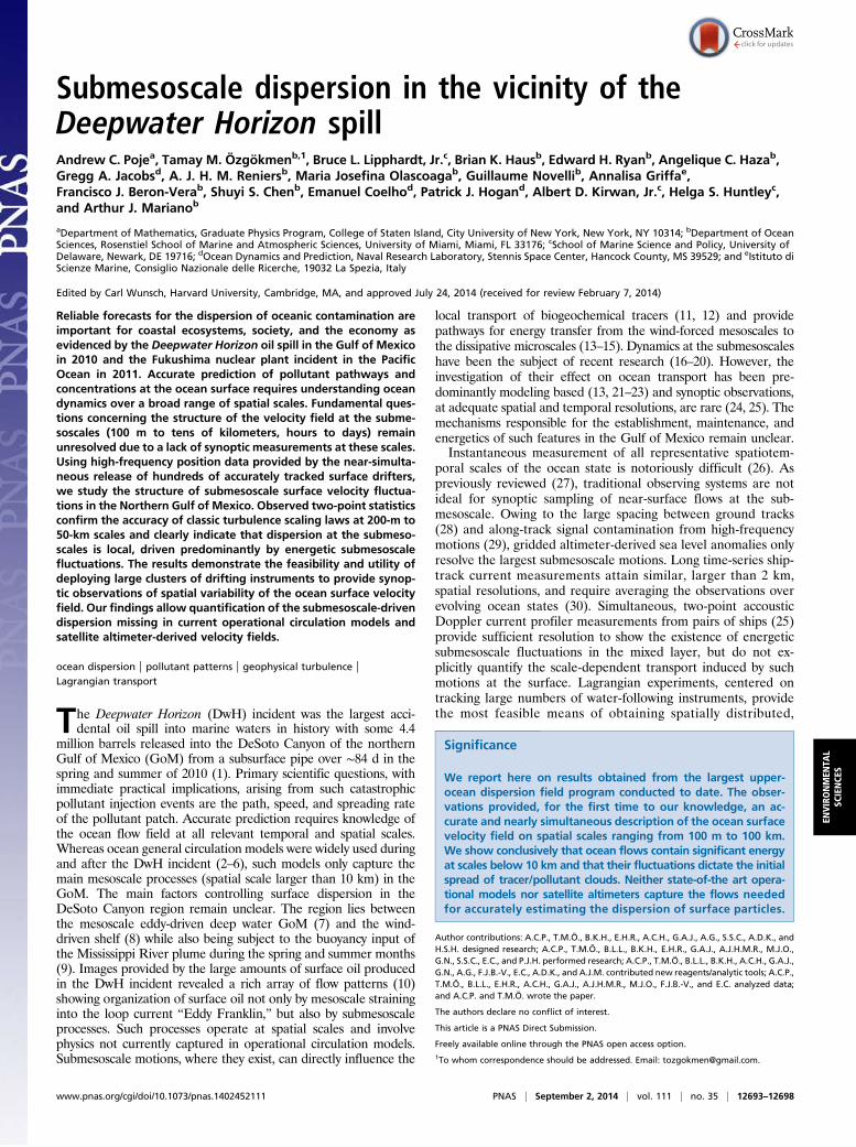
Fig. 1. Multiscale flows near the DwH and DeSoto Canyon region. (A) Synthetic aperture radar (SAR) image of the DwH oil slick taken on May 17, 2010. The reddiamond marks the location of the DwH wellhead, and the Inset shows the geographic location. (B) Drifter launch patterns: The actual pattern obtained (redcircles) for S1 at the launch time of the last drifter compared with the targeted template (black circles). The Inset shows a single node of the multiscale launchpattern. (C) Chlorophyll-a concentration (indicative of phytoplankton suspended in the upper ocean flows) derived from the moderate resolution imagingspectroradiometer sensor aboard theAqua satellite on July 12, 2012. The similarity of this image toA indicates that the GLAD experiment sampled flow conditionssimilar to those during the spill. (D) The time evolution of the number of drifter pairs at given separation distances for the S2 release (pair numbers on log scale).

12694 | www.pnas.org/cgi/doi/10.1073/pnas.1402452111 Poje et al.

DwH event 2 y earlier. A satellite sea-surface color image taken 8d before the first GLAD drifter launch shows striking similarities tosatellite images during the DwH event (Fig. 1 A and C).To obtain high densities of multipoint, contemporaneous po-

sition and velocity data at a range of separation scales spanningthe meso–submesoscale boundary, drifters were released in aspace-filling S configuration within an area ∼8 km × 10 km. Theconfiguration provides synoptic sampling at the upper boundary ofthe submesoscale range while minimizing the time to execute thedeployment with a single ship. The S track consists of 10 nodesspaced at 2 km with each node containing nine drifters arranged intriplets of nested equilateral triangles, with separations of 100 mbetween drifters within a triplet and of 500 m between tripletswithin a node (Fig. 1B). The pattern allows simultaneous samplingof multiple separation scales between 100 m and 10 km. The typicalduration for the release of all 90 drifters was approximately 5 h. Theevolution of the number of particle pairs at given separation dis-tances (Fig. 1D) indicates that large numbers of simultaneousdrifter pairs, especially at submesoscale separations, were obtained.Initial 21-d trajectories for three drifter clusters launched within

the DeSoto Canyon, S1 (near the DwH site, 89 drifters), S2

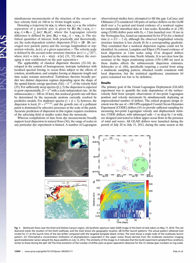
(central DeSoto Canyon targeting a surface salinity front, 90drifters), and T 1 (northern tip of DeSoto Canyon, 27 drifters) areshown in Fig. 2. The degree of confinement of surface waterwithin the canyon and the role played by observed surface densityfronts are quantified by drifter residence time statistics. Trajec-tories in Fig. 2 are coded by residence time, defined as the totalamount of time spent within the closed region bounded by the1,000-m isobath and the 28.1°N latitude line over the 28-d periodafter launch. The residence time for all drifters in the S1 and T 1deployments is longer than 1 wk with a large number of S1 driftersremaining within the canyon for more than 1 mo. Residence timesfor drifters in the S2 launch, specifically those targeting a frontalfeature in surface density, show much larger variation.Surface salinity measurements (Fig. 3) reveal a highly foliated

horizontal-density structure associated with the variability in theMississippi River outflow (MRO) plume. Residence times inboth S launches are extremely sensitive to launch location andare strongly correlated with initial salinity. This is especially truefor the S2 launch where drifters launched on the more salineeastern side of the front rapidly exit the canyon, whereas those

Fig. 2. GLAD trajectories. Trajectories for S1 and T 1 (Upper) and S2(Lower) with initial and day-21 positions marked by symbols. Trajectories arecolor coded based on total residence time, τ, in the canyon: red triangles forτ < 7 d, gold circles for 7 < τ < 14 d, green circles for 14 < τ < 21 d, and bluesquares for τ > 21 d. The zonal line at 28.1°N marks the latitude used asboundary for residence time estimates inside the canyon.

Fig. 3. Sensitivity to launch positions. Initial launch locations and ship-tracksea-surface salinity maps for S1 (Upper) and S2 (Lower) launches. Initialconditions are color coded based on total residence time in the canyon.Refer to Fig. 2 legend for the description of color coding. The colored tracksand the color bar indicate sea surface salinity measured along ship track.

Poje et al. PNAS | September 2, 2014 | vol. 111 | no. 35 | 12695

ENVIRONMEN

TAL

SCIENCE

S

launched in less saline water remain within the western canyonfor considerably longer times.Spatial and temporal distributions of basic dispersion statistics

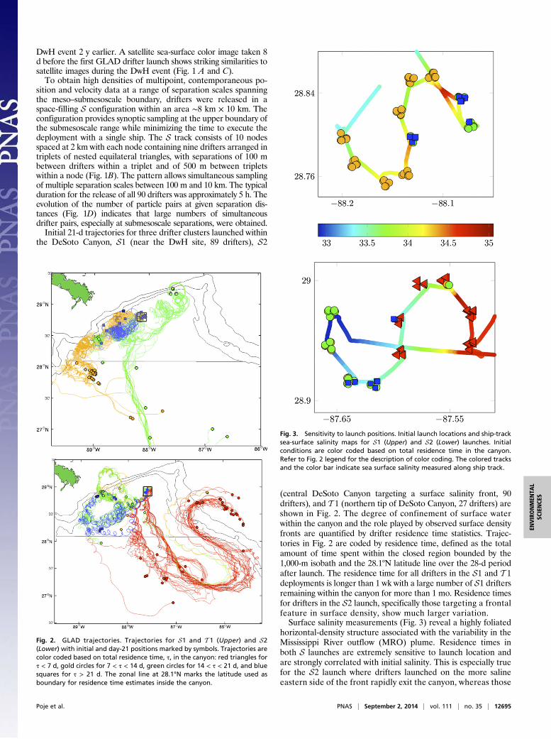
for four drifter groups are shown in Fig. 4. The S2 launch hasbeen split into two groups based on residence time and surfacesalinity characteristics: drifters launched in low surface salinitywater with residence times greater than 7 d (referred to as MROdrifters) and those launched in higher surface salinity water withshort residence times. Center of mass trajectories for each group(symbol marking every 3 d) as well as dispersion ellipses in-dicating the size and orientation of the SD of the relative dis-persion of drifters about the cluster center of mass are plotted.Observations confirm the disparity between slow, isotropic dis-persion inside the canyon and rapid stretching outside.The top panels in Fig. 5 show relative dispersion curves [here

D(t)] for S1 and S2 conditioned on the initial separation distanceof drifter pairs. Initial separation bins are centered at 0.1, 0.5, 5,and 10 km. Data densities range from 48 drifter pairs for the0.1-km S1 bin to 1,034 pairs for the 10-km S1 bin. Error bars,shown for the smallest initial separations in S1, were computedfrom standard 95% confidence intervals produced by 2,000 boot-strapped samples at each time. Both launches indicate that initialgrowth depends strongly on the initial separation scale withfaster growth rates for smaller separations. In the S1 launch,which was entirely confined to the canyon for 1 wk, dispersionfrom initial scales below 1 km is arrested at ∼8-km length scales,whereas dispersion from initial scales above 1 km shows arrest at∼30-km length scales. All curves indicate considerable energy atnear-inertial frequencies. Similar behavior is observed in the S2data for the smallest separation scale. Corresponding dispersioncurves derived from artificial drifters (launched at the sameinitial time and position as the GLAD drifters) advected by thegeostrophic velocity field derived from AVISO gridded altimeterdata do not exhibit this pattern. Neither relative nor absolutedispersion metrics for any of the drifter launches exhibited as-ymptotic behavior 28 d after release.Scale-dependent dispersion results are displayed in Fig. 5, Bot-

tom, where, for all three clusters, the dispersion rate given by thetime-scale λ(r) = Δv(r)/r scales with r−β, β ≠ 0 for separation scalesbelow 10 km. The observed exponent in each case is consistent

with Richardson’s two-thirds law and a local dispersion regimewhere the underlying Eulerian kinetic energy spectrum scales areconsiderably shallower than the E(k) ∼ k−3 spectrum expected inan enstrophy cascading regime. Comparison of dispersion rates forsynthetic drifters launched at identical locations and times to thosein S1 and S2, and advected by a data-assimilating, operationalmodel (Navy Coastal Ocean Model, NCOM) simulation of the gulfshow reasonable agreement with data at mesoscales (r > 10 km),but poor agreement at submesoscales where the model fieldsnecessarily impose steep spectral decay near the model gridspacing. In contrast to the situation where small-scale dispersion isdominated by the strain of large scale, nearly 2D ocean flows, theobservations clearly indicate the presence of energetic, local

Fig. 4. Dispersion ellipses. Trajectories and dispersion ellipses for S1 (blue)and T 1 (yellow). Launch S2 has been separated into two groups: driftersinitialized in MRO water with residence times in the canyon longer than 7 d(red) and those with residence times in the canyon less than 7 d (green).

Fig. 5. Dispersion diagrams from GLAD in comparison with NCOM andAVISO. Time dependence of the relative dispersion, D(t), for four differentinitial separation distances for the S1 (Top) and S2 (Middle) launches. Forcomparison, data from identical launches advected using geostrophic ve-locities produced by AVISO altimeter data are shown in red. (Bottom) Thescale-dependent pair separation rate as function of separation distance forthe three launches (S1, S2, and T 1) shown in solid symbols with corre-sponding model results from a 3-km resolution NCOM simulation for S1 and S2shown in open symbols. The slope indicates the Richardson regime, Δv/r ∼ r−2/3.

12696 | www.pnas.org/cgi/doi/10.1073/pnas.1402452111 Poje et al.

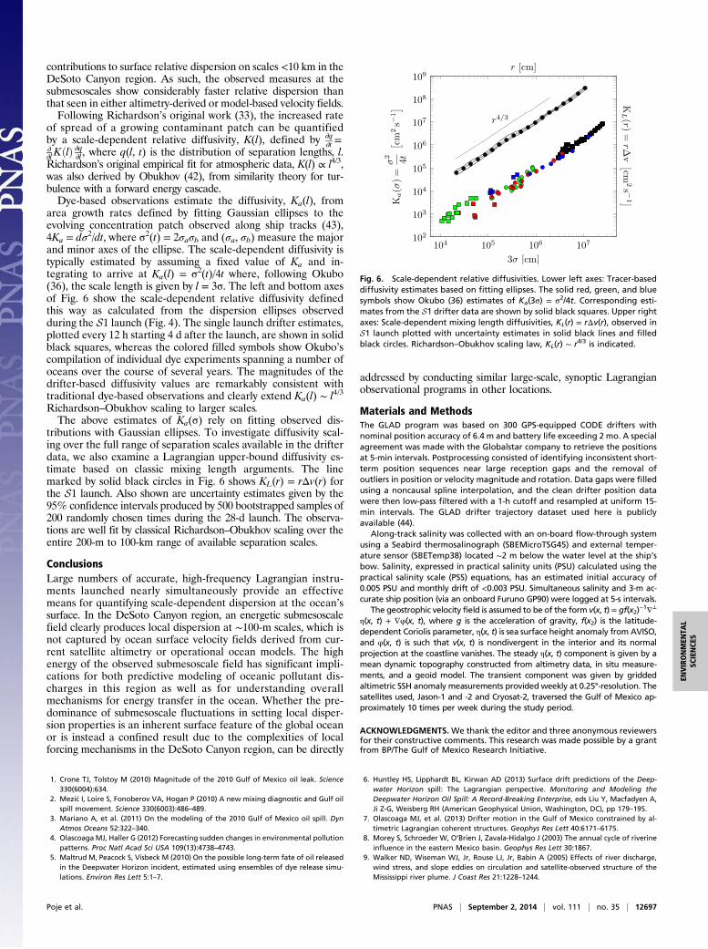
contributions to surface relative dispersion on scales <10 km in theDeSoto Canyon region. As such, the observed measures at thesubmesoscales show considerably faster relative dispersion thanthat seen in either altimetry-derived or model-based velocity fields.Following Richardson’s original work (33), the increased rate

of spread of a growing contaminant patch can be quantifiedby a scale-dependent relative diffusivity, K(l), defined by ∂q

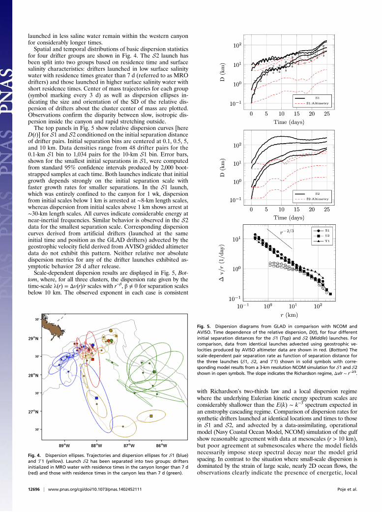
∂t =∂∂l KðlÞ ∂q∂l , where q(l, t) is the distribution of separation lengths, l.Richardson’s original empirical fit for atmospheric data, K(l) ∝ l4/3,was also derived by Obukhov (42), from similarity theory for tur-bulence with a forward energy cascade.Dye-based observations estimate the diffusivity, Ka(l), from

area growth rates defined by fitting Gaussian ellipses to theevolving concentration patch observed along ship tracks (43),4Ka = dσ2/dt, where σ2(t) = 2σaσb and (σa, σb) measure the majorand minor axes of the ellipse. The scale-dependent diffusivity istypically estimated by assuming a fixed value of Ka and in-tegrating to arrive at Ka(l) = σ2(t)/4t where, following Okubo(36), the scale length is given by l = 3σ. The left and bottom axesof Fig. 6 show the scale-dependent relative diffusivity definedthis way as calculated from the dispersion ellipses observedduring the S1 launch (Fig. 4). The single launch drifter estimates,plotted every 12 h starting 4 d after the launch, are shown in solidblack squares, whereas the colored filled symbols show Okubo’scompilation of individual dye experiments spanning a number ofoceans over the course of several years. The magnitudes of thedrifter-based diffusivity values are remarkably consistent withtraditional dye-based observations and clearly extend Ka(l) ∼ l4/3

Richardson–Obukhov scaling to larger scales.The above estimates of Ka(σ) rely on fitting observed dis-

tributions with Gaussian ellipses. To investigate diffusivity scal-ing over the full range of separation scales available in the drifterdata, we also examine a Lagrangian upper-bound diffusivity es-timate based on classic mixing length arguments. The linemarked by solid black circles in Fig. 6 shows KL(r) = rΔv(r) forthe S1 launch. Also shown are uncertainty estimates given by the95% confidence intervals produced by 500 bootstrapped samples of200 randomly chosen times during the 28-d launch. The observa-tions are well fit by classical Richardson–Obukhov scaling over theentire 200-m to 100-km range of available separation scales.

ConclusionsLarge numbers of accurate, high-frequency Lagrangian instru-ments launched nearly simultaneously provide an effectivemeans for quantifying scale-dependent dispersion at the ocean’ssurface. In the DeSoto Canyon region, an energetic submesoscalefield clearly produces local dispersion at ∼100-m scales, which isnot captured by ocean surface velocity fields derived from cur-rent satellite altimetry or operational ocean models. The highenergy of the observed submesoscale field has significant impli-cations for both predictive modeling of oceanic pollutant dis-charges in this region as well as for understanding overallmechanisms for energy transfer in the ocean. Whether the pre-dominance of submesoscale fluctuations in setting local disper-sion properties is an inherent surface feature of the global oceanor is instead a confined result due to the complexities of localforcing mechanisms in the DeSoto Canyon region, can be directly

addressed by conducting similar large-scale, synoptic Lagrangianobservational programs in other locations.

Materials and MethodsThe GLAD program was based on 300 GPS-equipped CODE drifters withnominal position accuracy of 6.4 m and battery life exceeding 2 mo. A specialagreement was made with the Globalstar company to retrieve the positionsat 5-min intervals. Postprocessing consisted of identifying inconsistent short-term position sequences near large reception gaps and the removal ofoutliers in position or velocity magnitude and rotation. Data gaps were filledusing a noncausal spline interpolation, and the clean drifter position datawere then low-pass filtered with a 1-h cutoff and resampled at uniform 15-min intervals. The GLAD drifter trajectory dataset used here is publiclyavailable (44).

Along-track salinity was collected with an on-board flow-through systemusing a Seabird thermosalinograph (SBEMicroTSG45) and external temper-ature sensor (SBETemp38) located ∼2 m below the water level at the ship’sbow. Salinity, expressed in practical salinity units (PSU) calculated using thepractical salinity scale (PSS) equations, has an estimated initial accuracy of0.005 PSU and monthly drift of <0.003 PSU. Simultaneous salinity and 3-m ac-curate ship position (via an onboard Furuno GP90) were logged at 5-s intervals.

The geostrophic velocity field is assumed to be of the form v(x, t)= gf(x2)−1∇⊥

η(x, t) + ∇φ(x, t), where g is the acceleration of gravity, f(x2) is the latitude-dependent Coriolis parameter, η(x, t) is sea surface height anomaly from AVISO,and φ(x, t) is such that v(x, t) is nondivergent in the interior and its normalprojection at the coastline vanishes. The steady η(x, t) component is given by amean dynamic topography constructed from altimetry data, in situ measure-ments, and a geoid model. The transient component was given by griddedaltimetric SSH anomaly measurements provided weekly at 0.25°-resolution. Thesatellites used, Jason-1 and -2 and Cryosat-2, traversed the Gulf of Mexico ap-proximately 10 times per week during the study period.

ACKNOWLEDGMENTS. We thank the editor and three anonymous reviewersfor their constructive comments. This research was made possible by a grantfrom BP/The Gulf of Mexico Research Initiative.

1. Crone TJ, Tolstoy M (2010) Magnitude of the 2010 Gulf of Mexico oil leak. Science330(6004):634.

2. Mezi�c I, Loire S, Fonoberov VA, Hogan P (2010) A new mixing diagnostic and Gulf oilspill movement. Science 330(6003):486–489.

3. Mariano A, et al. (2011) On the modeling of the 2010 Gulf of Mexico oil spill. DynAtmos Oceans 52:322–340.

4. OlascoagaMJ, Haller G (2012) Forecasting sudden changes in environmental pollutionpatterns. Proc Natl Acad Sci USA 109(13):4738–4743.

5. Maltrud M, Peacock S, Visbeck M (2010) On the possible long-term fate of oil releasedin the Deepwater Horizon incident, estimated using ensembles of dye release simu-lations. Environ Res Lett 5:1–7.

6. Huntley HS, Lipphardt BL, Kirwan AD (2013) Surface drift predictions of the Deep-water Horizon spill: The Lagrangian perspective. Monitoring and Modeling theDeepwater Horizon Oil Spill: A Record-Breaking Enterprise, eds Liu Y, Macfadyen A,Ji Z-G, Weisberg RH (American Geophysical Union, Washington, DC), pp 179–195.

7. Olascoaga MJ, et al. (2013) Drifter motion in the Gulf of Mexico constrained by al-timetric Lagrangian coherent structures. Geophys Res Lett 40:6171–6175.

8. Morey S, Schroeder W, O’Brien J, Zavala-Hidalgo J (2003) The annual cycle of riverineinfluence in the eastern Mexico basin. Geophys Res Lett 30:1867.

9. Walker ND, Wiseman WJ, Jr, Rouse LJ, Jr, Babin A (2005) Effects of river discharge,wind stress, and slope eddies on circulation and satellite-observed structure of theMississippi river plume. J Coast Res 21:1228–1244.

Fig. 6. Scale-dependent relative diffusivities. Lower left axes: Tracer-baseddiffusivity estimates based on fitting ellipses. The solid red, green, and bluesymbols show Okubo (36) estimates of Ka(3σ) = σ2/4t. Corresponding esti-mates from the S1 drifter data are shown by solid black squares. Upper rightaxes: Scale-dependent mixing length diffusivities, KL(r) = rΔv(r), observed inS1 launch plotted with uncertainty estimates in solid black lines and filledblack circles. Richardson–Obukhov scaling law, KL(r) ∼ r4/3 is indicated.

Poje et al. PNAS | September 2, 2014 | vol. 111 | no. 35 | 12697

ENVIRONMEN

TAL

SCIENCE

S

10. Jones CE, Minchew B, Holt B, Hensley S (2011) Studies of the Deepwater Horizon oilspill with the UAVSAR radar. Monitoring and Modeling the Deepwater Horizon OilSpill: A Record-Breaking Enterprise, eds Liu Y, Macfadyen A, Ji Z-G, Weisberg RH(American Geophysical Union, Washington, DC), pp 33–50.

11. Klein P, Lapeyre G (2009) The oceanic vertical pump induced by mesoscale and sub-mesoscale turbulence. Annu Rev Mar Sci 1:351–375.

12. Levy M, Ferrari R, Franks P, Martin A, Riviere P (2012) Bringing physics to life at thesubmesoscale. Geophys Res Lett 39:L14602.

13. McWilliams J (2008) Fluid dynamics at the margin of rotational control. Environ FluidMech 8:441–449.

14. Fox-Kemper B, et al. (2011) Parameterization of mixed-layer eddies: III. Implementationand impact in global ocean climate simulations. Ocean Model 39:61–78.

15. Nikurashin M, Vallis GK, Adcroft A (2013) Routes to energy dissipation for geostrophicflows in the Southern Ocean. Nat Geosci 6:48–51.

16. Müller P, McWilliams J, Molemaker M (2005) Routes to dissipation in the ocean: Thetwo-dimensional/three-dimensional turbulence conundrum. Marine Turbulence:Theories, Observations, and Models. Results of the CARTUM Project, eds Baumert HZ,Simpson J, Sündermann J (Cambridge Univ Press, Cambridge, UK), pp 397–405.

17. Capet X, McWilliams J, Molemaker M, Shchepetkin A (2008) Mesoscale to sub-mesoscale transition in the California Current System: I flow structure, eddy flux andobservational tests. J Phys Oceanogr 38:29–43.

18. Fox-Kemper B, Ferrari R, Hallberg R (2008) Parameterization of mixed-layer eddies.Part I: Theory and diagnosis. J Phys Oceanogr 38:1145–1165.

19. Taylor J, Ferrari R (2011) Ocean fronts trigger high latitude phytoplankton blooms.Geophys Res Lett 38:L23601.

20. D’Asaro E, Lee C, Rainville L, Harcourt R, Thomas L (2011) Enhanced turbulence andenergy dissipation at ocean fronts. Science 332(6027):318–322.

21. Poje AC, Haza AC, Özgökmen TM, Magaldi M, Garraffo Z (2010) Resolution dependentrelative dispersion statistics in a hierarchy of ocean models. Ocean Model 31:36–50.

22. Haza AC, Özgökmen TM, Griffa A, Garraffo Z, Piterbarg L (2012) Parameterization ofparticle transport at submesoscales in the Gulf Stream region using Lagrangiansubgridscale models. Ocean Model 42:31–49.

23. Özgökmen TM, et al. (2012) On multi-scale dispersion under the influence of surfacemixed layer instabilities and deep flows. Ocean Model 56:16–30.

24. Zhong Y, Bracco A, Villareal T (2012) Pattern formation at the ocean surface: Sar-gassum distribution and the role of the eddy field. Limnol Oceanogr Fluids Environ 2:12–27.

25. Shcherbina A, et al. (2013) Statistics of vertical vorticity, divergence, and strain in adeveloped submesoscale turbulence field. Geophys Res Lett 40:4706–4711.

26. Sanford T, Kelly K, Farmer D (2011) Sensing the ocean. Phys Today 64(2):24–28.27. Özgökmen TM, Fischer P (2012) CFD application to oceanic mixed layer sampling with

Lagrangian platforms. Int J Comput Fluid Dyn 26:337–348.28. Ducet N, Traon PL, Reverdin G (2000) Global high-resolutionmapping of ocean circulation

from TOPEX/Poseidon and ERS-1 and -2. J Geophys Res 105(C8):19,477–19,498.29. Chavanne C, Klein P (2010) Can oceanic submesoscale processes be observed with

satellite altimetry. Geophys Res Lett 37:L22602.30. Callies J, Ferrari R (2013) Interpreting energy and tracer spectra of upper-ocean tur-

bulence in the submesoscale range (1-200km). J Phys Oceanogr 43:2456–2474.31. Monin A, Yaglom A (1971) Statistical Fluid Mechanics: Mechanics of Turbulence (MIT

Press, Cambridge, MA), Vol I.32. Babiano A, Basdevant C, Leroy P, Sadourny R (1990) Relative dispersion in 2-dimensional

turbulence. J Fluid Mech 214:535–557.33. Richardson LF (1926) Atmospheric diffusion shown on a distance-neighbour graph.

Proc Royal Soc London Series A 110:709–737.34. Batchelor GK (1952) Diffusion in a field of homogeneous turbulence 2. The relative

motion of particles. Proc Camb Philos Soc 48:345–362.35. Bennett AF (1984) Relative dispersion: Local and nonlocal dynamics. J Atmos Sci 41:

1881–1886.36. Okubo A (1971) Oceanic diffusion diagrams. Deep-Sea Res 18:789.37. LaCasce JH, Ohlmann C (2003) Relative dispersion at the surface of the Gulf of Mexico.

J Mar Res 61:285–312.38. Koszalka I, LaCasce JH, Orvik KA (2009) Relative dispersion statistics in the Nordic Seas.

J Mar Res 67:411–433.39. Lumpkin R, Elipot S (2010) Surface drifter pair spreading in the North Atlantic.

J. Geophys. Res. Oceans 115:C12017.40. Schroeder K, et al. (2012) Targeted Lagrangian sampling of submesoscale dispersion

at a coastal frontal zone. Geophys Res Let 39:L11608.41. Davis R (1985) Drifter observations of coastal currents during CODE. The method and

descriptive view. J Geophys Res 90:4741–4755.42. Obukhov A (1941) Spectral energy distribution in a turbulent flow. Dokl Akad Nauk

SSR 32:22–24.43. Sundermeyer M, Ledwell J (2001) Lateral dispersion over the continental shelf:

Analysis of dye release experiments. J Geophys Res 106:9603–9621.44. Özgökmen T (2012) CARTHE: GLAD experiment CODE-style drifter trajectories (low-

pass filtered, 15 minute interval records), northern Gulf of Mexico near DeSotoCanyon, July-October 2012. Gulf of Mexico Research Initiative, 10.7266/N7VD6WC8.Available at https://data.gulfresearchinitiative.org/data/R1.x134.073:0004. AccessedAugust 11, 2014.

12698 | www.pnas.org/cgi/doi/10.1073/pnas.1402452111 Poje et al.