Subgraphs and Motifs in a Dynamic Airline Network

Subgraphs and Motifs in a Dynamic Airline Network∗

Marius Agasse-Duval and Steve Lawford

ENAC, University of Toulouse

Abstract

How does the small-scale topological structure of an airline network behave as the network evolves?To address this question, we study the dynamic and spatial properties of small undirected subgraphsusing 15 years of data on Southwest Airlines’ domestic route service. We find that this real-worldnetwork has much in common with random graphs, and describe a possible power-law scaling betweensubgraph counts and the number of edges in the network, that appears to be quite robust to changesin network density and size. We use analytic formulae to identify statistically over- and under-represented subgraphs, known as motifs and anti-motifs, and discover the existence of substantialtopology transitions. We propose a simple subgraph-based node ranking measure, that is not alwayshighly correlated with standard node centrality, and can identify important nodes relative to specifictopologies; and investigate the spatial “distribution” of the triangle subgraph using graphical tools. Ourresults have implications for the way in which subgraphs can be used to analyze real-world networks.

∗We are grateful to Karim Abadir, Gergana Bounova, Pascal Lezaud, Chantal Roucolle and Miguel Urdanoz for helpfulcomments and suggestions. We also thank Patrick Senac for supporting this project: Agasse-Duval was partially funded by anENAC summer research grant. Correspondence can be addressed to Steve Lawford, ENAC (DEVI), 7 avenue Edouard Belin,CS 54005, 31055, Toulouse, Cedex 4, France; email: [email protected]. The visualization, subgraph analysis, and motifdetection tools used in this paper were coded by the authors in Python 2.7. The usual caveat applies. PACS numbers: 02.10.Ox(Combinatorics; graph theory), 89.40.Dd (Air transportation), 89.65.Gh (Economics; econophysics; financial markets; businessand management), 89.75.-k (Complex systems). Keywords: Airline network, Graph theory, Network motif, Scaling, Subgraph.

1

arX

iv:1

807.

0258

5v1

[cs

.SI]

6 J

ul 2

018

1 IntroductionA network motif is a connected subgraph, usually with a small number of nodes, that occurs significantlymore often in a real-world network than it does in an ensemble of appropriately-chosen random graphs.Motifs were first introduced by Milo et al. [51], who applied them to biochemical gene regulation networks,ecosystem food webs, neuronal connectivity networks, sequential logic electronic circuits, and a networkof hyperlinks from the World Wide Web.1 They found evidence that distinct sets of motifs are associated todifferent types of network, and suggest that motifs are basic structural elements, or topological interactionpatterns, each of which may perform precise specialized functions, and that can be used to define universalnetwork classes (e.g., evolutionary, information processing, etc.). Their paper was rapidly followed bymany subsequent studies that looked for motifs in biological data, and in particular in gene regulation andneuroanatomical networks e.g. Alon [3], Dobrin et al. [21], Prill et al. [56], Sporns and Kotter [63], Yeger-Lotem et al. [77] and, more recently, Chen et al. [13] and Wu et al. [74]. However, the presence andinterpretation of motifs in economic or transportation networks has received very little attention.

Graph-theoretic research on transportation networks typically focuses on macroscopic features such asnetwork diameter, or microscopic measures that include unweighted node centrality to identify “important”nodes. In this paper, we count small, possibly overlapping, subgraphs and identify motifs in a transportationnetwork, using 15 years of data on the U.S. domestic airport–airport route network of one of the world’slargest passenger carriers: Southwest Airlines. We explore subgraph-based “mesoscopic” measures thatfall between the local and global extremes, and ask the following questions: (a) do topological motifs arisein an airline network, and can their function or existence be interpreted in terms of the firm’s strategy orbusiness activity? (b) is there any variation and/or regularity in the number of subgraphs or motifs that areobserved over time? (c) can subgraph-based centrality measures give different, yet informative, rankings tostandard node centrality measures such as degree or betweenness? (d) by combining topological subgraphswith the spatial properties of an airline network (i.e., the nodes have a fixed geographical position), can wesay anything interesting about the spatial “size” or “distribution” of such subgraphs over time?

The networks that we study in this paper have several notable features. First, they are very small, withno more than 88 nodes and 522 edges, in 2013Q4 (Section 2.1). By contrast, many real-world networks areextremely large. For example, Facebook and Twitter reported 2.01 billion and 328 million monthly activeusers, respectively, in the second quarter of 2017 (Facebook [28], Twitter [65]). The academic searchengine Google Scholar covered an estimated 160 million indexed documents in 2014 (Orduna-Malea et al.[55]). The Stanford Large Network Dataset Collection (Leskovec and Krevl [47]) lists more than 90 largetechnological, social, communication and other graphs (or subgraphs) with thousands to millions of nodesand edges. The small size of our networks has significant implications for the algorithms and analysisthat we are able to apply: in some cases, we use naıve algorithms with relatively poor asymptotic runtimeperformance, since these execute very fast on our data, and we do not need more sophisticated techniques.Second, airports and routes represent the topology of a human-made technological network, and theirevolution will intimately reflect a carrier’s strategic, economic and operational decisions, and constraints(e.g. regulatory, geographical). In that case, we might expect the interpretation of graph-based measuresand motif occurrence to be very different to that for naturally-evolving biological networks, or for socialnetworks on (say) collaborations between scientists or informal links between company executives.

We make the following specific contributions:

1An early study by some of these authors presented a specific application of motifs to genetics (Shen-Orr et al. [61]).

2

• We consider small (3- and 4-node) undirected subgraphs (Section 2). This choice enables us to useanalytical formulae for enumeration in every case, and lets us avoid more difficult computationalproblems and algorithmic complexity. We list the set of nodes that make up each instance of eachtype of subgraph using a brute-force algorithm, but once again the small size of both the subgraphsand the real networks means that this procedure runs very rapidly on our data. An appropriate choiceof loop indexes, based on node ordering and subgraph symmetry, allows us to count each subgraphinstance once only (we use the analytical formulae as a check on the numerical procedures). We thencharacterize subgraphs as motifs (Section 2.4), by reference to two null random networks, chosen tohave some of the same characteristics as the real network, namely the Erdos-Renyi random graphG(n, p), and a rewiring model closely inspired by Milo et al. [51]. None of these individual aspectsare entirely novel, but together they provide a practical method for analyzing subgraphs, and forfinding small motifs in economic and transportation networks.

• We investigate dynamic variation in the number of subgraphs and motifs, by repeating the abovesteps for each quarterly network in the period 1999Q1 to 2013Q4 (Sections 2.2 – 2.4). We find thatthe number of subgraphs of a given type generally increases over time, as the size of the networkgrows. While this is not surprising, we also discover a possible power-law scaling regularity betweensubgraph count and number of edges m in the network, of the form y = Amβ . This scaling is stableacross a wide range of number of edges and is quite robust to changes in network density. There isalso evidence that the “slope coefficient” (power-law exponent) β is related to the number of nodesin some networks. Using a mathematical model we show that the apparent robustness may be anartifact. We draw comparisons with the implied scaling properties of an Erdos-Renyi random graph,and suggest that the airline network has some similar aggregate behaviour to a random graph.

• We describe several applications of subgraphs to the descriptive analysis of networks (Sections2.5.1 and 2.5.2). First, we propose a simple new subgraph-based method to rank nodes, using thenumber of a particular type of subgraph in a network that contain a given node, and show thatit can add new information beyond that which is captured by standard measures such as degreeor betweenness centrality, for specific local topologies. We compare our results with the moregeneral “subgraph-centrality” measure of node importance due to Estrada and Rodrıguez-Velazquez[27], which we find to be highly correlated with degree (and other standard) centrality measures onour data. Second, we examine the dynamic spatial distribution of the triangle subgraph, based onstandard geometric calculations of the size and center of the triangle, and show that it suggests aclear spatial shift in the concentration of network activity over time.

Our work is based on a large literature in graph theory and complex systems, and we discuss this relatedresearch in Section 3. All proofs, and some figures and notation, are collected in Appendices A – C.

2 Subgraphs and MotifsWe begin with an overview of the relevant tools of graph theory that we will use in this paper. Majormonographs on the subject include mathematical aspects (Diestel [20]), applications to social networks andeconomics (Jackson [41]), and algorithms (Jungnickel [43]). Algorithms for graph search, shortest pathlength, and maximum flow, are also covered in detail by the excellent Cormen et al. [18, Section 6]. The

3

comprehensive survey by Newman [53] provides a complex systems perspective. A graph is an orderedpair G = (V (G),E(G)), where V (G) is a set of nodes and E(G) is a set of edges E(G)⊆V (G)×V (G).When there is no ambiguity, we write V = V (G) and E = E(G). The number of nodes and edges aredenoted by n = |V | and m = |E| respectively. We generally refer to a graph by its unique n×n adjacencymatrix g, which has representative element (g)i j. In this paper, we consider simple (no self-links or multipleedges) undirected and unweighted graphs, so that (g)ii = 0 (no self-links), (g)i j = (g) ji (undirected) and(g)i j ∈ {0,1} (unweighted, no multiple edges). We use (i, j) ∈ E to denote an edge between nodes iand j, and say that they are directly-connected. A walk between nodes i and j is a sequence of edges{(iq, iq+1)}q=1,...,Q such that i1 = i and iQ+1 = j. A path is a walk containing distinct nodes. A graph isconnected if there is a path between any pair of nodes i and j. We assume that every theoretical networkthat we discuss will be connected and, furthermore, all of our empirical networks are also connected.A cycle (or a simple cycle) is a walk (or path) that starts and ends at the same node. The diameter (oraverage path length) is the maximum (or mean) shortest path length across all pairs of nodes in a graph.The degree ki = ∑ j(g)i j is the number of nodes that are directly-connected to node i, and the degreedistribution P(k) is the probability distribution of k over G.2 In a k-regular graph, every node has degreek. The (1-degree) neighbourhood of node i in G is denoted ΓG(i) = { j : (i, j) ∈ E}, and is the set of allnodes that are directly-connected to i; hence, ki = |ΓG(i)|. The density d(G) = 2m/n(n−1) is the numberof edges in G relative to the maximum possible number of edges in a graph with n nodes: it ranges from 0(a set of isolated nodes) to 1 (an n-complete graph Kn).

A graph isomorphism from a simple graph G to a simple graph H is a bijective mapping f : V (G)→V (H) such that (i, j) ∈ E(G) if and only if ( f (i), f ( j)) ∈ E(H). We use G∼= H to denote that G and Hare isomorphic. A graph automorphism is an isomorphism of a graph with itself.3 A graph G′ = (V ′,E ′)is a subgraph of G if V ′ ⊆ V and E ′ ⊆ E where (i, j) ∈ E ′ implies that i, j ∈ V ′. This definition willnot, in general, give a connected subgraph. We use G′ ⊆ G to denote that G′ is a subgraph of G. IfG′ ⊆ G and G′ 6= G, then G′ is a proper subgraph of G, which we write as G′ ⊂ G. A cyclic (or acyclic)subgraph contains some (or no) simple cycles. There are eight 3- and 4-node undirected, connected, andnon-isomorphic subgraphs (see Figure 1). We refer to these by M(b)

a , where b is the number of nodes inthe subgraph, and a is the decimal representation of the smallest binary number derived from the uppertriangles of the set of adjacency matrices g corresponding to all isomorphic subgraphs; see Appendix Cfor details. This notation uniquely represents any b-node subgraph, up to a re-labelling of the nodes.

[insert Figure 1 here]

An n-complete subgraph is also called a clique. A maximal clique in a graph is a clique that cannot bemade any larger by the addition of another node (and its edges) while preserving the complete-connectivityof the clique. A maximum clique is a maximal clique with the largest possible number of nodes in thegraph, and the clique number w(G) is the number of nodes in the maximum clique. Let G(n, p) be anErdos-Renyi random graph with nodes V = {1, . . . ,n} and edges that arise independently with constantprobability p. The complete graph Kn, which has all possible edges, is equivalent to G(n,1). A star graphS1,n−1 has a center node i1 that is directly-connected to every other node (these edges are called spokes),and that has no other edges. The circle graph Cn has edges (i, i+1) ∈ E for i = 1, . . . ,n−1, and (1,n) ∈ E.

2Unless otherwise stated, all summations are computed over the full range of permitted values of the index of summation.3Isomorphic graphs on the same set of nodes have the same topology but will generally have different adjacency matrices,

unless they are automorphic, in which case they refer to the same graph.

4

(a) 3-star M(3)3 . (b) Triangle M(3)

7 . (c) 4-star M(4)11 . (d) 4-path M(4)

13 .

(e) Tadpole M(4)15 . (f) 4-circle M(4)

30 . (g) Diamond M(4)31 . (h) 4-complete M(4)

63 .

Figure 1: The eight 3- and 4-node undirected connected subgraphs.

2.1 Real-World Network DataOur network data is constructed from the U.S. Department of Transportation’s DB1B Airline Origin andDestination survey over the period 1999Q1 to 2013Q4.4 The source provides quarterly information on a10% random sample of all tickets that were sold for domestic U.S. airline travel, and has been widely usedin the economics literature, e.g., Aguirregabiria and Ho [1], Ciliberto and Tamer [15], Dai et al. [19] andGoolsbee and Syverson [33]. In this paper, we focus on one carrier, Southwest Airlines, which appearsin every quarter of the full sample, and is the largest (number of nodes and edges) and densest (d(G))network available in the dataset. We drop any tickets that were sold under a codeshare agreement, or thathad unusually high or low fares. We retain coach class tickets, unless more than 75% of the carrier’stickets in a particular quarter were reported as either business or first class, in which case we keep alltickets for that carrier. We aggregate individual tickets to unidirectional route-level observations, and droproutes that have very few passengers, or that do not have a constant number of passengers on each segment.We refer to airports using the official three-letter IATA designators. For full details on the data treatment,see Dossin and Lawford [22]. For each quarter, we build the associated simple unweighted and undirectedgraph (or “route map”) G as follows: (node) the set of nodes V are all airports that served as an origin ordestination on some route for Southwest in that quarter; (edges) the set of edges E are all non-directionalairport–airport routes for which a sufficient number of passengers bought tickets for direct travel.


Southwest’s network has grown steadily over the sample period, from (n,m) = (54,251) in 1999Q1to (n,m) = (88,522) in 2013Q4. In Figure 2, we give two representations of the 2013Q4 network. Thespatial plot shows that passenger activity is highly concentrated between particular geographical areas,creating clearly visible traffic “corridors”, while other regions have little or no service. Figure 3 displayssome properties of Southwest’s network, and the salient features of the numerical data are as follows:

4The data is publicly-available, and can be downloaded from http://www.transtats.bts.gov/

5

http://www.transtats.bts.gov/

(a) Spatial network. (b) Topological network.

Figure 2: Southwest’s network in 2013Q4, computed using nondirectional nonstop round-trip coach class tickets.Routes in (2a) are plotted as minimum-distance paths between directly-connected origin and destinationairports; the line width is proportional to the number of passengers on each route, from the U.S. Depart-ment of Transportation’s Airline Origin and Destination Survey (DB1B). The topological network in (2b)was plotted using Pajek’s (Mrvar and Batagelj [52]) Kamada-Kawai visualization algorithm.

• The number of edges increases almost linearly, while the number of nodes increases slowly until thelast two years of the sample, followed by a more rapid increase (Figure 3a).

• The density was stable from 2001 to 2010, at around 0.20, but fell sharply from 2012 onwards, tobelow 0.14, as the increase in nodes was not matched proportionally by new edges (Figure 3b).

• The diameter and average path length of Southwest’s network are, respectively, 3–4 and roughly2. These values are very close to those of the corresponding G(n, p), when the edge-formationprobability p is set equal to the density of Southwest’s network.5 Viewed through this global lens,Southwest’s network behaves very much like the random G(n, p) (Figure 3c).

• The overall clustering coefficient measures the fraction of connected triples of nodes that have theirthird edge connected to form a triangle; the average clustering coefficient computes this measure ona node-by-node basis and then averages across nodes. There is considerably more clustering (bothoverall and average) in Southwest’s network than in the random G(n, p), for which expected overalland average clustering are identical and equal to the density p (Figure 3d).

• Despite the global stability of Southwest’s network, displayed by diameter and average path length,there is considerable dynamic variation at the local route level: on average, 2.5% of routes in aquarter were not served in the previous quarter, and 1.2% of routes that were served in the previousquarter were closed in the subsequent one (Figure 3e).

• There is substantial heterogeneity in the degree centrality DCi = ki/(n−1) across different nodes.We illustrate this with Denver (DEN), Detroit Metropolitan (DTW), Las Vegas McCarran (LAS),

5We computed the statistics for G(n, p) using 1,000 replications for each time period, except for expected overall andaverage clustering, for which we used 100 replications. See Barabasi [6] for a non-technical introduction to random graphs.

6

Chicago Midway (MDW) and Phoenix Sky Harbor (PHX). Midway has experienced several discretejumps in its activity. Denver entered the network in 2006Q1, with direct links to 8% of other nodes,a figure that rose to a maximum of 72% of other nodes in 2012Q4. Denver and Midway are the twoairports that have seen the largest change in degree centrality over the sample period (Figure 3f).


The tendency for many large “sparse” real-world networks to have average path lengths close to thoseof a random graph but with much higher local clustering (nodes have many mutual neighbours) is calledthe small-world property. Watts and Strogatz [72] give an elegant theoretical explanation for this, andshow that the presence of a small number of “short cut” edges, which connect nodes that would otherwisebe farther apart than the average path length in a random network, can lead to a rapid fall in average pathlength, while having very little impact on local clustering.6 This is consistent with the presence of a smallnumber of high degree “hub” nodes in Southwest’s network. For a longer theoretical treatment of thesmall-world property, with a focus on social networks, see Watts [71].

2.2 Counting SubgraphsWe start by enumerating each of the subgraphs in Figure 1, and separately identify the nodes that make upevery occurrence of each subgraph. We make an important distinction here between nested and non-nestedsubgraphs. A nested subgraph H ′ with b nodes and c edges is allowed to be part of a “larger” subgraph Hon the same b nodes, in the sense that H ′ ⊂H, so that H has more edges than H ′. For instance, the tadpoleM(4)

15 can be nested in the diamond M(4)31 and the 4-complete M(4)

63 , but not in the 4-star M(4)11 or the 4-path

M(4)13 or the 4-circle M(4)

30 . Conversely, a non-nested subgraph H ′ cannot be part of any larger subgraphH on the same b nodes, in the above sense. So, the set of all non-nested subgraphs of a given type (e.g.,3-stars) is a subset of all nested subgraphs of the same type (e.g., some 3-stars in a graph might be nestedin triangles, while others are not). By definition, the triangle and 4-complete subgraphs cannot be nested.Unless otherwise stated, we assume that a subgraph is nested. We denote non-nested subgraphs by M(b)

a .Throughout the paper, we allow arbitrary overlapping of nodes and edges between two subgraphs (thiscorresponds to the F1 “frequency concept” in Schreiber and Schwobbermeyer [60]).

We count the nested subgraphs (except for M(4)63 ) using the analytic formulae in Proposition 2.1, where(n

r

)is the binomial coefficient, tr(g) is the trace of a square matrix, and (x)i is the representative element

of a vector x. These formulae, and some for subgraphs with more than four nodes, are well known (e.g.,Estrada and Knight [26, Section 13.2.5] and Estrada [25, Section 4.4]) and were originally presented byAlon et al. [2, Section 6]. For completeness, we build on the discussion in Estrada and Knight [26] andgive a full and intuitive proof of Proposition 2.1 that uses only combinatorial arguments, including thenumber of closed walks, and the description of more complicated subgraphs in terms of simpler ones(Appendix A), with no explicit mention of moments of the spectral density (the relationship betweeneigenvalues and structural graph properties is discussed by, e.g., Harary and Schwenk [34]).

6Watts and Strogatz [72] define a “sparse” network as one which satisfies, in our notation, n� mn � log(n)� 1. For

Southwest’s 2013Q4 network, we have (n,m) = (88,522), whereupon n = 88 > mn ≈ 5.93 > log(n)≈ 4.48 > 1. Throughout,

log(·) refers to the natural log. Wuellner et al. [76, Section II.A] also find evidence that Southwest’s network is small-world.

7

(a) Number of nodes and edges. (b) Density.

(c) Diameter and average path length. (d) Overall and average clustering.

(e) Percentage of routes added and lost. (f) Degree centrality, selected nodes.

Figure 3: Global and local properties of Southwest’s network from 1999Q1 to 2013Q4. (3a and 3b) The number ofedges (m) increases approximately linearly across the sample period, while the density falls sharply after2012 due to a rapid increase in the number of new airports (n) that was not matched proportionally bynew routes; (3c) the diameter and average shortest path length compared to G(n, p) with density p equalto the density of Southwest’s network; (3d) the overall (average) clustering coefficient for Southwest isabout two (three) times the clustering of G(n, p); (3e) there is generally a net increase in the number ofroutes between successive quarters; (3f) heterogeneity in degree centrality over time, for different airports.

8

Proposition 2.1 (Analytic formulae for nested subgraph enumeration, Alon et al. [2]).

|M(3)3 |= ∑

i

(ki

2

)=

12 ∑

iki(ki−1). (1)

|M(3)7 |=

16

tr(g3). (2)

|M(4)11 |= ∑

i

(ki

3

)=

16 ∑

iki(ki−1)(ki−2). (3)

|M(4)13 |= ∑

(i, j)∈E(ki−1)(k j−1)−3 |M(3)

7 |. (4)

|M(4)15 |=

12 ∑

ki>2(g3)ii (ki−2). (5)

|M(4)30 |=

18(tr(g4)−4 |M(3)

3 |−2m). (6)

|M(4)31 |=

12 ∑

i, j

((g2)i j (g)i j

2

)=

14 ∑

i, j((g2)i j (g)i j)((g2)i j (g)i j−1). (7)

Remark 2.1. Initially, we calculated the 4-complete subgraph count |M(4)63 | by brute-force (nested loops).

This runs in O(n4) time but gives us, as a by-product, the set of nodes that make up each 4-completesubgraph (see also Section 2.2.1). However, we can do better than this, and use a simple procedure basedon counting the number of triangles in the neighbourhood ΓG(i) of node i. This runs in O(nω+1) time,where ω is the exponent of matrix multiplication (see Alon et al. [2, p.222]). For instance, using theCoppersmith and Winograd [17] algorithm would give O(n3.376).7 For our dataset, this procedure runsbetween 20 and 60 times faster than the brute-force count. To summarize (see Appendix A for a proof):

|M(4)63 |=

124 ∑

itr(g3−i), (8)

where g−i is the adjacency matrix corresponding to the subgraph induced by the neighbourhood ΓG(i) of i,and which we denote by G− = (V (ΓG(i)),E(ΓG(i))); and we use (2) to count the number of triangles.

[insert Table 1 here]

7There is a rich and fascinating literature in computer science on fast matrix multiplication, subgraph counting, listing ofsubgraphs and maximal cliques, and motif detection, with development of exact and approximate algorithms that work wellon very large graphs. However, it is not the aim of our paper to provide more efficient routines, or even to use the fastestalgorithms that are available, when simpler approaches have good practical runtime performance. For a brief discussion of thehistory of fast matrix multiplication, see Vassilevska Williams [67, Section 1]. Efficient algorithms for listing all triangles in agraph are given by Bjorklund et al. [8], while Chu and Cheng [14] develop an exact triangle listing algorithm based on iterativepartitioning of the input graph G, and survey other triangle listing algorithms. Vassilevska Williams et al. [68] present fastalgorithms for finding some 4-node subgraphs. For a short discussion of the k-clique problem, see Vassilevska [66]. Subgraphenumeration on large graphs is discussed by Kashtan et al. [45] and Itzhack et al. [38]. Tran et al. [64], Wong et al. [73] andKhakabimamaghani et al. [46] survey state-of-the-art network motif detection algorithms, and report experimental evidence onthe runtime performance of eleven software tools.

9

Table 1: Count of 3- and 4-node nested subgraphs in Southwest’s 2013Q4 network.

Subgraph

M(3)3 M(3)

7 M(4)11 M(4)

13 M(4)15 M(4)

30 M(4)31 M(4)

63

count 13,457 1,501 176,976 245,533 139,066 24,411 31,584 2,806

In Table 1, we report substantial variation across the number of 3- and 4-node nested subgraphs in2013Q4. For instance, the counts of the 4-path and triangle (and 4-complete) subgraphs differ by roughlytwo orders of magnitude. Time series plots of 3- and 4-node nested subgraph counts are given in FigureB.1 in the Appendix: all the subgraph counts increase roughly linearly across the sample, with some smalldifferences in variation around this trend. Note that nested subgraph counts are likely to be correlated,e.g., an additional triangle will increase the nested 3-star count by three. The following result of Fisherand Ryan [29], that we give in a symmetrized form, provides bounds on the number of triangles and4-complete subgraphs in a simple graph.

Proposition 2.2 (Bounds on number of complete subgraphs, Fisher and Ryan [29]). Let G be a simplegraph with clique number w = w(G). For 1≤ h≤ w, let Th be the number of h-complete subgraphs. Then:[

Th+1( wh+1

)] 1h+1

≤

[Th(wh

)] 1h

. (9)

Remark 2.2. Using our notation, T1 = n = 88 and T2 = m = 522, and it follows from (9) that m ≤(w2

)(n/w)2 and |M(3)

7 | ≤(w

3

)(m/(w

2

))3/2 and |M(4)63 | ≤

(w4

)(|M(3)

7 |/(w

3

))4/3. To illustrate the strength

of these inequalities, we used the Bron and Kerbosch [12] algorithm to find all maximal cliques inSouthwest’s 2013Q4 network: this gives four maximum cliques with w(G) = 11.8 The inequalities reduce

to m≤ 55(n/11)2 and |M(3)7 | ≤ 165(m/55)3/2 and |M(4)

63 | ≤ 330(|M(3)

7 |/

165)4/3

, which give the rather

weak bounds m≤ 3,520 and |M(3)7 | ≤ 4,824 and |M(4)

63 | ≤ 6,266, based on the subgraph counts in Table 1.

We count non-nested 3- and 4-node subgraphs using the analytic formulae in Proposition 2.3. It isconvenient that each of these is just a linear combination of the nested subgraph count formulae fromProposition 2.1, and so the computational cost is very low. See Appendix A for a proof.

Proposition 2.3 (Analytic formulae for non-nested subgraph enumeration).

|M(3)3 |= |M

(3)3 |−3 |M(3)

7 |. (10)

8Each of the maximum cliques contains a common 9-complete subgraph, on nodes Nashville (BNA), Baltimore–Washington(BWI), Denver (DEN), Houston William P. Hobby (HOU), Las Vegas McCarran (LAS), Kansas City (MCI), Chicago Midway(MDW), Louis Armstrong New Orleans (MSY) and St. Louis Missouri (STL). The 11-complete subgraphs include, in addition,one of the following pairs of nodes: (FLL, TPA), (LAX, PHX), (MCO, PHX) or (PHX, TPA), on nodes Fort Lauderdale–Hollywood (FLL), Los Angeles (LAX), Orlando (MCO), Phoenix Sky Harbor (PHX), and Tampa (TPA). Each maximumsubgraph contains 12.5% of the 88 nodes in the entire 2013Q4 network.

10

|M(4)11 |= |M

(4)11 |− |M

(4)15 |+2 |M(4)

31 |−4 |M(4)63 |. (11)

|M(4)13 |= |M

(4)13 |−2 |M(4)

15 |−4 |M(4)30 |+6 |M(4)

31 |−12 |M(4)63 |. (12)

|M(4)15 |= |M

(4)15 |−4 |M(4)

31 |+12 |M(4)63 |. (13)

|M(4)30 |= |M

(4)30 |− |M

(4)31 |+3 |M(4)

63 |. (14)

|M(4)31 |= |M

(4)31 |−6 |M(4)

63 |. (15)

2.2.1 Finding Subgraphs

In many applications, it is useful to list the nodes that make up each individual subgraph. We use brute-force nested loops, with loop indexes chosen to avoid double-counting. The small size of Southwest’snetwork, and of the subgraphs, leads to low runtimes and means that we do not need to use a moresophisticated algorithm. To illustrate, our algorithm for listing all occurrences of the 4-circle runs in O(n4)time. Choose any node i as the “reference”, and let j be the “opposite” node, that is not directly-connectedto i. The other two nodes are denoted x and y, and are interchangeable. Loop indexes are chosen so thati < j and i < x < y. The approximate run-time T (n) can be found by straightforward but tedious algebra,where we assume that c = O(1) is the constant time needed to check that nodes are distinct and that eachedge of the 4-circle is present, and to store the result:

T (n) =n−3

∑i=1

n

∑j=i+1

n−1

∑x=i+1

n

∑y=x+1

c = cn−3

∑i=1

n

∑j=i+1

n−1

∑x=i+1

(n− x) =12

cn−3

∑i=1

n

∑j=i+1

(i−n)(i−n+1)

=−12

cn−3

∑i=1

(i−n)2(i−n+1) =1

24c(n−3)(3n3−n2 +6n+16). (16)

Immediately from (16), the leading term is T (n)∼ (1/8)cn4. Replacing all of the loop indexes by 1, . . . ,ngives a run-time of T1(n) = cn4, with an additional cost in c due to checking for double-counting ofsubgraphs. Choosing indexes appropriately, based on symmetry and node ordering, gives an observed8-fold decrease in runtime. The asymptotic approximation is quite accurate: for n = 88, and assuming thatc is the same for both algorithms, we obtain the ratio T1(88)/T (88)≈ 8.31. We use a similar approachto list all occurrences of each nested and non-nested subgraph. To illustrate, we highlight (Figure 4)the 4-complete subgraph formed in Southwest’s 2013Q4 network by the airports Albuquerque (ABQ),Baltimore-Washington (BWI), Denver (DEN) and William P. Hobby, Houston (HOU).


2.3 Scaling PropertiesWe investigated scaling in subgraph counts as the size of the network increases. Figure B.2 displayslog-log plots of the subgraph count against the number of edges m, for each of the eight subgraphs inFigure 1, computed on Southwest’s network across the 60 quarters in the sample. We superimpose theleast squares fit of log |M(b)

a | on a constant and log(m). There is a strong scaling relationship for each

11

Figure 4: An illustrative 4-complete subgraph in Southwest’s 2013Q4 network (Section 2.2.1).

of the subgraphs: the estimated slope coefficient and coefficient of determination R2 from each log-logregression are reported in Table 2. The R2 is very high in each regression, suggesting that subgraph countand number of edges might be well-approximated by a power-law |M(b)

a |= Amβ , where A is a constant,and β is the slope coefficient in the log-log regression. Hence, as m increases by a multiplicative factor κ ,the subgraph count will increase by a factor κβ . We would not expect this scaling to arise by tautology.9


Table 2: Summary results of log-log regressions of nested subgraph count |M(b)a | on number of edges m (Figure B.2).

Subgraph

M(3)3 M(3)

7 M(4)11 M(4)

13 M(4)15 M(4)

30 M(4)31 M(4)

63

slope (β ) 1.95 1.86 3.17 2.60 2.91 2.87 3.07 3.18

R2 0.998 0.985 0.993 0.995 0.990 0.984 0.982 0.977

These results lead us to make two observations, which we address in Sections 2.3.1 – 2.3.3:9For excellent surveys of research on empirical power-laws in economics and finance (including firm and city sizes, and

CEO compensation), including discussion of theoretical mechanisms (such as random growth) that result in scaling behaviour,and of economic complexity more generally, see Gabaix [30, 31] and Durlauf [23]. Clauset et al. [16] describe power-laws in avariety of real-world datasets, and discuss statistical estimation that can distinguish between power-laws and alternative models.Gabaix et al. [32] present a model of power-law movements in stock prices, and in the volume and number of financial trades.

12

• It appears that the slope β is closely related to the number of nodes b in each subgraph, sinceβ ≈ b−1 in Table 2 (we do not support this statement using statistical inference).

• The scaling seems to hold across a wide range of network sizes (m), but is also robust to the largefall in network density that is observed during the last couple of years of the sample (Figure 3b).

2.3.1 Scaling in Standard Random and Deterministic Models

To start with, is it surprising that there is any scaling behaviour in Southwest’s network? To build someintuition, consider an independent sequence of Erdos-Renyi random graphs {G(nt , p)}t=1...T , where thenumber of nodes nt is allowed to vary over time t, but the edge-formation probability p > 0 is fixed. It isstraightforward to find the expected nested subgraph counts for 3- and 4-node subgraphs in G(n, p), andthese well-known results are reported in Proposition 2.4, with the leading term of the asymptotic (large n)expansion; for completeness, a proof is given in Appendix A. The expectation operator is denoted by E(·).

Proposition 2.4 (Analytic formulae for nested expected subgraph counts in G(n, p)).

E(|M(3)3 |) = 3

(n3

)p2 ∼ 1

2n3 p2.

E(|M(3)7 |) =

(n3

)p3 ∼ 1

6n3 p3.

E(|M(4)11 |) = 4

(n4

)p3 ∼ 1

6n4 p3.

E(|M(4)13 |) = 12

(n4

)p3 ∼ 1

2n4 p3.

E(|M(4)15 |) = 3

(n3

)(n−3)p4 ∼ 1

2n4 p4.

E(|M(4)30 |) = 3

(n4

)p4 ∼ 1

8n4 p4.

E(|M(4)31 |) = 6

(n4

)p5 ∼ 1

4n4 p5.

E(|M(4)63 |) =

(n4

)p6 ∼ 1

24n4 p6.

Remark 2.3. It is easy to derive analytic formulae for expected non-nested subgraph counts in G(n, p),by multiplying each equation in Proposition 2.4 by (1− p)b(b−1)/2−c, where the number of edges c in thesubgraph is the power on p, and b is the number of nodes in the subgraph.

Consider the slope coefficient β that would be implied by {G(nt , p)}t=1...T , using triangle subgraphsM(3)

7 for illustration. From Proposition 2.4, E(|M(3)7 |) ∼

16n3 p3. Further, E(m) =

(n2

)p ∼ 1

2n2 p in an

Erdos-Renyi graph and so n ∼ (2/p)1/2(E(m))1/2. It follows that E(|M(3)7 |) ∼ (2/9)1/2 p3/2(E(m))3/2,

which implies that β = 1.5. By the same argument, the implied slope coefficient equals 1.5 for all

13

(a) 5-star M(5)75 . (b) Cricket M(5)

79 . (c) Bull M(5)87 . (d) Banner M(5)

94 . (e) 5-circle M(5)236.

Figure 5: A selection of 5-node undirected connected subgraphs.

3-node subgraphs, and equals 2 for all 4-node subgraphs, and in general equals b/2 for all b-nodesubgraphs in {G(nt , p)}t=1...T . This shows that scaling behaviour can arise in classical random models.In fact, Itzkovitz and Alon [39, equation (7)] report a general scaling result for the count of a nestedsubgraph, with b nodes and c edges, in an Erdos-Renyi graph with n nodes and expected degree E(k) as:E(|M(b)

a |) ∼ nb−c(E(k))c. Since E(k) = (n− 1)p in Erdos-Renyi, we have E(|M(b)a |) ∼ nb pc as n→ ∞,

and using n∼ (2/p)1/2(E(m))1/2, this gives log(E(|M(b)a |))∼ constant+ b

2 log(E(m)).As a second example, let us take the deterministic dynamic model {S1,nt−1}t=1,...,T based upon the n-

star, with nt = t, and count the number of b-star subgraphs. Since m = n−1, we have from Proposition 2.1that (3-star) |M(3)

3 | ∼ (1/2)m2 and (4-star) |M(4)11 | ∼ (1/6)m3, with implied slopes of 2 and 3 respectively.

In general, the number of b-star subgraphs in the n-star equals(n−1b−1

)∼ nb−1

(b−1)!∼ mb−1

(b−1)!,

with implied slope b− 1. While it is tempting to conjecture that β always increases in the numberof nodes b in the subgraph, an easy counterexample shows that this is not true in general. Take thedeterministic model {Cnt}t=1,...,T based on the n-circle, with nt = t. Since ki = 2 for all i, we see that(3-star) |M(3)

3 |= n = m, with implied slope β equal to 1. However, there are no b-star subgraphs in the

n-circle, and the implied slope β equals 0, for any b > 3; there will be no triangles M(3)7 in any n-circle.

2.3.2 Further Evidence on Scaling in Southwest’s Network

Nevertheless, we do observe a possible power-law scaling in Southwest’s network, with a slope thatincreases in b. To provide further evidence, we also examined five 5-node subgraphs for which analyticnested count formulae are available in Estrada and Knight [26], and a single 6-node subgraph, the 6-starM(6)

1099. The 5-node subgraphs are displayed in Figure 5: they are the 5-star, the cricket, the bull, the banner(or flag) and the 5-circle. Log-log plots appear in Figure B.3 in the Appendix, with results in Table 3.



There is some evidence that 5-node subgraphs have a scaling slope of β ≈ 4, although the slope for the6-star seems to be closer to 6 than to 5. We can suggest that Southwest’s network and dynamics are suchthat the log-log scaling will be approximately β ≈ b−1, at least for subgraphs of size b = 3,4,5.

14

Table 3: Summary results of log-log regressions of nested subgraph count |M(b)a | on number of edges m (Figure B.3).

Subgraph

M(5)75 M(5)

79 M(5)87 M(5)

94 M(5)236 M(6)

1099

slope (β ) 4.44 4.12 3.88 3.96 3.69 5.70

R2 0.987 0.988 0.990 0.990 0.981 0.981

While a general proof of conditions under which this sort of behaviour can arise is beyond the scopeof this paper, a heuristic argument for the 3-star in a general network proceeds as follows:

|M(3)3 |=

12 ∑

iki(ki−1) =

n2(E(k2)−E(k)). (17)

If we assume that the mean of the degree distribution is bounded and that the variance increases linearlywith n, i.e., E(k) = O(1) and var(k) = O(n), so that E(k2) = O(n), then it follows immediately from (17)that |M(3)

3 | = O(n2).10 As a network grows (n to n+ 1), at least one edge, and no more than n edges,must be added for every new node if the network is to remain connected, and so we can suppose thatn∼ c(α)mα for 1/2≤ α ≤ 1, where c(α) is a constant. Then, |M(3)

3 |= O(mβ ), with β = 2α ≤ 2. Simpleconditions on (a) the first two moments of the degree distribution P(k), and (b) the relationship between mand n, would be sufficient to give the observed scaling behaviour for the 3-star in Southwest’s network.

It seems that any scaling behaviour might generally depend upon (i) the number of nodes b in thesubgraph, (ii) the topology of the subgraph for a given b (e.g., the 3-star or the triangle), (iii) the nature ofthe graph G in which these subgraphs are contained, and (iv) the way in which the topology of G evolvesas n increases. We could expect to find β ≈ b−1 in some other real-world networks of interest.

2.3.3 Robustness of Scaling Behaviour to Changes in Network Evolution

We now focus on the observation that the scaling in Figures B.2 and B.3 appears to be robust to a significantchange in network evolution: in 2012 and 2013, the net number of routes increased at a much slowerrate, relative to the net number of airports, than it did before 2012, with a resulting fall in network density(Figure 3b). We obtain analytic results for a toy regime-switching model of network evolution, and showhow apparently robust scaling can appear, despite significant underlying changes in the dynamics.

Consider a deterministic dynamic network model that starts with two connected nodes and adds oneadditional node in each subsequent time period. There are two regimes, where l is the total number ofnodes in the network in a given time period:

• (Regime 1) For l ≤ n?, the network evolves as an n-star. One of the initial two nodes is chosen tobe the (fixed) center, and each subsequent node links only to the center node.

• (Regime 2) For l > n?, each subsequent node links to all existing nodes.

10For instance, the n-star has E(k) = 2−2/n = O(1) and E(k2) = n−1 = O(n) and var(k) = n−5+8/n−4/n2 = O(n).

15

(a) n = 2 nodes. (b) n = 3 nodes. (c) n = 4 nodes.

(d) n = n? = 5 nodes. (e) n = 6 nodes. (f) n = 7 nodes.

Figure 6: Toy regime-switching model, with regime change after n? = 5 (Section 2.3.3). In each step, the new nodeand new edges are highlighted in bold.

So, n? is the network size at which the model of evolution switches from Regime 1 to Regime 2. Thenetwork will evolve as an n-star for n≤ n? and will, intuitively, become increasingly like a complete graphas n > n? and n becomes large. See Figure 6 for an illustration, with n? = 5.


Let us consider the number of 3-stars in the combined network described by Regimes 1 and 2.

• (Regime 1) Here, l = 2,3, . . . ,n? and m = l−1. From (1), the number of nested 3-stars is given by|M(3)

3 |=(m

2

)= 1

2m(m−1)∼ 12m2 as n? increases.

• (Regime 2) Here, l = n?+1,n?+2, . . . ,n. When l = n?+1, we obtain m = (n?−1)+n? = 2n?−1.When l = n?+2, we have m = (n?−1)+n?+(n?+1) = 3n?. In general, and setting a = l−n?,we can show that the number of edges is given by

m = (a+1)n?+a−1

∑j=−1

j = (a+1)n?+a+1

∑j=1

( j−2) = (a+1)(

n?+a2−1),

and so m ∼ 12a2 as a becomes large (so that n >> n?). From (1), the nested 3-star count is

|M(3)3 | =

12 ∑k∈D k(k− 1). In Regime 1, D = {1,1, . . . ,1, l− 1}, where l− 1 nodes have degree 1.

In Regime 2, D = {(a+ 1), . . . ,(a+ 1),(n?+ a− 1), . . . ,(n?+ a− 1)}, where n?− 1 nodes have

16

degree a+1, and a+1 nodes have degree n?+a−1. Putting these elements together, it follows that

|M(3)3 |=

12(a+1)(a(n?−1)+(n?+a−1)(n?+a−2))∼ 1

2a3,

as a becomes large. Using m∼ 12a2 and |M(3)

3 | ∼12a3, we have |M(3)

3 | ∼ 21/2m3/2 in Regime 2.

Hence, there will be a transition in the implied scaling slope β as the regime changes, from 2 in Regime1 (if n? is large) to 1.5 in Regime 2 (if n is large relative to n?). Although there is a different degree ofscaling in each regime, and a very different model of evolution, if we ignore the switch and apply leastsquares to the entire sample (l = 1, . . . ,n) then the regression slope will be a weighted average of theslopes in the individual regimes.11 It is possible that Southwest’s network evolution changed substantiallybetween 2011 and 2012, and that the regressions are averaging the scaling in two or more regimes. Indeed,the regression errors (Figures B.2 and B.3) do seem consistently larger at the end (and start) of the sample,when n is largest (smallest).

2.3.4 Does Constant-Slope log-log Scaling Hold for all m?

We use Proposition 2.2 to show that the constant-slope log-log scaling implied by Tables 2 and 3 cannothold for all m, in the case of the triangle and 4-complete subgraphs. This suggests that the scaling isunlikely to hold for all m for the other 3- and 4-node subgraphs either. Consider the triangle. From (9),

log |M(3)7 | ≤ log

(w3

)− 3

2log(

w2

)+

32

log(m),

where w is the clique number. Since w≥ 2 in a connected graph G if m≥ 2, we can rewrite this as

log |M(3)7 | ≤ log(w−2)− 1

2log(

92(w−1)w

)+

32

log(m).

Define C(w) = log(w− 2)− 12 log

(92(w−1)w

). Figure B.2b gives a log-log scaling log |M(3)

7 | = α +β log(m), where α ≈ −4.18 and β ≈ 1.86. This constant scaling can only hold for all m if C(w) +32 log(m)≥ α +β log(m), so that C(w)−α ≥

(β − 3

2

)log(m) for all m. Given β ≈ 1.86, the right-hand-

side is strictly positive and increasing in m. Consider two cases: (1) If w is constant in m (say, w = 11)then C(w)−α is also constant in m, and the inequality will fail for some m; (2) Instead, let C(w) increasein m. As m increases, there will be a point at which n can increase by at most O(m).12 By definition,w≤ n and so w = O(m). In that case, limm→∞C(w(m)) =−1

2 log(9

2

)≈−0.75. For all w≥ 2, C(w)< 0

and so, at some point, the right-hand-side(β − 3

2

)log(m) will exceed C(w)−α for any connected graph

G. Therefore, the constant-slope log-log linear scaling cannot hold for all m. This argument goes through,with minor modifications, for the 4-complete subgraph, i.e., C(w)−α ≥ (β −2) log(m) from (9), whereC(w) = log

(w4

)−2log

(w2

)= log(w−3)+ log(w−2)− log(6(w−1)w), with α ≈−11.66 and β ≈ 3.18

from Figure B.2h; and noting that limm→∞C(w(m)) =− log(6)≈−1.79.

11In Figure B.4 we illustrate the toy model using simulated data, with l = 4, . . . ,n? = 20, . . . ,n = 30: the slopes of 2 (inRegime 1) and 1.5 (in Regime 2) are averaged by the regression to 1.56 (with a very high R2 of 0.983).

12An n-star and an n-path have m = n−1 and n = m+1; for a complete graph, m = 12 n(n−1) and n = 1

2 (1+√

8m+1).

17

2.4 Which Subgraphs are Motifs?Do any subgraphs arise more (or less) often than we would expect at random? We considered thesignificance of non-nested subgraph counts against two randomized null networks, to detect: (a) 3-nodemotifs relative to G(n, p) (Section 2.4.1), (b) 3-node motifs relative to a degree-preserving rewiring ofthe original network (Section 2.4.2), and (c) 4-node motifs relative to a distribution that controls for thenumber of 3-node non-nested subgraphs in the network, following Milo et al. [51] (Section 2.4.3). It iswell known that the choice of null distribution is of critical importance, and will affect which subgraphsare identified as motifs. Certainly, the null should have some of the properties of the real-world network.13

It is also important to search for non-nested rather than nested subgraph motifs, for two reasons. First,nested 3-star and 4-star subgraph counts depend only on the first few moments of P(k), from (17) and

|M(4)11 |=

n6(E(k3)−3 E(k2)+2 E(k)

),

which follows from (3). So, both |M(3)7 | and |M(4)

11 | will be invariant to a degree-preserving rewiring,and we will not be able to use this approach to find nested b-star motifs in general. Second, since anindividual motif is interpreted as a particular (unique) topology on a given b nodes, it makes intuitivesense to look for non-nested subgraphs, and this is typical in the literature: a given set of nodes form amotif (or anti-motif) when they do not have any more complicated topological interrelationship, and theirtopology is statistically overrepresented (or underrepresented) in the network. We perform inference usingthe z-score of each subgraph count.

2.4.1 3-Node Motifs Relative to G(n, p)

A result of Rucinski [58, Theorem 2] gives the asymptotic distribution of the z-score relative to G(n, p):

Theorem 2.5 (Asymptotic normality of the z-score, Rucinski [58]). Let J(n, p) be a random graph withnodes V = {1, . . . ,n} and edges that arise independently with probability p(n). Let Xn denote the count ofsubgraphs of J(n, p) that are isomorphic to a graph G. Define γ = max{|E(G′)|

/|V (G′)| : G′ ⊆ G}, and

let E(X) and var(X) be the expectation and variance of a random variable X. Then,

Zn =Xn−E(Xn)√

var(Xn)

d−→ N(0,1),

as n→ ∞, if and only if n(p(n))γ → ∞ and n2(1− p(n))→ ∞; and N(0,1) is the standard normal.

Remark 2.4. We do not require the full strength of the result. When p = p(n) is constant in n, J(n, p)reduces to G(n, p). Note that γ is one half of the largest average degree across all subgraphs G′ of G(which may arise for G itself). For the eight subgraphs in Figure 1, it is easy to see that γ > 0, and thatn pγ → ∞ if p 6= 0, and n2(1− p)→ ∞ if p 6= 1. When p = 0 (set of isolated nodes) or p = 1 (completegraph), there is no variation in the subgraph count, and the result does not hold.

13See Itzkovitz et al. [40, Appendix A] for some discussion of randomized ensembles subject to constraints. We alsoexperimented with variants of the erased configuration model, with and without some clustering (e.g., Angel et al. [4], Newman[54], Schlauch and Zweig [59]), but found that these gave some self-loops and many multiple-edges. Since our networksare quite small, we cannot make use of the observation that these issues are not important asymptotically, and the resultingrandomized graphs have rather different properties to the real-world networks.

18

We compute the expected number of subgraphs in G(n, p) using Proposition 2.4, modified for non-nested subgraphs. We simulate the variance of the count by 1,000 replications from G(n, p), withedge-probability p set equal to the density d(G) of the real network.14 For each quarter in the full sample,we compute the z-score for the non-nested 3-star and the triangle (Figure 7); we include the z-score for thenested 3-star for reference. It is only strictly correct to search for 3-node motifs since the G(n, p) onlymatches the number of 1- and 2-node subgraphs (nodes and expected edges) in the real-world network.We observe that (a) the z-scores increase over time, which corresponds to a general increase in the sizeof the network (n), and they are correlated across subgraphs, (b) the nested 3-star is highly significant inevery period, which might lead us to conclude (incorrectly) that the non-nested 3-star is a motif too — thisshows the importance of searching for non-nested motifs, (c) the triangle is a motif across the full sample,and (d) the non-nested 3-star is a motif from 2003 onwards.15 We can interpret these results as follows:

• There is more clustering (triangles) than in G(n, p), and this increases over time. While clusteringcoefficients indicate the higher clustering, they do not clearly show the dynamic increase relative toG(n, p) that is suggested by the triangle motif (Figure 3d).

• There are more “spokes” (non-nested 3-stars) than in G(n, p), from 2003 onwards. Nevertheless,Southwest’s network has similar average path lengths to a random network (Figure 3c).


While some authors, e.g., Prill et al. [56], consider motifs relative to G(n, p), this null only matchesthe number of nodes and expected edges, and so we now also match the degree distribution P(k) of thereal-world network. Theorem 2.5 no longer applies, and the asymptotic distribution of the z-score is notgenerally known, so we use bootstrap p-values to assess statistical significance.

2.4.2 3-Node Motifs Relative to a Degree-Preserving Rewiring

In Figure B.5, we plot the degree distributions of Southwest’s network (kernel density estimates) and thecorresponding G(n, p). While G(n, p) matches n and the density d(G) of the real-world network, it cannotgenerate realizations that capture the “hub-and-spoke” nature of the observed degree distribution P(k). Inthis section, we use a null distribution that matches P(k), by a Markov-chain degree-preserving rewiringof G. Starting from the observed network G, we select one pair of edges (x1,y1) ∈ E and (x2,y2) ∈ E atrandom, such that the nodes are all distinct, and both (x1,y2) /∈ E and (x2,y1) /∈ E. Then, edges (x1,y1)and (x2,y2) are replaced by edges (x1,y2) and (x2,y1). The edge-switching is repeated until G has beensufficiently randomized.

The resulting graph will have the same number of nodes n and edges m as the original graph, and thesame degree distribution P(k) but, in general, a different topology. In Figure 8, we plot the z-scores of thenon-nested 3-star and the triangle. Normal and bootstrap p-values give similar results, and so we refer tothe N(0,1) critical values. The results are strikingly different to those for G(n, p) in Figure 7. We see that:

14We discard any realizations of G(n, p) that are not connected.15Itzkovitz and Alon [39] study the occurrence of subgraphs in geometric network models, with nodes arranged on a lattice,

and edges arising at random with a probability that decreases in the distance between nodes. Relative to Erdos-Renyi, theyshow that all subgraphs with at least as many edges as nodes (in the subgraph) will be motifs as n→ ∞, if the real-world andErdos-Renyi networks have the same expected degree E(k). They give a similar result for heavy-tailed random networks.

19

Figure 7: The z-scores for the nested (thin line) and non-nested 3-star, and the triangle, relative to G(n, p). Themean subgraph counts are computed using the analytic formulae of Proposition 2.4, with modification fornon-nested subgraphs. The variance of each subgraph count is computed numerically, by 1,000 drawsfrom G(n, p). The horizontal red lines represent the approximate 95% critical values, ±2. (Section 2.4.1)

Figure 8: The z-scores for the non-nested 3-star and triangle, relative to a degree-preserving rewiring of thereal-world network G. The mean and variance of the subgraph count are computed numerically, by 1,000draws from the randomized ensemble. Bootstrap p-values are used for inference, with 100 bootstrapreplications. Since bootstrap and standard normal p-values are similar, we refer to the horizontal redlines, which represent the approximate 95% critical values, ±2. (Section 2.4.2)

20

• The non-nested 3-star is a motif from 1999 – 2005 and again from 2008 – 2011; it has becomenotably less significant from 2012 onwards.

• The triangle has exactly the opposite interpretation, as an anti-motif. This follows by construction:comparing the z-score (z1) of |M(3)

3 | and the z-score (z2) of |M(3)7 |, and using |M(3)

3 | = |M(3)3 | −

3 |M(3)7 | from (10), and the fact that |M(3)

3 | is invariant to rewiring, which gives E(|M(3)3 |) = |M

(3)3 |

and var(|M(3)3 |) = 0, it is easy to see that z1 =−z2. Hence, if one of these subgraphs is a motif, then

the other will be an anti-motif; however, both subgraphs can be insignificant (not motifs) together.


Together, these results tell us that triangles (clustering) have become much more prevalent over time, whilethe importance of 3-stars (spokes) has decreased. This is somewhat surprising given the fall in networkdensity over the same period (Figure 3b). So far, we have not discussed 4-node subgraphs (motifs), sincethere might be a large number of 4-node subgraphs simply because there is an “excessive” number of3-node subgraphs in the network. In the next section, we search for 4-node motifs, controlling for thenumber of 1-, 2- and 3-node non-nested subgraphs.

2.4.3 4-Node Motifs Relative to a Degree-Preserving Rewiring that Controls for 3-Node Non-Nested Subgraphs

The null distribution is generated as follows, starting from the observed graph G. We first perform adegree-preserving rewiring as described in Section 2.4.2, until a “sufficient” degree of randomness hasbeen attained. We then use simulated annealing (Eglese [24]), with successive edge-pair switches, to matchthe number of 3-node non-nested subgraphs to those in the original graph G. Simulated annealing attemptsto avoid local optima by sometimes accepting a rewiring which increases the value of the optimizationfunction.16 In Figure 9, we plot the z-score for each 4-node non-nested subgraph. We observe that:

• The non-nested 4-star is a strong motif for most of the sample, although it becomes less significant.

• The non-nested 4-circle and diamond are borderline motifs for much of the sample (2002 – 2013).

• The non-nested 4-path and tadpole are strong anti-motifs for the entire sample.

• The 4-complete was an anti-motif over 1999 – 2006 but has become progressively more significantsince then, and was a borderline motif in 2013.

[insert Figure 9 here]16Specifically, we minimize the function Energy = ∑i |(θreal)i − (θrand)i|

/((θreal)i + (θrand)i), by performing edge-pair

switches on the already randomized graph, where the non-nested 3-node subgraph counts in the real and randomized (rand)data are given by θ· = (|M(3)

3 |, |M(3)7 |)ᵀ. In our notation, we suppress the dependence of Energy and θ· on the current “time” t

spent in the optimization. We define the slowly-decaying temperature function Ψ(t +1) = Ψ(t)/ log(t +1), with initial valueΨ(1) = 100. At each time step, a random edge-switch is always accepted if it reduces the current Energy, and is otherwiseaccepted with probability e−|∆Energy|/Ψ(t), where ∆Energy is the difference in Energy before and after the edge-switch. Oneedge-switch is performed at each temperature level, and the stopping criterion is achieved when Energy < 0.00001.

21

Figure 9: The z-scores for the non-nested 4-star, 4-path, tadpole, 4-circle, diamond and 4-complete subgraphs,relative to a degree-preserving rewiring of the real-world network G, followed by a simulated annealingoptimization that matches the number of non-nested 3-node subgraphs in G, in every time period. Themean and variance of the subgraph counts are computed numerically by 1,000 draws from the randomizedensemble. Bootstrap p-values are used for inference, with 100 bootstrap replications. Since bootstrap andnormal p-values are similar, we refer to the horizontal red lines, which represent the approximate 95%critical values, ±2. (Section 2.4.3)

These results suggest that the importance of spoke airports (4-star) in Southwest’s network has fallen overtime — consistent with the findings of Section 2.4.2, while clustered groups of airports (diamond and4-complete) have gained or maintained a level of importance. In particular, the rise of the 4-completesubgraph implies that new routes have completed groups of airports that were not previously completely-connected, and gives us some new insight into the decision-making that underlies network evolution. Thesignificance of the 4-circle is rather unexpected, since travel between two opposite “corners” requires atwo-step trip. The underrepresentation of the tadpole and 4-path makes sense, since both patterns implytwo-step or even three-step trips between some of the airports in the subgraph, with no possible shortcuts(and this would be very inefficient for both the carrier and passengers).

22

2.5 Two Further Applications of Subgraphs

2.5.1 Subgraphs and Node Centrality

Node centrality measures are frequently used in applied work to rank nodes by their individual “importance”in a network. Standard measures for this are designed to capture different aspects of nodal centrality,e.g., degree centrality is interpreted as the number of direct neighbours of node i; closeness centralitycharacterizes the (inverse of the) average shortest path from a node i to all other nodes; betweennesscentrality measures the number of times that a node i acts as an “intermediary” in the sense of beingon shortest paths between other pairs of nodes; and a node i is more important according to eigenvectorcentrality when it is directly-connected to other more important nodes; see Jackson [41, 42]. Thesemeasures have been shown to be highly correlated for many real-world and simulated networks, and thusgive very similar rankings of nodes, e.g., Wuchty and Stadler [75] report high correlations between threegeometric centrality measures and the logarithm of node degree, on Erdos-Renyi and scale-free randomgraphs; Dossin and Lawford [22] find high linear correlations between degree, closeness, betweennessand eigenvector centralities, on unweighted and weighted real-world networks defined by the domesticroute service of various U.S. airlines; the main theoretical treatment is by Bloch et al. [9], who arguethat standard centrality measures are all characterized by the same simple (and related) axioms. In aneffort to resolve the issue of high correlation, Estrada and Rodrıguez-Velazquez [27] introduce subgraphcentrality, which measures the number of times that a node i is at the start and end of closed walks ofdifferent length, with shorter lengths having greater influence; they show that it has more discriminativepower than standard centrality measures, on some real-world networks. The set of all closed walks of agiven length τ can contain both cyclic and acyclic subgraphs, e.g., a length four closed walk includes the3-star (acyclic) and the 4-circle (cyclic). Define subgraph centrality by

BS(i) =∞

∑τ=0

(gτ)ii

τ!. (18)

The series (18) is bounded above by BS(i)≤ eλ , where λ is the principal eigenvalue of g. Estrada andRodrıguez-Velazquez [27, Theorem (4)] prove that, for a simple graph, (18) may be written as

BS(i) =n

∑j=1

(ν j)2i eλ j , (19)

where ν1, . . . ,νn are the orthonormal eigenvectors of g, with eigenvalues λ1, . . . ,λn. We use (19) to rankthe nodes in Southwest’s 2013Q4 network, and compare the top-ten rankings to degree centrality, in Table4. We also suggest a simple new measure, based on the number of non-nested subgraphs that node ibelongs to. Formally, we define subgraph membership centrality on a graph G by

BSM

(M(b)

a ; i)= ∑

j 6=i1((i, j) ∈ E

({M(b)

a }))

, (20)

where {M(b)a } is the set of all non-nested subgraphs of type M(b)

a in G, and 1(·) is the indicator function.


23

Some BSM(·) require careful interpretation: for instance, a node might have high BSM(M(4)11 ) because

it is the center of many 4-stars, or frequently a spoke. To avoid this problem, we report this measure inTable 4 for regular subgraphs only: the triangle (M(3)

7 ), the non-nested 4-circle (M(4)30 ), and the 4-complete

(M(4)63 ).17 We find that:

• The top-ten rankings for DC and BS and BSM(M(3)7 ) include the same set of nodes, and are very

similar. The correlations in 2013Q4 across all nodes, between DC and BS, and between DC andBSM(M(3)

7 ), are 98.8% and 98.9% respectively. So, high degree nodes are associated with moreclosed walks of all lengths, and with triangles (which are closed walks of length three).

• The top-ten rankings for BSM(M(4)30 ) and BSM(M(4)

63 ) display several interesting differences to DC.

First, Denver is the top-ranked node by 4-complete membership (still, in 2013Q4, DC and BSM(M(4)63 )

are correlated at 97.5%). Second, the non-nested 4-circle BSM(M(4)30 ) rankings are very different to

DC, and include eight “new” nodes, with Orlando top-ranked (in 2013Q4, DC and BSM(M(4)30 ) are

correlated at only 59.5%). This shows, surprisingly given the results on BS, that different nodes canbecome important when one considers membership of particular topologies.

• The 2013Q4 correlations between degree centrality BSM for nested subgraphs are all very high (96%– 99%), and the latter will not give us a more informative measure here than degree centrality.

To summarize, we have proposed a simple subgraph-based centrality measure that focuses on membershipof particular subgraphs, and is shown to be informative for particular topologies. For instance, we find thatDallas Love Field (DAL) and Los Angeles (LAX) are very often part of 4-circle groups of airports, but areless likely (relative to other airports) to be part of completely-connected groups. The operational reasonsfor this structure are still unclear. These results stand in contrast to Estrada and Rodrıguez-Velazquez[27]’s centrality, which computes (weighted) membership of closed walks, including subgraphs, of alllengths and is, on this dataset at least, highly correlated with DC.18

2.5.2 Spatial Properties of the Triangle Subgraph

One of the distinctive characteristics of airline networks is their spatial nature: unlike many natural orsocial networks, the nodes (airports) have a fixed geographical location. With this in mind, we explore thedynamic spatial distribution of the triangle subgraph, chosen because “area” and “center” have a clearmeaning in this case. To be precise, the area and barycenter of a triangle subgraph on a curved surfaceare calculated using the latitude and logitude of each node, with a great circle method. To illustrate, thetriangle formed by Baltimore–Washington (BWI), Denver (DEN) and Las Vegas McCarran (LAS), withcoordinates (39.18

◦,−76.67

◦), (39.86

◦,−104.67

◦), and (36.08

◦,−115.17

◦), respectively, has area 87,754

square miles, and a center located at (38.37◦,−98.84

◦).

[insert Figure 10 here]17The nodes that we have not seen before in the paper are Austin-Bergstrom (AUS), Dallas Love Field (DAL), Los Angeles

(LAX), General Mitchell, Milwaukee (MKE), and San Diego (SAN).18We do not suggest that BSM will be more informative than BS or DC in general, or for all subgraphs.

24

Table 4: Comparison of top-ten node rankings in 2013Q4 by degree centrality (DC), subgraph centrality (BS),and subgraph membership centrality (BSM) for the triangle M(3)

7 , the non-nested 4-circle M(4)30 , and the

4-complete M(4)63 . Calculated values of each centrality measure are reported in parentheses. (Section 2.5.1)

Centrality Measure

Ranking DC BS BSM(M(3)7 ) BSM(M(4)

30 ) BSM(M(4)63 )

1. MDW (0.71) MDW (2,681,447) MDW (342) MCO (446) DEN (967)

2. LAS (0.64) LAS (2,510,649) LAS (335) TPA (353) LAS (956)

3. DEN (0.62) DEN (2,449,785) DEN (333) DAL (295) MDW (929)

4. BWI (0.57) PHX (2,116,359) PHX (298) LAX (194) PHX (863)

5. PHX (0.53) BWI (2,017,113) BWI (277) AUS (190) BWI (779)

6. HOU (0.51) HOU (1,729,523) HOU (246) MKE (181) HOU (693)

7. MCO (0.45) STL (1,364,403) STL (201) FLL (160) STL (591)

8. STL (0.38) MCO (1,296,749) BNA (183) SAN (152) BNA (577)

9. BNA (0.36) BNA (1,240,896) MCO (171) MDW (150) MCI (438)

10. TPA (0.36) TPA (1,128,861) TPA (158) MCI (136) TPA (427)

25


In Figure 10, we show the general trends in the spatial distribution of triangles between 1999 and2013. We observe that the triangle centers are evenly-distributed across the U.S. in 1999, but becomeprogressively more concentrated in the east of the country, most notably from 2009 onwards. In Figure 11,we plot the density of the triangle subgraph area: this shows that the triangles generally become largerover time. This approach provides a straightforward graphical means of assessing the spatial evolution ofclustering in a network over time: clustering (in the sense of connected triples) seems to evolve towards(at least two) nodes that are located in the eastern U.S.

3 Related WorkThere is a large literature on biological motifs, that we have discussed throughout the paper. We nowbriefly survey other research on biological motifs, and on complex systems applied to air transportation.

3.1 MotifsFunction of individual motifs. Alon [3] comprehensively reviews experimental work on motifs in generegulation and other biological networks, and provides evidence that different families of motifs performprecise and identifiable information-processing functions, at a cellular level, and that these networks havean inherent structural simplicity since they are based on a limited number of basic components. Manganand Alon [50] and Hayot and Jayaprakash [35] show how motifs in natural networks may express evolvedcomputational (Boolean) operations. Various authors have developed mathematical models for motifs,in an attempt to show how interaction patterns are related to biological function, e.g., Isihara et al. [37],although there is evidence that structural information may not be sufficient to distinguish between multiplepotentially-useful functions in some cases, e.g., Ingram et al. [36].

Interrelationships and aggregation. It is clear that natural motifs are likely to interact, and anotherstrand of research investigates how this will affect their function. Dobrin et al. [21] investigate theaggregation of motifs into clusters, in the transcriptional regulatory network of the bacterium E. coli. Theyfind that most individual motifs overlap (by sharing at least one link and/or node), to create homologousmotif clusters, and that these clusters will themselves merge into a motif supercluster, which has similarproperties to the whole network; they suggest that this hierarchical interaction of sets of motifs, ratherthan isolated function, is a general property of cellular networks. Kashtan et al. [44] propose topologicalsubgraph (motif) generalizations, created by duplicating nodes (and their edges) that have the samefunction, which will give larger subgraphs (motifs). Formally, a pair of nodes has the same role if thereis an automorphism that maps one of the nodes to the other, and all nodes with the same role form astructurally equivalent class. For the undirected subgraphs that we consider (Figure 1), a node’s role justcorresponds to its degree within the subgraph. There are various ways in which nodes can be duplicated,e.g., duplicating the “center-node” role of the 3-star gives a 4-circle, while duplicating both of the “spoke”nodes of the 3-star gives a 5-star. These role-preserving generalizations will, as noted by Kashtan et al.[44], tend to have similar functionality to the original motif.

26

(a) 1999Q4. (b) 2001Q4.

(c) 2003Q4. (d) 2005Q4.

(e) 2007Q4. (f) 2009Q4.

(g) 2011Q4. (h) 2013Q4.

Figure 10: Spatial distribution of the triangle subgraph center for odd-numbered years, last quarter, between 1999and 2013 (Section 2.5.2).

27

(a) 1999Q4. (b) 2001Q4.

(c) 2003Q4. (d) 2005Q4.

(e) 2007Q4. (f) 2009Q4.

(g) 2011Q4. (h) 2013Q4.

Figure 11: Kernel density estimates of the triangle subgraph area for odd-numbered years, last quarter, between1999 and 2013 (Section 2.5.2).

28

Motifs in airline networks. Although most of the literature focuses on natural and technological net-works, we have found some interesting work by Bounova [11] that, in part, applies motifs to airline routemaps and (like us) investigates topology transitions in U.S. airline networks, but on monthly data over theperiod 1990 – 2007. She finds that most airlines have similar networks, but that Southwest is topologicallydistinct. Using a null randomized ensemble that matches the number of nodes and the degree sequence ofthe real-world network, and that we would expect to give similar results to Section 2.4.2 in our paper, for3-node subgraphs, she comes to a very different conclusion (Bounova [11, p.126], our emphasis added):

Southwest brings a surprise in motif finding. There are no significant motifs, compared torandom graphs, though we tested a few snapshots of the airline’s history (1/1990, 8/1997,8/2007) . . . Mathematically, this says that Southwest is no different from a random network.

The z-scores reported for August 2007 in Bounova [11, Figure 3-41] are all very low (roughly 0.04 – 0.16),which contradicts our findings in Figures 8 and 9. However, by augmenting the topological graph withdeparture frequency data used as edge-weights in a weighted graph (i.e., an edge is present only if thefrequency is greater than some threshold), Bounova [11] finds some evidence that the 4-star (and a 6-nodesubgraph) is a motif, and remarks that “hub-spoke motifs are only a recent phenomenon in Southwest”(Bounova [11, p.127]). The 4-star motif is in essential agreement with the results presented in Figure 9 inour paper, although we find that hub-spoke motifs (i.e., 3-star and 4-star) were significant motifs from atleast 1999 to 2005 and have, if anything, become less significant over time. We suspect that some of thesedifferences may be due to (a) use of a different dataset and/or assumptions made during the data treatmentand filtering, and (b) sensitivity to the choice of null random ensemble that was used to identify motifs.

3.2 Complex Systems Applied to Air TransportationWhile there is a substantial literature on descriptive analysis of airline networks, our focus here is onresearch with a complex systems perspective; see Lin and Ban [48], Lordan et al. [49, Table I] andRoucolle et al. [57] for nice surveys that cover both literatures. In particular, we are interested in networkresilience and generalizations of hub-spoke structure:

Core-periphery structure. Wuellner et al. [76] investigate the resilience of airline networks to a tar-geted removal of nodes and a random removal of edges, and find that graph connectedness and “traveltimes” (based on spatial geodesic lengths and intermediate airport penalties) are generally preserved. Thek-core is defined by iterative removal of nodes (and their edges) with degree less than k, until all nodeshave degree greater than or equal to k (the final network is called the k-core). Using data for 2007, theauthors find that Southwest is a special case, with a large k-core structure and extreme resilience to nodeor edge deletion, and conclude that (Wuellner et al. [76, p.056101-1], {.} our addition):

{Southwest} has essentially built a core network, comprising more than half of its overalldestinations, which is a dense mesh of interconnected high-degree (i.e., “hub”) airports.

They also report (Wuellner et al. [76, Table I]) an average path length of 1.542, that is slightly lower thanthe average path lengths that we plot in Figure 3c, which may be due to data treatment issues. In tworelated papers, Verma et al. [69, 70] analyze the core of the World Airline Network (WAN). This networkis made up of more than 3,200 nodes and 18,000 edges. However, unlike the results reported above forSouthwest, Verma et al. [69, 70] find that the WAN has a very small core (containing about 2.5% of all

29

nodes), that is almost fully connected, and is surrounded by a nearly tree-like periphery; upon removal ofthe core, they find that most of the WAN network is still connected.

4 ConclusionsWe have explored the dynamic behaviour of small subgraphs in a relatively small transportation net-work defined by the route service of Southwest Airlines, which has a number of interesting features, asa growing and human-made technological system. The topology has much in common with randomgraphs, exhibiting “small-world” characteristics, and a possible power-law scaling between subgraphcounts and the number of edges in the network that is unexpectedly robust to changes in network density.In a sense, this is curious, because the network results from careful route-level planning and strategicdecision-making, based on the spatial distribution of demand and competition, as well as operationaland regulatory constraints inherent in providing passenger service (e.g., availability of fleet and crew,scheduling, legal restrictions such as the Wright Amendment of 1979, etc.).19 The network has evolvedby design (from an initial state given by Southwest’s network when the U.S. air transport sector wasderegulated by the Airline Deregulation Act of 1978) and not at random. While short path lengths andclustering reflect the need for a carrier to provide efficient service (with few connections between airportpairs), scaling appears to be a general property of classes of graphs that satisfy a few basic conditions on,e.g., the degree distribution. We identify motifs and anti-motifs that display substantial dynamic variation,and have a rather different interpretation to those that arise in natural networks. Our results on topologyevolution provide new insights into the structure of a transportation network, that are not observable bystandard measures such as node centrality and clustering. In particular, Southwest’s network has becomeless “starlike” over time, despite a fall in network density, but also favours unexpected local structure(e.g., circle, diamond). We illustrate how a simple new subgraph-based centrality measure can be usedto identify important nodes based on membership of specific topological structures, and give graphicalevidence that subgraphs can be used to explore the spatial evolution of the local structure of a network.Together, our results show that subgraph-based tools can potentially be useful in giving new qualitative andquantitative understanding of the behaviour of real-world networks, and as diagnostic tools for economicor mathematical models of network evolution.

Directions for future work. By focusing on small motifs, we are able to remain within an analyticframework for subgraph enumeration. The primary limitation of the method used is that it will not beapplicable to larger motifs, of the size that are regularly considered in biology (e.g., 10 nodes and above),when the very rapid increase in the number of possible topological subgraphs necessitates the use ofvery fast computational methods. Some objectives for extensions of our results include (1) investigatingwhether our results apply to other economic or transportation networks, and finding a way to characterizethe strategic behaviour of different networks based on their topology, (2) using subgraph-based methods— possibly incorporating information on edge-weights or the spatial location of nodes into the graph —and econometrics, to explain the observed strategic and dynamic decisions on market entry and exit in aneconomic network, (3) developing a better understanding of which classes of theoretical and real-world

19Similarities between Southwest’s monthly network and Erdos-Renyi were also noticed by Bounova and de Weck [10, e.g.Figure 4], who describe patterns of linear correlation (“heat maps”) between pairs of graph topology metrics.

30

graph models give rise to the scaling behaviour that we have seen here, e.g., Barrat et al. [7] report power-law decay, as a function of node degree, in the degree distribution, the total (and average) traffic handledby each airport, and in the average clustering coefficient, using data on the World Airline Network; andSong et al. [62] and Angeles Serrano et al. [5] use renormalization to show that scale-free and small-worldbehaviour can arise naturally in real complex networks that are invariant/self-similar under length-scaletransformations, and (4) applying state-of-the-art computational tools to search for larger motifs in suchnetworks. We leave these interesting problems for future work.

31

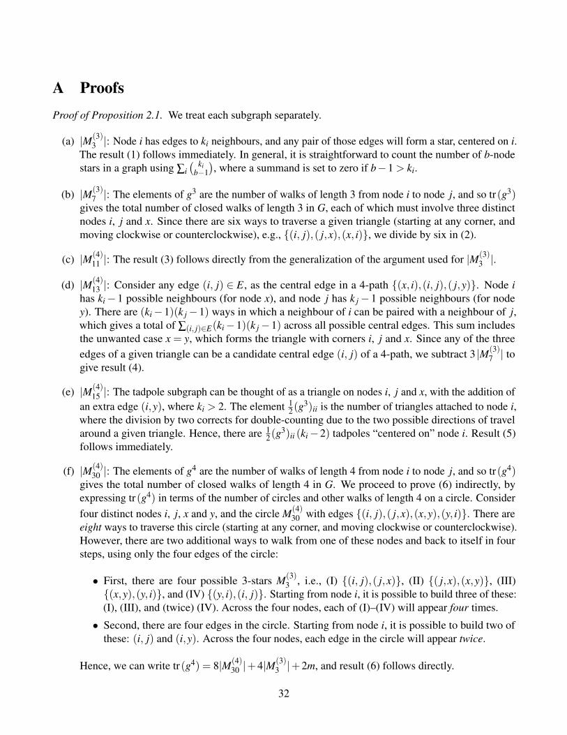
A ProofsProof of Proposition 2.1. We treat each subgraph separately.

(a) |M(3)3 |: Node i has edges to ki neighbours, and any pair of those edges will form a star, centered on i.

The result (1) follows immediately. In general, it is straightforward to count the number of b-nodestars in a graph using ∑i

( kib−1

), where a summand is set to zero if b−1 > ki.

(b) |M(3)7 |: The elements of g3 are the number of walks of length 3 from node i to node j, and so tr(g3)

gives the total number of closed walks of length 3 in G, each of which must involve three distinctnodes i, j and x. Since there are six ways to traverse a given triangle (starting at any corner, andmoving clockwise or counterclockwise), e.g., {(i, j),( j,x),(x, i)}, we divide by six in (2).

(c) |M(4)11 |: The result (3) follows directly from the generalization of the argument used for |M(3)

3 |.

(d) |M(4)13 |: Consider any edge (i, j) ∈ E, as the central edge in a 4-path {(x, i),(i, j),( j,y)}. Node i

has ki−1 possible neighbours (for node x), and node j has k j−1 possible neighbours (for nodey). There are (ki−1)(k j−1) ways in which a neighbour of i can be paired with a neighbour of j,which gives a total of ∑(i, j)∈E(ki−1)(k j−1) across all possible central edges. This sum includesthe unwanted case x = y, which forms the triangle with corners i, j and x. Since any of the threeedges of a given triangle can be a candidate central edge (i, j) of a 4-path, we subtract 3 |M(3)

7 | togive result (4).

(e) |M(4)15 |: The tadpole subgraph can be thought of as a triangle on nodes i, j and x, with the addition of

an extra edge (i,y), where ki > 2. The element 12(g

3)ii is the number of triangles attached to node i,where the division by two corrects for double-counting due to the two possible directions of travelaround a given triangle. Hence, there are 1

2(g3)ii (ki−2) tadpoles “centered on” node i. Result (5)

follows immediately.

(f) |M(4)30 |: The elements of g4 are the number of walks of length 4 from node i to node j, and so tr(g4)

gives the total number of closed walks of length 4 in G. We proceed to prove (6) indirectly, byexpressing tr(g4) in terms of the number of circles and other walks of length 4 on a circle. Considerfour distinct nodes i, j, x and y, and the circle M(4)

30 with edges {(i, j),( j,x),(x,y),(y, i)}. There areeight ways to traverse this circle (starting at any corner, and moving clockwise or counterclockwise).However, there are two additional ways to walk from one of these nodes and back to itself in foursteps, using only the four edges of the circle:

• First, there are four possible 3-stars M(3)3 , i.e., (I) {(i, j),( j,x)}, (II) {( j,x),(x,y)}, (III)

{(x,y),(y, i)}, and (IV) {(y, i),(i, j)}. Starting from node i, it is possible to build three of these:(I), (III), and (twice) (IV). Across the four nodes, each of (I)–(IV) will appear four times.

• Second, there are four edges in the circle. Starting from node i, it is possible to build two ofthese: (i, j) and (i,y). Across the four nodes, each edge in the circle will appear twice.

Hence, we can write tr(g4) = 8|M(4)30 |+4|M(3)

3 |+2m, and result (6) follows directly.

32

(a) 4-star M(4)11 . (b) Tadpole M(4)

15 . (c) Diamond M(4)31 . (d) 4-complete M(4)

63 .

Figure A.1: Illustrative nestings of the 4-star subgraph. There is one way in which one edge can be removed fromthe tadpole to create a 4-star, two ways in which two edges can be removed from the diamond, and fourways in which three edges can be removed from the 4-complete.

(g) |M(4)31 |: We can think of a diamond on nodes i, j, x, and y as two distinct triangles with a common

edge (i, j). Given this common edge, (g2)i j (g)i j represents the number of walks of length 2 betweeni and j, i.e., the number of distinct triangles in G that contain (i, j). A diamond is formed by anytwo of these triangles, and so

((g2)i j (g)i j2

)gives the number of distinct diamonds that can be built

from a common edge (i, j). Summing across all pairs of nodes i and j will give twice the number ofdiamonds in G, since the edge (i, j) has two endpoints. We divide the sum by two to give result (7).

Proof of 4-complete subgraph count formula (8). Consider a triangle subgraph M(3)7 comprised of nodes

j, x and y. Let each node be in the neighbourhoood ΓG(i) of some node i such that i 6= j 6= x 6= y. Hence,the four nodes i, j, x and y, and the edges between them, form a 4-complete subgraph M(4)

63 . The quantity16 tr(g3

−i) gives the number of 4-complete subgraphs that contain node i, where g−i is the adjacency matrixinduced by the neighbourhood of i. By symmetry, summing across all nodes i will give four times the totalcount of 4-complete subgraphs in the graph, and so we divide the sum by four to give result (8).

Proof of Proposition 2.3. In each case, the non-nested subgraph count of H ′ is found by considering allsubgraphs H on the same set of b nodes as H, such that H ′ ⊂ H, and noting the number of ways in whichedges can be removed from H to obtain H ′. The non-nested subgraph count |M(b)

a | equals |M(b)a | with a

correction that accounts for nesting in “larger” subgraphs. For example, the 4-star M(4)11 is nested in the

tadpole M(4)15 , the diamond M(4)

31 and the 4-complete M(4)63 , as illustrated in Figure A.1. We continue to use

(2) and (8) for the nested triangle and 4-complete. We treat each subgraph separately but, for convenienceof exposition, not in order.

[insert Figure A.1 here]

(a) |M(3)3 |: To create a 3-star, there are three ways to remove one edge from the triangle. Result (10)

follows immediately.

(b) |M(4)31 |: To create a diamond, there are six ways to remove one edge from the 4-complete. Result

(15) follows immediately.

33

(c) |M(4)30 |: To create a 4-circle, there is one way to remove one edge from the diamond, and three ways

to remove two edges (with no common nodes) from the 4-complete. Hence,

|M(4)30 |= |M

(4)30 |− |M

(4)31 |−3 |M(4)

63 |,

and (14) follows from (15).

(d) |M(4)15 |: To create a tadpole, there are four ways to remove one edge from the diamond, and twelve

ways to remove two edges (with a common node) from the 4-complete. Hence,

|M(4)15 |= |M

(4)15 |−4 |M(4)

31 |−12 |M(4)63 |,

and (13) follows from (15).

(e) |M(4)13 |: To create a 4-path, there are two ways to remove one edge from a tadpole, four ways to

remove one edge from a 4-circle, six ways to remove two edges from a diamond, and twelve waysto remove three edges from a 4-complete. So,

|M(4)13 |= |M

(4)13 |−2 |M(4)

15 |−4 |M(4)30 |−6 |M(4)

31 |−12 |M(4)63 |,

and (12) follows from (13), (14) and (15).

(f) |M(4)11 |: As illustrated in Figure A.1, to create a 4-star, there is one way to remove one edge from a

tadpole, two ways to remove two edges from a diamond, and four ways to remove three edges (atriangle) from the 4-complete. Then,

|M(4)11 |= |M

(4)11 |− |M

(4)15 |−2 |M(4)

31 |−4 |M(4)63 |,

and (11) follows from (13) and (15).

Proof of Proposition 2.4. For each of the statements in the Proposition, we could present a formal proof.For example, consider the expected number of triangles (see Proposition 2.4). For every subgraphS ⊂ G(n, p), let ZS be the event “S is a triangle”, and let XS be its indicator random variable. Then,E(XS) = Pr(ZS) = p3, where Pr(·) is the probability of an event. Define Y = ∑|V (S)|=3 XS. By linearity ofexpectation, E(Y ) = ∑|V (S)|=3 E(XS), and the result follows. Alternatively, we could directly specialize theformulae in Proposition 2.1 to Kn. For example, the number of triangles is generally given by 1

6 tr(g3), andit is easy to see that (g3)ii = (n−1)(n−2) for Kn, so that 1

6 tr(g3) =(n

3

). However, we instead present

more informal proofs of each statement, based directly on the properties of Kn, that we feel are moreintuitive and accessible. Using linearity of expectation as above, it is sufficient to find the number of eachsubgraph S of interest in Kn, and then to multiply this count by p|E(S)| to give the count in G(n, p).

(a) |M(3)3 |: Each node in Kn can be the center of the 3-star, giving n

(n−12

)= 3(n

3

)3-stars in Kn.

(b) |M(3)7 |: There are

(n3

)triangles in Kn.

34

(c) |M(4)11 |: Each of the n nodes in Kn can be the center of the 4-star, and so there are a total of

n(n−1

3

)= 4(n

4

)4-stars in Kn. This is a direct generalization of the proof of |M(3)

3 |.

(d) |M(4)13 |: We can choose 4 nodes in

(n4

)ways, and they can be linked by a maximum of 6 edges. There

are(6

3

)= 20 combinations of 3 edges on these 4 nodes, including 4 that will give a triangle (and an

isolated node) and 4 that will give a 4-star. Hence, there are 12 possible 4-paths on 4 nodes.

(e) |M(4)15 |: There are

(n3

)triangles in Kn. Any of the 3 corners of each triangle can be the “center”

(degree 3 node) of a tadpole, and links to (n−3) other nodes, forming a tadpole in each case.

(f) |M(4)30 |: The argument is similar to that used for |M(4)

13 |. We can choose 4 nodes in(n

4

)ways, and they

can be linked by a maximum of 6 edges. There are(6

4

)= 15 combinations of 4 edges on these 4

nodes, including 12 that will give a tadpole (there are 4 triangles, and 3 ways to add an additionaledge for each). Hence, there are 3 possible circles on 4 nodes. We can also show this directly bylabelling the nodes of a circle i, j, x and y: corner i can have opposite (non-adjacent) corner j, x or y.

(g) |M(4)31 |: We can choose 4 nodes in

(n4

)ways, and there are 6 ways to link them with 5 edges, each of

which will generate a diamond with a different common edge (between the two triangles).

(h) |M(4)63 |: We can choose 4 nodes in

(n4

)ways, and there is only one way to link them with 6 edges.

35

B Additional Figures

36


7 .

(c) 4-star M(4)11 . (d) 4-path M(4)

13 .


30 .

(g) Diamond M(4)31 . (h) 4-complete M(4)

63 .

Figure B.1: Nested subgraph counts by analytic formulae (Section 2.2).

37


7 .

(c) 4-star M(4)11 . (d) 4-path M(4)

13 .


30 .

(g) Diamond M(4)31 . (h) 4-complete M(4)

63 .

Figure B.2: Log–log plots of number of edges m against nested subgraph count |M(b)a | (Section 2.3).

38

(a) 5-star M(5)75 . (b) Cricket M(5)

79 .

(c) Bull M(5)87 . (d) Banner M(5)

94 .

(e) 5-circle M(5)236. (f) 6-star M(6)

1099.

Figure B.3: Log–log plots of number of edges m against nested subgraph count |M(b)a | (Section 2.3.2).

39

Figure B.4: Averaging of scaling factor by regression fit, for toy regime-switching model (Section 2.3.3), illustratedusing simulated data, with l = 4, . . . ,n = 30, and breakpoint n? = 20 between Regimes 1 and 2.

(a) 1999Q4. (b) 2003Q4.

(c) 2007Q4. (d) 2013Q4.

Figure B.5: Gaussian kernel density estimates corresponding to the degree distribution P(k) of Southwest’s network,not correcting for edge-effects; and the binomial degree distribution of the Erdos-Renyi graph G(n, p)with edge-formation probability p = d(G) (Section 2.4.2). Note that the Gaussian kernel does notcorrect for potential edge-effects at k = 0.

40

C Subgraph Notation

We denote b-node subgraphs by M(b)a , where a is a decimal number defined as follows (see Example C.1):

1. Choose an arbitrary labelling of the nodes of the subgraph (from 1 to b), to give a subgraph G′.

2. Find all subgraphs that are isomorphic to G′, and list their adjacency matrices.

3. Use the upper-triangular elements of each adjacency matrix, including leading zeros, to give binaryrepresentations, e.g., 1110002 and 1001102 and 0101012 and 0010112, respectively.

4. Find the decimal representation of each binary number, and set b equal to the minimum of these,e.g., in the example, we have 5610 and 3810 and 2110 and 1110; so, we use M(4)

11 to denote the 4-star.

Example C.1 (Notation).

=

1 2 3 4

1 0 1 1 12 1 0 0 03 1 0 0 04 1 0 0 0

∼=

1 2 3 4

1 0 1 0 02 1 0 1 13 0 1 0 04 0 1 0 0

∼=

1 2 3 4

1 0 0 1 02 0 0 1 03 1 1 0 14 0 0 1 0

∼=

1 2 3 4

1 0 0 0 12 0 0 0 13 0 0 0 14 1 1 1 0

.

41

References[1] V. Aguirregabiria and C.-Y. Ho. A dynamic oligopoly game of the US airline industry: Estimation

and policy experiments. Journal of Econometrics, 168:156–173, 2012.

[2] N. Alon, R. Yuster, and U. Zwick. Finding and counting given length cycles. Algorithmica, 17:209–223, 1997.

[3] U. Alon. Network motifs: Theory and experimental approaches. Nature Reviews Genetics, 8:450–461, 2007.

[4] O. Angel, R. van der Hofstad, and C. Holmgren. Limit laws for self-loops and multiple edgesin the configuration model. Technical Report arXiv:1603.07172v2, 2017. (available at: http:

//arxiv.org/abs/1603.07172 ).

[5] M. Angeles Serrano, D. Krioukov, and M. Boguna. Self-similarity of complex networks and hiddenmetric spaces. Physical Review Letters, 100:078701, 2008.

[6] A.-L. Barabasi. Network Science. Cambridge University Press, 2016.

[7] A. Barrat, M. Barthelemy, R. Pastor-Satorras, and A. Vespignani. The architecture of complexweighted networks. PNAS, 101:3747–3752, 2004.

[8] A. Bjorklund, R. Pagh, V. Vassilevska Williams, and U. Zwick. Listing triangles. In ICALP 14(International Colloquium on Automata, Languages, and Programming), 2014.

[9] F. Bloch, M.O. Jackson, and P. Tebaldi. Centrality measures in networks. Technical ReportarXiv:1608.05845v1, 2016. (available at: http://arxiv.org/pdf/1608.05845v1.pdf ).

[10] G. Bounova and O. de Weck. Overview of metrics and their correlation patterns for multiple-metrictopology analysis on heterogeneous graph ensembles. Physical Review E, 85:016117, 2012.

[11] G.A. Bounova. Topological evolution of networks: Case studies in the US airlines and languageWikipedias. PhD thesis, Massachusetts Institute of Technology, 2009.

[12] C. Bron and J. Kerbosch. Algorithm 457: Finding all cliques of an undirected graph. Communicationsof the ACM, 16:575–577, 1973.

[13] L. Chen, X. Qu, M. Cao, Y. Zhou, W. Li, B. Liang, W. Li, W. He, C. Feng, X. Jia, and Y. He.Identification of breast cancer patients based on human signaling network motifs. Scientific Reports,3:3368, 2013.

[14] S. Chu and J. Cheng. Triangle listing in massive networks. ACM Transactions on KnowledgeDiscovery from Data, 6:17:1–17:32, 2012.

[15] F. Ciliberto and E. Tamer. Market structure and multiple equilibria in airline markets. Econometrica,77:1791–1828, 2009.

42

http://arxiv.org/abs/1603.07172


http://arxiv.org/pdf/1608.05845v1.pdf

[16] A. Clauset, C.R. Shalizi, and M.E.J. Newman. Power-law distributions in empirical data. SIAMReview, 51:661–703, 2009.

[17] D. Coppersmith and S. Winograd. Matrix multiplication via arithmetic progressions. Journal ofSymbolic Computation, 9:251–280, 1990.

[18] T.H. Cormen, C.E. Leiserson, R.L. Rivest, and C. Stein. Introduction to Algorithms. MIT Press, 3rdedition, 2009.

[19] M. Dai, Q. Liu, and K. Serfes. Is the effect of competition on price dispersion non-monotonic?Evidence from the U.S. airline industry. Review of Economics and Statistics, 96:161–170, 2014.

[20] R. Diestel. Graph Theory. Springer, 5th edition, 2017.

[21] R. Dobrin, Q.K. Beg, A.-L. Barabasi, and Z.N. Oltvai. Aggregation of topological motifs in theEscherichia coli transcriptional regulatory network. BMC Bioinformatics, 5:10, 2004.

[22] A. Dossin and S. Lawford. Weighted network centrality measures: with application to U.S. domesticairlines. DEVI / ENAC unpublished report, 2017.

[23] S.N. Durlauf. Complexity and empirical economics. Economic Journal, 115:F225–F243, 2005.

[24] R.W. Eglese. Simulated annealing: A tool for operational research. European Journal of OperationalResearch, 46:271–281, 1990.

[25] E. Estrada. The Structure of Complex Networks. Oxford University Press, 2011.

[26] E. Estrada and P.A. Knight. A First Course in Network Theory. Oxford University Press, 2015.

[27] E. Estrada and J.A. Rodrıguez-Velazquez. Subgraph centrality in complex networks. PhysicalReview E, 71:056103, 2005.

[28] Facebook. Press Release: Facebook Reports Second Quarter 2017 Results. http://investor.

fb.com/investor-news/default.aspx July 26 2017. http://s21.q4cdn.com/399680738/

files/doc_news/2017/FB-Q2’17-Earnings-Release.pdf (Retrieved on September 6, 2017).

[29] D.C. Fisher and J. Ryan. Bounds on the number of complete subgraphs. Discrete Mathematics, 103:313–320, 1992.

[30] X. Gabaix. Power laws in economics and finance. Annual Review of Economics, 1:255–293, 2009.

[31] X. Gabaix. Power laws in economics: An introduction. Journal of Economic Perspectives, 30:185–206, 2016.

[32] X. Gabaix, P. Gopikrishnan, V. Plerou, and H.E. Stanley. A theory of power-law distributions infinancial market fluctuations. Nature, 423:267–270, 2003.

[33] A. Goolsbee and C. Syverson. How do incumbents respond to the threat of entry? Evidence from themajor airlines. Quarterly Journal of Economics, 123:1611–1633, 2008.

43

http://investor.fb.com/investor-news/default.aspx

http://investor.fb.com/investor-news/default.aspx

http://s21.q4cdn.com/399680738/files/doc_news/2017/FB-Q2'17-Earnings-Release.pdf

http://s21.q4cdn.com/399680738/files/doc_news/2017/FB-Q2'17-Earnings-Release.pdf

[34] F. Harary and A.J. Schwenk. The spectral approach to determining the number of walks in a graph.Pacific Journal of Mathematics, 80:443–449, 1979.

[35] F. Hayot and C. Jayaprakash. A feedforward loop motif in transcriptional regulation: Induction andrepression. Journal of Theoretical Biology, 234:133–143, 2005.

[36] P.J. Ingram, M.P.H. Stumpf, and J. Stark. Network motifs: Structure does not determine function.BMC Genomics, 7:108, 2006.

[37] S. Isihara, K. Fujimoto, and T. Shibata. Cross talking of network motifs in gene regulation thatgenerates temporal pulses and spatial stripes. Genes to Cells, 10:1025–1038, 2005.

[38] R. Itzhack, Y. Mogilevski, and Y. Louzoun. An optimal algorithm for counting network motifs.Physica A, 381:482–490, 2007.

[39] S. Itzkovitz and U. Alon. Subgraphs and network motifs in geometric networks. Physical Review E,71:026117, 2005.

[40] S. Itzkovitz, R. Levitt, N. Kashtan, R. Milo, M. Itzkovitz, and U. Alon. Coarse-graining andself-dissimilarity of complex networks. Physical Review E, 71:016127, 2005.

[41] M.O. Jackson. Social and Economic Networks. Princeton University Press, 2008.

[42] M.O. Jackson. An overview of social networks and economic applications. In J. Benhabib, A. Bisin,and M.O. Jackson, editors, Handbook of Social Economics. North Holland, 2011.

[43] D. Jungnickel. Graphs, Networks and Algorithms. Springer, 3rd edition, 2008.

[44] N. Kashtan, S. Itzkovitz, R. Milo, and U. Alon. Topological generalizations of network motifs.Physical Review E, 70:031909, 2004.

[45] N. Kashtan, S. Itzkovitz, R. Milo, and U. Alon. Efficient sampling algorithm for estimating subgraphconcentrations and detecting network motifs. Bioinformatics, 20:1746–1758, 2004.

[46] S. Khakabimamaghani, I. Sharafuddin, N. Dichter, I. Koch, and A. Masoudi-Nejad. QuateXelero:An accelerated exact network motif detection algorithm. PloS ONE, 8:e68073, 2013.

[47] J. Leskovec and A. Krevl. SNAP Datasets: Stanford Large Network Dataset Collection. http:

//snap.stanford.edu/data 2017.

[48] J. Lin and Y. Ban. The evolving network structure of US airline system during 1990-2010. PhysicaA, 410:302–312, 2014.

[49] O. Lordan, J.M. Sallan, and P. Simo. Study of the topology and robustness of airline route networksfrom the complex network approach: a survey and research agenda. Journal of Transport Geography,37:112–120, 2014.

[50] S. Mangan and U. Alon. Structure and function of the feed-forward loop network motif. PNAS, 100:11980–11985, 2003.

44

http://snap.stanford.edu/data

http://snap.stanford.edu/data

[51] R. Milo, S. Shen-Orr, S. Itzkovitz, N. Kashtan, D. Chklovskii, and U. Alon. Network motifs: Simplebuilding blocks of complex networks. Science, 298:824–827, 2002.

[52] A. Mrvar and V. Batagelj. Analysis and visualization of large networks with program package Pajek.Complex Adaptive Systems Modeling, 4:6, 2016.

[53] M.E.J. Newman. The structure and function of complex networks. SIAM Review, 45:167–256, 2003.

[54] M.E.J. Newman. Random graphs with clustering. Physical Review Letters, 103:058701, 2009.

[55] E. Orduna-Malea, J.M. Ayllon, A. Martın-Martın, and E.D. Lopez-Cozar. Methods for estimatingthe size of Google Scholar. Technical Report arXiv:1506.03009v1, 2015. (available at: http:

//arxiv.org/abs/1506.03009 ).

[56] R.J. Prill, P.A. Iglesias, and A. Levchenko. Dynamic properties of network motifs contribute tobiological network organization. PLoS Biology, 3:1881–1892, 2005.

[57] C. Roucolle, T. Seregina, and M. Urdanoz. Measuring airline networks: Comprehensive indicators.ENAC unpublished report, 2017.

[58] A. Rucinski. When are small subgraphs of a random graph normally distributed? Probability Theoryand Related Fields, 78:1–10, 1988.

[59] W.E. Schlauch and K.A. Zweig. Influence of the null-model on motif detection. In ASONAM 15(Advances in Social Networks Analysis and Mining), 2015.

[60] F. Schreiber and H. Schwobbermeyer. Frequency concepts and pattern detection for the analysis ofmotifs in networks. In Transactions on Computational Systems Biology III, pages 89–104, 2005.

[61] S.S. Shen-Orr, R. Milo, S. Mangan, and U. Alon. Network motifs in the transcriptional regulationnetwork of Escherichia coli. Nature Genetics, 31:64–68, 2002.

[62] C. Song, S. Havlin, and H.A. Makse. Self-similarity of complex networks. Nature, 433:392–395,2005.

[63] O. Sporns and R. Kotter. Motifs in brain networks. PLoS Biology, 2:1910–1918, 2004.

[64] N.T.L. Tran, S. Mohan, Z. Xu, and C.-H. Huang. Current innovations and future challenges ofnetwork motif detection. Briefings in Bioinformatics, 16:497–525, 2014.

[65] Twitter. Press Release: Twitter Announces Second Quarter 2017 Results. http://investor.

twitterinc.com/results.cfm July 27 2017. http://files.shareholder.com/downloads/

AMDA-2F526X/5135079665x0x951003/11DEB964-E7A5-43F8-96E2-D074A947255B/TWTR_

Q2_17_Earnings_Press_Release.pdf (Retrieved on September 6, 2017).

[66] V. Vassilevska. Efficient algorithms for clique problems. Information Processing Letters, 109:254–257, 2009.

[67] V. Vassilevska Williams. Multiplying matrices in O(n2.373) time. Mimeo, Available at: \http:

//people.csail.mit.edu/virgi/matrixmult-f.pdf 2014.

45



http://investor.twitterinc.com/results.cfm

http://investor.twitterinc.com/results.cfm

http://files.shareholder.com/downloads/AMDA-2F526X/5135079665x0x951003/11DEB964-E7A5-43F8-96E2-D074A947255B/TWTR_Q2_17_Earnings_Press_Release.pdf



\ http://people.csail.mit.edu/virgi/matrixmult-f.pdf

\ http://people.csail.mit.edu/virgi/matrixmult-f.pdf

[68] V. Vassilevska Williams, J.R. Wang, R. Williams, and H. Yu. Finding four-node subgraphs in triangletime. In SODA 15 (ACM-SIAM Symposium on Discrete Algorithms), 2015.

[69] T. Verma, N.A.M. Araujo, and H.J. Herrmann. Revealing the structure of the world airline network.Scientific Reports, 4:5638, 2014.

[70] T. Verma, F. Russmann, N.A.M. Araujo, J. Nagler, and H.J. Herrmann. Emergence of core-peripheriesin networks. Nature Communications, 7:10441, 2016.

[71] D.J. Watts. Networks, dynamics, and the small-world phenomenon. American Journal of Sociology,105:493–527, 1999.

[72] D.J. Watts and S.H. Strogatz. Collective dynamics of ‘small-world’ networks. Nature, 393:440–442,1998.

[73] E. Wong, B. Baur, S. Quader, and C.-H. Huang. Biological network motif detection: Principles andpractice. Briefings in Bioinformatics, 13:202–215, 2011.

[74] S.F. Wu, W.Y. Qian, J.W. Zhang, Y.B. Yang, Y. Liu, Y. Dong, Z.B. Zhang, Y.P. Zhu, and Y.J. Feng.Network motifs in the transcriptional regulation network of cervical carcinoma cells respond to EGF.Archives of Gynecology and Obstetrics, 287:771–777, 2013.

[75] S. Wuchty and P.F. Stadler. Centers of complex networks. Journal of Theoretical Biology, 223:45–53, 2003.

[76] D.R. Wuellner, S. Roy, and R.M. D’Souza. Resilience and rewiring of the passenger airline networksin the United States. Physical Review E, 82:056101, 2010.

[77] E. Yeger-Lotem, S. Sattath, N. Kashtan, S. Itzkovitz, R. Milo, R.Y. Pinter, and U. Alon. Networkmotifs in integrated cellular networks of transcription–regulation and protein–protein interaction.PNAS, 101:5934–5939, 2004.

46

Documents

Subgraphs and Motifs in a Dynamic Airline Network