Subcubic Equivalences BetweenGraph Centrality Problems, APSP and Diameter

Amir Abboud∗ Fabrizio Grandoni† Virginia Vassilevska Williams‡

AbstractMeasuring the importance of a node in a network is a majorgoal in the analysis of social networks, biological systems,transportation networks etc. Different centrality measures havebeen proposed to capture the notion of node importance. Forexample, the center of a graph is a node that minimizes themaximum distance to any other node (the latter distance isthe radius of the graph). The median of a graph is a nodethat minimizes the sum of the distances to all other nodes.Informally, the betweenness centrality of a node w measures thefraction of shortest paths that have w as an intermediate node.Finally, the reach centrality of a node w is the smallest distancer such that any s-t shortest path passing through w has either sor t in the ball of radius r around w.

The fastest known algorithms to compute the center andthe median of a graph, and to compute the betweenness or reachcentrality even of a single node take roughly cubic time in thenumber n of nodes in the input graph. It is open whether theseproblems admit truly subcubic algorithms, i.e. algorithms withrunning time O(n3−δ) for some constant δ > 01.

We relate the complexity of the mentioned centrality prob-lems to two classical problems for which no truly subcubic al-gorithm is known, namely All Pairs Shortest Paths (APSP) andDiameter. We show that Radius, Median and Betweenness Cen-trality are equivalent under subcubic reductions to APSP, i.e.that a truly subcubic algorithm for any of these problems im-plies a truly subcubic algorithm for all of them. We then showthat Reach Centrality is equivalent to Diameter under subcubicreductions. The same holds for the problem of approximatingBetweenness Centrality within any constant factor. Thus the lat-ter two centrality problems could potentially be solved in trulysubcubic time, even if APSP requires essentially cubic time.

1 IntroductionIdentifying the importance of nodes in networks is a majorgoal in the analysis of social networks (e.g., citation net-works, recommendation networks, or friendship circles),biological systems (e.g., protein interaction networks),computer networks (e.g., the Internet or peer-to-peer net-works), transportation networks (e.g., public transporta-tion or road networks), etc. A variety of graph theoreticnotions of node importance have been proposed, amongthe most relevant ones: betweenness centrality [20], graphcentrality [29], closeness centrality [47], and reach cen-trality [28].

∗Stanford University, abboud@cs.stanford.edu.†IDSIA, University of Lugano, fabrizio@idsia.ch. Partially

supported by the ERC Starting Grant NEWNET 279352.‡Stanford University, virgi@cs.stanford.edu. Supported by

NSF Grant CCF-1417238, BSF Grant BSF:2012338 and a Stanford SOEHoover Fellowship.

1The O notation suppresses poly-logarithmic factors in n and M .

The graph centrality of a node w is the inverse ofits maximum distance to any other node. The closenesscentrality of w is the inverse of the total distance of wto all the other nodes. The reach centrality of w is themaximum distance between w and the closest endpointof any s-t shortest path passing through w. Informally,the betweenness centrality of w measures the fraction ofshortest paths having w as an intermediate node.

In this paper we study four fundamental graph cen-trality computational problems associated with the men-tioned centrality measures. Let G = (V,E) be an n-nodem-edge (directed or undirected) graph, with integer edgeweights w : E → 0, . . . ,M for some M ≥ 12. LetdG(s, t) denote the distance from node s to node t, andlet us use d(s, t) instead when G is clear from the context.Let also σs,t be the number of distinct shortest paths froms to t, and σs,t(b) be the number of such paths that usenode b as an intermediate node.

• The Radius problem is to compute R∗ :=minr∗∈V maxv∈V d(r∗, v) (radius of the graph).

• The Median problem is to compute M∗ :=minm∗∈V

∑v∈V d(m∗, v).

• The Reach Centrality problem (for a given node b) isto compute

RC(b) = maxs,t∈V :

d(s,t)=d(s,b)+d(b,t)

mind(s, b), d(b, t).

• The Betweenness Centrality problem (for a givennode b) is to compute

BC(b) :=∑

s,t∈V−b, s=t

σs,t(b)

σs,t.

All of these notions are related in one way or anotherto shortest paths. In particular, we can solve the first threeproblems by running an algorithm for the classical All-Pairs Shortest Paths problem (APSP) on the underlyinggraph and doing a negligible amount of post-processing.The same holds for Betweenness Centrality by assuming

2Though we focus here on non-negative weights, our results can beextended to the case of directed graphs with possibly negative weightsand no negative cycles.

that shortest paths are unique: we will next make this as-sumption unless differently stated3. Using the best knownalgorithms for APSP [55], this leads to a slightly subcu-bic (by an no(1) factor) running time for the consideredproblems, and no faster algorithm is known.

Each of these problems however only asks for thecomputation of a single number. It is natural to ask, issolving APSP necessary? Could it be that these problemsadmit much more efficient solutions? In particular, dothey admit a truly subcubic4 algorithm?

Besides the fundamental interest in understanding therelations between such basic computational problems (canRadius be solved truly faster than APSP?), these ques-tions are well motivated from a practical viewpoint. Asevidence to the necessity of faster algorithms for the men-tioned centrality problems, we remark that some paperspresenting algorithms for Betweenness Centrality [6] andMedian [30] have received more than a thousand citationseach.

1.1 Approach. In this paper we address these ques-tions with an approach which can be viewed as a refine-ment of NP-completeness. The approach strives to prove,via combinatorial reductions, that improving on a givenupper bound for a computational problem B would yieldbreakthrough algorithms for many other famous and well-studied problems. At high-level, the idea is to consider agiven prototypical problem A for which the fastest knownalgorithm has running time O(nc) (here n is a size pa-rameter). Then we show that a O(nc−ε)-time algorithmfor a second problem B, for some constant ε > 0, wouldimply a O(nc−δ)-time algorithm for problem A for someother constant δ > 0. This can be used as evidence that aO(nc−ε) time algorithm for problem B is unlikely to ex-ist (or at least very hard to find). For c = 3 a reductionof the above kind is called a subcubic reduction [53] fromA to B. We say that two problems A and B are equiva-lent under subcubic reductions if there exists a subcubicreduction from A to B and from B to A. In other terms, atruly subcubic algorithm for one problem implies a trulysubcubic algorithm for the other and vice versa.

Vassilevska Williams and Williams [53] introducedthis approach to the realm of Graph Algorithms to showthe subcubic equivalence between APSP and a list ofseven other problems, including: deciding if an edge-weighted graph has a triangle with negative total weight(Negative Triangle), deciding if a given matrix defines ametric, and the Replacement Paths problem [27, 46, 51,54]. Other examples of this approach [1, 2, 44] include

3In the case of multiple shortest paths, the fastest known algorithmfor Betweenness Centrality takes O(n4) time; please see the discussionin the related work section.

4We recall that a truly subcubic algorithm is an algorithm withrunning time O(n3−δ) for some constant δ > 0.

the famous results on 3-SUM hardness starting with thework of Gajentaan and Overmars [21].

In this paper we exploit both APSP and Diameter asour prototypical problem and prove a collection of sub-cubic equivalences with the above graph centrality prob-lems. Recall that the Diameter problem is to compute thelargest distance in the graph. There is a trivial subcubicreduction from Diameter to APSP and, although no trulysubcubic algorithm is known for Diameter, finding a re-duction in the opposite direction is one of the big openquestions in this area: can we compute the largest distancefaster than we can compute all the distances?

1.2 Subcubic equivalences with APSP. Our first mainresult is to show that Radius, Median and BetweennessCentrality are equivalent to APSP under subcubic reduc-tions! Therefore, we add three quite different problems tothe list of APSP-hard problems [53] and if any of theseproblems can be solved in truly subcubic time then all ofthem can.

THEOREM 1.1. Radius, Median, and Betweenness Cen-trality are equivalent to APSP under subcubic reductions.

Unfortunately, this is strong evidence that a truly sub-cubic algorithm for computing these centrality measuresis unlikely to exist (or at least very hard to find) since itwould imply a huge and unexpected algorithmic break-through.

We find the APSP-hardness result for Radius quite in-teresting since, prior to our work, there was no good rea-son to believe that Radius might be a truly harder problemthan Diameter. Indeed, in terms of approximation algo-rithms, any known algorithm to approximate the diametercan be converted to also approximate the radius in undi-rected graphs within the same factor [3, 5, 10, 45]. Fur-thermore, the exact algorithms for Diameter and Radiusin graphs with small integer weights are also extremelysimilar [13]. Our results seem to indicate the followingbizarre phenomenon. In dense graphs, Radius seems tobe harder than Diameter, as it is actually equivalent toAPSP, whereas a Diameter/APSP equivalence seems elu-sive. In sparse graphs, however, Diameter seems moredifficult than Radius since a known reduction [45] fromCNF-SAT seems to imply that even approximating the Di-ameter in subquadratic time is hard. No such reduction isknown for Radius, and so far there is no evidence againsta subquadratic Radius algorithm in sparse graphs.

1.3 Subcubic equivalence with Diameter. Our sec-ond main result is to show that Reach Centrality and Di-ameter are equivalent under subcubic reductions.

THEOREM 1.2. Diameter and Reach Centrality areequivalent under subcubic reductions.

On the positive side, it is within the realm of possi-bility that Diameter is a truly easier problem than APSP,which would imply the same for Reach Centrality. On thenegative side, Theorem 1.2 shows that finding a subcu-bic algorithm for Reach Centrality is as hard as finding asubcubic algorithm for Diameter - a big open problem.

As a consequence of the tightness of our reductions,namely not only the number of nodes but also the largestabsolute weight is roughly preserved, we also obtain afaster algorithm for Reach Centrality in directed graphswith small integer weights.

THEOREM 1.3. There exists an O(Mnω) time algorithmfor Reach Centrality in directed graphs.

Above ω ∈ [2, 2.373) [12, 14, 22, 52] denotes fast matrixmultiplication exponent. The previous best algorithm forsmall integer weights, which is based on the solutionof APSP, takes time O(M0.681n2.575) [57]. This isinteresting in our opinion since Reach Centrality hasbeen used in some very fast (in practice) shortest pathsalgorithms [24, 25, 28].

1.4 Approximation algorithms. An approximatevalue of the mentioned graph centrality measures mightbe sufficiently good in practice. This is indeed the topicof several empirical works on Betweenness Centrality[4, 7, 23]. Furthermore, the mentioned practically fastshortest paths algorithms [24, 25, 28] can be adapted towork with approximate values of the reach centrality aswell. In this paper we formally study the approximabilityof the mentioned problems.

In more detail, given a graph centrality measure X ,our goal is to compute (quickly) a quantity x such that1αX ≤ x ≤ αX for some α ≥ 1 as small as possible (α isthe approximation factor). It is known how to solve APSPwithin a multiplicative error (1 + ε) in time O(nω) [56].This provides truly subcubic (1 + ε) approximation al-gorithms for Radius and Median. However, this approachdoes not help with Reach/Betweenness Centrality, since inthose measures almost shortest paths are irrelevant. Herewe present some negative and (conditionally) positive re-sults on the approximability of the latter two problems.

It is not hard to see that any approximation algorithmfor Reach/Betweenness Centrality can be used to deter-mine whether BC(b) > 0. We show that, while solvingthe latter problem for a single node is equivalent to Diam-eter, solving it for every node is at least as hard as APSP!As a consequence any approximation algorithm (for anyfinite α) to compute the reach/betweenness centrality ofall nodes implies a truly subcubic algorithm for APSP.

On the positive side, we show that (single-node) Ap-proximate Betweenness Centrality is equivalent to Di-ameter under subcubic reductions. This equivalence isquite strong: any truly subcubic approximation algorithm

with finite approximation factor for Betweenness Central-ity implies a truly subcubic Diameter algorithm, while atruly subcubic Diameter algorithm implies a truly sub-cubic (1 + ε)-approximation algorithm for BetweennessCentrality, for any constant ε > 0. Our reductions areMonte-Carlo, i.e. the resulting algorithm might fail toprovide the desired approximation with some small prob-ability. In more detail, we provide a subcubic reduction toDiameter to compute the exact value of the betweennesscentrality when that value is sufficiently small. For thecomplementary case, we use a non-trivial random sam-pling algorithm. Analogously to the case of Reach Cen-trality, this gives some more hope that a truly subcubic al-gorithm for Approximate Betweenness Centrality exists,however such algorithm is probably not easy to find. Partof the mentioned reductions are summarized in Figure 1.

1.5 Related Work. APSP is among the best stud-ied problems in Computer Science. If the edge weightsare non-negative, one can run Dijkstra’s algorithm [16]from every source node, and solve the problem in timeO(mn+n2 logn) (by implementing Dijkstra’s algorithmwith Fibonacci heaps [19]). Johnson [36] showed howto obtain the same running time in the case of negativeweights also (but no negative cycles). Pettie [41] im-proved the running time to O(mn+ n2 log logn) and to-gether with Ramachandran to O(mn logα(m,n)) [42].If the graph is undirected and the edge weights are in-tegers fitting in a word, one can solve the problem intime O(mn) in the word-RAM model [50]. In densegraphs the running time of these algorithms is O(n3).Slightly subcubic algorithms were developed as well,starting with the work of Fredman [18]. Following a longsequence of improvements (among others, [8, 31]), veryrecently Williams [55] obtained an algorithm with run-ning time O(n3/2Ω(

√logn)). Faster algorithms are known

for small integer weights bounded in absolute value byM : in undirected graphs APSP can be solved in O(Mnω)

time [49] and in directed graphs in O(n2(Mn)1

4−ω )time [57]. The result for the directed case can be refinedto O(M0.681n2.575) using fast rectangular matrix multi-plication [32].

As we already mentioned, for general edge-weightsthe fastest known algorithms for Diameter and Radiussolve APSP (hence taking roughly cubic time). In the caseof directed graphs with small integer weights boundedby M there are faster, O(Mnω) time algorithms (see[13] and the references therein). Faster approximationalgorithms are known. Aingworth et al. [3] showedhow to compute a (roughly) 3/2 approximation of thediameter in time O(m

√n+n2). The same approximation

factor and running time can be achieved for Radius inundirected graphs [5]. The running time for both Radiusand Diameter was reduced to O(m

√n) by Roditty and

3

Figure 1 The main subcubic reductions considered in this paper. Dashed arrows correspond to trivial reductions. Allthe remaining reductions are given in this paper, excluding the one from APSP to Negative Triangle which is takenfrom [53].

ReachCentrality

Approx. Betw.Centrality

DiameterAPSPNegativeTriangle

BetweennessCentrality

Radius

Median

Vassilevska Williams [45] (see also [10] for a refinementof the approximation factor). The authors also showthat a 3/2 − ε approximation for Diameter running intime O(m2−ε) (for any constant ε > 0) would implythat the Strong Exponential Time Hypothesis (SETH)of [33] fails, thus showing that improving on the 3/2-approximation factor while still using a fast algorithmwould be difficult.

The notion of betweenness centrality was introducedby Freeman in the context of social networks [20], andsince then became one of the most important graph cen-trality measures in the applications. For example, this no-tion is used in the analysis of protein networks [15, 35],social networks [40, 43], sexual networks [38], and terror-ist networks [11, 37]. From an algorithmic point of view,betweenness centrality was used to identify a highway-node hierarchy for routing in road networks [48]. Bran-des’ algorithm [6] computes the betweenness centrality ofall nodes in time O(mn + n2 logn). This result is basedon a counting variant of Dijkstra’s algorithm. We remarkthat [6], similarly to other papers in the area, neglectsthe bit complexity of the counters which store the num-ber of pairwise shortest paths. This is reasonable in prac-tice since the maximum number N of alternative short-est paths between two nodes tends to be small in manyof the applications. By considering also N , the runningtime grows by a factor O(logN) = O(n log n). Indeed,in some applications one can even assume that shortestpaths are unique (as we do in most of this paper). Theuniqueness of shortest paths is either a consequence oftie breaking rules (Canonical-Path Betweenness Central-ity problem [23]), or can be enforced by perturbing edgeweights [24]. However, the running time to compute theexact betweenness centrality can be prohibitive in practicefor very large networks even assuming the uniqueness ofshortest paths. For this reason, some work was devotedto the fast approximation of the betweenness centrality ofall nodes [4, 7, 23]. Those works are based on randompivot-sampling techniques. They do not provide any the-oretical bound on the approximation factor: this is not sur-

prising a posteriori, in view of our APSP-hardness results.In contrast, our results suggest a candidate way to obtaina provably fast and accurate algorithm for ApproximateBetweenness Centrality (for a single node). Our approachdeviates substantially from [4, 7, 23] for small values ofthe betweenness centrality.

The Reach Centrality notion was introduced by Gut-man [28] in the framework of practically fast algorithmsto solve the Single-Source Shortest Paths problem. In par-ticular, the values RC(b) can be used to filter out somenodes during an execution of Dijkstra’s algorithm. Thenotion of Reach Centrality is also used in other works onthe same topic [24, 25].

Eppstein and Wang [17] consider the problem ofapproximating the closeness centrality of all nodes. Theypresent a random-sampling-based O((m + n logn) log n

ε2 )time algorithm which w.h.p. computes estimates withinan additive error εD∗, where D∗ is the diameter of thegraph. The same problem is investigated in [7] from anexperimental point of view. The Median problem was alsostudied in a distance-oracle query model [9, 26, 34].

1.6 Preliminaries and Notation. W.l.o.g. we assumethat the considered graph G = (V,E) is connected, hencem ≥ n− 1. We make the usual assumption that the nodesof the considered graph are labelled with integers between0 and n−1, and where needed we implicitly assume that nis lower bounded by a sufficiently large constant. For twonodes u, v ∈ V , by uv we indicate either an undirectededge between u and v or an edge directed from u to v.The interpretation will be clear from the context.

We remark that, in our subcubic reductions, it wouldbe sufficient to preserve (modulo poly-logarithmic fac-tors) the number n of nodes only. However, wheneverpossible, we will also try to preserve (in the same sense)also m and M . In many cases we obtain extremely tightreductions that even allow us to obtain new faster algo-rithms, as is the case with Reach Centrality via our tightreduction to Diameter.

For a given node w ∈ V , we let Rad(w) :=

maxv∈V d(w, v) (eccentricity of w) and Med(w) :=∑v∈V d(w, v). A node w minimizing Rad(w) and

Med(w) is a center and a median of the graph, respec-tively.

In some claims we assume that a T (n,m) time,T (n,M) time, or T (n,m,M) time algorithm for someproblem is given. In all those claims we implicitlyassume that those running times are polynomial functionslower bounded by m. More generally, however, it issufficient for our proofs that O(m + T (O(n), O(m))) =O(T (n,m)) and similarly for the other cases.

Throughout this paper, with high probability (w.h.p.)means with probability at least 1− 1/nO(1).

2 Subcubic Equivalence with APSPIn this section we prove the subcubic equivalence betweenAPSP and the following problems: Radius, Median andBetweenness Centrality. As mentioned in the introduc-tion, reducing these problems to APSP is fairly straight-forward and here we will focus on the opposite reductions.

We exploit Negative Triangle as an intermediate sub-problem: determine whether a given undirected graphG = (V,E), with integer edge weights w : E →−M, . . . ,M, contains a triangle whose edges sum toa negative number; such a triangle is called a negativetriangle. The latter problem was shown to be equivalentto APSP under subcubic reductions in [53].

LEMMA 2.1. [53] Negative Triangle and APSP (in di-rected or undirected graphs) are equivalent under subcu-bic reductions.

In order to simplify our proofs, we assume that theinput instance of Negative Triangle satisfies the followingproperties:

1. Path lengths are even. This can be achieved bymultiplying the weights by a factor 2.

2. Any two nodes are connected by a path containingat most 2 edges. This can be achieved by adding adummy node r, and n edges of weight 2M betweenr and any other node. Observe that no new negativetriangle is created this way.

3. By appending at most n + 1 leaf nodes to r withedges of cost 2M , we can assume w.l.o.g. that thefinal number of nodes is 2k+1 for some integer k.

These reductions can be performed in linear time, theyincrease the number of nodes by O(n), the number ofedges by O(n), and the maximum absolute weight bya factor 2. Therefore, any algorithm with (polynomialand at least linear in m) running time O(T (n,m,M)) forthe modified instance, can be used to solve the originalinstance in time O(m + T (O(n),m + O(n), 2M)) =O(T (n,m,M)).

Combining the reductions below with Lemma 2.1proves Theorem 1.1.

2.1 Betweenness Centrality. We start with the reduc-tion to Betweenness Centrality.

LEMMA 2.2. Given a O(T (n,m)) time algorithm forBetweenness Centrality in directed or undirected graphs,there exists a O(T (n,m)) time algorithm for NegativeTriangle.

Proof. Let (G = (V,E), w) be the input instance of Neg-ative Triangle (reduced as described above). In particular,n = 2k+1 is the number of nodes of G.

We start with the simpler directed case (see also Fig-ure 2). We construct a weighted directed graph (G′, w′)as follows. Graph G′ contains four sets of nodes I , J , K ,and L (layers). Each layer contains a copy of each nodev ∈ V . Let vI be the copy of v in I , and define analo-gously vJ , vK and vL. Let Q = Θ(M) be a sufficientlylarge integer. For each edge uv ∈ E, we add to G′ theedges uIvJ , uJvK , and uKvL, and assign to those edgesweight 2Q+w(uv). We add to G′ a dummy node b, andedges vIb and bvL for any v ∈ V , of weight 3Q − 1 and3Q, respectively. We also add to G′ two sets of nodesZ = z0, . . . , zk and O = o0, . . . , ok. For any v ∈ V ,we add the following edges of weight 3Q − 1 to G′. Letv0, v1, . . . , vk be a binary representation of v (interpretedas an integer between 0 and n− 1 = 2k+1 − 1). For eachj = 0, . . . , k, we add edges vIzj and ojvL if vj = 0, andedges vIoj and zjvL otherwise. We also add edges ojzjand zjoj of weight 3Q− 1 for j = 0, . . . , k. Observe thatk = O(log n), hence there are O(n log n) edges of thelatter type.

On (G′, w′) we compute BC(b), and output YES tothe input Negative Triangle instance iff BC(b) < n. Therunning time of the algorithm is O(m+ T (O(n), O(m+n logn))) = O(T (n,m)). Let us prove its correctness.The only paths passing through b are of the form sI , b, tLand have weight 6Q−1. For s = t, there must exist a nodew ∈ Z ∪ O such that sI , w, tL is a path of cost 6Q − 2.Therefore, the only pairs of nodes that can contribute toBC(b) are of the form (sI , sL). The shortest path of typesI , vJ , wK , sL has weight at most 6Q−2 if s belongs to anegative triangle, and at least 6Q otherwise. ThereforeBCsI ,sL(b) = 1 if s does not belong to any negativetriangle, and BCsI ,sL(b) = 0 otherwise. The correctnessfollows.

In the undirected case, we use the same weightedgraph (G′, w′) as before, but removing edge directions(and leaving one copy of parallel edges). The rest ofthe algorithm is as before, and the running time triviallyremains O(T (n,m)). Proving correctness requires aslightly more complicated case analysis. Consider anypair s, t ∈ V − b. Suppose (s, t) /∈ (I × L) ∪ (L× I).

5

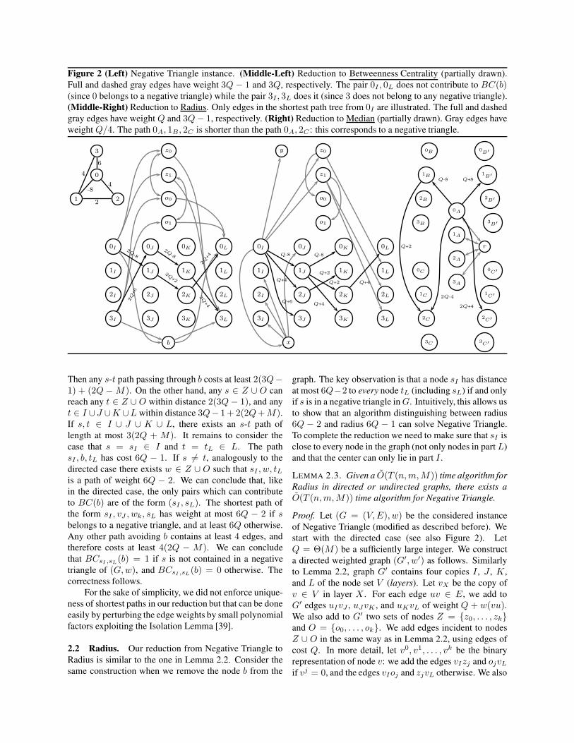
Figure 2 (Left) Negative Triangle instance. (Middle-Left) Reduction to Betweenness Centrality (partially drawn).Full and dashed gray edges have weight 3Q − 1 and 3Q, respectively. The pair 0I , 0L does not contribute to BC(b)(since 0 belongs to a negative triangle) while the pair 3I , 3L does it (since 3 does not belong to any negative triangle).(Middle-Right) Reduction to Radius. Only edges in the shortest path tree from 0I are illustrated. The full and dashedgray edges have weight Q and 3Q− 1, respectively. (Right) Reduction to Median (partially drawn). Gray edges haveweight Q/4. The path 0A, 1B, 2C is shorter than the path 0A, 2C : this corresponds to a negative triangle.

1 2

0

3

-84

6

4

2

3I

2I

1I

0I 0J

1J

2J

3J

0K

1K

2K

3K 3L

2L

1L

0L

z0

z1

o0

o1

b

2Q-8

2Q+2

2Q+4

2Q

+6

2Q-8

2Q+4

3I

2I

1I

0I 0J

1J

2J

3J

0K

1K

2K

3K 3L

2L

1L

0L

z0

z1

o0

o1

x

y

Q-8

Q+2

Q+4Q+4

Q+6

Q+2

Q-8

Q+4

0A

1A

2A

3A

0B

1B

2B

3B

0C

1C

2C

3C

0B′

1B′

2B′

3B′

0C′

1C′

2C′

3C′

r

Q-8 Q+8

Q+2

2Q-4

2Q+4

Then any s-t path passing through b costs at least 2(3Q−1) + (2Q − M). On the other hand, any s ∈ Z ∪ O canreach any t ∈ Z ∪ O within distance 2(3Q− 1), and anyt ∈ I ∪J ∪K ∪L within distance 3Q− 1+ 2(2Q+M).If s, t ∈ I ∪ J ∪ K ∪ L, there exists an s-t path oflength at most 3(2Q + M). It remains to consider thecase that s = sI ∈ I and t = tL ∈ L. The pathsI , b, tL has cost 6Q − 1. If s = t, analogously to thedirected case there exists w ∈ Z ∪ O such that sI , w, tLis a path of weight 6Q − 2. We can conclude that, likein the directed case, the only pairs which can contributeto BC(b) are of the form (sI , sL). The shortest path ofthe form sI , vJ , wk, sL has weight at most 6Q − 2 if sbelongs to a negative triangle, and at least 6Q otherwise.Any other path avoiding b contains at least 4 edges, andtherefore costs at least 4(2Q − M). We can concludethat BCsI ,sL(b) = 1 if s is not contained in a negativetriangle of (G,w), and BCsI ,sL(b) = 0 otherwise. Thecorrectness follows.

For the sake of simplicity, we did not enforce unique-ness of shortest paths in our reduction but that can be doneeasily by perturbing the edge weights by small polynomialfactors exploiting the Isolation Lemma [39].

2.2 Radius. Our reduction from Negative Triangle toRadius is similar to the one in Lemma 2.2. Consider thesame construction when we remove the node b from the

graph. The key observation is that a node sI has distanceat most 6Q−2 to every node tL (including sL) if and onlyif s is in a negative triangle in G. Intuitively, this allows usto show that an algorithm distinguishing between radius6Q − 2 and radius 6Q − 1 can solve Negative Triangle.To complete the reduction we need to make sure that sI isclose to every node in the graph (not only nodes in part L)and that the center can only lie in part I .

LEMMA 2.3. Given a O(T (n,m,M)) time algorithm forRadius in directed or undirected graphs, there exists aO(T (n,m,M)) time algorithm for Negative Triangle.

Proof. Let (G = (V,E), w) be the considered instanceof Negative Triangle (modified as described before). Westart with the directed case (see also Figure 2). LetQ = Θ(M) be a sufficiently large integer. We constructa directed weighted graph (G′, w′) as follows. Similarlyto Lemma 2.2, graph G′ contains four copies I , J , K ,and L of the node set V (layers). Let vX be the copy ofv ∈ V in layer X . For each edge uv ∈ E, we add toG′ edges uIvJ , uJvK , and uKvL of weight Q + w(vu).We also add to G′ two sets of nodes Z = z0, . . . , zkand O = o0, . . . , ok. We add edges incident to nodesZ ∪ O in the same way as in Lemma 2.2, using edges ofcost Q. In more detail, let v0, v1, . . . , vk be the binaryrepresentation of node v: we add the edges vIzj and ojvLif vj = 0, and the edges vIoj and zjvL otherwise. We also

add edges zjoj and ojzj of weight Q for all j = 0, . . . , k.Finally, we add nodes x and y, and for any v ∈ V we addedges vIx, xvI , and xvJ of weight Q, and edges vIy ofweight 3Q− 1.

We compute the radius R∗ of (G′, w′), and outputYES to the input instance of Negative Triangle iff R∗ ≤3Q − 1. The running time of the algorithm is O(m +T (O(n), O(m + n logn), O(M))) = O(T (n,m,M)).Let us prove its correctness. We first observe that thecenter r∗ of the graph belongs to I ∪ x since the othernodes cannot reach any node in I . Observe that d(x, y) =4Q − 1. On the other hand, any node sI is at distance atmost 2Q to nodes in Z ∪ O ∪ J ∪ x ∪ (L − sL), atmost 2Q + 2M to nodes in K (using the copy rJ of theroot node r), and exactly 3Q − 1 to node y. Note alsothat, if s belongs to a negative triangle, there exists an sI -sL path of the form sI , vJ , wK , sL with length at most3Q− 2. Otherwise one shortest sI -sL path passes troughnodes in Z ∪ O and has length 3Q. We can concludethat the center of the graph belongs to I , and that thecorresponding radius is upper bounded by 3Q−1 iff thereexists a negative triangle in (G,w).

In the undirected case we use precisely the same con-struction, but removing edge directions (and leaving onlyone copy of parallel edges). The algorithm is analogous aswell as its running time analysis. Its correctness can alsobe proved analogously. In more detail, similarly to the di-rected case, nodes in I can reach any other node withindistance at most 3Q+ 3M . Since d(y, x) = 4Q− 1, andd(s, y) ≥ (3Q−1)+(Q−M) for s /∈ I∪y, we can con-clude that r∗ ∈ I . Also in this case, for any node sI , itsmaximum distance to any other node is d(sI , y) = 3Q−1if s belongs to a negative triangle, and d(sI , sL) ≥ 3Qotherwise.

2.3 Median. The reduction to Median is based on arather different approach.

LEMMA 2.4. Given a O(T (n,M)) time algorithm forMedian in undirected or directed graphs, there exists aO(T (n,M)) time algorithm for Negative Triangle.

Proof. Let (G = (V,E), w) be the given instance ofNegative Triangle. First, consider the directed case (seealso Figure 2). We create a weighted directed graph(G′, w′). Graph G′ contains five copies A,B,B′, C, C′

of V . With the usual notation, vA is the copy of v in Aand similarly for the other sets. Let Q = Θ(M) be alarge enough integer. For any pair of nodes u, v, we addthe edges uAvB of weight Q + w(uv), uAvB′ of weightQ−w(uv), uAvC of weight 2Q−w(uv), uAvC′ of weight2Q + w(uv), and uBvC of weight Q + w(uv). In thisconstruction, when uv /∈ E (including the special caseu = v), we simply assume w(uv) = 2M . Furthermore,we add a dummy node r, and edges rvA and vAr of

weight Q/4 for any v ∈ V .In this graph we compute the median value M∗, and

output YES to the input instance of Negative Triangle iffM∗ < Q/4+(n−1)Q/2+6nQ. The running time of thealgorithm is O(m + T (O(n), O(M))) = O(T (n,M)).Let us show its correctness. Next d(·) denotes distancesin G′. Observe that the median node has to be in A ∪ rsince the remaining nodes cannot reach r. Note that

Med(r) ≥ nQ

4+ (

Q

4+ 2Q− 2M)2n

+ (Q

4+Q−M)2n

>Q

4+ (n− 1)

Q

2+ 6nQ.

On the other hand, for any node vA,

Med(vA) = d(vA, r) +∑

u∈V

d(vA, uA)

+∑

u∈V

(d(vA, uB) + d(vA, uB′))

+∑

u∈V

(d(vA, uC) + d(vA, uC′))

=Q

4+ (n− 1)

Q

2

+∑

u∈V

(Q + w(vu) +Q− w(vu))

+∑

u∈V

(d(vA, uC) + 2Q+ w(vu)))

=Q

4+ (n− 1)

Q

2+ 2nQ

+∑

u∈V

(d(vA, uC) + 2Q+ w(vu)))

≤ Q

4+ (n− 1)

Q

2+ 6nQ.

Therefore the median is in A. In the last inequality weupper bounded d(vA, uC) with w′(vAuC) = 2Q−w(vu).Observe that a strict inequality holds if there exists a thirdnode zB such that w′(vAzB) + w′(zBuC) < w′(vAuC).Note that this can happen only if vu ∈ E, since otherwisew′(vAuC) = 2Q−2M ≤ w′(vAzB) + w′(zBuC). Notealso that, if either vz /∈ E or zu /∈ E, w′(vAzB) +w′(zBuC) ≥ 2Q+M ≥ w′(vAuC). Therefore we canconclude that the strict inequality holds iff there exists atriangle v, z, u in G such that Q+w(vz)+Q+w(zu) <2Q− w(vu), i.e. a negative triangle. The claim follows.

Consider next the undirected case. We construct thesame weighted graph (G′, w′) as in the directed case,but removing edge directions. The rest of the algorithmis as in the directed case, and the running time remainsO(T (n,M)). In order to prove correctness, we needa slightly more complicated case analysis. Like in the

7

directed case, Med(vA) ≤ Q/4 + (n − 1)Q/2 + 6nQ,where a strict inequality holds iff v belongs to a negativetriangle. For any uB ∈ B, Med(uB) ≥ (Q − M +Q/4) + 2n(Q −M) + n(2Q− 2M) + n(3Q − 2M) =(7n + 5/4)Q − (6n + 1)M . Similarly Med(uB′) ≥(9n+5/4)Q−(7n+1)M , Med(uC) ≥ (10n+9/4)Q−(9n+2)M and Med(uC′) ≥ (12n+9/4)Q−(8n+1)M .Furthermore, Med(r) ≥ nQ/4 + 2n(5Q/4 − M) +n(9/4Q− 2M) + n(9/4Q−M) = (29n/4)Q− 5nM .We can conclude that the median is in A. The correctnessfollows.

Finally, we also prove a similar reduction for thefollowing All-Nodes Median Parity problem: computeMed(v) (mod 2) for all nodes v.

LEMMA 2.5. Given a O(T (n,M)) time algorithm forthe All-Nodes Median Parity problem in a directed orundirected graph, there exists a O(T (n,M)) time algo-rithm for Negative Triangle.

Proof. Let (G = (V,E), w) be the considered instanceof Negative Triangle. Let us start with the directed case.Let Q = Θ(M) be a sufficiently large even integer. Weconstruct the usual four layer weighted directed graph(G′, w′) with layers I , J , K , and L, and edges vIuJ ,vJuK , and vKuL of weight 2Q+w(vu) for any uv ∈ E.We also introduce a fifth copy B of V , and for anyvB ∈ B we add edges vIvB and vBvL of weight 3Q and3Q − 1, respectively. We also add edges vIuB of weight3Q+3M+2 for any u = v. Finally, we add a node r, andedges vIr and rvI of weight Q for all v ∈ V . Observe thatthe edges of type vBvL are the only edges of odd weight(by the preprocessing of the Negative Triangle instance).

In this graph we compute Med(v) (mod 2) for allv ∈ V (G′) and we output YES to the input NegativeTriangle instance iff Med(vI) (mod 2) = 0 for somevI ∈ I (i.e., some Med(vI) is even). The running timeis O(T (O(n), O(M))) = O(T (n,M)). Let us provecorrectness. Consider any vI ∈ I . Any node is reachablefrom vI , hence Med(vI) is finite. Any path of typevI , u′, uL, u = v, cannot be a shortest path since it haslength 6Q+ 3M + 2 − 1 while there exists a vI -uL pathof length at most 6Q + 3M avoiding B. Therefore theunique candidate shortest path of odd weight is vI , v′, vLof length 6Q − 1. However, by the usual argument, thisis not a shortest path if v is contained in some negativetriangle. The claim follows.

In the undirected case we can use the same graph(G′, w′), but removing edge directions (and leaving onecopy of parallel edges). The rest of the algorithm is thesame and its analysis is analogous to the directed case.

COROLLARY 2.1. Given a truly subcubic algorithm forAll-Nodes Median Parity, there exists a truly subcubicalgorithm for APSP.

3 Subcubic Equivalence with DiameterIn this section we show that Diameter is equivalent toReach Centrality under subcubic reductions. We start withthe simple reductions from Diameter.

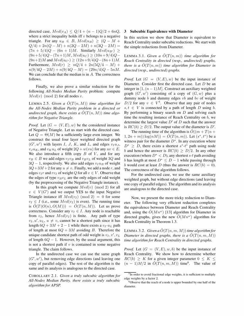
LEMMA 3.1. Given a O(T (n,m)) time algorithm forReach Centrality in directed (resp., undirected) graphs,there is a O(T (n,m)) time algorithm for Diameter indirected (resp., undirected) graphs.

Proof. Let (G = (V,E), w) be the input instance ofDiameter. Consider first the directed case. Let D be aninteger in [1, (n− 1)M ]. Construct an auxiliary weightedgraph (G′, w′) consisting of a copy of (G,w) plus adummy node b and dummy edges vb and bv of weightD/2 for any v ∈ V 5. Observe that any pair of nodess, t ∈ V is connected by a path of length D using b.By performing a binary search on D and solving eachtime the resulting instance of Reach Centrality on b, wedetermine the largest value D′ of D such that the answeris RC(b) ≥ D/2. The output value of the diameter is D′.

The running time of the algorithm is O((m+ T (n+1, 2n+m)) log(nM)) = O(T (n,m)). Let (s∗, t∗) be awitness pair for the diameter D∗. In any execution whereD∗ ≥ D, there exists a shortest s∗-t∗ path using nodeb and hence the answer is RC(b) ≥ D/2. In any otherexecution (whereD∗ < D), any shortest s-t path avoidingb has length at most D∗ ≤ D − 1 while passing throughb would cost at least D (thus the answer is RC(b) = 0).The correctness of the algorithm follows.

For the undirected case, we use the same auxiliaryweighted graph, but without edge directions (and leavingone copy of parallel edges). The algorithm and its analysisare analogous to the directed case.

Now, we present the more tricky reduction to Diam-eter. The following very efficient reduction completesthe equivalence between Diameter and Reach Centralityand, using the O(Mnω) [13] algorithm for Diameter indirected graphs, gives the new O(Mnω) algorithm forReach Centrality in Theorem 1.3.

LEMMA 3.2. Given a O(T (n,m,M)) time algorithm forDiameter in directed graphs, there is a O(T (n,m,M))time algorithm for Reach Centrality in directed graphs.

Proof. Let (G = (V,E), w, b) be the input instance ofReach Centrality. We show how to determine whetherRC(b) ≥ K for a given integer parameter 0 ≤ K ≤(n − 1)M/2 in O(T (n,m,M)) time6. The value of

5In order to avoid fractional edge weights, it is sufficient to multiplyedge weights by a factor 2.

6Observe that the reach of a node is upper bounded by one half of thediameter.

RC(b) can then be determined via binary search with anextra factor O(log(nM)) = O(1) in the running time.

Observe that, if the answer is YES, there must betwo nodes s, t ∈ V − b such that some shortest s-t path passes through b, K + M > d(s, b) ≥ K , andK + M > d(b, t) ≥ K . We construct an instance(G′, w′) of Diameter as follows. We add to G′ a copyof G. Furthermore, we add a set of nodes A that containsa node vA for each node v ∈ V such that K + M >d(v, b) ≥ K . Symmetrically, we add a set of nodes Bthat contains a node vB for each node v ∈ V such thatK + M > d(b, v) ≥ K . We also add edges vAv andvvB of weight K + M − d(v, b) and K + M − d(b, v),respectively. Note that the weight of the latter edges is in[1,M ] by construction. Finally, we add a directed pathP = v0, . . . , vq , q = ⌈(2K + 2M − 2)/M⌉, whoseedge weights are chosen arbitrarily in [1,M ] so that thelength of P is exactly 2K + 2M − 2. For every v ∈ V ,we add edges vv0 and vqv of weight zero. We also addedges av0 of weight 1 and vqa of weight 0 for any a ∈ A.Symmetrically, we add edges vqb of weight 1 and bv0 ofweight 0 for any b ∈ B.

We compute the diameter D∗ of (G′, w′) and outputthat RC(b) ≥ K iff D∗ ≥ 2K + 2M . The running timeof the algorithm is O(m + T (O(n), O(m + n),M)) =O(T (n,m,M)). Consider its correctness. The distancebetween any two nodes in G∪P is at most 2K+2M−2.The distance between any node in G ∪ P and any othernode is at most 2K + 2M − 1. The distance between anynode in B and any other node is at most 2K+2M−1. Thedistance between any node in A and any node in G∪P ∪Ais at most 2K + 2M − 1.

Consider next any pair sA ∈ A and tB ∈ B. An sA-tB path using P would cost at least 2K +2M . A shortestsA-tB path avoidingP costs 2K+2M−d(s, b)−d(b, t)+d(s, t) ≤ 2K+2M , where the equality holds iff b is alongsome shortest s-t path. Therefore D∗ ≤ 2K + 2M andthe equality holds iff there exists a pair (sA, tB) ∈ A×Bsuch that d(s, t) = d(s, b) + d(b, t), i.e. iff RC(b) ≥ K .The correctness follows.

Our subcubic reduction in the undirected case isslightly less efficient in terms of the edge weights and willfollow from Lemmas 4.2 and 4.3 of the next section.

4 Fast Approximation of Reach and BetweennessCentrality

In this section we present our results about the approx-imability of Reach and Betweenness Centrality. A keyidea in our approach is to consider the following PositiveBetweenness Centrality problem, which might be of in-dependent interest: determine whether BC(b) > 0 fora given node b (i.e., whether some shortest path uses bas an intermediate node). In this case it is convenient to

consider the standard definition of BC(b), where multipleshortest paths are allowed. Our results can be easily ex-tended to the case of unique shortest paths by perturbingweights by small polynomial factors.

Trivially, any α-approximation algorithm for Be-tweenness Centrality, for any finite α, also solves Pos-itive Betweenness Centrality since the answer is 0 iffBC(b) = 0. A similar reduction also works for ReachCentrality. In more detail, by definition RC(b) ≥mind(b, b), d(b, b) = 0 and RC(b) > 0 impliesBC(b) > 0. However, it might still be that RC(b) = 0and BC(b) > 0. We can solve this issue by initially per-turbing edge weights by small polynomial factors, so asto obtain an equivalent instance of Positive BetweennessCentrality where all weights are strictly positive. In thereduced instance RC(b) > 0 iff BC(b) > 0.

4.1 Some Results on Positive Betweenness Centrality.A simple observation is that on unweighted graphs,

Positive Betweenness Centrality is asking whether there isan in-neighbor x of b and an out-neighbor y of b such thatxy /∈ E, and therefore can be solved in O(m) time. Wenext show that, on weighted graphs, Positive BetweennessCentrality and Diameter are equivalent under subcubicreductions.

THEOREM 4.1. Diameter and Positive BetweennessCentrality are equivalent under subcubic reductions.

Theorem 4.1 follows from the following two lemmas.

LEMMA 4.1. Given a O(T (n,m)) time algorithm forPositive Betweenness Centrality in directed (resp., undi-rected) graphs, there is a O(T (n,m)) time algorithm forDiameter in directed (resp., undirected) graphs.

Proof. Let (G = (V,E), w) be the input instance ofDiameter. Consider first the directed case (see also Figure3). Let D be an integer in [1, (n − 1)M ]. Construct anauxiliary weighted graph (G′, w′) consisting of a copy of(G,w) plus a dummy node b and dummy edges vb and bvof weight D/2 for any v ∈ V 7. Observe that any pair ofnodes s, t ∈ V is connected by a path of length D using b.By performing a binary search onD and solving each timethe resulting instance of Positive Betweenness Centralityon b, we determine the largest value D′ of D such that theanswer is YES (i.e., BC(b) > 0). The output value of thediameter is D′.

The running time of the algorithm is O((m+ T (n+1, 2n+m)) log(nM)) = O(T (n,m)). Let (s∗, t∗) be awitness pair for the diameter D∗. In any execution whereD∗ ≥ D, there exists a shortest s∗-t∗ path using nodeb and hence the answer is YES. In any other execution

7In order to avoid fractional edge weights, it is sufficient to multiplyedge weights by a factor 2.

9

Figure 3 (Left) Reduction from Diameter to Positive Betweenness Centrality in directed graphs. Gray edges haveweight D/2, where D is a guess of the diameter. (Middle) Reduction from Positive Betweenness Centrality toDiameter in directed graphs. Here D is a proper upper bound on the diameter. (Right) Reduction from the NegativeTriangle instance of Figure 2 to All-Nodes Positive Betweenness Centrality in directed graphs (partially drawn). Grayedges have weight 3Q. One has BC(3B) > 0 and BC(0B) = 0 since node 3 does not belong to a negative trianglewhile node 0 does it.

0

1

2

b

2 3

3

4

b

1

2

bA

1A

2A

bB

1B

2B

2 3

3 4

0 0

D+1-3 D+1-2

D+1-4 0

3B

2B

1B

0B

3I

2I

1I

0I 0J

1J

2J

3J

0K

1K

2K

3K 3L

2L

1L

0L2Q-8

2Q+2

2Q+4

2Q

+6

2Q-8

2Q+4

(where D∗ < D), any shortest s-t path avoiding b haslength at most D∗ ≤ D−1while passing through b wouldcost at least D (thus the answer is NO). The correctnessof the algorithm follows.

For the undirected case, we use the same auxiliaryweighted graph, but without edge directions (and leavingone copy of parallel edges). The algorithm and its analysisare analogous to the directed case.

LEMMA 4.2. Given a O(T (n,m,M)) time algorithm forDiameter in directed (resp., undirected) graphs, there is aO(T (n,m,M)) time algorithm for Positive BetweennessCentrality in directed (resp., undirected) graphs.

Proof. Let (G,w, b) be the input instance of PositiveBetweenness Centrality. Observe that the answer is YESiff there exists a shortest path of the form s, b, t.

Let us consider the directed case first (see also Figure3). By adding a dummy node r and dummy edges vrand rv of weight M for any v ∈ V − b, we canassume that the diameter of G is at most D = 3M(w.l.o.g., b has at least one in-neighbor and one out-neighbor). Note that we did not introduce new paths ofthe form s, b, t. Furthermore, the new graph has n + 1nodes, m+ 2n edges, and maximum weight M . Hence aO(T (n,m,M)) time algorithm for the modified instanceimplies the same running time for the original one.

We construct an instance (G′, w′) of Diameter asfollows. Initially G′ = G. We add two copies A andB of V . Let vA be the copy of v ∈ V and define vBanalogously for B. For every v ∈ V , we add edges vAvand vvB of weight D + 1 − w(vb) and D + 1 − w(bv),respectively. If edges vb or bv are missing (includingthe case v = b), we set the weight of the correspondingedges vAv and vvB , respectively, to 0. Observe that edgeweights are O(M).

In this graph we compute the diameter D∗ and outputYES to the input Positive Betweenness Centrality instance

iff D∗ ≥ 2D + 2. The running time of the algorithmis O(m + T (O(n), O(m), O(M))) = O(T (n,m,M)).Consider a witness pair s∗, t∗ for the value of the diameter.Since edges of type vAv and vvB have positive weight,we can assume w.l.o.g. that s∗ = sA ∈ A and t∗ =tB ∈ B. If both edges sb and bt are missing, one hasD∗ = dG(s, t) ≤ D. If exactly one of the mentionededges is missing, say bt, one has D∗ = D+ 1−w(sb) +dG(s, t) ≤ 2D+1. Finally, if both edges are present, onehas D∗ = 2(D+1)−w(sb)−w(bt)+dG(s, t) ≤ 2D+2,where equality holds iff s, b, t is a shortest path. Inparticular, if there exists a shortest path of the mentionedtype, D∗ = 2D + 2 and otherwise D∗ ≤ 2D + 1. Thecorrectness follows.

By simply removing edge directions in the aboveconstruction, one obtains the claim in the undirected case.

We can exploit the above equivalence to derive (indi-rectly) the equivalence between Diameter and Reach Cen-trality in both directed and undirected graphs (recall thatwe showed this equivalence only in directed graphs).

LEMMA 4.3. Given a O(T (n,m)) time algorithm forPositive Betweenness Centrality in directed (resp., undi-rected) graphs, there is a O(T (n,m)) time algorithm forReach Centrality in directed (resp., undirected) graphs.

Proof. Let (G,w, b) be the input instance of Reach Cen-trality. We show how to determine whether RC(b) ≥ Kfor a given parameter K in O(T (n,m)) time. The valueof RC(b) can then be determined via binary search withan extra factor O(log(nM)) = O(1) in the running time.

Let us consider the directed case first. We computethe shortest path distances from and to b in G. Next weconstruct an auxiliary weighted graph (G′, w′) as follows.We let G′ initially contain a copy of G − b = G[V −b], plus an isolated node b. Next, for any v ∈ V − b,we add an edge vb of weight d(v, b) iff d(v, b) ≥ K .

Symmetrically, we add an edge bv of weight d(b, v) iffd(b, v) ≥ K .

We solve the Positive Betweenness Centrality in-stance (G′, w′, b) and output that RC(b) ≥ K iff theanswer is YES. The running time of the algorithm isO(m + T (n,m + 2n)) = O(T (n,m)). Let us prove itscorrectness. Suppose that RC(b) ≥ K and let (s, t) be awitness pair of that. Then s, b, t is a shortest s-t path inG′ and therefore the answer to the Positive BetweennessCentrality instance is YES. Vice versa, suppose that theanswer to the Positive Betweenness Centrality instance isYES, i.e. there exists a shortest s-t path passing throughb. This implies that there exists a shortest path of the forms′, b, t′. Observe that the shortest paths not involving nodeb are the same in G and G′. Therefore there exists a short-est s′-t′ path in G′ passing through b. Since by construc-tion dG(s′, b), dG(b, t′) ≥ K , the pair (s′, t′) witnessesthat RC(b) ≥ K .

The claim in the undirected case follows from thesame reduction, but removing edge directions (and leav-ing only one copy of parallel edges).

Another interesting observation about Positive Be-tweenness Centrality is that although solving it for a sin-gle node b is equivalent to Diameter under subcubic re-ductions, the all-nodes version of the problem (where onewants to determine whether BC(b) > 0 for all nodes b) isactually at least as hard as APSP.

LEMMA 4.4. Given a O(T (n,m,M)) time algorithmfor All-Nodes Positive Betweenness Centrality in directed(or undirected) graphs, there is a O(T (n,m,M)) timealgorithm for Negative Triangle.

Proof. Let (G,w) be the input instance of Negative Tri-angle. Consider first the directed case (see also Figure3). We create a directed weighted graph (G′, w′) as fol-lows. Graph G′ contains five copies I , J , K , L and B ofthe node set V . With the usual notation vX is the copyof node v ∈ V in set X . Let Q = Θ(M) be a suf-ficiently large integer. For every edge uv ∈ E we addthe edges uIvJ , uJvK , uKvL to G′ and set their weightto 2Q+w(uv). We also add edges uIuB and uBuL forevery node u in G and set the weight of these edges to3Q.

The algorithm solves the All-Nodes Positive Be-tweenness Centrality problem on (G′, w′) in timeO(T (n,m,M)), and outputs YES to the input NegativeTriangle instance iff BC(uB) > 0 for some uB ∈ B. Toshow correctness, observe that the only path through uB

is from uI to uL and it has weight 6Q, while every pathof type uI , vJ , wK , uL corresponds to a triangle u, v, win G and the weight of the path equals the weight of thetriangle plus 6Q. The claim follows.

The same construction, without edge directions,proves the claim for undirected graphs.

COROLLARY 4.1. Given a truly subcubic approximationalgorithm for All-Nodes Reach/Betweennees Centrality,there exists a truly subcubic algorithm for APSP.

4.2 A PTAS for Betweenness Centrality. In this sec-tion we prove the subcubic equivalence between Approx-imate Betweenness Centrality (for any constant approxi-mation factor α > 1) and Diameter.

THEOREM 4.2. Diameter and Approximate BetweennessCentrality are equivalent under subcubic Monte-Carloreductions.

Similarly to the case of Reach Centrality, it is not hardto see that a truly subcubic α-approximation algorithmfor Betweenness Centrality provides a truly subcubicalgorithm for Positive Betweenness Centrality (hence forDiameter via Theorem 4.1).

We next show that a truly subcubic algorithm forDiameter implies a truly subcubic PTAS for BetweennessCentrality, i.e. an algorithm that computes a (1 + ε)approximation of the betweenness centrality of a givennode for any given constant ε > 0. Our PTAS is Monte-Carlo: it provides the desired approximation w.h.p.

Let (G,w, b) be the considered instance of Between-ness Centrality, and define B∗ = BC(b). Observethat, under the assumption that shortest paths are unique,BCs,t(b) ∈ 0, 1 and therefore B∗ ∈ 0, . . . , (n −1)(n−2). Given s, t ∈ V −b such that BCs,t(b) = 1,we call (s, t) a witness pair, s a witness source, and t awitness target (of BC(b)).

Let also Bmed ∈ [0, (n − 1)(n − 2)] be a integerparameter to be fixed later. Our PTAS is based on twodifferent algorithms: one for B∗ ≤ Bmed and the otherfor B∗ > Bmed.

4.2.1 An exact algorithm for small B∗. Let us startwith the algorithm for small B∗. Recall that a witnesspair (s, t) satisfies BCs,t(b) = 1. A crucial observation isthat the number of witness pairs is equal to B∗ in case ofunique shortest paths.

It is convenient to define a generalization of Be-tweenness Centrality, where we consider only some pairs(s, t). For S, T ⊆ V − b, we define BCS,T (b) :=∑

(s,t)∈S×T BCs,t(b). The (S, T )-Betweenness Central-ity problem is to compute BCS,T (b). The Positive (S, T )-Betweenness Centrality problem is to determine whetherBCS,T (b) > 0. We use the shortcuts BCs,T (b) =BCs,T (b) and BCS,t(b) = BCS,t(b). Our first in-gredient is a reduction of that problem to Diameter.

LEMMA 4.5. Given a O(T (n,m)) time algorithm forDiameter in directed (resp., undirected) graphs, thereexists a O(T (n,m)) time algorithm for Positive (S, T )-Betweenness Centrality in directed (resp., undirected)graphs.

11

Proof. We use a construction similar to the one in theproof of Lemma 4.2. Let (G,w, b, S, T ) be the consideredinstance of Positive (S, T )-Betweenness Centrality. Westart with the directed case, the undirected one beinganalogous. Let us construct a directed weighted graph(G′, w′). Graph G′ contains a copy of G. Furthermore,it contains a copy of S and a copy of T . Let vS be thecopy of node v in S, and define vT analogously. LetK := 2 + A, where A is the maximum distance of typed(s, b) and d(b, t), with s ∈ S and t ∈ T . For eachs ∈ S and t ∈ T , we add edges sSs and ttT of weightK − d(s, b) and K − d(b, t), respectively. Observe thatthe latter weights are lower bounded by 2. We also addtwo nodes r′ and r′′, with an edge r′r′′ of weight 2. Weadd edges vr′ and r′v for every v ∈ V ∪ S of weightK − 1. Symmetrically, we add edges vr′′ and r′′v forevery v ∈ V ∪ T of weight K − 1. We also add edgesvr′ of weight K − 1 for every v ∈ T . We compute thediameter D∗ of (G′, w′), and output YES iff D∗ < 2K .

The running time of the algorithm is O(m +T (O(n), O(m))) = O(T (n,m)). Let us prove its cor-rectness. The distance from any node v ∈ V ∪T∪r′, r′′to any node w ∈ V ∪ S ∪ T ∪ r′, r′′ is at most2(K − 2). Consider next any node s ∈ S. Its distanceto any node in G ∪ r′, r′′ is also at most 2(K − 2).It remains to consider the distance from s to any t ∈ T .Any path using r′ or r′′ (or both) has length at least 2K .The shortest path avoiding r′ and r′′ has length precisely2K − d(s, b) − d(b, t) + d(s, t) ≤ 2K , where the equal-ity holds iff b belongs to some shortest s-t path. Wecan conclude that the diameter is smaller than 2K iff bis along some shortest s-t path with s ∈ S and t ∈ T ,i.e., iff the answer to the input instance of Positive (S, T )-Betweenness Centrality is YES.

The construction for the undirected case is similar,where we remove edge directions and also remove theedges of type vr′ with v ∈ T (those edges were neededonly to guarantee that distances from T to S are smallerthan 2K , while this property should not always hold in theundirected case). The running time remains O(T (n,m)).Analogously to the directed case, it is not hard to provethat pairwise distances are always smaller than 2K ex-cluding possibly the distance between some s ∈ S andt ∈ T which is equal to 2K iff b belongs to some shortests-t path. The correctness follows.

We will exploit the following recursive algorithm for(S, T )-Betweenness Centrality.

LEMMA 4.6. Given a O(T (n,m)) time algorithm forDiameter in directed (resp., undirected) graphs, there is aO(W · T (n,m)) time algorithm for (S, T )-BetweennessCentrality, where W is the number of pairs (s, t) ∈ S×Tsuch that BCs,t(b) = 1.

Proof. We describe a recursive algorithm with the

claimed running time, given a O(T (n,m)) time algorithmfor Positive (S, T )-Betweenness Centrality. The claimfollows from Lemma 4.5.

The recursive algorithm works as follows. It initiallysolve the corresponding Positive (S, T )-Betweenness in-stance. If the answer is NO, the algorithm outputs 0. Oth-erwise, if |S| = |T | = 1, the algorithm outputs 1. Other-wise, the algorithm partitions arbitrarily S into two sub-sets S1 and S2 of roughly the same cardinality, and it splitssimilarly T into T1 and T2. Then the algorithm solves re-cursively the sub-problems induces by the pairs (Si, Tj),i, j ∈ 1, 2, and outputs the sum of the four obtainedvalues.

The correctness of the algorithm is obvious. Con-cerning its running time, consider the recursion tree.Let us call a subproblem whose corresponding Positive(S, T )-Betweenness Centrality instance is a YES/NO in-stance a YES/NO subproblem. Observe that, excludingthe root problem, any NO subproblem must have at leastone sibling YES subproblem in the recursion tree. Fur-thermore, each sub-problem has at most 4 children in therecursion tree. Therefore, if the root subproblem is a YESsubproblem, the total number of subproblems is at most 4times the number of YES subproblems. Note also that thenumber of leaf YES subproblems is equal to W , and thateach YES subproblem must have at least one leaf YESsubproblem among its descendants. Finally, the depth ofthe recursion tree is O(log(|S|+ |T |)) = O(log n). Thusthe number of subproblems is O(W ). The claim on therunning time follows.

We are now ready to present our algorithm for smallB∗.

LEMMA 4.7. Given an instance (G,w, b) of BetweennessCentrality, a parameter Bmed, and an algorithm forDiameter of running time O(T (n,m)). There is anO(BmedT (n,m)) time algorithm which either outputsB∗ = BC(b) or answers NO in which case B∗ > Bmed.

Proof. Consider the recursive algorithm from Lemma4.6. We run that algorithm with S = T = V − b.Furthermore, we keep track of the number W of leaf YESsub-problems found so far. If W > Bmed at any point, wehalt the recursive algorithm and output NO. Otherwise,we output the value W returned by the root call of therecursive algorithm.

The correctness of the algorithm follows immediatelysince the number of leaf YES subproblems in the original(non-truncated) algorithm equals B∗. An easy adaptationof the running time analysis in Lemma 4.6 shows that therunning time is as in the claim.

4.2.2 A Monte-Carlo PTAS for large B∗. We nextassume that B∗ > Bmed, and we present an algorithm

for this case. In order to lighten the notation, we nextdrop b (which is clear from the context). Recall thata node w is a witness source (resp., witness target) ifBCw,V > 0 (resp., BCV,w > 0). At high level, ouralgorithm is based on the computation of the contributionBCs,V to BC of a random sample of candidate witnesssources s. Then we exploit Chernoff’s bound to prove thatthe approximation factor is small w.h.p. One technicaldifficulty here is that some witness sources might give avery large contribution to BC, which is problematic sincewe need concentrated results. In order to circumvent thisproblem, we first sample a random subset of candidatewitness targets to identify the problematic witness sources(which are considered separately).

In more detail, we sample a random subset T ofpmed · n nodes, where pmed = C logn√

Bmedand C is a

sufficiently large constant. We compute all the shortestpaths ending in T , and use them to derive BCs,T for alls ∈ V . We partition V into sets Slarge and Ssmall, wheres ∈ V belongs to Slarge iff BCs,T ≥ C logn. Then wesample a random subset Rsmall of pmed|Ssmall| nodes inSsmall, and compute BCs,V for all s ∈ Rsmall. Finally,we output the estimate

B =1

pmed(∑

s∈Slarge

BCs,T +∑

s∈Rsmall

BCs,V ).

It is easy to see that the running time of the algo-rithm is O( nm√

Bmed). It is also not hard to see that

E[ 1pmed

∑s∈Slarge

BCs,T ] =∑

s∈SlargeBCs,V and

E[ 1pmed

∑s∈Rsmall

BCs,V ] =∑

s∈SsmallBCs,V . There-

fore, E[B] = B∗. The following lemma shows that B isconcentrated around its mean.

LEMMA 4.8. W.h.p. B ∈ [(1 − 2ε)B∗, (1 + 2ε)B∗],where ε > 0 tends to zero as C tends to +∞.

Proof. We start by showing that w.h.p., for any s ∈ V , ifs ∈ Slarge then BCs,V ≥

√Bmed/(1+ε), and otherwise

BCs,V ≤√Bmed/(1 − ε). Define B′ = BCs,T and

B = BCs,V . Note that E[B′] = C log n√Bmed

B. Note also thatB′ = BCs,T =

∑t∈V Xs,t, where Xs,t = 0 if t /∈ T

and Xs,t = BCs,t otherwise. Since the variables Xs,t arenegatively correlated, we can apply Chernoff’s bound toBCs,T . In particular, conditioning on B <

√Bmed

1+ε , oneobtains

Pr[B′ ≥ C logn =

√Bmed

BE[B′]]

≤(

e(√Bmed/B)−1

(√Bmed/B)

√Bmed/B

) C log n√Bmed

B

≤(eε/(1+ε)

1 + ε

)C logn

.

Above we used the fact that function xe1−x is increasingfor x ∈ [0, 1

1+ε ] (and strictly smaller than 1 in the samerange). Similarly, conditioning on the event that B >√

Bmed

1−ε , one obtains E[B′] = C logn√Bmed

B ≥ C logn1−ε and

Pr[B′ < C log n =

√Bmed

BE[B′]]

≤ Pr[B′ ≤ (1− ε)E[B′]]

≤ e−ε2E[B′]

2 ≤ e−ε2C log n2(1−ε) .

The claim follows from the union bound for C largeenough.

Next assume that the mentioned high probabilityevent happens for all s ∈ V . Define B∗

large =∑s∈Slarge

BCs,V and B∗small =

∑s∈Ssmall

BCs,V .Clearly B∗ = B∗

large + B∗small. Define also

Blarge := 1pmed

∑s∈Slarge

BCs,T and Bsmall :=1

pmed

∑s∈Rsmall

BCs,V , so that B = Blarge + Bsmall.Consider any s ∈ Slarge, and define B′ = BCs,T

and B = BCs,V . Recall that by assumption B ≥√Bmed

1+ε

and observe that E[B′] = pmedB ≥ C log n1+ε . Then, by

Chernoff’s bound,

Pr[|B′ − E[B′]| ≥ εE[B′]]

≤ 2e−ε2

3 E[B′] ≤ 2e−ε2

3(1+ε)C logn.

Since E[Blarge] = 1pmed

[∑

s∈SlargeBCs,T ] = B∗

large,we can conclude that w.h.p. Blarge ∈ [(1−ε)B∗

large, (1+ε)B∗

large].Consider next Bsmall. Define B′ = pmedBsmall =∑

s∈RsmallBCs,V . Observe that E[B′] = pmedB∗

small.Furthermore B′ is the sum of independent random vari-ables each one of value at most

√Bmed

1−ε by the assumptionon Ssmall. Therefore, by Chernoff’s bound,

Pr[B′ ≥ E[B′] + εpmedB∗]

≤

⎛

⎜⎝e

εB∗B∗

small

( εB∗

B∗small

+ 1)εB∗

B∗small

+1

⎞

⎟⎠

(1−ε)C log nB∗small

Bmed

.

Assuming B∗small ≥ εBmed/2 and observing that B∗ ≥

B∗small, one obtains

Pr[B′ ≥ E[B′] + εpmedB∗]

≤(

eε

(1 + ε)1+ε

) (1−ε)εC log n2

.

13

Otherwise B∗small < εBmed/2 ≤ εB∗/2 and thus

Pr[B′ ≥ E[B′] + εpmedB∗]

≤

⎛

⎝ eε

(1 + εB∗

B∗small

)B∗

smallB∗ +ε

⎞

⎠

(1−ε)C log nB∗Bmed

≤(e3

)ε(1−ε)C logn.

Similarly

Pr[B′ ≤ E[B′]− εpmedB∗]

≤ e− 1

2 (εB∗

B∗small

)2pmedB∗

small√Bmed/(1−ε)

= e− (1−ε)ε2

2(B∗)2

B∗small

C log nBmed

≤ e−(1−ε)ε2

2 C logn.

Therefore w.h.p. Bsmall ∈ [B∗small−εB∗, B∗

small+εB∗].Altogether, w.h.p. one has

(1 − 2ε)B∗ ≤ (1− ε)B∗large +B∗

small − εB∗ ≤ B

≤ (1 + ε)B∗large +B∗

small + εB∗ ≤ (1 + 2ε)B∗.

The following lemma summarizes the above discus-sion.

LEMMA 4.9. Given an instance (G,w, b) of Between-ness Centrality with BC(b) = B∗ ≥ Bmed, there is anO( nm√

Bmed) time algorithm that returns a (1 + ε) approxi-

mation of B∗ w.h.p.

Combining the algorithms for small and large B∗, weobtain the following result.

LEMMA 4.10. Given a truly subcubic algorithm for Di-ameter, there exists a truly subcubic Monte-Carlo PTASfor Betweenness Centrality.

Proof. Let O(n3−δ) be the running time of the givenDiameter algorithm, for some constant δ > 0. FromLemmas 4.7 and 4.9, we can use it to compute w.h.p. a(1 + ε) approximation of the betweenness centrality of agiven node in time O(Bmedn3−δ + n3

√Bmed

). ChoosingBmed = n2δ/3 gives a truly subcubic running time inO(n3−δ/3).

Theorem 4.2 follows directly from Lemma 4.10.

4.3 Reductions based on SETH. We are able to showthat, assuming the Strong Exponential Time Hypothesis(SETH) [33], a subquadratic algorithm for Positive Be-tweenness Centrality does not exist even in sparse graphs.We recall that SETH claims that CNF-SAT on n variables

cannot be solved in time O((2 − δ)n) for any constantδ > 0. By the same observation as before, one obtains asa corollary a lower bound on the running time of any ap-proximation algorithm for Betweenness/Reach Centrality.

THEOREM 4.3. Suppose that there is an O(m2−ε) timealgorithm, for any constant ε > 0, that solves PositiveBetweenness Centrality in directed or undirected graphswith edge weights in 1, 2. Then SETH is false.

Proof. Let F be a CNF-SAT formula on n variables.Our goal is to show that we can determine whether F issatisfiable in O∗(2(1−δ)n) time for some constant δ > 08.Using the sparsification lemma of [33] (as, e.g., in [10]),we can assume w.l.o.g. that F contains O(n) clauses.

Let us consider the undirected case first (see alsoFigure 4). We partition the variables into two sets Aand B of (roughly) n/2 variables each, and create a nodefor each partial assignment of the variables in A and B,respectively. We also add a node for each clause c, andadd one edge of weight 1 between each clause c and anypartial assignment φ of A or B that does not satisfy anyliteral of c (including the special case that c does notcontain any variable in A or B). We also add two nodesxA and xB , and add one edge of weight 1 between themand any node in A and B, respectively. Finally we add anode b, and add one edge of weight 2 between b and anyassignment of A and B.

We claim that F is satisfiable iff BC(b) > 0.Observe that the distance between any clause node cand any other node is at most 4, while any path passingthrough b would cost at least 5. Similarly, the distancebetween any two assignment of A or of B is at most 2,so the corresponding shortest paths do not use b. Givenan assignment φA of A and an assignment φB of B, thereexists a φA-φB path of length 2 (hence BCφA,φB (b) = 0)iff there exists a clause c that is not satisfied by φA norby φB . Otherwise (i.e., φA and φB together satisfy F ),φA, b,φB is a a shortest such path (hence BC(b) > 0).The graph has O(2n/2n) edges, and the conclusion of thelemma follows.

In the directed case we can use a similar construction,without nodes xA and xB , and orienting the edges fromthe assignments of A to the clause nodes and to b, andfrom the latter nodes to the assignments of B. Thealgorithm and its analysis are analogous to the undirectedcase.

COROLLARY 4.2. Suppose that there is an O(m2−ε)time α-approximation algorithm for Betweenness Cen-trality or Reach Centrality, for any constant ε > 0 andany finite α (possibly depending on m). Then SETH isfalse.

8The O∗ notation suppresses polynomial factors.

Figure 4 Reduction from CNF-SAT to Positive Betweenness Centrality (left) and Reach Centrality (right) in undirectedgraphs for the CNF-SAT formula c1∧ c2 ∧ c3∧ c4 = (X ∨Y ∨Z)∧ (Z ∨Y )∧ (X ∨Y ∨Q)∧ (X ∨Z ∨Q). The set ofvariables are A = X,Y and B = Z,Q. Node AFF corresponds to the partial assignment (X,Y ) = (F, F ) andsimilarly for the other nodes. Bold edges have weight 2, all other edges have weight 1. The shortest paths AFF , r, BTT

on the left and AFF , xA, r, xB , BTT on the right witness that (X,Y, Z,Q) = (F, F, T, T ) is a satisfying assignment.

AFF ATF AFT ATT

c1 c2 c4c3

BFF BTF BFT BTT

xA

xB

r

AFF ATF AFT ATT

c1 c2 c4c3

BFF BTF BFT BTT

xA

xB

r

For Reach Centrality we can also show an approxi-mation lower bound for unweighted undirected graphs.

THEOREM 4.4. Suppose there is a O(m2−ε)-time (2 −ε)-approximation algorithm for Reach Centrality in undi-rected unweighted graphs, for some constant ε > 0. ThenSETH is false.

Proof. Similarly to the proof of Theorem 4.3, we canstart with a CNF-SAT formula F containing n variablesand m = O(n) clauses [33]. We will show how toconstruct an instance (G, b) of Reach Centrality on anunweighted undirected graph G = (V,E) with |V | =O(2n/2 + m) nodes and |E| = O(2n/2m) edges, suchthat RC(b) = 2 if F is satisfiable and RC(b) = 1otherwise. The generation of the graph from the formulatakes O(2n/2m) time and therefore if we could computea (2 − ε) approximation of RC(b) in O∗(|E|2−ε) time,for some ε > 0, we would be able to solve CNF-SAT inO∗(2(1−ε/2)n) time (which would refute SETH).

Similarly to the proof of Theorem 4.3, we partitionthe variables into two subsets A and B of (roughly)n/2 variables each, and create a node for each partialassignment of the variables in A and B. We also createa node c for each clause c, and connect c to each partialassignment that does not satisfy any literal in c. We alsoadd nodes xA and xB , and add edges between them andany node in A and B, respectively. Finally, we add a nodeb, and connect it to xA and xB (note that the final part ofthe construction deviates from Theorem 4.3).

To show correctness, note that b is on the shortest pathbetween xA and xB and therefore RC(b) ≥ 1. Second,note that b cannot be on the shortest path between a clausenode c and another node in G, and therefore RC(b)= 2 if

and only if b is on the shortest path between an assignmentφA of A and an assignment φB of B. But a shortest pathbetween φA and φB goes through b if and only if for everyclause node c either φAc is not an edge or φBc is not anedge, and by definition of these edges it implies that forevery clause c, either φA or φB satisfies c (i.e. φA and φB

induce a satisfying assignment of F ). The claim follows.

5 Conclusions and Open ProblemsThere are many interesting problems that we left open.The main one is probably whether Diameter and APSP areequivalent under subcubic reductions. By our reductions,on one hand a positive answer would indicate that trulysubcubic algorithms for Reach Centrality and for Approx-imate Betweenness Centrality are unlikely to exist. On theother hand, a negative answer would give truly subcubicalgorithms for the latter problems as well.

We have shown that Reach Centrality can be solvedin O(Mnω) time in directed graphs, improving on theprevious best algorithm based on APSP. Similar runningtimes are known for Diameter and Radius [13]. To thebest of our knowledge, it is open whether a O(Mnω)time algorithm exists also for Median and BetweennessCentrality in directed graphs.

We proved that a subquadratic 2−ε approximation al-gorithm for Reach Centrality in sparse graphs is unlikelyto exist. In [45] an analogous result is proved for Diam-eter. It would be interesting to show similar negative re-sults for Radius, Betweenness Centrality and Median (orfind faster approximation algorithms in sparse graphs forthose problems).

References

15

[1] A. Abboud and V. V. Williams. Popular conjectures implystrong lower bounds for dynamic problems. FOCS, 2014.

[2] A. Abboud, V. V. Williams, and O. Weimann. Conse-quences of faster alignment of sequences. In ICALP (1),pages 39–51, 2014.

[3] D. Aingworth, C. Chekuri, P. Indyk, and R. Motwani.Fast estimation of diameter and shortest paths (withoutmatrix multiplication). SIAM J. Comput., 28(4):1167–1181, 1999.

[4] D. A. Bader, S. Kintali, K. Madduri, and M. Mihail.Approximating betweenness centrality. In WAW, pages124–137, 2007.

[5] P. Berman and S. P. Kasiviswanathan. Faster approxima-tion of distances in graphs. In WADS, pages 541–552,2007.

[6] U. Brandes. A faster algorithm for betweenness centrality.Journal of Mathematical Sociology, 25(2):163–177, 2001.

[7] U. Brandes and C. Pich. Centrality estimation in largenetworks. International Journal of Bifurcation and Chaos,17(7):2303–2318, 2007.

[8] T. M. Chan. More algorithms for all-pairs shortest pathsin weighted graphs. SIAM J. Comput., 39(5):2075–2089,2010.

[9] C.-L. Chang. Deterministic sublinear-time approxima-tions for metric 1-median selection. Inf. Process. Lett.,113(8), 2013.

[10] S. Chechik, D. Larkin, L. Roditty, G. Schoenebeck, R. E.Tarjan, and V. V. Williams. Better approximation algo-rithms for the graph diameter. In SODA, pages 1041–1052,2014.

[11] T. Coffman, S. Greenblatt, and S. Marcus. Graph-basedtechnologies for intelligence analysis. Communications ofthe ACM, 47(3):45–47, 2004.

[12] D. Coppersmith and S. Winograd. Matrix multiplicationvia arithmetic progressions. J. Symbolic Computation,9(3):251–280, 1990.

[13] M. Cygan, H. N. Gabow, and P. Sankowski. Algorithmicapplications of Baur-Strassen’s theorem: Shortest cycles,diameter and matchings. In FOCS, pages 531–540, 2012.

[14] A. Davie and A. J. Stothers. Improved bound for com-plexity of matrix multiplication. Proceedings of the RoyalSociety of Edinburgh, Section: A Mathematics, 143:351–369, 4 2013.

[15] A. Del Sol, H. Fujihashi, and P. O’Meara. Topology ofsmall-world networks of protein- protein complex struc-tures. Bioinformatics, 21(8):1311–1315, 2005.

[16] E. W. Dijkstra. A note on two problems in connexion withgraphs. Numerische Mathematik, 1:269–271, 1959.

[17] D. Eppstein and J. Wang. Fast approximation of centrality.J. Graph Algorithms Appl., 8:39–45, 2004.

[18] M. L. Fredman. New bounds on the complexity of theshortest path problem. SIAM J. Comput., 5(1):83–89,1976.

[19] M. L. Fredman and R. E. Tarjan. Fibonacci heaps andtheir uses in improved network optimization algorithms.J. ACM, 34(3):596–615, 1987.

[20] L. Freeman. A set of measures of centrality based uponbetweenness. Sociometry, 40:35–41, 1977.

[21] A. Gajentaan and M. Overmars. On a class of o(n2) prob-

lems in computational geometry. Computational Geome-try, 5(3):165–185, 1995.

[22] F. L. Gall. Powers of tensors and fast matrix multiplica-tion. In International Symposium on Symbolic and Alge-braic Computation, ISSAC ’14, Kobe, Japan, July 23-25,2014, pages 296–303, 2014.

[23] R. Geisberger, P. Sanders, and D. Schultes. Better approx-imation of betweenness centrality. In ALENEX, pages 90–100, 2008.

[24] A. V. Goldberg, H. Kaplan, and R. F. Werneck. Reach forA*: Efficient point-to-point shortest path algorithms. InALENEX, pages 129–143, 2006.

[25] A. V. Goldberg, H. Kaplan, and R. F. F. Werneck. Betterlandmarks within reach. In WEA, pages 38–51, 2007.

[26] O. Goldreich and D. Ron. Approximating average param-eters of graphs. Random Struct. Algorithms, 32(4):473–493, 2008.

[27] F. Grandoni and V. Vassilevska Williams. Improved dis-tance sensitivity oracles via fast single-source replacementpaths. In FOCS, pages 748–757, 2012.

[28] R. J. Gutman. Reach-based routing: A new approach toshortest path algorithms optimized for road networks. InALENEX/ANALC, pages 100–111, 2004.

[29] P. Hage and F. Harary. Eccentricity and centrality innetworks. Social Networks, 17:57–63, 1995.

[30] S. L. Hakimi. Optimum locations of switching centers andthe absolute centers and medians of a graph. Operationsresearch, 12(3):450–459, 1964.

[31] Y. Han and T. Takaoka. An O(n3 log log n/ log2 n) timealgorithm for all pairs shortest paths. In SWAT, pages 131–141, 2012.

[32] X. Huang and V. Y. Pan. Fast rectangular matrix multi-plication and applications. J. Complexity, 14(2):257–299,1998.

[33] R. Impagliazzo, R. Paturi, and F. Zane. Which problemshave strongly exponential complexity? J. Comput. Syst.Sci., 63(4):512–530, 2001.

[34] P. Indyk. Sublinear time algorithms for metric spaceproblems. In STOC, pages 428–434, 1999.

[35] H. Jeong, S. Mason, A. Barabasi, and Z. Oltvai. Lethalityand centrality in protein networks. Nature, 411:41–42,2001.

[36] D. B. Johnson. Efficient algorithms for shortest paths insparse networks. J. ACM, 24(1):1–13, 1977.

[37] V. Krebs. Mapping networks of terrorist cells. Connec-tions, 24(3):43–52, 2002.

[38] F. Liljeros, C. Edling, L. Amaral, H. Stanley, and Y. Aberg.The web of human sexual contacts. Nature, 411:907–908,2001.

[39] K. Mulmuley, U. V. Vazirani, and V. V. Vazirani. Matchingis as easy as matrix inversion. Combinatorica, 7(1):105–113, 1987.

[40] M. E. J. Newman and M. Girvan. Finding and evaluatingcommunity structure in networks. Physical Review E,69(2):26–113, 2004.

[41] S. Pettie. A new approach to all-pairs shortest paths onreal-weighted graphs. Theor. Comput. Sci., 312(1):47–74,2004.

[42] S. Pettie and V. Ramachandran. A shortest path algorithm

for real-weighted undirected graphs. SIAM J. Comput.,34(6):1398–1431, 2005.

[43] J. W. Pinney and D. R. Westhead. Betweenness-based de-composition methods for social and biological networks.In Interdisciplinary Statistics and Bioinformatics, pages87–90, 2006.

[44] M. Patrascu. Towards polynomial lower bounds for dy-namic problems. In STOC, pages 603–610, 2010.

[45] L. Roditty and V. Vassilevska Williams. Fast approxi-mation algorithms for the diameter and radius of sparsegraphs. In STOC, pages 515–524, 2013.

[46] L. Roditty and U. Zwick. Replacement paths and ksimple shortest paths in unweighted directed graphs. ACMTransactions on Algorithms, 8(4):33, 2012.

[47] G. Sabidussi. The centrality index of a graph. Psychome-tirka, 31:581–606, 1966.

[48] D. Schultes and P. Sanders. Dynamic highway-noderouting. In WEA, pages 66–79, 2007.

[49] A. Shoshan and U. Zwick. All pairs shortest paths inundirected graphs with integer weights. In FOCS, pages605–615, 1999.

[50] M. Thorup. Undirected single source shortest path inlinear time. In FOCS, pages 12–21, 1997.

[51] V. Vassilevska Williams. Faster replacement paths. InSODA, pages 1337–1346, 2011.

[52] V. Vassilevska Williams. Multiplying matrices faster thanCoppersmith-Winograd. In STOC, pages 887–898, 2012.

[53] V. Vassilevska Williams and R. Williams. Subcubic equiv-alences between path, matrix and triangle problems. InFOCS, pages 645–654, 2010.

[54] O. Weimann and R. Yuster. Replacement paths anddistance sensitivity oracles via fast matrix multiplication.ACM Transactions on Algorithms, 9(2):14, 2013.

[55] R. Williams. Faster all-pairs shortest paths via circuitcomplexity. In STOC, 2014.

[56] U. Zwick. All pairs shortest paths in weighted directedgraphs − exact and almost exact algorithms. In FOCS,pages 310–319, 1998.

[57] U. Zwick. All pairs shortest paths using bridging setsand rectangular matrix multiplication. J. ACM, 49(3):289–317, 2002.

17