Subaqueous barchan dunes in turbulent shear ow. Part 1 ...franklin/images/franklin_charru(2011).pdf · Subaqueous barchan dunes in turbulent shear ... By E.M. FRANKLIN AND F. CHARRU

Under consideration for publication in J. Fluid Mech. 1

Subaqueous barchan dunes in turbulentshear flow. Part 1: Dune motion

By E. M. F R A N K L I N AND F. C H A R R UInstitut de Mecanique des Fluides de Toulouse - CNRS–Universite de Toulouse -

Allee C. Soula, 31400 Toulouse, France.

(Received ?? and in revised form ??)

Experiments are reported on the formation and migration of isolated dunes in a turbulentchannel flow. These dunes have a very robust crescentic shape with horns pointing down-stream, very similar to that of the barchan dunes observed in deserts at a much largerscale. Their main geometrical and dynamical properties are studied in detail, for fourtypes of grains: the conditions for their formation, their morphology, the threshold shearstress for their motion, their velocity, erosion rate, minimum size, and the longitudinalstripes of grains hollowed by fluid streaks in the boundary layer. In particular, the law forthe dune velocity is found to involve two dimensionless parameters, the Shields numberand the sedimentation Reynolds number, in contrast with predictions based on classicallaws for particle transport. As the dune migrates, its size slowly decreases because ofa small leakage of particles at the horn tips, and the erosion law is given. A minimumsize is evidenced, which is shown to increase with the friction velocity and scale with asettling length.

1. IntroductionWhen sand grains are entrained by an air flow over a non-erodible ground, or with

limited sediment supply from the bed, they form dunes showing a remarkable crescen-tic shape with horns pointing downstream. These dunes, known as barchan dunes, arecommonly observed in deserts, with height of a few meters and velocity of a few tensof meters per year. In his famous book, Bagnold (1941) first pointed out their signifi-cance for understanding the physics of blown sand. Their outstanding shape and stabilityproperties have triggered a number of studies, aiming at understanding the conditionsfor their formation, their migration velocity and time evolution, and also the strikingexistence of a minimum length, of about ten meters, below which no dune is observed. Amodel accounting for their main properties was derived by Kroy, Sauermann & Hermann(2002) and Andreotti, Claudin & Douady (2002a, 2002b), from calculations of the shearstress at the dune surface by Hunt, Leibovich & Richards (1988) and a relaxation equa-tion for the sand flux accounting for the retarding effect of grain inertia (Sauermann,Kroy & Hermann 2001).

Similar barchan dunes have also been observed under water flows, with, however,much shorter lengths than in air, when, again, the sediment supply is limited. Suchdunes formed in an open channel flow are reported by Mantz (1978), with typical widthof about three centimeters (Figure 1a); in this paper the resemblance with the aeoliandunes observed by Bagnold was noted. This resemblance was investigated further byHersen, Douady & Andreotti (2002) and Hersen (2005) from experiments in which thedunes were formed on a tray oscillating asymmetrically in a water tank. Barchan dunes

2 E. M. Franklin and F. Charru

(a)

(b) (c)

Figure 1. Subaqueous barchan dunes. (a), in an open channel (Mantz 1978); (b) in a pipe(Al-lababidi et al. 2008); (c), in a closed channel from the present experiments, top and sideviews, and definition of the characteristic lengths (zircone beads with diameter d = 0.2 mm,dune length L = 50 mm). Water flows from left to right.

formed in a circular pipe are also clearly visible in a photograph shown by Al-lababidi etal. (2008) (Figure 1b); although this paper does not comment on their particular shape,it discusses the increase of the pressure drop and potential damages that isolated dunesmay cause in industrial pipe flows.

Barchan dunes under water have received much less attention than aeolian dunes,and important issues related to their dynamics remain unanswered. These issues are(i) the conditions under which barchan dunes form and disappear, and their migrationvelocity; (ii) the distributions of fluid velocity and shear stress over the dune surface,and the resulting particle flux; (iii) their stability properties and interactions in a field:splitting and merging of dunes of different size and velocity, existence of an eventualstable equilibrium size. This paper aims at answering these questions, from experimentsin a turbulent channel flow. The present Part One is devoted to the first issue of theformation and velocity of dunes; the following Part Two will deal with the second issueof the fluid motion near the dune. In this Part One, the experimental set-up and turbulentwater flow are described in §2. The formation, morphology and migration velocity of thebarchan dunes are analysed in §3. The results are summarized and discussed in §4.

Subaqueous barchan dunes in turbulent shear flow 3

Figure 2. Sketch of the experimental arrangement. (a), side-view; (b), cross-section of thechannel.

2. Experimental arrangement and channel flow2.1. Experimental arrangement

The experimental arrangement mainly consists of a horizontal plexiglass channel, sixmeters long, with rectangular cross-section of height 2δ = 60 mm and width b = 120mm (Figure 2a). Water flows from a head-tank with free surface 2.5 meters above thechannel, and enters the channel through a divergent-convergent device with a honeycombsection in order to suppress large eddies and homogeneize the small-scale turbulence. Atthe open end of the channel, particles are separated by sedimentation in a large tank,and a pump drives the water up to the head-tank. The volumetric flow rate is measuredwith an electromagnetic flow-meter.

The particles were deposited in the channel, previously filled with water, with the helpof a syringe through a small hole in the upper wall located at 4.15 m form the entrance.The sand settled in the water at rest and formed a conical heap. Then the flow wasstarted up, and the heap deformed into a barchan dune. The evolution of the shape ofthe dune was recorded with a video camera placed above the channel and mounted on atravelling system. The resolution of the camera was 2048×2048 pixels, with field of viewat the bottom wall of about 140× 140 mm2. The side view of the dune was recorded onthe same images thanks to a mirror inclined at 45◦, as shown in Figure 2b. A sample ofthe resulting image is shown in Figure 1c.

Fluid velocity measurements were performed in the vertical mid-plane of the channelusing Particle Image Velocimetry (PIV), as sketched in Figure 2b. A vertical laser sheet ofthickness of 1 mm was generated by a 30mJ Nd:Yag double-pulse laser, and illuminatedfluorescent rhodamine encapsulated in small acrylic beads, of density 1110 kg m−3 anddiameter of about 10 µm. A 1280 × 1024 px 12-bit CCD camera was used to capturethe images, with a 50 mm or 60 mm Nikon lens. The time interval between the twoimages of a pair was in the range 224–848 µs, and the sampling frequency of the pairs


were in the range 1–4 Hz. A high-pass filter interposed between the laser sheet and thecamera allowed suppression of the light scattered by the dunes and channel walls. Forflow measurements over the whole channel height, the field of view was 85 × 68 mm2,whereas for closer inspection near the dune, a smaller field of view was used, of 22× 17mm2. The PIV images were processed with the software PIVIS developed at IMFT, withcorrelation boxes of 16×16 pixels with sub-pixel accuracy; the resulting spatial resolutionof the velocity field was 1 mm with the large field, and 0.15 mm with the small one (inthe latter case an overlap of 50% of the correlation boxes was used). Convergence of thetime-averaged longitudinal and vertical velocities, U and V , was achieved within 1% withabout 30 frames, whereas a larger number, of about 200, was required for the Reynoldsstresses u′2, v′2 and u′v′.

2.2. Channel flowThe flow velocity 〈U〉, defined as the ratio of the measured volumetric flow rate andthe channel cross-section, was varied between 0.15 and 0.4 m s−1. The correspondingReynolds number

Re =〈U〉2δν

(2.1)

was in the range 9000− 24000, so that the flow was turbulent.Figure 3a displays mean velocity profiles U(y) in the mid-plane, four meters down-

stream of the inlet, for six Reynolds numbers in the range 14000–21000. The profilesappear to be symmetric with respect to the horizontal mid-plane, as expected. Thedepth-averaged velocity is slightly larger than the flow velocity 〈U〉, by about 4%, whichdifference corresponds to the retarding effect of the lateral walls. Plotting these veloci-ties with semi-logarithmic scales (not shown) reveals log-regions spanning approximatelyfrom 2 to 10 mm from the walls, allowing the friction velocity u∗ to be determined bylinear regression with κ = 0.41 for the Karman coefficient. Figure 3b displays the velocityprofiles in the lower half of the channel in wall units, U+ = U/u∗ versus y+ = yu∗/ν, forsix Reynolds numbers. It appears that for y+ in the range 30–200, data points collapseonto the same curve

U+ =1κ

ln y+ +B, (2.2)

with the coefficients κ = 0.41 and B = 5.5 having their usual values (Davidson 2004).Note that these coefficients have been shown to decrease slightly with Reynolds numberand reach constant values for large Reynolds number only (Nagib & Chauhan 2008); thesesmall variations have not been taken into account here. A slow secondary flow normal tothe main flow is known to develop in rectangular ducts, with typical velocity of about1% of the mean longitudinal velocity (Melling & Whitelaw 1976). This secondary flow isexpected to have negligible effect on the motion of dunes, and has not been measured.

Figure 4 shows the variation of the friction coefficient cf = u2∗/

12 〈U〉2 with Reynolds

number, together with the Blasius correlation

cf = 0.079 (1.33Re)−1/4. (2.3)

In this equation, the factor 1.33 arises because the Reynolds number involved in theBlasius correlation is based on the hydraulic diameter, and the friction velocity representsthe average over the perimeter of the channel (Schlichting 1979). It appears from Figure4 that the Blasius correlation provides a good fit of the measured friction velocities.

Figure 5a displays profiles of the Reynolds stress −u′v′, normalized by u2∗. This stress is

antisymmetric and varies linearly in the middle of the channel, as expected in a pressure-driven channel flow. Its maximum is slightly lower than u2

∗ and located at y/δ ≈ 0.2; closer


0 0.1 0.2 0.3 0.40

10

20

30

40

50

60

U (m/s)

y (m

m)

101 102 10310

12

14

16

18

20

22

y+

U+

(a) (b)

Figure 3. Velocity profiles U(y) in the vertical mid-plane of the channel for Re = 13900 (∗),15000 (�), 16200 (◦), 17400 (4), 18500 (O) and 19700 (�); (a), in linear dimensional scales; (b)in semilog wall scales in the lower half of the channel, with the straight line corresponding toequation (2.2).

1 1.5 2x 104

0

0.002

0.004

0.006

0.008

0.01

Re

cf

Figure 4. (◦), Friction coefficient versus Reynolds number; (—), Blasius correlation (2.3).

to the walls where viscous effects are no longer negligible, it decreases to zero. Figure5b displays the same profiles in wall units, magnifying the region close to the maximum;this plot confirms that stresses are nearly uniform in the region 30 < y+ < 200 wherethe log-law holds.

The Reynolds stresses u′2 and v′2, not shown, have also been determined and theirprofiles agree with those shown in the literature (Davidson 2004). In particular, u′2 isminimum and about u2

∗ at mid-height (y/δ = 1), it increases towards the walls andreaches a maximum of about 4–5u2

∗ in the log-region; similarly, v′2 is minimum and


!1 0 10

0.2

0.4

0.6

0.8

1

!u !v !/u 2"

y/2!

!1 0 10

50

100

150

200

250

300

!u !v !/u 2"

y+

(a) (b)

Figure 5. Vertical profiles of the normalized Reynolds stresses −u′v′/u2∗ for the same Reynolds

numbers as in Figure 3 ; (a), over the whole channel height; (b), close to the bottom wall in wallunits. Symbols: same as in Figure 3.

about 0.5u2∗ at mid-height, it increases towards the walls and reaches a maximum about

u2∗ in the log-region (y+ ≈ 100).From the above discussion, it can be concluded that in the last third of the channel

where the dune motion was observed, the water flow has the classical features of a fully-developed turbulent channel flow. In particular, near the lower wall and up to a heightof about one centimeter, the mean velocity profile is logarithmic with friction velocity u∗given by the Blasius correlation (2.3); in this region, the Reynolds stress −u′v′ is nearlyuniform and close to u2

∗, as in a turbulent boundary layer with negligible pressure-gradienteffect.

2.3. ParticlesFour types of particles were used, whose properties are given in Table 1: series 1, 2 and 3correspond to glass particles of median diameter d = 0.12, 0.20 and 0.51 mm, and series4 to heavier zirconium particles† of diameter 0.19 mm. The standard deviation of thediameter distribution was about 0.2 d. The falling velocity Vfall shown in the table wasobtained from the classical Schiller-Neuman correlation for the drag coefficient (Clift,Grace & Weber 1978), CD = 24/Refall(1 + 0.15Re0.687fall ) where the settling Reynoldsnumber is defined as

Refall =Vfalld

ν. (2.4)

We finally define the particle Reynolds number and Shields number as

Rep =u∗ddν

, θ =ρu2∗d

(ρp − ρ)gd=u2∗dV 2

ref

(2.5)

where u∗d = 1.2u∗ is a characteristic friction velocity on the dune (larger than thefriction velocity u∗ on the smooth wall, as explained in the following Section) and Vref =((ρp/ρ − 1)gd)1/2 is a reference settling velocity. Table 1 displays the maximum value

† The glass and zirconium particles were obtained from Sigmund Lindner GmbH, D-95485Warmensteinach.


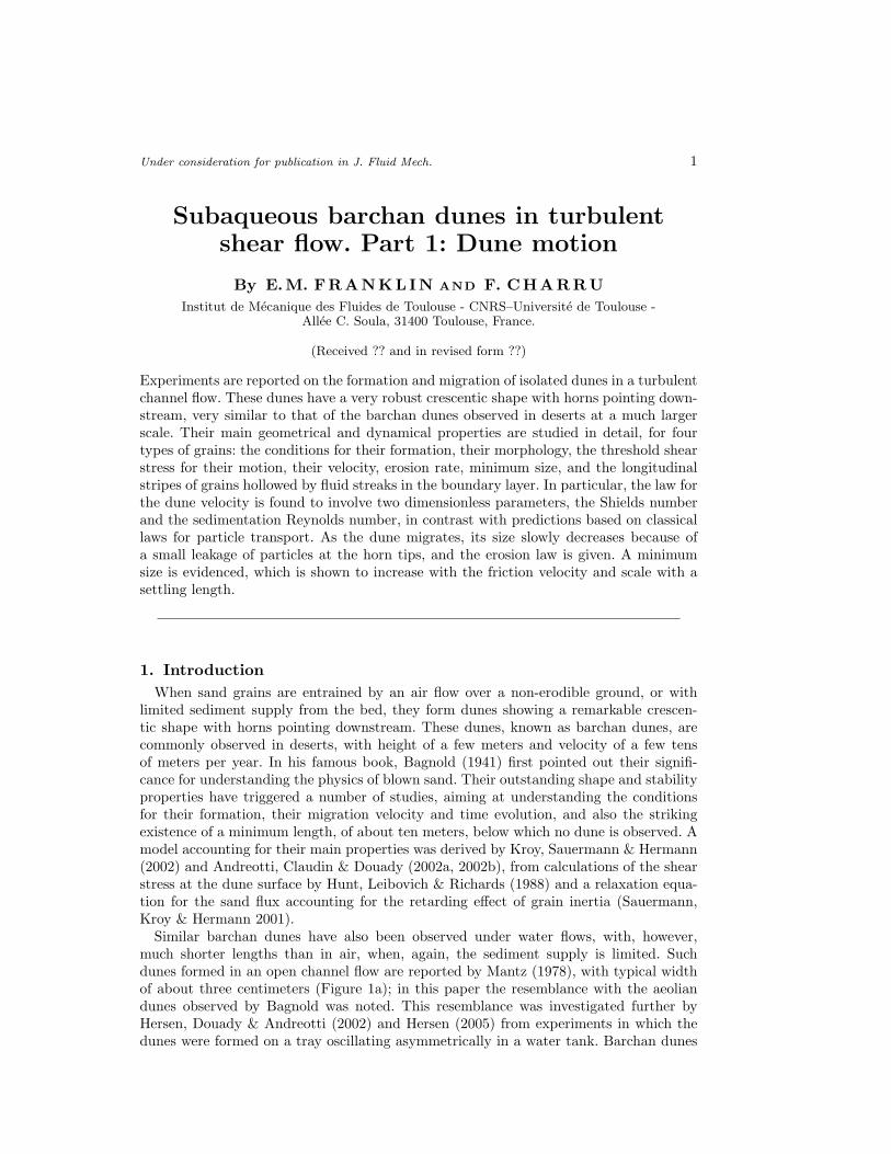
Series d ρp Vfall Refall Rep,max θmax Symbolmm kg m−3 mm s−1

1 0.12 2600 10.7 1.28 3.0 0.34 �2 0.18 2600 20.6 3.71 4.5 0.23 ◦3 0.51 2600 78.4 40.0 12.9 0.08 �4 0.19 3760 35.0 6.65 4.8 0.12 ∗

Table 1. Particles properties, settling velocity Vfall and Reynolds number Refall, maximumvalues of the particle Reynolds number Rep and Shields number θ, and corresponding symbolsin the figures.

of these numbers. Note that the particle Reynolds numbers was smaller than 13 for allexperiments, so that small viscous effects on the grain motion are likely to be expected.

3. Dune motion3.1. Dune formation

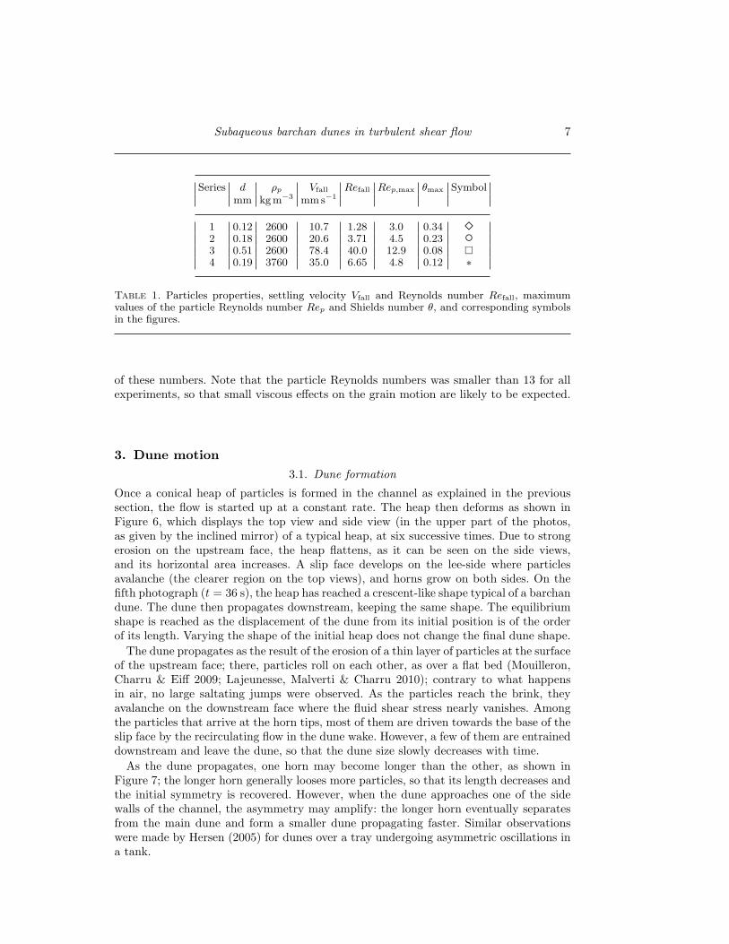
Once a conical heap of particles is formed in the channel as explained in the previoussection, the flow is started up at a constant rate. The heap then deforms as shown inFigure 6, which displays the top view and side view (in the upper part of the photos,as given by the inclined mirror) of a typical heap, at six successive times. Due to strongerosion on the upstream face, the heap flattens, as it can be seen on the side views,and its horizontal area increases. A slip face develops on the lee-side where particlesavalanche (the clearer region on the top views), and horns grow on both sides. On thefifth photograph (t = 36 s), the heap has reached a crescent-like shape typical of a barchandune. The dune then propagates downstream, keeping the same shape. The equilibriumshape is reached as the displacement of the dune from its initial position is of the orderof its length. Varying the shape of the initial heap does not change the final dune shape.

The dune propagates as the result of the erosion of a thin layer of particles at the surfaceof the upstream face; there, particles roll on each other, as over a flat bed (Mouilleron,Charru & Eiff 2009; Lajeunesse, Malverti & Charru 2010); contrary to what happensin air, no large saltating jumps were observed. As the particles reach the brink, theyavalanche on the downstream face where the fluid shear stress nearly vanishes. Amongthe particles that arrive at the horn tips, most of them are driven towards the base of theslip face by the recirculating flow in the dune wake. However, a few of them are entraineddownstream and leave the dune, so that the dune size slowly decreases with time.

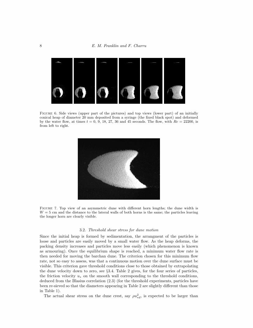
As the dune propagates, one horn may become longer than the other, as shown inFigure 7; the longer horn generally looses more particles, so that its length decreases andthe initial symmetry is recovered. However, when the dune approaches one of the sidewalls of the channel, the asymmetry may amplify: the longer horn eventually separatesfrom the main dune and form a smaller dune propagating faster. Similar observationswere made by Hersen (2005) for dunes over a tray undergoing asymmetric oscillations ina tank.


Figure 6. Side views (upper part of the pictures) and top views (lower part) of an initiallyconical heap of diameter 20 mm deposited from a syringe (the fixed black spot) and deformedby the water flow, at times t = 0, 9, 18, 27, 36 and 45 seconds. The flow, with Re = 22200, isfrom left to right.

Figure 7. Top view of an asymmetric dune with different horn lengths; the dune width isW = 5 cm and the distance to the lateral walls of both horns is the same; the particles leavingthe longer horn are clearly visible.

3.2. Threshold shear stress for dune motion

Since the initial heap is formed by sedimentation, the arrangment of the particles isloose and particles are easily moved by a small water flow. As the heap deforms, thepacking density increases and particles move less easily (which phenomenon is knownas armouring). Once the equilibrium shape is reached, a minimum water flow rate isthen needed for moving the barchan dune. The criterion chosen for this minimum flowrate, not so easy to assess, was that a continuous motion over the dune surface must bevisible. This criterion gave threshold conditions close to those obtained by extrapolatingthe dune velocity down to zero, see §3.4. Table 2 gives, for the four series of particles,the friction velocity u∗ on the smooth wall corresponding to the threshold conditions,deduced from the Blasius correlation (2.3) (for the threshold experiments, particles havebeen re-sieved so that the diameters appearing in Table 2 are slightly different than thosein Table 1).

The actual shear stress on the dune crest, say ρu2∗d, is expected to be larger than


Series d D θt u∗t u∗ u∗t/u∗mm – – mm s−1 mm s−1 –

1 0.11 2.75 0.073 11.2 9.0 1.242 0.21 5.26 0.047 12.4 10.7 1.163 0.53 13.3 0.031 15.9 13.1 1.224 0.21 6.31 0.042 15.4 11.9 1.29

Table 2. For each of the four series, dimensionless number D, corresponding threshold Shieldsnumber θt and threshold friction velocity u∗t, friction velocity at the onset of dune motion u∗as given by (2.3), and ratio u∗t/u∗.

that on the smooth wall, ρu2∗, due to both form and roughness effects. This shear stress

was estimated as follows. The threshold shear stress for particle motion on a flat bedcorresponds a critical Shields number

θt =ρu2∗t

(ρp − ρ)gd. (3.1)

This number is about 0.05, and weakly depends on the particle Reynolds number (or thedimensionless number D3 = (ρp/ρ−1)gd3/ν2 which represents a Reynolds number basedon the Stokes falling velocity). For each series of particles, this number can be calculatedusing the empirical correlation θt(D) proposed by Soulsby & Whitehouse (1997). Thenthe corresponding threshold friction velocity on the dune, u∗t, can be obtained from (3.1).The friction velocity thus determined, as well as the ratio u∗t/u∗, are reported in Table2. It appears that u∗t/u∗ is approximately constant and close to 1.2. In other words, theactual shear stress on a dune is approximately (1.2)2 ≈ 1.4 times larger than that on thesmooth wall, at the threshold conditions. Although this number might depend on thedune height, no significant variation was found, which is consistent with the fact that thisheight, in the range 1–7 mm, was much smaller than the channel height. More generally,for dune widths less than one-half of the channel width and dune heights less than onetenth of the channel height, confinement had negligible effect on the observations reportedin this paper. A detailed analysis of the variation of the shear stress along the dune willbe addressed in the second part of this paper.

3.3. Dune morphologySince Bagnold’s observations, the shape of aeolian barchan dunes, in particular theirapparent scale invariance and the existence of a minimum size, has been extensivelyinvestigated (Sauerman et al. 2000; Andreotti, Claudin & Douady 2002a; Elbelrhiti,Andreotti & Claudin 2008). The length L, width W , height H and horn length Lh, asdefined in Figure 1c, are the parameters generally reported. Measurements exhibit largescatter due to wind variations, but linear relationships emerge after averaging betweenthe characteristic lengths, of the form H = cH(L−L0). Typically, cH ≈ 0.2 and L0 ≈ 10m; however, these coefficients depend on the dune field investigated. It has been notedthat the offset length L0 breaks the proportionality of the height and length, i.e. aeoliandunes are not scale invariant. The significance of this offset length has been related tothe observation that all aeolian dunes are larger than a minimum size; this point will bediscussed further in Section 3.6. Another point of the discussion is the position of the


!30 !20 !10 0 100

1

2

3

4

5

x (mm)

y (m

m)

Figure 8. Typical profile of a dune. Thick line: measured profile; (− · −), fit (3.2) withL = 38 mm, hM = 3.6 mm, and xM = 4 mm; (− −), fit from (3.3) with L = 45 mm andthe same hM and xM ; (—) parabolic fit with L = 42 mm, and the same hM and xM .

dune top, which may coincide with the brink of the slip face for small dunes, or, for largerones, correspond to the crest of a smooth dome located upstream of the brink.

As mentioned in the introduction, barchan dunes under water have already been re-ported, but with a centimetric size, much smaller than that of aeolian dunes. (The largedunes observed at the bottom of shallow seas or rivers, of a few meters high, are rathertwo-dimensional structures which have grown on erodible beds (ASCE 2002).) However,the question of their morphology and scale invariance has not been investigated yet.

The first point to address is the longitudinal profile h(x) in the vertical symmetry planeof the dune, which is closely related to the particle flux as it will be shown in Section 3.4.Figure 8 displays the profile of a typical dune. The left side corresponds to the upstreamface, with slope of the order of 7◦, whereas the steeper right side corresponds to thehorn; the avalanche face, hidden by the horn, has a slope close to 30◦. The origin x = 0corresponds to the highest point of the profile, which coincides with the position of thebrink in the symmetry plane of the dune. The profile of a dune or hill often consideredin theoretical analyses is the symmetrical bell shape (Benjamin 1959, Hunt, Leibovich &Richards 1988)

h(x) =hM

1 + (x− xM )2/L2. (3.2)

Fitting the measured profile with this bell shape (the dotted-dashed line in the figure)shows that (i), eq. (3.2) represents nicely the upstream face near the brink (−20 <x (mm) < 0) but decreases too slowly near the foot (−40 < x (mm) < −20), and (ii),the top of the bell does not coincide with the brink, it is located downstream at adistance xM = 4 mm ≈ hM . The parabolic shape suggested by Sauermann et al. (2000),h(x) = hM (1− (x− xM )2/L2), provides better agreement (plain line). The best fit overthe whole profile was however provided by the cosine shape

h(x) = hM cosπ(x− xM )

2L, (3.3)

with the same xM and hM (dashed line). The length L = 45 mm for the cosine shape isslightly larger than for the bell and parabolic shapes, and close to the length L = 48 mmdefined in Figure 1c from the top view. The feature that the slope of the profile is positive


0 20 40 60 800

20

40

60

80

100

L (mm)

W (m

m)

0 20 40 60 800

20

40

60

80

100

L (mm)

W (m

m)

0 20 40 60 800

20

40

60

80

100

L (mm)

W (m

m)

0 20 40 60 800

20

40

60

80

100

L (mm)

W (m

m)

(a) (b)

(c) (d)

Figure 9. Width W versus length L for all dunes, for Reynolds number Re = 13900 (∗),Re = 16200 (4), Re = 17400 (+), Re = 18500 (�), Re = 19700 (×), Re = 20800 (◦), Re = 23100(�). (a), series 1; (b), series 2; (c), series 3; (d), series 4; the straight line corresponds to eq.(3.4).

at the brink (i.e. that the summit of the fitting curve is located downstream of the brink,at a distance of the order of the dune height) was quite general in the explored range offluid flow rates.

The characteristic lengths defined in Figure 1c have been measured for a large numberof dunes, more than six hundreds, as they had reached their equilibrium shape, i.e. afterthey had travelled a distance larger than twice the size of the initial heap. Figure 9adisplays the width W versus the length L for Series 1, for seven flow Reynolds numbers.It appears the data points gather close to the straight line

W = cW L, with cW = 1.1, (3.4)

with no significant dependence on the flow Reynolds number Re. The scatter, althoughnot negligible, is however much smaller than that for desert dunes, because of the constantdirection and velocity of the water flow. Comparison of Figures 9a-c (glass particles of thesame density) shows that increasing the grain diameter by a factor 5 has no significanteffect on the relationship between L and W . Comparing Figures 9b and 9d (particleswith the same diameter and density increased by a factor 1.5), no significant change canagain be noted. Finally, the linear relationship between the width and length appears tobe independent of the particle diameter and density, as well as of the flow velocity, and(3.4) provides a good fit for all the measurements.

Dune heights were measured with the help of the video camera and the inclined mirror.These heights exhibited large scatter for both physical reasons (loose selection mechanism


0 20 40 60 800

2

4

6

8

L (mm)

H (m

m)

0 20 40 60 800

2

4

6

8

L (mm)

H (m

m)

0 20 40 60 800

2

4

6

8

L (mm)

H (m

m)

0 20 40 60 800

2

4

6

8

L (mm)

H (m

m)

(a) (b)

(c) (d)

Figure 10. Height H versus length L, for same Reynolds numbers as in Figure 9 (same symbols).(a), series 1; (b), series 2; (c), series 3; (d), series 4; solid line: (3.5) with L0 = 70 d; dashed line(3.5) with L0 = 12 mm.

of the height for given horizontal size) and technical reasons (uncertainties related to theuse of the mirror system). However, it appeared that the scatter could be reduced byremoving the most asymmetric dunes, i.e. dunes with horns of quite different lengths asthat shown in Figure 7. Figure 10 displays the height of dunes whose horn lenghts differby less than 20% of their mean value (this corresponds to the removal of 60% of themeasurements). For Series 1 (Figure 10a), most data points gather close to the solid linedefined as

H = cH(L− L0) (3.5)

with cH = 0.12 and L0 = 70 d. However, a few dunes have height smaller by a factor 2.Figures 10b and 10d show that doubling the grain diameter or density, the relationship(3.5) still holds; however, a constant offset length L0 = 12 mm (dashed line) also providesa good fit of the data from the three series 1, 2 and 4. The dune heights from series 3(large glass grains, Figure 10c) exhibit more complicated features: large dunes (L & 50mm) are still accounted for by the relation (3.5) with L0 = 70 d, but small dunes arecloser to the line with L0 = 12 mm; the departure from (3.5) may be due to the smallratio H/d of these dunes.

Horns are the most distinctive feature of barchan dunes and play an essential rolein their stability (Hersen 2004), so that horn lengths may be considered as their mostrelevant geometrical property. Figure 11 displays the horn length Lh versus the lengthL, for the same symmetric dunes as in Figure 10. Figure 11a for Series 1 shows that the


0 20 40 60 800

5

10

15

20

L (mm)

Lh (m

m)

0 20 40 60 800

5

10

15

20

L (mm)

Lh (m

m)

0 20 40 60 800

5

10

15

20

L (mm)

Lh (m

m)

0 20 40 60 800

5

10

15

20

L (mm)

Lh (m

m)

(a) (b)

(c) (d)

Figure 11. Horn length Lh versus length L, for same Reynolds numbers as in Figure 9 (samesymbols). (a), series 1; (b), series 2; (c), series 3; (d), series 4; solid line: (3.6) with L0h = 30 d;dashed line (3.6) with L0h = 6 mm.

horn length Lh increases linearly with the length L, according to the relationship

Lh = ch(L− L0h), (3.6)

with ch = 0.3 and L0h = 30 d. Again, no dependence on the flow Reynolds numberis visible. Doubling the grain diameter (Figure 11b for series 2) or the relative density(Figure 11d for series 4) does not change the relationship (3.6); however, a constant offsetlength L0h = 6 mm would also provide a good fit (see the dashed lines), as for the duneheights. The dunes from series 3 shown in Figure 11c have shorter horns, still distributedclose to (3.6) although the scatter is large; this scatter is likely to be related, again, tosmall heights (H/d < 10). From (3.5) and (3.6), the heights and horn lengths appear tobe nearly proportional, as noted by Andreotti et al. (2002a) for aeolian dunes.

Finally, the relationships between the dimensions of barchan dunes in water appearto be linear, similarly to those for aeolian dunes. No significant change appears in theslope coefficients cW , cH and ch, by varying the diameter by a factor 2 (between Series1 and 2), or the density by a factor 1.5 (between Series 2 and 4), or the flow velocity bya factor 1.7 (for all Series). The offset lengths L0 and L0h do not depend on the particledensity and the flow velocity; they might depend on the particle diameter but a specificinvestigation of small dunes would however be needed for a definite conclusion to bedrawn.

The above linear relations between the dune dimensions are similar to those foundby previous investigations, with similar slope coefficients cW , cH and ch. In particular,Hersen et al. (2002) and Hersen (2005) found cH = 0.11 for subaqueous dunes (we


find 0.12); for aeolian dunes, Sauermann et al. (2000) found cH = 0.16 in SouthernMorocco and the compilation by Andreotti et al. (2002a) gives cH = 0.18. The offsetlength L0 and L0h, which break the self-similarity of small dunes, are however quitedifferent: whereas they are of a tens of meters for aeolian dunes, they are much smaller,of about ten millimeters, for subaqueous dunes. As noted by Hersen et al. (2002), using`drag = (ρp/ρ)d as the length scale for the dune dimensions, the data for subaqueaousand aeolian dunes nearly gather. This point will be discussed further in §3.6.

3.4. Dune velocityLet’s first consider the classical theory for the velocity Vd of a two-dimensional aeoliandune (invariant in the transverse direction) with brink normal to the air flow, withoutany sand flux from upstream (Bagnold 1941). As long as the volumetric grain flux perunit width at the brink, qH , is deposited on the avalanche face, mass conservation givesthe velocity

Vd =qHH, (3.7)

where H is the height of the brink. This equation can also be derived from the local massconservation equation ∂th+ ∂xq = 0 with the shape-invariance condition ∂th = −Vd∂xh.Integrating this equation along the windward face gives

qH − q(x) = Vd(H − h(x)),

which relates the local particle flux q(x) to the local dune height h(x). From this equation,(3.7) is recovered when the incoming flux from upstream is zero (q = 0 at the foot of thedune where h = 0). Assuming that the particle flux qH is in equilibrium with the localshear stress τH at the brink, which is approximately 1.8 times the shear stress ρairu

2∗

over the surrounding flat ground (Andreotti et al. 2002a), a semi-empirical transport lawof the form qH ∝ (ρair/ρp)u3

∗/g can then be used. From these considerations, the dunevelocity is given by

Vd

u∗∝ ρair

ρp

u2∗

gH.

This crude model gives the right order of magnitude of a few tens of meters per year.However, the available observations clearly show that the scaling Vd ∝ 1/H overestimatesthe velocity of small dunes. Improvements have been proposed, accounting for a betterdescription of the hydrodynamics over the dune and the retarding effect of particle inertiaon the particle flux (Andreotti et al. 2002b; Kroy et al. 2002; Hersen 2004). In particular,relationships of the form Vd ∝ 1/(H +H0), where H0 is an offset height of a few meters,or Vd ∝ 1/L, were shown to provide better predictions. Thorough assessment of thesetheories however comes up against the difficulty of observations on large space and timescales, and also the large scatter due to the variable flow conditions and sand supply inthe open atmosphere.

Under water, a straightforward translation of the theory sketched above consists inreplacing the transport law qH ∝ (ρair/ρp)u3

∗/g by one for water, e.g. the widely usedMeyer-Peter & Muller law (Wong & Parker 2006),

qHVrefd

= 4.0 (θH − θt)3/2, (3.8)

where θH is the Shields number (2.5) with the shear stress evaluated at the brink, andVref = ((ρp/ρ − 1)gd)1/2. (Note that in the limit of small fluid density and large shearstress, (3.8) reduces to the relationship for air.) To our knowledge, the only observationsof the velocity of subaqueous dunes are those of Hersen (2005) for dunes on a tray


0 0.02 0.040

1

2

3

x18

1/L (mm!1)

Vd (m

m/s)

0 0.02 0.040

1

2

3

4

5

x35

1/L (mm!1)

Vd (m

m/s)

0 0.02 0.040

2

4

6

8 x130

1/L (mm!1)

Vd (m

m/s

)

0 0.02 0.040

0.2

0.4

0.6

0.8

1

1/L (mm!1)

Vd (m

m/s

)

(a) (b)

(c) (d)

Figure 12. Dune velocity Vd versus the inverse length 1/L for series 1 (a), series 2 (b), series3 (c) and series 4 (d). Symbols correspond to given Reynolds number, see caption of Figure 9(for the lowest one (∗), the small velocity is multiplied by the factor shown on the right of theline). Straight lines emphasize the linear dependence Vd ∝ 1/L for given flow conditions.

undergoing asymmetric oscillations, and of Taniguchi & Endo (2007) for dunes underalternating flows. Thus, no velocity measurement under steady conditions is available, sothat the prediction (3.7-3.8) has not been assessed yet.

In the present experiments, dune velocities have been investigated by varying both thegrain properties and the fluid velocity. Velocities have been determined from the distancetravelled by the foot of the slip face, divided by the corresponding time; the distance wasof a few dune lengths (typically between 10 or 20 centimeters), and times ranged from20 seconds to 40 minutes.

Figure 12 displays the velocity Vd as a function of the inverse dune length L−1, forseveral flow Reynolds number, and for the four series (for clarity, the small values of Vd

for the smallest Reynolds number (∗) have been multiplied by the coefficient shown on theright of the line). For the small glass particles of series 1, Figure 12a shows that, for givenReynolds number, the velocity scales with the inverse length, Vd ∝ L−1, as predicted bythe mass conservation argument (3.7) along with the scale invariance L ∝ H. Figures12b-c-d display the dune velocity for the series 2, 3 and 4, showing the same features.For the smallest Reynolds number, linear regression suggested that the velocity ratherfollows Vd ∝ (L + L0)−1, with a length L0 of a few millimeters, but the scatter of themeasurements prevented any precise determination.

The increase of the dune velocity with Reynolds number, for given dune length, is alsoclearly visible in Figure 12. This dependence has been studied further by consideringthe velocity Vd,60 of dunes of the same length, L = 60 mm, obtained from the linear


10 15 20 250

2

4

6

u* (mm/s)

Vd (m

m/s)

0.01 0.1

0.1

1

10

! ! !t

V d/Vre

f L/d

(a) (b)

Figure 13. Velocity of dunes with the same length L = 60 mm, for all series (see Table 1 forsymbols); (a), dimensional velocity versus the wall friction velocity u∗; (b), normalized velocityVd/Vref(L/d) versus θ − θt in log-log scales; straight line: eq. (3.7).

regression lines; such dunes all have nearly the same height, about 5–6 mm accordingto (3.5). As shown in Figure 13a for all series, the velocity Vd,60 increases strongly withthe friction velocity u∗; for given u∗, it increases with the particle diameter (compareseries 1, 2 and 3 for the glass particles), and decreases with the particle density (compareseries 2 and 4 for the glass and zirconium particles of nearly same diameter d ≈ 0.2 mm).For each of the four series, extrapolating the velocity down to zero provides an estimateof the threshold friction velocity below which the dune no longer moves. This thresholdis in good agreement with that found independently from the visual observation of thestopping of particle motion at the dune surface, and reported in Table 2.

In order to assess Bagnold’s theory, Figure 13b displays the dune velocity, normalizedwith Vrefd/L, as a function of θ − θt, in logarithmic scales. Shields numbers have beencalculated with the friction velocity u∗d = 1.2u∗, i.e. by assuming that the ratio 1.2found at threshold still holds above threshold. It appears that for all the four series, thedune velocity follows power laws of the form Vd/Vref ∝ (d/L)(θ − θt)n, with the sameexponent n ≈ 2.5 but different numerical coefficients. Figure 13b also displays the linecorresponding to Bagnold’s prediction (3.7) with the particle flux at the crest given bythe Meyer-Peter & Muller correlation. It appears clearly that this prediction does notprovide the right velocity:• it does not account for the dependence on the type of particles;• the exponent 3/2 of the power law is too small.

Note that taking a different bedload transport law, from those available in the litterature,do not provide better agreement.

Attempting to gather the data points of the four series on the same master curve, itfirst appeared that dividing the dune velocity by the true falling velocity Vfall or thefriction velocity u∗d, instead of the reference velocity Vref , does not improve significantlythe picture. In fact, Figure 13b strongly suggests that one single dimensionless parameter,i.e. the Shields number, is not sufficient to account for dune velocities. This observationis consistent with the fact that particle Reynolds numbers are not large (see Table 1), sothat some dependence with this number may be expected.

A good collapse of the data points is achieved when the dune velocity is divided


0.01 0.1

10!2

100

102

! ! !t

V d/Vnorm

Figure 14. Normalized dune velocity versus θ − θt in log-log scales, for all series (see Table 1for symbols). Vnorm = VrefResd/L, straight line: eq. (3.9).

by the sedimentation Reynolds number, as shown in Figure 14 where the straight linecorresponds to

Vd

Vref= 280Res

d

L(θ − θt)2.5. (3.9)

From (3.9), the particle flux qH at the dune crest can be deduced from the mass con-servation equation (3.7) and the morphological relation (3.5). Ignoring the small offsetlength L0 in (3.5), qH is found to be

qHVrefd

= 34Res(θ − θt)2.5. (3.10)

This relation is different, as expected, from the usual relationships for turbulent flowwhich typically involve the exponent 3/2 for the dependence with the Shields number,as the Peter-Meyer & Muller relation (3.8). It is also different, although closer, from thequadratic relation qH/Vrefd ∝ θ(θ − θt) found from viscous flow experiments on a flatbed by Charru, Mouilleron & Eiff (2004) (in these experiments, the grain properties werenot varied so that Res was constant). Note that the closeness of (3.10) with viscous flowresults is consistent with the fact that here, the particle Reynolds number was alwayssmaller than 13 (see Table 1), so that the moving grains hardly emerged from the viscoussublayer (this point will be discussed further in the Part 2 of this paper, in relationwith shear stress measurements). Finally, (3.9) appears as as a good fit for grains withdifferent density and diameter, but its physical meaning remains to be understood.

3.5. Erosion rateAs a dune propagates, it slowly looses particles at the horn tips and its size decreases.Understanding this particle leakage is important in the perspective of modelling theevolution of a field of dunes, where the particles leaving one dune feed another onedownstream.

In the present experiments, a few single dunes have been tracked during a sufficientlylong time for their size evolution to be measured until disappearance. Figure 15a displaysthe time evolution of the width of four dunes, for two types of particles (series 3 and 4) and


0 0.5 1 1.5 2x 104

0

20

40

60

80

t (s)

W (m

m)

102103104101

102

t0 ! t (s) W

(mm

)

(a) (b)

Figure 15. Time variation of the dune width: (a), linear scales; (b), log scales. Symbols: (�):series 3, Re = 13900; (◦): series 3, Re = 16200; (�): series 4, Re = 16200; (∗): series 4,Re = 18500; (—): power law (3.11).

three Reynolds numbers. As the dune size has decreased down to about one centimeter,the horns become unstable, randomly disappearing and appearing again with a timescale of a few seconds. After a few oscillations, the horns definitely disappear and theremaining heap is dispersed by the fluctuations of the turbulent flow. The disappearanceocccurs at a critical time t0 after the beginning of the run, which was typically betweenone and five hours (larger dunes had longer life times). From the measurement of thecritical time or its estimation when the tracking was stopped before the disappearanceof the dune, the width was found to follow the power law W ∝ (t0 − t)1/3, as shown bythe log-log plot in Figure 15b.

From the morphology study presented in section 3.3 and on considering that duneshave self-similar parabolic shapes, their volume V is related to their width by

V ≈ 615

cHc2W

W 3 ≈ 0.03W 3.

Thus the exponent 1/3 forW (t) corresponds to linear decrease of the volume, i.e. constantnumber of particles leaving the horns per unit time, or constant erosion rate. (Note thatan erosion rate proportional to the volume of the dune would result in an exponentialdecrease, which is clearly not the case here.) Let te be the erosion time, i.e. the timeneeded for loosing one grain per horn. Then the variation of the volume of the duneduring dt is

dV = −2πd3

6φdtte

where φ ≈ 0.6 is the volume fraction of the particles. From the above relations, the dunewidth decreases with time as

W

d= 3.9

(t0 − tte

)1/3

. (3.11)

From the above relation and the measured time evolution W (t), the erosion time tecan be deduced for each experiment. The four erosion times corresponding to Figure 15


0 5 10 15 200

0.1

0.2

0.3

0.4

u* (mm/s)

t e (s)

102104106101

102

103

(t0 ! t)/te W

/d

(a) (b)

Figure 16. (a) Erosion time from experiments (symbols) and correlation (3.12) (solid line); (b),dimensionless width versus dimensionless time using the correlation (3.12) for te. (�), series 3,Re = 13900; (◦), series 3, Re = 16200; (�), series 4, Re = 16200; (∗), series 4, Re = 18500.

are shown in Figure 16a, where they appear to depend mainly on the shear velocity u∗(they are nearly equal at the same flow Reynolds number Re = 16200 for series 3 and4). Since the particles at the horn tips hardly emerge from the viscous sublayer (smallparticle Reynolds numbers), the expected scale for the erosion time is the viscous timebased on the wall scales u∗ and ν. It appeared that the following law fits reasonably wellthe measured erosion times:

te = 2ν

(u∗ − u∗e)2 , u∗e = 11 mm s−1 (3.12)

where u∗e is a threshold friction velocity for dune erosion (the erosion time must divergeat threshold). This threshold appears to be slightly lower than the threshold u∗t for dunemotion, which can be understood by the fact that particles are easier to move on thesmooth wall at the tip of the horns than on the rough dune surface. Figure 16b showsthat with the above modelling for the erosion time, all the data points collapse reasonablywell on the same curve for the four dunes.

3.6. Minimum size

As noted by Bagnold (1941, §14.3), aeolian barchan dunes have a minimum height ofabout Hmin ≈ 1 m, and a corresponding minimum length Lmin ≈ 10 m, below whichno dune is observed. The minimum height was interpreted by Bagnold by consideringthe trajectories of the sand grains after they have passed over the brink and enter aregion of stagnant air: below some critical dune height, the grains fall beyond the foot ofthe slip face and are dispersed by the wind. From another point of view, the minimumlength can be interpreted as the distance needed for the particle flux to increase fromzero, at the upwind foot of the dune, up to some saturated value depending on the localshear stress only (Bagnold 1941, §12.9). The length scale associated with the relaxationof the particle flux may be related to several physical phenomena. Sauermann, Kroy &


Figure 17. Successive pictures of the oscillations of the horns and disappearance of a barchandune. Between the first and last pictures, the elapsed time is 20 seconds and the dune hastravelled a distance of four times its initial size, of 15 mm.

Hermann (2001) proposed that it should scale with the saltation length

`salt ≈ 15u2∗g

(3.13)

of the grains expelled from the bed by the impact of the oncoming grains, with a prefactoraccounting for the slowing down of the wind by the saltating cloud. Andreotti et al.(2002b) consider that grain inertia is the dominant mechanism involved in the saturation,so that the relevant length should be an acceleration length of the particles acceleratedfrom rest by the wind. From dimensional analysis, this acceleration length must scalewith the drag length

`drag =ρpρd (3.14)

(which is typically 0.5 meter), and weakly depends on the wind strength (Andreotti etal. 2010). These ideas have also been applied to observations on Mars by Claudin &Andreotti (2006).

Under water, whose density is one thousand times larger than that of air, hydro-dynamic interactions are more complex, and particles roll on each other rather thanexperience large saltating jumps (Lajeunesse et al. 2010). A characteristic length mayhowever dominate: the deposition length

`fall =u∗Vfall

d, (3.15)

which represents the distance travelled by a grain with velocity u∗ during the fallingtime d/Vfall. This length was introduced by Charru and Hinch (2006) from an erosion-deposition model, and its importance in the selection of the wavelength of ripples wasdiscussed by Charru (2006). In water, the lengths `drag and `fall are of the order of onemillimeter, but they scale differently with the parameters. The measurements reportedin this section are intended to discuss the existence of a minimum size of subaqueousbarchan dunes, and to assess the relevance of `drag or `fall as the scaling length for thisminimum size.

Turning back to our experiments, the size of a dune was found to decrease slowly inthe course of its motion, because of the small leakage of particles at the tip of the hornsas discussed in the previous section. As the size is reduced to the order of one centimeter,the horns become unstable, disappearing and reappearing randomly, as shown by thesequence of six successive photographs displayed in Figure 17. The leakage of particlesincreases strongly, and after a few oscillations of the horns (a few seconds) the dunedisappears.

The time of the disappearance, and the corresponding dune size, were not easy todefine precisely, but the onset of the horn instability was found to be reproducible. The


10 15 20 250

5

10

15

20

25

30

u* (mm/s)

Wm

in (m

m)

0 0.1 0.2 0.3 0.40

50

100

150

u*/Vref

Wm

in/d

(a) (b)

Figure 18. (a) Minimum width of barchan dunes as a function of the shear velocity, for dunesfrom series 2 (◦), 3 (�) and 4 (∗). (b) Same data presented with d and Vref as the unit lengthand unit velocity.

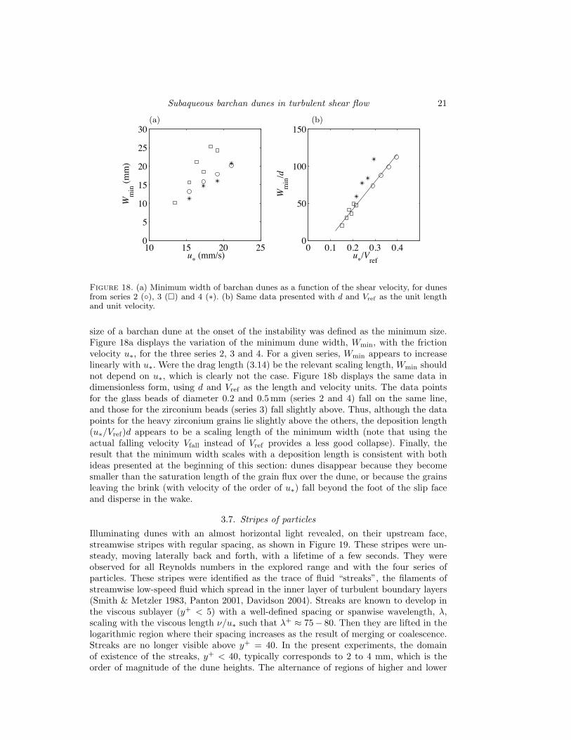
size of a barchan dune at the onset of the instability was defined as the minimum size.Figure 18a displays the variation of the minimum dune width, Wmin, with the frictionvelocity u∗, for the three series 2, 3 and 4. For a given series, Wmin appears to increaselinearly with u∗. Were the drag length (3.14) be the relevant scaling length, Wmin shouldnot depend on u∗, which is clearly not the case. Figure 18b displays the same data indimensionless form, using d and Vref as the length and velocity units. The data pointsfor the glass beads of diameter 0.2 and 0.5 mm (series 2 and 4) fall on the same line,and those for the zirconium beads (series 3) fall slightly above. Thus, although the datapoints for the heavy zirconium grains lie slightly above the others, the deposition length(u∗/Vref)d appears to be a scaling length of the minimum width (note that using theactual falling velocity Vfall instead of Vref provides a less good collapse). Finally, theresult that the minimum width scales with a deposition length is consistent with bothideas presented at the beginning of this section: dunes disappear because they becomesmaller than the saturation length of the grain flux over the dune, or because the grainsleaving the brink (with velocity of the order of u∗) fall beyond the foot of the slip faceand disperse in the wake.

3.7. Stripes of particlesIlluminating dunes with an almost horizontal light revealed, on their upstream face,streamwise stripes with regular spacing, as shown in Figure 19. These stripes were un-steady, moving laterally back and forth, with a lifetime of a few seconds. They wereobserved for all Reynolds numbers in the explored range and with the four series ofparticles. These stripes were identified as the trace of fluid “streaks”, the filaments ofstreamwise low-speed fluid which spread in the inner layer of turbulent boundary layers(Smith & Metzler 1983, Panton 2001, Davidson 2004). Streaks are known to develop inthe viscous sublayer (y+ < 5) with a well-defined spacing or spanwise wavelength, λ,scaling with the viscous length ν/u∗ such that λ+ ≈ 75− 80. Then they are lifted in thelogarithmic region where their spacing increases as the result of merging or coalescence.Streaks are no longer visible above y+ = 40. In the present experiments, the domainof existence of the streaks, y+ < 40, typically corresponds to 2 to 4 mm, which is theorder of magnitude of the dune heights. The alternance of regions of higher and lower


Figure 19. Top view of a dune illuminated with an almost horizontal light, showingstreamwise stripes (the flow is from left to right, particles from series 4).

0 100 200 3000

10

20

30

n

0 100 200 3000

10

20

30

0 100 200 3000

10

20

30

!+

n

0 100 200 3000

10

20

30

40

!+

(a) (b)

(c) (d)

Figure 20. Histograms of the dimensionless spanwise spacing of the stripes λ+ = λu∗/ν, for(a) series 1, (b) series 2, (c) series 3, (d) series 4.

velocity is associated with pairs of counter-rotating streamwise vortices, which promotehigher erosion of particles along the lines where the streamwise velocity is higher and thespanwise velocity diverges, and higher deposition in between these lines, explaining theobserved relief.

The spacing λ of particle stripes was measured for flow Reynolds numbers in the range18000–28000, for the four series of particles. Figure 20 displays the distribution of these


wavelengths, in wall units. It appears that for the particles of series 1, 2 and 4 (Figures20a, 20b and 20d), with diameter in the range 0.1–0.2 mm corresponding to d+ = 1.7–4.5, the distribution has a well-defined peak at λ+ ≈ 100, and a long tail on the sideof large wavelengths. For the larger particles of series 3 (d = 0.5 mm, d+ = 9.7–13.3,Figure 20c), which protude out of the viscous sublayer, the distribution, although notconverged, indicates a larger spacing of about λ+ ≈ 150. These values correspond tothose of streaks on smooth walls (Smith & Metzler 1983), and confirm that the observedstripes of particles are traces of fluid streaks.

Another mechanism could be invoked for the existence of stripes, related to the cur-vature of the streamlines over a dune: the centrifugal Gortler instability of a boundarylayer flow over a concave wall. For a turbulent boundary layer, this instability gives rise tounsteady streamwise vortices, and has been recognized to be responsible of sand stripesin the scour-hole problem of a wall-jet flowing over a bed of particles (Hopfinger et al.2004). However, as shown below, this instability is not relevant here. For the appear-ance of Gortler vortices, the curvature R−1 must be high enough; the condition usuallyconsidered, δ/R ≥ 0.01 (Floryan 1991), with R = H/L2, is fulfilled here. However, theinstability is weak and the growth of the vortices noticeably slow; following Hopfinger etal. (2004), the spatial growth rate is (Reδm

δm)−1, where δm is the momentum thicknessand Reδm

is a Reynolds number based on δm and an eddy viscosity such that Reδm≈ 30.

With δm ≈ δ/10, the typical distance from the upstream foot of a dune at which theinstability might be observed would be 3δ = 90 mm, which is larger than all the observeddune lengths. Moreover, the centrifugal instability amplifies the largest eddies present inthe boundary layer, leading to vortices with spanwise wavelength usually about twicethe boundary layer thickness (Floryan 1991). Such a wavelength, here of 60 mm, is muchlarger than the observed ones. Therefore, the Gortler instability cannot be invoked forexplaining the observed stripes. Finally, it can be noted that streaks may represent animportant mobilizing force in the erosion process, corresponding to an effective shearstress, active in the sediment transport, larger than the actual shear stress.

4. Summary and conclusionWhen a liquid flow transports a small amount of heavy particles, the particles gather to

form dunes with crescentic shape, with size of a few centimeters. Their main features are agentle slope on the upstream face, a sharp brink above a slip face downstream, and hornspointing downstream. These dunes, similar to the barchan dunes observed in deserts, arevery robust structures. Their turnover time, i.e. the time needed for a dune to travela distance equal to its length, is of the order of one minute, which makes subaqueousdunes much easier to study than the much larger and slower aeolian dunes (for which theturnover time is of the order of one year). The geometrical and dynamical properties ofseveral hundreds of these dunes were investigated for flow Reynolds number up to 21000,for four types of grains of different diameter and density. The main observations can besummarized as follows.• A heap of particles deposited in the channel quickly evolves to a barchan dune,

within a time of the order of their turnover time.• The width, height and horns length are linear functions of the dune length, with an

offset of a few millimeters which breaks the self-similarity of small dunes. These relationsappear to be independent of the fluid velocity and the grain density and diameter. Theoffset length may however depend weakly on the particle diameter, but the scatter of themeasurements prevented any definite conclusion to be drawn about this point. The slope


of the upstream dune profile does not vanish at the brink: the summit of the envelope ofthe profile is situated at a distance of about one dune height downstream.• For small flow rates, the particles are at rest and the dune does not move. From the

Shields curve and visual observation of the onset of particle motion, it was found thatthe shear stress on the dune, ρu2

∗d, is larger by a factor 1.4 than that on the smooth wallof the channel.• The velocity of dunes was found to be inversely proportional to their size, as pre-

dicted by a mass conservation argument. An empirical relationship for the dimensionlessvelocity was derived, on which all the data points collapse well. This relationship involvesnot only on the dimensionless shear stress (the Shields number θ) but also sedimentationReynolds number (or the particle Reynolds number). This suggests that viscous effectsare not negligible with regard to the particle transport, which is consistent with the factthe particle diameter, in wall units ν/u∗d, was smaller than 13.• As a dune migrates, it looses a few particles at the tip of its horns, so that its size

slowly decreases. The width was found to decrease according to the power law (W/d)3 ∝(t0 − t)/te where t0 corresponds to the dune disappearance and te is an erosion time. Aconsequence of this law is that erosion does not depend on the dune size and is governedby the hydrodynamics in the vicinity of the horn tip. Modelling the erosion time with aviscous scale, all the traces of W (t) collapse on the same curve.• Barchan dunes exhibit a minimum size below which the horns become unstable and

oscillate and the dune quickly disappears. The minimum width increases linearly withthe friction velocity and scales roughly with the deposition length

√θ d. This result is

consistent with two different explanations: dunes disappear because they become smallerthan the saturation length of the grain flux over the dune, or because the grains leavingthe brink fall beyond the foot of the slip face and disperse in the wake.• Longitudinal stripes of particles were observed on the upstream face of the dunes.

These stripes have a spanwise spacing λ+ ≈ 150, in wall units, and are formed by thewell-known longitudinal streaks which develop in the viscous sublayer of a turbulentboundary layer. These streaks are likely to enhance particle transport.

Finally, subaqueous barchan dunes appear as very robust structures which may migrateover long distances. At moderate flow rates, they are the main mode of particle transport.Their outstanding stability properties —which are likely to involve the small spanwiseparticle flux, particle relaxation effects, and the flow structure in the dune wake— remainto be understood. Beyond the study of isolated dunes, two situations would also be ofinterest: (i) as the particle flux is increased, dunes with different size and different velocityinteract, and may form a continuous rippled bed; (ii) as the fluid flow rate is increased,particles escape the dune brink and suspension occurs. These questions are left for futureinvestigation.

We are grateful to the French Agence Nationale de la Recherche for partial finan-cial support of this study (#ANR-07-BLAN-0180-01), and to the Brazilian governmentfoundation CAPES for the scholarship grant of E. M. Franklin.

REFERENCES

Al-lababidi, S., Yan, W., Yeung, H., Sugarman, P. & Fairhurst, C. P. 2008 Sand trans-port characteristics in water and two-phase air/water flows in pipelines. Proc. of the 6thNorth American Conference on Multiphase Technology , 159–174.

Andreotti, B., Claudin, P. & Douady, S. 2002a Selection of dune shapes and velocities.Part 1: dynamics of sand, wind and barchans. Eur. Phys. J. B 28, 321–339.


Andreotti, B., Claudin, P. & Douady, S. 2002b Selection of dune shapes and velocities.Part 2: a two-dimensional modelling. Eur. Phys. J. B 28, 341–352.

Andreotti, B., Claudin, P. & Pouliquen, O. 2010 Measurements of the aeolian sand trans-port saturation length. Geomorphology 123, 343–348.

ASCE task committee on flow and transport over dunes 2002 Flow and transport overdunes. J. Hydr. Engrg. 128, 726–728.

Bagnold, R. A. 1941 The physics of blown sand and desert dunes. Chapman & Hall, London.

Charru, F. 2006 Selection of the ripple length on a granular bed sheared by a liquid flow. Phys.Fluids 18, 121508.

Charru, F., Mouilleron, H. & Eiff, O. 2004 Erosion and deposition of particles on a bedsheared by a viscous flow. J. Fluid Mech. 519, 55–80.

Claudin, P. & Andreotti, B. 2006 A scaling law for aeolian dunes on Mars, Venus, Earth,and for subaqueous ripples. Earth Planetary Sci. Lett. 252, 30–44.

Clift, R., Grace, J. R. & Weber, M. E. 1978 Bubbles, drops and particles. Academic Press.

Davidson, P. A. 2004 Turbulence: An Introduction for Scientists and Engineers. Oxford Uni-versity Press.

Elbelrhiti, H., Andreotti, B. & Claudin, P. 2008 Barchan dune corridors: field character-ization and investigation of control parameters. J. Geophys. Res. 113, F02S15.

Floryan, J. M. 1991 On the Gortler instability of boundary layers. Prog. Aerospace Sci. 28,235–271.

Hersen, P. 2004 On the crescentic shape of barchan dunes. Eur. Phys. J. B 37, 507—514.

Hersen, P. 2005 Flow effects on the morphology and dynamics of aeolian and subaqueousbarchan dunes. J. Geophys. Res. 110, F04S07.

Hersen, P., Douady, S. & Andreotti, B. 2002 Relevant lengthscale of barchan dunes. Phys.Rev. Lett. 89, 264301.

Hopfinger, E. J., Kurniawan, A., Graf, W. H. & Lemmin, U. 2004 Sediment erosion byGortler vortices: the scour-hole problem. J. Fluid Mech. 520, 327–342.

Hunt, J. C. R., Leibovich, S. & Richards, K. J. 1988 Turbulent shear flows over low hills.Q. J. R. Meteorol. Soc. 114, 1435–1470.

Kroy, K., Sauermann, G. & Herrmann, H. J. 2002 Minimal model for aeolian sand dunes.Phys. Rev. E 66, 031302.

Lajeunesse, E., Malverti, L. & Charru, F. 2010 Bedload transport in turbulent flow at thegrain scale: experiments and modeling. J. Geophys. Res. 115, F04001.

Mantz, P. A. 1978 Bedforms produced by fine, cohesionless, granular and flakey sedimentsunder subcritical water flows. Sedimentology 25, 83–103.

Melling, A. & Whitelaw, J. H. 1976 Turbulent flow in a rectangular duct. J. Fluid Mech.78, 289–315.

Mouilleron, H., Charru, F. & Eiff, O. 2009 Inside the moving layer of a sheared granularbed. J. Fluid Mech. 628, 229–239.

Nagib, H. M. & Chauhan, K. A. 2008 Variations of von Karman coefficient in canonical flows.Phys. Fluids 20, 101518.

Panton, R. L. 2001 Overview of the self-sustaining mechanisms of wall turbulence. Prog.Aerospace Sci. 37, 341–383.

Sauermann, G., Rognon, P., Poliakov, A. & Herrmann, H. J. 2000 The shape of thebarchan dunes of Southern Morocco. Geomorphology 36, 47–62.

Sauermann, G., Kroy, K. & Herrmann, H. J. 2001 Continuum saltation model for sanddunes. Phys. Rev. E 64, 031305.

Schlichting, H. 1979 Boundary-Layer Theory. McGraw-Hill.

Smith, C. R. & Metzler, S. P. 1983 The characteristics of low-speed streaks in the near-wallregion of a turbulent boundary layer. J. Fluid Mech. 129, 27–54.

Soulsby, R. L. & Whitehouse, R. J. S. 1997 Threshold of sediment motion in coastal envi-ronments. Proc. Australasian Coastal Engng and Ports Conf., 149–154.

Taniguchi, K. & Endo, N. 2007 Deformed barchans under alternating flows: Flume experi-ments and comparison with barchan dunes within Proctor Crater, Mars. Geomorphology90, 91–100.


Wong, M. & Parker, G. 2006 Reanalysis and Correction of Bed-Load Relation of Meyer-Peterand Mller Using Their Own Database. J. Hydr. Engrg., 132, 1159–1168.

Documents

Subaqueous barchan dunes in turbulent shear ow. Part 1 ...franklin/images/franklin_charru(2011).pdf · Subaqueous barchan dunes in turbulent shear ... By E.M. FRANKLIN AND F. CHARRU