Sub-Daily Multi-Objective Models for Optimizing Hydropower

University of Massachusetts AmherstScholarWorks@UMass AmherstEnvironmental & Water Resources EngineeringMasters Projects Civil and Environmental Engineering

9-2011

Sub-Daily Multi-Objective Models for OptimizingHydropower in the Deerfield RiverKelcy Adamec

Follow this and additional works at: https://scholarworks.umass.edu/cee_ewre

Part of the Environmental Engineering Commons

This Article is brought to you for free and open access by the Civil and Environmental Engineering at ScholarWorks@UMass Amherst. It has beenaccepted for inclusion in Environmental & Water Resources Engineering Masters Projects by an authorized administrator of ScholarWorks@UMassAmherst. For more information, please contact [email protected].

Adamec, Kelcy, "Sub-Daily Multi-Objective Models for Optimizing Hydropower in the Deerfield River" (2011). Environmental &Water Resources Engineering Masters Projects. 44.https://doi.org/10.7275/9DD1-VT19

https://scholarworks.umass.edu?utm_source=scholarworks.umass.edu%2Fcee_ewre%2F44&utm_medium=PDF&utm_campaign=PDFCoverPages

https://scholarworks.umass.edu/cee_ewre?utm_source=scholarworks.umass.edu%2Fcee_ewre%2F44&utm_medium=PDF&utm_campaign=PDFCoverPages


https://scholarworks.umass.edu/cee?utm_source=scholarworks.umass.edu%2Fcee_ewre%2F44&utm_medium=PDF&utm_campaign=PDFCoverPages


http://network.bepress.com/hgg/discipline/254?utm_source=scholarworks.umass.edu%2Fcee_ewre%2F44&utm_medium=PDF&utm_campaign=PDFCoverPages

https://doi.org/10.7275/9DD1-VT19

mailto:[email protected]

SUB-DAILY MULTI-OBJECTIVE MODELS FOR OPTIMIZING HYDROPOWER IN THE DEERFIELD RIVER

A Project Presented

by

Kelcy Adamec

Master of Science in Environmental Engineering

Department of Civil and Environmental Engineering University of Massachusetts

Amherst, MA 01003

September 2011

SUB-DAILY MULTI-OBJECTIVE MODELS FOR OPTIMIZlNG HYDROPOWER IN THE DEERFIELD RIVER

A Masters Project Presented

by

Kelcy Adamec

Approved as to style and content by:

!>~~· Graduate Program Director Civil and Enviro=tal · eering Department

Adamec3

Acknowledgements

This project was part of the Connecticut River Watershed Project, a joint partnership of

The Nature Conservancy and the U.S. Army Corps of Engineers. This project would not have

been possible without funding from The Nature Conservancy.

I have had the good fortune to work closely with three faculty members on this project I

am especially grateful for my advisor, Dr. David Ahlfeld, for his invaluable guidance. I would

also like to thank the other professors involved with the project, Dr. Richard Palmer and Dr.

Casey Brown.

Thank you to my fellow graduate students involved with the Connecticut River

Watershed Project, Brian Pitta, Scott Steinschneider, Jessica Pica, and Sarah Whateley and to Dr.

Austin Polebitski. I have learned a great deal working with the team.

Finally, to my family and friends, thank you for your encouragement and support.

Adamec4

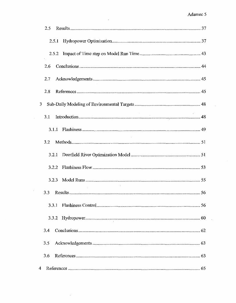
Contents

1 Optimization Modeling in the Deerfield Watershed .................................................... 8

1.1 Project Overview ................................................................................................... 8

1.2 Optimization Modeling ......................................................................................... 9

1.2.1 Linear Progrannning ..................................................................................... 10

1.2.2 Model Limitations ......................................................................................... 10

1.3 Literature Review ................................................................................................ 11

1.3.1 Optimization .................................................................................................. 11

1.3.2 Hydropower and Sub-Daily Time Steps ....................................................... 12

1.3.3 Environmental Impact ................................................................................... 13

1.4 The Deerfield Watershed ..................................................................................... 15

2 The Structure and Necessity of a Sub-Daily Model.. ................................................. 18

2.1 Introduction ......................................................................................................... 18

2.2 Background ......................................................................................................... 19

2.3 Deerfield River Optimization Model .................................................................. 20

2.3.1 Normalizing Objective Function Components .............................................. 24

2.3.2 Model Run Information ................................................................................. 26

2.3.3 Data Input for the Optimization Model... ...................................................... 27

2.4 Model Validation ................................................................................................. 32

2.4.1 Sub-Daily Model Verification ....................................................................... 36

Adamec5

2.5 Results ................................................................................................................. 37

2.5.1 Hydropower Optimization ............................................................................. 37

2.5.2 Impact ofTime step on Model Run Time ..................................................... 43

2.6 Conclusions ......................................................................................................... 44

2.7 Acknowledgements ............................................................................................. 45

2.8 References ........................................................................................................... 45

3 Sub-Daily Modeling ofEnviromnental Targets ......................................................... 48

3.1 Introduction ......................................................................................................... 48

3.1.1 Flashiness ...................................................................................................... 49

3.2 Methods ............................................................................................................... 51

3 .2.1 Deerfield River Optimization Model ............................................................ 51

3.2.2 Flashiness Flow ............................................................................................. 53

3.2.3 Model Runs ................................................................................................... 55

3.3 Results ................................................................................................................. 56

3.3.1 Flashiness Control ......................................................................................... 56

3.3.2 Hydropower ................................................................................................... 60

3.4 Conclusions ......................................................................................................... 62

3.5 Acknowledgements ............................................................................................. 63

3.6 References ........................................................................................................... 63

4 References .................................................................................................................. 65

Adamec6

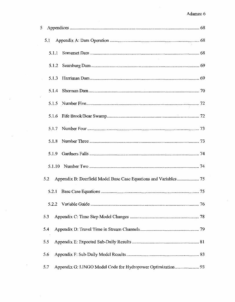
5 Appendices ................................................................................................................. 68

5.1 Appendix A: Dam Operation .............................................................................. 68

5.1.1 SomersetDam ............................................................................................... 68

5.1.2 Searsburg Dam .............................................................................................. 69

5.1.3 Harriman Dam ............................................................................................... 69

5.1.4 Sherman Dam ................................................................................................ 70

5.1.5 Number Five .................................................................................................. 72

5.1.6 Fife Brook/Bear Swamp ................................................................................ 72

5.1.7 Number Four ................................................................................................. 73

5.1.8 Number 1bree ............................................................................................... 73

5.1.9 Gardners Falls ............................................................................................... 74

5.1.10 Number Two ............................................................................................... 74

5.2 Appendix B: Deerfield Model Base Case Equations and Variables ................... 75

5.2.1 Base Case Equations ..................................................................................... 75

5.2.2 Variable Guide .............................................................................................. 76

5.3 Appendix C: Time Step Model Changes ............................................................ 78

5.4 Appendix D: Travel Time in Stream Channels ................................................... 79

5.5 Appendix E: Expected Sub-Daily Results .......................................................... 81

5.6 Appendix F: Sub-Daily Model Results ............................................................... 83

5.7 Appendix G: LINGO Model Code for Hydropower Optimization ..................... 93

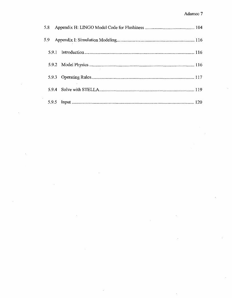
Adamec?

5.8 Appendix H: LINGO Model Code for Flashiness ............................................ 104

5.9 Appendix I: SimulationModeling ..................................................................... 116

5.9.1 Introduction ................................................................................................. 116

5.9.2 Model Physics ............................................................................................. 116

5.9.3 Operating Rules ........................................................................................... 117

5.9.4 Solve with STELLA .................................................................................... 119

5.9.5 Input ............................................................................................................ 120

Adamec8

1 Optimization Modeling in the Deerfield Watershed

1.1 Project Overview

This document is part of the Connecticut River Watershed Project, a federally authorized

collaborative project of the U.S. Army Corps of Engineers (US ACE), the Nature Conservancy

(TNC), the University of Massachusetts Amherst (UMass), and the U.S. Geological Survey

(USGS). The project began in September 2008 with Congressional funding for this project with

TNC and the USACE as equal funding partners.

The Connecticut River Watershed Project will identifY management modifications for

more than seventy influential dams in the Connecticut River Basin to increase environmental

benefits while maintaining beneficial human uses such as water supply, flood control, and

hydropower generation. Key project outcomes include a basin-wide simulation model and a

basin-wide, multi-objective optimization model. The optimization model will det=ine possible

environmental or hydropower benefits, explore coordinating release decisions, and explore best

operating decisions for specific objectives. More information regarding the UMass simulation

model can be found inAppendix I.

The models will provide numerous benefits. The models will allow water managers and

key stakeholders to evaluate environmental and economic outcomes based on various

management scenarios. They will inform flow recommendations that benefit both conservation

objectives and humans uses. They will enable the USACE to better manage its dams, providing

more natural stream flows while maintaining authorized flood control functionality. These tools

will also contribute to decision making for future Federal Energy Regulatory Commission

(FERC) licensing ofhydropower dams.

Adamec9

The basin-wide optimization model employs a daily time step. The Deerfield watershed,

a subset of the Connecticut River Basin, was selected to explore a sub-daily time step.

Differences in the output of the sub-daily time step model and the daily time step model provide

some insights into the value of increased temporal resolution. While providing beneficial

hydropower, Deerfield dams impact the natural hydrology of both the Deerfield River and lower

portions of the Connecticut River. Anafysis of the sub-daily model examines possible tradeoffs

between hydropower operations and meeting environmental targets.

1.2 Optimization Modeling

An optimization model provides insight into water resources systems problems by

explicitly defining the system and system performance objectives and by illustrating the trade

offs between these objectives. Optimization and simulation modeling methods are the primary

means of examining performance of particular water resources system designs and operating

policies (Loucks and van Beek 2005).

Optimization models determine the best solution for a system given specific model

objectives and constraints. Decision variables such as reservoir releases are calculated by the

optimization. Solving an optimization model finds "best" values for unknown decision variables

(Loucks and van Beek 2005).

Model objectives are expressions of system performance that can be either maximized or

minimized. One or more can be are combined in an objective function. The objective function

is the guiding statement of an optimization model. The contents of the objective function are

guided by quantitative measures of system performance.

Adamec 10

Constraints limit the value of decision variables, typically to reflect physical limitations

or operational limits. Variables in the optimization model must satisfY constraints. If there is no

solution that satisfies the constraints, the model is infeasible.

Targets express desired values of decision variables. Unlike constraints, targets are not

strictly enforced. A feasible solution can be found if a target is not satisfied. A minimum release

takes the form of a target. The model may not be able to meet a minimum release at all times,

but the release target is met whenever possible.

1.2.1 Linear Programming This investigation uses linear programming. Using a linear model allows very large and

complex problems to be solved, however, variables must be continuous and relationships must

be based on addition, subtraction, equality, and inequality. Linearization divorces the model

from what is in reality a nonlinear problem. Hydropower, for instance, is a nonlinear function of

both release and storage, by way ofhead. To linearize hydropower calculations within the

model, it is assumed that head remains constant at its maximum value. The optimization models

used here were developed in LINGO 11.0 from LINDO Systems, Inc.

1.2.2 Model Limitations The models in this thesis are ]:Jrovided with historic streamflow and cost of energy as

inputs. A disadvantage of linear programming is that these models assume perfect foresight of

future inflows and cost. This generates results that are typically superior to results achieved in

practice. Loucks and van Beek (2005) indicate that to compensate, optimization solutions should

be examined in detail and possibly assessed using simulation models. In some cases,

optimization models may be used for filtering clearly inferior solutions from feasible alternatives

(Loucks and van Beek 2005).

Adamec 11

1.3 Literature Review

1.3.1 Optimization Optimization modeling has a long history of application in the field of water resources,

and to reservoir operation in particular. Loucks and van Beek (2005) provide an introduction to

the application of optimization models to water resources systems. They describe the

components of optimization models as known input parameters, unknown decision variables, and

constraints. According to Loucks and van Beek (2005), "constrained optimization together with

simulation modeling is the primary way we have of estimating the values of the decision

variables that will best achieve specified performance objectives."

Wurbs (1991) describes the formulation of optimization models of reservoir systems,

providing detailed explanation of model variation due to various reservoir functions. Typical

reservoir functions include flood control, hydropower, water supply, and recreation. Wurbs

(1991) characterizes hydropower reservoirs as:

• hydropower storage, with large, long term storage that can be released at different

seasons or even different years;

• run of river, which, due to storage limitations or regulatory requirements, are limited so

that daily inflow is roughly equal to daily outflow (i.e. these reservoirs contain no active

storage); and

• pumped storage, where water is pumped to an upper storage reservoir during off-peak

energy prices and returned to generate power during peak load.

Y eh (1985) describes reservoir models in a 1985 state-of-the-art review. The review

covers a general overview of reservoir modeling, linear programming, dynamic programming,

noulinear programming, simulation, and several examples of operation models. Typical

Adamec 12

reservoir constraints mentioned here include continuity, maximum and minimum storage,

maximum and minimum releases, penstock limitations and contractual obligations. Optimization

and simulation models are differentiated as models that find optimum operations and models that

approximate system behavior. Optimization models are used for real time operation and

planning, while simulation models allow for exploration of consequences.

Labadie (2004) describes some of the more recent multi-reservoir optimization studies in

a state-of-the-art review. The concepts of implicit and explicit stochastic optimization, real time

optimization with forecasting, and heuristic progranuning are described and explored in recent

literature. Labadie (2004) mentions the gap between modeling technology and common model

implementation, forecasting hope that the gap will narrow.

Rani and Moreira (201 0) survey various approaches for reservoir systems operation

studies, including classical optimization modeling, simulation modeling, combined optimization

and simulation, and computational intelligence teclmiques such as evolutionary algorithms, fuzzy

set theory, and neural networks. Linear programming is discussed as one of the most popular

optimization teclmiques due to its flexibility, output of a global optimal solution, and the

availability of linear progranuning software. Disadvantages to linear progranuning include

restriction to linear convex objective functions and linear constraints. The paper discusses

current models that incorporate both simulation and optimization. Rani and Moreira (2010)

identifY future areas for reservoir modeling development including combined simulation and

optimization modeling and application of classical optimization teclmiques in conjunction with

computational intelligence teclmiques.

1.3.2 Hydropower and Sub-Daily Time Steps Models typically operate at a prescribed time step (hourly, daily, weekly, monthly

(Needham 2000; Alaya 2003; Hanscom et. al. 1980; Yeh et. al. 1979). For some applications,

Adamec 13

such as hydropower, a daily time step may not be sufficient to model desired system operations.

Hydropower operations typically account for hourly energy prices, and sub-daily releases are

made at the discretion of the dam owner or operator within the physical constraints of the

system.

1.3.3 Environmental Impact The intermittent flows typical ofhydropower generation cause negative downstream

effects. Bretschko and Moog (1990) demonstrate that the decline of natural flows occurs at a

much slower rate than that of unnatural hydropower flows. Increased damage due to

hydropower operations is attributed to the rapid rate of change of flow.

Parasiewicz et. a!. (1998) indicates that decreasing the ramping rate of hydropower

release mitigates the impacts on downstream communities of fish are mitigated. The paper refers

to other sources regarding hydropower peaking impacts on tail water communities of species

below hydropower dams. Particularly emphasized are the importance of peaking event

frequency and ramping rates caused by hydropower operations.

Poff (1997) introduces the concept of the natural flow regime. The paper emphasizes the

importance of natural streamflow variability. Instead of minimum flows, one view on

streamflow management sets reestablishing the natural flow regime as the goal for addressing

environmental concerns.

Richter and Thomas (2007) discuss the ecological impact of dams and make specific

recommendations for mitigation. Alteration of the natural flow regimes is identified as having

the most damaging effect on the river ecosystem and dependent flora and fauna. The goal for

mitigation is recognized as restoring natural flow regimes. Richter and Thomas (2007) make

observations about several different types of dams. Hydropower dams exhibit great capacity to

cause environmental damage, particularly by eliminating small floods, causing frequent pulses of

Adamec 14

artificiallrigh flow, or unnaturally lowering river levels. Large hydropower dams with the ability

to store a great deal of water have the most potential for damage. Releases from hydropower

dams are described as having a blocky hydrograph as dams use all available storage to capture

flood peaks and release and refill in cycles of hydropower generation. A primary mitigation

strategy for hydropower facilities include using downstream dams to reverse the unnatural flows

caused by hydropower dams. The paper proposes that cascades of reservoir in series,

particularly with little intervening river distance, are superior since the hydropower impact is

damage already done.

Jager and Bevelhimer (2007) examine the impact of reregulation on run of river dams,

noting that there was not a significant decrease in annual generation, although some of the

projects exlribited reduced efficiency or reduced release during peak demand. They note that run

of river operation tends to be minimal, so more effective ways to restore natural flow patterns are

to reregulate upstream hydropower peaking operations or restore natural flows with a storage

reservoir downstream of hydropower facilities.

Past environmental studies have included optimization. Harmon and Stewardson (2005)

use an optimization model to derive a rule curve for environmental flow releases. The

optimization results indicate the possibility of both water savings and meeting environmental

flow targets.

Jager and Smith (2008) review 29 hydropower decision analysis or optimization studies

that incorporate environmental criteria. They state that most major and some minor river

systems use optimization to identifY preferred release schedules. Results of tlris study indicate

that minimum flow constraints do not meet environmental needs. Jager and Smith (2008) predict

that further exploration of incorporating flow variability will be important in the future.

Adamec 15

Zimmerman et. al. (2009) explores sub-daily hydrologic alteration resulting from peaking

hydropower, run of river hydropower, and flood control dam operation. Mean daily flows can

mask sub-daily flow characteristics, so they calculate flashiness, or sub-daily flow variation, to

assess the impact of dam operations on sub-daily flow. Four metrics are used for flashiness: the

Richards-Baker (RB) index, the number of reversals, the percent of total flow, and the coefficient

of daily variation (CDV). As implemented in this paper, the RB index is the sum of the absolute

value of hourly total changes in hourly flows over the sum of hourly flows for each day. The

number of reversals is the number of changes between rising and falling periods for each day.

The percent oftotal flow is the difference between maximum hourly flow and minimum hourly

flow in a day divided by the total flow in the day. CDV is the standard deviation of hourly flows

in a day divided by mean daily flow. Zimmerman et. al. (2009) finds that while all rivers may

possess some degree of flashiness, rivers altered by dams experience notably more sub-daily

flow variability, particularly for peaking hydropower alteration.

1.4 The Deerfield Watershed

The USGS hydrologic unit code (HUC) 01080203defines the Deerfield watershed, the

region in which all water entering the system ultimately exits into the Connecticut River at the

mouth of the Deerfield River. The Deerfield watershed has a drainage area of approximately 665

square miles, 347 square miles in Massachusetts and 318 square miles in Vermont. Within the

watershed, the Deerfield River stretches approximately 70 miles from the Green Mountains in

Vermont, through the Berkshire Hills in Massachusetts, to the confluence with the Connecticut

River near Greenfield, Massachusetts. From its headwaters to its mouth, the river undergoes an

elevation drop of 2000 ·feet. Notable characteristics of the basin include rocky hills with shallow

bedrock and fairly well drained soils; narrow, steep-sided valleys; and shallow, rapidly-flowing

Adamec 16

mountain streams (FERC 1996). The basin is sparsely populated. Land use is primarily

deciduous and evergreen forests, as well as some agriculture around the Deerfield River and

major tributaries (FERC 1996).

The river itself is one of the most heavily used recreational rivers inN ew England (PERC

1996). Primary recreational uses are whitewater boating and angling (PERC 1996). Whitewater

boating typically occurs between Number 5 and Bear Swamp dams (Class IV or above

whitewater), and for about 5 miles below the Fife Brook dam (Class III whitewater) (PERC

1996). Angling includes lake fishing, often at Harriman reservoir (PERC 1996).

The Connecticut River Project focuses on dams selected by their hydropower generating

capacity, storage volume, and importance to the water system. There are eleven notable dams in

the Deerfield watershed, described in Table 1 and Figure 1. The Deerfield contains one dam for

storage, as well as hydropower storage dams, run of river hydropower dams, and pumped storage

dams. Most of these dams were constructed in the early 1900s (EOEA 2004).

Table 1: Reservoir Descriptions

Reservoir Storage Generating

Generating Drainage

Capacity Capacity Area Name

· (acre-ft) (MW) Head (ft)

(mi/\2)

Somerset 57345 -- -- 30 Sears burg 600 5 8 60 Harriman 318000 45 57.6 94

Sh=an 3593 6.4 11.6 50 Number Five 118 12 10 3 Fife Brook 4900 9 40 17 Bear Swamp 5260 580 730 --Number Four 467 6 5 150 Number Three 221 6 3 96 Gardners Falls 510 3.6 37 2 Number Two 550 6 11 3

0

.")

*Fiie!Brook

*~Number 4 .,{.:N4riJber ; ···*Gardners Falls'

. *Number 2.

Adamec 17

Figure 1: Dams in the Deerfield watershed, located in the Connecticut River Basin. Bear Swamp shares the same general location as Fife Brook.

Adamec 18

The facilities on the Deerfield River are licensed as three separate FERC projects. FERC

Project No. 2323, the Deerfield River Hydroelectric Project, contains Somerset, Searsbnrg,

Harriman, Sherman, Number 5, Number 4, Number 3, and Number 2. FERC Project No. 2669,

the Bear Swamp Pumped Storage Project, contains Bear Swamp and Fife Brook. FERC Project

No. 2334, the Gardners Falls Hydroelectric Project, contains Gardners Falls. Specifications and

operating information for each dam are detailed in Appendix A.

For the purpose of this investigation, the model neglects Bear Swamp since Bear Swamp

does not significantly change the operation of any other reservoir. The generating head at Bear

Swamp is significantly higher than at any other location, so Bear Swamp releases dominate

model outcome. Neglecting Bear Swamp emphasizes the operational changes introduced at the

other reservoirs.

2 The Structure and Necessity of a Sub-Daily Model

2.1 Introduction

Sub-daily hydropower releases are made at the discretion of the dam owner or operator

within the physical constraints of the system. Hydropower dam operators maximize income by

releasing water and generating hydropower when energy prices are high. As a result, sub-daily

fluctuation in the cost of energy is a major driving force behind release decisions at hydropower

dams.

A model that operates at a daily time step may generate different results than a model

which operates at a sub-daily time step. These differences can result in altered operational

patterns. This paper describes a linear optimization model of the Deerfield River operates on a

variety of temporal resolutions ranging from daily to hourly to explore the impact of model time

Adamec 19

step on results. Model implementation uses LINGO 11.0 from LINDO Systems, Inc. The model

imposes existing operational restrictions while otherwise allowing the model to maximize

income derived from hydropower.

The Deerfield watershed is located within the Connecticut River Basin, which extends

from northern New Hampshire through Vermont and Massachusetts to southern Connecticut,

where the Connecticut River releases into the Long Island Sound (Figure 1 ). Data for this

research draws from a larger project that incorporates the entire Connecticut River (Adamec et.

al. 2010; Pitta et. al. 2010). The Deerfield watershed contains ten hydropower generating dams

and one storage dam located along the Deerfield River. Each reservoir in the Deerfield has

physical information included in the model. These dams are described in Figure 1 and Table 1.

Fife Brook Dam forms the lower reservoir of a pumped storage facility. The model

neglects Bear Swamp, the upper reservoir of the pumped storage facility, since Bear Swamp does

not significantly change the operation of any other reservoir. The generating head at Bear

Swamp is significantly higher than at any other location, so Bear Swamp operates independently

of other Deerfield dams. Fife Brook has enough storage to make consistent releases over the

course of the day regardless of water removed to Bear Swamp, so Bear Swamp does not control

streamflows in the river. Neglecting Bear Swamp emphasizes the operational changes

introduced at the other reservoirs.

· 2.2 Background

Optimization modeling has a long history of application to the field of water resources,

and to reservoir operation in particular. Loucks and van Beek (2005) provide an introduction to

the application of optimization models to water resources systems. Wurbs (1991) meticulously

explains the formulation of optimization models of reservoir systems, providing detailed

Adamec20

explanation of model variation due to various reservoir functions. Yeh (1985) describes

reservoir models in a 1985 state-of-the-art review. Labadie (2004) describes some of the more

recent multi-reservoir optimization studies in a state-of-the-art review. Grygier and Stedinger

(1985) specify three strategies for deterministic optimization of hydropower operation.

Models assume a time step in which release decisions are made. Often this time step is

daily (Needham 2000) or monthly (Alaya 2003). Other studies use coupled models to aggregate

information at different time steps, including yearly, monthly, weekly and daily (Hanscom et. a!.

1980; Yeh et. a!. 1979). For applications such as hydropower, where there is incentive to have

sub-daily operational strategies, a model time step of a day or more may not be sufficient for

capturing system operations.

2.3 Deerfield River Optimization Model

The optimization model is formulated as a linear program. The objective function takes

the form:

N T

min I I ( -a1fJ1ln,t + az(fJzA~,t + {J3B~,t) + a3({J4AKt + fJsBJ:,t)) [1]

n=lt=l

where n is an index of reservoirs, t is an index of time, and ln,t is income, in dollars, at reservoir

n due to power generation over time step t. N is the total number of modeled reservoirs and Tis

the total number of modeled time steps. A~,t and B!:,t are storage target deviations and A~,t and

BJ{,t are release target deviations, in cubic feet (cf), during a time step. a1 , a 2 , and a3 are

normalization coefficients. {31 , {32 , {33 , {34 , and {35 are weight coefficients determined in model

calibration. The optimal solution to the model is the smallest value of Equation 1 that is possible

while satisfying Equations 2-14.

Adamec21

A mass balance equation describing system connectivity for storage at each reservoir is

written as,

Sn,t = Sn,t-1 + Qn,t - Rn,t [2]

Equation 2 states that storage, Sn,t' in reservoir n, at time period t, is equal to the sum of the

inflow entering each reservoir during a single time step, Qn,t' and the storage remaining in the

reservoir from the last time step, Sn,t-1 , minus the reservoir release during a single time step,

Rnt·

A simulation model of the system reveals that at the first day of the calendar year, each

reservoir in the Deerfield has a storage value approximately equal to the reservoir capacity,

Sn,max' so the initial storage of each reservoir, Sn,t=t> is set as the maximum operating storage

capacity of that reservoir,

Sn,t=1 = Sn,max = Sn,t=T [3]

Equation 3 also defines initial storage as final storage, Sn t=T' to prevent the model from draining

all reservoirs at the end of the operating horizon.

If an upstream reservoir exists, inflow is the sum of the upstream reservoir release and

calculated drainage accrued between the upstream reservoir and the reservoir in question, Dn,t·

If there is no upstream reservoir, inflow equals drainage above the reservoir. Reservoir inflow

for each time step is defined as

Qn,t = Dn,t + Rn-1,t [4]

where Rn=O t = 0.

Modeled release is separated into two components,

Adamec22

Rn,t = R~,t + R~,t [5]

where R~,t are releases that generate power and R~,t are releases that go directly to the river

without generating power. Hydropower dams direct water stored in an upstream reservoir

through a bypass or penstock to generate power via turbines housed within a powerhouse. It is

not always possible or pennissible to direct the total reservoir release to the turbines. R~ t

represents water released through the turbine. Spill or other release made directly to the river is

Income, In,t, is generated from R~,t and the price of energy for the time step in dollars per

megawatt-hour ($/MWh), Ct, via

ln,t = Ct * R~,t * hn,t * Y * 7J * \ji [6]

where hn,t is the head in feet at a dam at a given time step, y is 62.4 foot-pounds per second (ft-

lbs/s), 7J is the turbine efficiency, approximated as 0.9, and \ji is a conversion factor from ft-lbf"s

to MWh, equal to 1.356xlo·6. Multiplying release and a variable head forms a nonlinear

equation. Since Deerfield dams remain relatively full, head is approximated as a constant value

equal to the maximum dam height.

A physical limitation on reservoir storage takes the form

[7]

where Sn MIN is the minimum pennissible reservoir storage and Sn MAX is the maximum ' '

permissible reservoir storage.

Equations constraining direct releases between zero and a maximum direct release value,

R~ MAX and power releases between zero and a maximum power release value, R~ MAX are ' '

described as follows

Adamec23

0 ::; R~,t ::; R~,MAX [8]

0 ::; R~,t ::; R~,MAX [9]

Turbine or power generating capacity establishes R~ MAX.

Equation 1, the objective function, uses terms that express volume above and below

target minimum and maximum storage and release values. The methodology that yields these

terms is described by

s - E - iJE -BE n,t n,t - .n.n,t n,t [10]

sn,t - Fn,t = A~,t - BKt [11]

Rn,t - Gn,t = A~,t - B~,t [12]

Rn,t - Hn,t = A~,t - B;{,t [13]

Equation 10 yields A~,t, the volume for each time step by which the storage is above the

maximum storage target, En,t· Similarly, Equation 11 yields B~,t, the volume for each time step

by which the storage is below the minimum storage target, Fn,t· Equation 12 yields AKt, the

volume for each time step by which the release is above the maximum release target, Gn,t·

Equation 13 yields Bf:[ t, the volume for each time step by which the release is below the . '

minimum release target, Hn t· . '

Ramping is an expression of how much the release can change in a given amount of time.

A daily constraint on ramping in the model is imposed by

Adamec24

tz t4 tz

L Rn,t-1 - j ~ L Rn,t ~ L Rn,t-1 + k [14]

~G ~~ ~G

where t 1 is the first time step ofthe previous day, t 2is the last time step in the previous day, and

t 3 is the first time step in the current day, t 4 is the last time step in the current day,j is the

maximum permissible decrease in release over a single time period, and k is the maximum

permissible increase in release over a single time period. This constraint compares the sum of all

releases in a single day, even when the time step is less than daily. It is assumed that Rn,t=O = 0.

Appendix B summarizes the optimization model setup. Appendix G has LINGO code

implementation of the model.

2.3.1 Normalizing Objective Function Components Components in the objective function are normalized so that they may be compared

consistently and in a reasonable fashion. In this case, all decision variables are converted to a

value between 0 and 1. Normalization coefficients, a, and weight coefficients, p, are separated

in Equation 1 so that relative importance of decision variables can be assessed by comparing

weight coefficients. The following protocol describes the normalization used for storage targets,

release targets, and income in the Deerfield optimization model.

2.3.1.1 Income

Income in the optimization model is calculated by energy price, flow released through the

turbines, and the estimated head. Income is normalized by dividing the sum of the income

produced per time step by the maximum possible income, In,t,MAX, determined by assmning

maximum possible dam release and the 98'h percentile energy cost (81 $/MWh). This

normalized parameter has a maximum value very close to 1 and a minimum value of 0. This

Adamec25

parameter will be closer to 1 at each time step when more power is produced, but will typically

remain less than 1.

2.3.1.2 Storage Targets

1 al=--

In,t,MAX [15]

Each dam has an associated volume of impounded water that forms the reservoir storage.

Desired reservoir storages form targets in the model. Reservoir storage targets are normalized by

dividing the sum of storage target deviations at each time step by the maximum reservoir storage,

S, t MAX· Target deviation can never be greater than maximum storage or less than 0, so the

normalized parameter has a maximum value of 1 and a minimum value of 0 in each time step.

Deviation is 0 if a target is satisfied, so this parameter will preferably remain as close to 0 as

possible.

2.3.1.3 Release Targets

1 az = -=--

Sn,t,MAX [16]

Desired reservoir releases or downstream flows form release targets in the model.

Release targets are normalized by dividing the sum of release target deviations by the maximum

release, Rn,t,MAX. Target deviation can never be greater than maximum release or less than zero,

so the normalized parameter has a maximum value of 1 and a minimum value of 0 in each time

step. Deviation is 0 if a target is satisfied, so this parameter will preferably remain as close to 0

as possible.

1 a3=--

Rn,t,MAX [17]

Adamec26

2.3.2 Model Run Information The model runs for one calendar year, starting on the first hour of January 1 and ending

on the last hour of December 31. Storage is constrained so that initial and final storages are

equal, setting the volume of water entering each reservoir in a year equal to the volume of water

leaving each reservoir in the same year. Initial storages are defined as maximum reservoir

capacity for all reservoirs except Somerset. Somerset reservoir, with an operating maximum

elevation less than its capacity, is constrained similarly, where Ssomerset,t,max is defined as the

storage at the maximum operating elevation of2128.58 ft msL This constraint allows analysis of

seasonal variations in model results while placing logical boundary conditions on the final

storages to prevent unrealistic reservoir draw down at the end of the year.

Conditions specific to the Deerfield system make this constraint reasonable without a

large degree of alteration in model results. The total storage capacity of modeled Deerfield

reservoirs is 16,827 million cubic feet (386,304 acre-feet), over 1.6 times less than the total flow

through the model, 28,066 million cubic feet In reality, storage is further restricted by seasonal

constraints on reservoir release and storage. Since maximum total impoundment of water is less

than the volume of water transmitted through the watershed and seasonal limitations make it

more likely for Deerfield reservoirs to maintain relatively consistent storage volumes on the first

and last days of the year, the assumption of constant starting and ending storage is appropriate.

The optimization model is generalizable to any hourly or multiple of hourly time step.

Appendix C describes specific model changes. The model does not incorporate travel time from

one reservoir to the next nor is travel time imposed on drainage. Travel time between modeled

locations is considered sufficiently smalL Appendix D explores travel time and demonstrates

that including travel time has minimal impact on model results.

Adamec27

2.3.3 Data Input for the Optimization Model Historical streamflow and energy price data are used as model inputs. Streamflow is

derived from 1991 Instantaneous Data Archive (IDA) data at the USGS 01333000 Green River

Williamstown gage. Post -market hourly historical energy price data are obtained for 2000 from

ISO New England. The years of data that define the model input are different based on periods

ofbest data availability. Annual patterns are assumed to be sufficiently similar for this

exploration of sub-daily model structures.

2.3.3.1 Streamflow

Streamflow is derived from the Instantaneous Data Archive (IDA) data at the USGS

01333000 Green River Williamstown gage. The Williamstown gage and the nearby USGS

01170100 Green River Colrain gage are considered some of the least regulated gages in

Massachussetts (Armstrong 2008). In this case, unregulated gages refer to gages with little to no

upstream influence. Very few gages in Massachusetts and the New England region are

completely unaltered, but little alteration exists at the Williamstown and the Colrain gages.

The IDA contains streamflow recorded at 15 minute intervals. For many of the gages in

the region, the IDA streamflow contains missing days, sometimes up to a third of the year, and

collection times that are occasionally irregular. Missing days of data most likely result from ice

interfering with gage operation. Ice affects gage height data, which distorts the discharge

calculation. The IDA discards any day with ice. The Colrain gage data has between 35 and 106

missing days ranging in a year and contains both irregular and excess collection times. The

Williamstown gage data has 365 available days of data in the year 1991 with only one missing

hour. The two gages are similar to the Deerfield watershed in approximate geographical

proximity. They have similar drainage area sizes, are fairly mountainous, receive fairly

Adamec28

equivalent amounts of snow, and are mainly forested. The Williamstown gage was selected over

the Colrain gage due to data availability.

IDA 15 minute streamflow at the Green River Williamstown gage is averaged to an

hourly time step. The sole missing hour is approximated as the average value of the previous

and following hours. Hourly streamflow is averaged to 2, 3, 6, and 24 hours for other model

inputs. Streamflow inputs to each dam are approximated from Green River at Williamstown

streamflow by drainage area scaling.

Figure 2 shows the hydro graph of streamflow input used in the Deerfield optimization

model. The total volume of flow is 2.37xl 09 ft3 and the average daily flow is 75 cfs. Seasons

are defined as Winter (DJF), Spring (MAM), Summer (JJA), and Fall (SON). High flows occur

in Winter, Spring, and Fall, but rather than a consistently large flow, Fall flows have large storm

peaks.

~ " ~ ~

0 " ·" 0

"" "" c: "' " 0 ~

(!) 0

"' C> C> 0 <'> 0 <'>

"' 0

~ "" 0

1ii

~ 0 0

"" N

E "' " ~ i'il 0

Jan Feb Mar Apr May Jun Jul Aug Sept Oct Nov Dec

Month of 1991

Figure 2: Streamflow at the USGS Green River gage in 1991.

Adamec29

2.3.3.2 Energy Price

Energy prices vary over the course of the day based on demand (Figure 3). There is also

a seasonal variation in hourly energy price (Figure 4). Daily prices in particular increase

noticeably from Spring to Winter. Winter prices display the greatest distribution of prices.

Figure 4 and Figure 5 show that hourly maximum energy prices are greater than daily energy

prices and vary more widely. Sub-daily optimization models leverage the greater energy prices

available for short periods of the day by releasing as much as possible when prices are highest

0

"' ~

.c 0 s .... ::;;; e .,

0 • . g .,., "-61 ~

0 ., "' "' w <= :5 0 ., ::;;; ~

0

5 10 15 20

Hour of Day

Figure 3: Median energy price per day, calculated from 2000 ISO data

~

.c s 2 -<f> ~ ., (.)

·;:: 0.. :>. 2' ., <:: w

0 0 N

0 LO ~

0 0 ~

0 LO

~

' ' ' ' ' ' ' ' ' ' ' ' ' ' ' '

~ 0

' ' ~

Winter Spring

Adamec30

~ Daily Energy Price 0 D Hourly Maximum Energy Price

0

0

0 0

0

0 0 0 + 0 ~ ' ~ ' ' ' ' ' ' 0 ' 8 ' ' 0 ' 8 ' ~

' B B ~ ' ' ' ' ' ~ ~ ' ' ~ ' ' ~ ' -IT ' ' ~ ' ~

Summer Fall

Season

Figure 4: Distribution of daily energy price and hourly maximum price per day in 2000.

~

..<:: $: a -~ ~ Q) <> ·;:: 0.. :>. 0) '-Q) c IJJ

Legend

• Daily Energy Price

Adamec31

~ A Hourly Maximum Energy Price

0 0 "<~"

fj,

fj,

0 0

'"

0 0 N b.

fj, fj,

A {>. fj,


Month of 2000

Figure 5: Daily energy prices and maximum hourly energy prices for each day in 2000.

Energy price is the price at which energy is sold. Energy price reflects the energy

demand of the market. Hydropower reservoirs generate energy when the demand of the energy

market is greatest by timing releases to match periods of high energy prices to produce more

income. Matching reservoir releases with high energy prices increases the satisfaction of energy

demand. ISO New England provides price of energy information in units of dollars per

Adamec 32

megawatt-hour available on an hourly basis. Post-market hourly historical energy price data are

available from mid-1999 to mid-2003. This paper uses energy prices from the calendar year

2000. These data are considered representative of the variability seen in hourly energy prices

over an annual period.

2.4 Model Validation

Once constructed, models are validated by comparing modeled results to historic data.

Optimization modeling approximates reality to a degree, dependent on model input, objective

function components and weights, and model constraints. The model input draws from 1991 and

2000 rather than directly corresponding to a single specific year of record and the perfect

knowledge of the future that the optimization model possesses did not exist historically. Instead

of matching a specific historical year, the model is considered accurate if modeled results

generally follow the historical trend.

The optimization model is validated by comparing model results with existing historical

storage data at Somerset and Harriman. Figure 6 and Figure 7 present modeled storages in bold

along with historical storages from 2000 to 2009 at two of the larger dams, where storage data is

available. In both cases, modeled storages begin and end slightly higher than the historical

record. The model storages are derived from maximum storage capacities or maximum

operating levels. While initial and final storages are fixed, modeled storage patterns are similar

to historical at the beginning and towards the end of the year and the compliance with the loon

nesting storage target at Somerset, indicating that storage at Somerset and Harriman are

following the historical trend.

Adamec 33

0 0 0 0

"' ~

¢' 0 ' 0

<ll 0 ~ 0 0

~ "' <ll

"" 0 r: 0 0 0 - 0

{{) ~ -<ll Ul 0 ~

<ll 0 E C> 0 0

{{) "" 0 C> 0 0 N


Month of Year

Figure 6: Storage at Somerset. Storage derived from the optimization model run at a daily time step (bold) is plotted with storage at each year from 2000 to 2009 (dashed).

0 0 0 0

~

Jan Feb Mar Apr May Jun Jul

Month of Year

Aug Sept Oct Nov Dec

Figure 7: Storage at Harriman. Storage derived from the optimization model run at a daily time step (bold) is plotted with storage at each year from 2000 to 2009 (dashed).

Adamec34

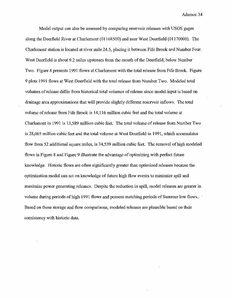
Model output can also be assessed by comparing reservoir releases with USGS gages

along the Deerfield River at Charlemont (01168500) and near West Deerfield (01170000). The

Charlemont station is located at river mile 24.5, placing it between Fife Brook and Number Four.

West Deerfield is about 9.2 miles upstream from the mouth of the Deerfield, below Number

Two. Figure 8 presents 1991 flows at Charlemont with the total release from Fife Brook. Figure

9 plots 1991 flows at West Deerfield with the total release from Number Two. Modeled total

volumes of release differ from historical total volumes of release since model input is based on

drainage area approximations that will provide slightly different reservoir inflows. The total

volume of release from Fife Brook is 14,116 million cubic feet and the total volume at

Charlemont in 1991 is 13,589 million cubic feet. The total volume of release from Number Two

is 28,065 million cubic feet and the total volume at West Deerfield in 1991, which accumulates

flow from 52 additional square miles, is 34,539 million cubic feet. The removal of high modeled

flows in Figure 8 and Figure 9 illustrate the advantage of optimizing with perfect future

knowledge. Historic flows are often significantly greater than optimized releases because the

optimization model can act on knowledge of future high flow events to minimize spill and

maximize power generating releases. Despite the reduction in spill, model releases are greater in

volume during periods of high 1991 flows and possess matching periods of Summer low flows ..

Based on these storage and flow comparisons, modeled releases are plausible based on their

consistency with historic data.

~ .:e ~ 0 c: 0

0 0 .... "' ·c "' 0 0. 0 E 0 0 <'>

0 0

~ 0 0

u.. "' c 0 0 8-E " -iij 5 0

Legend

Charlemont Daily Model Release

Adamec35

l, : l

~~~~~ ' ' ' ' ' '


Month of Year

Figure 8: Model release from Fife Brook is plotted with historical flow at Charlemont in 1991.

~ .:e 0 0 ~ 0 c 0 0 N

·! -"' Q.

E 0 0 0

0 0

~ "' u:: 32 0

0

" 0 'E .... " "' 0

'lh 0

~

Legend

West Deerfield Daily Model Release

!l ll

II

~~. Jan Feb Mar Apr May Jun Jul

Month of Year

Aug Sept Oct Nov Dec

Figure 9: Model release from Number Two is plotted with historical flow near West Deerfield in 1991.

Figure 10 shows how the optimization model reacts to a high flow event Modeled

reservoir storages are drawn down in anticipation of the flood event around day 230. When the

flood occurs, instead of spilling, reservoirs are able to capture the flood with minimal spilL

Number Two and Gardners Falls illustrate the reactions of the two closest dams, while Fife

Adamec36

Brook demonstrates that even the behavior oflarger upstream dams adjusts to accommodate

storm peaks.

~

"" • ., ~

"' ~ ., Ol E 0 ti5

0 0 0

"'

0 0 LO ~

0 0 0 ~

0 0 LO

0

8/1

legend

West Deerfield storm Event Number 2 Storage Gardners Falls storage Fife Brook Storage

J - l I l

8/10

I I

r----,

-- I

I I

' l l v.: ___ _ \ I \I

I l ' I

l \

J I

I-

I I

''\ I

~· ""······· L------................ ·-·-···-······'··--·········-··--·

8120

Day of Year

8/30

Figure 10: Storage draw down in anticipation of a high flow event.

2.4.1 Sub-Daily Model Verification To evaluate model runs at various sub-daily time steps the model is tested with

constraints designed to render the sub-daily model logically equivalent to the daily model.

0 0 0

"'

0 0 0

""

0 0 0 '<!"

0 0 0

"'

0

~

.:2 <.> -"' 0

q:: E

"' "' ~ -(/)

Direct and power releases at each reservoir are set equal to the direct and power releases at every

other time step within a given day. Inflows to each reservoir are set as proportions of average

daily inflow per time step. Ramping, as indicated in Equation 14, is calculated as the change in

release from one day to the next, regardless of time step. Thus, ramping should not differentiate

Adamec 37

daily and sub-daily models. Models are compared both with constant energy price for each time

step within a day and for varying sub-daily energy prices that average to the daily energy price.

In this constrained form, sub-daily models have equivalent storage and release values to

daily models. Average daily storage values computed from sub-daily storages are compared

with daily storage values and cumulative daily release values computed from sub-daily releases

are compared with daily release values. Daily and sub-daily models have matching storage and

release val?es, so the models are considered equivalent.

2.5 Results

Analysis of sub-daily models involves comparing them to a daily model. Generally,

comparison involves sub-daily results that are aggregated to daily results. Sub-daily models are

compared with daily models by examining the difference of release and revenue on a daily,

monthly, and seasonal basis.

2.5.1 Hydropower Optimization To explore the impact of time step on optimal hydropower operation, the Deerfield Base

Case model without travel time is optimized for 1, 2, 3, 6, and 12 hour time steps. Differences in

modeled income indicate operational modifications due to varying model resolutions. The

income generated at all of the modeled hydropower dams for one year is presented in Figure 11.

0 0 0 ci

e

12-.,.,

"' "' "' 0

"' "'

Adamec 38

• •

•

•

•

• '

1 2 3 4 5 6 7 8 9 10 11 12 13 14 15 16 17 18 19 20 21 22 23 24

#Time Steps per Day

Figure 11: Yearly income for models of different time steps

Figure 11 indicates that, as expected (see Appendix E), optimized income increases with

increasing model time step. The relationship between number of time steps pef day and total

model income is not linear. Reducing the time step from one day to 12 hours or 6 hours creates a

more significant increase in model income than reducing the time step from 2 hours to 1 hour.

The total increase in income gained from reducing the time step from a day to 1 hour is

approximately $318,000, an 8.6% increase and an order of magnitude less than the income

generated at 1 hour. Table 2 similarly indicates that more income is generated as model

resolution increases. Desired resolution of the model still depends on the desired level of

accuracy, but these results indicate that increasing the model resolution will lead to ·more income

generated by the optimization model.

Adamec39

Table 2: Total model income for months and seasons in nnits of million dollars

Model Time Step lncome [1 OA6 $] Daily 12Hr 6Hr 3Hr 2Hr Hourly

Monthly January 0.408 0.411 0.404 0.401 0.403 0.403

February 0.332 0.335 0.328 0.333 0.330 0.334

March 0.106 0.116 0.137 0.146 0.149 0.150

April 0.158 0.163 0.184 0.186 0.192 0.190

May 0.767 0.777 0.805 0.807 0.807 0.811

June 0.114 0.141 0.135 0.154 0.152 0.155

July 0.014 0.048 0.055 0.075 0.079 0.082

August 0.167 0.178 0.194 0.194 0.193 0.199

September 0.130 0.141 0.154 0.160 0.166 0.162

October 0.406 0.371 0.359 0.345 0.352 0.353

November 0.242 0.244 0.274 0.279 0.276 0.280

December 0.518 0.527 0.541 0.549 0.557 0.557

Seasonally Winter 1.776 1.799 1.814 1.831 1.846 1.851

Spring 1.031 1.057 1.127 1.139 1.148 1.151

Summer 0.295 0.368 0.384 0.424 0.425 0.436

Fall 0.778 0.755 0.787 0.784 0.794 0.795

Yearly 3.362 3.453 3.571 3.630 3.656 3.677

Adamec40

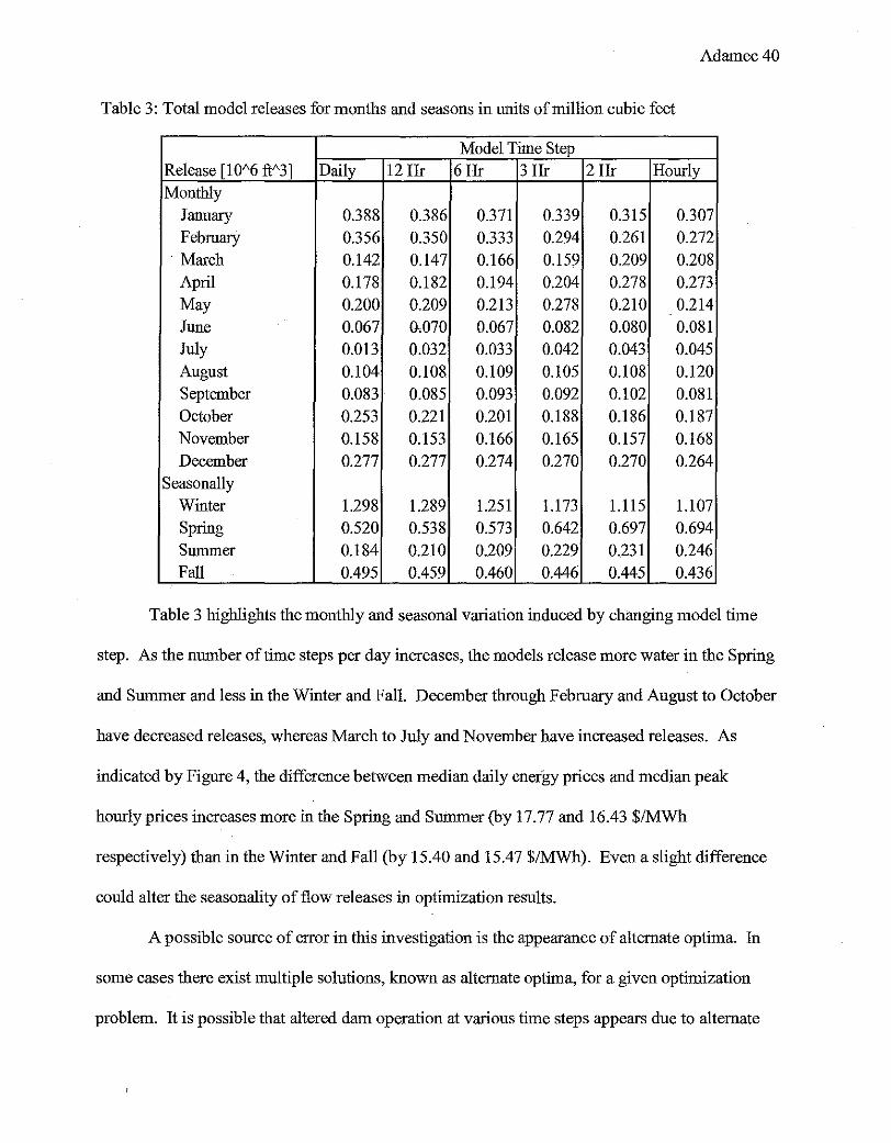
Table 3: Total model releases for months and seasons in units of million cubic feet

Model Time Step Release [10"6 ft"3] Daily 12Hr 6Hr 3Hr 2Hr Hourly Monthly

January 0.388 0.386 0.371 0.339 0.315 0.307 February 0.356 0.350 0.333 0.294 0.261 0.272

·March 0.142 0.147 0.166 0.159 0.209 0.208 April 0.178 0.182 0.194 0.204 0.278 0.273 May 0.200 0.209 0.213 0.278 0.210 0.214 June 0.067 omo 0.067 0.082 0.080 0.081 July 0.013 0.032 0.033 0.042 0.043 0.045 August 0.104 0.108 0.109 0.105 0.108 0.120 September 0.083 0.085 0.093 0.092 0.102 0.081 October 0.253 0.221 0.201 0.188 0.186 0.187 November 0.158 0.153 0.166 0.165 0.157 0.168 December 0.277 0.277 0.274 0.270 0.270 0.264

Seasonally Winter 1.298 1.289 1.251 1.173 1.115 1.107 Spring 0.520 0.538 0.573 0.642 0.697 0.694 Smmner 0.184 0.210 0.209 0.229 0.231 0.246 Fall 0.495 0.459 0.460 0.446 0.445 0.436

Table 3 highlights the monthly and seasonal variation induced by changing model time

step. As the number of time steps per day increases, the models release more water in the Spring

and Summer and less in the Winter and Fall. December through February and August to October

have decreased releases, whereas March to July and November have increased releases. As

indicated by Figure 4, the difference between median daily energy prices and median peak

hourly prices increases more in the Spring and Summer (by 17.77 and 16.43 $/MWh

respectively) than in the Winter and Fall (by 15.40 and 15.47 $/MWh). Even a slight difference

could alter the seasonality of flow releases in optimization results.

A possible source of error in this investigation is the appearance of alternate optima. In

some cases there exist multiple solutions, known as alternate optima, for a given optimization

problem. It is possible that altered dam operation at various time steps appears due to alternate

Adamec41

optima rather than meaningful changes in operation strategy. The consistency of trends in Table

2 and Table 3 indicate that the differing results of various resolution models are patterns rather

than alternate optima strategies.

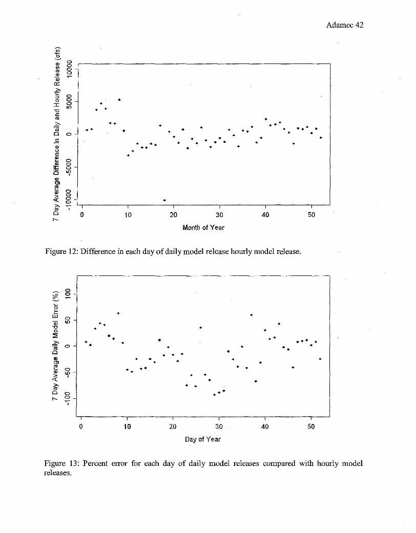
Figure 12 and Figure 13 illustrate the difference between the daily and hourly

optimization models. Plotting the 7 day average difference in each day of volume released in the

daily model and volume released in the hourly model shows that the model output varies

noticeably by over 5000 cfs in either direction. In the Summer, there are some periods in which

differences are relatively small, explained by the limitation oflow Summer inflows. Percent

error in Figure 13 is calculated by the difference between hourly model release and daily model

release in a day divided by hourly model release in a day. Figure 13 highlights that the daily

model more commonly releases less than the hourly model, but when the daily model releases

more that the hourly model, it releases significantly more. This behavior is in line with the

expectation that the daily model will respond with larger releases to days with high energy

prices, but days with high hourly energy prices and low average energy prices will elicit a

diminished response from the daily model.

~ ~ ., 0

"' g_ .. Q) 0 a; ~

0:::

£ 0 ::>

0 g. • :c • "" • • v

<::

"' • ;c. •• • • • • • • ••• "(ij •• • • • • 0 • • • • • • 0 • • . 5 • • • •

• •• • • • • • • "' •• • • • 0 • <:: • ~ 0

"' 0 !!: 0 Cl "' ' "' Ol .. ~ 0 "' ~ 0 g- • "' ~ ' ' l l

"' ' Cl 0 10 20 30 40 50 ,_ Month of Year

Figure 12: Difference in each day of daily model release hourly model release .

0

•• •

• •

•

• • •

• • • ......

10

• •

• • • •

20

•

• • •

• • •• •

30

Day of Year

•

• • •

• • • • •

•

l

40

•

• •

•

• ••• •

' 50

Adamec42

•

•

Figure 13: Percent error for each day of daily model releases compared with hourly model releases.

Adamec43

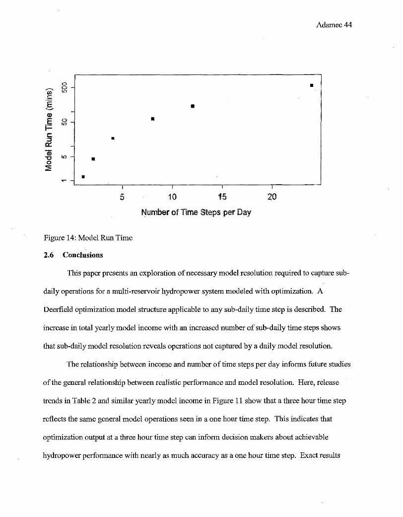
2.5.2 Impact of Time step on Model Run Time While a greater model resolution presents a more accurate representation of aetna!

operational abilitY, model time steps are often intentionally large. Models with more time steps

have more decision variables than models with fewer time steps. Table 4 shows that as model

time step increases from daily to hourly, the number of model variables increases from 4.7x1 04

to 113.0x104• In an optimization model, adding more time steps increases the number of

necessary computations and thus the model run time. Figure 14 demonstrates how model run

time increases significantly when more time steps are computed per day. When determining

acceptable model time step, both acceptable model resolution determined from Figure 11 and

concerns such as model run time and data availability should be taken into accOtmt.

Table 4: Model variables for different model lengths

Time Step Time Model Constraints

(hrs} Steps/Day T

Variables

24 1 365 47132 41974 12 2 730 94217 76649

6 4 1460 188387 145999 3 8 2920 376727 284699 2 12 4380 565067 423399 1 24 8760 1130087 839499

Adamec44

0 ~ g-fJ>

• £ E • ._,

-(!)

E :5- • F c: • :::J

0:: -"li)

ID-'"t:l • 0 ::2:

• ~

' ' I

5 10 15 20

Number of Time Steps per Day

Figure 14: Model Run Time

2.6 Conclusions

This paper presents an exploration of necessary model resolution required to capture sub-

daily operations for a multi-reservoir hydropower system modeled with optimization. A

Deerfield optimization model structure applicable to any sub-daily time step is described. The

increase in total yearly model income with an increased number of sub-daily time steps shows

that sub-daily model resolution reveals operations not captured by a daily model resolution.

The relationship between income and number of time steps per day informs future studies

of the general relationship between realistic performance and model resolution. Here, release

trends in Table 2 and similar yearly model income in Figure 11 show that a three hour time step

reflects the same general model operations seen in a one hour time step. This indicates that

optimization output at a three hour time step can inform decision makers about achievable

hydropower performance with nearly as much accuracy as a one hour time step. Exact results

Adamec45

may be specific to the Deerfield watershed, but this study has demonstrated both a requirement

of finer resolution to capture hydropower operations and the existence of a time step greater than

hourly that closely approximates hourly results.

While the hydropower optimization model used here did not include travel time, the sub

daily modeling structure is applicable to a model that includes travel time. As demonstrated,

travel time does not strongly influence results derived in this study. Travel time may need to be

accommodated in other study areas and should not be discounted.

In this exploration, input was selected from available records. Further modeling efforts

could focus on a single historical year or take a different approach to establishing model inflows.

A sub-daily model constructed in the manner of the Deerfield model described-here could

incorporate climate impacted streamflows as alternate inflows, change the weighting and

normalization of objectives within the model, and change allocation of water between power

generation bypass and direct discharge to the river. Using a sub-daily model, one could form

operational suggestions for selected scenarios, including analysis of increasing minimum flows

or installation of more generating capacity.

2.7 Acknowledgements

This project was part of the Connecticut River Watershed Project, a joint partuership of

The Nature Conservancy and the U.S. Army Corps of Engineers. Funding for this project was

provided by TheN ature Conservancy.

2.8 References

Adamec, K., Pahner, R.N., Polebitski, A., Ahlfeld, D., Steinschneider, S., Pitta, B., and

Brown, C. (20 1 0). Evaluation of climate change impacts to reservoir operations within the

Adamec46

Connecticut River Basin. In R.N. Palmer (Ed.) World Environmental and Water Resources

Congress 2010: Challenges of Change. Reston, VA: ASCE.

Alaya, A.B., Souissi, A, Tarhouni, J., and Ncib, K. (2003). Optimization ofNebhana

Reservoir Water Allocation by Stochastic Dynamic Programming. Water Resources

Management, 17, 259-272.

Armstrong, D.S., Parker, G.W., and Richards, T.A., 2008, Characteristics and

classification ofleast altered streamflows in Massachusetts: U.S. Geological Survey Scientific

Investigations Report 2007-5291, 113 p., plus CD-ROM.

Grygier, J.C., and Stedinger, J.R. (1985). Algorithms for optimizing hydropower system

operation. Water Resources Research, 21(1), 1-10.

Hanscom, M.A., Lafond, L., Lasdon, L., and Pronovost, G. (1980). Modeling and

resolution of the medium term energy generation planning problem for a large hydro-electric

system. Management Science, 26(7), 659-668.

Labadie, J.W. (2004). Optimal Operation ofMultireservoir Systems: State-of-the-Art

Review. Journal of Water Resources Planning and Management, 130(2), 93-111.

Loucks, D.P. and van Beek, E. (2005). Water Resources Systems Planning and

Management: An Introduction to Methods, Models, and Applications. The Netherlands:

UNESCO Publishing.

Needham, J.T., et. al. (2000). Linear Programming for Flood Control in the Iowa and Des

Moines Rivers. Journal of Water Resources Planning and Management, 126(3), 118-127.

Pitta, B., Palmer, R., Adamec, K., Polebitski, A, and Steinschneider, S. (2010).

Optimizing reservoir operations in the Connecticut River Basin. In R.N. Palmer (Ed.) World

Adamec47

Environmental and Water Resources Congress 20 I 0: Challenges of Change. Reston, VA:

ASCE.

Wurbs, R.A. (1991). Optimization of Multiple-Purpose Reservoir System Operations: A

Review of Modeling and Analysis Approaches. US Army Corps of Engineers: Hydrologic

Engineering Center. Research Document No. 34.

Yeh, W.WG. (1985). Reservoir Management and Operations Models: A State-of-the-Art

Review. Water Resources Research, 21(12).

Yeh, W.WG. Becker, L., and Chu, W-S. (1979). Real-time hourly reservoir operation.

Journal of the Water Resources Planning and Management Division, 105(2), 187-203.

Adamec48

3 Sub-Daily Modeling of Environmental Targets

3.1 Introduction

Optimization models determine the best solution for a system given specific model

objectives and constraints. Model objectives are expressed in a maximizing or minimizing

statement known as an objective function that the model solves. Constraints are limiting

expressions that must be upheld in the model solution. Optimization modeling of reservoir

systems allows decision makers to examine tradeoffs between multiple objectives. Jager and

Smith (2008) state that most major and some minor river systems use optimization to identify

preferred release schedules.

Optimization modeling is a component of many past environmental studies. Jager and

Smith (2008) review 29 hydropower decision analysis or optimization studies that incorporate

environmental criteria. A typical approach to addressing environmental needs is by setting

minimum flow constraints. With this approach, optimization for environmental targets examines

operating alternatives that balance minimum flow constraints and the current demands on the

water system. Harmon and Stewardson (2005) use an optimization model to derive a rule curve

for environmental flow releases. Minimum flow constraints do not satisfy environmental

concerns (Jager and Smith 2008). While minimum flows may supply a necessary volume of

water, they do not guarantee flow patterns necessary for habitat formation.

Instead of minimum flows, one view on streamflow management sets reestablishing the

natural flow regime as the goal for addressing environmental concerns. Poff (1997) highlights

the importance of natural streamflow variability. Jager and Smith (2008) predict that further

exploration of incorporating flow variability will be important in the future. An hourly

optimization model of reservoir releases on the Deerfield River provides the means to explore

Adamec49

the restoration ofhourly flow variability. Adamec (20 11) (i.e. Chapter 2) describes the model

construction in detail.

The Deerfield watershed is a subset of the Connecticut River basin located in

northwestern Massachusetts and southern Vermont. There are ten modeled reservoirs in the

Deerfield watershed including one storage reservoir, and the lower reservoir of a pumped storage

facility. Figure 1 describes the dam locations within the Deerfield watershed. While providing

beneficial hydropower, these dams influence the natural hydrology of the Deerfield River and

lower portions of the Connecticut River. Hydropower dams have the potential to cause

environmental damage by eliminating small floods, causing frequent pulses of artificial high

flow, or unnaturally lowering river levels (Richter and Thomas 2007). Analysis of the sub-daily

model will examine possible tradeoffs between hydropower operations and environmental targets

based on the natural flow regime.

3.1.1 Flashiness Flashiness is a characteristic of the flow in a stream. Past literature provides alternate

definitions of flashiness. Baker et.al. (2004) describes flashiness as the frequency of short term

streamflow changes, noted as especially relevant to runoff events and land use changes. Poff

(1997) defines flashiness as the rate of change in flow. Zimmerman et.al. (2009) characterizes

streamflow gages as "flashy" and "non-flashy" based on thresholds of subdaily variation.

Flashiness here refers to sub-daily flow variability.

Flashiness is part of the natural flow regime of the Deerfield River. Steep slopes and

shallow soil depth to bedrock in the upper portion of the watershed contribute to rapidly

changing flows in the river (FERC 1996). Flows regulated by the hydropower peaking dam

operations of Deerfield dams have significantly altered the natural flow regime. Hydropower

peaking operations result in large releases during peak power demands in order to maximize

Adamec 50

income from power generation. Hydropower operation typically creates intermittent flows

which exhibit much more rapid declines than natural flows (Bretshko and Moog 1990).

Streamflow flashiness due to hydropower operation results in the most environmentally

damaging downstream effects of hydropower dams.

The Deerfield River provides habitat to a number of fish species, most notably the

Atlantic sahnon. Atlantic salmon are stocked in the Deerfield River as part of the Atlantic

Salmon Restoration Program, so environmental factors affecting Atlantic salmon are of

particular concern. Flashiness disturbs the ecosystem and can be especially damaging to sahnon

dUring migration and spawning. Parasiewicz et. al. (1998) indicates that the impacts on

downstream communities offish are mitigated by decreasing the ramping rate of hydropower

release. Environmental targets for the Deerfield are improved by decreasing unnatural flashiness

in the river.

Flashiness can be quantified in a variety of ways. Zimmerman et.al. (2009) suggests

using the Richards-Baker (RB) index, the number of reversals, the percent of total flow, and the

coefficient of daily variation (CDV). The number of reversals is the number of changes between

rising and falling periods for each day. The percent of total flow is the difference between

maximum hourly flow and minimum hourly flow in a day divided by the total flow in the day.

CDV is the standard deviation of hourly flows in a day divided by mean daily flow. Other

flashiness metrics exist, such as the number of days per year above mean daily flow, but the RB

index is the predominant metric and is the focus of modeling efforts in this paper involving

flashiness in the sub-daily model.

Adamec 51

As implemented by Zimmerman et.al. (2009), the RB index is the sum of the absolute

value of hourly total changes in hourly flows over the sum of hourly flows for each day. The RB

index is described by Equation 18,

[18]

where Rn t is the hourly flow volume at reservoir n in hour t, t is an index of the hour of day, and

t+23 sets the summation to span 24 hours, the total number of hours per day. Note that, as

originally established, the Richards-Baker index was typically applied to daily variation over a

year, where Rn t is daily flow and the numerator and denominator are summed over the number

of days in a year (Baker 2004).

Zimmerman et.al. (2009) quantifies flashiness by measuring the number of days per year

that the RB index exceeds 0.05. The value 0.05 was selected based on data from reference gages

as the approximate inflection point above which daily streamflow may be considered flashy.

Mean number of days exceeding aRB index of 0.05 were 32 for unregulated sites, 31 for sites

with flood control regulation, 67 for sites run of river hydropower regulation, and 202 for sites

with hydro peaking regulation, based on calculations at selected USGS. Downstream of the

modeled Deerfield dams at the West Deerfield USGS gage (01170000), the Deerfield River

exceeded 0.05 on an average of221 days per year. These values found by Zimmerman et. a!.

(2009) create a frame of reference for RB index exceedance.

3.2 Methods

3.2.1 Deerfield River Optimization Model Analysis of flashiness is based on the linear optimization model defined as follows:

Adamec 52

N T

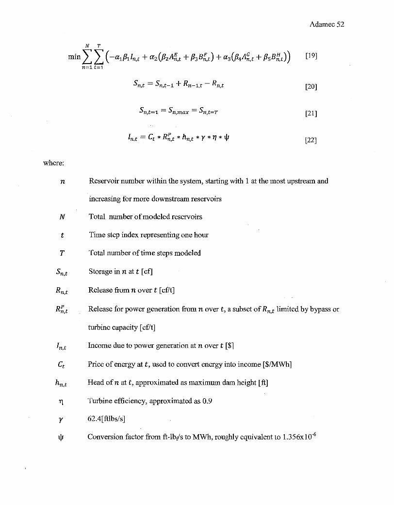
min I I ( -a1/Mn,t + az(PzA~,t + P3Bh_t) + a3(p4~,t + PsB;{,t)) [19]

n:::::lt=l

[20]

Sn t=l = Sn max = Sn t=T ' ' ' [21]

ln,t = Ct * Rh,t * h.n,t * Y * 1J * \fJ [22]

where:

n Reservoir number within the system, starting with I at the most upstream and

increasing for more downstream reservoirs

N Total number of modeled reservoirs

t Time step index representing one hour

T Total number oftime steps modeled

Sn,t Storage in n at t [ cf]

Rn t Release from n over t [ cf/t]

Rh,t Release for power generation from n overt, a subset of Rn,t limited by bypass or

turbine capacity [ cflt]

In t Income due to power generation at n over t [$]

Ct Price of energy at t, used to convert energy into income [$/MWh]

h.n,t Head ofn at t, approximated as maximum dam height [ft]

11 Turbine efficiency, approximated as 0.9

y 62.4[ ftlbs/s]

\fl Conversion factor from ft-lbls to MWh, roughly equivalent to 1.356xl0-6

Adamec 53

A~,t Volume for each t by which the storage is above the maximum storage target

B~,t Volume for each t by which the storage is below the minimum storage target

A~,t Volume for each t by which the release is above the maximum release target

Bi{ t Volume for each t by which the release is below the minimum release target

a Normalization coefficient

fJ Weight coefficient

For this model, at. a2 , and a 3 are normalization coefficients. {11 , {12 , {13 , {14 , and {15 are

weight coefficients determined in model calibration. Storage and release values are limited

based on maximum and minimum permissible levels. Appendix H has LINGO code

implementation of the modeL

Input streamflow is derived from the Instantaneous Data Archive (IDA) data at the USGS

01333000 Green River Williamstown gage for 1991. Price of energy information is available

from ISO New England in units of dollars per megawatt-hour available on an hourly basis. As

the closest year to 1991 with a complete record, hourly energy price information from the year

2000 is used to calculate income in the model.

3.2.2 Flashiness Flow Flashiness is incorporated into the Deerfield optimization model to explore the tradeoff

between income due to hydropower generation and environmental concerns. The flashiness

quantification described in Zimmerman et. a!. (2009) presents the number of days in which the

RB index exceeds a given value as a standard for environmental improvement. Evaluating a

yearly number of values assessed daily within an hourly optimization model is computationally

challenging when using an LP model. Attaining a desired number of exceeded days in a year is a

Adamec 54

complex process. Instead, the hourly model uses an intermediate flashiness flow to impose

flashiness restrictions as ramping constraints.

A flashiness ramping constraint imposes a constraint on the volume of water by which

release at each reservoir is permitted to increase or decrease from release in the previous time

step. The flashiness flow is this maximum change in hourly flow, as seen in Equation 23,

Rnt-1- FF < Rnt < Rnt-1 + FF ' ' ' [23]

Where PP is flashiness flow and Rn,t represents the release at a reservoir, n, in a model hour, t.

The RB index in Equation 18 is modified to form the flashiness flow used in Equation 25.

Modifications to Equation 18 make assumptions that are inconsistent with the RB index

definition. The RB index term is replaced by a flashiness index, PI, which is similar to the RB

index, but permits the modification assumptions. PI is determined from the desired number of

days in which the RB index exceeds a specified value.

Each term in the numerator of Equation 18 is the average magnitude of the change in

flow before and after each hour of a day. The ramping constraint imposes a maximum change

limitation, so the change in flow from hour to hour is assumed to be constant and at its greatest

magnitude for the calculation of flashiness flow. This term takes the constant value of 24 times

the maximum hourly flow.

The denominator of Equation 18 is total daily flow. To calculate the flashiness flow at

reservoir n, each term in the denominator is set equal to the sum of daily inflow at the given

reservoir and all reservoirs upstream, referred to as NDP. This quantity is an estimation of

natural daily flow with no time delay or regulation. The natural daily flow simulation term,

NDP, allows the flashiness flow to account for naturally occurring high and low flows.

Adamec 55

Enforcing with a FF based on simulated natural flow brings releases closer to the natural flow

regime while isolating and limiting flashiness due to hydropower.

With these assumptions in place, Equation 18 can be rewritten as follows:

FF * 24 FI = --=-==

NDF

Solving for the FF yields Equation 25:

FI FF=-*NDF

24

Equation 25 provides the FF ramping term used in Equation 23.

3.2.3 Model Runs

[24]

[25]

The one hour model is run for each hoirr of the Fall season (9/1-11/30) for flashiness

indices ranging from 1 to 0.03. Fall and Spring (3/1-5/31) exhibit the greatest variability in

NDF. To account for seasonal storage changes, beginning and ending storage at Somerset and

Harriman Dams, the largest two facilities, are set to the average historical storage for that time of

year between 2000 and 2009. Equation 21 continues to defme storage at all other, smaller dams,

whereinitial and final storage is equal to maximum reservoir capacity.

Flashiness is imposed more strongly as the flashiness index decreases. The model

optimizes for maximum income given current operational constraints. A model run with no

flashiness constraints serves as a control case. With the Equation 23 flashiness constraint

implemented in the one hour model, daily ramping constraints found in Adamec (20 11) are no

longer relevant, so are left out of the model construction defined here. Daily ramping constraints

are imposed in the control case, consistent with Adamec (2011 ).

Adamec 56

3.3 Results

3.3.1 Flashiness Control Streamflow analysis focuses on flows below Number Two Dam, the most downstream

modeled dam. Flows below Number Two Dam impact the lower 13.2 river miles of the

Deerfield River and affect aquatic species in the lower portions of the Connecticut River. The

NDF at Number Two Dam exceeds aRB index of 0.05 on 6 days per year and 4 days in the fall

season.

The RB index is assessed for each day from modeled releases after Number Two Dam.

Shading and the number in each cell in Figure 15 indicates the number of days in which the RB

index falls within specified ranges. Number of days in which the RB index exceeds a certain

value is determined by summing the cell numbers above the range which includes the RB value.

For example, a model with a flashiness index of 0.1 results in 26 days out of the 91 days in the

Fall at which release below Number Two Dam has aRB index between 0.05 and 0.1. The RB

index exceeds 0.05 on 56 days, as calculated by the sum of the 0.05 to 0.1 cell and those above

it.

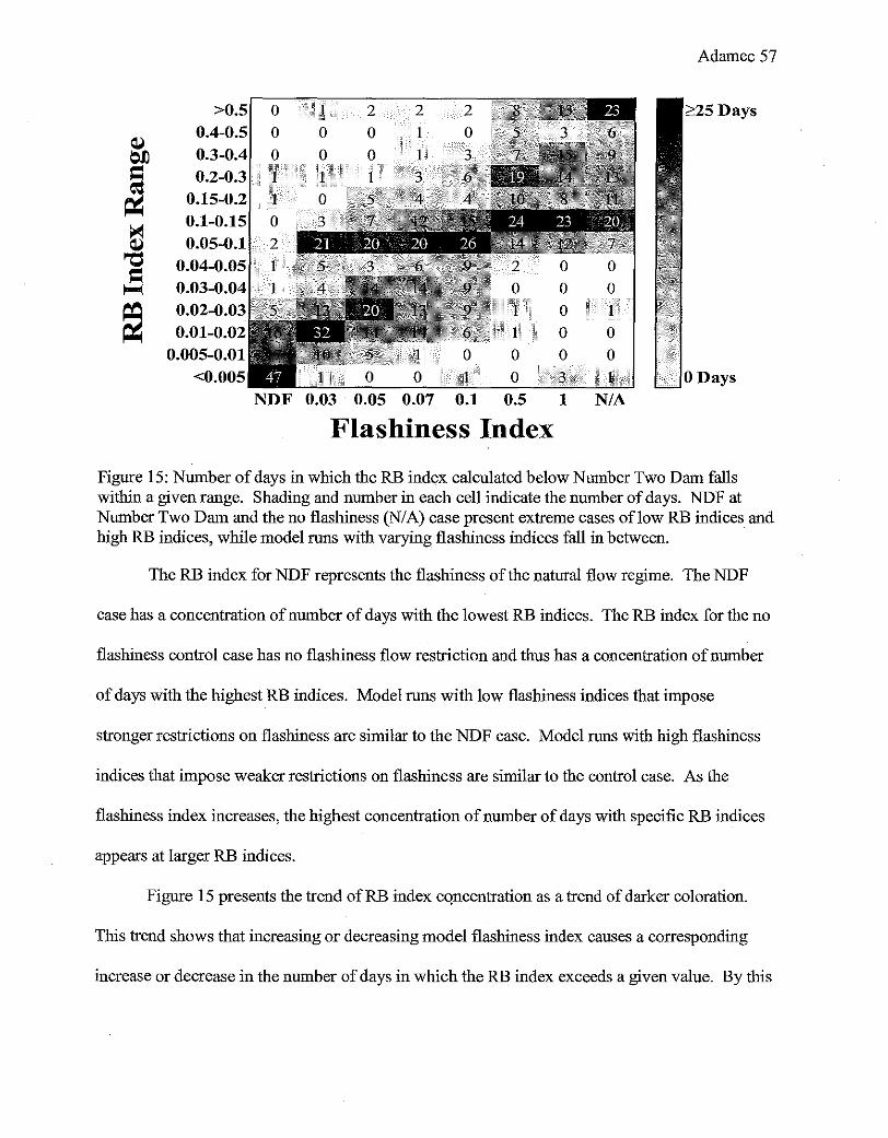
Adamec 57

>0.5 0 2 2 2 Days 0.4-0.5 0 0 0 1 0

0 0 1

1 i 0

0 1 i 0

1 0 0

0 0 0

<0.005 0 0 3 NDF 0.03 0.07 0.1 0.5 1 N/A

Flashiness Index

Figure 15: Number of days in which the RB index calculated below Number Two Dam falls within a given range. Shading and number in each cell indicate the number of days. NDF at Number Two Dam and the no flashiness (N/ A) case present extreme cases of! ow RB indices and high RB indices, while model runs with varying flashiness indices fall in between.

The RB index for NDF represents the flashiness of the natural flow regime. The NDF

case has a concentration of number of days with the lowest RB indices. The RB index for the no

flashiness control case has no flashiness flow restriction and thus has a concentration of number

of days with the highest RB indices. Model runs with low flashiness indices that impose

stronger restrictions on flashiness are similar to the NDF case. Model runs with high flashiness

indices that impose weaker restrictions on flashiness are similar to the control case. As the

flashiness index increases, the highest concentration of number of days with specific RB indices

appears at larger RB indices.

Figure 15 presents the trend of RB index cqncentration as a trend of darker coloration.

This trend shows that increasing or decreasing model flashiness index causes a corresponding

increase or decrease in the number of days in which the RB index exceeds a given value. By this

Adamec 58

mechanism, the flashiness flow is effective at controlling flashiness in the sub-daily model and

the FI may be derived from the desired number of days that exceed a given RB index.

Another way oflooking at RB index exceedance is by measuring the number of days in

which the RB index exceeds a specific reference RB index. In Figure 15, as the flashiness index

increases, the number of days in which the RB index exceeds a specific value, as measured by all

of the days in RB index ranges above that value, increases. Figure 16 presents number of days

exceeding an RB index of 0.05. The control case with no flashiness restriction exceeds aRB

index of0.05 for 89 of the 91 days of FalL Models with flashiness indices ofl and 0.5 perform

similarly. A flashiness index of0.03 only exceeds aRB index of0.05 on 26 days. A model run

with a flashiness index of 0.01 is infeasible due to limiting reservoir operating constraints.

0 0 ~

(/) &!-

>-t1l

Cl 0

0 (0 • 0.1

~

ID 0 +om .a E ~ +0.05 ::1 z ~-

+0.03

0

0.0 0.2

+0.5

0.4 0.6

Flashiness Index

+1

' ' 0.8 1.0

Figure 16: Number of days that exceed aRB index of0.05 below Number Two Dam "~

Past work by Zinnnerman et aL (2009) provides a reference for flashiness performance

based on number of days per year exceeding aRB index of 0.05. Spring and Fall are the seasons

with the most flashiness, so assuming that the number of days in Fall which exceed an RB index

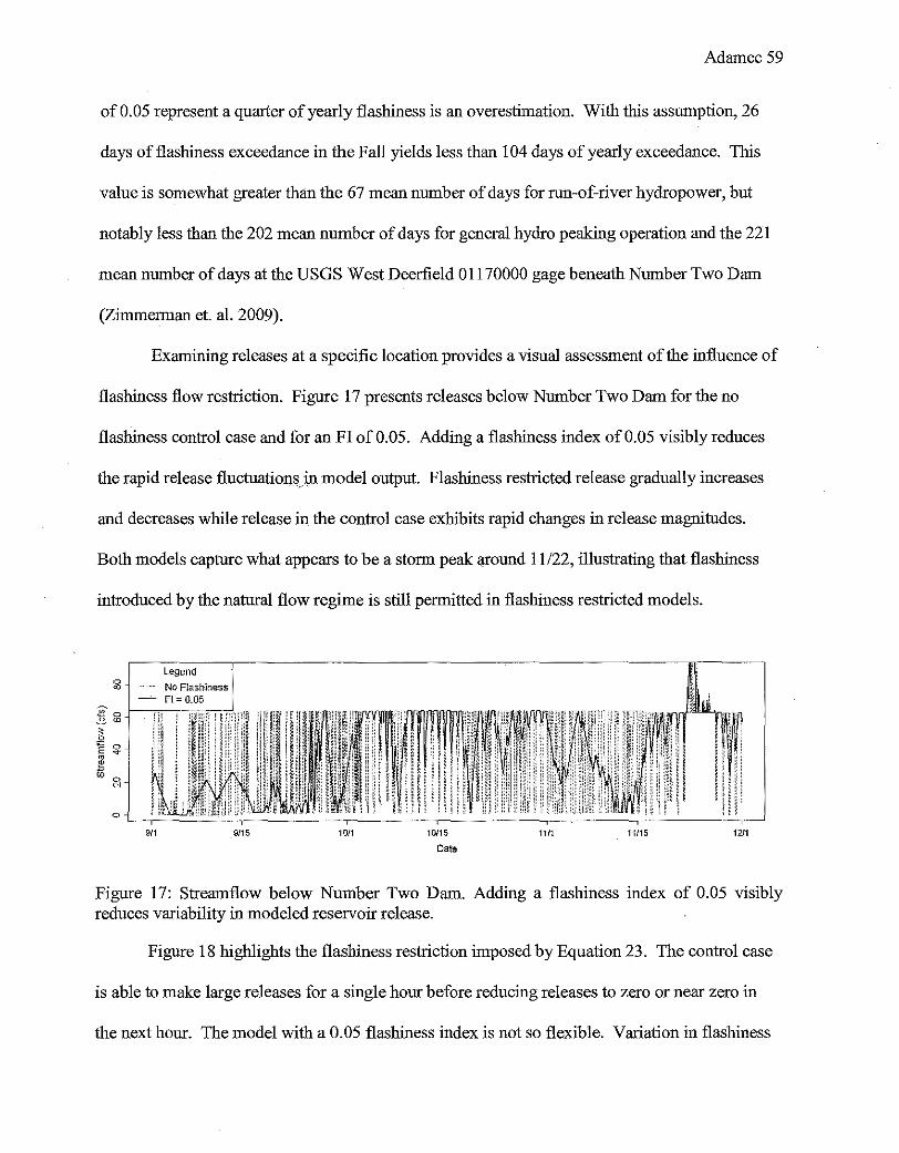
Adamec 59

of 0.05 represent a quarter of yearly flashiness is an overestimation. With this assillllption, 26

days of flashiness exceedance in the Fall yields less than 104 days of yearly exceedance. This

value is somewhat greater than the 67 mean nillllber of days for run-of-river hydropower, but

notably less than the 202 mean nillllber of days for general hydro peaking operation and the 221

mean number of days at the USGS West Deerfield 01170000 gage beneath Number Two Dam

(Zimmerman et. al. 2009).

Examining releases at a specific location provides a visual assessment of the influence of

flashiness flow restriction. Figure 17 presents releases below Nillllber Two Dam for the no

flashiness control case and for an FI of 0.05. Adding a flashiness index of 0.05 visibly reduces

the rapid release fluctuationsjn model output. Flashiness restricted release gradually increases

and decreases while release in the control case exhibits rapid changes in release magnitudes.

Both models capture what appears to be a storm peak around 11122, illustrating that flashiness

introduced by the natural flow regime is still permitted in flashiness restricted models.

0 ~

-

~ 0 ~

i5 " 0 E ~ m ~

1i5 ~

0

9/1

Legend

No Flashiness Fl = 0.05

9/15 Hl/1 10/15

Date

11/1 11115 1211

Figure 17: Streamflow below Number Two Dam. Adding a flashiness index of 0.05 visibly reduces variability in modeled reservoir release.

Figure 18 highlights the flashiness restriction imposed by Equation 23. The control case

is able to make large releases for a single hour before reducing releases to zero or near zero in

the next hour. The model with a 0.05 flashiness index is not so flexible. Variation in flashiness

Adamec60

flows due to changes in the NDF limit how much release can change for each day. Between 9/20

and 9/24, for instance, the FF tightly restricts permissible change in release and the model is

never able to make the large magnitude releases of the control case. In other cases, such as

between 9/25 and 9/27, the flashiness restricted model is able to reach the same maximum

streamflow as the control case, but must approach and depart from the large release with

incremental small hourly changes.

0 01

0

Legend

-··&··· No Flashiness

-- FI=0.05

9/21 9/22

~ n I

I!

9/23 9/24

r1jf ~ l J

r:r I·

9/25

Date

-9/26 9/27 9/28 9/29

Figure 18: Streamflow below Number Two Dam with and without flashiness control during a period of rapid change in release rates.

3.3.2 Hydropower Total model income generated by all of the modeled hydropower dams over the full

model run measures maximum possible hydropower earnings for a specified flashiness index.

Figure 19 displays total model income for models constrained by a variety of the flashiness

indices. Maximum possible income, calculated by the control model with no flashiness

Adamec 61

constraints, provides a point of reference. Even though models with Fls of 1 and 0.5 have

similar numbers of days which exceed 0.05 as the control model, visible from Figure 15, total

model income differs from maximum possible income because model changes are introduced

that decrease the occurrence of very large RB indices. The difference between maximum total

model income and total model income for flashiness index of0.03 is $104,222.

Figure 19 shows that more stringent flashiness restrictions decrease maximum possible

income from hydropower generation. The points are Pareto optimal "best" model releases and

storages for environmental needs and for hydropower, as measured by the flashiness index and

total model income. Figure 19 indicates that a large initial reduction in flashiness index from the

control case could be achieved by a relatively small reduction in maximum possible total model

income, while subsequent flashiness reduction more rapidly reduces maximum possible income.

0 0

Adamec 62

8.--------------------------------------------------------------, gij

~ 0

<f'> 0 ~ 8-<D '<T E co 0 {.) !:

<D 0 "0 0 0 8-:a;

0 (ij co 0 f- -

0 0 0 0 <.0 1'-

0.0

+0.1

+0.07 +0.05

+0.03

' 0.2

Maximum Income, No Target

+0.5

' 0.4 0.6

Flashiness Index

+1

0.8 1.0

Figure 19: Total model income for various flashiness indices. The dotted line shows the hourly model with no flashiness constraints. Total model income is the total income generated at each of the reservoirs for the year.

3.4 Conclusions

Flashiness is a characteristic of streamflow that strongly influences the environment A

typical measure of flashiness based on past literature is the Richards Baker index. The Richards

Baker index is difficult to apply directly within an optimization modeL This paper proposes a

framework for incorporating goals for Richards Baker index exceedance into an optimization

model using a flashiness flow ramping constraint calculated from a flashiness index similar to a

Richards Baker index. The flashiness flow selectively controls for flashiness due to dam

operation while permitting flashiness originating from the natural flow regime. The flashiness

flow methodology proves to be a viable means of controlling the number of days in excess of a

specified RB index.

Adamec 63

For this case, flashiness flow is incorporated in an hourly optimization model of dams on

the Deerfield River. A tradeoff between modeled hydropower income and flashiness is

generated based on modeled output. Decision makers interested in environmental concerns can

use such tradeoffs to infoi:m reservoir operations and hydropower regulation considerations.

3.5 Acknowledgements

This project was part of the Connecticut River Watershed Project, a joint partnership of

The Natore Conservancy and the U.S. Army Corps of Engineers. Funding for this project was

provided by TheN ature Conservancy.

3.6 References

Baker, D.B., et.al. (2004). A new flashiness index: characteristics and applications to

Midwestern rivers and streams. JA WRA. I 0 (2).

Bretschko, G. and Moog, 0. (1990). Downstream effects of intermittent power

generation. Wat. Sci. Tech., 22(5). 127-135.

Federal Energy Regulatory Commission (FERC), Final Environmental Impact Statement,

Deerfield River Projects. Office of Hydropower Licensing. Washington D.C. August 1996.

Harman, C. and Stewardson, M. (2005). Optimizing dam release rules to meet

environmental flow targets. River Research and Applications, 21, 113-129.

Jager, H. I. and Smith, B.T. (2008). Sustainable reservoir operation: Can we generate

hydropower and preserve ecosystem values? River. Res. Applic. 24, 340-352.

Parasiewicz, P., Schumutz, S., and Moog, 0. (1998). The effect of managed hydropower

peaking on the physical habitat, benthos and fish fauna in the River Bregenzerach in Austria.

Fisheries Management and Ecology, 5, 403-417.

Adamec64

Poff, N.L., et. AI. (1997). The natural flow regime: A paradigm for river conservation

and restoration. BioScience, 47(11 ). 769-784

Richter, B.D. and Thomas, G.A. (2007). Restoring environmental flows by modifYing

dam operations. Ecology and Society, 12(1).

Zimmerman, J.K.H., et.al. (2009). Determining the effects of dams on subdaily variation

in river flows at a whole basin scale. River. Res. Applic.

Adamec65

4 References

Adamec, K., Palmer, R.N., Polebitski, A, Ahlfeld, D., Steinschneider, S., Pitta, B., and

Brown, C. (201 0). Evaluation of climate change impacts to reservoir operations within the

Connecticut River Basin. In R.N. Palmer (Ed.) World Environmental and Water Resources

Congress 2010: Challenges of Change. Reston, VA: ASCE.

Alaya, A.B., Souissi, A, Tarhouni, J., and Ncib, K. (2003). Optimization ofNebhana

Reservoir Water Allocation by Stochastic Dynamic Programming. Water Resources

Management, 17, 259-272.

Archfield, S.A, Vogel, R.M., Steeves, P.A, Brandt, S.L., Weiskel, P.K., and Garabedian,

S.P., 2010, The Massachusetts Sustainable-Yield Estimator: A decision-support tool to assess

water availability at ungaged stream locations in Massachusetts: U.S. Geological Survey

Scientific Investigations Report 2009-5227,41 p. plus CD-ROM.

Armstrong, D.S., Parker, G.W., and Richards, T.A, 2008, Characteristics and

classification ofleast altered streamflows in Massachusetts: U.S. Geological Survey Scientific

Investigations Report 2007-5291, 113 p., plus CD-ROM.

Baker, D.B., eta!. (2004). A new flashiness index: characteristics and applications to

Midwestern rivers and streams. JA WRA. 10 (2).

Botts, AK. (1935). Water power development on the Deerfield River. Economic

Geography. 11(2), p. 148-158

Bretschko, G. and Moog, 0. (1990). Downstream effects of intermittent power

generation. Wat. Sci. Tech., 22(5). 127-135.

Adamec66

Executive Office of Environmental Affairs (EOEA). (2004). Deerfield Watershed

Assessment Report: 2004-2008. Commonwealth of Massachusetts. Retrieved from:

http://www.mass.gov/Eoeea/docs/eea/water/assess _deerfield. pdf

Federal Energy Regulatory Commission (FERC), Final Environmental Impact Statement,

Deerfield River Projects. Office of Hydropower Licensing. Washington D.C. August 1996.

Grygier, J.C., and Stedinger, J.R. (1985). Algorithms for optimizing hydropower system

operation. Water Resources Research, 21(1), 1-10.

Hanscom, M.A., Lafond, L., Lasdon, L., and.Pronovost, G. (1980). Modeling and

resolution of the medium term energy generation planning problem for a large hydro-electric

system. Management Science, 26(7), 659-668.

Harman, C. and Stewardson, M. (2005). Optimizing dam release rules to meet

environmental flow targets. River Research and Applications, 21, 113-129.

Jager, H.I. and Bevelhimer, M.S. (2007). How run-of-river operation affects hydropower

generation and value. Environmental Management, 40. 1004-1015.

Jager, H.I. and Smith, B.T. (2008). Sustainable reservoir operation: Can we generate

hydropower and preserve ecosystem values? River. Res. Applic. 24, 340-352.

Labadie, J.W. (2004). Optimal Operation ofMultireservoir Systems: State-of-the-Art

Review. Journal of Water Resources Planning and Management, 130(2), 93-111.

Loucks, D.P. and van Beek, E. (2005). Water Resources Systems Planning and

Management: An Introduction to Methods, Models, and Applications. The Netherlands:

UNESCO Publishing.

Needham, J.T., et. a!. (2000). Linear Programming for Flood Control in the Iowa and Des

Moines Rivers. Journal of Water Resources Planning and Management, 126(3), 118-127.

Adamec67

Parasiewicz, P., Schumutz, S., and Moog, 0. (1998). The effect of managed hydropower

peaking on the physical habitat, benthos and fish fauna in the River Bregenzerach in Austria.

Fisheries Management and Ecology, 5, 403-417.

Pitta, B., Palmer, R., Adamec, K., Polebitski, A., and Steinschneider, S. (2010).

Optimizing reservoir operations in the Connecticut River Basin. In R.N. Pahner (Ed.) World

Environmental and Water Resources Congress 2010: Challenges of Change. Reston, VA:

ASCE.

Poff, N.L., et. Al. (1997). The natural flow regime: A paradigm for river conservation

and restoration. BioScience, 47(11 ). 769-784

Rani, D. and Moriera, M.M. (201 0). Simulation-optimization modeling: A survey and

potential application in reservoir systems operation. Water Resour Manage, 24. 1107-1138.

Richter, B.D. and Thomas, G.A. (2007). Restoring environmental flows by modifying

dam operations. Ecology and Society, 12(1 ).

Wurbs, R.A. (1991). Optimization of Multiple-Purpose Reservoir System Operations: A

Review of Modeling and Analysis Approaches. US Army Corps of Engineers: Hydrologic

Engineering Center. Research Document No. 34.

Yeh, W.WG. (1985). Reservoir Management and Operations Models: A State-of-the-Art

Review. Water Resources Research, 21(12).

Yeh, W.WG. Becker, L., and Chu, W-S. (1979). Real-time hourly reservoir operation.

Journal of the Water Resources Planning and Management Division, 105(2), 187-203.

Zimmerman, J.K.H., et.al. (2009). Determining the effects of dams on subdaily variation

in river flows at a whole basin scale. River. Res. Applic.

Adamec68

5 Appendices

5.1 Appendix A: Dam Operation

Specifications and operating information for each dam are as follows. Unless otherwise

specified, information is derived from personal communication with TransCanada, a company

' that owns most of the Deerfield dams (TransCanada, personal communication, 2009-2011).

5.1.1 Somerset Dam The most upstream dam is Somerset Dam, located at river mile 66 on the Deerfield River.

Somerset Dam has a capacity of 57,345 acre-ft. Drainage input is approximately 30 square

miles. Somerset is owned and operated by TransCanada as a storage reservoir. Somerset

controls th!< J:llajority of the water in the Deerfield system and releases from Somerset influence

hydropower generation downstream (Botts 1935).

Somerset has a minimum release that changes annually. From May 1 to July 31, the

minimum release is 12 cfs or the inflow, but not less than 9 cfs. From August 1 to September 30,

the minimum release is 12 cfs. From October 1 to December 15, the minimum release is 30 cfs.

From December 16 to the last day of February, the minimum release is 48 cfs. From March 1 to

April 30, the minimum release is 30 cfs.

Somerset reservoir is a loon nesting area. To provide adequate habitat during the loon

nesting season, the reservoir is stabilized at a specific elevation. From May 1 to May 31, an

attempt is made to fill the reservoir to 2128.58 ft msl. If that elevation is reached, the reservoir is

stabilized at that level± 3 ft until July 31. If that elevation is not reached by June 1, the reservoir

is stabilized at the June 1 elevation ± 3 ft.

The maximum release from Somerset is the greater of312 cfs or the inflow, except

during loon season. From August 1 to November 1, the elevation of the reservoir must be

Adamec69

greater than 2120 ft msl. Outside of that period, reservoir elevation must be greater than 2107 ft

msl. The maximum operating elevation of the reservoir is 2133.58 ft msl. Between August 1

and April 30, ramping at Somerset is restricted to 100 cfs per 24 hours ramping up and 50 cfs per

24 hours ramping down.

5.1.2 Searsburg Dam Searsburg Dam is located at approximately river mile 60. Searsburg has a capacity of

600 acre-ft. The primary use of the dam is as run of river hydropower. Searsburg is owned and

operated by TransCanada. The dam diverts water from the river through a three mile penstock to

a powerhouse, returning the water just upstream of Harriman Dam (EOEA 2004). It also

releases water to the bypass reach, maintaining water in the river (EOEA 2004). Searsburg has

one generating unit. The maximum power generated by the unit is 5 MW. The power station

has a maximum flow of 345 cfs. Inputs to the reservoir include release from Somerset and

approximately 60 square miles of drainage.

Searsburg has a minimum release requirement of the minimum of 35 cfs or inflow

between June 1 and September 30 and the minimum of 55 cfS or inflow between October 1 and

May 31 in the bypass. Below the tailrace, after water used for power generation has combined

with water transmitted directly over the dam, the minimum release is 175 cfs between April20

and May 15. The Searsburg reservoir has a target operating range ofbetween 1743.66 and

1754.66 ft msl from May 1 to October 31 and between 1746.66 and 1754.66 ft msl from

November 1 to April30.

5.1.3 Harriman Dam Harriman Dam is located at river mile 48.5. Harriman has a capacity of318,000 acre-ft.

The primary use of the dam is as storage hydropower. Harriman is owned and operated by

TransCanada. It releases water either from the dam directly into the river or through an

Adamec70

excavated tunnel to a powerhouse (EOEA 2004). Harriman has three generating units with a 15

MW generating potential each for a total of 45 MW. Each unit has a limit of 600 cfs, for a total

of 1800 cfs. Inputs to the reservoir include release from Sears burg and approximately 94 square

miles of drainage.

Harriman has a minimum release requirement on flows through the bypass of 57 cfs

between July 1 and September 30 and 70 cfs between October 1 and June 30. In the spring,

Harriman has a target to fill the reservoir to the maximum elevation of 1493.66 ft msl. Between

April1 and June 15, the reservoir elevation must be stable or rising. From April1 to November

1, provided it does not interfere with the stable or rising requirement, the maximum draw down

elevation is limited to 1475 ft msl. The maximum annual drawdown elevation (for all other

times of the year) is 1440 ft msl.

5.1.4 Sherman Dam Sherman Dam is located at river mile 42 in Rowe, MA. Sherman has a capacity of3593

acre-ft. The primary use of the dam is as run of river hydropower. Sherman is owned and

operated by TransCanada. It generates water without bypassing the river (EOEA 2004).

Sherman has one 6.4 MW generating unit and a maximum generating flow of 1150 cfs. Inputs to

the reservoir include release from Harriman and approximately 50 square miles of drainage.

Sherman must allow Number Five to meet the minimum flow of73 cfs or inflow, but no

less than 57 cfs. Sherman also has a whitewater release schedule that mandates 26 weekend and

6 Friday releases. Negotiated whitewater releases include: 2 weekend days in May, 5 weekend

days and 2 Fridays in June, 6 weekend days and 2 Fridays in July, 6 weekend days and 2 Fridays

in August, 4 weekend days in September, and 2 weekend days in October, while minimizing the

number of 3 consecutive day releases. Equal number of releases should be made of 900, 1000,

and 1100 cfs. Friday releases are 4 hours starting at 11 am. Saturday releases are 5 hours

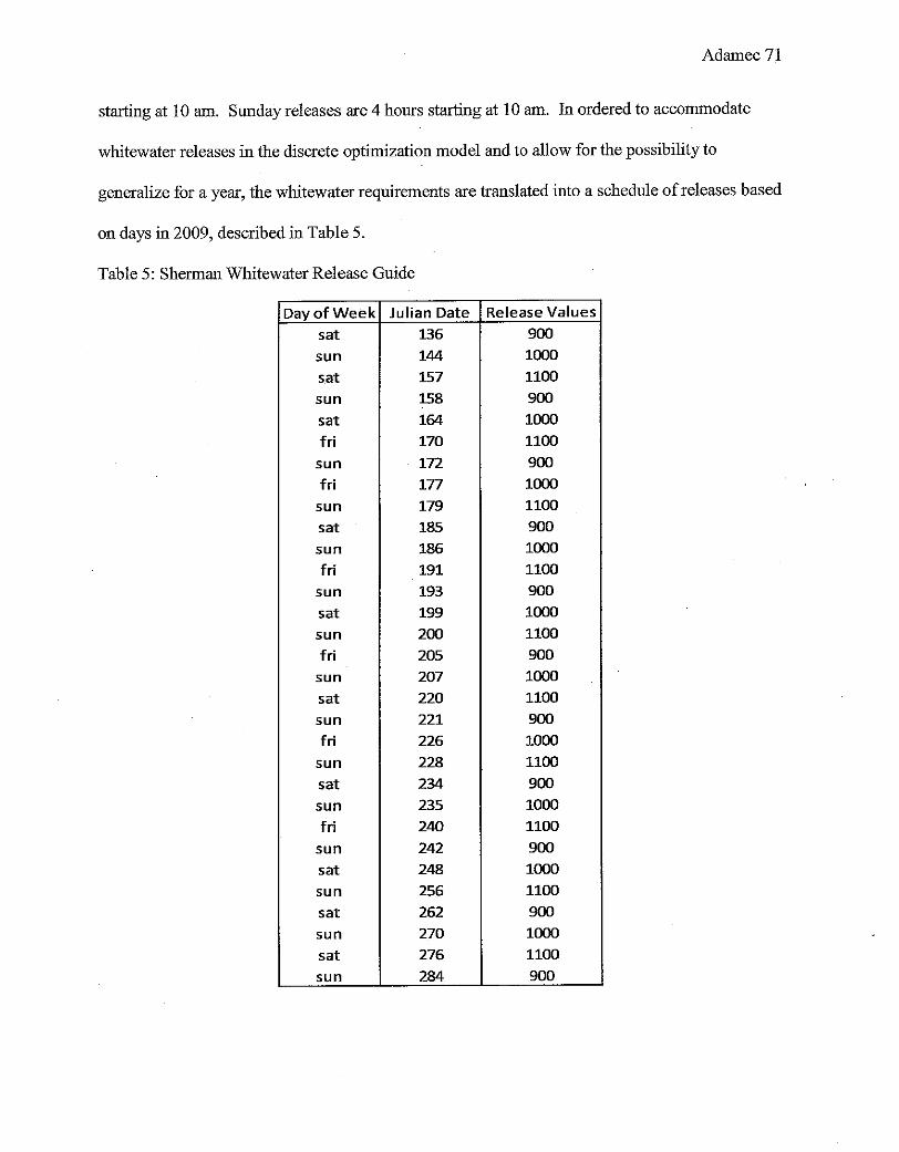
Adamec 71

starting at 10 am. Sunday releases are 4 hours starting at 10 am. In ordered to accommodate

whitewater releases in the discrete optimization model and to allow for the possibility to

generalize for a year, the whitewater requirements are translated into a schedule of releases based

on days in 2009, described in Table 5.

Table 5: Sherman Whitewater Release Guide

Day of Week Julian Date Release Values

sat 136 900 sun 144 1000

s.at 157 1100 sun 158 900

sat 164 1000 fri 170 1100

sun 172 900 fri 177 1000

sun 179 1100 sat 185 900 sun 186 1000

fri 191 1100 sun 193 900

sat 199 1000 sun 200 1100 fri 205 900

sun 207 1000

sat 220 1100 sun 221 900 fri 226 1000

sun 228 1100

sat 234 900 sun 235 1000 fri 240 1100

sun 242 900 sat 248 1000 sun 256 1100 sat 262 900 sun 270 1000 sat 276 1100 sun 284 900

Adamec72

5.1.5 Number Five Number Five is located at river mile 41.2. Number Five has a capacity of 118 acre-ft.

The primary use of the dam is as ruu of river hydropower. Number Five is owned and operated

by TransCanada. Water here is diverted about 5 miles through a penstock to a powerhouse

(EOEA 2004). Number Five has one 12 MW generating unit and a maximum generating flow of

1000 cfs. Inputs to the reservoir include release from Sherman and approximately 3 square miles

of drainage. Number Five has a minimum flow requirement of 73 cfs or inflow, but no less than

57 cfs.

5.1.6 Fife Brook/Bear Swamp Water from Number Five enters Fife Brook, located at river mile 37 in Florida, MA. Fife

Brook can pump water up to Bear Swamp Pumped Storage on Negus Mountain, described as

river mile 39. Fife Brook has a capacity of 4900 acre-ft and Bear Swamp has a capacity of 5260

acre-ft.

Together, Fife Brook and Bear Swap make up a pumped storage facility. The Bear

Swamp Pumped Storage facility is owned and operated by Brookfield Power, a subsidiary of

Brookfield Asset Management. Data for Fife Brook and Bear Swamp are derived from

Brookfield Power (Brookfield Power, personal communication, December 3, 2009). Pumped

storage works by transferring water between a reservoir at a lower elevation, in this case Fife

Brook, and a reservoir at a higher elevation, in this case Bear Swamp. Water is pumped from

Fife Brook to Bear Swamp when energy prices are low, typically early morning and late evening.

When energy prices are high, water released from Bear Swamp through turbines to Fife Brook

generates energy. Fife Brook also generates power at the dam, without bypassing the river

(EOEA 2004). Inputs to Fife brook include release from Number 5 and approximately 17 square

miles of drainage. Fife Brook must maintain a release of 125 cfs or greater.

Adamec 73

Fife Brook has one 9 MW generating unit and a maximum generating flow of 1000 cfs.

Bear Swamp has 2 units at 290 MW each, for a total of 580 MW. Generating head between Bear

Swamp and Fife Brook is 730 ft.

5.1.7 Number Four The Deerfield River flows without obstruction for about 17 miles to Number Four.

Number Four has a capacity of467 acre-ft. The primary use of the dam is as run of river

hydropower. Number Four is owned and operated by TransCanada. Water at Number Four is

diverted 1.5 miles to a powerhollSe'and re-enters the river just above Number Three (EOEA

2004). Number Four has three units at 2 MW each for a total of 6 MW. Each unit has a

maximum generating flow of 500 cfs for a total of 1500 cfs. Inputs to the reservoir include

release from Fife Brook and approximately 150 square miles of drainage.

Number Four has a minimum flow requirement of 100 cfs or inflow between October 1

and May 31 and 125 cfs or inflow between June 1 and September 30. There is also a smolt

passage flow requirement of 60 cfs from Aprill to June 15 and from September 15 to November

15.

5.1.8 Number Three Number Three is located at river mile 17 in Shelburne Falls, MA (EOEA 2004). Number

Three has a capacity of221 acre-ft. The primary use of the dam is as run of river hydropower.

Number Three is owned and operated by TransCanada Number Three diverts water 0.4 miles to

a powerhouse and re-enters the river into Gardners Falls (EOEA 2004). Number Three has three

units at 2 MW each for a total of 6 MW. Each unit has a maximum generating flow of 500 cfs

for a total of 1500 cfs. Inputs to the reservoir include release from Fife Brook and approximately

96 square miles of drainage.

Adamec 74

Number Three has a minimum flow requirement of 100 cfs or inflow. There is also a

smolt passage flow of 100 cfs from April! to June 15 and from September 15 to November 15.

5.1.9 Gardners Falls Gardners Falls is located at river mile 15.7. Gardners Falls has a capacity of510 acre-ft.

The primary use of the dam is as run of river hydropower. The Gardners Falls facility went into

operation in 1904. It was first operated by Greenfield Electric Light and Power Company,

followed by Turners Falls Power and Electric Company and Consolidated Edison, and finally by

North America Energy Alliance (NAEA) LLC. The facility diverts water for about 0.3 miles

through a powerhouse (EOEA 2004). Gardners Falls has a minimum release of 150 cfs. The

generating capacity of the dam is approximately 3.6 MW. Inputs to the reservoir include release

from Number Three and approximately 2 square miles of drainage.

5.1.10 Number Two About 2.5 miles below Gardners Falls is Number Two, located at river mile 13.2.

Number Two has a capacity of550 acre-ft. The primary use of the dam is as run of river

hydropower. Number Two is owned and operated by TransCanada. Number Two is the last

hydropower facility on the Deerfield River. Power is generated at Number Two without

bypassing the river (EOEA 2004). Number Three has three uuits at 2 MW each for a total of 6

MW. Each uuit has a maximum generating flow of 500 cfs for a total of 1500 cfs. Inputs to the

reservoir include release from Gardners Falls and approximately 3 square miles of drainage.

Following Number Two, the Deerfield River joins the Connecticut River in Greenfield, MA.

Number Two has a minimum release requirement of 200 cfs. There is also a smolt

passage flow of30 cfs from April 1 to June 15 and from September 15 to November 15.

5.2 Appendix B: Deerfield Model Base Case Equations and Variables

5.2.1 Base Case Equations N T

Adamec75

min L L ( -a1fJ1ln,t + az(fJzA~,t + f33Bh,t) + a3(f34A~,t + f3sB:f.t)) [26] n::;::lt::::l

Sn,t = Sn,t-1 + Qn,t - Rn,t [27]

sn,t=1 = Sn,max = Sn,t=T [28]

[29]

[30]

ln,t = Ct * R~,t * h.n,t * Y * 1J * \j! [31]

[32]

0 :::; R~,t :::; R~,MAX [33]

0 :::; R~,t :::; R~,MAX [34]

Sn,t - En,t = A~,t - B~,t [35]

[36]

[37]

Rn,t - Hn,t = A~,t - B:f.t [38]

Adamec 76

t2 t 4 t 2

L Rn,t-1 - j < L Rn,t ::; L Rn,t-1 + k [39]

t=tl t=t3 t=t1

5.2.2 Variable Guide n Reservoir number within the system, starting with 1 at the most upstream and

increasing for more downstream reservoirs

N Total number of modeled reservoirs

t Time step index

T Total number of time steps modeled

Sn t Storage in n at t [ cf]

Qn,t Inflow entering n during t [cf/t]

Dn,t Drainage accrued between n -1 and n during t [cfi't]

Rn t Release from n overt [ cfi't]

R;? t Release directly to the river from n over t [ cfi't]

R~ t Release for power generation from n overt, limited by bypass or turbine capacity

[ cfi't]

ln,t Income due to power generation at n overt [$]

Ct Price of energy at t, used to convert energy into income [$/MWh]

h,,t Head ofn at t, approximated as maximum dam height [ft]

!] Turbine efficiency, approximated as 0.9

y 62.4[ftlbs/s]

tji Conversion factor from ft-lbds to MWh, roughly equivalent to 1.356x10-6

J Ramping down [ cf]

Adamec 77

k Ramping up [ cf]

E Target maximum storage [ cf]

F Target minimum storage [ cf]

G Target maximum release [ cfi't]

H Target minimum release [ cfi't]

A* Value (release or storage) above the given(* = E,F,G, or H) target [ cfi't]

B* Value (release or storage) below the given(*= E,F,G, or H) target. [cfi't]

a Normalization coefficient

p Weight coefficient

Adamec 78

5.3 Appendix C: Time Step Model Changes

Specific model changes implemented to shift between one time step and the next include:

• Averaging input from hourly streamflow and energy prices to the desired time step

• Duplicating storage target variables so that storage targets remain constant for each

time step in a day

• Adjusting the factor that represents the number oftime steps per day

• Adjusting preprocessing of the Division 5 minimum target. Division 5 has a

minimum release of73 cfs or inflow, but no less than 57 cfs. The 57 cfs must be

converted into cubic feet by multiplying by the number of seconds per time step.

Storage targets and release bounds are enforced for each time step in a day. In the case of

the Deerfield, the primary storage target is on Somerset reservoir to constrain water levels within

± 3 inches during the loon nesting season. Sub-daily storage changes would not satisfY the

environmental concern, so the target is applied at each time step.

Ramping is a maximum or minimum shift in daily release. Limits on ramping are

quantified by reservoir operators in units of cfs/day or as water level shift in ftlday. Model

implementation of ramping maintains the daily restriction regardless of time step. As described

in Equation 14, the model constrains the total releases in a day as greater and less than a given

difference from the sum of releases for the prior day.

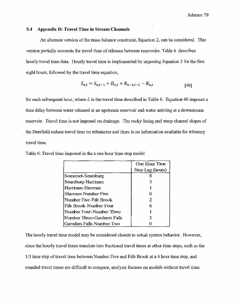
Adamec79

5.4 Appendix D: Travel Time in Stream Channels

An alternate version of the mass balance constraint, Equation 2, can be considered. This

version partially accounts for travel time of releases between reservoirs. Table 6 describes

hourly travel time data. Hourly travel time is implemented by imposing Equation 2 for the first

eight hours, followed by the travel time equation,

Sn t = Sn t-1 + Dn t + Rn-1 t-L - Rn t , J ' , ' [40]

for each subsequent hour, where L is the travel time described in Table 6. Equation 40 imposes a

time delay between water released at an upstream reservoir and water arriving at a downstream

reservoir. Travel time is not imposed on drainage. The rocky lining and steep channel slopes of

the Deerfield reduce travel time on tributaries and there is no information available for tributary

travel time.

Table 6: Travel time imposed in the a one hour time step model

One Hour Time Step Lag (hours)

Somerset-Searsbmg 8 Sears burg-Harriman 3 Harriman-Sherman 1 Sherman-Nl.llilber Five 0

Nl.llilber Five-Fire Brook 2 Fire Brook-Number Fom 6 Number F om-Number Tbree 1 Number Three-Gardners Falls 3 Garnders Falls-Number Two 0

The hourly travel time model may be considered closest to actual system behavior. However,

since the hourly travel times translate into fractional travel times at other time steps, such as the

1/3 time step of travel time between Number Five and Fife Brook at a 6 hour time step, and

rounded travel times are difficult to compare, analysis focuses on models without travel time.

Adamec80

Preliminary model results reveal a percent error of0.03 in total income variation of the hourly

models with and without travel time. Neglecting travel time is not an unreasonable assumption

as hourly models with and without travel time are similar and hourly models should exhibit the

greatest differences due to travel time spanning the greatest number of time steps.

Adamec 81

5.5 Appendix E: Expected Sub-Daily Results

Model results can be assessed after the model is verified. Allowing the model to

optimize over a shorter time step provides greater degrees of freedom. One of the advantages of

hydropower is the ability to store water when energy prices are low and release water to generate

power when energy prices are high. The daily model uses average daily energy price and inflow.

The shorter time step of sub-daily models allows the model to maximize income over the course

of the day. Because the sub-daily models have more flexibility and allow for the optimum

release selection, it is a natural, but false, hypothesis that sub-daily optimization will always

perform better than daily optimization.

It remains theoretically possible for sub-daily optimization to perform worse than daily

optimization. The averaging used to attain daily model input could be an advantage in some

cases. Table 7 describes an example based on a reservoir in the Deerfield. In this example, price

of energy and inflow range from realistic high values in the first time step to realistic lower

values in the last two time steps. As in the Deerfield models used in this analysis, the daily

model uses the average energy price and total inflow, effectively assuming an even distribution

of energy price and the inflow over the day. The 6 hour model is forced to spill in the first time

step. The daily model has no need to spill because inflow is distributed over the day, and

ultimately is able to generate a greater income.

Adamec 82

Table 7: Example of poor sub-daily performance. A 6 hour model is generates less income than a daily model because the 6 hour model is forced to spill and the daily model is not. Units of kef indicate I 000 cubic feet.

# 2 Station Storage Capacity Head Turbine Efficiency Minimum Release Turbine Capacity

Price of Energy ($/MWh) Inflow (kcJ) Storage (kcl) Power Release (kcJ) Other Release (kcJ)

Final Income($) F ina! Storage (kcl)

24000 kef 11ft

0.9 43000 kd16brs 32000 kc116brs

0-6brs 6-12brs 20 40

33000 31000 24000 24000 32000 31000

1000 0

172000 kcJ!day 128000 kcJ!day

12-18brs 18-24brs 90 90

30000 30000 24000 22000 32000 32000

0 0 6Hour

1778 20000

Daily 60

124000 24000

128000 0

Daily 1787

20000

Adamec 83

5.6 Appendix F: Sub-Daily Model Results

0 0

~ 0 ~ 0 ..., ;:; $ ., Ol 0 !::! 0

~ g 'li> ~ .,

Reservoir storages and releases are displayed below for daily and hourly model runs.

-...... ,_ ... '-"'"'_ ... --.__,- _____ ,., __ t • •

E o 0 0

(/) 0 _J--------, o Legend ~

0

Daily Model ---- 1 Hour Model


Day of Year

Figure 20: Somerset daily and hourly storage .

0 ~ 0 .1!! "" 0 ~ ., If) nl 0,1 0 (i; 0 0:: N

'li> "' ... 0,1

E 0 0 0 (/)

,..

0

' " 1•,1

' '

.. .. .. .. .. .. .. .. .. .. .. .. .. .. .. ' • •

Legend Daily Model

---- 1 Hour Model


Day of Year

Figure 21: Somerset daily and hourly release.

~

¢:!

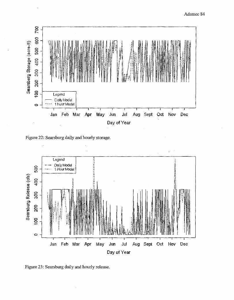
' ~ 0

"' ~ <1> 0> 1:! 0 ~

(I)

0> '-<1> .Q !!! "' <1>

(I)

0 0 ,._ 0 0

"' 0 0 t.(')

0 0 '<!"

Cl Cl <')

Cl 0 N

0 0

'"" 0

Legend Model

Model

:'

Adamec 84


Day of Year

Figure 22: Searsburg daily and hourly storage.

Cl Cl t.(')

0

Legend Daily Model 1 Hour Model

" " " " " " "


Day of Year

Figure 23: Searsburg daily and hourly release.

Adamec 85

0 0 g-tO (")

-~

':!: 0 0 .... 2-<>

"' tO _, "" <!>

Cl -"' ... 0 0 0 - 0 (/)

0 c tO ro ...... . § -~

ro 0 :I: 0

0 0

Legend tO - Daity Model 0- ·--- 1 Hour Model

I I I I I I ' I I I


Day of Year

Figure 24: Harriman daily and hourly storage.

0

' _!!

Legend


Day of Year

Figure 25: Harriman daily and hourly release.

0 0 0 ~

0 0 0 (')

0 0 0 N

0

Legend

Dait;'Model ---- 1 Hour Model

' '

Adamec 86


Day of Year

Figure 26: Sherman daily and hourly storage.

0 0 1.0 ('I

0 0

~ 0 1ft N

2:. 0 ., 0

"' 10

~ ~ a:: 0 <:: 0

"' 0 E T-

~

 ..c:

0 (f) 0 10

0

·~· I '~I j~.

' I ~ ~~· , I ~~v · :. u~

. I ' ,, .~ ! ,,

~'''!,·'' ·~· " '

Legend


11 '1 --


Day of Year

Figure 27: Sherman daily and hourly release.

0

Legend


Adamec87


Day of Year

Figure 28: Number Five daily and hourly storage.

0 0 1.0 N

~ 0 .~!! 0

0 0 N ~



"' 0

"' 0 q; 1.0

0::: ....

 0 .<:: 0 IJ.. 0 ..... ~

 ..Q

E 0 :;;;; 0 z 1.0

' '' . '

----


Jan Feb Mar APr May Jun Jul Aug Sept Oct Nov Dec

Day of Year

Figure 29: Number Five daily and hourly release.

Adamec 88

Legend Daily Model

0 ---- 1 Hour Model ~ 0

'7 0 v L() h

"' ;II ._ ' ' " (.) ' '"

"' ' ' ~ ' ' ' ' "' ' ' ' t» " ' '

" ' ' E ' ' •., ' ' ' 0 • ' ' ' ~ • / • • ' (/) ' ' ' ' ' ' ' ' .::tt. . ' ' ' ' .,

' ' ' 0 ' ' ' ' 0 i ' ' ' '- ' ' m ' ' ' ' '

~ ' ' 0 ' ' 0 ··, '. u.. 0 ' ' ' ~

'. . ' " ' 0


Day of Year

Figure 30: Fife Brook daily and hourly storage.

"' "' "' "' u; a::: .::tt. 0 0 ._ !D

~ u..

8 N .,..

0 0 <0

0 0 "<<'

0 0 N

0

Jan Feb Mar Apr May Jun

' '' '' 1~~ '' !ill '


I l;

Jul Aug Sept Oct Nov Dec

Day of Year

Figure 31: Fife Brook daily and hourly release.

0 0

"" ~

0 'If 0 4) 1.0 ,_ 0

"' 0 ~

4) 0 0> '<I'

"' 0 0 i/5 0

<') ,_

"' 0 0 1.1... 0 '- N 4) ..a E 0 :::> 0 z ~

0

Adamec 89

Legend


' ;:


Day of Year

Figure 32: Number Four daily and hourly storage.

0 0 1.0

~

"' .,..

~ 4)

"' "' 0 4) 0 n; 0 0::: ~

'-:::> 0

1.1... .... 0 ..a 0

E 1.0

:::> z

0

Legend

Daily Model -~-- 1 Hour Model


Day of Year

Figure 33: Number Four daily and hourly release.

0 ~ 1.0

'IT N ., ~ 0

"' 0 ~ N ., 0>

"' ~ 0 0 1.0 U) ~ ., :!! 0

.<::: 0 1- ~ ... G) .a E 0 ::> 1.0

z

0

Adamec90

Legend Daily Model

---- 1 Hour Model

' ' '' ''


Day of Year

Figure 34: Number Three daily and hourly storage.

0 0 0 <')

., 0 Ill 0

"' 0 ., N

"ID 0:: ., ~ ~ 0

0 iii 0 ..0

~

E 0

~

z 0 1.0

0

Legend Daily Model

---- 1 Hour Model


Day of Year

Figure 35: Number Three daily and hourly release.

~

¢:: ' <ll '-<> 0$ '-' <ll 0)! <II '-0 -(f)

.!!!. (ii lL

~ <ll <:: 'E 0$ (!)

C> C> C> ~

C> C> ro

0 C>

"' 0 0 .,.. 0 0 <'I

C>

Legend

Daily Model 1 Hour Model

Adamec 91

'

-n


Day of Year

Figure 36: Gardners Falls daily and hourly storage.

0 0 L()

~ N

./!! 0 ~

<ll <II <ll

0 -.; C> 0:: LO

.!!!. ~

(ii 0 lL C>

U> 0 ..... .., '<""""

c: 'E 0 m 0 (!) LO

C>

Legend



Day of Year

Figure 37: Gardners Falls daily and hourly release.

0 0 t-

0 ~

¢:: 0

d> <0 ,_ 0 0 ro 0 ~ 1.() Cl 0 ro 0 '-0 """ -(/)

~ ,_ 0 <1> 0 .n N ~ c

0 :::> z 0 ~

0

Adamec92

Legend

Daily Model 1 Hour Model

' '

' ' ' ' ' '' '' '' " " " ,,


Day of Year

Figure 38: Number Two daily and hourly storage.

0 0 ID N

~ 0 ./!.! 0 0 0 '-' N (J)

"' 0 ..!!! 0 <1> 1.<'.1

0::: .,..

~ 0 F- 0

0 ,_ ~ 

.n E 0 :::> z 0

1.()

Legend

DaityModel ---- 1 Hour Model


Day of Year

Figure 39: Number Two daily and hourly release.

5.7 Appendix G: LINGO Model Code for Hydropower Optimization

MODEL:

SETS: index /1. . 24/; time:

!Deerfield River Sets; !InflOWSi

Adamec93

DRF_RES_SOM_Q, DRF_RES_SBG_Q, DRF_RES_HAR_Q, DRF_RES_SHR_Q, DRF_RES_DVS_Q, DRF_RES_FBR_Q, DRF_RES_DV4_Q, DRF_RES_DV3_Q, DRF_RES_GRD_Q, DRF_RES_DV2_Q,

!Storages; DRF_RES_SOM_ST, DRF_RES_SBG_ST, DRF_RES_HAR_ST, DRF_RES_SHR_ST, DRF_RES_DVS_ST, DRF_RES_FBR_ST, DRF_RES_BSP_ST, DRF_RES_DV4_ST, DRF_RES_DV3_ST, DRF_RES_GRD_ST, DRF_RES_DV2_ST,

!Releases; DRF_RES_SOM_DR, DRF_RES_SBG_PR, DRF_RES_HAR_PR, DRF_RES_SHR_PR, DRF_RES_DVS_PR, DRF_RES_FBR_PR, DRF_RES_DV4_PR, DRF_RES_DV3_PR, DRF_RES_GRD_PR, DRF_RES_DV2_PR, DRF_RES_SBG_DR, DRF_RES_HAR_DR, DRF_RES_SHR_DR, DRF_RES_DVS_DR, DRF_RES_FBR_DR, DRF_RES_DV4_DR, DRF_RES_DV3_DR, DRF_RES_GRD_DR, DRF_RES_DV2_DR, DRF_RES_FBR_R_BSP, DRF_RES_BSP_R_FBR,

!Minimum Flows; DRF_RES_SOM_R_MIN_TARG, DRF_RES_SBG_R_MIN_TARG, DRF_RES_SBG_R_MIN_TARG2, DRF_RES_HAR_R_MIN_TARG, DRF_RES_SHR_R_MIN_TARG, DRF_RES_DVS_R_MIN_TARG, DRF_RES_FBR_R_MIN_TARG, DRF_RES_DV4_R_MIN_TARG, DRF_RES_DV3_R~IN_TARG, DRF_RES_GRD_R_MIN_TARG, DRF_RES_DV2_R_MIN_TARG,

DRF_RES_SOM_R_MIN_TARG_ABOVE, DRF_RES_SBG_R_MIN_TARG_ABOVE, DRF_RES_SBG_R_MIN_TARG2_ABOVE, DRF_RES_HAR_R_MIN_TARG_ABOVE, DRF_RES_SHR_R_MIN_TARG_ABOVE, DRF_RES_DVS_R_MIN_TARG_ABOVE, DRF_RES_FBR_R_MIN_TARG_ABOVE, DRF_RES_DV4_R_MIN_TARG_ABOVE, DRF_RES_DV3_R_MIN_TARG_ABOVE, DRF_RES_GRD_R_MIN_TARG_ABOVE, DRF_RES_DV2_R_MIN_TARG_ABOVE,

DRF_RES_SOM_R_MIN_TARG_BELOW, DRF_RES_SBG_R_MIN_TARG_BELOW, DRF_RES_SBG_R_MIN_TARG2_BELOW, DRF_RES_HAR_R_MIN_TARG_BELOW, DRF_RES_SHR_R_MIN_TARG_BELOW, DRF_RES_DVS_R_MIN_TARG_BELOW, DRF_RES_FBR_R_MIN_TARG_BELOW, DRF_RES_DV4_R_MIN_TARG_BELOW, DRF_RES_DV3_R_MIN_TARG_BELOW, DRF_RES_GRD_R_MIN_TARG_BELOW, DRF_RES_DV2_R_MIN_TARG_BELOW,

!Target Storage/Elevations; DRF_RES_SOM_ST_LOONl_ABOVE, DRF_RES_SOM_ST_LOONl_BELOW, DRF_RES_SOM_ST_LOON2_ABOVE, DRF_RES_SOM_ST_LOON2_BELOW, DRF_RES_SOM_R_RAMP_MIN, DRF_RES_SOM_R_RAMP_MAX, DRF_RES_SOM_ST_TARG_MIN, DRF_RES_SOM_ST_TARG_MAX, DRF_RES_SOM_ST_TARG_MIN_ABOVE, DRF_RES_SOM_ST_TARG_MIN_BELOW, DRF_RES_SOM_ST_TARG_MAX_ABOVE, DRF_RES_SOM_ST_TARG_MAX_BELOW,

Adamec94

DRF_RES_HAR_R_RAMP, DRF_RES_HAR_ST_TARG_MIN, DRF_RES_HAR_ST_TARG_MIN_ABOVE, DRF_RES_HAR_ST_TARG_MIN_BELOW, DRF_RES_HAR_ST_TARG_ABOVE, DRF_RES_HAR_ST_TARG_BELOW, DRF_RES_SHR_R_MIN_TARG2, DRF_RES_DV4_DR_MIN_TARG, DRF_RES_DV3_DR_MIN_TARG, DRF_RES_DV2_DR_MIN_TARG, DRF_RES_SHR_R_MIN_TARG2_ABOVE, DRF_RES_SHR_R_MIN_TARG2_BELOW, DRF_RES_DV4_DR_MIN_TARG_ABOVE, DRF_RES_DV4_DR_MIN_TARG_BELOW, DRF_RES_DV3_DR_MIN_TARG_ABOVE, DRF_RES_DV3_DR_MIN_TARG_BELOW, DRF_RES_DV2_DR_MIN_TARG_ABOVE, DRF_RES_DV2_DR_MIN_TARG_BELOW,

!Energy Generation; DRF_RES_SBG_P, DRF_RES_HAR_P, DRF_RES_SHR_P, DRF_RES_DV5_P, DRF_RES_FBR_P, DRF_RES_DV4_P, DRF_RES_DV3_P, DRF_RES_GRD_P, DRF_RES_DV2_P, DRF_RES_BSP_P,

!Energy Prices and Income; DRF_RES_SBG_INC, DRF_RES_HAR_INC, DRF_RES_SHR_INC, DRF_RES_DV5_INC, DRF_RES_FBR_INC, DRF_RES_DV4_INC, DRF_RES_DV3_INC, DRF_RES_GRD_INC, DRF_RES_DV2_INC, DRF_RES_BSP_INC, Energy_Price, Total_Power, Total_Income;

ENDSETS

DATA: !Import the following from Excel Spreadsheet;

This is all of the node inflows (Q), storages (ST), targets (TARG), and ramping constants (RAMP);

time~ @ole('\LING011\DRF-1hr-2.xlsx');

!Add scale shift; SCALE_SHIFT ~ @ole('\LING011\DRF-1hr-2.xlsx');

DRF RES SOM_ST_MAX~ 2318560200;

DRF_RES_SBG_ST_MAX~ 26136000;

DRF_RES_HAR_ST_MAX~ 13852080000; DRF_RES SHR_ST_MAX~ 156511080; DRF_RES_FBR_ST_MAX~ 213444000; DRF_RES_BSP_ST_MAX~ 229125600; DRF_RES_DV5 ST_MAX~ 5140080; DRF_RES_DV4 ST_MAX~ 20342520; DRF_RES_DV3_ST_MAX~ 9626760; DRF_RES_GRD_ST_MAX~ 44064000; DRF_RES_DV2 ST_MAX~ 23958000;

DRF_RES_SOM_ST_MIN~ 739708200; DRF_RES_SBG_ST_MIN~ 9365400; DRF_RES_HAR_ST_MIN~ 606573000; DRF_RES_SHR_ST_MIN~ 97313040; DRF_RES_FBR_ST_MIN~ 4356000; DRF_RES_BSP_ST_MIN~ 87120000; reserve, now a temp value; DRF_RES_DV5 ST_MIN~ 784080; DRF_RES_DV4 ST_MIN~ 1524600; DRF_RES_DV3 ST_MIN~ 914760;

!57345 acre-ft;

! 412 acre-ft;

!318000 acre-ft; ! 3593 acre-ft; !4900 acre-ft; !5260 acre-ft; !118 acre-ft; !467 acre-ft; !221 acre-ft; !510 acre-ft; !550 acre-ft;

!have a minimum amnt in emergency

DRF_RES_GRD_ST_MIN~ 304920; DRF_RES_DV2_ST_MIN~ 2178000;

!Inflows to Reservoirs; DRF_RES_SOM_Q @ole('\LING011\DRF-lhr-2.xlsx'); DRF_RES_SBG_Q @ole('\LING011\DRF-lhr-2.xlsx'); DRF_RES_HAR_Q @ole('\LING011\DRF-lhr-2.xlsx'); DRF_RES_SHR_Q @ole ( '\LINGOll \DRF-lhr-2 .xlsx' ).; DRF_RES_DVS_Q @ole('\LING011\DRF-lhr-2.xlsx'); DRF_RES_FBR_Q @ole('\LING011\DRF-lhr-2.xlsx'); DRF_RES_DV4_Q @ole('\LING011\DRF-lhr-2.xlsx'); DRF_RES_DV3_Q @ole('\LING011\DRF-lhr-2.xlsx'); DRF_RES_GRD_Q @ole('\LING011\DRF-lhr-2.xlsx'); DRF_RES_DV2_Q @ole('\LING011\DRF-lhr-2.xlsx');

!Energy Prices; Energy_Price ~ @ole('LING011\DRF-lhr-2.xlsx');

!Minimum Releases for Reservoirs; DRF_RES_SOM_R_MIN_TARG ~ @ole('\LING011\DRF-lhr-2.xlsx'); DRF_RES_SOM_ST_TARG_MIN ~ @ole('\LING011\DRF-lhr-2.xlsx'); DRF_RES_SOM_ST_TARG_MAX ~ @ole('\LING011\DRF-lhr-2.xlsx'); DRF_RES_SBG_R_MIN_TARG @o1e ( '\LINGOll \DRF-lhr-2 .xlsx'); DRF_RES_HAR_R_MIN_TARG ~ @ole('\LING011\DRF-lhr-2.xlsx'); DRF_RES_SHR_R_MIN_TARG ~ @ole('\LING011\DRF-lhr-2.xlsx'); DRF_RES_SHR_R_MIN_TARG2 ~ @ole('\LING011\DRF-lhr-2.xlsx'); DRF_RES_FBR_R_MIN_TARG ~ @ole('\LING011\DRF-lhr-2.xlsx'); DRF_RES_DVS_R_MIN_TARG ~ @ole('\LING011\DRF-lhr-2.xlsx'); DRF_RES_DV4_R_MIN_TARG ~ @ole('\LING011\DRF-lhr-2.xlsx'); DRF_RES_DV4_DR_MIN_TARG ~ @ole('\LING011\DRF-lhr-2.xlsx'); DRF_RES_DV3_R_MIN_TARG ~· @ole(' \LINGOll \DRF-lhr-2 .xlsx'); DRF_RES_DV3_DR_MIN_TARG ~ @ole('\LING011\DRF-lhr-2.xlsx'); DRF_RES_GRD_R_MIN_TARG ~ @ole('\LING011\DRF-lhr-2.xlsx'); DRF_RES_DV2_R_MIN_TARG ~ @ole('\LING011\DRF-lhr-2.xlsx'); DRF_RES_DV2_DR_MIN_TARG ~ @ole('\LING011\DRF-lhr-2.xlsx');

!Ramping; DRF_RES_SOM_R_RAMP_MIN ~ @ole('\LING011\DRF-lhr-2.xlsx'); DRF_RES_SOM_R_RAMP_MAX ~ @ole('\LING011\DRF-lhr-2.xlsx'); DRF_RES_HAR_R_RAMP ~ @ole('\LINGOll\DRF-lhr-2.xlsx');

!This line exports data to the excel spreadsheet; @TEXT('onehrOut04-22.txt') ~@WRITE(

Adamec95

'DRF_RES_SOM_ST 'DRF_RES_SBG_ST 'DRF_RES_HAR_ST 'DRF_RES_SHR_ST 'DRF_RES_FBR_ST 'DRF_RES_BSP_ST 'DRF_RES_GRD_ST 'DRF_RES_SOM_DR 'DRF_RES_SBG_PR 'DRF_RES_FBR_PR 'DRF_RES_GRD_PR 'DRF_RES_SBG_DR 'DRF_RES_FBR_DR 'DRF_RES_GRD_DR 'DRF_RES_SBG_INC ', ', 'DRF_RES_FBR_INC 'DRF_RES_GRD_INC

'DRF_RES_DVS ST 'DRF_RES_DV2_ST

'DRF_RES_DV4_ST 'DRF_RES_DV3_ST

'DRF _RES_FBR_R_BSP 'DRF _RES_BSP_R_FBR ', 'DRF_RES_HAR_PR 'DRF_RES_SHR_PR 'DRF_RES_DVS PR 'DRF_RES_DV4_PR 'DRF_RES_DV3_PR 'DRF_RES_DV2 PR 'DRF_RES_HAR_DR 'DRF_RES_DV4_DR 'DRF_RES_DV2_DR

'DRF_RES_SHR_DR 'DRF_RES_DV3_DR

'DRF_RES_DV5_DR

'Total_Income ', 'Total_Power ', 'DRF_RES_HAR_INC ', ', 'DRF_RES_DV4_INC 'DRF_RES_DV2 INC

'DRF_RES_SHR_INC ', ', 'DRF_RES_DV3_INC 'DRF_RES_BSP_INC

'DRF_RES_DVS_INC

'DRF_RES_SBG_P 'DRF_RES~FBR_P

'DRF_RES_DV2_P @NEWLINE(1));

'DRF_RES_HAR_P 'DRF_RES_DV4_P 'DRF_RES_BSP_P

'DRF_RES_SHR_P 'DRF_RES_DV3_P

'DRF_RES_DV5_P 'DRF_RES_GRD_P

Adrunec96

@TEXT('onehr0ut04-22.txt') = @WRITEFOR(time(I): @FORMAT(DRF_RES_SOM_ST(I), '15£'),' @FORMAT(DRF_RES_SBG_ST(I), '15£'),' @FORMAT(DRF_RES_HAR_ST(I), '15£'),' @FORMAT(DRF_RES_SHR_ST(I), '15£'),' @FORMAT(DRF_RES_FBR_ST(I), '15f'),' @FORMAT(DRF_RES_BSP_ST(I), '15£'),' @FORMAT(DRF_RES_DV5_ST(I), '15£'),' @FORMAT(DRF_RES_DV4_ST(I), '15£'),' @FORMAT(DRF_RES_DV3_ST(I), '15£'),' @FORMAT(DRF_RES_GRD_ST(I), '15£'),' @FORMAT(DRF_RES_DV2_ST(I), '15£'),' @FORMAT(DRF_RES_SOM_DR(I), '15f'),' @FORMAT(DRF_RES_FBR_R_BSP(I), '15f'),' ', @FORMAT(DRF_RES_BSP_R_FBR(I), '15£'),' ', @FORMAT(DRF_RES_SBG_PR(I), '15£'),' @FORMAT(DRF_RES_HAR_PR(I), '15£'),' @FORMAT(DRF_RES_SHR_PR(I), '15f'),' @FORMAT(DRF_RES_DV5_PR(I), '15£'),' @FORMAT(DRF_RES_FBR_PR(I), '15£'),' @FORMAT(DRF_RES_DV4_PR(I), '15£'),' @FORMAT(DRF_RES_DV3_PR(I), '15£'),' @FORMAT(DRF_RES_GRD_PR(I), '15£'),' @FORMAT(DRF_RES_SBG_DR(I), '15f'),' @FORMAT(DRF_RES_SHR_DR(I), '15£'),' @FORMAT(DRF_RES_FBR_DR(I), '15f'),' @FORMAT(DRF_RES_DV3_DR(I), '15£'),' @FORMAT(DRF_RES_GRD_DR(I), '15£'),' @FORMAT(Total_Income(I), '15f'),' ', @FORMAT(DRF_RES_SBG_INC(I), '15£'),' @FORMAT(DRF_RES_SHR_INC(I), '15£'),' @FORMAT(DRF_RES_FBR_INC(I), '15f'),' @FORMAT(DRF_RES_DV3_INC(I), '15£'),' @FORMAT(DRF_RES_DV2_INC(I), '15f'),' @FORMAT(DRF_RES_SBG_P(I), '15£'),' @FORMAT(DRF_RES_SHR_P(I), '15f'),' @FORMAT(DRF_RES_FBR_P(I), '15£'),' @FORMAT(DRF_RES_DV3_P(I), '15f'),' @F0RMAT(DRF_RES_DV2_P(I), '15£'),' @NEWLINE(1));

END DATA

!---Objective Function---;

@FORMAT(DRF_RES_DV2_PR(I), '15£'),' @FORMAT(DRF_RES_HAR_DR(I), '15£'),' @FORMAT(DRF_RES_DV5_DR(I), '15£'),' @FORMAT(DRF_RES_DV4_DR(I), '15£'),'

@FORMAT(DRF_RES_DV2_DR(I), '15£'),' @FORMAT(Total_Power(I), '15f'),' ',

@FORMAT(DRF_RES_HAR_INC(I), '15£'),' @FORMAT(DRF_RES_DV5_INC(I), '15£'),' @FORMAT(DRF_RES_DV4_INC(I), '15f'),' @FORMAT(DRF_RES_GRD_INC(I), '15£'),' @FORMAT(DRF_RES_BSP_INC(I), '15f'),'

@FORMAT(DRF_RES_HAR_P(I), '15f'),' @FORMAT(DRF_RES_DV5_P(I), '15f'),' @FORMAT(DRF_RES_DV4_P(I), '15f'),' @FORMAT(DRF_RES_GRD_P(I), '15f'),' @FORMAT(DRF_RES_BSP_P(I), '15f'),'

!Minimizing deviations from storage, release, and eco-node release targets;

[OBJECTIVE] MIN = -(10'10)*@SUM(time(I): (1/(1096117401600*81*SCALE_SHIFT))*Total_Income(I))

!Total Income; +@SUM(time(I): (1/(DRF_RES_SOM_ST_MAX))*DRF_RES_SOM_ST_TARG_MIN_BELOW(I))

!Somerset minimum storage;

+(1/DRF_RES_SOM_ST_MAX)*@SUM(time(I) I I #GE# 121*SCALE_SHIFT #AND# I #LE# 151*SCALE_SHIFT: DRF_RES_SOM_ST_LOON1_ABOVE(I) + DRF_RES_SOM_ST_LOON1_BELOW(I)) !DRF_RES_SOM_ST_LOONDELTA_1, Somerset storage stabilization; +(1/DRF_RES_SOM_ST_MAX)*@SUM(time(I) I I #GE# 151*SCALE_SHIFT #AND# I #LE# 212*SCALE_SHIFT: DRF_RES_SOM_ST_LOON2_ABOVE(I) + DRF_RES_SOM_ST_LOON2_BELOW(I)) !DRF_RES_SOM_ST_LOONDELTA_2, Somerset storage stabilization;

Adamec97

+@SUM(time(I}: (l/(SCALE_SHIFT*(29808000+8640000000}))*DRF_RES_SBG_R_MIN_TARG_BELOW(I))

!SearsbUrg; +@SUM(time(I): (l/(SCALE_SHIFT*(29808000+8640000000}))*DRF_RES_SBG_R_MIN_TARG2_BELOW(I))

!Searsburg; +@SUM(time(I): (l/(SCALE_SHIFT*(l55520000+8640000000)))*DRF_RES_HAR_R_MIN_TARG_BELOW(I))

!Harriman; +@SUM(time(I): (l/(SCALE_SHIFT*(99360000+8640000000}))*DRF_RES_SHR_R_MIN_TARG_BELOW(I))

!Sherma~ min flow; +@SUM(time(I}: (l/(SCALE_SHIFT*(99360000+8640000000})}*DRF_RES_SHR_R_MIN_TARG2_BELOW(I))

!Sherman whitewater; +@SUM(time(I): (l/(SCALE_SHIFT*(l29600000+8640000000)))*DRF_RES_DVS_R_MIN_TARG_BELOW(I)}

!Diversion 5; . +@SUM( time (I) :

(l/(SCALE_SHIFT*(l29600000+8640000000)))*DRF_RES_DV4_R_MIN_TARG_BELOW(I)) !Diversion 4;

+5000*@SUM(time(I): (1/(SCALE_SHIFT*(129600000+8640000000)))*DRF_RES_DV4_DR_MIN_TARG_BELOW(I))

!Diversion 4 smolt; +@SUM(time(I): (l/(SCALE_SHIFT*(l29600000+8640000000)))*DRF_RES_DV3_R_MIN_TARG_BELOW(I))

JDiversion 3; +SOOO*@SUM(time(I): (l/(SCALE_SHIFT*(l29600000+8640000000}))*DRF_RES_DV3_DR_MIN_TARG_BELOW(I))

!Diversion 3 smolt; +@SUM(time(I): (1/(SCALE_SHIFT*(129600000+8640000000)}}*DRF_RES_GRD_R_MIN_TARG_BELOW(I))

!Gardner Falls; +@SUM(time(I): (l/(SCALE_SHIFT*(l29600000+8640000000}))*DRF_RES_DV2_R_MIN_TARG_BELOW(I))

!Diversion 2; +SOOO*@SUM(time(I): (l/(SCALE_SHIFT*(129600000+8640000000})}*DRF_RES_DV2_DR~IN_TARG_BELOW(I))

!Diversion 2 smolt;

!---CONTSTRAINTS ~~D TARGETS---;

!Initial Storages; @FOR (time(I) I I #EQ# 1:

[SOM_ST_l] DRF_RES_SOM_ST(I) = DRF_RES_SOM_ST_MAX + DRF_RES_SOM_Q(I) - DRF_RES_SOM_DR(I);

[SBG_ST_l] DRF_RES_SBG_ST(I) = DRF_RES_SBG_ST_MAX + DRF_RES_SBG_Q(I) - DRF_RES_SBG_PR(I) - DRF_RES_SBG_DR(I) + DRF_RES_SOM_DR(I);

[HAR_ST_l] DRF_RES_HAR_ST(I) = DRF_RES_HAR_ST_MAX + DRF_RES_HAR_Q(I) - DRF_RES_HAR_PR(I) -·DRF_RES_HAR_DR(I) + DRF_RES_SBG_PR(I) + DRF_RES_SBG_DR(I);

[SHR_ST_l] DRF_RES_SHR_ST(I) = DRF_RES_SHR_ST_MAX + DRF_RES_SHR_Q(I) - DRF_RES_SHR_PR(I) - DRF_RES_SHR_DR(I) + DRF_RES_HAR_PR(I) + DRF_RES_HAR_DR(I);

Adamec98

[DV5_ST_1] DRF_RES_DVS_ST(I) = DRF_RES_DVS_ST_MAX + DRF_RES_DVS_Q(I) - DRF_RES_DVS_PR(I) - DRF_RES_DVS_DR(I) + DRF_RES_SHR_PR(I) + DRF_RES_SHR_DR(I);

[FBR_ST_1] DRF_RES_FBR_ST(I) = DRF_RES_FBR_ST_MAX + DRF_RES_FBR_Q(I) - DRF_RES_FBR_PR(I) - DRF_RES_FBR_DR(I) + DRF_RES_DVS_PR(I) + DRF_RES_DV5_DR(I) - DRF_RES_FBR_R_BSP(I) + DRF_RES_BSP_R_FBR(I);

[BSP_ST_1] DRF_RES_BSP_ST(I) = DRF_RES_BSP_ST_MAX + DRF_RES_FBR_R_BSP(I) - DRF_RES_BSP_R_FBR(I);

[DV4_ST_1] DRF_RES_DV4_ST(I) = DRF_RES_DV4_ST_MAX + DRF_RES_DV4_Q(I) - DRF_RES_DV4_PR(I) - DRF_RES_DV4_DR(I) + DRF_RES_FBR_PR(I) + DRF_RES_FBR_DR(I);

[DV3_ST_1] DRF_RES_DV3_ST(I) = DRF_RES_DV3_ST_MAX + DRF_RES_DV3_Q(I) - DRF_RES_DV3_PR(I) - DRF_RES_DV3_DR(I) + DRF_RES_DV4_PR(I) + DRF_RES_DV4_DR(I);

[GRD_ST_1] DRF_RES_GRD_ST(I) = DRF_RES_GRD_ST_MAX + DRF_RES_GRD_Q(I) - DRF_RES_GRD_PR(I) - DRF_RES_GRD_DR(I) + DRF_RES_DV3_PR(I) + DRF_RES_DV3_DR(I);

[DV2_ST_1] DRF_RES_DV2_ST(I) = DRF_RES_DV2_ST_MAX + DRF_RES_DV2_Q(I) - DRF_RES_DV2_PR(I) - DRF_RES_DV2_DR(I) + DRF_RES_GRD_PR(I) + DRF_RES_GRD_DR(I) ) ;

!Storages; @FOR (time(I) I I #GE# 2:

[SOM_ST] DRF_RES_SOM_ST(I) DRF_RES_SOM_ST(I-1) + DRF_RES_SOM_Q(I) -DRF_RES_SOM_DR(I);

[SBG_ST] DRF_RES_SBG_ST(I) DRF_RES_SBG_ST(I-1) + DRF_RES_SBG_Q(I) -DRF_RES_SBG_PR(I) - DRF_RES_SBG_DR(I) + DRF_RES_SOM_DR(I);

[HAR_ST] DRF_RES_HAR_ST(I) = DRF_RES_HAR_ST(I-1) + DRF_RES_HAR_Q(I) -DRF_RES_HAR_PR(I) - DRF_RES_HAR_DR(I) + DRF_RES_SBG_PR(I) + DRF_RES_SBG_DR(I);

[SHR_ST] DRF_RES_SHR_ST(I) = DRF_RES_SHR_ST(I-1) + DRF_RES_SHR_Q(I) -DRF_RES_SHR_PR(I) - DRF_RES_SHR_DR(I) + DRF_RES_HAR_PR(I) + DRF_RES_HAR_DR(I);

[DVS_ST] DRF_RES_DVS_ST(I) = DRF_RES_DVS_ST(I-1) + DRF_RES_DV5_Q(I) -DRF_RES_DVS_PR(I) - DRF_RES_DV5_DR(I) + DRF_RES_SHR_PR(I) + DRF_RES_SHR_DR(I);

[FBR_ST] DRF_RES_FBR_ST(I) = DRF_RES_FBR_ST(I-1) + DRF_RES_FBR_Q(I) -DRF_RES_FBR_PR(I) - DRF_RES_FBR_DR(I) + DRF_RES_DV5_PR(I) + DRF_RES_DVS_DR(I) - DRF_RES_FBR_R_BSP(I) + DRF_RES_BSP_R_FBR(I);

[BSP_ST] DRF_RES_BSP_ST(I) DRF_RES_BSP_ST(I-1) + DRF_RES_FBR_R_BSP(I) - DRF_RES_BSP_R_FBR(I);

[DV4_ST] DRF_RES_DV4_ST(I) DRF_RES_DV4_ST(I-1) + DRF_RES_DV4_Q(I) -DRF_RES_DV4_PR(I) - DRF_RES_DV4_DR(I) + DRF_RES_FBR_PR(I) + DRF_RES_FBR_DR(I);

[DV3_ST] DRF_RES_DV3_ST(I) = DRF_RES_DV3_ST(I-1) + DRF_RES_DV3_Q(I) -DRF_RES_DV3_PR(I) - DRF_RES_DV3_DR(I) + DRF_RES_DV4_PR(I) + DRF_RES_DV4_DR(I);

[GRD_ST] DRF_RES_GRD_ST(I) = DRF_RES_GRD_ST(I-1) + DRF_RES_GRD_Q(I) -DRF_RES_GRD_PR(I) - DRF_RES_GRD_DR(I) + DRF_RES_DV3_PR(I) + DRF_RES_DV3_DR(I);

[DV2_ST] DRF_RES_DV2_ST(I) = DRF_RES_DV2_ST(I-1) + DRF_RES_DV2_Q(I) -DRF_RES_DV2_PR(I) - DRF_RES_DV2_DR(I) + DRF_RES_GRD_PR(I) + DRF_RES_GRD_DR(I) ) ;

!Energy Calculations;

@FOR(time(I): [SBG_P] DRF_RES_SBG_P(I) = DRF_RES_SBG_PR(I)*8*0.9*62.4*(1.356/1000000)*(1/3600);

[HAR_P] DRF_RES_HAR_P(I) = DRF_RES_HAR_PR(I)*57.6*0.9*62.4*(1.356/1000000)*(1/3600);

[SHR_P] DRF_RES_SHR_P(I) = DRF_RES_SHR_PR(I)*ll.6*0.9*62.4*(1.356/1000000)*(1/3600);

[DV5_P] DRF_RES_DV5_P(I) = DRF_RES_DV5_PR(I)*l0*0.9*62.4*(1.356/1000000)*(1/3600);

[FBR_P] DRF_RES_FBR_P(I) = DRF _RES_FBR_PR (I) *40*0. 9*62. 4 * (1. 356!1000000 ).* (1/3600);

[DV4_P] DRF_RES_DV4_P(I) = DRF_RES_DV4_PR(I)*5*0.9*62.4*(1.356/1000000)*(1/3600);

[DV3_P] DRF_RES_DV3_P(I) = DRF_RES_DV3_PR(I)*3*0.9*62.4*(1.356/1000000)*(1/3600);

[GRD_P] DRF_RES_GRD_P(I) = DRF_RES_GRD_PR(I)*37*0.9*62.4*(1.356/1000000)*(1/3600);

[DV2_P] DRF_RES_DV2_P(I) = DRF_RES_DV2_PR(I)*l1*0.9*62.4*(1.356/1000000)*(1/3600);

[BSP_P] DRF_RES_BSP_P(I) = DRF_RES_BSP_R_FBR(I)*730*0.9*62.4*(1.356/1000000)*(1/3600) -DRF_RES_FBR_R_BSP(I)*730*0.9*62.4*(1.356/1000000)*(1/3600);

Adamec99

[TOT_P] Total_Power(I) = DRF_RES_SBG_P(I) + DRF_RES_HAR_P(I) + DRF_RES_SHR_P(I) + DRF_RES~DV5_P(I) + DRF_RES_FBR_P(I) + DRF_RES_DV4_P(I) + DRF_RES_DV3_P(I) + DRF_RES_GRD_P(I) + DRF_RES_DV2_P(I) + DRF_RES_BSP_P(I); ) ;

!Income Calculations; @FOR(time(I): [SBG_INC] DRF_RES_SBG_INC(I) = DRF_RES_SBG_P(I)*Energy_Price(I);

) ;

[HAR_INC] DRF_RES_HAR_INC(I) DRF_RES_HAR_P(I)*Energy_Price(I); [SHR_INC] DRF_RES_SHR_INC(I) DRF_RES_SHR_P(I)*Energy_Price(I); [DVS_INC] DRF_RES_DVS_INC(I) DRF_RES_DVS_P(I)*Energy_Price(I); [FBR_INC] DRF_RES_FBR_INC(I) DRF_RES_FBR_P(I)*Energy_Price(I); [DV4_INC] DRF_RES_DV4_INC(I) DRF_RES_DV4_P(I)*Energy_Price(I); [DV3_INC] DRF_RES_DV3_INC(I) DRF_RES_DV3_P(I)*Energy_Price(I); [GRD_INC] DRF_RES_GRD_INC(I) DRF_RES_GRD_P(I)*Energy_Price(I); [DV2_INC] DRF_RES_DV2_INC(I) DRF_RES_DV2_P(I)*Energy_Price(I); [BSP_INC] DRF_RES_BSP_INC(I) DRF_RES_BSP_P(I)*Energy_Price(I); [TOT_INC] Total_Income(I) = Total_Power(I)*Energy_Price(I);

!Storage Limits; @FOR(time: [SOM_ST_LIM] @BND(DRF_RES_SOM_ST_MIN,DRF_RES_SOM_ST,DRF_RES_SOM_ST_MAX)); @FOR(time: [SBG_ST_LIM] @BND(DRF_RES_SBG_ST_MIN,DRF_RES_SBG_ST,DRF_RES_SBG_ST_MAX)); @FOR(time: [HAR_ST_LIM] @BND(DRF_RES_HAR_ST_MIN,DRF_RES_HAR_ST,DRF_RES_BAR_ST_MAX)); @FOR(time: [SHR_ST_LIM] @BND(DRF_RES_SHR_ST_MIN,DRF_RES_SHR_ST,DRF_RES_SHR_ST_MAX)); @FOR(time: [FBR_ST_LIM] @BND(DRF_RES_FBR_ST_MIN,DRF_RES_FBR_ST,DRF_RES_FBR_ST_MAX)); @FOR(time: [BSP_ST_LIM] @BND(DRF_RES_BSP_ST_MIN,DRF_RES_BSP_ST,DRF_RES_BSP_ST_MAX)); @FOR(time: [DV5_ST_LIM] @BND(DRF_RES_DV5_ST_MIN,DRF_RES_DV5_ST,DRF_RES_DV5_ST_MAX));

@FOR(time: [DV4_ST_LIM] @BND(DRF_RES_DV4_ST_MIN,DRF_RES_DV4_ST,DRF_RES_DV4_ST_MAX)); @FOR(time: [DV3_ST_LIM] @BND(DRF_RES_DV3_ST_MIN,DRF_RES_DV3_ST,DRF_RES_DV3_ST_MAX)); @FOR(time: [GRD_ST_LIM] @BND(DRF_RES_GRD_ST_MIN,DRF_RES_GRD_ST,DRF_RES_GRD_ST_MAX)); @FOR(time: [DV2_ST_LIM] @BND(DRF_RES_DV2_ST_MIN,DRF_RES_DV2_ST,DRF_RES_DV2_ST_MAX));

!Storage: STend = STstart; [SOM_ST_END] DRF_RES_SOM_ST_MAX [SBG_ST_END] DRF_RES_SBG_ST_MAX [HAR_ST_END] DRF_RES_HAR_ST_MAX [SHR_ST_END] DRF_RES_SHR_ST_MAX [DV5_ST_END] DRF_RES_DV5_ST_MAX [FBR_ST_END] DRF_RES_FBR_ST_MAX [BSP_ST_END] DRF_RES_BSP_ST_MAX [DV4_ST_END] DRF_RES_DV4_ST_MAX [DV3_ST_END] DRF_RES_DV3_ST_MAX [GRD_ST_END] DRF_RES_GRD_ST_MAX [DV2_ST_END] DRF_RES_DV2_ST_MAX

!Release Limits; @FOR(time(I): [SOM_DR_LIM]

DRF_RES_SOM_ST(@SIZE(time)); DRF_RES_SBG_ST(@SIZE(time)); DRF_RES_HAR_ST(@SIZE(time)); DRF_RES_SHR_ST(@SIZE(time)); DRF_RES_DV5_ST(@SIZE(time)); DRF_RES_FBR_ST(@SIZE(time)); DRF_RES_BSP_ST(@SIZE(time)); DRF_RES_DV4_ST(@SIZE(time)); DRF_RES_DV3_ST(@SIZE(time)); DRF_RES_GRD_ST(@SIZE(time)); DRF_RES_DV2_ST(@SIZE(time));

@BND(O,DRF_RES_SOM_DR, (l/SCALE_SHIFT)*8640000000)); @FOR(time(I): [SBG_DR_LIM] @BND(O,DRF_RES_SBG_DR, (l/SCALE_SHIFT)*8640000000)); @FOR(time(I): [HAR_DR_LIM] @BND(O,DRF_RES_HAR_DR, (l/SCALE_SHIFT)*8640000000)); @FOR(time(I): [SHR_DR_LIM] @BND(O,DRF_RES_SHR_DR, (1/SCALE_SHIFT)*8640000000)); @FOR(time(I): [DV5_DR_LIM] @BND(O,DRF_RES_DV5_DR, (1/SCALE_SHIFT)*8640000000)); @FOR(time(I): [FBR_DR_LIM] @BND(O,DRF_RES_FBR_DR, (l/SCALE_SHIFT)*8640000000)); @FOR(time(I): [DV4_DR_LIM] @BND(O,DRF_RES_DV4_DR, (l/SCALE_SHIFT)*8640000000)); @FOR (time (I) : [DV3_DR_LIM] @BND(O,DRF_RES_DV3_DR, (l/SCALE_SHIFT)*8640000000)); @FOR(time(I): [GRD_DR_LIM] @BND(O,DRF_RES_GRD_DR, (1/SCALE_SHIFT)*8640000000)); @FOR(time(I): [DV2_DR_LIM] @BND(O,DRF_RES_DV2_DR, (1/SCALE_SHIFT)*8640000000));

@FOR(time(I): [FBR_R_BSP_LIM] @BND(O,DRF_RES_FBR_R_BSP, (1/SCALE_SHIFT)*382752000)); @FOR(time(I): [BSP_R_FBR_LIM] @BND(O,DRF_RES_BSP_R_FBR, (1/SCALE_SHIFT)*382752000));

Adamec 100

@FOR(time(I): [SBG_PR_LIM] @BND(O,DRF_RES_SBG_PR, (l/SCALE_SHIFT)*29808000)); @FOR(time(I): [HAR_PR_LIM] @BND(O,DRF_RES_HAR~PR, (l/SCALE_SHIFT)*155520000)); @FOR(time(I): [SHR_PR_LIM] @BND(O,DRF_RES_SHR_PR, (1/SCALE_SHIFT)*99360000)); @FOR(time(I): [DV5_PR_LIM] @BND(O,DRF_RES_DV5_PR, (1/SCALE_SHIFT) *86400000)); @FOR(time(I): [FBR_PR_LIM] @BND(O,DRF_RES_FBR_PR, (1/SCALE_SHIFT)*86400000)); @FOR(time(I): [DV4_PR_LIM] @BND(0,DRF_RES_DV4_PR, (l/SCALE_SHIFT)*129600000)); @FOR(time(I): [DV3_PR_LIM] @BND(O,DRF_RES_DV3_PR, (1/SCALE_SHIFT)*l29600000)); @FOR(time(I): [GRD_PR_LIM] @BND(O,DRF_RES_GRD_PR, (l/SCALE_SHIFT)*l29600000));

Adamec 101

@FOR(time(I): [DV2_PR_LIM] @BND(O,DRF_RES_DV2_PR, (l/SCALE_SHIFT)*l29600000));

!Ramping; !Ramping is per day!!!; @FOR(time(I) I @WRAP(I,SCALE_SHIFT)#EQ#SCALE_SHIFT #AND# I#LT#@SIZE(time) #AND# I#GT#SCALE_SHIFT: [SOM_RMP_UP] DRF_RES_SOM_DR(I) + @SUM(index(J) !J#LT#SCALE_SHIFT: DRF_RES_SOM_DR(I+J)) < DRF_RES_SOM_DR(I-SCALE_SHIFT) + @SUM(index(J) !J#LT#SCALE_SHIFT: DRF_RES_SOM_DR(I-SCALE_SHIFT+J)) + DRF_RES_SOM_R_RAMP_MAX; !100*86400; !august 1 to april 30 (213-120), upramp 100cfs/24hrs, downramp 50cfs/24hrs; [SOM~RMP_DN] DRF_RES_SOM_DR(I) + @SUM(index(J) !J#LT#SCALE_SHIFT:

DRF_RES_SOM_DR(I+J)) > DRF_RES_SOM_DR(I-SCALE_SHIFT) + @SUM(index(J) !J#LT#SCALE_SHIFT: DRF_RES_SOM_DR(I-SCALE_SHIFT+J)) DRF_RES_SOM_R_RAMP_MIN; !50*86400; [SBG_RMP_UP] DRF_RES_SBG_PR(I) + DRF_RES_SBG_DR(I) + @SUM(index(J) !J#LT#SCALE_SHIFT: DRF_RES_SBG_PR(I+J) + DRF_RES_SBG_DR(I+J)) < DRF_RES_SBG_PR(I-SCALE_SHIFT) + DRF_RES_SBG_DR(I-SCALE_SHIFT) + @SUM(index(J) !J#LT#SCALE_SHIFT: DRF_RES_SBG_PR(I+J) + DRF_RES_SBG_DR(I+J)) + 864000000; [SBG_RMP_DN] DRF_RES_SBG_PR(I) + DRF_RES_SBG_DR(I) + @SUM(index(J) !J#LT#SCALE_SHIFT: DRF_RES_SBG_PR(I+J) + DRF_RES_SBG_DR(I+J)) >

.DRF_RES_SBG_PR(I-SCALE_SHIFT) + DRF_RES_SBG_DR(I-SCALE_SHIFT) + @SUM(index(J) !J#LT#SCALE_SHIFT: DRF_RES_SBG_PR(I+J) + DRF_RES_SBG_DR(I+J)) -864000000; [HAR_RMP_UP] DRF_RES_HAR_PR(I) + DRF_RES_HAR_DR(I) + @SUM(index(J) !J#LT#SCALE_SHIFT: DRF_RES_HAR_PR(I+J) + DRF_RES_HAR_DR(I+J)) < DRF_RES_HAR_PR(I-SCALE_SHIFT) + DRF_RES_HAR_DR(I-SCALE_SHIFT) + @SUM(index(J) !J#LT#SCALE_SHIFT: DRF_RES_HAR_PR(I+J) + DRF_RES_HAR_DR(I+J)) + DRF_RES_HAR_R_RAMP;!lOOO cfs --switch to 6480000 from June16-Jul15 (167-196) ; [HAR_RMP_DN] DRF_RES_HAR_PR(I) + DRF_RES_HAR_DR(I) + @SUM(index(J) !J#LT#SCALE_SHIFT: DRF_RES_HAR_PR(I+J) + DRF_RES_HAR_DR(I+J)) > DRF_RES_HAR_PR(I-SCALE_SHIFT) + DRF_RES_HAR_DR(I-SCALE_SHIFT) + @SUM(index(J) !J#LT#SCALE_SHIFT: DRF_RES_HAR_PR(I+J) + DRF_RES_HAR_DR(I+J)) -DRF_RES_HAR_R_RAMP; [SHR_RMP_UP] DRF_RES_SHR_PR(I) + DRF_RES_SHR_DR(I) + @SUM(index(J) !J#LT#SCALE_SHIFT: DRF_RES_SHR_PR(I+J) + DRF_RES_SHR_DR(I+J)) < DRF_RES_SHR_PR(I-SCALE_SHIFT) + DRF_RES_SHR_DR(I-SCALE_SHIFT) + @SUM(index(J) !J#LT#SCALE_SHIFT: DRF_RES_SHR_PR(I+J) + DRF_RES_SHR_DR(I+J)) + 864000000; [SHR_RMP_DN] DRF_RES_SHR_PR(I) + DRF_RES_SHR~DR(I) + @SUM(index(J) !J#LT#SCALE_SHIFT: DRF_RES_SHR_PR(I+J) + DRF_RES_SHR_DR(I+J)) > DRF_RES_SHR_PR(I-SCALE_SHIFT) + DRF_RES_SHR_DR(I-SCALE_SHIFT) + @SUM(index(J) !J#LT#SCALE_SHIFT: DRF_RES_SHR_PR(I+J) + DRF_RES_SHR_DR(I+J)) -864000000; [DV5_RMP_UP] DRF_RES_DV5_PR(I) + DRF_RES_DV5_DR(I) + @SUM(index(J) !J#LT#SCALE_SHIFT: DRF_RES_DV5_PR(I+J) + DRF_RES_DV5_DR(I+J)) < DRF_RES_DV5_PR(I-SCALE_SHIFT) + DRF_RES_DV5_DR(I-SCALE_SHIFT) + @SUM(index(J) !J#LT#SCALE_SHIFT: DRF_RES_DV5_PR(I+J) + DRF_RES_DV5_DR(I+J)) + 864000000; [DV5_RMP_DN] DRF_RES_DVS_PR(I) + DRF_RES_DVS_DR(I) + @SUM(index(J) !J#LT#SCALE_SHIFT: DRF_RES_DVS_PR(I+J) + DRF_RES_DVS_DR(I+J)) > DRF_RES_DVS_PR(I-SCALE_SHIFT) + DRF_RES_DVS_DR(I-SCALE_SHIFT) + @SUM(index(J) !J#LT#SCALE_SHIFT: DRF_RES_DVS_PR(I+J) + DRF_RES_DVS_DR(I+J)) -864000000;

Adamec 102

[FBR_RMP_UP] DRF_RES_FBR_PR(I) + DRF_RES_FBR_DR(I) + @SUM(index(J) IJ#LT#SCALE_SHIFT: DRF_RES_FBR_PR(I+J) + DRF_RES_FBR_DR(I+J)) < DRF_RES_FBR_PR(I-SCALE_SHIFT) + DRF_RES_FBR_DR(I-SCALE_SHIFT) + @SUM(index(J) IJ#LT#SCALE_SHIFT: DRF_RES_FBR_PR(I+J) + DRF_RES_FBR_DR(I+J)) + 864000000; [FBR_RMP_DN] DRF_RES_FBR_PR(I) + DRF_RES_FBR_DR(I) + @SUM(index(J) IJ#LT#SCALE_SHIFT: DRF_RES_FBR_PR(I+J) + DRF_RES_FBR_DR(I+J)) > DRF_RES_FBR_PR(I-SCALE_SHIFT) + DRF_RES_FBR_DR(I-SCALE_SHIFT) + @SUM(index(J) IJ#LT#SCALE_SHIFT: DRF_RES_FBR_PR(I+J) + DRF_RES_FBR_DR(I+J)) -864000000; [DV4_RMP_UP] DRF_RES_DV4_PR(I) + DRF_RES_DV4_DR(I) + @SUM(index(J) IJ#LT#SCALE_SHIFT: DRF_RES_DV4_PR(I+J) + DRF_RES_DV4_DR(I+J)) <

DRF_RES_DV4_PR(I-SCALE_SHIFT) + DRF_RES_DV4_DR(I-SCALE_SHIFT) + @SUM(index(J) IJ#LT#SCALE_SHIFT: DRF_RES_DV4_PR(I+J) + DRF_RES_DV4_DR(I+J)) + 864000000; [DV4_RMP_DN] DRF_RES_DV4_PR(I) + DRF_RES_DV4_DR(I) + @SUM(index(J) IJ#LT#SCALE_SHIFT: DRF_RES_DV4_PR(I+J) + DRF_RES_DV4_DR(I+J)) > DRF_RES_DV4_PR(I-SCALE_SHIFT) + DRF_RES_DV4_DR(I-SCALE_SHIFT) + @SUM(index(J) IJ#LT#SCALE_SHIFT: DRF_RES_DV4_PR(I+J) + DRF_RES_DV4_DR(I+J)) -864000000; [DV3_RMP_UP] DRF_RES_DV3_PR(I) + DRF_RES_DV3_DR(I) + @SUM(index(J) IJ#LT#SCALE_SHIFT: DRF_RES_DV3_PR(I+J) + DRF_RES_DV3_DR(I+J)) < DRF_RES_DV3_PR(I-SCALE_SHIFT) + DRF_RES_DV3_DR(I-SCALE_SHIFT) + @SUM(index(J) IJ#LT#SCALE_SHIFT: DRF_RES_DV3_PR(I+J) + DRF_RES_DV3_DR(I+J)) + 864000000; [DV3_RMP_DN] DRF_RES_DV3_PR(I) + DRF_RES_DV3_DR(I) + @SUM(index(J) IJ#LT#SCALE_SHIFT: DRF_RES_DV3_PR(I+J) + DRF_RES_DV3_DR(I+J)) >

DRF_RES_DV3_PR(I-SCALE_SHIFT) + DRF_RES_DV3_DR(I-SCALE_SHIFT) + @SUM(index(J) IJ#LT#SCALE_SHIFT: DRF_RES_DV3_PR(I+J) + DRF_RES_DV3_DR(I+J)) -864000000; [GRD_RMP_UP] DRF_RES_GRD_PR(I) + DRF_RES_GRD_DR(I) + @SUM(index(J) IJ#LT#SCALE_SHIFT: DRF_RES_GRD_PR(I+J) + DRF_RES_GRD_DR(I+J)) < DRF_RES_GRD_PR(I-SCALE_SHIFT) + DRF_RES_GRD_DR(I-SCALE_SHIFT) + @SUM(index(J) IJ#LT#SCALE_SHIFT: DRF_RES_GRD_PR(I+J) + DRF_RES_GRD_DR(I+J)) + 864000000; [GRD_RMP_DN] DRF_RES_GRD_PR(I) + DRF_RES_GRD_DR(I) + @SUM(index(J) IJ#LT#SCALE_SHIFT: DRF_RES_GRD_PR(I+J) + DRF_RES_GRD_DR(I+J)) >

DRF_RES_GRD_PR(I-SCALE_SHIFT) + DRF_RES_GRD_DR(I-SCALE_SHIFT) + @SUM(index(J) IJ#LT#SCALE_SHIFT: DRF_RES_GRD_PR(I+J) + DRF_RES_GRD_DR(I+J)) -864000000; [DV2_RMP_UP] DRF_RES_DV2_PR(I) + DRF_RES_DV2_DR(I) + @SUM(index(J) IJ#LT#SCALE_SHIFT: DRF_RES_DV2_PR(I+J) + DRF_RES_DV2_DR(I+J)) < DRF_RES_DV2_PR(I-SCALE_SHIFT) + DRF_RES_DV2_DR(I-SCALE_SHIFT) + @SUM(index(J) IJ#LT#SCALE_SHIFT: DRF_RES_DV2_PR(I+J) + DRF_RES_DV2_DR(I+J)) + 864000000; [DV2_RMP_DN] DRF_RES_DV2_PR(I) + DRF_RES_DV2_DR(I) + @SUM(index(J) IJ#LT#SCALE_SHIFT: DRF_RES_DV2_PR(I+J) + DRF_RES_DV2_DR(I+J)) > DRF_RES_DV2_PR(I-SCALE_SHIFT) + DRF_RES_DV2_DR(I-SCALE_SHIFT) + @SUM(index(J) IJ#LT#SCALE_SHIFT: DRF_RES_DV2_PR(I+J) + DRF_RES_DV2_DR(I+J)) -864000000; ) ;

!Targets to Optimize; @FOR (time(I) I I #GE# 2: DRF_RES_SOM_ST(I) - DRF_RES_SOM_ST(I-1) DRF_RES_SOM_ST_LOON2_BELOW(I); ) ;

DRF_RES_SOM_ST_LOON2_ABOVE(I) -

@FOR (time(I) I I #GE# 1: DRF_RES_SOM_ST(I) - 2021560200 = DRF_RES_SOM_ST_LOON1_ABOVE(I) -DRF_RES_SOM_ST_LOON1_BELOW(I); !STat 2128.58'; DRF_RES_SOM_DR(I) - (1/SCALE_SHIFT)*DRF_RES_SOM_R_MIN_TARG(I) = DRF_RES_SOM_R_MIN_TARG_ABOVE(I) - DRF_RES_SOM_R_MIN_TARG_BELOW(I); DRF_RES_SOM_ST(I) - DRF_RES_SOM_ST_TARG_MIN(I) = DRF_RES_SOM_ST_TARG_MIN_ABOVE(I) - DRF_RES_SOM_ST_TARG_MIN_BELOW(I); DRF_RES_SOM_ST(I) - DRF_RES_SOM_ST_TARG_MAX(I) = DRF_RES_SOM_ST_TARG_MAX_ABOVE(I) - DRF_RES_SOM_ST_TARG_MAX_BELOW(I); DRF_RES_SBG_DR(I) - (1/SCALE_SHIFT)*DRF_RES_SBG_R_MIN_TARG(I) = DRF_RES_SBG_R_MIN_TARG_ABOVE(I) - DRF_RES_SBG_R_MIN_TARG_BELOW(I); DRF_RES_SBG_PR(I) + DRF_RES_SBG_DR(I) -(1/SCALE_SHIFT)*DRF_RES_SBG_R_MIN_TARG2(I) =

Admnec103

DRF_RES_SBG_R_MIN_TARG2_ABOVE(I) - DRF_RES_SBG_R_MIN_TARG2_BELOW(I); DRF_RES_HAR_DR(I) - DRF_RES_HAR_R_MIN_TARG(I) = DRF_RES_HAR_R_MIN_TARG_ABOVE(I) - DRF_RES_HAR_R_MIN_TARG_BELOW(I); DRF_RES_HAR_ST(I) - DRF_RES_HAR_ST_TARG_MIN(I) = DRF_RES_HAR_ST_TARG_MIN_ABOVE(I) - DRF_RES_HAR_ST_TARG_MIN_BELOW(I); DRF_RES_SHR_PR(I) + DRF_RES_SHR_DR(I) -(1/SCALE_SHIFT)*DRF_RES_SHR_R_MIN_TARG(I) = DRF_RES_SHR_R_MIN_TARG_ABOVE(I) -

DRF_RES_SHR_R_MIN_TARG_BELOW(I); DRF_RES_SHR_PR(I) + DRF_RES_SHR_DR(I) - DRF_RES_SHR_R_MIN_TARG2(I) = DRF_RES_SHR_R_MIN_TARG2_ABOVE(I) - DRF_RES_SHR_R_MIN_TARG2_BELOW(I); DRF_RES_DV5_PR(I) + DRF_RES_DV5_DR(I) -(1/SCALE_SHIFT)*DRF_RES_DVS_R_MIN_TARG(I) = DRF_RES_DV5_R_MIN_TARG_ABOVE(I) -

DRF_RES_DVS_R_MIN_TARG_BELOW(I); DRF_RES_DV4_PR(I) + DRF_RES_DV4_DR(I) -(1/SCALE_SHIFT)*DRF_RES_DV4_R_MIN_TARG(I) = DRF_RES_DV4_R_MIN_TARG_ABOVE(I) -

DRF_RES_DV4_R_MIN_TARG_BELOW(I); DRF_RES_DV4_DR(I) - (1/SCALE_SHIFT)*DRF_RES_DV4_DR_MIN_TARG(I) = DRF_RES_DV4_DR_MIN_TARG_ABOVE(I) - DRF_RES_DV4_DR_MIN_TARG_BELOW(I); DRF_RES_DV3_PR(I) + DRF_RES_DV3_DR(I) -(1/SCALE_SHIFT)*DRF_RES_DV3_R_MIN_TARG(I) = DRF_RES_DV3_R_MIN_TARG_ABOVE(I) -DRF_RES_DV3_R_MIN_TARG_BELOW(I); DRF_RES_DV3_DR(I) - (1/SCALE_SHIFT)*DRF_RES_DV3_DR_MIN_TARG(I) = DRF_RES_DV3_DR_MIN_TARG_ABOVE(I) - DRF_RES_DV3_DR_MIN_TARG_BELOW(I); DRF_RES_GRD_PR(I) + DRF_RES_GRD_DR(I) -(1/SCALE_SHIFT)*DRF_RES_GRD_R_MIN_TARG(I) = DRF_RES_GRD_R_MIN_TARG_ABOVE(I) -

DRF_RES_GRD_R_MIN_TARG_BELOW(I); DRF_RES_DV2_PR(I) + DRF_RES_DV2_DR(I) -(1/SCALE_SHIFT)*DRF_RES_DV2_R_MIN_TARG(I) = DRF_RES_DV2_R_MIN_TARG_ABOVE(I) -DRF_RES_DV2_R_MIN_TARG_BELOW(I); DRF_RES_DV2_DR(I) - (1/SCALE_SHIFT)*DRF_RES_DV2_DR_MIN_TARG(I) = DRF_RES_DV2_DR_MIN_TARG_ABOVE(I) - DRF_RES_DV2_DR_MIN_TARG_BELOW(I); ) ;

END

5.8 Appendix H: LINGO Model Code for Flashiness

MODEL:

SETS: index /1.. 24/; time:

!Deerfield River Sets; !Inflows;

Adamec 104

DRF_RES_SOM_Q, DRF_RES_SBG_Q, DRF_RES_HAR_Q, DRF_RES_SHR_Q, DRF_RES_DVS_Q, DRF_RES_FBR_Q, DRF_RES_DV4_Q, DRF_RES_DV3_Q, DRF_RES_GRD_Q, DRF_RES_DV2_Q,

!Storages; DRF_RES_SOM_ST, DRF_RES_SBG_ST, DRF_RES_HAR_ST, DRF_RES_SHR_ST, DRF_RES_DVS_ST, DRF_RES_FBR_ST, DRF_RES_BSP_ST, DRF_RES_DV4_ST, DRF_RES_DV3_ST, DRF_RES_GRD_ST, DRF_RES_DV2_ST,

!Releases; DRF_RES_SOM_DR, DRF_RES_SBG_PR, DRF_RES_HAR_PR, DRF_RES_SHR_PR, DRF_RES_DVS_PR, DRF_RES_FBR_PR, DRF_RES_DV4_PR, DRF_RES_DV3_PR, DRF_RES_GRD_PR, DRF_RES_DV2_PR, DRF_RES_SBG_DR, DRF_RES_HAR_DR, DRF_RES_SHR_DR, DRF_RES_DVS_DR, DRF_RES_FBR_DR, DRF_RES~DV4_DR, DRF_RES_DV3_DR, DRF_RES_GRD_DR, DRF_RES_DV2_DR, DRF_RES_FBR_R_BSP, DRF_RES_BSP_R_FBR,

!Minimum Flows; DRF_RES_SOM_R_MIN_TARG, DRF_RES_SBG_R_MIN_TARG, DRF_RES_SBG_R_MIN_TARG2, DRF_RES_HAR_R_MIN_TARG, DRF_RES_SHR_R_MIN_TARG, DRF_RES_DVS_R_MIN_TARG, DRF_RES_FBR_R_MIN_TARG, DRF_RES_DV4_R_MIN_TARG, DRF_RES_DV3_R_MIN_TARG, DRF_RES_GRD_R_MIN_TARG, DRF_RES_DV2_R_MIN_TARG,

DRF_RES_SOM_R_MIN_TARG_ABOVE, DRF_RES_SBG_R_MIN_TARG_ABOVE, DRF_RES_SBG_R_MIN_TARG2_ABOVE, DRF_RES_HAR_R_MIN_TARG~OVE, DRF_RES_SHR_R_MIN_TARG_ABOVE, DRF_RES_DVS_R_MIN_TARG_ABOVE, DRF_RES_FBR_R_MIN_TARG_ABOVE, DRF_RES_DV4_R_MIN_TARG_ABOVE, DRF_RES_DV3_R_MIN_TARG_ABOVE, DRF_RES_GRD_R_MIN_TARG_ABOVE, DRF_RES_DV2_R_MIN_TARG_ABOVE,

DRF_RES_SOM_R_MIN_TARG_BELOW, DRF_RES_SBG_R_MIN_TARG_BELOW, DRF_RES_SBG_R_MIN_TARG2_BELOW, DRF_RES_HAR_R_MIN_TARG_BELOW, DRF_RES_SHR_R_MIN_TARG_BELOW, DRF_RES_DVS_R_MIN_TARG_BELOW, DRF_RES_FBR_R_MIN_TARG_BELOW, DRF_RES_DV4_R_MIN_TARG_BELOW, DRF_RES_DV3_R_MIN_TARG_BELOW, DRF_RES_GRD_R_MIN_TARG_BELOW, DRF_RES_DV2_R_MIN_TARG_BELOW,

!Target Storage/Elevations; DRF_RES_SOM_ST_LOONl_ABOVE, DRF_RES_SOM_ST_LOONl_BELOW, DRF_RES_SOM_ST_LOON2_ABOVE, DRF_RES_SOM_ST_LOON2_BELOW, DRF_RES_SOM_R_RAMP_MIN, DRF_RES_SOM_R_RAMP_MAX, DRF_RES_SOM_ST_TARG_MIN, DRF_RES_SOM_ST_TARG_MAX, DRF_RES_SOM_ST_TARG_MIN_ABOVE, DRF_RES_SOM_ST_TARG_MIN_BELOW, DRF_RES_SOM_ST_TARG_MAX_ABOVE, DRF_RES_SOM_ST_TARG_MAX_BELOW,

Adamec 105

DRF_RES_HAR_R_RAMP, DRF_RES_HAR_ST_TARG_MIN, DRF_RES_HAR_ST_TARG_MIN_ABOVE, DRF_RES_HAR_ST_TARG_MIN_EELOW, DRF_RES_HAR_ST_TARG_ABOVE, DRF_RES_HAR_ST_TARG_EELOW, DRF_RES_SHR_R_MIN_TARG2, DRF_RES_DV4_DR_MIN_TARG, DRF_RES_DV3_DR_MIN_TARG, DRF_RES_DV2_DR_MIN_TARG, DRF_RES_SHR_R_MIN_TARG2_ABOVE, DRF_RES_SHR_R_MIN_TARG2_EELOW, DRF_RES_DV4_DR_MIN_TARG_ABOVE, DRF_RES_DV4_DR_MIN_TARG_EELOW, DRF_RES_DV3_DR_MIN_TARG_ABOVE, DRF_RES_DV3_DR_MIN_TARG_EELOW, DRF_RES_DV2_DR_MIN_TARG_ABOVE, DRF_RES_DV2_DR_MIN_TARG_EELOW,

!Flashiness; DRF_RES_SOM_F, DRF_RES_SEG_F, DRF_RES_HAR_F, DRF_RES_SHR_F, DRF_RES_DV5_F, DRF_RES_FER_F, DRF_RES_DV4_F, DRF_RES_DV3_F, DRF_RES_GRD_F, DRF_RES_DV2_F,

!Target Sets;

!Energy Ge~eration; DRF_RES_SEG_P, DRF_RES_HAR_P, DRF_RES_SHR_P, DRF_RES_DVS_P, DRF_RES_FER_P, DRF_RES_DV4_P, DRF_RES_DV3_P, DRF_RES_GRD_P, DRF_RES_DV2_P, DRF _RES_ESP _P,

!Energy Prices and Income; DRF_RES_SEG_INC, DRF_RES_HAR_INC, DRF_RES_SHR_INC, DRF_RES_DV5_INC, DRF_RES_FER_INC, DRF_RES_DV4_INC, DRF_RES_DV3_INC, DRF_RES_GRD_INC, DRF_RES_DV2_INC, DRF_RES_ESP_INC, Energy~Price, Total_Power, Total_Income;

END SETS

DATA: !Import the following from Excel Spreadsheet;

This is all of the node inflows (Q), storages (ST), targets (TARG), and ramping constants (FAMP};

time~ @ole('\LING011\DRF-1hr-2-flashyfall.xlsx');

!Add scale shift; SCALE_SHIFT ~ @ole(' \LING011 \DRF-1hr-2-flashyfall.xlsx');

DRF _RES_ SOM_ ST_MAX~ 2318560200; !57345 acre-ft;

DRF _ RES_ SEG _ ST_MAX~ 26136000; !412 acre-ft;

DRF _RES_HAR_ ST_MAX~ 13852080000; ! 318000 acre-ft; DRF _RES_ SHR_ ST_MAX~ 156511080; !3593 acre-ft; DRF _ RES - FER _ ST_MAX~ 213444000; !4900 acre-ft; DRF _RES_ ESP_ ST_MAX~ 229125600; !5260 acre-ft; DRF _RES_DV5 ST_MAX~ 5140080; !118 acre-ft; DRF _RES_DV4 ST_MAX~ 20342520; !467 acre-ft; DRF_RES _DV3 - ST_MAX~ 9626760; ! 221 acre-ft; DRF_RES_GRD_ST_MAX~ 44064000; !510 acre-ft; DRF_RES _DV2 - ST_MAX~ 23958000; !550 acre-ft;

DRF_RES_SOM_ST_MIN~ 739708200; DRF _RES_SEG_ST_MIN~ 9365400; DRF_RES_HAR_ST_MIN~ 606573000; DRF _RES_SHR_ST_MIN~ 97313040;

Adamec 106

DRF_RES_FBR_ST_MIN~ 4356000; DRF_RES_BSP_ST_MIN~ 87120000; reserve, now a temp value; DRF_RES_DV5_ST_MIN~. 784080; DRF_RES_DV4_ST_MIN~ 1524600; DRF_RES_DV3_ST_MIN~ 914760; DRF_RES_GRD_ST_MIN~ 304920; DRF_RES_DV2_ST_MIN~ 2178000;

!have a minimum amnt in emergency

!Inflows to Reservoirs; DRF_RES_SOM_Q @o1e('\LING011\DRF-1hr-2-flashyfall.xlsx'); DRF_RES_SBG_Q @ole('\LING011\DRF-1hr-2-flashyfall.xlsx'); DRF_RES_HAR_Q @ole('\LING011\DRF-lhr-2-flashyfall.xlsx'); DRF_RES_SHR_Q @ole('\LINGOll\DRF-lhr-2-flashyfall.xlsx'); DRF_RES_DV5_Q @ole('\LINGOll\DRF-lhr-2-flashyfall.xlsx'); DRF_RES_FBR_Q @ole('\LINGOll\DRF-lhr-2-flashyfall.xlsx'); DRF_RES_DV4_Q @ole('\LINGOll\DRF-lhr-2-flashyfall.xlsx'); DRF_RES_DV3_Q @ole('\LINGOll\DRF-lhr-2-flashyfall.xlsx'); DRF_RES_GRD_Q @ole('\LINGOll\DRF-lhr-2-flashyfall.xlsx'); DRF_RES_DV2_Q @ole('\LINGOll\DRF-lhr-2-flashyfall.xlsx');

!Flashiness -DRF_RES_SOM_F DRF_RES_SBG_F DRF_RES_HAR_F DRF_RES SHR_F DRF_RES_DV5_F DRF_RES FBR_F DRF_RES_DV4_F DRF_RES_DV3 F DRF_RES_GRD_F DRF_RES_DV2_F

daily natural values; @ole('\LINGOll\DRF-lhr-2-flashyfall.xlsx'); @ole('\LINGOll\DRF-lhr-2-flashyfall.xlsx'); @ole('\LINGOll\DRF-lhr-2-flashyfall.xlsx'); @ole('\LINGOll\DRF-lhr-2-flashyfall.xlsx'); @ole('\LING011\DRF-1hr-2-flashyfall.xlsx'); @ole('\LINGOll\DRF-lhr-2-flashyfall.xlsx'); @ole('\LINGOll\DRF-lhr-2-flashyfall.xlsx'); @ole('\LINGOll\DRF-lhr-2-flashyfall.xlsx'); @ole('\LINGOll\DRF-lhr-2-flashyfall.xlsx'); @ole('\LINGOll\DRF-lhr-2-flashyfall.xlsx');

!Energy Prices; Energy_Price = @ole('LINGOll\DRF-lhr-2-flashyfall.xlsx');

!Minimum Releases for Reservoirs; DRF_RES_SOM_R_MIN_TARG = @ole('\LINGOll\DRF-lhr-2-flashyfall.xlsx'); DRF_RES~SOM_ST_TARG_MIN ~ @ole('\LINGOll\DRF-lhr-2-flashyfall.xlsx'); DRF_RES_SOM_ST_TARG_MAX ~ @ole('\LINGOll\DRF-lhr-2-flashyfall.xlsx'); DRF_RES_SBG_R_MIN_TARG @ole('\LINGOll\DRF-lhr-2-flashyfall.xlsx'); DRF_RES_HAR_R_MIN_TARG = @ole('\LINGOll\DRF-lhr-2-flashyfall.xlsx'); DRF_RES_SHR_R_MIN_TARG = @ole('\LINGOll\DRF-lhr-2-flashyfall.xlsx'); DRF_RES_SHR_R_MIN_TARG2 = @ole ( '\LINGOll \DRF-lhr-2-flashyfall.xlsx'); DRF_RES_FBR_R_MIN_TARG @ole('\LINGOll\DRF'-lhr-2-flashyfall.xlsx'); DRF_RES_DV5_R_MIN_TARG = @ole('\LINGOll\DRF-lhr-2-flashyfall.xlsx'); DRF_RES_DV4_R_MIN_TARG = @ole('\LINGOll\DRF-lhr-2-flashyfall.xlsx'); DRF_RES_DV4_DR_MIN_TARG ~ @ole('\LINGOll\DRF-lhr-2-flashyfall.xlsx'); DRF_RES_DV3_R_MIN_TARG = @ole('\LINGOll\DRF-lhr-2-flashyfall.xlsx'); DRF_RES_DV3_DR_MIN_TARG ~ @ole('\LINGOll\DRF-lhr-2-flashyfall.xlsx'); DRF_RES_GRD_R_MIN_TARG = @ole('\LINGOll\DRF-lhr-2-flashyfall.xlsx'); DRF_RES_DV2_R_MIN_TARG = @ole('\LINGOll\DRF-lhr-2-flashyfall.xlsx'); DRF_RES_DV2_DR_MIN_TARG ~ @ole('\LINGOll\DRF-lhr-2-flashyfall.xlsx');

!Ramping; DRF_RES_SOM_R_RAMP_MIN DRF_RES_SOM_R_RAMP_MAX

@ole('\LINGOll\DRF-lhr-2-flashyfall.xlsx'); @ole('\LINGOll\DRF-lhr-2-flashyfall.xlsx');

Adamec 107

DRF_RES_HAR_R_RAMP = @ole('\LINGOll\DRF-lhr-2-flashyfall.xlsx');

!This line exports data to the excel spreadsheeti @TEXT('flashyfall7a-005.txt') =@WRITE( 'DRF_RES_SOM_ST 'DRF_RES_SBG_ST 'DRF_RES_HAR_ST

'DRF_RES_DV5 ST 'DRF_RES_DV2 ST

'DRF_RES_DV4_ST

'DRF_RES_SHR_ST

'DRF_RES_DV3_ST 'DRF_RES_FBR_ST 'DRF_RES_BSP_ST 'DRF_RES_GRD_ST 'DRF_RES_SOM_DR 'DRF_RES_SBG_PR 'DRF_RES_FBR_PR 'DRF_RES_GRD_PR 'DRF_RES_SBG_DR 'DRF_RES_FBR_DR

'DRF_RES_FBR_R_BSP ', 'DRF_RES_BSP_R_FBR ', 'DRF_RES_HAR_PR 'DRF_RES_SHR_PR 'DRF_RES_DV5 PR 'DRF_RES_DV4_PR 'DRF_RES_DV2_PR 'DRF_RES_HAR_DR 'DRF_RES_DV4_DR

'DRF_RES_DV3_PR

'DRF_RES_SHR_DR 'DRF_RES_DV3_DR

'DRF_RES_DVS_DR

'DRF_RES_GRD_DR 'DRF_RES_DV2_DR 'Total_Income ', 'Total_Power ', 'DRF_RES_SBG_INC ', 'DRF_RES_HAR_INC ', 'DRF~RES_SHR_INC ', 'DRF_RES_DVS_INC ', 'DRF_RES_FBR_INC ', 'DRF_RES_DV4_INC ', 'DRF_RES_DV3_INC ', 'DRF_RES_GRD_INC ', 'DRF_RES_DV2_INC ', 'DRF_RES_BSP_INC ', 'DRF _RES_SBG_P 'DRF _RES_HAR_P 'DRF _RES_SHR_P 'DRF _RES_DV5 P 'DRF_RES_FBR_P ', 'DRF_RES_DV4_P 'DRF_RES_DV2 P ', 'DRF_RES_BSP_P 'DRF_RES_DV2_F ', !; @NEWLINE(l));

'DRF_RES_DV3 P 'DRF_RES_GRD_P

@TEXT('flashyfall7a-005.txt') = @WRITEFOR(time(I): @FORMAT(DRF_RES_SOM_ST(I), '15f'),' @FORMAT(DRF_RES_SBG_ST(I), '15f'),' @FORMAT(DRF_RES_HAR_ST(I), 'l5f'),' @FORMAT(DRF_RES_SHR_ST(I), 'l5f'),' @FORMAT(DRF_RES_FBR_ST(I), '15f'),' @FORMAT(DRF_RES_BSP_ST(I), '15f'),' @FORMAT(DRF_RES_DV5_ST(I), '15f'),' @FORMAT(DRF_RES_DV4_ST(I), '15f'),' @FORMAT(DRF_RES_DV3_ST(I), '15f'),' @FORMAT(DRF_RES_GRD_ST(I), '15f'),' @FORMAT(DRF_RES_DV2_ST(I), '15f'),' @FORMAT(DRF_RES_SOM_DR(I), '15f'),' @FORMAT(DRF_RES_FBR_R_BSP(I), '15f'),' ', @FORMAT(DRF_RES_BSP_R_FBR(I), '15f'),' ', @FORMAT(DRF_RES_SBG_PR(I), 'l5f');' @FORMAT(DRF_RES_HAR_PR(I), '15f'),' @FORMAT(DRF_RES_SHR_PR(I), '15f'),' @FORMAT(DRF_RES_DVS_PR(I), '15f'),' @FORMAT(DRF_RES_FBR_PR(I), 'l5f'),' @F0RMAT(DRF_RES_DV4_PR(I), '15f'),'

@FORMAT(DRF_RES_DV2_PR(I), '15f'),' @FORMAT(DRF_RES_HAR_DR(I), '15f'),' @FORMAT(DRF_RES_DVS_DR(I), '15f'),' @FORMAT(DRF_RES_DV4_DR(I), '15f'),'

@FORMAT(DRF_RES_DV2_DR(I), '15f'),'

@FORMAT(DRF_RES_DV3_PR(I), 'l5f'),' @FORMAT(DRF_RES_GRD_PR(I), 'l5f'),' @FORMAT(DRF_RES_SBG_DR(I), '15f'),' @FORMAT(DRF_RES_SHR_DR(I), '15f'),' @FORMAT(DRF_RES_FBR_DR(I), 'l5f'),' @FORMAT(DRF_RES_DV3_DR(I), '15f'),' @FORMAT(DRF_RES_GRD_DR(I), '15f'),' @FORMAT(Total_Income(I), '15f'),' ', @FORMAT(DRF_RES_SBG_INC(I), '15f'),' @FORMAT(DRF_RES_SHR_INC(I), '15f'),' @FORMAT(DRF_RES_FBR_INC(I), '15f'),' @FORMAT(DRF_RES_DV3_INC(I), '15f'),' @FORMAT(DRF_RES_DV2_INC(I), '15f'),' @FORMAT(DRF_RES_SBG_P(I), '15f'),' @FORMAT(DRF_RES_SHR_P(I), '15f'),' @FORMAT(DRF_RES_FBR_P(I), '15f'),' @FORMAT(DRF_RES_DV3_P(I), '15f'),' @FORMAT(DRF_RES_DV2_P(I), '15f'),' @FORMAT(DRF_RES_DV2_F(I), '15f'),' ', !;

@NEWLINE(l));

@FORMAT(Total_Power(I), '15f'),' ', @FORMAT(DRF_RES_HAR_INC(I), '15f'),' @FORMAT(DRF_RES_DVS_INC(I), '15f'),' @FORMAT(DRF_RES_DV4_INC(I), '15f'),' @FORMAT(DRF_RES_GRD_INC(I), '15f'),' @FORMAT(DRF_RES_BSP_INC(I), '15f'),'

END DATA

@FORMAT(DRF_RES_HAR_P(I), '15f'),' @FORMAT(DRF_RES_DVS_P(I), '15f'),' @FORMAT(DRF_RES_DV4_P(I), '15f'),' @FORMAT(DRF_RES_GRD_P(I), '15f'),' @FORMAT(DRF_RES_BSP_P(I), '15f'),'

Adamec 108

!---Objective Fur-ction---; !Minimizing deviations from storagei release, and eco-node release targets;

[OBJECTIVE] MIN ~ -(1QA10)*@SUM(time(I): (1/(1096117401600*81*SCALE_SHIFT) )*Total_Income(I))

!Total Income; +@SUM(time(I): (1/(DRF_RES_SOM_ST_MAX))*DRF_RES_SOM_ST_TARG_MIN_BELOW(I))

! Somerse-t :ninimum storage;

+(1/DRF_RES_SOM_ST_MAX)*@SUM(time(I) I I #GE# 121*SCALE_SHIFT #AND# I #LE# 151*SCALE_SHIFT: DRF_RES_SOM_ST_LOON1_ABOVE(I) + DRF_RES_SOM_ST_LOONl_BELOW(I)) !DRF_RES_SOM_ST_LOONDELTA_l, Somerset storage stabilization; +(1/DRF_RES_SOM_ST_MAX)*@SUM(time(I) I I #GE# 151*SCALE_SHIFT #AND# I #LE# 212*SCALE_SHIFT: DRF_RES_SOM_ST_LOON2_ABOVE(I) + DRF_RES_SOM_ST_LOON2_BELOW(I)) !DRF_RES_SOM_ST_LOONDELTA_2, Somerset storage stabilization;

+@SUM(time(I): (1/(SCALE_SHIFT*(29808000+8640000000)))*DRF_RES_SBG_R_MIN_TARG_BELOW(I))

!Searsburg; +@SUM(time(I): (1/(SCALE_SHIFT*(29808000+8640000000)))*DRF_RES_SBG_R_MIN_TARG2_BELOW(I))

!Searsburg; +@SUM(time(I): (1/(SCALE_SHIFT*(155520000+8640000000)))*DRF_RES_HAR_R_MIN_TARG_BELOW(I))

!Harriman; +@SUM(time(I): (1/(SCALE_SHIFT*(99360000+8640000000)))*DRF_RES_SHR_R_MIN_TARG_BELOW(I))

!Sherman min flow; +@SUM(time (I): (1/(SCALE_SHIFT*(99360000+8640000000)))*DRF_RES_SHR_R_MIN_TARG2_BELOW(I))

!Sherman whitewater; +@SUM(time (I): (1/(SCALE_SHIFT*(129600000+8640000000)))*DRF_RES_DV5_R_MIN_TARG_BELOW(I))

!Diversion 5i +@SUM(time(I): (1/(SCALE_SHIFT*(129600000+8640000000)))*DRF_RES_DV4_R_MIN_TARG_BELOW(I))

!Diversion 4; +5000*@SUM(time(I): (1/(SCALE_SHIFT*(129600000+8640000000)))*DRF_RES_DV4_DR_MIN_TARG_BELOW(I))

1Diversion 4 smelt; +@SUM(time (I): (1/(SCALE_SHIFT*(129600000+8640000000)))*DRF_RES_DV3_R_MIN_TARG_BELOW(I))

!Diversion 3; +5000*@SUM(time(I): (l/(SCALE_SHIFT*(129600000+8640000000)) )*DRF_RES_DV3_DR_MIN_TARG_BELOW(I))

!Diversion 3 smolt; +@SUM(time(I): (1/(SCALE_SHIFT*(129600000+8640000000)))*DRF_RES_GRD_R_MIN_TARG_BELOW(I))

!Gardner Falls; +@SUM(time (I): (1/(SCALE_SHIFT*(129600000+8640000000)))*DRF_RES_DV2_R_MIN_TARG_BELOW(I))

!Diversion 2;

Adamec 109

+5000*@SUM(time(I): (1/(SCALE_SHIFT*(129600000+8640000000)))*DRF_RES_DV2_DR_MIN_TARG_BELOW(I))

!Diversion 2 smelt;

!---CONTSTRAINTS ~2m TARGETS---;

!Initial Storages; @FOR (time(I) I I #EQ# 1:

[SOM_ST_1] DRF_RES_SOM_ST(I) ~ 1913564445 + DRF_RES_SOM_Q(I) -DRF_RES_SOM_DR(I); !Average historical start value;

[SBG_ST_1] DRF_RES_SBG_ST(I) ~ DRF_RES_SBG_ST_MAX + DRF_RES_SBG_Q(I) - DRF_RES_SBG_PR(I) - DRF_RES_SBG_DR(I) + DRF_RES_SOM_DR(I);

[HAR_ST_1] DRF_RES_HAR_ST(I) ~ 12558043528 + DRF_RES_HAR_Q(I) -DRF_RES_HAR_PR(I) - DRF_RES_HAR_DR(I) + DRF_RES_SBG_PR(I) + DRF_RES_SBG_DR(I); !Average historical start value;

[SHR_ST_1] DRF_RES_SHR_ST(I) ~ DRF_RES_SHR_ST_MAX + DRF_RES_SHR_Q(I) - DRF_RES_SHR_PR(I) - DRF_RES_SHR_DR(I) + DRF_RES_HAR_PR(I) + DRF_RES_HAR_DR(I);

[DV5_ST_1] DRF_RES_DV5_ST(I) ~ DRF_RES_DV5_ST_MAX + DRF_RES_DV5_Q(I) - DRF_RES_DV5_PR(I) - DRF_RES_DV5_DR(I) + DRF_RES_SHR_PR(I) + DRF_RES_SHR_DR(I);

[FBR_ST_1] DRF_RES_FBR_ST(I) ~ DRF_RES_FBR_ST_MAX + DRF_RES_FBR_Q(I) - DRF_RES_FBR_PR(I) - DRF_RES_FBR_DR(I) + DRF_RES_DV5_PR(I) + DRF_RES_DV5_DR(I) - DRF_RES_FBR_R_BSP(I) + DRF_RES_BSP_R_FBR(I);

[BSP_ST_1] DRF_RES_BSP_ST(I) ~ DRF_RES_BSP_ST_MAX + DRF_RES_FBR_R_BSP(I) - DRF_RES_BSP_R_FBR(I);

[DV4_ST_1] DRF_RES_DV4_ST(I) ~ DRF_RES_DV4_ST_MAX + DRF_RES_DV4_Q(I) - DRF_RES_DV4_PR(I) ~ DRF_RES_DV4_DR(I) + DRF_RES_FBR_PR(I) + DRF_RES_FBR_DR(I);

[DV3_ST_1] DRF_RES_DV3_ST(I) ~ DRF_RES_DV3_ST_MAX + DRF_RES_DV3_Q(I) - DRF_RES_DV3_PR(I) - DRF_RES_DV3_DR(I) + DRF_RES_DV4_PR(I) + DRF_RES_DV4_DR(I);

[GRD_ST_1] DRF_RES_GRD_ST(I) ~ DRF_RES_GRD_ST_MAX + DRF_RES_GRD_Q(I) - DRF_RES_GRD_PR(I) - DRF_RES_GRD_DR(I) + DRF_RES_DV3_PR(I) + DRF_RES_DV3_DR(I);

[DV2_ST_1] DRF_RES_DV2_ST(I) ~ DRF_RES_DV2 ST_MAX + DRF_RES_DV2_Q(I) - DRF_RES_DV2_PR(I) - DRF_RES_DV2_DR(I) + DRF_RES_GRD_PR(I) + DRF_RES_GRD_DR(I) ) ;

!Storages; @FOR (time (I) I I #GE# 2:

[SOM_ST] DRF_RES_SOM_ST(I) DRF_RES_SOM_ST(I-1) + DRF_RES_SOM_Q(I) DRF_RES_SOM_DR(I);

[SBG_ST] DRF_RES_SBG_ST(I) DRF_RES_SBG_ST(I-1) + DRF_RES_SBG_Q(I) DRF_RES_SBG_PR(I) - DRF_RES_SBG_DR(I) + DRF_RES_SOM_DR(I);

[HAR_ST] DRF_RES_HAR_ST(I) ~ DRF_RES_HAR_ST(I-1) + DRF_RES_HAR_Q(I) -DRF_RES_HAR_PR(I) - DRF_RES_HAR_DR(I) + DRF_RES_SBG_PR(I) + DRF_RES_SBG_DR(I);

[SHR_ST] DRF_RES_SHR_ST(I) ~ DRF_RES_SHR_ST(I-1) + DRF_RES_SHR_Q(I) -DRF_RES_SHR_PR(I) - DRF_RES_SHR_DR(I) + DRF_RES_HAR_PR(I) + DRF_RES_HAR_DR(I);

[DV5_ST] DRF_RES_DV5_ST(I) ~ DRF_RES_DV5_ST(I-1) + DRF_RES_DV5_Q(I) -DRF_RES_DV5_PR(I) - DRF_RES_DV5_DR(I) + DRF_RES_SHR_PR(I) + DRF_RES_SHR_DR(I);

Adamec 110

[FBR_ST] DRF_RES_FBR_ST(I) ~ DRF_RES_FBR_ST(I-1) + DRF_RES_FBR_Q(I) -DRF_RES_FBR_PR(I) - DRF_RES_FBR_DR(I) + DRF_RES_DVS_PR(I) + DRF_RES_DVS_DR(I) - DRF_RES_FBR_R_BSP(I) + DRF_RES_BSP_R_FBR(I);

[BSP_ST] DRF_RES_BSP_ST(I) DRF_RES_BSP_ST(I-1) + DRF_RES_FBR_R_BSP(I) - DRF_RES_BSP_R_FBR(I);

[DV4_ST] DRF_RES_DV4_ST(I) DRF_RES_DV4_ST(I-1) + DRF_RES_DV4_Q(I) DRF_RES_DV4_PR(I) - DRF_RES_DV4_DR(I) + DRF_RES_FBR_PR(I) + DRF_RES_FBR_DR(I);

[DV3_ST] DRF_RES_DV3_ST(I) ~ DRF_RES_DV3_ST(I-1) + DRF_RES_DV3_Q(I) -DRF_RES_DV3_PR(I) - DRF_RES_DV3_DR(I) + DRF_RES_DV4_PR(I) + DRF_RES_DV4_DR(I);

[GRD_ST] DRF_RES_GRD_ST(I) ~ DRF_RES_GRD_ST(I-1) + DRF_RES_GRD_Q(I) -DRF_RES_GRD_PR(I) - DRF_RES_GRD_DR(I) + DRF_RES_DV3_PR(I) + DRF_RES_DV3_DR(I);

[DV2_ST] DRF_RES_DV2_ST(I) ~ DRF_RES_DV2_ST(I-1) + DRF_RES_DV2_Q(I) -DRF_RES_DV2_PR(I) - DRF_RES_DV2_DR(I) + DRF_RES_GRD_PR(I) + DRF_RES_GRD_DR(I) ) ;

!Energy Calculations; @FOR(time(I): [SBG_P] DRF_RES_SBG_P(I) ~

DRF_RES_SBG_PR(I)*8*0.9*62.4*(1.356/1000000)*(1/3600); [HAR_P] DRF_RES_HAR_P(I) ~

DRF_RES_HAR_PR(I)*57.6*0.9*62.4*(1.356/1000000)*(1/3600); [SHR_P] DRF_RES_SHR_P(I) ~

DRF_RES_SHR_PR(I)*11.6*0.9*62.4*(1.356/1000000)*(1/3600); [DVS_P] DRF_RES_DVS_P(I) ~

DRF_RES_DV5_PR(I)*10*0.9*62.4*(1.356/1000000)*(1/3600); [FBR_P] DRF_RES_FBR_P(I) ~

DRF_RES_FBR_PR(I)*40*0.9*62.4*(1.356/1000000)*(1/3600); [DV4_P] DRF_RES_DV4_P(I) ~

DRF_RES_DV4_PR(I)*5*0.9*62.4*(1.356/1000000)*(1/3600); [DV3_P] DRF_RES_DV3_P(I) ~

DRF_RES_DV3_PR(I)*3*0.9*62.4*(1.356/1000000)*(1/3600); [GRD_P] DRF_RES_GRD_P(I) ~

DRF_RES_GRD_PR(I)*37*0.9*62.4*(1.356/1000000)*(1/3600); [DV2_P] DRF_RES_DV2_P(I) ~

DRF_RES_DV2_PR(I)*11*0.9*62.4*(1.356/1000000)*(1/3600); [BSP_P] DRF_RES_BSP_P(I) ~

DRF_RES_BSP_R_FBR(I)*730*0.9*62.4*(1.356/1000000)*(1/3600) -DRF_RES_FBR_R_BSP(I)*730*0.9*62.4*(1.356/1000000)*(1/3600);

[TOT_P] Total_Power(I) ~ DRF_RES_SBG_P(I) + DRF_RES_HAR_P(I) + DRF_RES_SHR_P(I) + DRF_RES_DV5_P(I) + DRF_RES_FBR_P(I) + DRF_RES_DV4_P(I) + DRF_RES_DV3_P(I) + DRF_RES_GRD_P(I) + DRF_RES_DV2_P(I) + DRF_RES_BSP_P(I); ) ;

!Income Calculations; @FOR(time(I): [SBG_INC] DRF_RES_SBG_INC(I) ~

DRF_RES_SBG_P(I)*Energy_Price(I); [HAR_INC] DRF_RES_HAR_INC(I) [SHR_INC] DRF_RES_SHR_INC(I) [DVS_INC] DRF_RES_DVS_INC(I) [FBR_INC] DRF_RES_FBR_INC(I) [DV4_INC] DRF_RES_DV4_INC(I) [DV3_INC] DRF_RES_DV3_INC(I) [GRD_INC] DRF_RES_GRD_INC(I) [DV2_INC] DRF_RES_DV2_INC(I) [BSP_INC] DRF_RES_BSP_INC(I)

DRF_RES_HAR_P(I)*Energy_Price(I); DRF_RES_SHR_P(I)*Energy_Price(I); DRF_RES_DVS_P(I)*Energy_Price(I); DRF_RES_FBR_P(I)*Energy_Price(I); DRF_RES_DV4_P(I)*Energy_Price(I); DRF_RES_DV3_P(I)*Energy_Price(I); DRF_RES_GRD_P(I)*Energy_Price(I); DRF_RES_DV2_P(I)*Energy_Price(I); DRF_RES_BSP_P(I)*Energy_Price(I);

Adamec 111

[TOT_INC] Total_Income(I) Total_Power{I)*Energy_Price{I); ) ;

!Storage Limits; @FOR{time: [SOM_ST_LIM] @BND{DRF_RES_SOM_ST_MIN,DRF_RES_SOM_ST,DRF_RES_SOM_ST_MAX)); @FOR{time: [SBG_ST_LIM] @BND{DRF_RES_SBG_ST_MIN,DRF_RES_SBG_ST,DRF_RES_SBG_ST_MAX)); @FOR{time: [HAR_ST_LIM] @BND{DRF_RES_HAR_ST_MIN,DRF_RES_HAR_ST,DRF_RES_HAR_ST_MAX)); @FOR{time: [SHR_ST_LIM] @BND{DRF_RES_SHR_ST_MIN,DRF_RES_SHR_ST,DRF_RES_SHR_ST_MAX)); @FOR{time: [FBR_ST_LIM] @BND(DRF_RES_FBR_ST_MIN,DRF_RES_FBR_ST,DRF_RES_FBR_ST_MAX)); @FOR{time: [BSP_ST_LIM] @BND{DRF_RES_BSP_ST_MIN,DRF_RES_BSP_ST,DRF_RES_BSP_ST_MAX)); @FOR{time: [DV5_ST_LIM] @BND{DRF_RES_DV5_ST_MIN,DRF_RES_DV5_ST,DRF_RES_DV5_ST_MAX)); @FOR{time: [DV4_ST_LIM] @BND{DRF_RES_DV4_ST_MIN,DRF_RES_DV4_ST,DRF_RES_DV4_ST_MAX)); @FOR{time: [DV3_ST_LIM] @BND{DRF_RES_DV3_ST_MIN,DRF_RES_DV3_ST,DRF_RES_DV3_ST_MAX)); @FOR{time: [GRD_ST_LIM] @BND{DRF_RES_GRD_ST_MIN,DRF_RES_GRD_ST,DRF_RES_GRD_ST_MAX)); @FOR{time: [DV2_ST_LIM] @BND{DRF_RES_DV2_ST_MIN,DRF_RES_DV2_ST,DRF_RES_DV2_ST_MAX));

!Storage: STend = STstart; [SOM_ST_END] 1988931095 = DRF_RES_SOM_ST{@SIZE{time)); !Average historical end value; [SBG_ST_END] DRF_RES_SBG_ST_MAX = DRF_RES_SBG_ST{@SIZE(time)); [HAR_ST_END] 12835818203 = DRF_RES_HAR_ST{@SIZE{time)); !Average historical end value; [SHR_ST_END] DRF_RES_SHR_ST_MAX DRF_RES_SHR_ST{@SIZE{time)); [DV5_ST_END] DRF_RES_DV5_ST_MAX DRF_RES_DVS_ST{@SIZE(time)); [FBR_ST_END] DRF_RES_FBR_ST_MAX DRF_RES_FBR_ST{@SIZE(time)); [BSP_ST_END] DRF_RES_BSP_ST_MAX DRF_RES_BSP_ST{@SIZE{time)); [DV4_ST_END] DRF_RES_DV4_ST_MAX DRF_RES_DV4_ST{@SIZE{time)); [DV3_ST_END] DRF_RES_DV3_ST_MAX DRF_RES_DV3_ST{@SIZE{time)); [GRD_ST_END] DRF_RES_GRD_ST_MAX = DRF_RES_GRD_ST{@SIZE{time)); [DV2_ST_END] DRF_RES_DV2_ST_MAX DRF_RES_DV2_ST{@SIZE{time));

!Release Limits; @FOR{time{I): [SOM_DR_LIM] @BND{O,DRF~RES_SOM_DR, {1/SCALE_SHIFT)*8640000000)); @FOR{time{I): [SBG_DR_LIM] @BND{O,DRF_RES_SBG_DR, {1/SCALE_SHIFT)*8640000000)); @FOR{time{I): [HAR_DR_LIM] @BND{O,DRF_RES_HAR_DR, {1/SCALE_SHIFT)*8640000000)); @FOR{time{I): [SHR_DR_LIM] @BND{O,DRF_RES_SHR_DR, {1/SCALE_SHIFT)*8640000000)); @FOR{time{I): [DVS_DR_LIM] @BND{O,DRF_RES_DVS_DR, {1/SCALE_SHIFT)*8640000000)); @FOR{time{I): [FBR_DR_LIM] @BND{O,DRF_RES_FBR_DR, {1/SCALE_SHIFT)*8640000000)); @FOR(time{I): [DV4_DR_LIM] @BND{O,DRF_RES_DV4_DR, {1/SCALE_SHIFT)*8640000000));

@FOR(time(I): [DV3_DR_LIM] @BND(O,DRF_RES_DV3_DR, (1/SCALE_SHIFT)*8640000000)); @FOR(time(I): [GRD_DR_LIM] @BND(O,DRF_RES_GRD_DR, (1/SCALE_SHIFT)*8640000000)); @FOR(time(I): [DV2_DR_LIM] @BND(O,DRF_RES_DV2_DR, (1/SCALE_SHIFT)*8640000000)); @FOR(time(I): [FBR_R_BSP_LIM] @BND(O,DRF_RES_FBR_R_BSP, (1/SCALE_SHIFT)*382752000)); @FOR(time(I): [BSP_R_FBR_LIM] @BND(O,DRF_RES_BSP_R_FBR, (1/SCALE_SHIFT)*382752000));

Adamec 112

@FOR(time(I): [SBG_PR_LIM] @BND(O,DRF_RES_SBG_PR, (1/SCALE_SHIFT)*29808000)); @FOR(time(I): [HAR_PR_LIM] @BND(O,DRF_RES_HAR_PR, (1/SCALE_SHIFT)*155520000)); @FOR(time(I): [SHR_PR_LIM] @BND(O,DRF_RES_SHR_PR, (1/SCALE_SHIFT)*99360000)); @FOR(time(I): [DV5_PR_LIM] @BND(0,DRF_RES_DV5_PR, (1/SCALE_SHIFT)*86400000)); @FOR(time(I): [FBR_PR_LIM] @BND(O,DRF_RES_FBR_PR, (1/SCALE_SHIFT)*86400000)); @FOR(time(I): [DV4_PR_LIM] @BND(O,DRF_RES_DV4_PR, (1/SCALE_SHIFT)*129600000)); @FOR(time(I): [DV3_PR_LIM] @BND(0,DRF_RES_DV3_PR, (1/SCALE_SHIFT)*129600000)); @FOR(time(I): [GRD_PR_LIM] @BND(O,DRF_RES_GRD_PR, (1/SCALE_SHIFT)*129600000)); @FOR(time(I): [DV2_PR_LIM] @BND(O,DRF_RES_DV2_PR, (1/SCALE_SHIFT)*129600000));

!Flashiness; !Ramping; @FOR (time(I) I I #GE# 2: [SOM_FL_UP] DRF_RES_SOM_DR(I) < DRF_RES_SOM_DR(I-1) + (0.05/24)*DRF_RES_SOM_F(I); [SOM_FL_DN] DRF_RES_SOM_DR(I) > DRF_RES_SOM_DR(I-1) -(0.05/24)*DRF_RES_SOM_F(I); [SBG_FL_UP] DRF_RES_SBG_PR(I) + DRF_RES_SBG_DR(I) < DRF_RES_SBG_PR(I-1) + DRF_RES_SBG_DR(I-1) + (0.05/24)*DRF_RES_SBG_F(I); [SBG_FL_DN] DRF_RES_SBG_PR(I) + DRF_RES_SBG_DR(I) > DRF_RES_SBG_PR(I-1) +

DRF_RES_SBG_DR(I-1) - (0.05/24)*DRF_RES_SBG_F(I); [HAR_FL_UP] DRF_RES_HAR_PR(I) + DRF_RES_HAR_DR(I) < DRF_RES_HAR_PR(I-1) + DRF_RES_HAR_DR(I-1) + (0.05/24)*DRF_RES_HAR_F(I); [HAR_FL_DN] DRF_RES_HAR_PR(I) + DRF_RES_HAR_DR(I) > DRF_RES_HAR_PR(I-1) + DRF_RES_HAR_DR(I-1) - (0.05/24)*DRF_RES_HAR_F(I); [SHR_FL_UP] DRF_RES_SHR_PR(I) + DRF_RES_SHR_DR(I) < DRF_RES_SHR_PR(I-1) + DRF_RES_SHR_DR(I-1) + (0.05/24)*DRF_RES_SHR_F(I); [SHR_FL_DN] DRF_RES_SHR_PR(I) + DRF_RES_SHR_DR(I) > DRF_RES_SHR_PR(I-1) + DRF_RES_SHR_DR(I-1) - (0.05/24)*DRF_RES_SHR_F(I); [DV5_FL_UP] DRF_RES_DVS_PR(I) + DRF_RES_DVS_DR(I) < DRF_RES_DV5_PR(I-1) + DRF_RES_DVS_DR(I-1) + (0.05/24)*DRF_RES_DV5_F(I); [DV5_FL_DN] DRF_RES_DV5_PR(I) + DRF_RES_DV5_DR(I) > DRF_RES_DV5_PR(I-1) + DRF_RES_DV5_DR(I-1) - (0.05/24)*DRF_RES_DV5_F(I); [FBR_FL_UP] DRF_RES_FBR_PR(I) + DRF_RES_FBR_DR(I) < DRF_RES_FBR_PR(I-1) + DRF_RES_FBR_DR(I-1) + (0.05/24)*DRF_RES_FBR_F(I); [FBR_FL_DN] DRF_RES_FBR_PR(I) + DRF_RES_FBR_DR(I) > DRF_RES_FBR_PR(I-1) + DRF_RES_FBR_DR(I-1) - (0.05/24)*DRF_RES_FBR_F(I); [DV4_FL_UP] DRF_RES_DV4_PR(I) + DRF_RES_DV4_DR(I) < DRF_RES_DV4_PR(I-1) + DRF_RES_DV4_DR(I-1) + (0.05/24)*DRF_RES_DV4_F(I); [DV4_FL_DN] DRF_RES_DV4_PR(I) + DRF_RES_DV4_DR(I) > DRF_RES_DV4_PR(I-1) + DRF_RES_DV4_DR(I-1) - (0.05/24)*DRF_RES_DV4_F(I); [DV3_FL_UP] DRF_RES_DV3_PR(I) + DRF_RES_DV3_DR(I) < DRF_RES_DV3_PR(I-1) + DRF_RES_DV3_DR(I-1) + (0.05/24)*DRF_RES_DV3_F(I); [DV3_FL_DN] DRF_RES_DV3_PR(I) + DRF_RES_DV3_DR(I) > DRF_RES_DV3_PR(I-1) + DRF_RES_DV3_DR(I-1) - (0.05/24)*DRF_RES_DV3_F(I); [GRD_FL_UP] DRF_RES_GRD_PR(I) + DRF_RES_GRD_DR(I) < DRF_RES_GRD_PR(I-1) +

. DRF_RES_GRD_DR(I-1) + (0.05/24)*DRF_RES_GRD_F(I);

Adamec 113

[GRD_FL_DN] DRF_RES_GRD_PR(I) + DRF_RES_GRD_DR(I) > DRF_RES_GRD_PR(I-1) + DRF_RES_GRD_DR(I-1) - (0.05/24)*DRF_RES_GRD_F(I); [DV2_FL_UP] DRF_RES_DV2_PR(I) + DRF_RES_DV2_DR(I) < DRF_RES_DV2_PR(I-1) + DRF_RES_DV2_DR(I-1) + (0.05/24)*DRF_RES_DV2_F(I); [DV2_FL_DN] DRF_RES_DV2_PR(I) + DRF_RES_DV2_DR(I) > DRF_RES_DV2_PR(I-1) +

DRF_RES_DV2_DR(I-l) - (0.05/24)*DRF_RES_DV2_F(I); ) ;

!Ramping; ! ! Ramping is per day! ! ! ;

!@FOR(time(I) I @~ffiAP(I,SCALE_SHIFT)#EQ#SCALE_SHIFT #!k~D# I#LT#@SIZE(time) #AND# I#GT#SCALE_SHIFT: ![SOM_RMP_UP] DRF_RES_SOM_DR(I) + @SUM(index(J) [J#LT#SCALE_SHIFT: DRF_RES_SOM_DR(I+J)) < DRF_RES_SOM_DR(I-SCALE_SHIFT) + @SU11(index(J) [J#LT#SCALE_SHIFT: DRF_RES_SOM_DR(I-SCALE_SHIFT+J)) + DRF_RES_SOM_R_RAMP_l1AX; !100*86400; !august 1 to april 30 (213-120), upramp 100cfs/24hrs, downramp 50cfs/24hcs; ! [SOM_RMP_DN] DRF_RES_SOM_DR(I) + @SUM(index(J) [J#LT#SCALE_SHIFT: DRF_RES_SOM_DR(I+J)) > DRF_RES_SOH_DR(I-SCALE_SHIFT) + @SU11(index(J) [J#LT#SCALE_SHIFT: DRF_RES_SOH_DR(I-SCALE_SHIFT+J)) DRF_RES_SOM_R~RAMP_MIN; !50*86400; ! [SBG_RMP_UP] DRF_RES_SBG_PR(I) + DRF_RES_SBG_DR(I) + @SUM(index(J) [J#LT#SCALE_SHIFT: DRF_RES_SBG_PR(I+J) + DRF_RES_SBG_DR(I+J)) < DRF_RES_SBG_PR(I-SCALE_SHIFT) + DRF_RES_SBG_DR(I-SCALE_SHIFT) + @SUM(index(J) [J#LT#SCALE_SHIFT: DRF_RES_SBG_PR(I+J) + DRF_RES_SBG_DR(I+J)) + 864000000; ! [SBG_RHP_DN] DRF_RES_SBG_PR(I) + DRP_RES_SBG_DR(I) + @SUM(index(J) [J#LT#SCALE_SHIFT: DRF_RES_SBG_PR(I+J) + DRF_RES_SBG __ DR(I+J)) > DRF_RES_SBG_PR(I-SCALE_SHIFT) + DRF_RES_SBG_DR(I-SCALE_SHIFT) + @SUM(index(J) [J#LT#SCALE_SHIFT: DRF_RES_SBG_PR(I+J) + DRF_RES_SBG_DR(I+J)} -864000000; ! [HAR_RHP_UP] DRF_RES_HAR_PR(I) + DRF_RES_HAR_DR(I) + @SUH(index(J) [J#LT#SCALE_SHIFT: DRF_RES_HAR_PR(I+J} + DRF_RES_HAR_DR(I+J)} < DRF_RES_HAR_PR(I-SCALE_SHIFT) + DRF_RES_HAR_DR(I-SCALE_SHIFT) + @SUM(index(J) IJ#LT#SCALE_SHIFT: DRF_RES_HAR_PR(I+J) + DRF_RES_HAR_DR(I+J)) + DRF_RES_HAR_R_~MP;!lOOO cfs --switch to 6480000 from June16-Jul15 (167-196) ; ! [HAR_RHP_DN] DRF_RES_HAR_PR(I) + DRF_RES_HAR_DR(I) + @SU!1(index(J) IJ#LT#SCALE_SHIFT: DRF_RES_HAR_PR(I+J} + DRF_RES_HAR_DR(I+J)) > DRF_RES_HAR_PR(I-SCALE_SHIFT) + DRF_RES~E_DR(I-SC~~E_SHIFT} + @SU!1(index(J) [J#LT#SCALE_SHIFT: DRF_RES_HAR_PR(I+J) + DRF_RES_HAR_DR(I+J)) -DRF_RES_HAR_R_RM1P; J [SHR_RHP_UP] DRF_RES_SHR_PR(I) + DRF_RES_SHR_DR(I) + @SUH(index(J} [J#LT#SCALE_SHIFT: DRF_RES_SHR_PR(I+J) + DRF_RES_SHR_DR(I+J}) <

DRF_RES_SHR_PR(I-SCALE_SHIFT) + DRF_RES_SHR_DR(I-SCALE_SHIFT) + @SU11(index(J) [J#LT#SCALE_SHIFT: DRF_RES_SHR_PR(I+J) + DRF_RES_SHR_DR(I+J)) + 864000000; ! [SHR_RHP_DN] DRF_RES_SHR_PR(I) + DRF_RES_SHR_DR(I) + @SUl1(index(J) [J#LT#SCALE_SHIFT: DRF_RES_SHR_PR(I+J) + DRF_RES_SHR_DR(I+J)) > DRF_RES_SHR_PR(I-SCALE_SHIFT) + DRF_RES_SHR_DR(I-SCALE_SHIFT) + @SUH(index(J) IJ#LT#SCALE_SHIFT: DRF_RES_SHR_PR(I+J) + DRF_RES_SHR_DR(I+J)} -864000000; ! [DV5_FMP_UP] DRF_RES_DVS_PR(I) + DRF_RES_DVS_DR(I) + @SUH(index(J) [J#LT#SCALE_SHIFT: DRF_RES_DVS_PR(I+J) + DRF_RES_DV5_DR(I+J)) < DRF_RES_DVS_PR(I-SCALE_SHIFT) + DRF_RES_DVS_DR(I-SCALE_SHIFT) + @SUl1(index(J) [J#LT#SCALE_SHIFT: DRF_RES_DVS_PR(I+J) + DRF_RES_DV5_DR(I+J)) + 864000000;

Adamec 114

! [DV5_ffi1P_DN] DRF_RES_DV5_PR(I) + DRF_RES_DV5_DR(I) + @SUM(index(J) IJ#LT#SCALE_SHIF'T: DRF_RES_DV5_PR(I+J) + DRF_RES_DV5_DR(I+J)) > DRF_RES_DV5_PR(I-SCALE_SHIFT) + DRF_RES_DV5_DR(I-SCALE_SHIFT) + @SUM(index(J) IJ#LT#SCALE_SHIFT: DRF_RES_DV5_PR(I+J) + DRF_RES_DV5_DR(I+J)) -864000000; ! [FBR_RMP_UP] DRF_RES_FBR_PR{I) + DRF_RES_FBR_DR(I) + @SUM(index{J) IJ#LT#SCP~E_SHIFT: DRF_RES_FBR_PR(I+J) + DRF_RES_FBR_DR(I+J)) < DRF_RES_FBR_PR(I-SCALE_SHIFT) + DRF_RES_FBR_DR(I-SCALE_SHIFT) + @Sll~(index(J) IJ#LT#SCALE_SHIFT: DRF_RES_FBR_PR(I+J) + DRF_RES_FBR_DR(I+J)) + 864000000; ! [FBR_~P_DN] DRF_RES_FBR_PR(I) + DRF_RES_FBR_DR(I) + @SUM(index(J) IJ#LT#SCALE_SHIFT: DRF_RES_FBR_PR(I+J) + DRF_RES_FBR_DR(I+J)) >

DRF_RES_FBR_PR(I-SCALE_SHIFT) + DRF_RES_FBR_DR(I-SCALE_SHIFT) + @SUM(index(J) IJ#LT#SCALE_SHIFT: DRF_RES_FBR_PR(I+J) + DRF_RES_FBR_DR(I+J)) -864000000; ! [DV4_~P_UP] DRF_RES_DV4_PR(I) + DRF_RES_DV4_DR(I) + @SUM(index(J) IJ#LT#SCALE_SHIFT: DRF_RES_DV4_PR(I+J) + DRF_RES_DV4_DR(I+J)) < DRF_RES_DV4_PR(I-SCALE_SHIFT) + DRF_RES_DV4_DR(I-SCALE_SHIFT) + @SUM(index(J) IJifLT#SCALE_SHIFT: DRF_RES_DV4_PR(I+J) + DRF_RES_DV4_DR(I+J)) +

864000000; ! [DV4_~P_DN] DRF_RES_DV4_PR(I) + DRF_RES_DV4_DR(I) + @SU!1(index(J) IJ#LT#SCALE_SHIFT: DRF_RES_DV4_PR(I+J) + DRF_RES_DV4_DR(I+J)) > DRF_RES_DV4_PR(I-SCALE_SHIFT) + DRF_RES_DV4_DR(I-SCALE_SHIFT) + @SUM(index(J) IJ#LT#SCALE_SHIFT: DRF_RES_DV4_PR(I+J) + DRF_RES_DV4_DR(I+J)) -864000000; ! [DV3_~P_UP] DRF_RES_DV3_PR(I) + DRF_RES_DV3_DR(I) + @SUM(index(J) IJ#LT#SCALE_SHIFT: DRF_RES_DV3_PR(I+J) + DRF_RES_DV3_DR(I+J)) <

DRF_RES_DV3_PR(I-SCALE_SHIFT) + DRF_RES_DV3_DR(I-SCALE_SHIFT) + @SUM(index(J) IJ#LT#SCALE_SHIFT: DRF_RES_DV3_PR(I+J) + DRF_RES_DV3_DR(I+J)) + 864000000; ! [DV3_F11P_DN] DRF_RES_DV3_PR(I) + DRF_RES_DV3_DR(I) + @SUM(index(J) IJ#LT#SCALE_SHIFT: DRF_RES_DV3_PR(I+J) + DRF_RES_DV3_DR(I+J)) > DRF_RES_DV3_PR(I-SCALE_SHIFT) + DRF_RES_DV3_DR(I-SCALE_SHIFT) + @SUM(index(J) IJ#LT#SCALE_SHIFT: DRF_RES_DV3_PR(I+J) + DRF_RES_DV3_DR(I+J)) -864000000; ! [GRD_~P_UP] DRF_RES_GRD_PR(I) + DRF_RES_GRD_DR(I) + @SUl1(index(J) IJ#LT#SCALE_SHIFT: DRF_RES_GRD_PR(I+J) + DRF_RES_GRD_DR(I+J)) < DRF_RES_GRD_PR(I-SCALE_SHIFT) + DRF_RES_GRD_DR(I-SCALE_SHIFT) + @SUM(index(J) IJ#LT#SCALE_SHIFT: DRF_RES_GRD_PR(I+J) + DRF_RES_GRD_DR(I+J)) + 864000000; ! [GRD_~P_DN] DRF_RES_GRD_PR(I) + DRF_RES_GRD_DR(I) + @SUl~(index(J) IJ#LT#SCALE_SHIFT: DRF_RES_GRD_PR(I+J) + DRF_RES_GRD_DR(I+J)) > DRF_RES_GRD_PR(I-SCALE_SHIFT) + DRF_RES_GRD_DR(I-SCALE_SHIFT) + @SUM(index(J) IJ#LT#SCALE_SHIFT: DRF_RES_GRD_PR(I+J) + DRF_RES_GRD_DR(I+J)) -864000000; ! [DV2_ffi1P_UP] DRF_RES_DV2_PR(I) + DRF_RES_DV2_DR(I) + @SUM(index(J) IJ#LT#SCALE_SHIFT: DRF_RES_DV2_PR(I+J) + DRF_RES_DV2_DR(I+J)) < DRF_RES_DV2_PR(I-SCALE_SHIFT) + DRF_RES_DV2_DR(I-SCALE_SHIFT) + @SUM(index(J) IJ#LT#SCALE_SHIFT: DRF_RES_DV2_PR(I+J) + DRF_RES_DV2_DR(I+J)) + 864000000; ! [DV2_~P_DN] DRF_RES_DV2_PR(I) + DRF_RES_DV2_DR(I) + @SUM(index(J) IJ#LT#SCALE_SHIFT: DRF_RES_DV2_PR(I+J) + DRF_RES_DV2_DR(I+J)) > DRF_RES_DV2_PR(I-SCALE_SHIFT) + DRF_RES_DV2_DR(I-SCALE_SHIFT) + @SUM(index(J) IJ#LT#SCALE_SHIFT: DRF_RES_DV2_PR(I+J) + DRF_RES_DV2_DR(I+J)) -864000000; ! ) ;

!Targets to Optimize; @FOR (time(I) I I #GE# 2:

Adamec 115

DRF_RES_SOM_ST(I) - DRF_RES_SOM_ST(I-1) DRF_RES_SOM_ST_LOON2_BELOW(I);

DRF_RES_SOM_ST_LOON2_ABOVE(I) -

) ;

@FOR (time(I) I I #GE# 1: DRF_RES_SOM_ST(I) - 2021560200 = DRF_RES_SOM_ST_LOONl_ABOVE(I) -DRF_RES_SOM_ST_LOON1_BELOW(I); !STat 2128.58'; DRF_RES_SOM_DR(I) - (1/SCALE_SHIFT)*DRF_RES_SOM_R_MIN_TARG(I) = DRF_RES_SOM_R_MIN_TARG_ABOVE(I) - DRF_RES_SOM_R_MIN_TARG_BELOW(I); DRF_RES_SOM_ST(I) - DRF_RES_SOM_ST_TARG_MIN(I) = DRF_RES_SOM_ST_TARG_MIN_ABOVE(I) - DRF_RES_SOM_ST_TARG_MIN_BELOW(I); DRF_RES_SOM_ST(I) - DRF_RES_SOM_ST_TARG_MAX(I) = DRF_RES_SOM_ST_TARG_MAX_ABOVE(I) - DRF_RES_SOM_ST_TARG_MAX_BELOW{I); !!!;DRF_RES_SBG_DR{I) - {1/SCALE_SHIFT)*DRF_RES~SBG_R_MIN_TARG(I) = DRF_RES_SBG_R_MIN_TARG_ABOVE(I) - DRF_RES_SBG_R_MIN_TARG_BELOW(I); DRF_RES_SBG_PR(I) + DRF_RES_SBG_DR{I) -(1/SCALE_SHIFT)*DRF_RES_SBG_R_MIN_TARG2(I) =

DRF_RES_SBG_R_MIN_TARG2_ABOVE(I) - DRF_RES_SBG_R_MIN_TARG2_BELOW(I); !! !;DRF_RES_HAR_DR(I) - DRF_RES_HAR_R_MIN_TARG(I) = DRF_RES_HAR_R_MIN_TARG_ABOVE(I) - DRF_RES_HAR_R_MIN_TARG_BELOW(I); DRF_RES_HAR_ST(I) - DRF_RES_HAR_ST_TARG_MIN(I) = DRF_RES_HAR_ST_TARG_MIN_ABOVE(I) - DRF_RES_HAR_ST_TARG_MIN_BELOW(I); DRF_RES_SHR_PR(I) + DRF_RES_SHR_DR{I) -{1/SCALE_SHIFT)*DRF_RES_SHR_R_MIN_TARG(I) = DRF_RES_SHR_R_MIN_TARG_ABOVE(I) -

DRF_RES_SHR_R_MIN_TARG_BELOW(I); DRF_RES_SHR_PR(I) + DRF_RES_SHR_DR{I) - DRF_RES_SHR_R_MIN_TARG2(I) = DRF_RES_SHR_R_MIN_TARG2_ABOVE(I) - DRF_RES_SHR_R_MIN_TARG2_BELOW{I);

DRF_RES_DV5_PR(I) + DRF_RES_DV5_DR{I) -{1/SCALE_SHIFT)*DRF_RES_DV5_R_MIN_TARG(I) DRF_RES_DV5_R_MIN_TARG_ABOVE(I) -DRF_RES_DV5_R_MIN_TARG_BELOW(I); DRF_RES_DV4_PR(I) + DRF_RES_DV4_DR(I) -(1/SCALE_SHIFT)*DRF_RES_DV4_R_MIN_TARG(I) = DRF_RES_DV4_R_MIN_TARG_ABOVE(I) -

DRF_RES_DV4_R_MIN_TARG_BELOW(I); DRF_RES_DV4_DR(I) - (1/SCALE_SHIFT)*DRF_RES_DV4_DR_MIN_TARG(I) = DRF_RES_DV4_DR_MIN_TARG_ABOVE(I) - DRF~RES_DV4_DR_MIN_TARG_BELOW(I);

DRF_RES_DV3_PR(I) + DRF_RES_DV3_DR{I) -(1/SCALE_SHIFT)*DRF_RES_DV3_R_MIN_TARG(I) = DRF_RES_DV3_R_MIN_TARG_ABOVE(I) -

DRF_RES_DV3_R_MIN_TARG_BELOW(I); DRF_RES_DV3_DR(I) - (1/SCALE_SHIFT)*DRF_RES_DV3_DR_MIN_TARG(I) = DRF_RES_DV3_DR_MIN_TARG_ABOVE(I) - DRF_RES_DV3_DR_MIN_TARG_BELOW(I);

DRF_RES_GRD_PR(I) + DRF_RES_GRD_DR(I) -(1/SCALE_SHIFT)*DRF_RES_GRD_R_MIN_TARG(I) DRF_RES_GRD_R_MIN_TARG_ABOVE(I) -

DRF_RES_GRD_R_MIN_TARG_BELOW(I); DRF_RES_DV2_PR(I) + DRF_RES_DV2_DR(I) -(1/SCALE_SHIFT)*DRF_RES_DV2_R_MIN_TARG(I) = DRF_RES_DV2_R_MIN_TARG_ABOVE(I) -

DRF_RES_DV2_R_MIN_TARG_BELOW(I); DRF_RES_DV2_DR(I) - (1/SCALE_SHIFT)*DRF_RES_DV2_DR_MIN_TARG(I) = DRF_RES_DV2_DR_MIN_TARG_ABOVE(I) - DRF_RES_DV2_DR_MIN_TARG_BELOW(I);

) ;

END

Adamec 116

5.9 Appendix 1: Simulation Modeling

5.9.1 Introduction Simulation models recreate the essential characteristics of complex real world systems.

Aspects of system behavior predicted by simulation models are used to explore "what-if'

situations. The UMass team is developing simulation models that represent current reservoir

operations for subsystems within the Connecticut River Basin. Models are built using STELLA

9 .1.2 from isee systems. The models are deterministic. Inputs are streamflows above the area of

interest. Input streamflows are modified by reservoir operations. Outputs are reservoir storages

and releases and streamflows at junctions. The simulation models will allow the UMass team to

demonstrate an understanding of the system and will provide the means to solicit and incorporate

feedback from stakeholders in a comprehensive manner.

5.9.2 Model Physics The models represent physical systems as networks of reservoirs, junctions, and flows.

Flows represent the streamflow connecting one reservoir or junction and the next. Flows travel

in one direction. Streamflow from an upstream reservoir or junction is added to one

downstream.

Junctions represent the union of flows. Junctions are statically computed as inflow =

outflow. No water is stored. Junctions are present in the model to sum flows above nodes of

interest where the total flow may be of concern. Figure 40 shows a sample junction in which

streamflow from the main stem of the Connecticut River incorporates streamflow from the

Farmington River tributary and the total forms the continuation of the Connecticut River beyond

that junction.

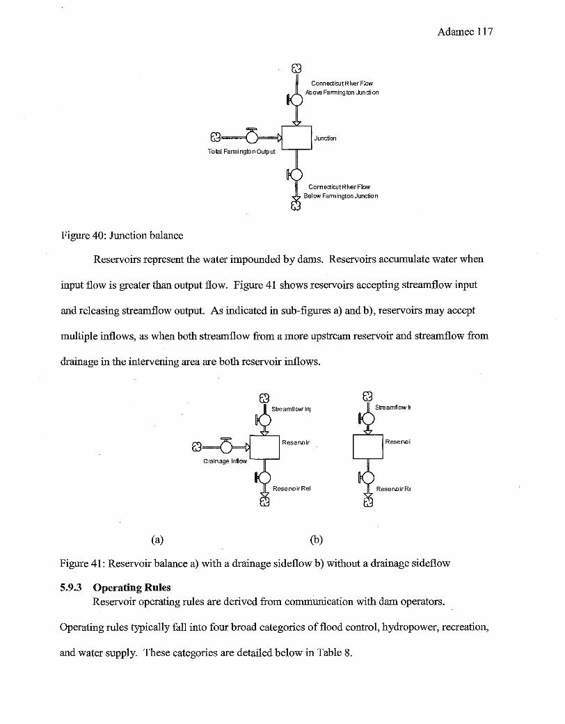
Figure 40: Junction balance

Connecticut River Flow Above Farmington Junction

Junction

ConnecticutRiverFiow Be! ow Farmington Junction

Adamec 117

Reservoirs represent the water impounded by dams. Reservoirs accumulate water when

input flow is greater than output flow. Figure 41 shows reservoirs accepting streamflow input

and releasing streamflow output. As indicated in sub-figures a) and b), reservoirs may accept

multiple inflows, as when both streamflow from a more upstream reservoir and streamflow from

drainage in the intervening area are both reservoir inflows.

(a) (b)

Figure 41: Reservoir balance a) with a drainage sideflow b) without a drainage sideflow

5.9.3 Operating Rules Reservoir operating rules are derived from communication with dam operators.

Operating rules typically fall into four broad categories of flood control, hydropower, recreation,

and water supply. These categories are detailed below in Table 8.

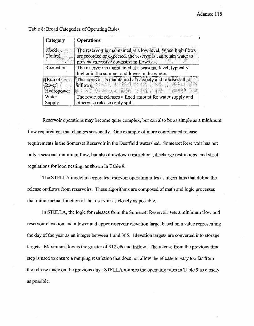
Adamec 118

Table 8: Broad Categories of Operating Rules

Category Operations

F\bod the~reservdlr is maintairied at a low leveL When liigfi flows Control are recorded ~or expected, the reservoirs can retain water to

prevent exces&ive downstrelpll flows. Recreation The reservoir is maintained at a seasonal level, typically

higher in the summer and lower in the winter. [Rundf The reservoir is ~aintained at capacity and r~ledses all River] 'inflows. :~;

flydropo\Ver . ' . . Water The reservoir releases a fixed amount for water supply and Supply otherwise releases only spill.

Reservoir operations may become quite complex, but can also be as simple as a minimum

flow requirement that changes seasonally. One example of more complicated release

requirements is the Somerset Reservoir in the Deerfield watershed. Somerset Reservoir has not

only a seasonal minimum flow, but also drawdown restrictions, discharge restrictions, and strict

regulations for loon nesting, as shown in Table 9.

The STELLA model incorporates reservoir operating rnles as algorithms that define the

release outflows from reservoirs. These algorithms are composed of math and logic processes

that mimic actual function of the reservoir as closely as possible.

In~ STELLA, the logic for releases from the Somerset Reservoir sets a minimum flow and

reservoir elevation and a lower and upper reservoir elevation target based on a value representing

the day of the year as an integer between I and 365. Elevation targets are converted into storage

targets. Maximum flow is the greater of 312 cfs and inflow. The release from the previous time

step is used to ensure a ramping restriction that does not allow the release to vary too far from

the release made on the previous day. STELLA mimics the operating rules in Table 9 as closely

as possible.

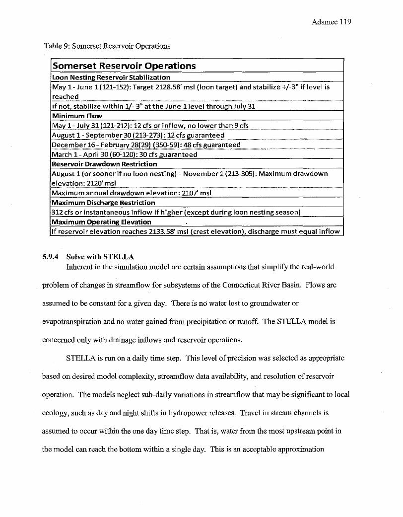
Adamec 119

Table 9: Somerset Reservoir Operations

Somerset Reservoir Operations loon Nesting Reservoir Stabilization

May 1- June 1 (121-152): Target 2128.58' msl (loon target) and stabilize +/-3" if level is

reached --·~·~~· "'" ---~~- --· ---~-·-·- ---~ ~----- ·-----~

if not, stabilize within 1/- 3" at the June 11evel through July 31

Minimum Flow

May 1- July 31 (121-212): 12 c!s or inflow, no lowert_llan 9 cfs u'" ·- -

August 1- S~_pt~mber 30 (213-273): l? cfs guarante.~~- -- ~--~

_December 16_~_£~~~uary 28(29) (350-~~):48 cfs guara_'!~eed -" ~ -March 1- April 30 {60-120): 30 cfs guaranteed

Reservoir Drawdown Restriction

August 1 (or sooner if no loon nesting)- November 1 (213-305): Maximum drawdown

~~vat! on: 2120' msl -~- ~·-- --- "'- """'~' ----- ---

Maximum annual drawdown elevation: 2107' msl

Maximum Discharge Restriction

312 cfs or instantaneous inflow if higher (except during loon nesting season)

Maximum Operating Elevation

If reservoir elevation reaches 2133.58' msl (crest elevation), discharge must equal inflow

5.9.4 Solve with STELLA Inherent in the simulation model are certain assumptions that simplifY the real-world

problem of changes in streamflow for subsystems of the Connecticut River Basin. Flows are

assumed to be constant for a given day. There is no water lost to groundwater or

evapotranspiration and no water gained from precipitation or runoff. The STELLA model is

concerned only with drainage inflows and reservoir operations.

STELLA is run on a daily time step. This level of precision was selected as appropriate

based on desired model complexity, streamflow data availability, and resolution of reservoir

operation. The models neglect sub-daily variations in streamflow that may be significant to local

ecology, such as day and night shifts in hydropower releases. Travel in stream channels is

assumed to occur within the one day time step. That is, water from the most upstream point in

the model can reach the bottom within a single day. This is an acceptable approximation

Adamec 120

because travel time within a single watershed is often significantly less than one day. As long as

travel time is less than one day, instantaneous travel in a daily time step model is appropriate.

For travel along the Connecticut River, where travel time exceeds one day, delays may need to

be added in ordered to more accurately time streamflow.

5.9.5 Input The inputs to the simulation models are daily upstream input streamflow and drainage

input to reservoirs. Inputs are currently drawn primarily from unregulated USGS gages.

Occasionally streamflow from the Army Corps or from preliminary SYE measurements are used.

Not all of the necessary input data is available. When possible, real data is used. When real data

is not available, the closest unregulated USGS streamgage with a reliable record over the period

of interest is scaled by a drainage area ratio and used instead. Daily streamflow time series are

imported to STELLA from Excel files. Input sources to each model are recorded in Table 10.

The time period that the simulation model can be run over is constrained by the time

period of streamflowinput. Based on input, the current models run over slightly different time

periods. In the future, model inputs will be SYE streamflows and will run over the time period

of provided SYE data.

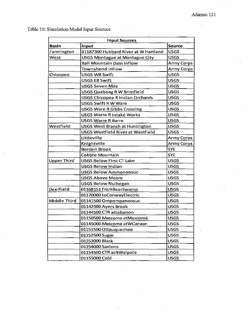
Adamec 121

Table I 0: Simulation Model Input Sources

Input Sources

Basin Input Source

Farmington 01187300 Hubbard River at W Hartland USGS

West USGS Montague at Montague City USGS

Ball Mountain Dam Inflow Army Corps

Townshend Inflow Army Corps

Chicopee USGS WB Swift USGS

USGS EB Swift . USGS

USGS Seven Mile USGS

USGS Quaboag R W Brimfield USGS

USGS Chicopee R Indian Orchards USGS

USGS Swift R W Ware USGS

USGS Ware R Gibbs Crossing USGS

USGS Warre R Intake Works . USGS

USGS Warre R Barre USGS

Westfield USGS West Branch at Huntington USGS

USGS Westfield River at Westfield USGS

Littleville Army Corps

Kn i ghtvi II e Army Corps

Borden Brook SYE

Cobl;>le Mountain SYE

Upper Third USGS Below First CT Lake USGS

USGS Below Indian USGS

USGS Below Ammonoosuc USGS

USGS Above Moore USGS

USGS Below Nulhegan USGS

Deerfield 01168151 fromBearSwamp USGS

01170000 toConwayEiectric USGS

Middle Third 01141500 Ompompanoosuc USGS

01142500Ayers Brook USGS

01144500 CTR atlebanon USGS

01150500 Mascoma atMascoma USGS

01145000 Mascoma atWCanaan USGS

01151500 Ottauquechee USGS

01152500 Sugar USGS

01153000 Black USGS

01154000 Saxtons USGS

01154500 CTR atNWal pole USGS

01155000 Cold USGS

Documents

Sub-Daily Multi-Objective Models for Optimizing Hydropower