1    

Style factor timing: An application to the portfolio holdings of US fund managers    

David R Gallagher a,b,c Peter A Gardner d and Camille H Schmidt a,b

Current Draft: July 2013

a Macquarie Graduate School of Management, Macquarie University AUSTRALIA

b Capital Markets CRC Limited, AUSTRALIA c Centre for International Finance and Regulation, AUSTRALIA

d Plato Investment Management, AUSTRALIA ___________________________________________________________________

Abstract

This study develops a style rotation model based on quarterly forecasts of style factor returns,

across four style categories, generated using market and macroeconomic data. The

prescriptions from this model are tested on a sample of US active equity mutual funds’

portfolio holdings. An annual buy-and-hold style timing strategy investing in the factor with

the highest forecast return each quarter achieves an average annual excess return of 7.26%,

significant at the 1% level over 1981-2011. However, a fund-of-fund timing strategy

investing in the funds with the greatest exposure (i.e. the preferred funds) to the style

predicted to outperform over the following year does not generate statistically significant

DGTW-adjusted performance. The lack of performance is primarily because the long-only

funds are by nature unable to fully exploit the long-short style factor returns. This highlights

the issue of using long-short portfolio returns, particularly when evaluating fund

performance. This paper provides information which is particularly relevant to institutional

investment managers, advisors and consultants.

Keywords Mutual funds, style timing, macroeconomic data, investment performance, stock holdings ___________________________________________________________________________  

Corresponding author:

Camille Schmidt, Macquarie Graduate School of Management, Macquarie University,

Sydney, NSW, 2109, Australia.

Email: cschmidt@cmcrc.com

2    

Style factor timing: An application to the portfolio holdings of US fund managers    

___________________________________________________________________

Abstract This study develops a style rotation model based on quarterly forecasts of style factor returns,

across four style categories, generated using market and macroeconomic data. The

prescriptions from this model are tested on a sample of US active equity mutual funds’

portfolio holdings. An annual buy-and-hold style timing strategy investing in the factor with

the highest forecast return each quarter achieves an average annual excess return of 7.26%,

significant at the 1% level over 1981-2011. However, a fund-of-fund timing strategy

investing in the funds with the greatest exposure (i.e. the preferred funds) to the style

predicted to outperform over the following year does not generate statistically significant

DGTW-adjusted performance. The lack of performance is primarily because the long-only

funds are by nature unable to fully exploit the long-short style factor returns. This highlights

the issue of using long-short portfolio returns, particularly when evaluating fund

performance. This paper provides information which is particularly relevant to institutional

investment managers, advisors and consultants.

 

Keywords Mutual funds, style timing, macroeconomic data, investment performance, stock holdings ___________________________________________________________________________    

3    

Style factor timing: An application to the portfolio holdings of

US fund managers    Background Since the seminal papers on market timing by Treynor and Mazuy (1966) and Henriksson and

Merton (1981) a number of studies investigate whether investment styles can be timed (Bird

and Casavecchia, 2011; Chen and De Bondt, 2004; Copeland and Copeland, 1999;

Desrosiers, L’Her and Plante, 2004; Kao and Shumaker, 1999; Knewtson et al., 2010; Levis

and Liodakis, 1999). The emphasis has been on the popularised four factors; Market, Size,

Value and/or (to a lesser extent) Momentum (Carhart, 1997; Fama and French, 1993;

Jegadeesh and Titman, 1993). Recently, industry players are focusing on timing the

underlying style factors i.e. ‘Factor Timing’, using fundamental and/or macroeconomic

information. The results indicate that style rotation strategies can exhibit significant timing

ability, which translates into better performance when incorporated into the strategies of their

mutual fund portfolios (Luo et al., 2010; Smith and Malin, 2010). Moreover, Levis and

Liodakis (1999) determine that style consistency is not ideal with style rotation able to

improve fund returns. Similarly, Wermers (2002) finds that style-consistent managers often

underperform their more style-cavalier counterparts. Hence, the purpose of this paper is two-

fold. Firstly, a style rotation model based on market and macroeconomic variables is

developed and tested at the stock level over 1981-2011. Secondly, this paper extends the

academic research in this area by testing the prescriptions from the model on the portfolio

holdings of a large sample containing 1856 US active equity mutual funds from 1981-2010.

As a result, information as to whether a mutual fund-of-funds (FoF) timing strategy is

implementable is provided. We define a FoF as a fund which invests in other mutual funds.

The academic literature to date focuses on determining whether individual styles can be

timed and whether fund managers (in the US and globally) exhibit market and/or style timing

skill (Bollen and Busse, 2005; Daniel, Grinblatt, Titman and Wermers (DGTW), 1997;

Glassman and Riddick, 2006; Kacperczyk, Van Nieuwerburgh and Veldkamp 2011; Kao,

Cheng and Chan, 1998; Shukla and Singh, 1997; Swinkels and Tjong-A-Tjoe, 2007). This

paper contributes to the style timing literature by analysing a broader range of investment

styles than previously, across seven style categories; Value, Growth, Quality Growth, Quality

Stability, Momentum, Size and Low Volatility. Previous research supports the extension of

4    

the opportunity set of style factors1. A representative underlying style factor is selected for

analysis from each category. The style timing strategy developed analyses the style factors

simultaneously which contrasts to previous literature in this area which tests timing strategies

for each style separately. In addition, this paper contributes to the mutual fund literature by

analysing whether the portfolio holdings of US mutual funds may be used to implement a

FoF timing strategy. In terms of the portfolio holdings literature DGTW (1997) use the stock

holdings of funds to investigate whether managers have style timing skill, on average.

However, the FoF literature has not been linked to the portfolio holdings literature in order to

test the efficacy of a fund timing strategy2. Thus, this paper provides information relating to

portfolio construction which is particularly relevant to industry parties such as investment

managers, advisors and consultants.

The style factors selected for analysis are; Book-to-Market (B/M), Dividend-to-Price (D/P),

Net Profit Margin (NPM), Return-on-Equity (ROE), Return-on-Asset Variability (ROA

VAR), Momentum (MOM), Size and Stable-minus-Volatile (SMV)3. A multivariate

forecasting model is developed and the independent market/macroeconomic variables4

included are updated every five years i.e. there are six forecasting models used over the

sample period, these are unique to each style factor. As a result, a time-series of forecast style

factor returns is developed for each style factor over 1981-2011. The forecasts are made each

quarter for the return on a 12-month buy-and-hold investment in the style factor commencing

in two quarters’ time. The structure of the strategy is designed to be exploitable by an

investor in real time, therefore only data which are publicly available at each point in time,

over the sample period are used.

Investing in the style which has the maximum forecast each quarter generates an average

annual excess return of 7.26%, which is statistically significant at the 1% level. The

                                                                                                                         1 Ang et al. (2006); Bali et al. (2008); Barbee et al. (1996); Basu (1983); Bird and Casavecchia (2007); Chan et al. (1991); Chan et al. (1998); Chen and Zhang (2007); Clarke et al. (2010); Davis (1994); Dechow and Dichev (2002); Dichev and Tang (2009); Fairfield and Whisenant (2000); Fama and French (1988); Gallagher et al. (2012); George and Hwang (2010); Lakonishok et al. (1994); Lie and Lie (2002); Lockwood and Prombutr (2010); Lui et al. (2007); Mercer (2012); Mohanram (2005); Piotroski (2000); Zhang (2000). 2 Extant mutual FoF research focuses on diversification benefits (Brands and Gallagher, 2005), style characteristics (Stein and Rachev, 2009) and performance (Bertin and Prather, 2009). 3 The forecasts generated for Dividend-to-Price, Net Profit Margin, ROA Variability and Stable-minus-Volatile are not statistically significant when compared to the actual returns. Therefore, these factors are omitted from the stock and fund timing strategy tests. 4 A set of 25 potential market/macroeconomic variables to include in the forecasting models is selected following an in-depth review of the literature. Refer to Appendix A.

5    

strategy’s average return is greater than that for the individual B/M, ROE and SIZE factors;

however the MOM return is slightly higher on average at 7.90%. Although, investing in

MOM incurs a higher level of risk with a Sharpe Ratio which is 17% lower than the timing

strategy. In the interests of minimising turnover, an annual strategy based on the quarterly

forecasts is also tested. It involves investing only in each Qi where 1 ≤ i ≤ 4 e.g. to invest in

each calendar year the Q3 forecasts are used. The returns to investing in any of the four

annual investment options, generates a statistically significant average annual excess return

over the sample period ranging from 6.59-9.01%. In summary, a style timing strategy using a

range of style factors based on market and macroeconomic data is profitable over the sample

period.

Given that a stock selection strategy using the style factor forecasts generates

outperformance, testing whether a timing strategy using the mutual funds based on the style

forecasts generates outperformance is justified. In Q3 of each year t5 a weighted-average

quintile rank (WRankj,t) is computed for each fund j based on its stock holdings in order to

identify the funds which have the greatest exposure to the style factor which has the highest

forecast. Funds are sorted into quintiles based on their exposure to the preferred style as

indicated by WRankj,t in Q3 of each year t. The first year for which holdings data is available

is 1980 thus portfolio formation occurs from 1980-2009. The average returns to the quintiles

are examined over year t+1 i.e. over 1981-2010. Quintile 5 (1) contains funds with the

greatest (lowest) exposure to the preferred style i.e. the preferred (unpreferred/out-of-favour)

funds. The average annual market-adjusted and DGTW-adjusted returns are all statistically

insignificant. Thus, a style timing strategy at the aggregate fund level (i.e. from a FoF

management perspective) does not generate statistically significant outperformance over the

sample period.

Further investigations as to why the performance identified at the stock level does not

translate to the fund level are conducted. These indicate that the result is primarily due to the

fact that the funds are characterised as long-only and thus unable to attain the long-short style

factor return. However, a timing strategy using long-only style factor forecasts does not prove

to be viable. It follows that the use of long-short style factor portfolios in relation to long-

                                                                                                                         5 Thus, an annual strategy is tested using the Q3 forecasts which cover the following calendar year.

6    

only mutual funds in order to undertake tasks such as performance evaluation may not be

appropriate.

The remainder of this paper is organised as follows; the subsequent two sections outline the

data used and relevant summary statistics, respectively; methodology describes the research

methodology developed and then the results are discussed, finally concluding remarks are

provided.

Data

Style factor data

The style factors considered for inclusion in this study are selected following a review of the

academic literature. Table 1 outlines the 19 variables considered- within the value, growth,

quality, momentum, size and low volatility categories- and how each variable is calculated.

The required stock price and accounting data are sourced from CRSP and Compustat,

respectively via Wharton Research Data Services (WRDS).

INSERT TABLE 1

The style factors are constructed in a similar fashion to the Factor Mimicking Portfolios of

Chan, Karceski and Lakonishok (1998), which are inspired by the work of Fama and French

(1993). All common stocks listed on the NYSE, AMEX and NASDAQ are included;

however stocks are assigned to portfolios based on the breakpoints for NYSE stocks only.

The style factors which are constructed using accounting metrics are calculated as follows; in

June of each year t firms are sorted into quintiles based on the value of the metric in question

for the fiscal year ending in year t-1. Returns are then computed from July of year t to June of

year t+1. For the value metrics, firms with zero or negative values of the numerator are

excluded. The value and growth factors are constructed as the difference between the value-

weighted average return of firms in the top quintile and the value-weighted average return of

those in the bottom quintile. The quality factors may be considered as two distinct groups;

quality growth factors; Return-on-Equity (ROE), Return-on-Assets (ROA) and Operating

Cash Flow (OCF) and quality stability factors; Leverage (LEV), Sales Growth Variability

(SG VAR) and ROA Variability (ROA VAR). Financial firms (SIC 6000-6999) are excluded

from the quality portfolios as metrics such as leverage may have a different meaning than

those for nonfinancial firms (Kisgen, 2009). The quality growth factors are calculated as per

7    

the value and growth factors. Whereas, the quality stability factors are calculated as the

difference between the value-weighted average return of firms in quintiles one to four and the

value-weighted average return of those in the top quintile. This method is used for these

stocks as the performance relationship is one-sided with firms in the top quintile experiencing

poor performance; however stocks in the bottom quintile do not experience strong

performance.

Similarly, the size factor is based on assigning stocks into portfolios using the value of

market equity as at June of each year t. Returns are then computed from July of year t to June

of year t+1. The size factor is constructed as the difference between the value-weighted

average return of firms in the bottom quintile and the value-weighted average return of those

in the top quintile.

The momentum factor is calculated in a similar vein to the Carhart (1997) PR1YR factor. It is

constructed as the value-weighted average of firms with the highest 20 percent 11-month

returns lagged one month minus the value-weighted average of firms with the lowest 20

percent 11-month returns lagged one month. Portfolios are rebalanced monthly.

Recently, the academic literature emphasises that portfolios created from stocks with low

idiosyncratic volatility have higher returns than those comprising stocks with high

idiosyncratic volatility (Ang et al., 2006). The low volatility factor; stable-minus-volatile

(SMV) is thus created as the value-weighted average return to the lowest quintile of stocks

based on historical idiosyncratic volatility minus the value-weighted average return to the

highest quintile of stocks based on historical idiosyncratic volatility. Quintiles are formed at

the end of each month and weighted by market-capitalisation at the portfolio formation date.

Historical idiosyncratic volatility is calculated each month as the standard deviation of the

error term, over the prior 60-months, from an OLS regression of the stock’s return in excess

of the risk-free rate on the market return in excess of the risk-free rate, this is consistent with

Clarke et al. (2010).

The 19 factors described above are a potential list of factors to include as the style returns to

be forecast. In order to narrow down the factors for inclusion in the main part of this study a

representative factor is selected from the Value, Growth, Quality Growth and Quality

Stability categories. Chan et al. (1998) emphasise that the importance of a style factor is

directly proportional to the standard deviation of its returns. Thus, the representative style

8    

factors selected are those which had the greatest standard deviation over the forecast period

(1981-2011). The chosen factors are as follows; D/P for Value, NPM for Growth, ROE for

Quality Growth and ROA VAR for Quality Stability. Furthermore, B/M is included in the

Value category given its prominence in the academic literature. Therefore, the eight style

factors’ returns which are forecast are: D/P, B/M, NPM, ROE, ROA VAR, MOM, Size and

SMV.

Market and macroeconomic data

The academic literature emphasises a myriad of market and macroeconomic variables as

relevant for stock and fund returns. A comprehensive list of 25 potential variables to include

as independent variables in the forecasting models is provided in Appendix A. Furthermore,

Appendix B provides summary statistics for the variables.

The Bureau of Economic Analysis (BEA) has made a number of ex-post revisions to the

export and import data used to compute the Balance of Trade (BOT). Given that the ex-post

data is not available ex-ante to investors the original data are collected from the historical

Survey of Current Business publications. The unemployment rate data are original data. The

output gap is computed following Cooper and Priestley (2009) who collect original industrial

production data in order to calculate the output gap. The authors state that the results are not

affected when using either the revised or original data. Therefore, use of the revised data for

industrial production to compute the output gap in this paper is not considered an issue. In

order to minimise the impact of revisions for the other variables the approach Pesaran and

Timmerman (1995) use is followed. Specifically, for the remaining economic variables a

moving average over the prior 4 quarters is first computed for each quarter, and then the year-

on-year change is calculated.

Mutual fund holdings data

The dataset used is created by merging the Thomson Reuters Mutual Fund Common Stock

Holdings6 (s12) Database with the CRSP Mutual Fund Database (CMFD), using MFLINKS.

Refer to Appendix C for a detailed description of the dataset construction. The s12, CMFD

and MFLINKS tables which facilitate the data merge are all sourced from WRDS. The s12

                                                                                                                         6Also known as the CDA/Spectrum s12 database.

9    

data is sourced from the SEC N-30D filings which funds are required to file semi-annually

with the SEC. Up until 1985 funds were required by the SEC to file this data on a quarterly

basis (WRDS, 2008). Although, about 60% of funds continue to provide this data quarterly

(WRDS, 2012). The s12 database contains quarterly stock holdings data for US mutual funds

and the CMFD contains monthly fund returns as well as fund characteristics. This study is

interested in US active equity fund managers thus various exclusions are made to both

datasets.

Firstly, only funds with the following self-stated investment objective classifications are

included: Aggressive Growth (IOC=1), Growth (IOC=2) and Growth and Income (IOC=3).

Following Kacperczyk, Sialm and Zheng (2008), funds which held less than 10 stocks and

with portfolio assets less than $5m in assets as at the end of the month prior are also removed.

The s12 dataset contained 2409 unique funds prior to the merge with the CMFD, after

merging the datasets there are 2047 unique funds, thus 85% of the funds are linked.

Subsequent to merging the two databases a manual check of the funds’ names was

undertaken to ensure misclassified funds are not included (Ali, Chen, Yao and Yu, 2008)7.

There are 2047 unique funds in the merged dataset after removing the misclassified funds, of

which there are 191 in total, the final sample contains 1856 funds over 1980-2010.

Descriptive statistics Style factors

Table 2 provides a summary of the annualised average monthly returns to the style factors

over the complete sample period and various subset periods.

INSERT TABLE 2

In summary, the various style factors perform differently to an extent within the style

categories but clearly over time and in differing market conditions. Therefore, employing a

time-series forecasting model based on these style factors is warranted given that their

performance exhibits time-varying characteristics which may be exploited.

                                                                                                                         7 Funds in the following categories are removed from the sample; Passive funds (n=72), Foreign-based and US-based international funds (n=62), real estate funds (n=29), balanced funds (n=15), variable annuity funds (n=10), convertible funds (n=1) and options funds (n=2).

10    

Mutual fund sample

Table 3 reports summary statistics for the sample of US active equity mutual funds examined

over 1980-2010. Average values of fund characteristic variables and returns are provided, the

median is in parentheses. The number of stocks held by the funds has increased, on average,

from about 70 stocks over 1980-1990 to 111 over 2001-2010. The average age of the funds

was 15 years over the complete sample period. ‘Turnover’ is an annual variable which

represents the minimum (of aggregated sales or aggregated purchases of securities), divided

by the average 12-month Total Net Assets of the Fund. Turnover remained relatively stable

over the sample period with the average oscillating around 80%.

INSERT TABLE 3

‘Expenses’ represents the annual expense ratio, which was approximately 1% over 1980-

1990 increasing to about 1.25% over 1991-2000 and 2001-2010. ‘Equity Prop.’ is the average

proportion of the fund that is invested in common equity and it's calculated over the life of

the fund. The majority of the funds’ assets are invested in common equity, i.e. 87% over

1980-2010, which is not surprising given the data screens applied. ‘TNA’ is the fund's month

end Total Net Asset Value, in millions. TNA have grown over the sample period with the

most dramatic increase of approximately 150% between 1980-1990 and 1991-2000.

‘Total Load’ is the sum of the front and rear loads, reported annually, the average Total Load

fell from 3.5% over 1980-1990 to 0.87%, a decrease of 300%. The average Total Load

experienced a further decrease settling at an average of 0.34% over 2001-2010. Management

Fee (Mgt Fee) is only available from 1998-2010 and is the ratio of Management Fee ($)

divided by Average Total Net Assets ($) reported as a percentage. Management Fees were

very stable with the same mean and median reported over 1998-2001 and 2001-2010.

‘CRSP Raw Ret’ is the annual CRSP fund return including distributions (dividends and

capital gains) before total expenses. ‘CRSP Net Ret’ is the annual CRSP fund return from

CRSP including distributions (dividends and capital gains) after total expenses. The annual

mean is the simple compound of the 12 monthly means for all funds existing in each month.

‘Raw Holdings Ret’ is the annual raw fund return calculated using the quarterly stock

11    

holdings from the s12 database. The annual mean is the simple compound of the four

quarterly means for all funds existing in each quarter. ‘DGTW-adj. Ret’ is the annual excess

fund return whereby the return of each stock in the portfolio has been adjusted by the return

on a portfolio of stocks with similar book-to-market, size and momentum characteristics.

Value-weighted8 returns are provided.

The raw/net average returns are comparable in magnitude and follow a similar pattern over

the three sub-periods. There is a clear fall in returns over 2001-2010, which is not surprising

given that this period encompasses the tech wreck and GFC. Overall, the sample of mutual

funds did not generate outperformance with an average DGTW-adjusted return over the

complete period of -0.04%. Small positive excess returns of 0.69% and 0.77% are reported

over 1980-1990 and 1991-2000, respectively. However, over 2001-2010 funds incurred an

average annual excess return of -1.66%.

Methodology Selecting independent variables

In order to identify the market/macroeconomic variables with the greatest predictive ability a

series of univariate regressions of each style factor on each market/macroeconomic variable

are run in a similar manner to Kao and Shumaker (1999). Specifically, the annual return for

each style factor (SF) is regressed on the quarterly value of each market/macroeconomic

variable (EV) lagged two quarters. The use of the second lag is to ensure that the economic

data is available prior to the start of the investment horizon being forecast, which is consistent

with Cooper and Priestley (2009). The annual SF returns are calculated as the simple

compound of the relevant monthly SF returns, using value-weighted portfolios of stocks,

based on market-capitalisation as at the end of the month prior.

𝑆𝐹!,!!!!! =  ∝!,!  +  𝛽!,!𝐸𝑉!,!!! +  𝜀!,! (1)

Fama and French (1992) emphasise that the pre-1962 data on Compustat suffer from a

serious selection bias as they are tilted toward large historically successful firms.

Furthermore, the Book Value of Shareholders’ Equity is not available before 1962, which is

                                                                                                                         8 The returns are similar when equal-weighting is used.

12    

an input for the computation of ROE. Therefore, the start of the historical period ensures the

sample is not affected by this bias and that data for all of the SFs is available.

The approach used to generate quarterly forecasts of the performance of each SF for the

following 12 months over 1981-2011 involves first segregating the data into six subsets.

Therefore, six unique forecasting models are used to forecast the return of each SF over the

next five years (six years for Subset 6). Within these subsets regressions are run over six

separate rolling historical periods for each SF in order to select the EVs to be used in the

forecasting model for each SF for the six associated forecasting periods. The periods

associated with Subset 1 are explained in detail.

Firstly, univariate regressions are run on a rolling basis with the first regression using five

years of data i.e. Q1 1964 – Q3 1968 and then the historical period increases iteratively by

one quarter with the final regression using 15 years of data i.e. Q1 1964 – Q3 1978.

Therefore, the historical period ends with the EV for Q3 1978 forecasting the SF return over

Q1-Q4 1979, which ensures there is no overlap with the period for which the forecasts are

generated i.e. Q1 1981- Q4 1985.

The EVs included in the forecasting model are selected based on the results of these

univariate regressions. Selection is based on a frequency count of the number of significant t-

statistics (at a 5% confidence level) for beta for each EV. Firstly, all EVs with a significant

beta count of at least 40% of the total are identified. Secondly, the correlations between these

EVs over the complete historical period are computed. Starting at the lowest count end, if the

correlation between two EVs is 0.60 or greater then only the EV with the higher count is

retained. If two EVs have the same count then the EV with the more favourable correlations

with the other EVs selected for inclusion in the forecasting model is retained. Favourability is

determined as follows. The two correlated EVs are compared in relation to each EV selected

for inclusion in the forecasting model. The EV which has the smallest positive/largest

negative correlation with each EV is given a score of 1 and the other EV a score of 0. The

most favourable EV is the one with the greatest total score based on these comparisons. If

their scores are even then the EV with the smallest average positive or largest average

negative correlation across the EVs selected for inclusion in the forecasting model is selected.

Furthermore, if all three spread variables are selected: book-to-market spread, market-to-book

spread and value spread then only the one with the higher count is retained. If two spread

13    

variables have the same count then the same process detailed above is followed to select the

one to include in the model.

Forecasting style factor returns

In order to obtain a forecast return for each style factor, an econometric forecasting model is

used. It is adapted from the forecasting model used by Bird and Casavecchia (2011) to

forecast the value premium for European stocks.

Et(Ft +2) = 𝛼! +  𝜑!𝐹! +   𝛽!,!𝑍!,!!!!! (2)

where Et(Ft+2) is the expected value in quarter t of the factor return for the 12 months

commencing at the start of quarter t+2,  𝛼! is the intercept in quarter t, 𝜑!𝐹!  represents the

sensitivity to the SF return for the 12 months ending in quarter t and 𝛽!,!𝑍!,!!!!!  represents

the sum of the sensitivity in quarter t to the jth lagged market/macroeconomic variable Z.

The forecasting regression model is run on a rolling basis initially using the previous 15 years

of data. In relation to Subset 1, the first regression is run using the EVs selected for inclusion

and the associated SF returns from Q3 1964 – Q2 1979 (the dependent variable associated

with the Q2 1979 EV’s is the SF return from Q4 1979-Q3 1980). To ensure there is no

hindsight bias the parameter estimates obtained are then applied to the SF return for the 12

months ending with Q3 1980 and EV values for Q3 1980 to obtain the forecast for Q1 1981,

which is for the 12 month return from Q1-Q4 1981. The last regression is run using the

selected EVs and the associated SF returns from Q3 1964-Q1 1984. The parameter estimates

obtained are applied to the EV values for Q2 1985 to obtain the forecast for Q4 1985.

Table 4 provides a summary of the model fit statistics for a regression of the forecast SF

returns generated using the model above versus the actual SF returns over 1981-2011.

INSERT TABLE 4

14    

The forecasts generated for B/M9 and SIZE are the strongest over the complete sample

period. Specifically, the forecasts for these two styles are statistically significant at the 1%

level and the adjusted R2 values are moderate10 at 10.78% and 8.69%, respectively. The

forecasts for MOM and ROE are also statistically significant at the 5% level with adjusted R2

values of 4.63% and 4.26%, respectively. Therefore, all further tests will only use these four

style factors which had statistically significant forecasts.

The Mean Absolute Error (MAE) for these four style factors ranges from 15% for B/M to

22% for ROE. Furthermore, the Root Mean Squared Error (RMSE) ranges from 22% for B/M

to 28% for ROE. This indicates the difficulty to forecast the magnitude of the style factor

returns with a high level of precision. However, Size, MOM and B/M are characterised by the

highest success rates which are 67.77%, 61.98% and 60.33%, respectively. Thus, the style

factor forecast return predicts the direction correctly more often than not. Although, the

success rate for ROE is lower at 48.76%. Please refer to Appendix D for a summary of the

EVs which are included in the forecasting model in each of the six forecasting periods for

B/M, ROE, MOM and Size.

Figure 1 provides a graphical representation of the quarterly forecast SF returns generated

versus the actual SF returns over 1981-2011 for the four SFs.

INSERT FIGURE 1

Panel A shows that the forecasts for B/M are similar to the actuals over the majority of time

period subsets except for during the technology boom and bust and over 2005-2010. The

forecasts fall short of the actual returns which soared over the late 1990s during the time of

the technology boom, which is not surprising given this period was an anomalous market

bubble. Panel B shows that the ROE forecasts over 1995-2000 are well aligned with the

actuals; however there are a series of spikes in the forecasts over the complete period. These

are due to large changes in the EVs which the parameter estimates have not yet adjusted to.

Panel C shows that the MOM forecasts are closest to the actuals over the latter two time

                                                                                                                         9 Five outlier observations (Q3 1999- Q3 2000) which include returns during the technology crash (i.e. Q1 2000- Q4 2001) which commenced in March 2000 have been excluded from the B/M model fit tests. 10 Pesaran and Timmerman (1995) state that an adjusted R2 in this context of 20% is high.

15    

period subsets. Panel D demonstrates that the Size forecasts show a similar pattern to the

actuals overall despite disparity between the two over the late 1990’s and early 2000’s.

Results

Stock selection strategy

Table 5 reports average excess return results for investment strategies based on the four style

factor forecasts over 1981-2011.

INSERT TABLE 5

The results for univariate strategies investing in either the style factor with the maximum

(Max FC) or minimum forecast (Min FC) and a strategy which is long (short) the Max FC

(Min FC) are provided. The 'All Quarters' return is the average actual annual return that is

earned if the investment is made each quarter and held for the following 12 months. The

results for annual strategies developed in the interest of reducing turnover are also provided.

The 'Annual (Qi)' returns are for strategies which invest based on the forecasts made only in

each Qi where 1 ≤ i ≤ 4 over the sample period. E.g. to invest in each calendar year the Q3

forecasts are used.

A strategy which involves investing in the style which has the maximum forecast each

quarter, or using any of the four annual investment options, generates a statistically

significant average annual excess return over the sample period ranging from 6.59% to

9.01%. Conversely, investing in the style factor which has the minimum forecast generates

small negative returns on average, none of which are statistically significant. A long/short

strategy based on the maximum and minimum forecasts generates average excess returns

ranging from 7.13% to 10.14% across the investment options, all of which are statistically

significant except for the Annual Q4 strategy.

The MAE indicates that the difference between the actual SF return and the forecast SF

return is 24% on average for the All Quarters strategy. The RMSE is 29% which further

reflects the difficulty to forecast the magnitude of the SF returns included in the strategy with

a high level of accuracy. However, the direction of the return for the preferred SF is predicted

correctly in more than two-thirds of the quarters. The results for the annual strategies are

similar.

16    

Table 6 provides portfolio characteristics for the individual SFs upon which the timing

strategy is based and the timing strategy.

INSERT TABLE 6

The timing strategy generates an average annual return for ‘All Quarters’ which is higher

than the mean for B/M, ROE and SIZE yet slightly lower than the average return for MOM.

However, given the lower risk associated with the timing strategy the Sharpe Ratio is 17%

higher than that for MOM alone. The return difference is strongest for Size and ROE with the

timing strategy performing about 2% higher on average and this difference is statistically

significant at the 5% level. The Annual Qi strategies show a similar pattern with the timing

strategy generating the highest Sharpe Ratio for Q1, Q2 and Q3 and an equal Sharpe Ratio to

MOM for Q4. Therefore, depending on an investor’s combined risk/return objectives a stock

return timing strategy based on macroeconomic information is fruitful.

Fund selection strategy

Given that a stock selection strategy using the SF forecasts generates outperformance, an

extension is to determine whether a timing strategy using the mutual funds based on the style

forecasts generates outperformance. The annual strategy using Q3 forecasts is selected for

adaptation to the funds as it is the most intuitive given that the forecast periods encompassed

are for calendar year returns over the sample period11.

In order to identify the funds which have the greatest exposure to the style factor which has

the highest forecast in Q3 of each year t a weighted-average quintile rank is computed for

each fund based on its stock holdings.

WRankj,t = 𝑄𝑢𝑖𝑛𝑡𝑖𝑙𝑒  𝑅𝑎𝑛𝑘!,!!!!! ∗𝑊!,!,! (3)

                                                                                                                         11 The results are also generated for a strategy based on the Q2 year t stock holdings and these are quantitatively similar to those presented in the body of this paper. Use of the Q1 year t holdings is not feasible given that the stock quintile allocations does not occur until June of year t and then use of the Q4 year t holdings is not considered relevant given that the fund returns for this strategy occur into year t+2 which is considered too far ahead relative to the stock quintile assignments.

17    

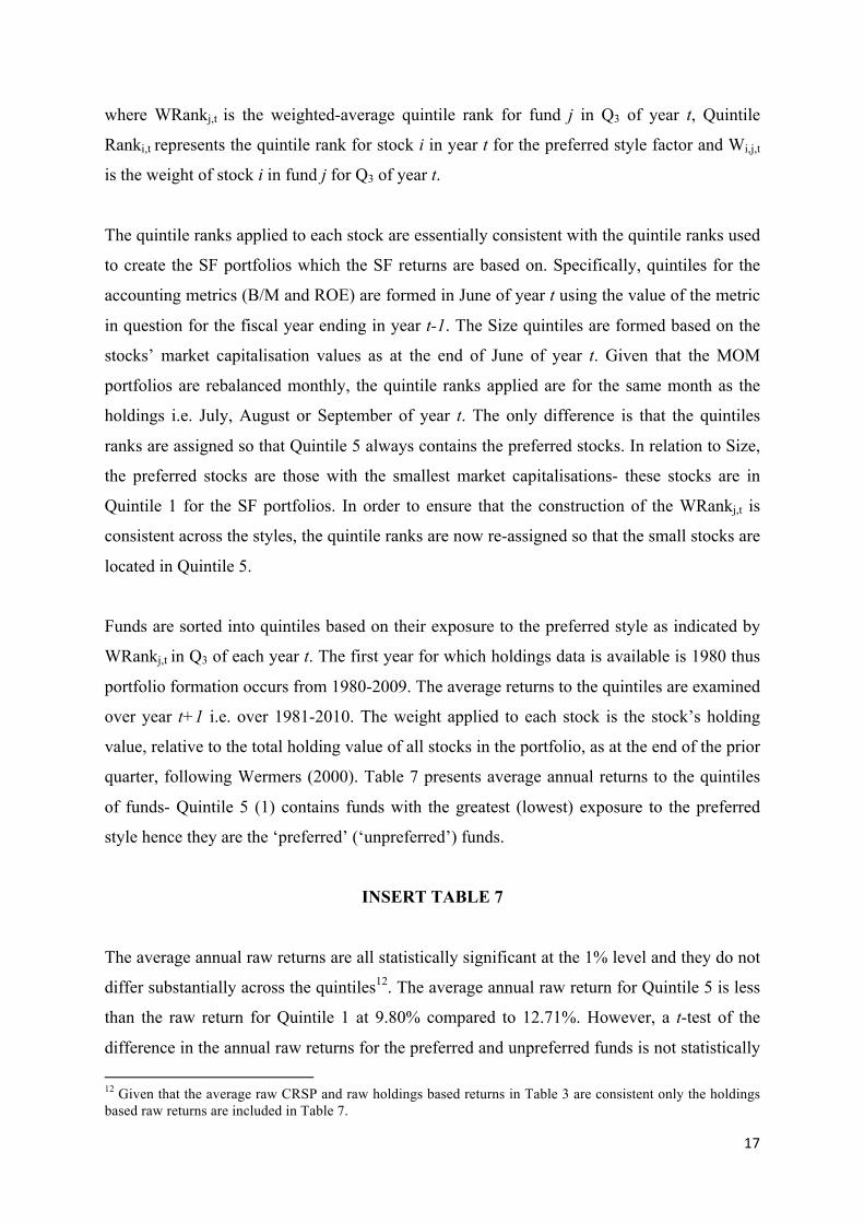
where WRankj,t is the weighted-average quintile rank for fund j in Q3 of year t, Quintile

Ranki,t represents the quintile rank for stock i in year t for the preferred style factor and Wi,j,t

is the weight of stock i in fund j for Q3 of year t.

The quintile ranks applied to each stock are essentially consistent with the quintile ranks used

to create the SF portfolios which the SF returns are based on. Specifically, quintiles for the

accounting metrics (B/M and ROE) are formed in June of year t using the value of the metric

in question for the fiscal year ending in year t-1. The Size quintiles are formed based on the

stocks’ market capitalisation values as at the end of June of year t. Given that the MOM

portfolios are rebalanced monthly, the quintile ranks applied are for the same month as the

holdings i.e. July, August or September of year t. The only difference is that the quintiles

ranks are assigned so that Quintile 5 always contains the preferred stocks. In relation to Size,

the preferred stocks are those with the smallest market capitalisations- these stocks are in

Quintile 1 for the SF portfolios. In order to ensure that the construction of the WRankj,t is

consistent across the styles, the quintile ranks are now re-assigned so that the small stocks are

located in Quintile 5.

Funds are sorted into quintiles based on their exposure to the preferred style as indicated by

WRankj,t in Q3 of each year t. The first year for which holdings data is available is 1980 thus

portfolio formation occurs from 1980-2009. The average returns to the quintiles are examined

over year t+1 i.e. over 1981-2010. The weight applied to each stock is the stock’s holding

value, relative to the total holding value of all stocks in the portfolio, as at the end of the prior

quarter, following Wermers (2000). Table 7 presents average annual returns to the quintiles

of funds- Quintile 5 (1) contains funds with the greatest (lowest) exposure to the preferred

style hence they are the ‘preferred’ (‘unpreferred’) funds.

INSERT TABLE 7

The average annual raw returns are all statistically significant at the 1% level and they do not

differ substantially across the quintiles12. The average annual raw return for Quintile 5 is less

than the raw return for Quintile 1 at 9.80% compared to 12.71%. However, a t-test of the

difference in the annual raw returns for the preferred and unpreferred funds is not statistically                                                                                                                          12 Given that the average raw CRSP and raw holdings based returns in Table 3 are consistent only the holdings based raw returns are included in Table 7.

18    

significant. The raw returns are adjusted using the CRSP value-weighted index including

dividends (CRSP VW). The average market-adj. return for the preferred funds is -1.93%

compared to 0.98% for the unpreferred funds; however these returns are not statistically

distinguishable from 0 (nor are those for the other quintiles). The average annual DGTW-

adjusted return is -1.08% (0.72%) for Quintile 5 (1), although the DGTW-adjusted returns are

also all statistically insignificant. Thus, a style timing strategy at the aggregate fund level

does not generate statistically significant outperformance over the sample period13. Given that

the performance identified at the stock level did not translate to the fund level further

investigations are warranted.

Robustness tests

In addition to the use of the WRankj,t to sort funds into quintiles three alternative methods of

fund selection are discussed in order to determine whether the results are specific to this

approach.

Net exposure rank. Given that the SF returns are generated as the excess of the return to the

preferred stocks relative to the unpreferred stocks a method of fund selection is developed in

a similar vein. Specifically, a Q5_Q1WRankj,t is calculated, which involves calculating each

fund’s exposure to the preferred stocks net of their exposure to stocks least characterised by

the preferred style.

Q5_Q1WRankj,t = 𝑄5  𝑊𝑒𝑖𝑔ℎ𝑡!,! − 𝑄1  𝑊𝑒𝑖𝑔ℎ𝑡!,! (4)

where Q5 Weightj,t = !"#$%&'"  !!!"#$  !"#$  !"#  !"#$%&  !"  !"#$%#&'  !!,!,!

!!!!

!"#$%&'"  !!!"#$  !"#$!,!,!!!!!

and

Q1 Weightj,t = !"#$%&'"  !!!"#$  !"#$  !"#  !"#$%&  !"  !"#$%#&'  !!,!,!

!!!!

!"#$%&'"  !!!"#$  !"#$!,!,!!!!!

The return results for funds sorted into quintiles based on the Q5_Q1WRankj,t are consistent

with the WRankj,t results. The results for this approach are omitted in the interest of brevity.

                                                                                                                         13 A ‘test of perfect information’ is also conducted which involves using the actual SF returns instead of the forecast SF returns to generate the fund application strategy results. The spread of raw returns across the quintiles is clearer, with the highest (lowest) raw returns to funds in Quintile 5 (1). The DGTW-adjusted returns are all statistically insignificant except for a weakly significant return of 1.31%, at the 10% level, for funds in Quintile 5. Thus, even with perfect information the FoF strategy does not generate strong results.

19    

Correlation approach. In order to determine whether the use of the holdings is not adequate14

to identify funds with an affinity to the preferred SF in each period funds are selected based

on the correlation of their monthly raw return from CRSP with the preferred SF portfolio. For

example, if B/M is the preferred style based on the Q3 forecast in 1980 then the correlation of

a fund’s returns with value stocks i.e. Quintile 5 stocks is computed over the 24 months

ending with September 1980. Similarly, if MOM is the preferred style based on the Q3

forecast in 1981 then the correlation of fund’s returns with high price momentum stocks i.e.

Quintile 5 stocks is computed over the 24 months ending with September 1981. The funds are

sorted into quintiles in Q3 of each year t based on the value of this correlation. The results are

consistent with the WRankj,t results.

Selective approach. Given that mutual funds are exposed to a number of SFs in any period a

strategy which isolates funds which are highly exposed to the preferred factor and not to the

other factors is also investigated. A subset of funds which are in Quintile 5 for the preferred

factor and in Quintile 4 or less for all of the other SFs is created. There are 27 funds in this

portfolio on average over the sample period and the average annual DGTW-adjusted return to

these funds is -0.87% and not statistically significant. This is consistent with the main results

presented for the preferred funds and is likely to be due to the fact that the requirement that

the funds are in Quintile 4 or less is still leading to selection of funds which are quite highly

exposed to other style factors15. However, by requiring that funds fall in Quintile 5 for the

preferred factor and Quintile 3 or less for all other SFs a complete time series of returns is not

able to be generated over the sample period as there are not enough funds which meet these

criteria. Furthermore, the average number of funds which meet these criteria for the years in

which returns can be generated is only four and so it is not a large enough sample to render

meaningful results.

Long-only style factor forecasts

                                                                                                                         14 Similarly, in order to determine that the result is not due to a ‘Return Gap’ type influence the results are also generated using a subset of funds for which the number of stocks used to calculate the WRankj,t is within 80-110% of the number of stocks used to calculate the fund’s return (Kacperczyk et al. 2008). The results are indeed consistent. 15 A strategy which maximises the exposure to the preferred style factor and neutralises the exposures to the seven other style factors at the FoF portfolio level is also tested. This involves solving for the weights which generate the global optimum based on these criteria and subject to a number of constraints. The results for this strategy are consistent with the main results.

20    

The investigations above confirm that timing the mutual funds using their stock holdings, and

the SF forecasts as signals, does not generate outperformance. This section seeks to explain

why the stock level performance does not translate to the FoF level.

Given that the sample consists of long-only funds a set of long-only SF forecasts is generated

in order to determine whether a timing strategy using long-only forecasts is better able to

reflect the stock level performance obtainable by the funds. Long-only SFs are constructed by

subtracting the return to the CRSP VW Index from the Top performing portfolio as defined in

the sub-section ‘Style factor data’ in the Data section. The average returns to all style factors

are muted relative to the long-short portfolios (these are omitted in the interests of brevity),

which highlights the outperformance attributable to the short side. The same process is

followed to develop the time-series of SF return forecasts over 1981-2011. However, upon

testing the model fit relative to the actual SF returns, none of the long-only SF forecast

returns are statistically significant. Therefore, it is not possible to forecast the long-only SFs

and develop a stock level or fund level timing strategy using these forecasts. Overall, this is

an interesting result given that the extant literature focuses on long-short SF returns,

particularly to evaluate the performance of long-only mutual funds.

Conclusion This paper develops a model which successfully predicts style factor returns using market

and macroeconomic variables. The US mutual funds which are most exposed to the predicted

“preferred” style factor did not significantly outperform. This is due to outperformance

predominantly coming from the short side of the SF portfolios, which the long-only funds are

by structure are unable to take advantage of. Furthermore, generation of long-only SF

forecasts is unsuccessful. This raises the question as to the appropriateness of the use of long-

short SF returns to assess the performance of long-only mutual funds. However, we leave this

to future research.

Overall, developing a FoF portfolio purely designed to take advantage of style cycles is not a

profitable strategy. The evidence in this paper suggests that the benefits of a timing strategy

are best exploited alternatively. For example, by including a fund implementing a style

timing strategy within a FoF portfolio to augment performance; however verification of this

approach is best left to further research. Developing a base portfolio with specific style

21    

characteristics and then augmenting/adjusting the structure and characteristics of the portfolio

to take advantage of movements in style cycles e.g. by adding a value manager when value is

expected to outperform is an alternative approach also worthy of further research. Moreover,

a FoF could use factor ETFs or futures to gain exposure to different styles more effectively

than by switching managers. Thus, the fund could obtain alpha from their manager in one

style; whilst being exposed to the beta from another style and the factor timing.

Acknowledgements

The authors gratefully acknowledge invaluable comments provided by Nick White and Derek

Mock.

Funding

This research received no specific grant from the Capital Markets Co-operative Research

Centre and Mercer Investments.

References

Ali A, Chen X, Yao T and Yu T (2008) Do mutual funds profit from the accruals anomaly?

Journal of Accounting Research 46(1): 1-26.

Ang A, Hodrick RJ, Xing Y and Zhang X (2006) The cross-section of volatility and expected

returns. The Journal of Finance 61(1): 259-299.

Baker M and Stein JC (2004) Market liquidity as a sentiment indicator. Journal of Financial

Markets 7(3): 271-299.

Baker M and Wurgler J (2006) Investor sentiment and the cross-section of stock returns. The

Journal of Finance 61(4): 1645-1680.

Bali TG, Demirtas, KO and Tehranian H (2008) Aggregate earnings, firm-level earnings, and

expected stock returns. Journal of Financial and Quantitative Analysis 43(3): 657-684.

Banz RW (1981) The relationship between return and market value of common stocks.

Journal of Financial Economics 9(1): 3-18.

22    

Barbee WC Jr, Mukherji S and Raines GA (1996) Do sales-price and debt-equity explain

stock returns better than book-market and firm size? Financial Analysts Journal 52(2): 56-60.

Basu S (1983) The relationship between earnings’ yield, market value and return for NYSE

common stocks: Further evidence. Journal of Financial Economics 12(1): 129-156.

Bertin WJ and Prather L (2009) Management structure and the performance of funds of

mutual funds. Journal of Business Research 62(12): 1364-1369.

Bird R and Casavecchia L (2007) Sentiment and financial health indicators for value and

growth stocks: The European experience. The European Journal of Finance 13(8): 769–793.

Bird R and Casavecchia L (2011) Conditional style rotation model on enhanced value and

growth portfolios: The European experience. Journal of Asset Management 11(6): 375-390.

Bollen NPB and Busse JA (2005) Short-term persistence in mutual fund performance. The

Review of Financial Studies 18(2): 569-597.

Brands S and Gallagher DR (2005) Portfolio selection, diversification and fund-of-funds: A

note. Accounting & Finance 45(2): 185-197.

Campbell JY and Vuolteenaho T (2004) Inflation illusion and stock prices. National Bureau

of Economic Research Working Paper No. 10263.

Carhart M (1997) On persistence in mutual fund performance. The Journal of Finance 52(1):

57-82.

Cevik EI, Korkmaz T and Atukeren E (2012) Business confidence and stock returns in the

USA: A time-varying Markov regime-switching model. Applied Financial Economics 22(4):

299-312.

Chan LKC, Hamao Y and Lakonishok J (1991) Fundamentals and stock returns in Japan. The

Journal of Finance 46(5): 1739-1764.

23    

Chan LKC, Karceski J and Lakonishok J (1998) The risk and return from factors. Journal of

Financial and Quantitative Analysis 33(2): 159-188.

Chen HL and De Bondt W (2004) Style momentum within the S&P-500 index. Journal of

Empirical Finance 11(4): 483-507.

Chen NF, Roll R and Ross SA (1986) Economic forces and the stock market. The Journal of

Business 59(3): 383-403.

Chen P and Zhang G (2007) How do accounting variables explain stock price movements?

Theory and evidence. Journal of Accounting and Economics 43(2-3): 219-244.

Clarke RG, De Silva H and Thorley S (2010) Know your VMS exposure. The Journal of

Portfolio Management 36(2): 52-59.

Cohen RB, Polk C and Vuolteenaho T (2003) The value spread. The Journal of Finance

58(2): 609-642.

Cooper I and Priestley R (2009) Time-varying risk premiums and the output gap. The Review

of Financial Studies 22(7): 2801-2833.

Copeland MM and Copeland TE (1999) Market timing: Style and size rotation using the

VIX. Financial Analysts Journal 55(2): 73-81.

Daniel K, Grinblatt M, Titman S and Wermers R (1997) Measuring mutual fund performance

with characteristic-based benchmarks. The Journal of Finance 52(3): 1035-1058.

Davis, JL (1994) The cross-section of realised stock returns: The pre-COMPUSTAT

evidence. The Journal of Finance 49(5): 1579-1593.

Davis JL, Fama EF and French KR (2000) Characteristics, covariances, and average returns:

1929-1997. The Journal of Finance 55(1): 389-406.

24    

Dechow P and Dichev I (2002) The quality of accruals and earnings: The role of accrual

estimation errors. The Accounting Review 77(1): 35-59.

Desrosiers S, L’Her J and Plante J (2004) Style management in equity country allocation.

Financial Analysts Journal 60(6): 40-54.

Dichev I and Tang V (2009) Earnings volatility and earnings predictability. Journal of

Accounting and Economics 47(1-2): 160-181.

Elton EJ, Gruber MJ and Blake CR (1995) Fundamental economic variables, expected

returns, and bond fund performance. The Journal of Finance 50 (4): 1229-1256.

Fairfield P and Whisenant S (2000) Using fundamental analysis to assess earnings quality:

Evidence from the Center for Financial Research and Analysis. Journal of Accounting,

Auditing and Finance 16(4): 273-295.

Fama EF and French KR (1988) Dividend yields and expected stock returns. Journal of

Financial Economics 22(1): 3-25.

Fama EF and French KR (1992) The cross-section of expected returns. The Journal of

Finance 47(2): 427-465.

Fama EF and French KR (1993) Common risk factors in the returns on stocks and bonds.

Journal of Financial Economics 33(1): 3-56.

Ferson WE and Schadt RW (1996) Measuring fund strategy and performance in changing

economic conditions. The Journal of Finance 51(2): 425-461.

Flannery MJ and Protopapadakis AA (2002) Macroeconomic factors do influence aggregate

stock returns. The Review of Financial Studies 15(3): 751-782.

Gallagher DR, Gardner P, Schmidt C and Walter TS (2012) Portfolio quality and mutual fund

Performance. Working Paper, Available at: http://ssrn.com/abstract=2151658 (accessed 15

October 2012).

25    

George T and Hwang C (2010) A resolution of the distress risk and leverage puzzles in the

cross-section of stock returns. Journal of Financial Economics 96(1): 56-79.

Glassman DA and Riddick LA (2006) Market timing by global fund managers. Journal of

International Money and Finance 25(7): 1029-1050.

Henriksson RD and Merton RC (1981) On market timing and investment performance. II.

Statistical procedures for evaluating forecasting skills. The Journal of Business 54(4): 513-

533.

Jegadeesh N and Titman S (1993) Returns to buying winners and selling losers: Implications

for stock market efficiency. The Journal of Finance 48(1): 65-91.

Kacperczyk M, Sialm C and Zheng L (2008) Unobserved actions of mutual funds. The

Review of Financial Studies 21(6): 2379-2416.

Kacperczyk M, Van Nieuwerburgh S and Veldkamp L (2011) Time-varying fund manager

skill. National Bureau of Economic Research Working Paper No. 17615.

Kao GW, Cheng LTW and Chan KC (1998) International mutual fund selectivity and market

timing during up and down market conditions. The Financial Review 33(2): 127 -144.

Kao DL and Shumaker RD (1999) Equity style timing. Financial Analysts Journal 55(1): 37-

48.

Kisgen DJ (2009) Do firms target credit ratings or leverage levels? Journal of Financial and

Quantitative Analysis 44(6): 1323-1344.

Knewtson HS, Sias RW and Whidbee DA (2010) Style timing with insiders. Financial

Analysts Journal 66(4): 1-21.

Lakonishok J, Shleifer A and Vishny RW (1994) Contrarian investment, extrapolation and

risk. The Journal of Finance 49(5): 1541-1578.

26    

Levis M and Liodakis M (1999) The profitability of style rotation strategies in the United

Kingdom. Journal of Portfolio Management 26(1): 73-86.

Lie E and Lie H (2002) Multiples used to estimate corporate value. Financial Analysts

Journal 58 (2): 44-55.

Lockwood L and Prombutr W (2010) Sustainable growth and stock returns. Journal of

Financial Research 33(4): 519-538.

Lu N and Zhang L (2008) The value spread as a predictor of returns. National Bureau of

Economic Research Working Paper No. 11326.

Lui D, Markov S and Tamayo A (2007) What makes a stock risky? Evidence from sell-side

analysts’ risk assessments. Journal of Accounting Research 45(3): 629-665.

Luo Y, Cahan R, Jussa J and Alvarez M (2010) Style rotation- GTAA/signal processing.

Deutsche Bank Securities Inc. Quantitative Strategy Research Paper, North America United

States, 7 September.

Mercer Investment Consulting (2012) Style research analysis- Database, Sydney, Australia.

Mohanram P (2005) Separating winners from losers among low book-to-market stocks using

financial statement analysis. Review of Accounting Studies 10(4): 133–170.

Organisation for Economic Co-Operation and Development (OECD) (1987) OECD leading

indicators and business cycles in member countries 1960-1985. OECD Main Economic

Indicators, Sources and Methods, No. 39 (January).

Pesaran MH and Timmermann A (1995) Predictability of stock returns: Robustness and

economic significance. The Journal of Finance 50(4): 1201-1228.

Pesaran MH and Timmermann A (2000) A recursive modelling approach to predicting UK

stock returns. The Economic Journal 110(460): 159-191.

27    

Piotroski J (2000) Value investing: The use of historical financial statement information to

separate winners from losers. Journal of Accounting Research 38(Supplement): 1-41.

Shukla R and Singh S (1997) A performance evaluation of global equity mutual funds:

Evidence from 1988-95. Global Finance Journal 8(2): 279-293.

Smith R and Malin S (2010) Style timing using macro indicators. JP Morgan, Asia Pacific,

Research Paper, 11 November.

Statman M, Thorley S and Vorkink K (2006) Investor overconfidence and trading volume.

The Review of Financial Studies 19(4): 1531-1565.

Stein M and Rachev ST (2009) Style-neutral funds of funds: Diversification or deadweight?

Journal of Asset Management 11(6): 417-434.

Swinkels L and Tjong-A-Tjoe L (2007) Can mutual funds time investment styles? Journal of

Asset Management 8(2): 123-132.

Treynor JL and Mazuy KK (1966) Can mutual funds outguess the market? Harvard Business

Review 44(4): 131-136.

Wermers R (2000) Mutual fund performance: An empirical decomposition into stock-picking

talent, style, transactions costs and expenses. The Journal of Finance 55(4): 1655-1695.

Wermers R (2002) Matter of style: The causes and consequences of style drift in institutional

portfolios. Working Paper, Available at: http://ssrn.com/abstract=2024259 (accessed 19 June

2012).

Wharton Research Data Services (WRDS) (2008) User’s guide to Thomson Reuters mutual

fund and investment company common stock holdings databases on WRDS, Available at:

http://wrds-

web.wharton.upenn.edu/wrds/support/Data/_001Manuals%20and%20Overviews/_004Th

omson%20Reuters/index.cfm (accessed 16 February 2012)

28    

WRDS (2012) Return gap sample program, Available at: http://wrds-

web.wharton.upenn.edu/wrds/support/Data/_004Research%20Applications/_001Portfolio%2

0Construction%20and%20Benchmarks/_010Return%20Gap/Return_Gap_sas_code.cfm

(accessed 16 February 2012).

Zhang G (2000) Accounting information, capital investment decisions, and equity valuation:

Theory and empirical implications. Journal of Accounting Research 38(2): 271-295.