Embed Size (px)
Citation preview
Studying large networks via local weak limit
theory
Venkat Anantharam
EECS Department
University of California, Berkeley
March 10, 2017
Advanced Networks Colloquium
University of Maryland, College Park
(Joint work with Justin Salez and Payam Delgosha )
Venkat Anantharam Large networks March 10, 2017 1 / 70

Outline
1 A resource allocation problem studied by Hajek
2 Load balancing on graphs
3 The framework of local weak convergence
4 Load balancing on hypergraphs
5 Graph indexed data
6 Universal compression of graphical data
Venkat Anantharam Large networks March 10, 2017 2 / 70
Justin Salez Payam Delgosha
Venkat Anantharam Large networks March 10, 2017 3 / 70

Outline
1 A resource allocation problem studied by Hajek
2 Load balancing on graphs
3 The framework of local weak convergence
4 Load balancing on hypergraphs
5 Graph indexed data
6 Universal compression of graphical data
Venkat Anantharam Large networks March 10, 2017 4 / 70
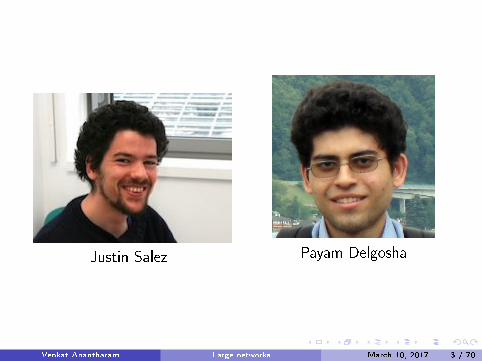
Resource allocation
Consumers above, Resources below
Venkat Anantharam Large networks March 10, 2017 5 / 70

Balanced resource allocation
Let f be a convex function on the nonnegative reals.
Over assignments θ, the objective is to minimize
J(θ) :=M∑i=1
f (∂θ(i)) .
where ∂θ(i) is the load at resource i and M is the number ofresources.
Theorem ( Hajek): The assignment θ minimizes J(θ) i� for allpairs of resources i , i ′ available to consumer u we have θu(i) = 0whenever ∂θ(i) > ∂θ(i ′).
Note that the condition for an assignment to be balanced doesnot depend on f .
Venkat Anantharam Large networks March 10, 2017 6 / 70

Uniqueness of the balanced loads
The assignment θ need not be unique, but ∂θ(i) is unique
1
1
1
1/2
1/21/2
1/2
1/21/2
Venkat Anantharam Large networks March 10, 2017 7 / 70

Many consumers and resources
We want to understand the local environment of a typical agent(consumer, resource) in resource allocation problem with manyagents.
We will �rst describe how this can be done for the basic loadbalancing problem in the case of large sparse graphs .
Venkat Anantharam Large networks March 10, 2017 8 / 70

Outline
1 A resource allocation problem studied by Hajek
2 Load balancing on graphs
3 The framework of local weak convergence
4 Load balancing on hypergraphs
5 Graph indexed data
6 Universal compression of graphical data
Venkat Anantharam Large networks March 10, 2017 9 / 70

Graphs
A graph corresponds to a load balancing problem where eachconsumer has access to two resources.
Each edge is a consumer with one unit of load and has to decidehow to distribute its load between the two vertices that de�nethe edge.
Multiple edges between a pair of vertices are okay.
Venkat Anantharam Large networks March 10, 2017 10 / 70

Load percolationNote that the local structure of the balanced allocation dependson the global structure of the graph, not just on its localstructure.
Figure: Graph A Figure: Graph B
The marked vertex in graph A has the same depth-1neighborhood as the root in graph B .However the induced balanced load is 3
2at each vertex in graph
A and is 45in graph B .
The phenomenon underlying this is called load percolation byHajek.
Venkat Anantharam Large networks March 10, 2017 11 / 70
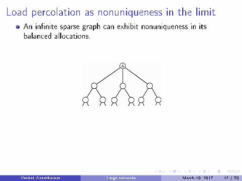
Load percolation as nonuniqueness in the limitAn in�nite sparse graph can exhibit nonuniqueness in itsbalanced allocations.
In this in�nite 3-regular tree, start by assigning the load of eachedge to the vertex that is furthest from the marked vertex.
This gives induced load 1 at all vertices except for the markedone, which has induced load 0.
Venkat Anantharam Large networks March 10, 2017 12 / 70
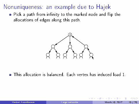
Nonuniqueness: an example due to HajekPick a path from in�nity to the marked node and �ip theallocations of edges along this path.
This allocation is balanced. Each vertex has induced load 1.
Now �ip the allocation of each edge.This is another balanced allocation !! . The induced load ateach vertex is 2.These examples are due to Hajek.
Venkat Anantharam Large networks March 10, 2017 13 / 70

Nonuniqueness: an example due to HajekPick a path from in�nity to the marked node and �ip theallocations of edges along this path.
This allocation is balanced. Each vertex has induced load 1.Now �ip the allocation of each edge.This is another balanced allocation !! . The induced load ateach vertex is 2.These examples are due to Hajek.
Venkat Anantharam Large networks March 10, 2017 13 / 70

Another look at the Hajek counterexample
−→
←−
−→
−→
←−
−→
←−
−→
−→
...
...
...
←−−→ ←−
←−
−→
←−
−→
←−
←−
...
...
...
Venkat Anantharam Large networks March 10, 2017 14 / 70

Hajek's conjectures
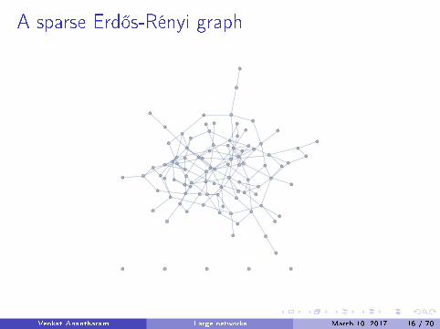
To develop insight into the structure of the balanced loadallocation in large graphs Hajek carried out simulations.
He picked random graphs according to a sparse Erd®s-Rényimodel and studied the corresponding balanced allocations.
Venkat Anantharam Large networks March 10, 2017 15 / 70
A sparse Erd®s-Rényi graph
Venkat Anantharam Large networks March 10, 2017 16 / 70

Numerics on Erd®s-Rényi graphs (Hajek)
αM consumers and M resources; edges picked at random
Venkat Anantharam Large networks March 10, 2017 17 / 70

Numerics on Erd®s-Rényi graphs (Hajek) (cont'd)
Venkat Anantharam Large networks March 10, 2017 18 / 70
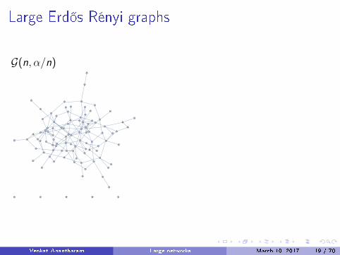
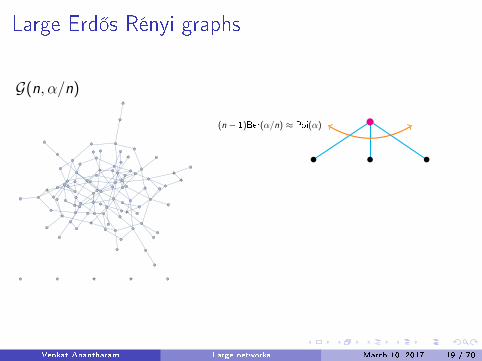
Large Erd®s Rényi graphs
G(n, α/n)
(n − 1)Ber(α/n) ≈ Poi(α)
(n − 3)α2
n2= O(1/n)
Venkat Anantharam Large networks March 10, 2017 19 / 70
Large Erd®s Rényi graphs
G(n, α/n)
(n − 1)Ber(α/n) ≈ Poi(α)
(n − 3)α2
n2= O(1/n)
Venkat Anantharam Large networks March 10, 2017 19 / 70

Large Erd®s Rényi graphs
G(n, α/n)
(n − 1)Ber(α/n) ≈ Poi(α)
(n − 3)α2
n2= O(1/n)
Venkat Anantharam Large networks March 10, 2017 19 / 70

Large Erd®s Rényi graphs
G(n, α/n)
(n − 1)Ber(α/n) ≈ Poi(α)
(n − 3)α2
n2= O(1/n)
Venkat Anantharam Large networks March 10, 2017 19 / 70

The Poisson Galton-Watson tree
Poisson Galton-Watson tree :� Start with a root.� Pick a Poisson (λ) number of neighbors (at depth 1).� For each of these, independently pick a Poisson (λ) number ofneighbors (at depth 2)....Etc.
The local environment of a typical vertex in an Erd®s - Rényigraph converges to a Poisson Galton-Watson tree as M →∞.
Venkat Anantharam Large networks March 10, 2017 20 / 70

A recursive distributional equation
The numerics suggest that there should be a well de�nedlimiting distribution (M →∞) for the induced load (in abalanced allocation) at a typical vertex.
Natural guess: the limiting induced load distribution obeys a�xed point equation (a recursive distributional equation ).
This was conjectured by Hajek.
Venkat Anantharam Large networks March 10, 2017 21 / 70

Our contribution
We verify this conjecture of Hajek as a special case of a broaderresult.
Our results are in the language of local weak convergence ofsequences of graphs, also called the objective method .
In this theory graphs are viewed through the lens of probabilitydistributions on rooted graphs.
Venkat Anantharam Large networks March 10, 2017 22 / 70
What we prove (with Justin Salez)
There is a uniquely de�ned balanced allocation associated to anyprobability distribution on in�nite rooted graphs that can arise asa local weak limit of a sequence of �nite graphs.
The unique balanced allocation on the �nite graphs converges tothe corresponding unique balanced allocation on its local weaklimit.
The induced load distribution at the root in the in�nite limitrooted graph obeys the expected recursive distributionalequation.
Venkat Anantharam Large networks March 10, 2017 23 / 70

Outline
1 A resource allocation problem studied by Hajek
2 Load balancing on graphs
3 The framework of local weak convergence
4 Load balancing on hypergraphs
5 Graph indexed data
6 Universal compression of graphical data
Venkat Anantharam Large networks March 10, 2017 24 / 70

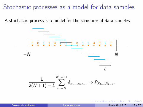
Stochastic processes as a model for data samples
A stochastic process is a model for the structure of data samples.
−N N
0 0 0 0 0 0 0 0 01 1 1 1 1 1
L
1
2(N + 1)− L
N−L+1∑i=−N
δxi ,...,xi+L−1 ⇒ PX0,...,XL−1 .
Venkat Anantharam Large networks March 10, 2017 25 / 70

Stochastic processes as a model for data samples
A stochastic process is a model for the structure of data samples.
−N N
0 0 0 0 0 0 0 0 01 1 1 1 1 1
L
1
2(N + 1)− L
N−L+1∑i=−N
δxi ,...,xi+L−1 ⇒ PX0,...,XL−1 .
Venkat Anantharam Large networks March 10, 2017 25 / 70
Stochastic processes as a model for data samples
A stochastic process is a model for the structure of data samples.
−N N
0 0 0 0 0 0 0 0 01 1 1 1 1 1
L
1
2(N + 1)− L
N−L+1∑i=−N
δxi ,...,xi+L−1 ⇒ PX0,...,XL−1 .
Venkat Anantharam Large networks March 10, 2017 25 / 70

�Empirical distribution� of a marked graph
4
2 3
1
5
6 7
8
G
14
12
14
U2(G )
Venkat Anantharam Large networks March 10, 2017 26 / 70
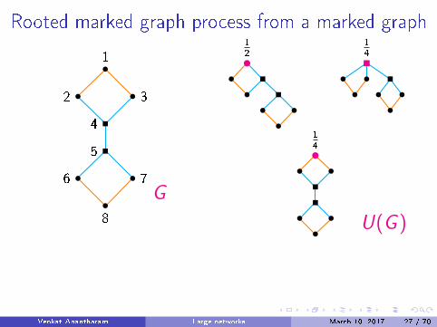
Rooted marked graph process from a marked graph
4
2 3
1
5
6 7
8
G
14
12
14
U(G )
G∗: space of unlabelled marked rooted graphs
A process with values in rooted marked graphs: µ ∈ P(G∗)We will �rst consider the unmarked case.
Venkat Anantharam Large networks March 10, 2017 27 / 70

Rooted marked graph process from a marked graph
4
2 3
1
5
6 7
8
G
14
12
14
U(G )
G∗: space of unlabelled marked rooted graphs
A process with values in rooted marked graphs: µ ∈ P(G∗)We will �rst consider the unmarked case.
Venkat Anantharam Large networks March 10, 2017 27 / 70

Rooted marked graph process from a marked graph
4
2 3
1
5
6 7
8
G
14
12
14
U(G )
G∗: space of unlabelled marked rooted graphs
A process with values in rooted marked graphs: µ ∈ P(G∗)We will �rst consider the unmarked case.
Venkat Anantharam Large networks March 10, 2017 27 / 70

The space of rooted graphs
G∗ denotes the set of locally �nite connected rooted graphsconsidered up to rooted isomorphism.
The distance between two elements of G∗ is 11+r
, where r is thelargest depth of a neighborhood around the root up to whichthey agree.
This distance makes G∗ into a complete separable metric space.
Venkat Anantharam Large networks March 10, 2017 28 / 70
Local weak limit of a sequence of graphs
A �xed �nite graph G corresponds to a probability distributionon G∗ by picking the root at random from the vertices of G .
A sequence of �nite graphs is said to converge in the sense oflocal weak convergence if the corresponding probabilitydistributions on G∗ converge weakly.
The de�nitions extend naturally to marked graphs , i.e. graphs whereeach edge and each vertex carries an element of some other separablemetric space.
Venkat Anantharam Large networks March 10, 2017 29 / 70
The space of (edge, vertex) rooted graphs
G∗∗ denotes the set of locally �nite connected graphs with adistinguished oriented edge, considered up to isomorphism(preserving the distinguished oriented edge).
G∗∗ can be metrized to give a complete separable metric space,just as for G∗.
Venkat Anantharam Large networks March 10, 2017 30 / 70

Moving between G∗ and G∗∗
A function f : G∗∗ 7→ R gives rise to a function ∂f : G∗ 7→ Rvia
∂f (G , o) =∑i∼o
f (G , i , o) .
A probability distribution µ on G∗ gives rise to a measure ~µ onG∗∗ via∫
G∗∗fd~µ =
∫G∗∂fdµ , for all bounded continuous f .
Note that ~µ(G∗∗) = deg(µ) :=∫G∗ deg(root)dµ .
Venkat Anantharam Large networks March 10, 2017 31 / 70
Unimodularity
Given f : G∗∗ 7→ R, de�ne f ∗ : G∗∗ 7→ R via
f ∗(G , i , o) = f (G , o, i) .
A probability distribution µ on G∗ is called unimodular if∫G∗∗
fd~µ =
∫G∗∗
f ∗d~µ , for all bounded continuous f .
It is known that the local weak limit of any sequence of �nitegraphs is unimodular (Aldous and Lyons).
Venkat Anantharam Large networks March 10, 2017 32 / 70
Asymptotic notion of a balanced allocation
A function Θ : G∗∗ 7→ [0, 1] is called an allocation ifΘ + Θ∗ = 1.
An allocation Θ is called a balanced allocation for a givenunimodular µ if for ~µ almost all (G , i .o) it holds that
∂Θ(G , i) < ∂Θ(G , o) =⇒ Θ(G , i , o) = 0 .
Venkat Anantharam Large networks March 10, 2017 33 / 70

Formal statement of the main results
We prove that for any unimodular µ with deg(µ) <∞ there is aΘ0 that is a balanced allocation for µ with the property that itsimultaneously minimizes
∫G∗ f (∂Θ)dµ over allocations Θ for
every convex real valued function f on R+.
Further, Θ0 is µ-almost surely unique.
For any sequence of �nite graphs with local weak limit µ, theempiricial distribution of the induced load in the unique balancedallocation on these graphs converges weakly to the law of ∂Θ0
(for the Θ0 of the limit).
Venkat Anantharam Large networks March 10, 2017 34 / 70

Variational characterization of the limit
Given unimodular µ on G∗ with deg(µ) <∞, de�ne, for eacht ≥ 0,
Φµ(t) :=
∫G∗
(∂Θ0 − t)+dµ .
t 7→ Φµ(t) is the mean-excess function of the almost surelyunique balanced allocation associated to µ.
We have the variational characterization
Φµ(t) = maxf : G∗→[0,1],Borel
{12
∫G∗∗
f̂ d~µ− t
∫G∗fdµ} ,
for each t, where
f̂ (G , i , o) := f (G , i) ∧ f (G , o) .
Venkat Anantharam Large networks March 10, 2017 35 / 70

Intuition behind the variational characterization
The optimizing function is f = 1(∂Θ0 > t).
To check this, observe that
1
2
∫G∗∗
f̂ d~µ =1
2
∫G∗
(∂ f̂ )dµ
=1
2
∫G∗
∑i∼o
1(∂Θ0(G , i) > t and ∂Θ0(G , o) > t)dµ .
Thus ∫G∗
(∂Θ0 − t)+dµ =1
2
∫G∗∗
f̂ d~µ− t
∫G∗fdµ ,
for this choice of f .
Venkat Anantharam Large networks March 10, 2017 36 / 70

Unimodular Galton-Watson treesGiven a probability distribution {π(i) , i ≥ 0} on thenonnegative integers, with �nite mean
∑i iπ(i), de�ne
π̂(i) :=(i + 1)π(i + 1)∑
i iπ(i), i ≥ 0 .
{π̂(i) , i ≥ 0} is also a probability distribution.The unimodular Galton-Watson tree, UGWT(π) is the randomtree constructed as follows: Start with a root and give it arandom number of children (at depth 1) with the number ofchildren distributed as π. For each child, give it a randomnumber of children (at depth 2), the number distributed as π̂,independently. Repeat (using π̂ from now on).Many standard sequences of bipartite graph models, such as thepairing model based on half edges and �xed degree distributionswhich shows up in the theory of LDPC codes, have a unimodularGalton-Watson tree as their local weak limit
Venkat Anantharam Large networks March 10, 2017 37 / 70

Recursive distributional equation characterization
of the limit on unimodular Galton-Watson treesIf µ is the law of UGWT(π), then for every t, we have
Φµ(t) = maxQ=Fπ,t(Q)
{E [D]
2P(ξ1 + ξ2 > 1)− tP(ξ1 + . . .+ ξD > t)} ,
where Fπ,t(Q) is the law of [1− t + ξ1 + . . . + ξD̂ ]10.
Here [a]10 equals 0 if a < 0, 1 if a > 1 and a otherwise. Also, D̂has the law π̂, D has the law π, and the ξi are i.i.d. with law Q.Recall that
t 7→ Φµ(t) :=
∫G∗
(∂Θ0 − t)+dµ ,
characterizes the limiting distribution of the induced load at theroot.The above recursive distributional characterization of is in e�ectthe one conjectured by Hajek.
Venkat Anantharam Large networks March 10, 2017 38 / 70

Intuition behind the RDE
We consider the RDE Q = Fπ,t(Q), where Fπ,t(Q) is the law of[1− t + ξ1 + . . .+ ξD̂ ]10, where ξ1, ξ2, . . . are i.i.d with the law Q.
Consider an edge (i , o). We are �solving for the load that passesin the direction from o to i .
For 1 ≤ k ≤ D̂, 1− ξk has the meaning of the amount of loadthat can be absorbed by the k-th child of o (think of i as theparent of o and not as a child), this child of course supportingits own subtree of children, such as to make the net load at thatchild equal to t.
The number [1− (t − ξ1 − . . .− ξD̂)]10 is then the amount thatwould be presented in the direction from node o to node i inorder to maintain a total load of t at node o.
Venkat Anantharam Large networks March 10, 2017 39 / 70

Convergence of the maximum loadUnder a mild additional on the degree distributions themaximum load also converges to the maximum of the limit.This veri�es the conjecture of Hajek regarding the limit of themaximum load.One must exclude �local pockets of high edge density" in thegraph.Assume that for some λ > 0 we have
supn≥1{1n
n∑i=1
eλdn(i)} <∞ .
Let Z(n)δ,t denote the number of subsets S of {1, . . . , n} of size
|S | ≤ δn with edge count |E (S)| ≥ t|S | in the given randompairing model. Then we can show that
P(Z(n)δ,t > 0)→ 0 , as n→∞ .
This su�ces.Venkat Anantharam Large networks March 10, 2017 40 / 70

Sketch of the proof of the main resultThe key idea is to consider so-called ε-balanced allocations, i.e.allocations θ on a locally �nite graph G that satisfy
θ(i , j) =
[1
2+
1
2ε(∂θ(i)− ∂θ(j))
]10
.
There is a built-in contractivity in this de�nition for boundeddegree graphs, which allows one to establish the uniqueness ofε-balanced allocations for such graphs.
The case of locally �nite graphs can be handled by a truncationargument.
The claimed Θ0 can then be shown to exist as a limit in L2 ofthe ε-balanced allocations as ε→ 0.
The ε-relaxation can be roughly thought of as analogous toworking at �nite temperature (versus zero temperature) instatistical mechanics.
Venkat Anantharam Large networks March 10, 2017 41 / 70

Outline
1 A resource allocation problem studied by Hajek
2 Load balancing on graphs
3 The framework of local weak convergence
4 Load balancing on hypergraphs
5 Graph indexed data
6 Universal compression of graphical data
Venkat Anantharam Large networks March 10, 2017 42 / 70

Load Balancing on a hypergraph
v1
v2
v3
v4
e1
e2
e3
1/2
0
1/2
1
0 0
1
v1 v2
v3 v4
e1
e2
e3
θ(e1, v1) = 1/2 0
1/2
1
0
0 1
∂θ(1) = 12
∂θ(3) = 12
∂θ(2) = 1
∂θ(4) = 1
Venkat Anantharam Large networks March 10, 2017 43 / 70
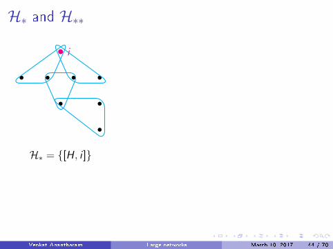
H∗ and H∗∗
i
H∗ = {[H , i ]}
ei
H∗∗ = {[H , e, i ]}
Simple, connected, �nite edges, locally �nite
Venkat Anantharam Large networks March 10, 2017 44 / 70

H∗ and H∗∗
i
H∗ = {[H , i ]}
ei
H∗∗ = {[H , e, i ]}
Simple, connected, �nite edges, locally �nite
Venkat Anantharam Large networks March 10, 2017 44 / 70

H∗ and H∗∗
i
H∗ = {[H , i ]}
ei
H∗∗ = {[H , e, i ]}
Simple, connected, �nite edges, locally �nite
Venkat Anantharam Large networks March 10, 2017 44 / 70
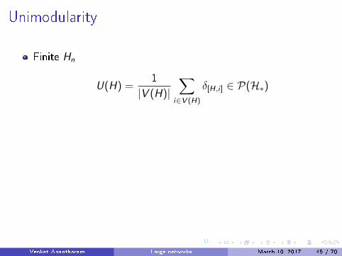
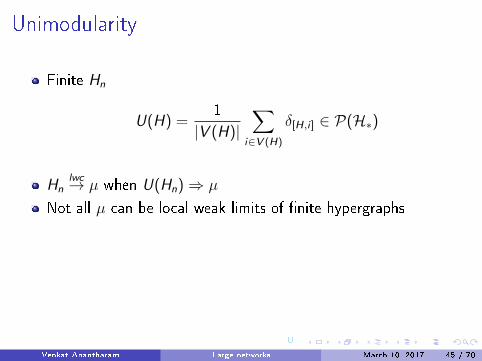
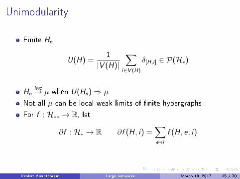
Unimodularity
Finite Hn
U(H) =1
|V (H)|∑
i∈V (H)
δ[H,i ] ∈ P(H∗)
Hnlwc→ µ when U(Hn)⇒ µ
Not all µ can be local weak limits of �nite hypergraphs
For f : H∗∗ → R, let
∂f : H∗ → R ∂f (H , i) =∑e3i
f (H , e, i)
Venkat Anantharam Large networks March 10, 2017 45 / 70
U

Unimodularity
Finite Hn
U(H) =1
|V (H)|∑
i∈V (H)
δ[H,i ] ∈ P(H∗)
Hnlwc→ µ when U(Hn)⇒ µ
Not all µ can be local weak limits of �nite hypergraphs
For f : H∗∗ → R, let
∂f : H∗ → R ∂f (H , i) =∑e3i
f (H , e, i)
Venkat Anantharam Large networks March 10, 2017 45 / 70
U
Unimodularity
Finite Hn
U(H) =1
|V (H)|∑
i∈V (H)
δ[H,i ] ∈ P(H∗)
Hnlwc→ µ when U(Hn)⇒ µ
Not all µ can be local weak limits of �nite hypergraphs
For f : H∗∗ → R, let
∂f : H∗ → R ∂f (H , i) =∑e3i
f (H , e, i)
Venkat Anantharam Large networks March 10, 2017 45 / 70
U
Unimodularity
Finite Hn
U(H) =1
|V (H)|∑
i∈V (H)
δ[H,i ] ∈ P(H∗)
Hnlwc→ µ when U(Hn)⇒ µ
Not all µ can be local weak limits of �nite hypergraphs
For f : H∗∗ → R, let
∂f : H∗ → R ∂f (H , i) =∑e3i
f (H , e, i)
Venkat Anantharam Large networks March 10, 2017 45 / 70
U

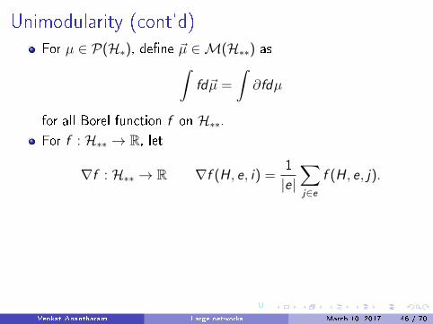
Unimodularity (cont'd)For µ ∈ P(H∗), de�ne ~µ ∈M(H∗∗) as∫
fd~µ =
∫∂fdµ
for all Borel function f on H∗∗.
For f : H∗∗ → R, let
∇f : H∗∗ → R ∇f (H , e, i) =1
|e|∑j∈e
f (H , e, j).
µ ∈ P(H∗) is called unimodular if∫fd~µ =
∫∇fd~µ
If Hnlwc→ µ, µ is unimodular
Venkat Anantharam Large networks March 10, 2017 46 / 70
U
Unimodularity (cont'd)For µ ∈ P(H∗), de�ne ~µ ∈M(H∗∗) as∫
fd~µ =
∫∂fdµ
for all Borel function f on H∗∗.For f : H∗∗ → R, let
∇f : H∗∗ → R ∇f (H , e, i) =1
|e|∑j∈e
f (H , e, j).
µ ∈ P(H∗) is called unimodular if∫fd~µ =
∫∇fd~µ
If Hnlwc→ µ, µ is unimodular
Venkat Anantharam Large networks March 10, 2017 46 / 70
U

Borel Allocations and Balancedness
Θ : H∗∗ → [0, 1] is called a Borel allocation if∑j∈e
Θ(H , e, j) = 1 ∀[H , e, i ] ∈ H∗∗
Θ is balanced w.r.t. µ ∈ P(H∗) if for ~µ�almost all[H , e, i ] ∈ H∗∗
j ∈ e ∂Θ(H , i) > ∂Θ(H , j) ⇒ Θ(H , e, i) = 0.
Venkat Anantharam Large networks March 10, 2017 47 / 70

Borel Allocations and Balancedness
Θ : H∗∗ → [0, 1] is called a Borel allocation if∑j∈e
Θ(H , e, j) = 1 ∀[H , e, i ] ∈ H∗∗
Θ is balanced w.r.t. µ ∈ P(H∗) if for ~µ�almost all[H , e, i ] ∈ H∗∗
j ∈ e ∂Θ(H , i) > ∂Θ(H , j) ⇒ Θ(H , e, i) = 0.
Venkat Anantharam Large networks March 10, 2017 47 / 70

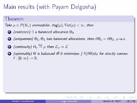
Main results (with Payam Delgosha)
TheoremTake µ ∈ P(H∗) unimodular, deg(µ),Var(µ) <∞, then
1 (existence) ∃ a balanced allocation Θ0
2 (uniqueness) Θ1,Θ2 two balanced allocations, then ∂Θ1 = ∂Θ2, µ�a.s.
3 (continuity) Hnlwc→ µ then Ln ⇒ L
4 (optimality) Θ is balanced i� it minimizes∫f (∂Θ)dµ for strictly convex
f : [0,∞)→ R.
5 (variational characterization) t ∈ R and Θ balanced, then∫(∂Θ− t)+dµ = max
f∈H∗Borel→ [0,1]
∫f̃mind~µ− t
∫fdµ
where f̃min(H, e, i) = 1
|e| minj∈e f (H, j).
Venkat Anantharam Large networks March 10, 2017 48 / 70
Hajek CE VC

Response Function
i
......
↓ x
ρT ,i(x) = total load at i with baseload x
x
ρ(x)
i
......
↓ ?t
ρ−1T ,i(t): the amount of extra loadso that the total load becomes t
Venkat Anantharam Large networks March 10, 2017 49 / 70

Response Function
i
......
↓ x ρT ,i(x) = total load at i with baseload x
x
ρ(x)
i
......
↓ ?t
ρ−1T ,i(t): the amount of extra loadso that the total load becomes t
Venkat Anantharam Large networks March 10, 2017 49 / 70

Response Function
i
......
↓ x ρT ,i(x) = total load at i with baseload x
x
ρ(x)
i
......
↓ ?t
ρ−1T ,i(t): the amount of extra loadso that the total load becomes t
Venkat Anantharam Large networks March 10, 2017 49 / 70

Response Function
i
......
↓ x ρT ,i(x) = total load at i with baseload x
x
ρ(x)
i
......
↓ ?t
ρ−1T ,i(t): the amount of extra loadso that the total load becomes t
Venkat Anantharam Large networks March 10, 2017 49 / 70

Response Function
i
......
↓ x ρT ,i(x) = total load at i with baseload x
x
ρ(x)
i
......
↓ ?t
ρ−1T ,i(t): the amount of extra loadso that the total load becomes t
Venkat Anantharam Large networks March 10, 2017 49 / 70

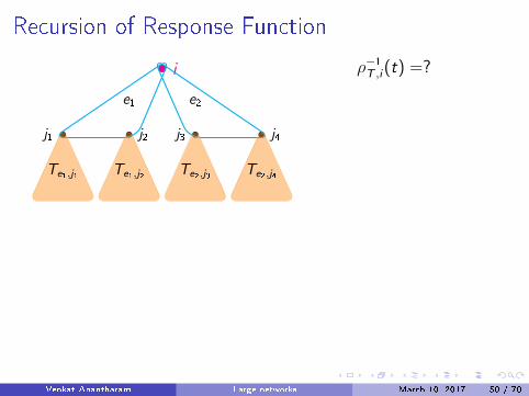
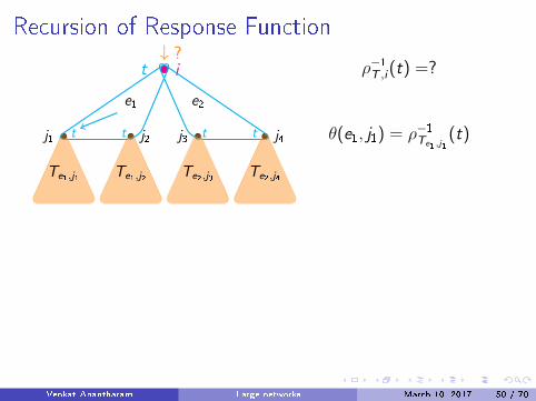
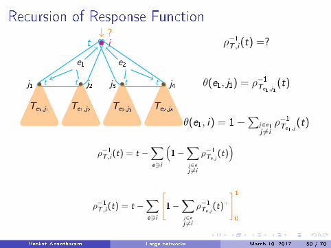
Recursion of Response Function
i
j2j1 j3 j4
e1 e2
Te1,j2Te1,j1 Te2,j3 Te2,j4
ρ−1T ,i(t) =?↓ ?
t
t t tt θ(e1, j1) = ρ−1Te1,j1(t)
θ(e1, i) = 1−∑
j∈e1j 6=i
ρ−1Te1,j(t)
ρ−1T ,i (t) = t −∑e3i
(1−
∑j∈ej 6=i
ρ−1Te,j(t))
ρ−1T ,i (t) = t −∑e3i
[1−
∑j∈ej 6=i
ρ−1Te,j(t)+
]10
Venkat Anantharam Large networks March 10, 2017 50 / 70
Recursion of Response Function
i
j2j1 j3 j4
e1 e2
Te1,j2Te1,j1 Te2,j3 Te2,j4
ρ−1T ,i(t) =?
↓ ?t
t t tt θ(e1, j1) = ρ−1Te1,j1(t)
θ(e1, i) = 1−∑
j∈e1j 6=i
ρ−1Te1,j(t)
ρ−1T ,i (t) = t −∑e3i
(1−
∑j∈ej 6=i
ρ−1Te,j(t))
ρ−1T ,i (t) = t −∑e3i
[1−
∑j∈ej 6=i
ρ−1Te,j(t)+
]10
Venkat Anantharam Large networks March 10, 2017 50 / 70

Recursion of Response Function
i
j2j1 j3 j4
e1 e2
Te1,j2Te1,j1 Te2,j3 Te2,j4
ρ−1T ,i(t) =?↓ ?
t
t t tt θ(e1, j1) = ρ−1Te1,j1(t)
θ(e1, i) = 1−∑
j∈e1j 6=i
ρ−1Te1,j(t)
ρ−1T ,i (t) = t −∑e3i
(1−
∑j∈ej 6=i
ρ−1Te,j(t))
ρ−1T ,i (t) = t −∑e3i
[1−
∑j∈ej 6=i
ρ−1Te,j(t)+
]10
Venkat Anantharam Large networks March 10, 2017 50 / 70

Recursion of Response Function
i
j2j1 j3 j4
e1 e2
Te1,j2Te1,j1 Te2,j3 Te2,j4
ρ−1T ,i(t) =?↓ ?
t
t t tt
θ(e1, j1) = ρ−1Te1,j1(t)
θ(e1, i) = 1−∑
j∈e1j 6=i
ρ−1Te1,j(t)
ρ−1T ,i (t) = t −∑e3i
(1−
∑j∈ej 6=i
ρ−1Te,j(t))
ρ−1T ,i (t) = t −∑e3i
[1−
∑j∈ej 6=i
ρ−1Te,j(t)+
]10
Venkat Anantharam Large networks March 10, 2017 50 / 70
Recursion of Response Function
i
j2j1 j3 j4
e1 e2
Te1,j2Te1,j1 Te2,j3 Te2,j4
ρ−1T ,i(t) =?↓ ?
t
t t tt θ(e1, j1) = ρ−1Te1,j1(t)
θ(e1, i) = 1−∑
j∈e1j 6=i
ρ−1Te1,j(t)
ρ−1T ,i (t) = t −∑e3i
(1−
∑j∈ej 6=i
ρ−1Te,j(t))
ρ−1T ,i (t) = t −∑e3i
[1−
∑j∈ej 6=i
ρ−1Te,j(t)+
]10
Venkat Anantharam Large networks March 10, 2017 50 / 70

Recursion of Response Function
i
j2j1 j3 j4
e1 e2
Te1,j2Te1,j1 Te2,j3 Te2,j4
ρ−1T ,i(t) =?↓ ?
t
t t tt θ(e1, j1) = ρ−1Te1,j1(t)
θ(e1, i) = 1−∑
j∈e1j 6=i
ρ−1Te1,j(t)
ρ−1T ,i (t) = t −∑e3i
(1−
∑j∈ej 6=i
ρ−1Te,j(t))
ρ−1T ,i (t) = t −∑e3i
[1−
∑j∈ej 6=i
ρ−1Te,j(t)+
]10
Venkat Anantharam Large networks March 10, 2017 50 / 70

Unimodular Galton Watson Hypertrees
All the hyperedges have size c (say 3)
distribution P on non�negative integers
P
P̂
......
......
......
P̂k = (k+1)Pk+1
E[P]
UGWTc(P) ∈ P(H∗) is unimodular
Venkat Anantharam Large networks March 10, 2017 51 / 70

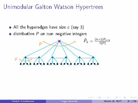
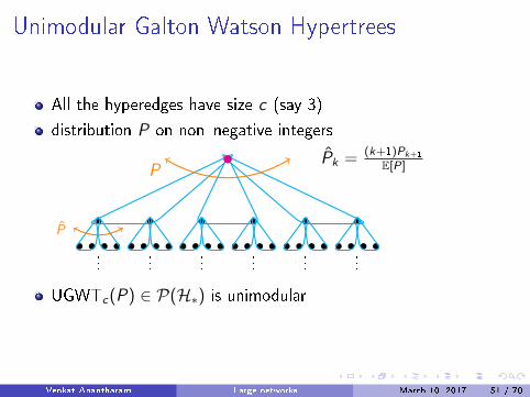
Unimodular Galton Watson Hypertrees
All the hyperedges have size c (say 3)
distribution P on non�negative integers
P
P̂
......
......
......
P̂k = (k+1)Pk+1
E[P]
UGWTc(P) ∈ P(H∗) is unimodular
Venkat Anantharam Large networks March 10, 2017 51 / 70
Unimodular Galton Watson Hypertrees
All the hyperedges have size c (say 3)
distribution P on non�negative integers
P
P̂
......
......
......
P̂k = (k+1)Pk+1
E[P]
UGWTc(P) ∈ P(H∗) is unimodular
Venkat Anantharam Large networks March 10, 2017 51 / 70

Unimodular Galton Watson Hypertrees
All the hyperedges have size c (say 3)
distribution P on non�negative integers
P
P̂
......
......
......
P̂k = (k+1)Pk+1
E[P]
UGWTc(P) ∈ P(H∗) is unimodular
Venkat Anantharam Large networks March 10, 2017 51 / 70
Unimodular Galton Watson Hypertrees
All the hyperedges have size c (say 3)
distribution P on non�negative integers
P
P̂
......
......
......
P̂k = (k+1)Pk+1
E[P]
UGWTc(P) ∈ P(H∗) is unimodular
Venkat Anantharam Large networks March 10, 2017 51 / 70

Unimodular Galton Watson Hypertrees
All the hyperedges have size c (say 3)
distribution P on non�negative integers
P
P̂
......
......
......
P̂k = (k+1)Pk+1
E[P]
UGWTc(P) ∈ P(H∗) is unimodular
Venkat Anantharam Large networks March 10, 2017 51 / 70
Unimodular Galton Watson Hypertrees
All the hyperedges have size c (say 3)
distribution P on non�negative integers
P
P̂
......
......
......
P̂k = (k+1)Pk+1
E[P]
UGWTc(P) ∈ P(H∗) is unimodular
Venkat Anantharam Large networks March 10, 2017 51 / 70
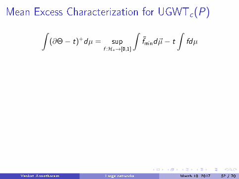
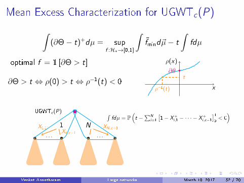
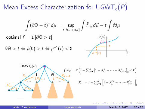
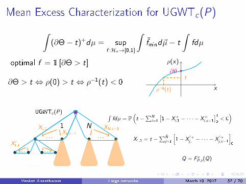
Mean Excess Characterization for UGWTc(P)
∫(∂Θ− t)+dµ = sup
f :H∗→[0,1]
∫f̃mind~µ− t
∫fdµ
optimal f = 1 [∂Θ > t]
∂Θ > t ⇔ ρ(0) > t ⇔ ρ−1(t) < 0x
ρ(x)
∂θ
ρ−1(t)
t
UGWTc(P)
. . . . . .
1 N
∫fdµ = P
(t −
∑Ni=1
[1− X+
i ,1 − · · · − X+i ,c−1
]10< 0)
X1,1X1,c−1
XN,c−1
. . . . . .X ′1,1
X1,1 = t −∑N̂
j=1
[1− X
′+j ,1 − · · · − X
′+j ,c−1
]10
Q = F cP,t(Q)
Venkat Anantharam Large networks March 10, 2017 52 / 70

Mean Excess Characterization for UGWTc(P)
(cont'd)
Theorem
Assume P is a distribution on nonnegative integers with �nitevariance and µ = UGWTc(P). Then, we have∫
(∂Θ− t)+dµ = maxQ:F c
P,t(Q)=Q
E [N]
cP(X+1
+ · · ·+ X+c < 1
)− tP (Y1 + · · ·+ YN > t) ,
where N has distribution P , Xi 's are independent and have
distribution Q and Yi 's are independent and each have distribution of
[1− (X+1 + · · ·+ X+
c−1)]10 where Xi 's are i.i.d. from Q.
Venkat Anantharam Large networks March 10, 2017 53 / 70

Outline
1 A resource allocation problem studied by Hajek
2 Load balancing on graphs
3 The framework of local weak convergence
4 Load balancing on hypergraphs
5 Graph indexed data
6 Universal compression of graphical data
Venkat Anantharam Large networks March 10, 2017 54 / 70
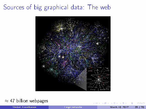
Sources of big graphical data: The web
≈ 47 billion webpagesVenkat Anantharam Large networks March 10, 2017 55 / 70

Sources of big graphical data: Social networks
≈ 1.8 billion active users on Facebook
Venkat Anantharam Large networks March 10, 2017 56 / 70
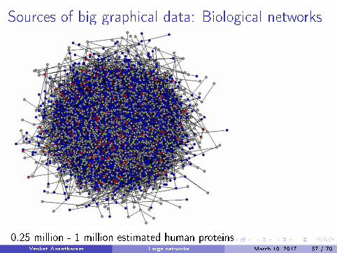
Sources of big graphical data: Biological networks
0.25 million - 1 million estimated human proteinsVenkat Anantharam Large networks March 10, 2017 57 / 70
Universal compression of marked graphical data
We want to compress down to the �entropy" of the data.
Universality means that the scheme should work irrespective ofthe underlying �statistics" of the data.
Ideally, the compressed representation should enable analysis andquerying in the compressed form
The local weak limit theory allows one to precisely formulate theuniversal compression problem and to provide a solution.
Venkat Anantharam Large networks March 10, 2017 58 / 70

The BC entropy: counting typical graphs
Ξ: edge marks, Θ: vertex marks, both �nite
G(n)mn,un : set of graphs on n vertices with mn(x) many edges with
mark x ∈ Ξ and un(t) many vertices with mark t ∈ Θ.
G(n)mn,un(µ, ε) = {G ∈ G(n)
mn,un : U(G ) ∈ B(µ, ε)}.For µ ∈ P(G∗) and x ∈ Ξ, degx(µ): expected number of edgesconnected to the root with mark x ,
t ∈ Θ, Πt(µ): probability of root having mark t.
Venkat Anantharam Large networks March 10, 2017 59 / 70
The BC entropy: counting typical graphs
Fix sequences mn,un such that mn(x)/n→ degx(µ)/2 andun(t)/n→ Πt(µ) for all x ∈ Ξ, t ∈ Θ.
log |G(n)mn,un | = ‖mn‖1 log n + cn + o(n) where
‖mn‖1 =∑
x∈Ξmn(x).
Σ(µ) := limε↓0
lim supn→∞
log |G (n)mn,un(µ, ε)| − ‖mn‖1 log n
n
Σ(µ) := limε↓0
lim infn→∞
log |G (n)mn,un(µ, ε)| − ‖mn‖1 log n
n
If they are equal, de�ne the common value as Σ(µ)(Generalizing work of Bordenave and Caputo)
Venkat Anantharam Large networks March 10, 2017 60 / 70

Outline
1 A resource allocation problem studied by Hajek
2 Load balancing on graphs
3 The framework of local weak convergence
4 Load balancing on hypergraphs
5 Graph indexed data
6 Universal compression of graphical data
Venkat Anantharam Large networks March 10, 2017 61 / 70

Our target for the graph regime
Goal: design fn : Gn → {0, 1}∗ and gn : {0, 1}∗ → Gngn ◦ fn = Id
µ ∈ P(G∗) a process
Target: typical graphs
Optimal if Gnlwc→ µ
lim supn→∞
l(fn(Gn))−mn log n
n≤ Σ(µ),
where mn is the total number of edges in Gn.
Venkat Anantharam Large networks March 10, 2017 62 / 70
A First Step Coding Scheme : Example
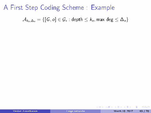
Akn,∆n = {[G , o] ∈ G∗ : depth ≤ kn,max deg ≤ ∆n}
n = 4, kn = 1
1 2
4 3
∆n = 2
0 0 0 0 0 0 0 0 0 0 04
Wn := the set of graphs with the same sequence
1 2
4 3
1 2
4 3
1 2
4 3
1 2
4 3
1 2
4 3
1 2
4 3
Venkat Anantharam Large networks March 10, 2017 63 / 70

A First Step Coding Scheme : Example
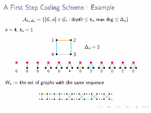
Akn,∆n = {[G , o] ∈ G∗ : depth ≤ kn,max deg ≤ ∆n}
n = 4, kn = 1
1 2
4 3
∆n = 2
0 0 0 0 0 0 0 0 0 0 04
Wn := the set of graphs with the same sequence
1 2
4 3
1 2
4 3
1 2
4 3
1 2
4 3
1 2
4 3
1 2
4 3
Venkat Anantharam Large networks March 10, 2017 63 / 70

A First Step Coding Scheme : Example
Akn,∆n = {[G , o] ∈ G∗ : depth ≤ kn,max deg ≤ ∆n}
n = 4, kn = 1
1 2
4 3
∆n = 2
0 0 0 0 0 0 0 0 0 0 04
Wn := the set of graphs with the same sequence
1 2
4 3
1 2
4 3
1 2
4 3
1 2
4 3
1 2
4 3
1 2
4 3
Venkat Anantharam Large networks March 10, 2017 63 / 70

A First Step Coding Scheme : Example
Akn,∆n = {[G , o] ∈ G∗ : depth ≤ kn,max deg ≤ ∆n}
n = 4, kn = 1
1 2
4 3
∆n = 2
0 0 0 0 0 0 0 0 0 0 04
Wn := the set of graphs with the same sequence
1 2
4 3
1 2
4 3
1 2
4 3
1 2
4 3
1 2
4 3
1 2
4 3
Venkat Anantharam Large networks March 10, 2017 63 / 70

A First Step Coding Scheme : Example
Akn,∆n = {[G , o] ∈ G∗ : depth ≤ kn,max deg ≤ ∆n}
n = 4, kn = 1
1 2
4 3
∆n = 2
0 0 0 0 0 0 0 0 0 0 04
Wn := the set of graphs with the same sequence
1 2
4 3
1 2
4 3
1 2
4 3
1 2
4 3
1 2
4 3
1 2
4 3
Venkat Anantharam Large networks March 10, 2017 63 / 70
A First Step Coding Scheme : Example
Akn,∆n = {[G , o] ∈ G∗ : depth ≤ kn,max deg ≤ ∆n}
n = 4, kn = 1
1 2
4 3
∆n = 2
0 0 0 0 0 0 0 0 0 0 04
Wn := the set of graphs with the same sequence
1 2
4 3
1 2
4 3
1 2
4 3
1 2
4 3
1 2
4 3
1 2
4 3
Venkat Anantharam Large networks March 10, 2017 63 / 70

A First Step Coding Scheme : Example
Akn,∆n = {[G , o] ∈ G∗ : depth ≤ kn,max deg ≤ ∆n}
n = 4, kn = 1
1 2
4 3
∆n = 2
0 0 0 0 0 0 0 0 0 0 04
Wn := the set of graphs with the same sequence
1 2
4 3
1 2
4 3
1 2
4 3
1 2
4 3
1 2
4 3
1 2
4 3
Venkat Anantharam Large networks March 10, 2017 63 / 70
Analysis Outline
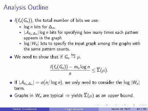
l(fn(Gn)), the total number of bits we use:I log n bits for ∆n,I |Akn,∆n | log n bits for specifying how many times each pattern
appears in the graphI log |Wn| bits to specify the input graph among the graphs with
the same pattern counts.
We need to show that if Gnlwc→ µ,
l(fn(Gn))−mn log n
n≤ Σ(µ).
If |Akn,∆n | = o(n/ log n), we only need to consider the log |Wn|term.
Graphs in Wn are typical ⇒ yields Σ(µ) as an upper bound.
Venkat Anantharam Large networks March 10, 2017 64 / 70

First step algorithm: Main Result
Proposition
If parameters kn and ∆n are such that |Akn,∆n | = o( nlog n
) and
kn →∞ as n→∞, for any sequence Gn with maximum degree no
more than ∆n and local weak limit µ ∈ P(G∗) such that Σ(µ) > −∞we have
lim supn→∞
l(fn(Gn))−mn log n
n≤ Σ(µ), (1)
where mn is the number of edges in Gn.
Venkat Anantharam Large networks March 10, 2017 65 / 70

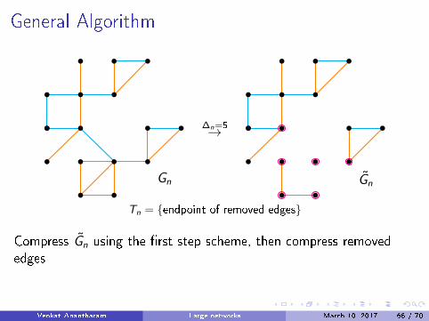
General Algorithm
Gn
∆n=5→
G̃n
Tn = {endpoint of removed edges}
Compress G̃n using the �rst step scheme, then compress removededges ∆n = log log n kn =
√log log n
|Tn|/n→ 0 |Akn,∆n | = o(n/ log n) Gnlwc→ µ⇒ G̃n
lwc→ µ
Venkat Anantharam Large networks March 10, 2017 66 / 70

General Algorithm
Gn
∆n=5→
G̃n
Tn = {endpoint of removed edges}
Compress G̃n using the �rst step scheme, then compress removededges ∆n = log log n kn =
√log log n
|Tn|/n→ 0 |Akn,∆n | = o(n/ log n) Gnlwc→ µ⇒ G̃n
lwc→ µ
Venkat Anantharam Large networks March 10, 2017 66 / 70

General Algorithm
Gn
∆n=5→
G̃n
Tn = {endpoint of removed edges}
Compress G̃n using the �rst step scheme, then compress removededges ∆n = log log n kn =
√log log n
|Tn|/n→ 0 |Akn,∆n | = o(n/ log n) Gnlwc→ µ⇒ G̃n
lwc→ µ
Venkat Anantharam Large networks March 10, 2017 66 / 70

General Algorithm
Gn
∆n=5→
G̃n
Tn = {endpoint of removed edges}
Compress G̃n using the �rst step scheme, then compress removededges ∆n = log log n kn =
√log log n
|Tn|/n→ 0 |Akn,∆n | = o(n/ log n) Gnlwc→ µ⇒ G̃n
lwc→ µ
Venkat Anantharam Large networks March 10, 2017 66 / 70
General Algorithm
Gn
∆n=5→
G̃n
Tn = {endpoint of removed edges}
Compress G̃n using the �rst step scheme, then compress removededges
∆n = log log n kn =√
log log n
|Tn|/n→ 0 |Akn,∆n | = o(n/ log n) Gnlwc→ µ⇒ G̃n
lwc→ µ
Venkat Anantharam Large networks March 10, 2017 66 / 70

General Algorithm
Gn
∆n=5→
G̃n
Tn = {endpoint of removed edges}
Compress G̃n using the �rst step scheme, then compress removededges ∆n = log log n kn =
√log log n
|Tn|/n→ 0 |Akn,∆n | = o(n/ log n) Gnlwc→ µ⇒ G̃n
lwc→ µ
Venkat Anantharam Large networks March 10, 2017 66 / 70

General Algorithm
Gn
∆n=5→
G̃n
Tn = {endpoint of removed edges}
Compress G̃n using the �rst step scheme, then compress removededges ∆n = log log n kn =
√log log n
|Tn|/n→ 0 |Akn,∆n | = o(n/ log n) Gnlwc→ µ⇒ G̃n
lwc→ µ
Venkat Anantharam Large networks March 10, 2017 66 / 70

Result: Achievability
Theorem
Assume µ ∈ G∗ with degx(µ) <∞ for all x and Σ(µ) > −∞. If Gn
is a sequence of marked graphs with local weak limit µ, we have
lim supn→∞
l(fn(Gn))−mn log n
n≤ Σ(µ),
where mn is the number of edges in Gn.
Venkat Anantharam Large networks March 10, 2017 67 / 70
Result: Converse
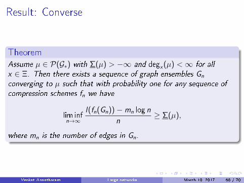
Theorem
Assume µ ∈ P(G∗) with Σ(µ) > −∞ and degx(µ) <∞ for all
x ∈ Ξ. Then there exists a sequence of graph ensembles Gn
converging to µ such that with probability one for any sequence of
compression schemes fn we have
lim infn→∞
l(fn(Gn))−mn log n
n≥ Σ(µ),
where mn is the number of edges in Gn.
Venkat Anantharam Large networks March 10, 2017 68 / 70
Concuding remarks
Just like a stochastic process is a model for the statistics of along string of data, a local weak limit of marked graphs is amodel for the statistics of data that lives on large graphs.
This provides a methodology to address networking problemsand data centric problems arising in networks that parallels howstochastic processs are used in the study of time series.
This was illustrated with two kinds of applications: resourceallocation in graphs and hypergraphs, and universal losslessscompression of graph-structured data.
A world of other applications awaits.
Venkat Anantharam Large networks March 10, 2017 69 / 70

The End
Venkat Anantharam Large networks March 10, 2017 70 / 70


![arXiv:1804.07902v1 [math.AP] 21 Apr 2018 · 2018. 11. 9. · developed in [FPR09, RR15]. When taking the time discrete-to-continuous limit, we first pass to the limit in the weak](https://img.pdfslide.us/doc/110x75/60c2d03653c92a7c7f3a2bd6/arxiv180407902v1-mathap-21-apr-2018-2018-11-9-developed-in-fpr09-rr15.jpg)