Embed Size (px)
Citation preview
Study on Stationkeeping for Halo Orbits at EL1: Dynamics Modeling
and Controller Designing
By Ming XU and Shijie XU
Department of Aerospace Engineering, School of Astronautics, Beihang University, Beijing, China
(Received March 7th, 2011)
This paper deals with the stationkeeping control for halo orbits at EL1 in the Sun-Earth/Moon system, and proposes
an effective adaptive robust controller for the unknown spacecraft mass and perturbation boundaries. The controller has
to deal with two divergence sources: one is the instability of the halo orbit, and the other is the perturbation imposed by
the natural model onto the nominal model. The former source is displayed by the Floquet multiplier from the Poincare
mapping. However, the latter is revealed by the difference of Hamiltonian functions between the nominal reference
model, the circular restricted three-body problem (CR3BP) and the natural simulation model, the spatial bicircular
model (SBCM). Firstly, the algorithm of backstepping control theory is employed to generate the initial controller in
the nominal reference model of CR3BP. Some improvements are then implemented for the estimations of the unknown
parameters as the perturbation boundaries and the spacecraft mass, which may cause the failure of the initial unimproved
controller in stationkeeping. The controller proves to be effective in terms of adaptive robust estimation and asymptotic
stability from Lyapunov’s stability theory. Furthermore, further improvements of the triggers for the on/off schedule are
proposed to remedy the weakness in the capability of estimating for excessively long (infinite) time required to converge.
Finally, the controller developed in this paper is implemented in the natural simulation model of SBCM to evaluate its
performance. In the numerical simulation, the mass and perturbation boundaries will converge only after approximately
three iterations. The deviation of the estimating mass is 1 kg from its true mass, but 55 kg for the unimproved controller.
The total velocity increment over five years is only 126m/s, which is equivalent to the fuel consumption of 3.8 kg for the
Hall thrust engine carried by SMART-1.
Key Words: Libration Point, Halo Orbit, Stationkeeping, Robust Adaptive Strategy, Backstepping Design
1. Introduction
Since the success of ISEE-3 in 1978, libration points and
halo orbits have drawn much attention from the astronauti-
cal society all over the world.1) So far there have been seven
missions involving in the libration point or halo orbits for
solar observation, early warning systems for solar wind or
deep-space telescopes, such as ISEE-3 (1978), Wind
(1994), SOHO (1995), ACE (1997), Genesis (2001), MAP
(2001) and Planck (2009). Of these, the last two missions
were at EL2 and the others at EL1.
It is well known that halo orbits near the collinear libra-
tion points are unstable,2) thus the stationkeeping control
is necessary to keep the spacecraft near the nominal trajec-
tory. The method of achieving this has been a common focus
of research since the first mission for the libration point was
implemented. Up to now, some control strategies have been
proposed by employing different control theories, and they
can be classified into two modes: the target and Floquet
modes.1) The former keeps the spacecraft flying on the nom-
inal trajectory with frequent controls. The latter, however,
locates the spacecraft on the invariant manifolds of the halo
orbit with the controller compensating for the unstable
manifolds in order to avoid divergence. The Floquet mode
was developed by Simo et al.3) from the view of dynamical
system theory. It is more complicated in terms of controller
design but results in less fuel consumption than the target
mode. Despite this higher fuel consumption, the target mode
has more potential applications from modern control theo-
ries. Farquhar2) and Breakwell et al.4) are pioneers in
employing the feedback control in this opening problem.
Howell and Pernicka5) designed the linear controller for
the stationkeeping on halo orbits from the balanced view
of control precision and fuel assumption. Giamberardino
and Monaco6) designed a nonlinear controller to track the
halo orbit asymptotically based on a linear model. Cielaszyk
and Wie7) used a numerical method developed from LQR to
generate and maintain the halo orbit. Kulkarni and Camp-
bell8) applied the H1 theory to the stationkeeping for halo
orbits, and then applied the development strategy to main-
tain the formation of several spacecrafts flying around halo
orbits. Wong and Kaplia9) developed the adaptive control
strategy for this question and proved the stability of the con-
troller designed. Xu and Xu10) achieved the linear periodic
strategy for stationkeeping control based on the periodicity
of halo orbits.
For long flights in deep space far from the Earth, space-
craft should have the capabilities to deal with uncertainties
such as mismodeled accelerations in the N-body gravita-
tional fields (with unknown upper-boundary) and unknown
parameters of the spacecraft (such as mass and moment of� 2012 The Japan Society for Aeronautical and Space Sciences
Trans. Japan Soc. Aero. Space Sci.
Vol. 55, No. 5, pp. 274–285, 2012
inertia). There are several studies on estimating the inertia
moment associated with the attitude control.11–13) However,
there are no papers discussing the stationkeeping control for
halo orbits with the unknown parameters or perturbations.
Therefore, we will deal with the stationkeeping for the halo
orbit at the libration point EL1 in the Sun-Earth/Moon sys-
tem, and design a robustly adaptive controller associated
with estimating the spacecraft mass and the upper-boundary
of the disturbances.
To understand the stability of nominal trajectory gener-
ated from the reference model of the circular restricted three
body problem (CR3BP), the Floquet multiplier is calculated
from the Poincare mapping to indicate the instability of halo
orbits, which needs to be compensated by the controller. To
understand the unknown perturbations between the nominal
reference model and natural model, the difference of Ham-
iltonian functions is derived to check whether the lunar
gravitational perturbation is small enough that the reference
model can be considered as a reasonable approximation of
the natural simulation model from the view of the Hamilto-
nian dynamical system. So the controller developed in this
paper has to deal with two divergence sources: one is the
perturbation between nominal and natural models, and the
other is the instability of the halo orbit caused by its large
Floquet multiplier.
The controller is designed based on the nominal reference
model of the CR3BP, and is then implemented in the natural
simulation model of the spatial bicircular model (SBCM) to
evaluate its performance. The algorithm of backstepping
control is employed to generate the initial controller. How-
ever, the controller requires some improvements for the
estimations of the unknown parameters such as the bound-
ary of perturbations from the nominal and natural models
and the mass of spacecraft, which may cause the failure of
the unimproved controller. The improvements prove to be
effective in terms of adaptive robust estimation and asymp-
totic stability from Lyapunov’s stability theory. However,
the controller is still weak in dealing with the estimation re-
quired to converge for excessively long (infinite) time. So
further improvements of the on/off schedule for the trigger
are proposed.
2. Dynamical Modeling
2.1. Unit normalization and coordinate system defini-
tion
The equations derived in this paper can be normalized by
means of the characteristic length, time and mass, as below:
½L� ¼ RS-E/M; average distance between the Sun and the barycenter of the Earth and Moon
½M� ¼ mS þ mE/M; total mass in the Sun-Earth/Moon system
½T� ¼ R3S-E/M=GðmS þ mE/MÞ
� �1=28><>:
where mS and mE/M are the mass of the Sun and Earth/
Moon, respectively, and G is the universal gravitation con-
stant.
Three different coordinates are referred to in this paper as:
the syzygy frame in the Sun-Earth/Moon system (SS-E/M),
the inertial frame in the Sun-Earth/Moon system (IS-E/M),
and the syzygy frame in the Earth/Moon system (SE/M).
The reason for introducing the syzygy frames, such as
SS-E/M and SE/M, is so that they can be used to reduce the
computational work in Kepler circular motions in the Sun-
Earth/Moon and Earth/Moon systems, and to greatly im-
prove the computing efficiency for long simulations.
The IS-E/M frame with its components of ðX; Y ; ZÞ has thefollowing features: the origin O is fixed at the barycenter of
the Sun-Earth/Moon system; the Z axis is perpendicular to
the ecliptic plane and along the revolution axis of the Earth/
Moon system; the X axis, which follows an inertial direction
in the system, is along the intersection of the ecliptic and the
lunar plane; and the Y axis is determined by the right-hand-
side rule.
The SS-E/M frame with its components of ðx; y; zÞ has thefollowing features: the origin O is fixed at the barycenter of
the Sun-Earth/Moon system; the z axis is perpendicular to
the ecliptic orbital plane; the x axis points from the Sun to
OE/M; and the y axis is determined by the right-hand-side
rule. The mass ratio of the Earth and Moon subject to the
total mass of the Sun-Earth/Moon system can be defined
as �S ¼ mE/M=ðmS þ mE/MÞ. Then the coordinate compo-
nents of the Sun and OE/M in the syzygy frame can then
be solved from the normalization as ½��S 0 0�T and
½1� �S 0 0�T, respectively, to implement the reduction
in computing the Kepler circular motion introduced by the
definition of the syzygy frame.
The SE/M frame with its components ð�; �; �Þ has the fol-lowing features: the origin O is set at the barycenter of the
Earth/Moon system; the � axis is perpendicular to the lunar
plane and along the revolution axis of the Moon; the � axis
points from the Earth to the Moon; and the � axis is deter-
mined by the right-hand-side rule. Thus, the position vectors
rE and rM of the Earth and Moon in SE/M can be expressed
simply as
rE ¼RE-M
RS-E/M
� �mM
mE þ mM
0 0
� �Tand
rM ¼RE-M
RS-E/M
�mE
mE þ mM
0 0
� �T;
where mE and mM are the mass of Earth and Moon, respec-
tively, and the relationship exists whereby mE þ mM ¼ �S,
and RE-M is the averaging distance from Earth to Moon. Fur-
thermore, the identical equation can be achieved from the
definition of the SE/M frame and Newton’s gravitational
equation as mE � rE þ mM � rM ¼ 0.
Sep. 2012 M. XU and S. XU: Study on Stationkeeping for Halo Orbits at EL1 275
2.2. CR3BP
2.2.1. CR3BP assumption
The astrodynamics in the gravitational field of the Sun-
Earth/Moon system has a famous simplified form in celes-
tial mechanics referred as the circular restricted three body
problem (CR3BP), which is an open unsolved problem first
proposed by Newton.14) The assumptions for the simplified
model in the Sun-Earth/Moon system are summarized as:
a) The Earth and Moon act as one whole gravitational
point with its position located in their centroid OE/M;
b) The gravitational point stays circumsolar in the
ecliptic plane with relatively small eccentricity (e � 0:01)
ignored.
2.2.2. Dynamics in CR3BP
The CR3BP has different dynamics equations in the dif-
ferent frames referred in section 2.1. The dynamics in
SS-E/M, however, have a more simplified form than in the
others and reduces the computing work in the Kepler circu-
lar motion introduced by the definition of the syzygy frame.
The position vector of the spacecraft in the syzygy frame
is denoted as R ¼ ½x y z�T, and the generalized momen-
tum P ¼ ½px py pz�T is defined as
px ¼ _xx� y
py ¼ _yyþ x
pz ¼ _zz:
8<: ð1Þ
Then, the Hamiltonian function is
H0 ¼1
2p2x þ p2y þ p2z
� �� xpy þ ypx �
1� �S
rS�
�S
rE-Mð2Þ
where
rS ¼ffiffiffiffiffiffiffiffiffiffiffiffiffiffiffiffiffiffiffiffiffiffiffiffiffiffiffiffiffiffiffiffiffiffiffiffiffiffiffiðxþ �SÞ2 þ y2 þ z2
q
is the distance between the spacecraft and the Sun, and
rE-M ¼ffiffiffiffiffiffiffiffiffiffiffiffiffiffiffiffiffiffiffiffiffiffiffiffiffiffiffiffiffiffiffiffiffiffiffiffiffiffiffiffiffiffiffiffiffiffiffiðxþ �S � 1Þ2 þ y2 þ z2
qis the distance between the spacecraft and OE/M. The
Hamiltonian dynamics in the model of CR3BP can be ex-
pressed as:
_RR ¼@H0
@P
_PP ¼ �@H0
@R:
8>><>>: ð3Þ
Expanding the above equation yields the Hamiltonian
dynamics in their components as
€xx
€yy
€zz
264
375 ¼ �2
� _yy
_xx
0
264
375þ
x
y
0
264
375�
1� �S
r3S½Rþ �Se1�
��S
r3E-M½R� ð1� �SÞe1� ð4Þ
where e1 ¼ ½1 0 0�T is the unit vector along the x axis.
Though the Hamiltonian dynamics in the model of
CR3BP are non-integrable, Eq. (4) has five special solu-
tions, named as libration points (or Lagrange points, denoted
as Li, i ¼ 1; � � � ; 5), of which L1, L2 and L3 are collinear
points (with the second and third components of yL ¼ 0,
zL ¼ 0) and L4 and L5 are triangular points (with the third
components of zL ¼ 0). The locations of the libration
points can be achieved by solving the algebraic equations
generated by setting the right sides of Eq. (4) to zero. This
paper concentrates more on the point of EL1 with its first
component as
xL ¼ ð1� �SÞ
���S
3
1=3
1þ1
3
��S
3
1=3
�1
9
��S
3
2=3
þ � � �
" #
� 0:98999093: ð5Þ
2.3. SBCM
2.3.1. SBCM assumption
The SBCM originates from the planar BCM (PBCM)
introduced by Andreu15) and Koon et al.16) in the planar
analysis on lunar low-energy transfer, which is a reasonable
approximation of the CR3BP. However, the SBCM shows
significant improvements in the inclination between the
ecliptic and lunar planes, which has an important application
in spatial analysis on astrodynamics.17,18) Compared with
the CR3BP, the SBCM has the following assumptions:
a) The Earth and Moon act as different simple gravita-
tional points, and move round their centroid in Kepler circu-
lar motions with their eccentricity ignored;
b) The centroid of the Earth/Moon system stays cir-
cumsolar in the ecliptic plane with the eccentricity ignored;
c) The inclination of the lunar plane relative to the
ecliptic plane is considered as the average angle of 5�90.
The SBCM shows significant improvements in terms of
the extra gravitational force implemented by the Moon
and the inclination between the ecliptic and lunar planes,
which are neglected by the CR3BP. The difference of the
two models’ Hamiltonian functions will be checked in sec-
tion 2.3.4, and whether lunar gravity is so small that the
CR3BP can be considered as a reasonable approximation
of the SBCM from the view of the Hamiltonian dynamical
system will be stated.
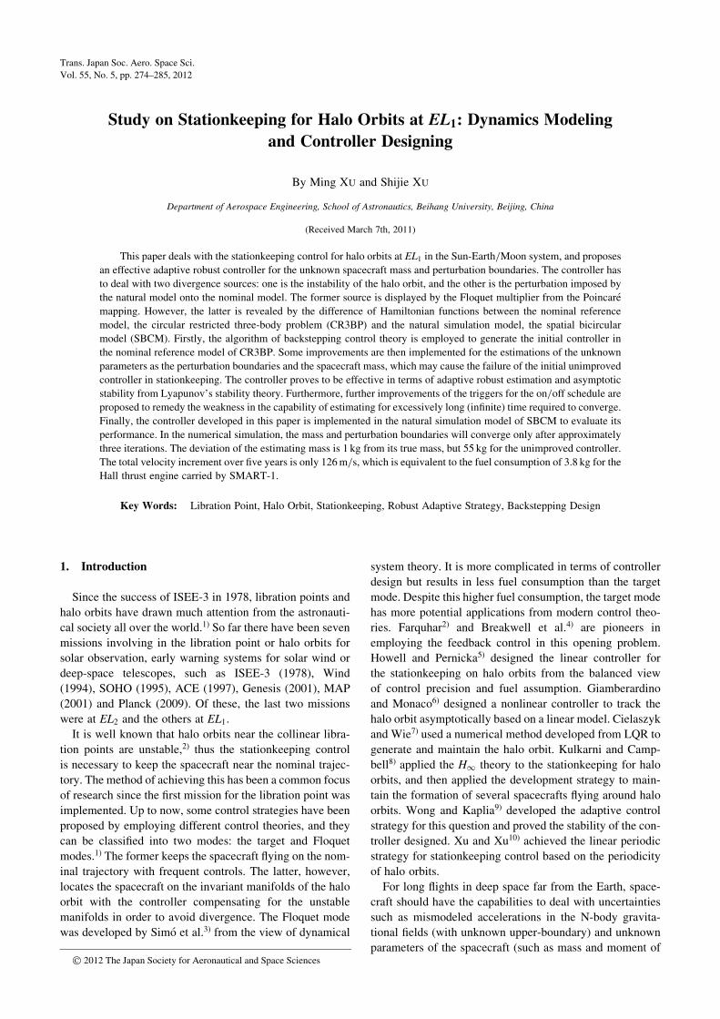
SunEarth
MoonAss
C
Rr
Spacecraft
Lunarplane:N
: EclipticplaneM
θ ϕ
Fig. 1. SBCM.
276 Trans. Japan Soc. Aero. Space Sci. Vol. 55, No. 5
2.3.2. Kinematics in the SBCM
RI ¼ ½X Y Z�T is defined as the position vector from
the barycenter of the Sun-Earth/Moon system to the space-
craft in the frame IS-E/M, and r ¼ ½� � ��T is defined as
the position vector from the barycenter of the Earth-Moon
system to the spacecraft in the frame SE-M. �S and ’ are
the phasic angles of the Sun and Moon (shown in Fig. 1),
and i is the inclination between the ecliptic and lunar planes.
AS is defined as the position vector from the Sun to the cent-
roid OE/M in the frame IS-EM.
According to definitions of coordinate systems and
SBCM assumptions, the required relationships are listed as:
R ¼ Rzð�SÞRI ð6Þ
AS ¼ ð1� �SÞ½cos �S sin �S 0�T ð7Þ
RI ¼ Rxð�iÞRzð�’ÞrþAS ð8Þ
where Rzð�Þ and Rxð�Þ are, respectively, the elementary
transformation matrixes around the Z (or z) and X (or x)
axes. The position vector R is another form of RI in the
SS-E/M frame.
The position vector r in the SE-M frame can be obtained
from Eq. (8), as
r ¼ Rzð’ÞRxðiÞRzð��SÞ½R� ð1� �SÞe1�: ð9Þ
2.3.3. Dynamics in the SBCM
The Hamiltonian function for the SBCM in SS-E/M is18)
H1 ¼1
2p2x þ p2y þ p2z
� �� xpy þ ypx
�1� �S
rS�
mE
kr� rEk�
mM
kr� rMkð10Þ
where rS is the distance between the Sun and the spacecraft,
i.e., rS ¼ kR� ½��S 0 0�Tk. Then, the dynamics in
Hamiltonian form are
_RR ¼@H1
@P
_PP ¼ �@H1
@R¼ �
@
@R
�1
2p2x þ p2y þ p2z
� �� xpy þ ypx �
1� �S
rS
�þ
@r
@R�@
@r
�mE
kr� rEkþ
mM
kr� rMk
�8>><>>: ð11Þ
where
@r
@R¼ Rzð�SÞRxð�iÞRzð�’Þ;
and the vector r can be calculated from Eq. (9).
Expand the above dynamical equations as
€xx
€yy
€zz
264
375 ¼ �2
� _yy
_xx
0
264
375þ
x
y
0
264
375� ð1� �SÞ
Rþ �Se1
kRþ �Se1k3� Rzð�SÞRxð�iÞRzð�’Þ mE
r� rE
kr� rEk3þ mM
r� rM
kr� rMk3
� �: ð12Þ
2.3.4. Alternating gravitation caused by the moon
The SBCM considers the Earth and Moon as two different
gravitational points, so that the gravitational force from the
Moon will impose the periodic perturbation on the CR3BP,
which can be measured by the difference of Hamiltonian
functions as �H ¼ H1 � H0.19) When the spacecraft stays
near the halo orbit at EL1, there exists the relationship krk �4 � k �RRE-Mk (where �RRE-M is 384,400 km, the average distance
between the Earth and Moon). Then we can attain the fol-
lowing proposition:
Proposition 1. For spacecraft flying on the halo orbit
near EL1 (or EL2), the periodic alternating gravitation is on-
ly small perturbation.
Proof. The location of OE/M in the SE/M frame is
½0 0 0�T, and the fact of rE-M ¼ krk ensures the expan-
sion of �H as
�H ¼ H1 � H0 ¼�S
rE-M�
mE
kr� rEk�
mM
kr� rMk
¼�S
krk1�
mE
�S
�r
r� rE
� mM
�S
�r
r� rM
� �:
We can transfer the mathematical expression as kak=kaþ bk as follows:
kakkaþ bk
¼
ffiffiffiffiffiffiffiffiffiffiffiffiffiffiffiffiffiffiffiffiffiffiffiffiffiffiffiffiffiffiffiaTa
ðaþ bÞTðaþ bÞ
s
¼�1þ 2
aTb
aTaþ
bTb
aTa
�12
¼ 1�aTb
kak2�
1
2
kbk2
kak2þ
3
2
ðaTbÞ2
kak4þ O
�kbkkak
3
:
ð13ÞTherefore, with the help of the above transformation tech-
nique and the following identical equation:
mErE þ mMrM ¼ 0 ð14Þ
we can deduce the simplified form of �H as
Sep. 2012 M. XU and S. XU: Study on Stationkeeping for Halo Orbits at EL1 277
�H ¼�S
krk1�
mE
�S
� 1þrTrE
krk2�
1
2
krEk2
krk2þ
3
2
ðrTrEÞ2
krk4þ o
�krEkkrk
2 !" #
��S
krkmM
�S
� 1þrTrE
krk2�
1
2
krMk2
krk2þ
3
2
ðrTrMÞ2
krk4þ o
�krMkkrk
2 !" #
:
The mass ratios of the Earth and Moon in the Sun-Earth/Moon system are as follows:
�M :¼mM
�S
� 0:01215; �E :¼mE
�S
with the identical relationship of �E þ �M ¼ 1. Thus, �H can be expressed as:
�H ¼ ��S
krk�
�EkrEk2 þ �MkrMk2
2krk2þ
3
2
rTrTð�ErErE þ �MrMrMÞkrk4
þ o
�RE-M
krk
2" #
¼ ��S
krk�
R2E-M
2krk2ð�E�
2M þ �M�
2EÞ þ
3
2
R2E-Mx
2
krk4ð�E�
2M þ �M�
2EÞ þ o
�RE-M
krk
2" #
¼ ��S
krkð�E�
2M þ �M�
2EÞ
R2E-M
krk2
��
1
2þ
3
2
x2
krk2þ oð1Þ
�
where rErE and rMrM represent the dyadic matrixes gener-
ated from the position vectors rE and rM of the Earth and
Moon in SE/M, respectively.
For spacecraft flying in the vicinity of EL1, the distance
from the Earth to the spacecraft is about four times larger
than the distance between the Earth and Moon. So we can
obtain an interesting consequence as
�H � 7:5� 10�4 ��S
krk¼ 7:5� 10�4 � UE-M: ð15Þ
According to the analysis on the energy of the halo orbit per-
formed in section 3.1.3, we can attain
H0
UE-M
� 1:5: ð16Þ
That is,H0 andUE-M are in the same order of magnitude. As-
sociated with �H � 7:4� 10�4 � UE-M, �H=H0 is of 10�3
order of magnitude, which can be considered a small pertur-
bation onto the Hamiltonian system H0.
3. Nominal Trajectory for Stationkeeping
The halo orbit, which bifurcates from the planar Lyapu-
nov orbit,8) is another solution of the CR3BP (quite different
from the fixed libration points), and is symmetrical with
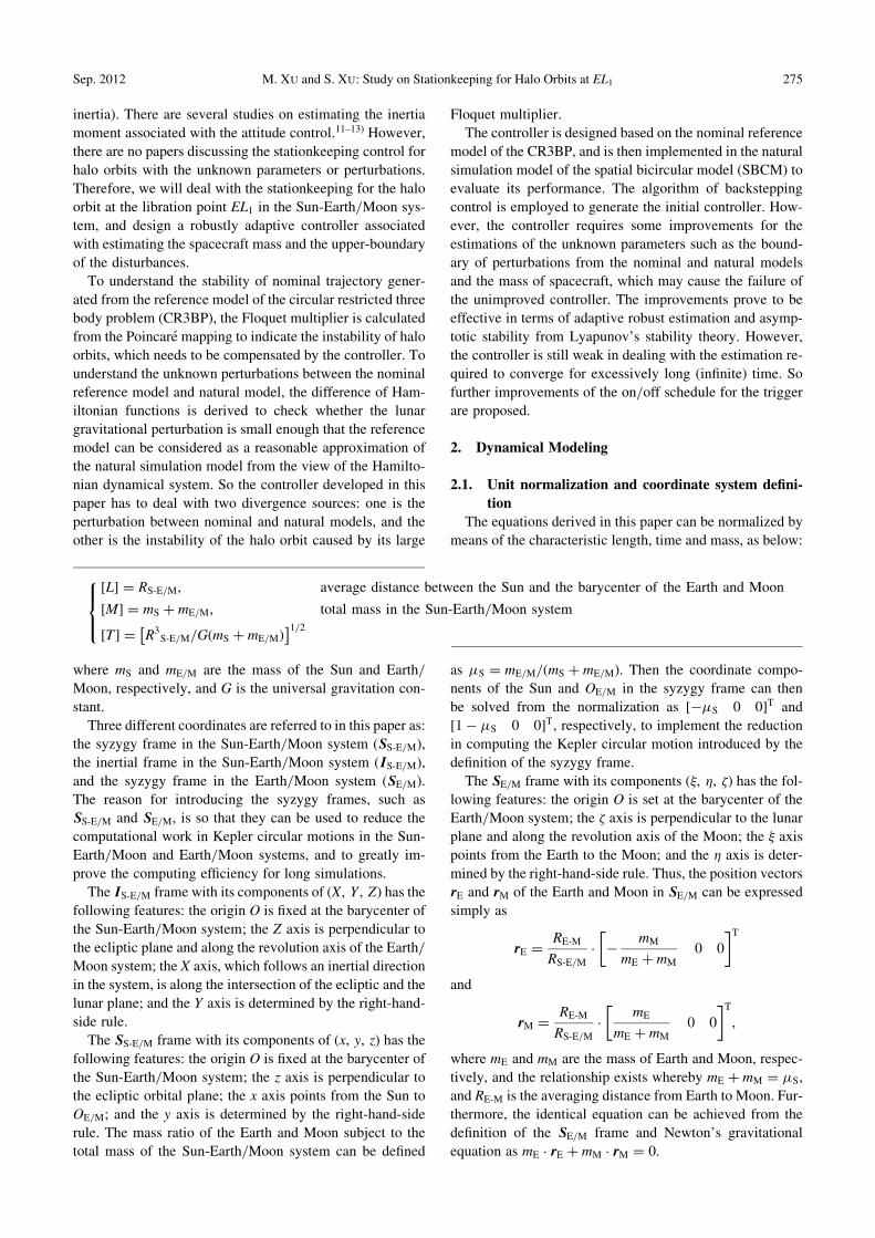
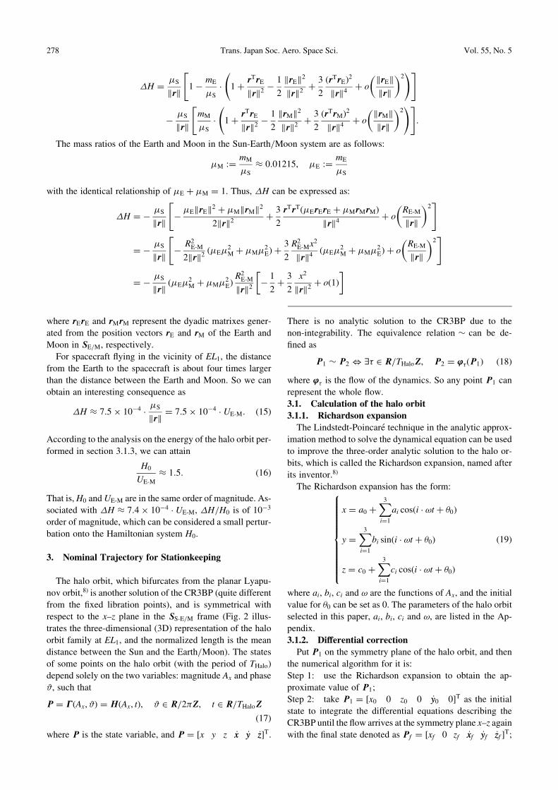
respect to the x–z plane in the SS-E/M frame (Fig. 2 illus-
trates the three-dimensional (3D) representation of the halo
orbit family at EL1, and the normalized length is the mean
distance between the Sun and the Earth/Moon). The states
of some points on the halo orbit (with the period of THalo)
depend solely on the two variables: magnitude Ax and phase
#, such that
P ¼ � ðAx; #Þ ¼ HðAx; tÞ; # 2 R=2�Z; t 2 R=THaloZ
ð17Þ
where P is the state variable, and P ¼ ½x y z _xx _yy _zz�T.
There is no analytic solution to the CR3BP due to the
non-integrability. The equivalence relation � can be de-
fined as
P1 � P2 , 9� 2 R=THaloZ; P2 ¼ ’�ðP1Þ ð18Þ
where ’� is the flow of the dynamics. So any point P1 can
represent the whole flow.
3.1. Calculation of the halo orbit
3.1.1. Richardson expansion
The Lindstedt-Poincare technique in the analytic approx-
imation method to solve the dynamical equation can be used
to improve the three-order analytic solution to the halo or-
bits, which is called the Richardson expansion, named after
its inventor.8)
The Richardson expansion has the form:
x ¼ a0 þX3i¼1
ai cosði � !t þ �0Þ
y ¼X3i¼1
bi sinði � !t þ �0Þ
z ¼ c0 þX3i¼1
ci cosði � !t þ �0Þ
8>>>>>>>>>><>>>>>>>>>>:
ð19Þ
where ai, bi, ci and ! are the functions of Ax, and the initial
value for �0 can be set as 0. The parameters of the halo orbit
selected in this paper, ai, bi, ci and !, are listed in the Ap-
pendix.
3.1.2. Differential correction
Put P1 on the symmetry plane of the halo orbit, and then
the numerical algorithm for it is:
Step 1: use the Richardson expansion to obtain the ap-
proximate value of P1;
Step 2: take P1 ¼ ½x0 0 z0 0 _yy0 0�T as the initial
state to integrate the differential equations describing the
CR3BP until the flow arrives at the symmetry plane x–z again
with the final state denoted as P f ¼ ½xf 0 zf _xxf _yyf _zzf �T;
278 Trans. Japan Soc. Aero. Space Sci. Vol. 55, No. 5
Step 3: iterate x0 and _yy0 to adjust _xxf and _zzf closed to zero
after four to five iterations.
The correction of x0 and _yy0 are:
x0
_yy0
� �¼
�41 ��21
€xxf
_yyf�45 ��25
€xxf
_yyf
�61 ��21
€zzf
_yyf�65 ��25
€zzf
_yyf
26664
37775
�1
�_xxf
_zzf
� �ð20Þ
where � is the monodromy symplectic matrix defined in
section 3.2, and �ij is the element of the matrix in the ith
row and jth column.
3.1.3. Energy allocation of the halo orbit
The Hamiltonian function H0 of the halo orbit is constant
due to the time-independent system of the CR3BP. Define
US :¼ �ð1� �SÞ=rS as the potential energy for the Sun’s
gravity, and define UE-M :¼ �ð1� �SÞ=krk as the potential
energy for the Earth’s and lunar gravities. Furthermore, de-
fine VK :¼ ð _xx2 þ _yy2 þ _zz2Þ=2 as the relative kinetic energy,
and define UC :¼ �ðx2 þ y2Þ=2 as the Coriolis potential en-
ergy. Then the Hamiltonian function is the sum of all the
variables defined above:
H0 ¼ US þ UE-M þ UC þ VK: ð21Þ
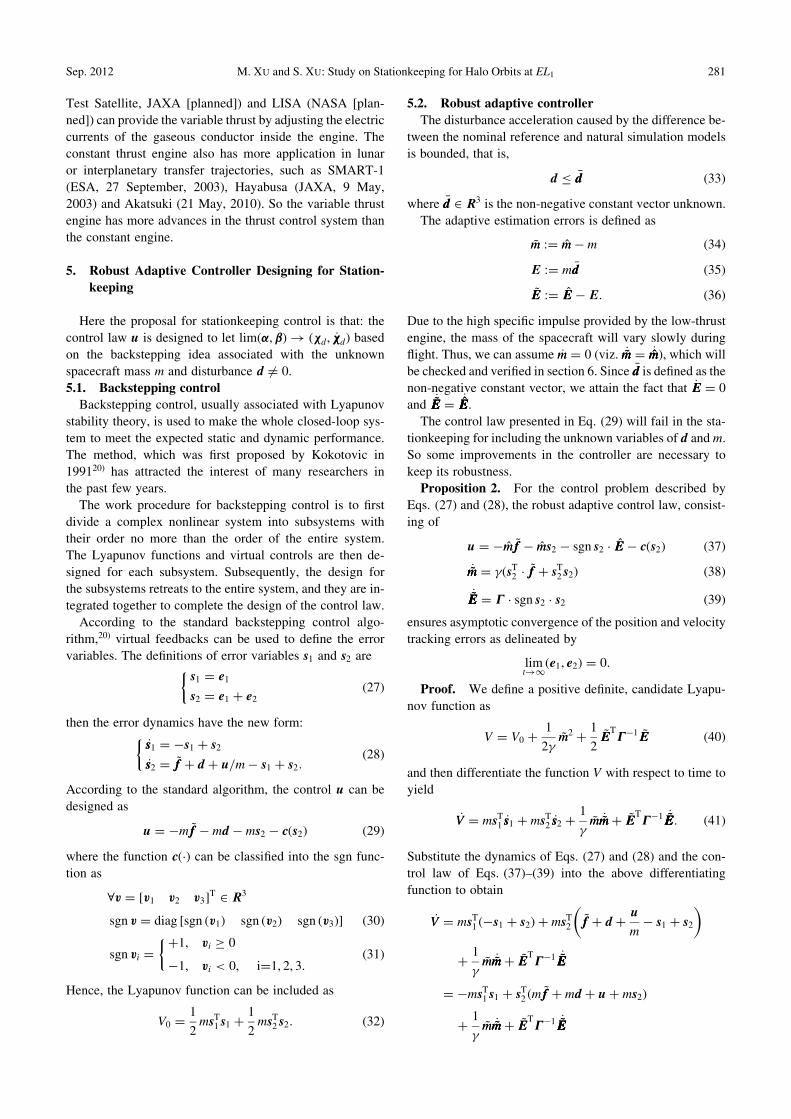
The energy allocation of the four different variables for the
halo orbit with H0 ¼ �1:5004 (with the magnitude of
Ax ¼ 260;000 km) is shown in Fig. 3.
However,US,UE-M, VK andUC all change over time, with
the exception of H0 only, and the time averages of them are
�3� 10�4, �1:0092, 4� 10�5 and �0:4909, respectively,
where the time average is calculated as
h f i ¼1
THalo
Z THalo
0
f ðtÞdt; f ¼ US;UE-M;VK;UC: ð22Þ
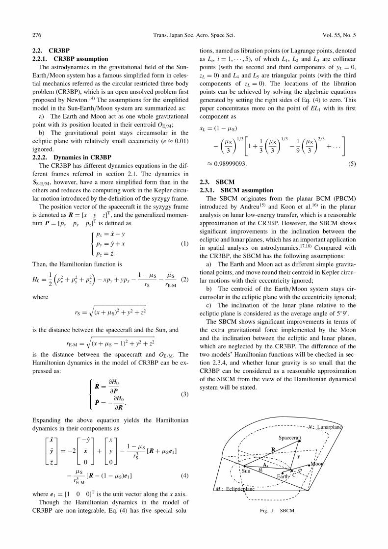
3.2. Stability analysis on halo orbits
Poincare mapping ðPÞ is defined as
ðPÞ ¼ ’THaloðPÞ; 8P 2 � ðAx; #Þ:
Then according to the Hamiltonian dynamical system, the
derivative function of ðPÞ: � ¼ DPðPÞ is a symplectic
matrix with four plural eigenvalues j�ji ¼ 1, i ¼ 1; 2; 3; 4
and two real eigenvalues �5 ¼ ��16 > 1 (the eigenvalues
of � are called characteristic exponents of the flow). �5and �6 indicate the stability of halo orbits.
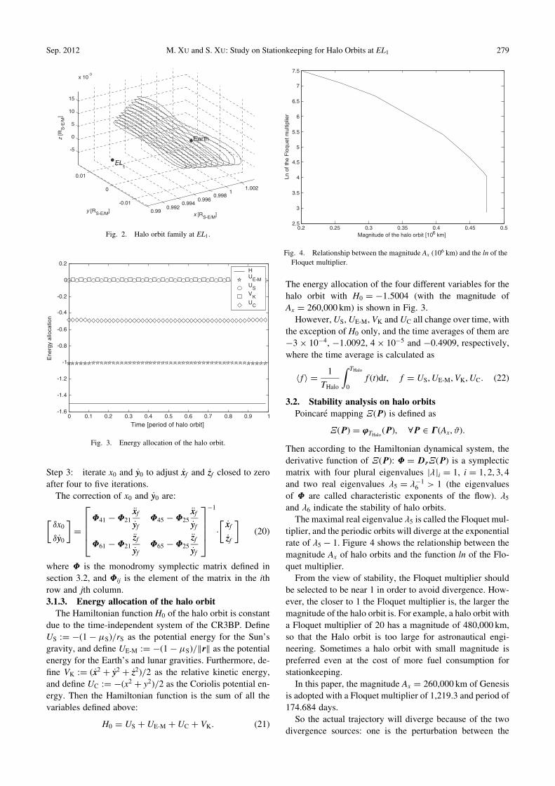
The maximal real eigenvalue �5 is called the Floquet mul-
tiplier, and the periodic orbits will diverge at the exponential
rate of �5 � 1. Figure 4 shows the relationship between the
magnitude Ax of halo orbits and the function ln of the Flo-
quet multiplier.
From the view of stability, the Floquet multiplier should
be selected to be near 1 in order to avoid divergence. How-
ever, the closer to 1 the Floquet multiplier is, the larger the
magnitude of the halo orbit is. For example, a halo orbit with
a Floquet multiplier of 20 has a magnitude of 480,000 km,
so that the Halo orbit is too large for astronautical engi-
neering. Sometimes a halo orbit with small magnitude is
preferred even at the cost of more fuel consumption for
stationkeeping.
In this paper, the magnitude Ax ¼ 260;000 km of Genesis
is adopted with a Floquet multiplier of 1,219.3 and period of
174.684 days.
So the actual trajectory will diverge because of the two
divergence sources: one is the perturbation between the
0 0.1 0.2 0.3 0.4 0.5 0.6 0.7 0.8 0.9 1-1.6
-1.4
-1.2
-1
-0.8
-0.6
-0.4
-0.2
0
0.2HU
E-MUSV
KU
C
Ene
rgy
allo
catio
n
Time [period of halo orbit]
Fig. 3. Energy allocation of the halo orbit.
0.2 0.25 0.3 0.35 0.4 0.45 0.52.5
3
3.5
4
4.5
5
5.5
6
6.5
7
7.5
Ln o
f the
Flo
quet
mul
tiplie
r
Magnitude of the halo orbit [106 km]
Fig. 4. Relationship between the magnitude Ax (106 km) and the ln of the
Floquet multiplier.
0.990.992
0.9940.996
0.9981
1.002
-0.01
0
0.01
-5
0
5
10
15
x 10-3
x [RS-E/M]y [RS-E/M]
z [R
S-E
/M]
EL1
Earth
Fig. 2. Halo orbit family at EL1.
Sep. 2012 M. XU and S. XU: Study on Stationkeeping for Halo Orbits at EL1 279
nominal and natural models, and the other is the instability
of the halo orbit caused by its large Floquet multiplier. For
the initial insertion errors in position and velocity listed in
section 6, it is no more than half an orbital period (approx-
imately three months) that the spacecraft can keep flying
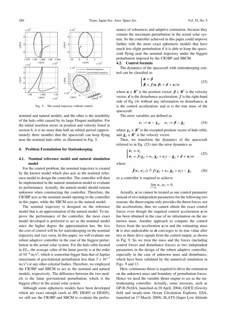
near the nominal halo orbit, as illustrated in Fig. 5.
4. Problem Formulation for Stationkeeping
4.1. Nominal reference model and natural simulation
model
For the control problem, the nominal trajectory is created
by the known model which also acts as the nominal refer-
ence model to design the controller. The controller will then
be implemented in the natural simulation model to evaluate
its performance. Actually, the natural model should remain
unknown when constructing the controller. Therefore, the
CR3BP acts as the nominal model opening to the controller
in this paper, while the SBCM acts as the natural model.
The nominal trajectory is designed on the reference
model that is an approximation of the natural model. To im-
prove the performance of the controller, the most exact
model developed is preferred to act as the nominal model
since the higher degree the approximation has, the less
the cost of control will be for stationkeeping on the nominal
trajectory and vice versa. In this paper, we will evaluate our
robust adaptive controller in the case of the biggest pertur-
bation in the actual solar system. For the halo orbit located
in EL1, the average value of the lunar gravity is at the order
of 10�6 m/s2, which is somewhat bigger than that of Jupiter
(maximum of gravitational perturbation less than 3� 10�7
m/s2) or any other celestial bodies. Therefore, we employed
the CR3BP and SBCM to act as the nominal and natural
models, respectively. The difference between the two mod-
els is the lunar gravitational perturbation, which is the
biggest effect in the actual solar system.
Although some ephemeris models have been developed
which are exact enough (such as JPL DE403 or DE405),
we still use the CR3BP and SBCM to evaluate the perfor-
mance of robustness and adaptive estimation, because they
contain the maximum perturbation in the actual solar sys-
tem. So the controller achieved in this paper could improve
further with the more exact ephemeris models that have
much less slight perturbation if it is able to keep the space-
craft flying near the nominal trajectory under the biggest
perturbation imposed by the CR3BP and SBCM.
4.2. Control formula
The dynamics of the spacecraft with stationkeeping con-
trol can be classified as
_�� ¼ �
_�� ¼ f ð�;�Þ þ d þ u=m
�ð23Þ
where � 2 R3 is the position vector; � 2 R3 is the velocity
vector; d is the disturbance acceleration; f is the right-hand
side of Eq. (4) without any information on disturbance; u
is the control acceleration; and m is the true mass of the
spacecraft.
The error variables are defined as
e1 :¼ �� �d; e2 :¼ �� _��d ð24Þ
where �d 2 R3 is the excepted position vector of halo orbit,
and _��d 2 R3 is the velocity vector.
Then, we transform the dynamics of the spacecraft
referred to in Eq. (23) into the error dynamics as
_ee1 ¼ e2
_ee2 ¼ f ð�d þ e1; _��d þ e2Þ � €��d þ d þ u=m
�ð25Þ
where
~ff ðe1; e2; tÞ , f ð�d þ e1; _��d þ e2Þ � €��d ð26Þ
so a controller is required to achieve
limt!1
e1; e2 ¼ 0:
Actually, u=m cannot be treated as one control parameter
instead of two independent parameters for the following two
reasons: the thrust engine only provides the thrust forces, not
the accelerations, thus we cannot obtain the exact control
forces even though the required control acceleration u=m
has been obtained in the case of no information on the un-
known mass. Another approach to compute the control
forces from the acceleration u=m and the estimating mass
mm is also undesirable as mm converges to its true value after
two or three drive signals from the control output, as shown
in Fig. 9. So we treat the mass and the forces (including
control forces and disturbance forces) as two independent
parameters in the design of the robust adaptive controller,
especially in the case of unknown mass and disturbance,
which have been validated by the numerical simulation in
Figs. 9 and 11.
Here, continuous thrust is required to drive the estimation
on the unknown mass and boundary of perturbation forces.
Hence we need the variable thrust engine to act as the sta-
tionkeeping controller. Actually, some missions, such as
GP-B (NASA, launched on 20 April, 2004), GOCE (Gravity
field and steady-state Ocean Circulation Explorer, ESA,
launched on 17 March, 2009), SLATS (Super Low Altitude
1.475 1.48 1.485 1.49 1.495
x 108
-5
0
5
x 105
x [km]
y [k
m]
-10 -5 0 5
x 105
-5
0
5
x 105
z [km]y
[km
]
1.48 1.485 1.49
x 108
-4
-2
0
2
4x 10
5
x [km]
z [k
m]
1.481.4821.4841.4861.488x 10
8-50
5
x 105
-4-2024
x 105
z [km]y [km]
z [k
m]
Nominal trajectory
Uncontrolled trajectory
Fig. 5. The actual trajectory without control.
280 Trans. Japan Soc. Aero. Space Sci. Vol. 55, No. 5
Test Satellite, JAXA [planned]) and LISA (NASA [plan-
ned]) can provide the variable thrust by adjusting the electric
currents of the gaseous conductor inside the engine. The
constant thrust engine also has more application in lunar
or interplanetary transfer trajectories, such as SMART-1
(ESA, 27 September, 2003), Hayabusa (JAXA, 9 May,
2003) and Akatsuki (21 May, 2010). So the variable thrust
engine has more advances in the thrust control system than
the constant engine.
5. Robust Adaptive Controller Designing for Station-
keeping
Here the proposal for stationkeeping control is that: the
control law u is designed to let limð�;�Þ ! ð�d; _��dÞ basedon the backstepping idea associated with the unknown
spacecraft mass m and disturbance d 6¼ 0.
5.1. Backstepping control
Backstepping control, usually associated with Lyapunov
stability theory, is used to make the whole closed-loop sys-
tem to meet the expected static and dynamic performance.
The method, which was first proposed by Kokotovic in
199120) has attracted the interest of many researchers in
the past few years.
The work procedure for backstepping control is to first
divide a complex nonlinear system into subsystems with
their order no more than the order of the entire system.
The Lyapunov functions and virtual controls are then de-
signed for each subsystem. Subsequently, the design for
the subsystems retreats to the entire system, and they are in-
tegrated together to complete the design of the control law.
According to the standard backstepping control algo-
rithm,20) virtual feedbacks can be used to define the error
variables. The definitions of error variables s1 and s2 are
s1 ¼ e1
s2 ¼ e1 þ e2
�ð27Þ
then the error dynamics have the new form:
_ss1 ¼ �s1 þ s2
_ss2 ¼ ~ff þ d þ u=m� s1 þ s2:
�ð28Þ
According to the standard algorithm, the control u can be
designed as
u ¼ �m ~ff � md � ms2 � cðs2Þ ð29Þ
where the function cð�Þ can be classified into the sgn func-
tion as
8v ¼ ½v1 v2 v3�T 2 R3
sgn v ¼ diag ½sgn ðv1Þ sgn ðv2Þ sgn ðv3Þ� ð30Þ
sgn vi ¼þ1; vi � 0
�1; vi < 0, i=1, 2, 3.
�ð31Þ
Hence, the Lyapunov function can be included as
V0 ¼1
2msT1 s1 þ
1
2msT2 s2: ð32Þ
5.2. Robust adaptive controller
The disturbance acceleration caused by the difference be-
tween the nominal reference and natural simulation models
is bounded, that is,
d �dd ð33Þ
where �dd 2 R3 is the non-negative constant vector unknown.
The adaptive estimation errors is defined as
~mm :¼ mm� m ð34Þ
E :¼ m �dd ð35Þ
~EE :¼ EE�E: ð36Þ
Due to the high specific impulse provided by the low-thrust
engine, the mass of the spacecraft will vary slowly during
flight. Thus, we can assume _mm ¼ 0 (viz. _~mm~mm ¼ _mmmm), which will
be checked and verified in section 6. Since �dd is defined as the
non-negative constant vector, we attain the fact that _EE ¼ 0
and _~EE~EE ¼ _EEEE.
The control law presented in Eq. (29) will fail in the sta-
tionkeeping for including the unknown variables of d andm.
So some improvements in the controller are necessary to
keep its robustness.
Proposition 2. For the control problem described by
Eqs. (27) and (28), the robust adaptive control law, consist-
ing of
u ¼ �mm ~ff � mms2 � sgn s2 � EE� cðs2Þ ð37Þ
_~mm~mm ¼ �ðsT2 � ~ff þ sT2 s2Þ ð38Þ
_~EE~EE ¼ � � sgn s2 � s2 ð39Þ
ensures asymptotic convergence of the position and velocity
tracking errors as delineated by
limt!1
ðe1; e2Þ ¼ 0:
Proof. We define a positive definite, candidate Lyapu-
nov function as
V ¼ V0 þ1
2�~mm2 þ
1
2~EET��1 ~EE ð40Þ
and then differentiate the function V with respect to time to
yield
_VV ¼ msT1 _ss1 þ msT2 _ss2 þ1
�~mm _~mm~mmþ ~EE
T��1 _~EE~EE: ð41Þ
Substitute the dynamics of Eqs. (27) and (28) and the con-
trol law of Eqs. (37)–(39) into the above differentiating
function to obtain
_VV ¼ msT1 ð�s1 þ s2Þ þ msT2
�~ff þ d þ
u
m� s1 þ s2
þ1
�~mm _~mm~mmþ ~EE
T��1 _~EE~EE
¼ �msT1 s1 þ sT2 ðm ~ff þ md þ uþ ms2Þ
þ1
�~mm _~mm~mmþ ~EE
T��1 _~EE~EE
Sep. 2012 M. XU and S. XU: Study on Stationkeeping for Halo Orbits at EL1 281
and then substitute the control law of Eq. (37) to yield
_VV ¼ �msT1 s1 þ sT2 ð� ~mm ~ff � ~mms2 þ md � sgn s2EEÞ � sT2#ðs2Þ
þ1
�~mm _~mm~mmþ ~EE
T��1 _~EE~EE
¼ �msT1 s1 � sT2#ðs2Þ þ sT2 ðmd � sgn s2 �EÞ
þ ~mm
�� sT2
~ff � sT2 s2 þ1
�_~mm~mm
þ ~EE
Tð��1 _~EE~EE� sgn s2 � s2Þ:
Furthermore, we substitute the parameter update law of
Eqs. (38) and (39) to obtain
_VV ¼ �msT1 s1 � zT2#ðs2Þ þ sT2 ðmd � sgn s2 �EÞ
sT2 ðmd � sgn s2 �EÞ:Obviously, the inequality sT2 ðmd � sgn s2 �EÞ 0 is estab-
lished constantly. The necessary and sufficient condition
for _VV ¼ 0 is s1 ¼ 0, s2 ¼ 0. According to the Lyapunov the-
orem, we can conclude that
limt!1
ðe1; e2Þ ¼ 0:
5.3. Improvements in adaptive estimation
The stationkeeping strategy proposed in the above section
is weak in terms of adaptive estimation (the numerical sim-
ulation for the primary controller is implemented in section
6, and the estimation for the unknown mass is shown in
Fig. 10).
In fact, the weakness in estimating parameters is inherited
from the initial theory of adaptive control. To estimate the
unknown parameters on a line requires the drive signals
from the control output. However, the control output will
decline quickly upon the decreasing errors in position and
velocity, and it will weaken the capability of estimation
on the line especially after the errors of states have been
converged to zero.
In order to maintain the vitality of the capability of esti-
mation, continuous drive signals from the control output
are required. So we attempt to introduce the on/off schedule
for the thrust. The thrust will be controlled by the robust
adaptive law during the on time intervals, and has no output
during the off time intervals. The trigger for the controller is
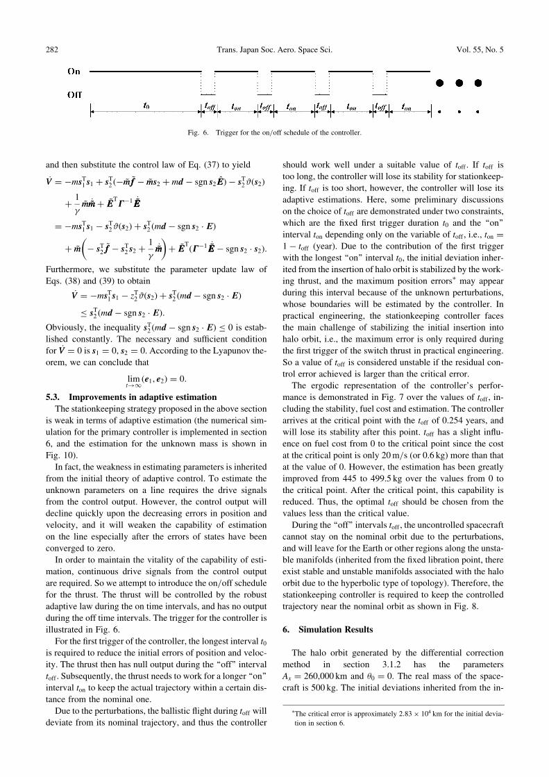
illustrated in Fig. 6.
For the first trigger of the controller, the longest interval t0is required to reduce the initial errors of position and veloc-
ity. The thrust then has null output during the ‘‘off’’ interval
toff . Subsequently, the thrust needs to work for a longer ‘‘on’’
interval ton to keep the actual trajectory within a certain dis-
tance from the nominal one.
Due to the perturbations, the ballistic flight during toff will
deviate from its nominal trajectory, and thus the controller
should work well under a suitable value of toff . If toff is
too long, the controller will lose its stability for stationkeep-
ing. If toff is too short, however, the controller will lose its
adaptive estimations. Here, some preliminary discussions
on the choice of toff are demonstrated under two constraints,
which are the fixed first trigger duration t0 and the ‘‘on’’
interval ton depending only on the variable of toff , i.e., ton ¼1� toff (year). Due to the contribution of the first trigger
with the longest ‘‘on’’ interval t0, the initial deviation inher-
ited from the insertion of halo orbit is stabilized by the work-
ing thrust, and the maximum position errors may appear
during this interval because of the unknown perturbations,
whose boundaries will be estimated by the controller. In
practical engineering, the stationkeeping controller faces
the main challenge of stabilizing the initial insertion into
halo orbit, i.e., the maximum error is only required during
the first trigger of the switch thrust in practical engineering.
So a value of toff is considered unstable if the residual con-
trol error achieved is larger than the critical error.
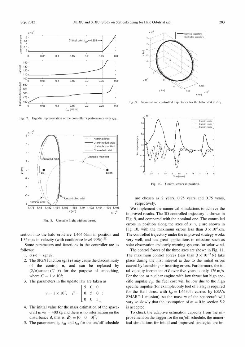
The ergodic representation of the controller’s perfor-
mance is demonstrated in Fig. 7 over the values of toff , in-
cluding the stability, fuel cost and estimation. The controller
arrives at the critical point with the toff of 0.254 years, and
will lose its stability after this point. toff has a slight influ-
ence on fuel cost from 0 to the critical point since the cost
at the critical point is only 20m/s (or 0.6 kg) more than that
at the value of 0. However, the estimation has been greatly
improved from 445 to 499.5 kg over the values from 0 to
the critical point. After the critical point, this capability is
reduced. Thus, the optimal toff should be chosen from the
values less than the critical value.
During the ‘‘off’’ intervals toff , the uncontrolled spacecraft
cannot stay on the nominal orbit due to the perturbations,
and will leave for the Earth or other regions along the unsta-
ble manifolds (inherited from the fixed libration point, there
exist stable and unstable manifolds associated with the halo
orbit due to the hyperbolic type of topology). Therefore, the
stationkeeping controller is required to keep the controlled
trajectory near the nominal orbit as shown in Fig. 8.
6. Simulation Results
The halo orbit generated by the differential correction
method in section 3.1.2 has the parameters
Ax ¼ 260;000 km and �0 ¼ 0. The real mass of the space-
craft is 500 kg. The initial deviations inherited from the in-
Fig. 6. Trigger for the on/off schedule of the controller.
The critical error is approximately 2:83� 104 km for the initial devia-
tion in section 6.
282 Trans. Japan Soc. Aero. Space Sci. Vol. 55, No. 5
sertion into the halo orbit are 1,464.6 km in position and
1.35m/s in velocity (with confidence level 99%).21)
Some parameters and functions in the controller are as
follows:
1. cðs2Þ ¼ sgn s2;
2. The SIGN function sgn ðvÞmay cause the discontinuity
of the control u, and can be replaced by
ð2=�Þ arctan ðG � vÞ for the purpose of smoothing,
where G ¼ 1� 104;
3. The parameters in the update law are taken as
� ¼ 1� 107; ¼5 0 0
0 5 0
0 0 5
264
375;
4. The initial value for the mass estimation of the space-
craft is mm0 ¼ 400 kg and there is no information on the
disturbance d, that is, EE0 ¼ ½0 0 0�T;5. The parameters t0, toff and ton for the on/off schedule
are chosen as 2 years, 0.25 years and 0.75 years,
respectively.
We implement the numerical simulations to achieve the
improved results. The 3D-controlled trajectory is shown in
Fig. 9, and compared with the nominal one. The controlled
errors in position along the axes of x, y, z are shown in
Fig. 10, with the maximum errors less than 3� 104 km.
The controlled trajectory under the improved strategy works
very well, and has great applications to missions such as
solar observation and early warning systems for solar wind.
The control forces of the three axes are shown in Fig. 11.
The maximum control forces (less than 3� 10�3 N) take
place during the first interval t0 due to the initial errors
caused by launching or inserting errors. Furthermore, the to-
tal velocity increment �V over five years is only 126m/s.
For the ion or nuclear engine with low thrust but high spe-
cific impulse Isp, the fuel cost will be low due to the high
specific impulse (for example, only fuel of 3.8 kg is required
for the Hall thrust with Isp ¼ 1;643:4 s carried by ESA’s
SMART-1 mission), so the mass m of the spacecraft will
vary so slowly that the assumption of _mm ¼ 0 in section 5.2
is accepted.
To check the adaptive estimation capacity from the im-
provement on the trigger for the on/off schedule, the numer-
ical simulations for initial and improved strategies are im-
1.478 1.48 1.482 1.484 1.486 1.488 1.49 1.492 1.494 1.496 1.498
x 108
-8
-6
-4
-2
0
2
4
6
8x 10
5
x [km]
y [k
m]
EL1 htraE
Unstable manifold
Nominal orbit
Controlled orbit
Uncontrolled orbit
Nominal orbit
Uncontrolled orbitUnstable manifold
Controlled orbit
Fig. 8. Unstable flight without thrust.
0 0.5 1 1.5 2 2.5 3 3.5 4 4.5 5-2
-1.5
-1
-0.5
0
0.5
1
1.5
2
2.5
3x 10
4
Time [years]
Err
or in
pos
ition
[km
]
Error in x axis
Error in y axis
Error in z axis
Fig. 10. Control errors in position.
0 0.05 0.1 0.15 0.2 0.25 0.3
33.5
44.5
5
x 104
Max
imum
err
or [k
m]
0 0.05 0.1 0.15 0.2 0.25 0.3100
110
120
130
140
∆V [m
/s]
0 0.05 0.1 0.15 0.2 0.25 0.3
450
475
500
525
550
toff [years]
Est
imat
ion
for
mas
s [k
g]
Critical point toff = 0.254
Fig. 7. Ergodic representation of the controller’s performance over toff .
1.48
1.485
x 108
-5
0
5
x 105
-4
-2
0
2
4
x 105
x [km]
y [km]
z [k
m]
Nominal trajectory
Controlled trajectory
Fig. 9. Nominal and controlled trajectories for the halo orbit at EL1.
Sep. 2012 M. XU and S. XU: Study on Stationkeeping for Halo Orbits at EL1 283
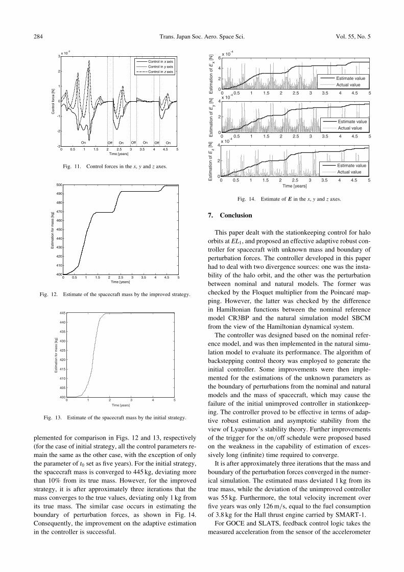
plemented for comparison in Figs. 12 and 13, respectively
(for the case of initial strategy, all the control parameters re-
main the same as the other case, with the exception of only
the parameter of t0 set as five years). For the initial strategy,
the spacecraft mass is converged to 445 kg, deviating more
than 10% from its true mass. However, for the improved
strategy, it is after approximately three iterations that the
mass converges to the true values, deviating only 1 kg from
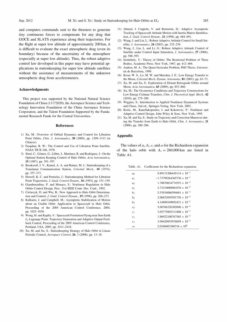
its true mass. The similar case occurs in estimating the
boundary of perturbation forces, as shown in Fig. 14.
Consequently, the improvement on the adaptive estimation
in the controller is successful.
7. Conclusion
This paper dealt with the stationkeeping control for halo
orbits at EL1, and proposed an effective adaptive robust con-
troller for spacecraft with unknown mass and boundary of
perturbation forces. The controller developed in this paper
had to deal with two divergence sources: one was the insta-
bility of the halo orbit, and the other was the perturbation
between nominal and natural models. The former was
checked by the Floquet multiplier from the Poincare map-
ping. However, the latter was checked by the difference
in Hamiltonian functions between the nominal reference
model CR3BP and the natural simulation model SBCM
from the view of the Hamiltonian dynamical system.
The controller was designed based on the nominal refer-
ence model, and was then implemented in the natural simu-
lation model to evaluate its performance. The algorithm of
backstepping control theory was employed to generate the
initial controller. Some improvements were then imple-
mented for the estimations of the unknown parameters as
the boundary of perturbations from the nominal and natural
models and the mass of spacecraft, which may cause the
failure of the initial unimproved controller in stationkeep-
ing. The controller proved to be effective in terms of adap-
tive robust estimation and asymptotic stability from the
view of Lyapunov’s stability theory. Further improvements
of the trigger for the on/off schedule were proposed based
on the weakness in the capability of estimation of exces-
sively long (infinite) time required to converge.
It is after approximately three iterations that the mass and
boundary of the perturbation forces converged in the numer-
ical simulation. The estimated mass deviated 1 kg from its
true mass, while the deviation of the unimproved controller
was 55 kg. Furthermore, the total velocity increment over
five years was only 126m/s, equal to the fuel consumption
of 3.8 kg for the Hall thrust engine carried by SMART-1.
For GOCE and SLATS, feedback control logic takes the
measured acceleration from the sensor of the accelerometer
0 0.5 1 1.5 2 2.5 3 3.5 4 4.5 50
2
4
6x 10
-4
Est
imat
ion
of E
x [N]
0 0.5 1 1.5 2 2.5 3 3.5 4 4.5 50
2
4x 10
-4
Est
imat
ion
of E
y [N]
0 0.5 1 1.5 2 2.5 3 3.5 4 4.5 50
2
4x 10
-4
Time [years]
Est
imat
ion
of E
z [N]
Estimate value
Actual value
Estimate value
Actual value
Estimate value
Actual value
Fig. 14. Estimate of E in the x, y and z axes.
0 0.5 1 1.5 2 2.5 3 3.5 4 4.5 5-3
-2
-1
0
1
2
3x 10
-3
Time [years]
Con
trol
forc
e [N
]
On Off Off Off On On On
Control in x axis
Control in y axis
Control in z axis
Fig. 11. Control forces in the x, y and z axes.
0 0.5 1 1.5 2 2.5 3 3.5 4 4.5 5400
410
420
430
440
450
460
470
480
490
500
Est
imat
ion
for
mas
s [k
g]
Time [years]
Fig. 12. Estimate of the spacecraft mass by the improved strategy.
0 1 2 3 4 5400
405
410
415
420
425
430
435
440
445
Est
imat
ion
for
mas
s [k
g]
Time [years]
Fig. 13. Estimate of the spacecraft mass by the initial strategy.
284 Trans. Japan Soc. Aero. Space Sci. Vol. 55, No. 5
and computes commands sent to the thrusters to generate
tiny continuous forces to compensate for any drag that
GOCE and SLATS experience along their trajectories. For
the flight at super low altitude of approximately 200 km, it
is difficult to evaluate the exact atmospheric drag (even its
boundary) because of the uncertainty of the atmosphere
(especially at super low altitude). Thus, the robust adaptive
control law developed in this paper may have potential ap-
plications in stationkeeping for super low altitude satellites
without the assistance of measurements of the unknown
atmospheric drag from accelerometers.
Acknowledgments
This project was supported by the National Natural Science
Foundation of China (11172020), the Aerospace Science and Tech-
nology Innovation Foundation of the China Aerospace Science
Corporation, and the Talent Foundation Supported by the Funda-
mental Research Funds for the Central Universities.
References
1) Xu, M.: Overview of Orbital Dynamics and Control for Libration
Point Orbits, Chin. J. Astronautics, 30 (2009), pp. 1299–1313 (in
Chinese).
2) Farquhar, R. W.: The Control and Use of Libration Point Satellite,
NASA TR R-346, 1970.
3) Simo, C., Gomez, G., Llibre, J., Martinez, R. and Rodriguez, J.: On the
Optimal Station Keeping Control of Halo Orbits, Acta Astronautica,
15 (1987), pp. 391–397.
4) Breakwell, J. V., Kamel, A. A. and Ratner, M. J.: Stationkeeping of a
Translunar Communication Station, Celestial Mech., 10 (1974),
pp. 357–373.
5) Howell, K. C. and Pernicka, J.: Stationkeeping Method for Libration
Point Trajectories, J. Guid. Control Dynam., 16 (1993), pp. 151–159.
6) Giamberardino, P. and Monaco, S.: Nonlinear Regulation in Halo
Orbits Control Design, Proc. 31st IEEE Contr. Dec. Conf., 1992.
7) Cielaszyk, D. and Wie, B.: New Approach to Halo Orbit Determina-
tion and Control, J. Guid. Control Dynam., 19 (1996), pp. 266–273.
8) Kulkarni, J. and Campbell, M.: Asymptotic Stabilization of Motion
about an Unable Orbit: Application to Spacecraft in Halo Orbit,
Proceeding of the 2004 American Control Conference, 2004,
pp. 1025–1030.
9) Wong, H. and Kaplia, V.: Spacecraft Formation Flying near Sun-Earth
L2 Lagrange Point: Trajectory Generation and Adaptive Output Feed-
back Control, Proceeding of the 2005 American Control Conference,
Portland, USA, 2005, pp. 2411–2418.
10) Xu, M. and Xu, S.: Stationkeeping Strategy of Halo Orbit in Linear
Periodic Control, Aerospace Control, 26, 3 (2008), pp. 13–18.
11) Ahmed, J. Coppola, V. and Bernstein, D.: Adaptive Asymptotic
Tracking of Spacecraft Attitude Motion with Inertia Matrix Identifica-
tion, J. Guid. Control Dynam., 21 (1998), pp. 684–691.
12) Wang, J. and Liu, L.: Robust Adaptive Attitude Control for Small Sat-
ellite, J. Astronautics, 24 (2003), pp. 235–239.
13) Wang, J., Liu, L. and Li, G.: Robust Adaptive Attitude Control of
Satellite under Control Input Saturation, J. Astronautics, 27 (2006),
pp. 588–593.
14) Szebehely, V.: Theory of Orbits: The Restricted Problem of Three
Bodies, Academic Press, New York, 1967, pp. 412–466.
15) Andreu, M. A.: The Quasi-bicircular Problem, PhD Thesis, Universi-
tat de Barcelona, 1999.
16) Koon, W. S., Lo, M. W. and Marsden, J. E.: Low Energy Transfer to
the Moon, Celestial Mech. Dynam. Astronomy, 81 (2001), pp. 63–73.
17) Xu, M. and Xu, S.: Exploration of Distant Retrograde Orbits around
Moon, Acta Astronautica, 65 (2009), pp. 853–860.
18) Xu, M.: The Occurrence Conditions and Trajectory Constructions for
Low Energy Cislunar Transfers, Chin. J. Theoretical Appl. Mech., 42
(2010), pp. 275–289.
19) Wiggins, S.: Introduction to Applied Nonlinear Dynamical Systems
and Chaos, 2nd ed., Springer-Verlag, New York, 2003.
20) Krstic, M., Kanellakopoulos, I. and Kokotovic, P.: Nonlinear and
Adaptive Control Design, John Wiley & Sons, New York, 1995.
21) Xu, M. and Xu, S.: Study on Trajectory and Correction Maneuver dur-
ing the Transfer from Earth to Halo Orbit, Chin. J. Aeronautics, 21
(2008), pp. 200–206.
Appendix
The values of ai, bi, ci and ! for the Richardson expansion
of the halo orbit with Ax ¼ 260;000 km are listed in
Table A1.
Table A1. Coefficients for the Richardson expansion.
a0 9:89131506445114� 10�1
a1 �1:73799264365736� 10�3
a2 1:70870834774553� 10�4
a3 2:73210089081076� 10�5
b1 5:53934086594681� 10�3
b2 2:06832695501756� 10�4
b3 4:14890349892431� 10�5
c0 5:60766326302696� 10�4
c1 3:05775892311808� 10�3
c2 1:86922108767565� 10�4
c3 3:09420953976059� 10�5
! 2:0348403360716� 100
Sep. 2012 M. XU and S. XU: Study on Stationkeeping for Halo Orbits at EL1 285