Study on Energy Use by Air- Conditioning: Annex E ... · Study on Energy Use by Air-Conditioning: Annex E: Algorithm for use with existing DECC ... Algorithm for use with existing

Study on Energy Use by Air-

Conditioning: Annex E: Algorithm

for use with existing DECC model

BRE Client Report for the Department of Energy &

Climate Change, HPR218-1001 - June 2016

Authors: Alan Abela, Lorna Hamilton, Roger

Hitchin, Andy Lewry and Christine Pout

This report provides supporting information and explanation to the DECC Report “Study on

Energy Use by Air-Conditioning: Final Report” (BRE Client Report HPR218-1001 The views

expressed in this report are those of the authors, and not necessarily those of the

Department of Energy and Climate Change (nor do they reflect Government policy).

It is published under the conditions of the Open Government Licence; i.e., this information

(not including logos) may be used free of charge in any format or medium, subject to the

terms of this Licence.

To view this licence, visit www.nationalarchives.gov.uk/doc/open-government-licence/ or

write to the Information Policy Team, The National Archives, Kew, London TW9 4DU, or

email: [email protected].

Any enquiries regarding this publication should be sent to Penny Dunbabin (email

[email protected])

BRE has used all reasonable skill and care in respect of this report but does not warrant its

accuracy or completeness. BRE does not guarantee that this report will be free from errors and

omissions.

Study on Energy Use by Air-Conditioning: Annex E: Algorithm for use with existing DECC model

1

Annex E: Algorithm for use with existing DECC model

This Annex describes the structure and use of an algorithm

developed to estimate peak and monthly electricity demand

from air-conditioning units. The algorithm can be used to

standardise the energy consumption of air conditioning

systems and components from different source data and to

improve understanding of the geographical variation of air-

conditioning energy consumption. The purpose of the

Algorithm is to enable DECC to supplement their current

model of electricity consumption from air-conditioning.

1. Objectives

1.1. A major objective of this study is to improve DECC’s modelling of electricity demand from air-conditioning systems in terms of both data quality and methodology.

1.2. At present, the [current] DECC model only predicts annual electricity demand. One of the aims of this study is to improve the model by estimating monthly and peak demand. The work to achieve this included :

1.2.1. Examining the literature and monitored data to determine how usage patterns vary as a function of temperature.

1.2.2. Improving our understanding of the geographical variation of air-conditioning deployment and use.

1.2.3. Writing an excel algorithm to estimate peak and monthly electricity demand from air-conditioning units as a function of degree days, Government Office Region and electricity price1.

1.2.4. Providing an algorithm that can be used to supplement the current DECC model of electricity consumption from air-conditioning.

1As no evidence for electricity prices impacting on energy consumption for cooling were identified, it was

not possible to include this variable in the algorithm.


2

1.2.5. This Annex addresses item 1.2.3 above but also explains how the algorithm can be used to address item 1.2.2; and, in principle, other features of energy consumption by air conditioning.

2. Features of the current DECC model

2.1. There are currently two main DECC information sources on electricity use for air conditioning in the UK. These are annual energy consumption for air conditioning published in UK Energy Consumption StatisticsA, and DECC’s product policy model for air conditioningB,2.

2.2. The statistics published in Energy Consumption in the UK are based on secondary analysis of N-DEEM (Non-Domestic Energy and Emissions Model) data. N-DEEM was a technologically disaggregated model of energy use across the UK building stock which combined end use energy consumption for different building types with building stock data. This model was used to inform policy decisions relating energy and climate change for a number of years although funding for primary data collection for NDEEM ceased in 2005. The functionality of NDEEM is effectively being replaced by two DECC initiatives, non-domestic NEED (National Energy Efficiency Database)C, which has stock level data and the BEES (Building Energy Efficiency Study) projectD, which is carrying out building energy surveys on end uses of energy.

2.2.1. DECC’s product policy model estimates aggregated annual air conditioning energy consumption based on the amount of equipment installed, its efficiency and operation. The amount of equipment installed is estimated for each product in each year, based on sales data and assumptions about average product and system lifetime.

2.2.2. For chillers and packaged air conditioning systems, the amount of equipment is expressed in terms of its maximum cooling output in kW, for Air Handling Units (AHUs) as kW of air movement, and Fan Coil Units (FCU) as kW peak electricity input. The equipment types are further disaggregated by size (kW capacity).

2.2.3. The model estimates the electricity consumption for each type of equipment based on the calculated stock of equipment for each year in kW, its expected energy efficiency and the equivalent full load hours of operation per year (referred to as “operating hours” within the model). Results are summarised for equipment >12kW and <12kW in line with the primary categorisation used for cooling in the Energy Related Products Directive.

2.2.4. The DECC product policy model considers both packaged and central air conditioning systems.

2 This is referred to as the MTP (Market Transformation Programme) model. It has been used to develop

baseline and policy scenarios for the Government’s Market Transformation Programme.


3

Packaged systems included in the model are:

Close control units

Indoor units

Wall/window units

Moveable units

Close control units

Rooftop units

Ducted split systems

Mini split systems

For central systems, it separately considers the energy consumption of the

following components:

Air-cooled chiller

Water-cooled chillers

Absorption chillers

Air Handling units (AHUs)

Fan coil units.

The following system types do not appear to be explicitly included in the model

VRF systems

Water loop heat pump systems,

Some types of legacy system (notably dual duct and terminal reheat systems)

2.2.5. It is important to note that the product policy model only assesses energy

consumption by individual products based on typical load factors (equivalent full load hours). Therefore it cannot take account of how the products will perform within a particular type of system. Neither is it able to take account of energy use by auxiliary equipment, such as controls and distribution fans, or system losses.

2.2.6. Aside from equipment size, we believe that the current model is not disaggregated in other ways, such as by market sector or geographical location.

2.2.7. Within the model the efficiency for all equipment types is referred to as a COP (Coefficient of Performance) rather than as an EER (Energy Efficiency Ratio), which is conventionally used for cooling equipment, but, as both metrics are ratio of electricity input to energy output (for heating or cooling, respectively),) this is of no consequence. However, it is not immediately apparent whether the efficiency values used in the model are snapshot values measured under specified conditions or represent the expected average annual efficiency of the equipment.

2.2.8. Energy efficiency metrics commonly used in air conditioning systems are described in more detail in the following section.

2.3. Our understanding of the way that the current model estimates aggregate annual air conditioning energy consumption is that it:


4

Estimates the stock in any year from sales data and assumptions about average

product and system lifetime.

Estimates the consequent consumption using estimates of seasonal product

efficiency (SEER) and load factor (EFLH is described as “operating hours” in the

current model).

Separately considers two types of systems, central air conditioning systems and

packaged systems

2.3.1. In principle, it separately considers the energy consumption of the following components of central systems: air-handling units, absorption chillers, air-cooled chillers, water-cooled chillers, fan coil units. In practice, it appears to focus on packaged chillers and air handling units.

2.3.2. It does not appear to explicitly include VRF systems, water loop heat pump systems, or some types of legacy system (notably dual duct and terminal reheat systems) but we assume that these are, in principle, within its scope.

2.3.3. Packaged systems include: close [control units], mini-splits, moveable [units], rooftop [units], window [units] (and presumably multi-split systems and larger single split systems)

2.3.4. The current model does not take account of the effect of annual or regional variations in weather on energy use for cooling and is not disaggregated in other ways, such as by market sector or geographical location.

3. Algorithm Principles 3.1. The algorithm that has been developed is based on “energy signatures” and

mean daily external (outdoor) temperatures. An energy signature describes the temperature dependent element of daily energy consumption across a range of specific mean daily external temperatures. Energy signatures therefore represent the relationship between external temperature and electricity consumption.

3.2. The algorithm employs mean daily average external temperature rather than cooling degree days3 (which are commonly used to determine the temperature dependence of air conditioning systems) to determine the relationship between temperature and energy consumption.

3.2.1. Using mean daily outdoor temperatures is effectively a generalisation of the assumptions that underlie degree-day analysis. Both approaches relate energy consumption to outdoor temperature and aim to separate building (and system) characteristics (including patterns of use) from climatic and weather influences. Both approaches produce figures for mean consumption on days of particular outdoor temperature: there is additional day to day variability unrelated to outdoor temperature.

3.2.2. In the case of degree-day procedures, there is an assumption that daily energy demand is a linear function of mean outdoor temperature. While this

3 Cooling degree days are the number of degrees by which that the mean daily external

temperature exceeds a specified base temperature, which is the external temperature above which cooling, typically, will be required in buildings.


5

is a reasonable approximation for most heating systems and some air conditioning systems, it is not universal - the simple linear model cannot be safely assumed. For air conditioning, non-linearities often arise from variations in the overall efficiency of the air conditioning system under different load conditions and how the building fabric performs at different external temperatures. An advantage of the energy signature approach is that it can be used with linear and non-linear relationships.

3.2.3. Unlike cooling degree days, mean average external temperatures do not presuppose a base temperature above which cooling is required. This is important because the mean daily temperature above which cooling is needed (the base temperature) can vary considerably depending on how well insulated and air tight the building is and the level of internal and solar gains through the fabric. Using mean daily temperatures negates the need to consider the base temperature for each application (building type).

3.2.4. As weather data are for specific recording sites, the mean average daily temperatures may not necessarily be representative of a region as a whole. This is potentially important as there is typically more variation within a degree-day region (and therefore a Government Office region) than there is between weather stations in adjacent regions.

3.3. Energy signatures are defined as a table of energy consumptions for different

outdoor air temperature “bins”. Ideally they would be constructed by sorting data

into “bins” of similar outdoor temperature and selecting the mean or median value

for each temperature, since this makes no assumptions about the form of the

relationship between consumption and temperature. This format also makes it

straightforward to combine energy signatures from different buildings.

3.3.1. However, constructing energy signatures in this form requires there to be

significant number of data points at each temperature. This is unlikely to be

the case for important but infrequently encountered conditions such as heat

waves, so the energy signatures derived from monitored data are based on

regressions. Bin data sets are then derived from the equations. The

regressions are mostly in the form of a continuous series of linear segments

but a few are non-linear regressions, which provide a better fit to the data.

(Section 7 explains why the linear segmental form may often be expected).

3.3.2. Typically, there will be systematic differences of energy signature between

different days of the week – notably between working and non-working days.

It is important to have a consistent convention for handling this. It is

suggested this should be to carry out a calculation full year (or month) for

each type of day before producing a weighted average that reflects the

average numbers of each type of day.

3.3.3. As energy signatures depend on the actual (or, in the case of simulations,

assumed) patterns of use of buildings and systems, they can therefore

change during or between years.


6

3.3.4. Where energy signatures are derived from empirical data, they incorporate the effect of real life operational conditions rather the idealised conditions assumed within most models. Energy signatures can therefore be applied to any type of air conditioning system or cooling equipment, and they are potentially applicable to heating systems and to any energy-using equipment that has temperature dependent components such as cooling towers and fans in variable-volume systems. Also to any section of the market, provided an energy signature and suitable temperature data are available. This could be for a single system or for a group of systems that share common features such as location, system type, or end-use. Furthermore energy signatures can be applied to any location for which a suitable set of outdoor daily mean air temperatures is available, including data sets representing the urban heat island effect or climate change projections.

3.3.5. A key requirement of the algorithm is the ability to calculate monthly energy consumption as well as annual energy consumption. The algorithm therefore calculates the proportion of the annual energy consumption which falls into each month for a given energy signature. These monthly weightings can be applied to the annual consumptions calculated by the existing model. Alternatively the annual consumption can be calculated based on the installed cooling load, the SSEER of the system and the number of equivalent full load hours.

3.3.6. Annual or monthly consumptions for a particular system are calculated as the sum of the products of the daily consumption at each daily mean outdoor temperature and the number of days at that temperature. Differences between years or locations (including city centres) can be reflected by the appropriate choice of temperature data. Sensitivities to climate change can be addressed in a similar manner. The standardisation is with respect to outdoor temperature only: systematic seasonal differences of solar gains with latitude will not be reflected. This will be more important in strongly solar-driven spaces with large glazing areas or low internal heat gains.

3.4. The algorithm is also required to calculate peak power demand. This is

comprised of two elements, the temperature dependent portion of demand and

the non-temperature dependent portion. The standardised peak half-hourly

average power demand for a system is derived from the energy signature and the

frequency distribution of residuals between half-hourly power levels and daily

mean power. There are two stages to this process :

3.4.1. Firstly, determine the mean daily electrical power for a defined daily mean

outdoor temperature, using the energy signature of the components (or

system) in question.

3.4.2. Secondly, use the residuals of half-hourly consumption from the

temperature-corrected daily mean values to add the impact of short-term non-


7

temperature-dependent contributions (time of day effects, solar variations,

other incidental gains).

3.4.3. This produces a standardised peak half-hourly demand for a system.

However, the timing of peak demand is likely to be different, even where

similar systems are installed in buildings with similar cooling demands.

Therefore, in order to estimate the aggregated peak demand at a local,

regional or national level, it will be necessary to apply a diversity factor to the

peak demands calculated using the algorithm. For a single system in a single

building, a diversity factor of 1 would apply and the value would decrease

with the number of systems that are being aggregated.

3.4.4. Further analysis is recommended to determine appropriate diversity factors

for aggregating the peak demand from air conditioning systems. In addition to

taking account of the effect of multiple systems, Monte Carlo analyses (or

similar) would need to be undertaken to determine the effect of different

cooling demand profiles for different building types and local and regional

differences in mean daily external temperatures.

3.4.5. A provisional “percentile exceeded” value of 5% is suggested when defining

the peak demand from monitored data. This value needs to provide a balance

between the risks of missing extreme values and of giving too much weight to

data errors. In a month of week days with five day per week working and 10

hours of operation per day, there would typically be about 200 data points, so

a 5 percentile value would exclude about 10 values.

3.4.6. The algorithm can potentially be configured in different ways depending on

the type of input data that is available. Two configurations are presented here

which reflect DECC’s current modelling capabilities. One where annual kWh

is the primary data input and one based on kW installed cooling capacity,

correspond to the DECC’s energy consumption statistics and to DECC’s

current product policy model, respectively. These are shown in Figure 1 and

Figure 2, respectively


8

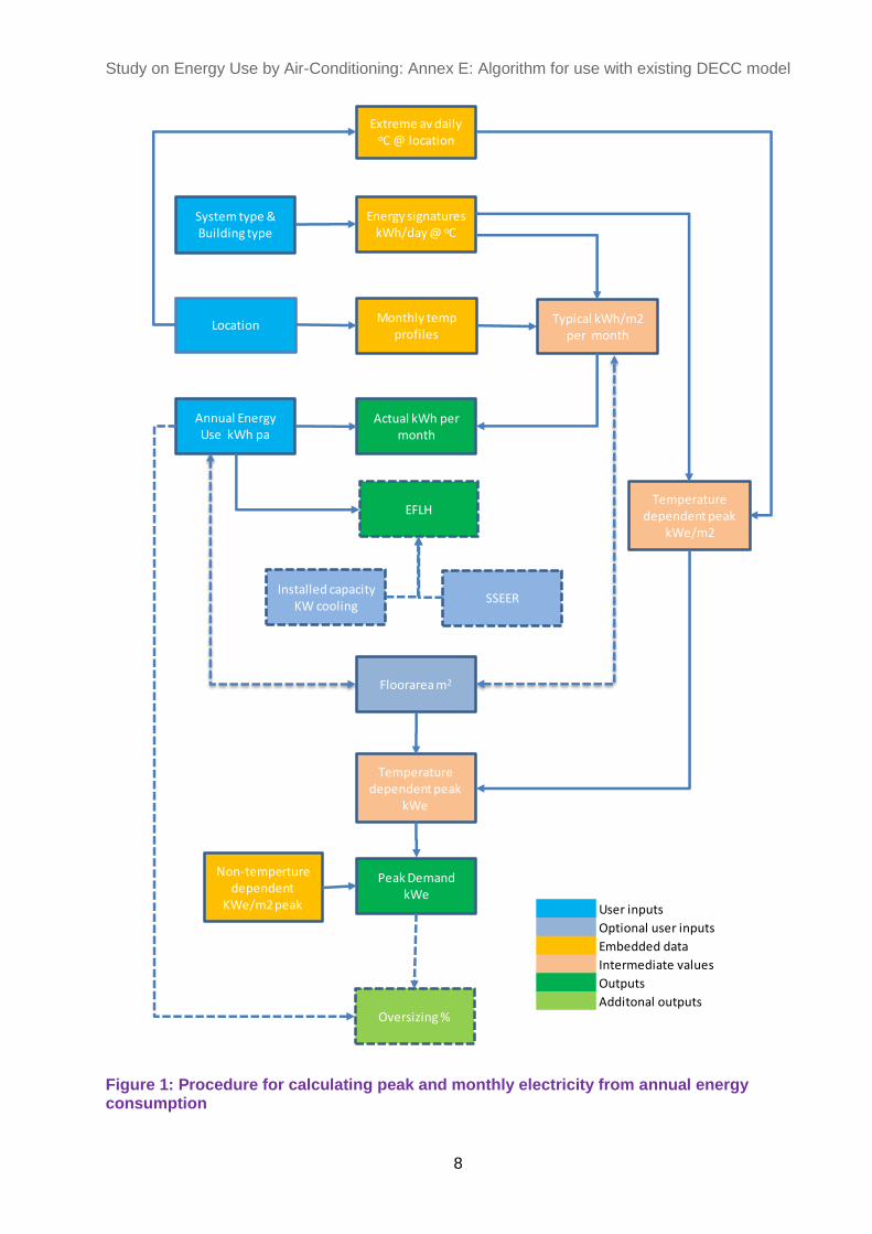
Figure 1: Procedure for calculating peak and monthly electricity from annual energy consumption

User inputs

Optional user inputs

Embedded data

Intermediate values

Outputs

Additonal outputs

Energy signatures kWh/day @ oC

Extreme av daily oC @ location

Monthly temp profiles

System type & Building type

Location

Annual Energy Use kWh pa

Floorarea m2

Non-temperture dependent

KWe/m2 peak

Installed capacityKW cooling

SSEER

Actual kWh per month

Peak Demand kWe

EFLH

Oversizing %

Typical kWh/m2 per month

Temperature dependent peak

kWe/m2


kWe


9

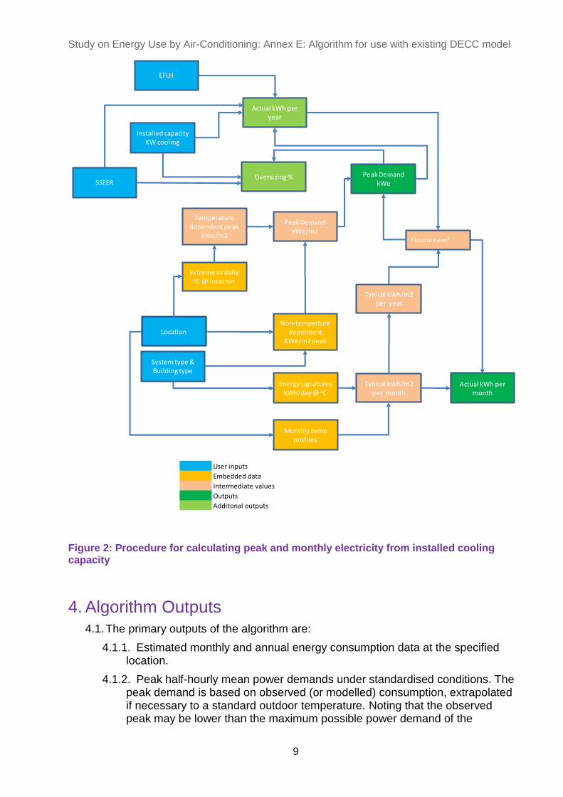
Figure 2: Procedure for calculating peak and monthly electricity from installed cooling capacity

4. Algorithm Outputs 4.1. The primary outputs of the algorithm are:

4.1.1. Estimated monthly and annual energy consumption data at the specified location.

4.1.2. Peak half-hourly mean power demands under standardised conditions. The peak demand is based on observed (or modelled) consumption, extrapolated if necessary to a standard outdoor temperature. Noting that the observed peak may be lower than the maximum possible power demand of the

User inputs

Embedded data

Intermediate values

Outputs

Additonal outputs

Energy signatures kWh/day @ oC

Extreme av daily oC @ location

Monthly temp profiles

System type & Building type

LocationNon-temperture

dependent KWe/m2 peak

Actual kWh per month

Peak Demand kWe

Oversizing %

Typical kWh/m2 per month


kWe/m2

Installed capacityKW cooling

SSEER

EFLH

Peak Demand kWe/m2

Floorarea m2

Actual kWh per year

Typical kWh/m2 per year


10

installed equipment if the system is sized generously for the actual level of heat gains.

4.1.3. Percentage oversizing can also be determined from the installed capacity and the peak demand.

4.2. These outputs can be calculated for any section of the market for which an energy signature and suitable temperature data are available. This could be for a single system or a group of systems that share common features such as location, system type, or end-use.

4.3. The impact of electricity price cannot be explicitly calculated since no information was found that would enable it to be represented.

4.4. While the emphasis of this project is on the energy used to provide cooling, the algorithm is also applicable to energy used for heating and to other energy-using components of air-conditioning systems that may have temperature-dependent consumption, such as cooling towers and fans in variable-volume systems.

5. Required Inputs

5.1. The algorithm requires the following input data in order to produce monthly weighting factors:

5.1.1. An energy signature for an air conditioning system or collection of systems

5.1.1.1. This should be in the form of a table of daily (24 hour) electricity consumption values, each associated with a 1oC range of 24-hour mean outdoor air temperatures (for example 15 oC +/- 0.5oC): these are the outdoor air temperature “bins”.

5.1.1.2. Depending on the required output, the electricity consumptions may be expressed in terms of kWh per kW of installed equipment power capacity, kWh per kW of calculated peak power demand or kWh per square metre of conditioned space.

5.1.2. The annual or monthly frequency of occurrence of each temperature bin for the location in question.

5.2. In order to produce standardised peak power demands:

5.2.1. A reference external daily mean air temperature.

5.2.2. A frequency distribution of the differences between half-hourly consumption within a day and the 24-hour daily mean electrical power for the day (daily consumption divided by 24), during periods when the air conditioning system(s) are in operation.

5.2.3. This is required to characterise the non-temperature-dependent component of demand.

5.3. The standardised load factors (equivalent full-load hours) are derived from the annual consumption and peak demand.

5.4. Since the DECC model uses cooling power (rather than electrical input power) as the functional variable, the energy signatures will require conversion into cooling energy using assumptions for efficiency figures. In principle, the variation of efficiency with outdoor temperature may be included. Allowance will also need to be made for “oversizing”, whether intentional (to provide resilience against


11

operational conditions exceeding design assumptions or against technical failure, for example) or inadvertent (such as limitations on available equipment size). The degree and frequency of over- (and under-) sizing are discussed in Annex B

6. Data Sources

6.1. Energy Signatures

6.1.1. Ideally, the energy signatures and the frequency distributions of residuals will be determined from field measurements, but they may be estimated from building and system energy simulations.

6.2. Daily temperatures

6.2.1. Whole-year daily mean air temperature data are available from several sources. The most appropriate sources in most instances are the CIBSE sets of Test Reference Years (TRY) and Summer Demand Years for 14 UK locations. Similar CIBSE datasets are available for several future climate change scenarios and adjusted for the urban heat island effect of London.

6.2.1.1. A TRY is a synthetic year constructed from elements of real years: it differs from a set of long-term average conditions by including some of the idiosyncrasies that characterise real years. Average weather, on the other hand, removes year to year variations and thereby compresses the range of daily temperatures. The algorithm may be used with either source - but the results will, of course, differ.

6.3. Half-hourly temperatures

6.3.1. A reference hourly or half-hourly outdoor temperature is required for two purposes:

To define the peak hourly power demand used to calculate standardised “equivalent full load hours” or “operating hours” for the DECC model

As an indicator of peak demand on the electricity supply system

6.3.2. For the first purpose, it seems reasonable to aim to be consistent with air conditioning system design practice. Hourly temperatures for air-conditioning design purposes are readily available, but the corresponding 24-hour mean outdoor air temperatures are not, and need to be estimated. Design peak hourly outdoor temperature varies with region and with the acceptability of indoor temperatures that exceed the target comfort conditions. For comfort cooling a criterion for outdoor temperature corresponding to the threshold for the 5 hottest hours per year on average is commonly assumed. At Heathrow this is 28.3oC. At Edinburgh it is 22.2oC. The algorithm requires a daily mean temperature that is consistent with this hourly value. From the data for the CIBSE Summer Design Year (SDY) for London, we find that the average difference between the hourly temperatures which exceed the 28.3 oC “design temperature” and the corresponding 24-hour mean temperatures of the days that contain these hours is 6.7oC. A mean outdoor air temperature of 21.6 oC therefore seems appropriate for Heathrow for general air conditioning purposes. The SDY is a synthetic weather year produced by combining periods of historical data in order to allow the simulation of building and system designs exposed to unusual but plausible weather conditions. By definition it is an unusual year, and includes 11 hours for which the outdoor temperature exceeds 28.3oC.


12

6.3.2.1. Some end-uses require a lower risk of higher external temperatures, corresponding to a more powerful cooling system and a lower risk of overheating within the space. For such applications, it would be usual to use a design temperature for Heathrow of 34.6oC. According to ASHRAE figures, this would represent a return period of nearly 20 years. The maximum hourly temperature in the Summer Design Year is only 33.6 oC, but by extrapolation we can estimate the equivalent daily mean temperature to be 28.2oC. (The highest recorded hourly temperature was 35.9 oC early in July 2015, although other nearby weather sites only recorded 35.0 or 35.1oC. On average the hottest hourly temperature of the year is 31.1 oC with standard deviation of 2 oC).

6.3.2.2. Design (sensible) cooling load for offices and similar spaces is traditionally based on a steady-state heat balance that assumes design values for heat gains from occupants, equipment and lighting and an outdoor air temperature that would be exceeded on average for 35 hours per year. (Corrections may be made to allow for the smoothing effects of the building thermal capacity: dynamic simulation tools can automatically account for this, and for non-simultaneity of, for example, solar and air loads). The actual system sizing will take account of latent cooling loads (and system psychometrics – typically the operation of cooling coils below dewpoint temperature irrespective of whether there is a need to dehumidify) and may take into account the possibility of internal heat gains being larger than the design values (for example, because of an increased density of occupation). The actual equipment selection may also introduce deliberate redundancy (so that service can be maintained when, say, one chiller is out of action) and/or oversizing “to be on the safe side” (from the perspective of a designer or installer, the financial consequences of under-sizing are much greater than from over-sizing).

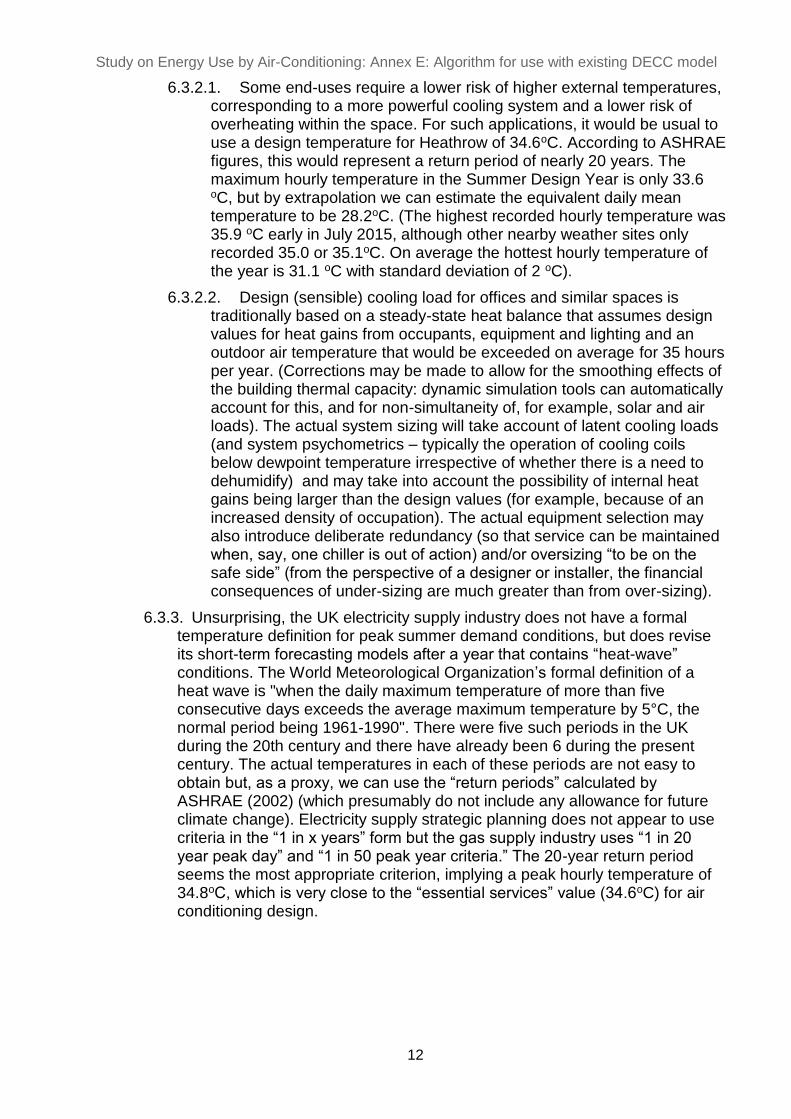
6.3.3. Unsurprising, the UK electricity supply industry does not have a formal temperature definition for peak summer demand conditions, but does revise its short-term forecasting models after a year that contains “heat-wave” conditions. The World Meteorological Organization’s formal definition of a heat wave is "when the daily maximum temperature of more than five consecutive days exceeds the average maximum temperature by 5°C, the normal period being 1961-1990". There were five such periods in the UK during the 20th century and there have already been 6 during the present century. The actual temperatures in each of these periods are not easy to obtain but, as a proxy, we can use the “return periods” calculated by ASHRAE (2002) (which presumably do not include any allowance for future climate change). Electricity supply strategic planning does not appear to use criteria in the “1 in x years” form but the gas supply industry uses “1 in 20 year peak day” and “1 in 50 peak year criteria.” The 20-year return period seems the most appropriate criterion, implying a peak hourly temperature of 34.8oC, which is very close to the “essential services” value (34.6oC) for air conditioning design.


13

Table 1: UK Hourly Peak Temperatures for the UK for Specified Average Return Intervals

6.4. Aggregated peak demands should preferably be based on observed aggregate

energy signatures (and, especially, residuals), as the hour to hour variability is

likely to be imperfectly correlated between individual buildings.

7. Examples of expected forms of air conditioning energy signatures 7.1. The following paragraphs illustrate why differences from the simple linear model

for air conditioning system energy signatures may be expected and their expected forms. Additional non-linearities may occur as the result of variations of cooling generator efficiency with temperature, or from the effect of (intentional or inadvertent) dehumidification.

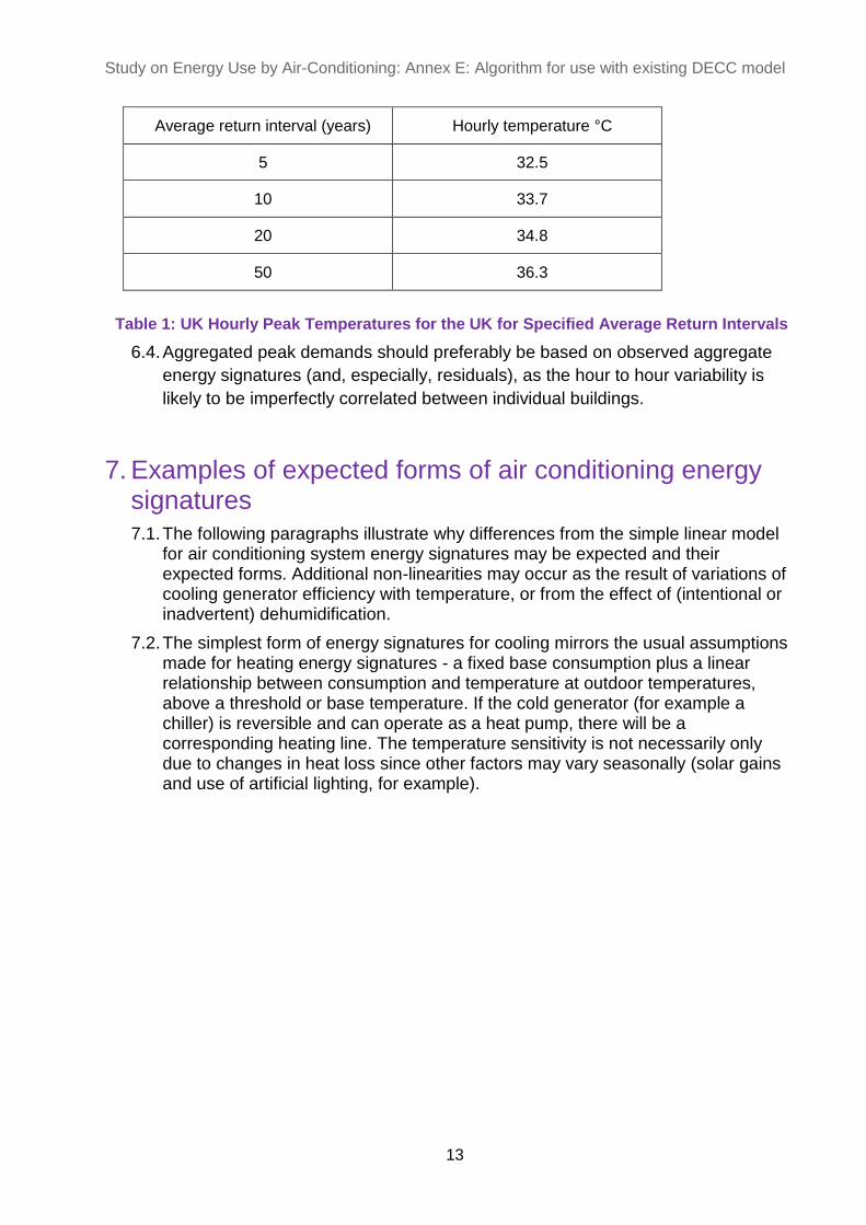
7.2. The simplest form of energy signatures for cooling mirrors the usual assumptions made for heating energy signatures - a fixed base consumption plus a linear relationship between consumption and temperature at outdoor temperatures, above a threshold or base temperature. If the cold generator (for example a chiller) is reversible and can operate as a heat pump, there will be a corresponding heating line. The temperature sensitivity is not necessarily only due to changes in heat loss since other factors may vary seasonally (solar gains and use of artificial lighting, for example).

Average return interval (years) Hourly temperature °C

5 32.5

10 33.7

20 34.8

50 36.3


14

0

5

10

15

20

1 3 5 7 9 11 13 15 17 19 21 23 25 27 29 31 33

me

an e

ne

rgy

de

man

d W

/m2

Outdoor temperature

Basic energy signatures

Heating Cooling

Figure 3 Basic electricity signature

7.2.1. There may (and should normally) be a “dead band” between the heating and cooling lines. From a control perspective it is often said that a 2oC dead-band is adequate to prevent the heating and cooling systems from competing with each other. For energy conservation, a range of 4 or 5oC (say 20oC and 24oC) between set-points is commonly recommended - which ought to be enough to prevent heating and cooling interactions.

7.2.2. Cooling generators such as chillers or room air conditioners often use electricity for controls, displays, crankcase heaters when they are “live” but not operating. These form part of the energy signature: although they may be small in terms of power, they may be present for far more hours than when the system is cooling.

7.2.3. Typical hours of operation for average European climate, from Ecodesign base case:

Off mode (cooling not in use) 5,087 hours

System “live” but not operating 3,673 hours, of which

Thermostat off 659 hours

Standby 1,377 hours

Crankcase heater operational 7,123 hours


15

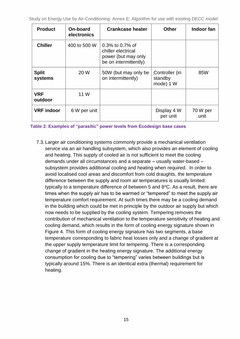
Product On-board electronics

Crankcase heater Other Indoor fan

Chiller 400 to 500 W 0.3% to 0.7% of chiller electrical power (but may only be on intermittently)

Split systems

20 W 50W (but may only be on intermittently)

Controller (in standby mode) 1 W

85W

VRF outdoor

11 W

VRF indoor 6 W per unit Display 4 W per unit

70 W per unit

Table 2: Examples of “parasitic” power levels from Ecodesign base cases

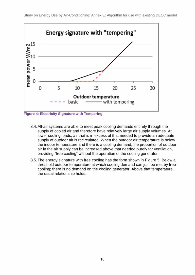
7.3. Larger air conditioning systems commonly provide a mechanical ventilation

service via an air handling subsystem, which also provides an element of cooling

and heating. This supply of cooled air is not sufficient to meet the cooling

demands under all circumstances and a separate – usually water-based –

subsystem provides additional cooling and heating when required. In order to

avoid localised cool areas and discomfort from cold draughts, the temperature

difference between the supply and room air temperatures is usually limited:

typically to a temperature difference of between 5 and 8oC. As a result, there are

times when the supply air has to be warmed or “tempered” to meet the supply air

temperature comfort requirement. At such times there may be a cooling demand

in the building which could be met in principle by the outdoor air supply but which

now needs to be supplied by the cooling system. Tempering removes the

contribution of mechanical ventilation to the temperature sensitivity of heating and

cooling demand, which results in the form of cooling energy signature shown in

Figure 4. This form of cooling energy signature has two segments, a base

temperature corresponding to fabric heat losses only and a change of gradient at

the upper supply temperature limit for tempering. There is a corresponding

change of gradient in the heating energy signature. The additional energy

consumption for cooling due to “tempering” varies between buildings but is

typically around 15%. There is an identical extra (thermal) requirement for

heating.


16

Figure 4: Electricity Signature with Tempering

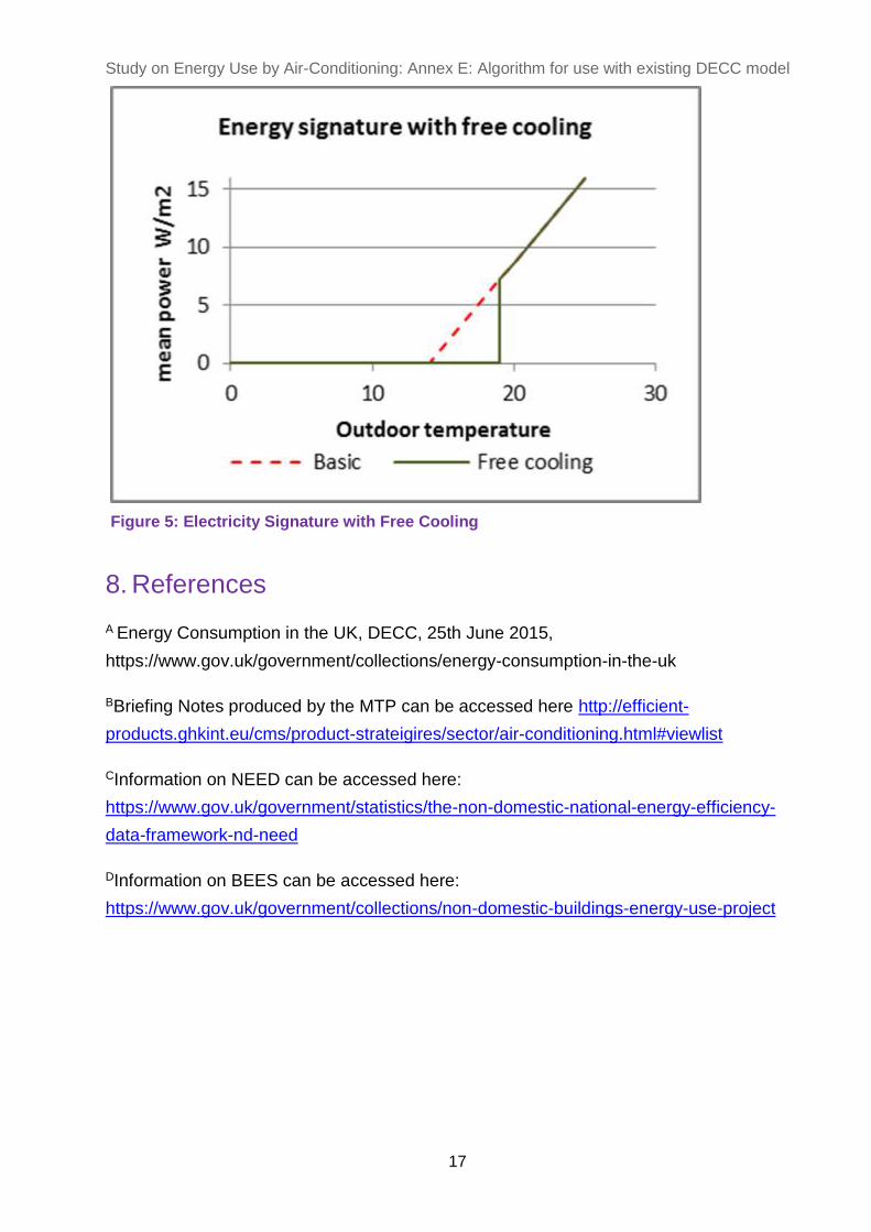
8.4. All-air systems are able to meet peak cooling demands entirely through the supply of cooled air and therefore have relatively large air supply volumes. At lower cooling loads, air that is in excess of that needed to provide an adequate supply of outdoor air is recirculated. When the outdoor air temperature is below the indoor temperature and there is a cooling demand, the proportion of outdoor air in the air supply can be increased above that needed purely for ventilation, providing “free cooling” without the operation of the cooling generator.

8.5. The energy signature with free cooling has the form shown in Figure 5. Below a threshold outdoor temperature at which cooling demand can just be met by free cooling; there is no demand on the cooling generator. Above that temperature the usual relationship holds.


17

Figure 5: Electricity Signature with Free Cooling

8. References

A Energy Consumption in the UK, DECC, 25th June 2015,

https://www.gov.uk/government/collections/energy-consumption-in-the-uk

BBriefing Notes produced by the MTP can be accessed here http://efficient-

products.ghkint.eu/cms/product-strateigires/sector/air-conditioning.html#viewlist

CInformation on NEED can be accessed here:

https://www.gov.uk/government/statistics/the-non-domestic-national-energy-efficiency-

data-framework-nd-need

DInformation on BEES can be accessed here:

https://www.gov.uk/government/collections/non-domestic-buildings-energy-use-project

http://efficient-products.ghkint.eu/cms/product-strateigires/sector/air-conditioning.html#viewlist

http://efficient-products.ghkint.eu/cms/product-strateigires/sector/air-conditioning.html#viewlist

https://www.gov.uk/government/statistics/the-non-domestic-national-energy-efficiency-data-framework-nd-need

https://www.gov.uk/government/statistics/the-non-domestic-national-energy-efficiency-data-framework-nd-need

https://www.gov.uk/government/collections/non-domestic-buildings-energy-use-project

Documents

Study on Energy Use by Air- Conditioning: Annex E ... · Study on Energy Use by Air-Conditioning: Annex E: Algorithm for use with existing DECC ... Algorithm for use with existing