PHYSICAL REVIEW B 101, 085125 (2020)

Study of the phase diagram of the Kitaev-Hubbard chain

Iman Mahyaeh and Eddy ArdonneDepartment of Physics, Stockholm University, SE-106 91 Stockholm, Sweden

(Received 14 November 2019; accepted 2 January 2020; published 14 February 2020)

We present a detailed study of the phase diagram of the Kitaev-Hubbard chain, that is the Kitaev chain in thepresence of a nearest-neighbor density-density interaction, using both analytical techniques as well as DMRG.In the case of a moderate attractive interaction, the model has the same phases as the noninteracting chain, atrivial and a topological phase. For repulsive interactions, the phase diagram is more interesting. Apart fromthe previously observed topological, incommensurate, and charge density wave phases, we identify the “excitedstate charge density wave” phase. In this phase, the ground state resembles an excited state of an ordinary chargedensity phase, but is lower in energy due to the frustrated nature of the model. We find that the dynamical criticalexponent takes the value z � 1.8. Interestingly, this phase only appears for even system sizes, and is sensitiveto the chemical potential on the edges of the chain. For the topological phase, we present an argument thatexcludes the presence of a strong zero mode for a large part of the topological phase. For the remaining region,we study the time dependence of the edge magnetization (using the bosonic incarnation of the model). Theseresults further expand the region where a strong zero mode does not occur.

DOI: 10.1103/PhysRevB.101.085125

I. INTRODUCTION

Topological phases of noninteracting fermions have beenstudied extensively and the full classification of the possiblephases has been found [1–4]. The classification scheme isbased on time-reversal symmetry, particle-hole symmetry, andchiral symmetry and which phases are possible depends on thespatial dimension. To a given class and spatial dimension onecan attribute a group, i.e., Z2 or Z, that describes the possiblegapped topological phases in that class. As an example theclass BDI has all three symmetries (squaring to one) and inone dimension its gapped phases are labeled by the group Z.The prototypical model belonging to this class is the Kitaevchain (with real couplings) [5]. In the topological phase of theKitaev chain, the model hosts Majorana zero modes on theedges of the chain. This zero mode results in a fully doublydegenerate many-body spectrum.

For interacting fermions there is no universal classificationscheme. Nonetheless for the class BDI it was shown that inthe presence of interactions the different topological classescorrespond to the elements of the group Z8 [6,7]. One shouldnote that this classification only concerns gapped phases andthe phase diagram of a general model has gapless points orregions as well. Therefore it is interesting not only to wonderabout how the interaction affects a topological phase [8] butalso how gapless phases emerge due to interactions.

The main aim of this paper is studying the phase diagramof the Kitaev chain in the presence of a density-densityinteraction, see Refs. [9–14] for earlier results for this model.

Published by the American Physical Society under the terms of theCreative Commons Attribution 4.0 International license. Furtherdistribution of this work must maintain attribution to the author(s)and the published article’s title, journal citation, and DOI. Fundedby Bibsam.

We refer to this model as the Kitaev-Hubbard chain. Westudy both the attractive and repulsive regime. In addition tothe trivial and topological phases which are inherited fromthe Kitaev chain, the model has an incommensurate phase, acharge density wave phase, and a new phase which is sensitiveto the system size and the chemical potential at the boundariesof the chain. Moreover, we study the possibility of having afull doubly degenerate many-body spectrum in the topologicalphase of this interacting model.

The paper is organized as follows. In Sec. II we brieflyreview both the classical and quantum axial next-nearest-neighbor Ising (ANNNI) model and present the model ofinterest for this paper, namely the Kitaev-Hubbard chain.We show that the quantum ANNNI model and the Kitaev-Hubbard chain are dual to each other and present the mainresult, that is the phase diagram of this model. We continueby presenting our analytical results based on bosonization andthe numerical results based on density matrix renormalizationgroup (DMRG) [15,16] for an attractive interaction in Sec. III.In Sec. IV we move on to the repulsive regime, for whichthere is an incommensurate phase and a new phase which wasmissed previously. Moreover, we will discuss the properties ofthe highest excited states as well as the finite temperature fea-tures of the model in Sec. V. We conclude the paper in Sec. VI.

II. THE MODEL AND THE PHASE DIAGRAM

To introduce the model we set the scene by reminding thereader of the classical Ising model, which is the cornerstoneof our understanding of phase transitions [17–20].

To define this model consider a square lattice where oneach site, with coordinate (i, j), one has a classical spin,si, j = ±1. For a configuration of spins {s} the energy is

E [{s}] = −∑i, j

(J̃1si, j si+1, j + J̃⊥si, j si, j+1). (1)

2469-9950/2020/101(8)/085125(14) 085125-1 Published by the American Physical Society

IMAN MAHYAEH AND EDDY ARDONNE PHYSICAL REVIEW B 101, 085125 (2020)

We assume that J̃1, J̃⊥ > 0. The classical Ising model in twodimensions was initially solved by Onsager [17], later othersolutions were found, see [18]. The model has two phases. Fortemperatures T less than the critical temperature Tc, it is inthe ferromagnetic phase and for T > Tc it is in the disorderedphase.

As a generalization one can consider the ANNNI modelwhere one adds an extra interaction along one axis, whichcould favor ferromagnetic or antiferromagnetic alignment[9,21,22]. The energy for a given configuration of spins of theANNNI model is

E [{s}] = −∑i, j

(J̃1si, j si+1, j + J̃2si, j si+2, j )

−∑i, j

J̃⊥si, j si, j+1. (2)

We follow the usual notation and define κ̃ = − J̃2

J̃1. For κ̃ <

0 there is no frustration, and the axial term only modifies thecritical temperature. For κ̃ > 0, however, the situation is moresubtle. For small and positive κ̃ the model has two phases,a ferromagnetic and paramagnetic phase. The point κ̃ = 1/2is a multicritical point, where four phases meet, namely theferromagnet, paramagnet, a floating phase, and the so-called“antiphase” [9]. In the antiphase, the axial interaction dom-inates and there are four spin configurations that minimizethe energy. For the floating phase however, all interactions areimportant. Whether the floating phase continues to infinite κ̃

is an open question, which we study in this paper by analyzingthe corresponding quantum model.

The quantum counterpart of the classical Ising model isthe transverse field Ising model (TFIM) [23–25]. This modelis defined on a chain. On each site there is a spin-1/2 degreeof freedom and the Hamiltonian for a chain of size L can bewritten as

H = −J1

L−1∑j=1

τ zj τ

zj+1 + B

L∑j=1

τ xj , (3)

where τα are Pauli matrices. One can relate the parametersJ1 and B in terms of coupling constants of the classicalmodel and the temperature [25]. The TFIM shows a quantumphase transition at T = 0. For |B| < |J1| the model is in theferromagnetic phase while for |B| > |J1| it is in the disorderedphase. The classical Ising model in two dimensions and theone-dimensional TFIM are in the same universality class.

The quantum ANNNI model was also studied [10–12,14].The Hamiltonian reads [9]

H = −J1

L−1∑j=1

τ zj τ

zj+1 − J2

L−2∑j=1

τ zj τ

zj+2 + B

L∑j=1

τ xj . (4)

In analogy with the classical ANNNI model, we define κ =− J2

J1. For κ < 1

2 the model has only ferromagnetic and param-agnetic phases. In this regime there is a second order phasetransition between the ordered and the disordered phase atBc(κ ). The point κ = 1

2 is a multicritical point from which thefloating phase emerges. For very large κ the dominant termis the next-nearest-neighbor term in Eq. (4) which gives riseto four ground states. Previous studies found that the floating

phase survives till κ � 5 [11,12]. We will present our resultsfor infinite κ by studying the dual model.

To study large frustration, κ � 1, we employ the dualitymap as follows:

τ zj τ

zj+1 → σ z

j ,

τ xj → σ z

j σzj+1. (5)

We further perform an on-site rotation,

σ xj → σ z

j , σ zj → (−1) jσ x

j . (6)

Using these two transformations one can transform the Hamil-tonian for the quantum ANNNI model, Eq. (4), to an interact-ing quantum Ising model,

H = −BL−1∑j=1

σ xj σ

xj+1 − J1

L∑j=1

σ zj + J2

L−1∑j=1

σ zj σ

zj+1. (7)

Note that the sign of B and J1 are not important and wewill assume that both are positive. The sign of J2, however,is crucial. Hence we use B as our energy scale and study thefollowing Hamiltonian:

H (h,U ) = −L−1∑j=1

σ xj σ

xj+1 − h

L∑j=1

σ zj + U

L−1∑j=1

σ zj σ

zj+1, (8)

in which,

h = J1

B, U = κ

J1

B= κh. (9)

By performing a Jordan-Wigner (JW) transformation [26],one arrives at the Kitaev-Hubbard chain,

H (h,U ) = −L−1∑j=1

(c†j − c j )(c

†j+1 + c j+1)

− hL∑

j=1

(1 − 2c†j c j )

+ UL−1∑j=1

(1 − 2c†j c j )(1 − 2c†

j+1c j+1). (10)

For U = 0, the model reduces to the TFIM (or the Kitaevchain [5]) which is exactly solvable [24,27]. In the bosonicrepresentation the two phases are the ordered (h < 1) and thedisordered (h > 1) phases which are converted to the topo-logical and the trivial phases, respectively, in the fermionicincarnation. The phase transition between these phases isdescribed by the c = 1

2 Ising CFT.In the topological phase the model hosts Majorana zero

modes which live on the edges and has zero energy up toexponentially small corrections in the system size. An inter-esting question is whether the topological phase is stable inthe presence of interactions [8,28]. The U term in Eq. (8) givesrise to a density-density interaction, but renders the modelnonintegrable.

Another special case is h = 0 for which the model iscalled the XY model [27]. This model is gapped, exceptwhen U = ±1, which are critical points with central chargec = 1. The gapped phases are ordered phases in the bosonicrepresentation and topological in the fermionic incarnation.

085125-2

STUDY OF THE PHASE DIAGRAM OF THE … PHYSICAL REVIEW B 101, 085125 (2020)

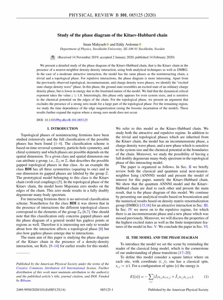
TopologicalTrivial

IC

CDW

−1.0 −0.5 0.0 0.5 1.0 1.5U

0.2

0.4

0.6

0.8

1.0

1.2h

FIG. 1. The phase diagram for the model in Eq. (8). The greenregion, between the IC and CDW phase, is the esCDW phase.

It is worth to mention that the model in Eq. (8) is actuallyrelevant for an array of superconducting islands [29]. More-over, for a specific set of couplings known as the Peschel-Emery (PE) line, the ground state is exactly doubly degenerate[30]. This line lies in the topological phase and host weak zeromodes [31,32], see Sec. V for more detail on this.

We obtained the phase diagram of the model in Eq. (8)as presented in Fig. 1. Parts of this phase diagram wereschematically drawn previously based on the known resultsfor the quantum ANNNI model [10,11,13,28,29]. We believe,however, that in the previous studies one phase (the greenregion in the plot) has been missed. This phase will bedescribed in Sec. IV C.

III. THE ATTRACTIVE INTERACTION CASE

For attractive interactions, U < 0, there is no frustration,κ < 0, and one expects a direct transition from the topologicalphase (ordered phase) to the trivial phase (disordered phase),as is the case for U = 0. To study the U < 0 case, one canstart from the Ising critical point, namely h = 1 and U = 0,and perform perturbative calculations to find the location ofthe phase transition [33]. We will, however, start from anothercritical point, namely the XY critical point with h = 0 andU = −1. Close to this point we can use bosonization. To doso it is convenient to transform the Hamiltonian in Eq. (8). Wefirst do an on-site rotation,

σ xj → (−1) jσ

yj , σ z

j → (−1) jσ xj , (11)

which changes the Hamiltonian to

H (h,U ) =∑

j

(σ x

j σxj+1 + σ

yj σ

yj+1

)

+∑

j

[−δUσ xj σ

xj+1 − h(−1) jσ x

j

], (12)

in which we defined δU = U + 1 and dropped the lower andupper bounds of the sums, since we will be working in thecontinuum limit. We assume that δU, h � 1.

We can use the JW transformation, write the Hamiltonianin terms of spinless fermions ψ j , and perform a Fouriertransformation to work in momentum space. Doing so, the

first two terms, namely the XY model, give rise to a gaplesscos(k) band, which can be linearized around k = ±π

2 , to getthe continuum model,

ψ j = √a[ei π

2 jψ+(x) + e−i π2 jψ−(x)

]. (13)

In the last equation a is the lattice spacing and x = ja will bethe continuous spatial coordinate.

We first consider the δU term in Eq. (12). Plugging Eq. (13)into this term we get a term proportional to∫

(ψ†+(x)ψ†

−(x) + ψ+(x)ψ−(x))dx. (14)

To further simplify the result, we use the dual fields φ(x)and θ (x), which obey the commutator [φ(x), θ (y)] = i�(y −x), where �(x) is the Heaviside step function. Therefore,∂xθ (x) is the conjugate momentum of the field φ(x). Weemploy the bosonization dictionary [34],

ψ±(x) = 1√2πα

ei√

π [±φ(x)−θ (x)] , (15)

in which α is a cutoff in momentum space. Hence we canwrite the δU term in terms of the dual fields, which is propor-tional to ∫

cos(√

4πθ )dx. (16)

The h term in Eq. (12) can be treated in the same way.Using the bosonization dictionary and by dropping the fastoscillatory terms which are proportional to (−1) j , one canshow that

(−1) jσ−j → e−i

√πθ (x). (17)

Therefore the h term reduces to∫cos(

√πθ )dx. (18)

The full Bosonized Hamiltonian then reads

H (h, 1 + δU ) = H0 + c1δU∫

cos(√

4πθ )dx

+ c2h∫

cos(√

πθ )dx, (19)

in which H0 is the free bosonic Hamiltonian and c1 and c2

are some constants which depend on a and α. Since H0 isquadratic, we can calculate the renormalization group flow ofthe couplings, δ and h, up to first order

dδU

dl= δU, (20)

dh

dl= 7

4h. (21)

We should mention that we assumed that we can drop therenormalization of K , one of the Luttinger parameters. Thesetwo equations tell us that close to the XY point, h = 0 andU = −1, the curve separating the topological and the trivialphases is given by

h ∼ (U + 1)7/4. (22)

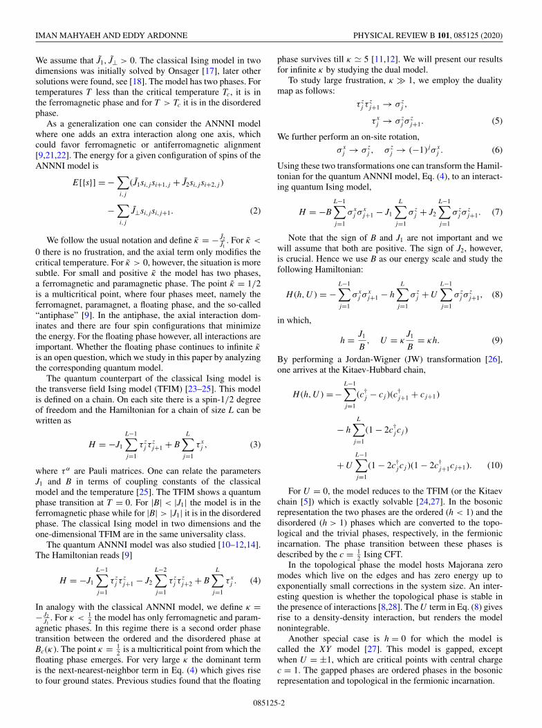
To check this analytical result we performed a numericalstudy and compared to the results shown in Fig. 2. To locate

085125-3

IMAN MAHYAEH AND EDDY ARDONNE PHYSICAL REVIEW B 101, 085125 (2020)

FIG. 2. The phase boundary between the trivial band insulatorand the topological phase. The blue line is hc(U ) = 0.99(U + 1)1.73.The red line is hc(U ) = 0.97(U + 1)7/4.

the phase transition we ran DMRG using the ALPS libraries[35–37]. This DMRG study also serves to get acquainted withthe performance of the algorithm for the model at hand.

We should note that the second term in Eq. (10) [themagnetic field in the bosonic incarnation in Eq. (8)] has beenimplemented as follows:

L−1∑j=1

−h

2[(1 − 2c†

j c j ) + (1 − 2c†j+1c j+1)]. (23)

Therefore in the bosonic incarnation the strength of the mag-netic field in the bulk is h while it is half of this strength onthe first and the last sites, h1 = hL = h

2 .We used finite size scaling (FSS) to pinpoint the transition.

Within this framework, one finds the ground state and thefirst excited state and use the following scaling ansatz for theenergy difference between them, δ, close to the critical point[38],

δ(L, h) = L−zF[L−ν (h − hc)], (24)

where L is the system size, z is the dynamical critical expo-nent, ν is the correlation length exponent, and F is a scalingfunction. For the TFIM it is known that z = ν = 1 [39].

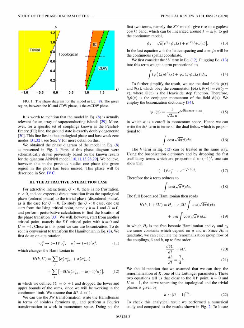
We present our data for U = −0.4 as an example. For agiven U at h = hc(U ), the quantity Lzδ does not depend onthe system size. In Fig. 3 it is clear that Lδ for different systemsizes cross at hc = 0.406. One can use this critical value andtake ν = 1 to check the validity of the ansatz Eq. (24), seeFig. 3. Indeed, the data for different system sizes follow thesame functional form if one scales the h axis appropriately.

We used FSS for −0.8 � U � 0.25 and calculated thecritical field hc(U ). The data are presented in Fig. 2. We fitteda power law with the form

hc(U ) = a(U + 1)b (25)

to the data. Using the data in the range of −0.8 � U � −0.5the fitting gives a = 1.02 and b = 1.81. For the full range ofdata in Fig. 2, however, the best power-law fit has a = 0.99and b = 1.73. The blue line in Fig. 2 is the fit to the full set ofdata points. These results are in a very good agreement withour bosonization result in Eq. (22). Our results are also in very

FIG. 3. Finite size scaling for U = −0.4. The quantity Lδ =L(E1 − E0) for different system sizes cross at h = 0.406.

good agreement with the perturbative approach of Ref. [33]around the point h = 1, U = 0.

To determine the central charge c along the curve we usedthe scaling of the excited states’ energy as a function of systemsize L [40] and the Calabrese-Cardy (CC) formula for theentanglement entropy (EE) of a subsystem of size l , in thecase of an open chain at the critical point S(l, L) [41–43],

S(l ) = c

6log

[L sin

(π l

L

)]+ S0. (26)

Here c is the central charge and S0 is a constant. Both methodsresult in the central charge c = 1

2 . Therefore we have thecentral charge c = 1

2 all along the transition line except forh = 0 and U = −1, where we have the XY critical point withcentral charge c = 1 [40].

IV. THE REPULSIVE INTERACTION CASE

In this section we study the Hamiltonian Eq. (8) withrepulsive interaction U > 0, which is more involved. We canqualitatively understand the physics in the weak and stronginteraction limits. For weak interaction, U � 1, we still ex-pect to have two phases, i.e., a topological (ordered) phaseand a trivial (disordered) phase, as in the case of the TFIM.On the other hand for very strong interaction, the model is inthe Néel phase which corresponds to the charge density wave(CDW) in the fermionic representation. Apart from these twoeasy limits it is hard to say something about the phase(s)for intermediate interaction strength. For the earlier studiesof the model with repulsive interaction using DMRG andbosonization we refer to Refs. [10–12,14].

To find the phase diagram of the model we performedDMRG using the ALPS libraries [35–37]. We used thefermionic incarnation of the model, i.e., Eq. (10), to performthe DMRG. This is useful since the total parity P is a con-served quantity,

P =L∏

j=1

σ zj =

L∏j=1

(1 − 2n j ). (27)

085125-4

STUDY OF THE PHASE DIAGRAM OF THE … PHYSICAL REVIEW B 101, 085125 (2020)

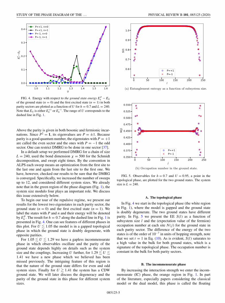
FIG. 4. Energy with respect to the ground state energy EPn − EG

of the ground state (n = 0) and the first excited state (n = 1) in bothparity sectors are plotted as a function of U for h = 0.7 and L = 240.Note that EG is either E+1

0 or E−10 . The range of U corresponds to the

dashed line in Fig. 1.

Above the parity is given in both bosonic and fermionic incar-nations. Since P2 = 1, its eigenvalues are P = ±1. Becauseparity is a good quantum number, the eigenstates with P = +1are called the even sector and the ones with P = −1 the oddsector. One can restrict DMRG to be done in one sector [37].

In a default setup we performed DMRG for a chain of sizeL = 240, used the bond dimension χ = 500 for the Schmidtdecomposition, and swept eight times. By the convention inALPS each sweep means an optimization from the first site tothe last one and again from the last site to the first one. Wehave, however, checked our results to be sure that the DMRGis converged. Specifically, we increased the number of sweepsup to 12, and considered different system sizes. We alreadynote that in the green region of the phase diagram (Fig. 1), thesystem size modulo four plays an important role. We discussthis issue extensively below.

To begin our tour of the repulsive regime, we present ourresults for the lowest two eigenstates in each parity sector, theground state (n = 0) and the first excited state (n = 1). Welabel the states with P and n and their energy will be denotedby EP

n . The result for h = 0.7 along the dashed line in Fig. 1 ispresented in Fig. 4. One can see features of different phases inthis plot. For U � 1.05 the model is in a gapped topologicalphase in which the ground state is doubly degenerate, withopposite parities.

For 1.05 � U � 1.29 we have a gapless incommensuratephase in which observables oscillate and the parity of theground state depends highly on details such as the systemsize and the couplings. Increasing U further, for 1.29 � U �1.41 we have a new phase which we believed has beenmissed previously. The intriguing feature of this region isthat the nature of the ground state differs for even and oddsystem sizes. Finally for U � 1.41 the system has a CDWground state. We will later discuss the degeneracy and theparity of the ground state in this phase for different systemsizes.

(a) Entanglement entropy as a function of subsystem size.

(b) Occupation number in the ground state.

FIG. 5. Observables for h = 0.7 and U = 0.95, a point in thetopological phase, are plotted for the two ground states. The systemsize is L = 240.

A. The topological phase

In Fig. 4 we start in the topological phase (the white regionin Fig. 1), where the model is gapped and the ground stateis doubly degenerate. The two ground states have differentparity. In Fig. 5 we present the EE S(l ) as a function ofsubsystem size l and the (expectation value of the fermion)occupation number at each site N ( j) for the ground state ineach parity sector. The difference of the energy of the twostates is of the order of 10−7 in units of hopping strength, notethat we set t = 1 in Eq. (10). As is evident, S(l ) saturates toa high value in the bulk for both ground states, which is asignature of the topological phase. The occupation number isconstant in the bulk for both parity sectors.

B. The incommensurate phase

By increasing the interaction strength we enter the incom-mensurate (IC) phase, the orange region in Fig. 1. In partof the literature, especially papers considering the classicalmodel or the dual model, this phase is called the floating

085125-5

IMAN MAHYAEH AND EDDY ARDONNE PHYSICAL REVIEW B 101, 085125 (2020)

(a) Entanglement entropy as a function of subsystem size.

(b) Occupation number in the ground state.

FIG. 6. Ground state observables for h = 0.7 and U = 1.2, apoint in the incommensurate phase, are plotted for L = 240. Theground belongs to the odd sector.

phase. In this phase the ground state is unique but its paritydoes strongly depend on the parameters and the system size.

In Fig. 6 we present the EE and occupation number N ( j)for a chain of size L = 240 at a point in the IC phase, h =0.7 and U = 1.2. For this set of parameters the ground statehappens to belong to the odd sector.

One signature of this phase is the presence of oscillations inthe EE and occupation number. Another feature of this phaseis that one can use the CC formula, Eq. (26), for the EE tofit the data. Previously this has been done to distinguish theIC phase from the topological and the trivial phases of a Z3

parafermionic chain [44].For fitting we usually drop the first and the last 20 sites

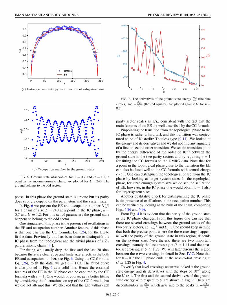
because there are clear edge and finite size effects in the bothEE and occupation number, see Fig. 6. Using the CC formula,Eq. (26), to fit the data, we get c = 1.03. The fitted curveis also plotted in Fig. 6 as a solid line. Hence the essentialfeatures of the EE in the IC phase can be captured by the CCformula with c = 1. One would, of course, get a better fittingby considering the fluctuations on top of the CC formula, butwe did not attempt this. We checked that the gap within each

FIG. 7. The derivatives of the ground state energy ∂EG∂U (the blue

circles) and − ∂2EG∂U 2 (the red squares) are plotted against U for h =

0.7.

parity sector scales as 1/L, consistent with the fact that themain features of the EE are well described by the CC formula.

Pinpointing the transition from the topological phase to theIC phase is rather a hard task and this transition was conjec-tured to be of Kosterlitz-Thouless type [9,11]. We looked atthe energy and its derivatives and we did not find any signatureof a first or second order transition. We set the transition pointby the energy difference of the order of 10−3 between theground state in the two parity sectors and by requiring c = 1for fitting the CC formula to the DMRG data. Note that fora point in the topological phase close to the transition the EEcan also be fitted well to the CC formula with central chargec < 1. One can distinguish the topological phase from the ICphase by looking at larger system sizes. In the topologicalphase, for large enough system size we do see the saturationof EE, however, in the IC phase one would obtain c = 1 alsofor larger system sizes.

Another qualitative check for distinguishing the IC phaseis the presence of oscillations in the occupation number. Thiscan be verified by looking at the bulk of the chain, comparingFigs. 5(b) and 6(b).

From Fig. 4 it is evident that the parity of the ground statein the IC phase changes. From this figure one can see thatthere are several crossings between the ground states of thetwo parity sectors, i.e., E+1

0 and E−10 . One should keep in mind

that both the precise point where the these crossings happen,as well the parity of the ground state in this region, dependson the system size. Nevertheless, there are two importantcrossings, namely the last crossing at U � 1.41 and the next-to-last crossing at U � 1.28. We will later discuss the regionbetween these two crossings in detail in Sec. IV C. Note thatfor h = 0.7 the IC phase ends at the next-to-last crossing atU � 1.28 in Fig. 4.

To verify that level crossings occur we looked at the groundstate energy and its derivatives with the steps of 10−2 alongthe U axis. The first and the second derivatives of the groundstate energy with respect to U are shown in Fig. 7. There arediscontinuities in ∂EG

∂U which give rise to the peaks in − ∂2EG∂U 2 .

085125-6

STUDY OF THE PHASE DIAGRAM OF THE … PHYSICAL REVIEW B 101, 085125 (2020)

(a) Energy with respect to the ground state energy, EPn − EG, of

the ground state (n = 0) and the first excited state (n = 1) inboth parity sectors are plotted as function of U for h = 0.05.

(b) The derivatives of the ground state energy, ∂EG∂U

(the blue

circles) and − ∂2EG∂U2 (the red squares) for h = 0.1 are plotted.

FIG. 8. Energy levels and the derivatives of the ground stateenergy for small h are plotted. The system size is L = 240.

We have looked at the similar quantities for different systemsizes and the discontinuities are always present in the firstorder derivative. These are clear signatures of level crossings.We note that both the number of crossings, as well as theirlocation, depends rather strongly on the system size.

To address the question about the presence of the floatingphase in the ANNNI model [Eq. (4)] in the highly frus-trated limit, i.e., κ � 1, we can use our knowledge of theKitaev-Hubbard chain. Because the Kitaev-Hubbard chain isdual to the ANNNI model, the presence of the IC phase inthe fermionic incarnation corresponds to the presence of thefloating phase in the ANNNI model.

From Eq. (9) we can see that for U � 1 and small h,we will be in the regime of B

J1, κ � 1, which is exactly the

regime where the presence of the floating phase in the ANNNImodel was under debate. In Fig. 8(a) we plot the energy of theground state (n = 0) and the first excited state (n = 1) in bothparity sectors for a chain of length L = 240, at h = 0.05. This

corresponds to κ � 20. The situation is similar to h = 0.7,as plotted in Fig. 4. For low enough U the ground state isdoubly degenerate and the states have different parities, i.e., atopological phase. For large enough U , the ground state is alsodegenerate and the states have the same parity, i.e., P = +1 inthis case.

In Fig. 8(b) one observes a discontinuity in ∂EG∂U and the

corresponding peak in − ∂2EG∂U 2 for h = 0.1 (which corresponds

to κ = 10) at U = 1.05, as well as a broad feature at U =0.99. In addition, it is also possible to fit the EE with the CCformula, resulting in c = 1 for a small region in U , even forh = 0.05. Finally, one observes an onset to the oscillationsin the occupation number, that is characteristic for the ICphase. Given these features, we conclude that the IC phase inthe Kitaev-Hubbard chain continues down to the XY criticalpoint. Therefore, we also conclude that the floating phase inthe ANNNI model is present for arbitrarily large frustration.

C. The excited-state CDW phase

In our numerical studies we found that the ground state forh = 0.7 and U � 1.41 has CDW order and a low EE, which isconstant in the bulk, that is, independent of the subsystem size.By looking at the energy levels in Fig. 4 we see that there is aregion, 1.28 � U � 1.41, just before the CDW phase in whichthe the ground state is in the odd sector for our default systemsize, L = 240. We believe that this part of the phase diagram,colored light green in Fig. 1, is a phase which had beenmissed before and has been considered to be part of the CDW.We will discuss the properties of this phase thoroughly andshow how the behavior of the model in this part of the phasediagram depends on the system size. Moreover, we show thatthe transition point from the new phase to the CDW phase canbe actually controlled by tuning the chemical potential on thefirst and the last sites.

We present the EE and occupation number for a genericpoint (h = 0.7 and U = 1.325) in the new phase in Fig. 9.It is clear the EE of the ground state grows as a function ofsubsystem size. The particle number has a long wavelengthoscillation of twice the system size, accompanied by a π phaseshift for neighboring sites. These observations show that theground state does not have a conventional CDW ordering forour system size. In fact, the properties of the ground state re-semble the properties of low-lying excited states in the CDWphase. We therefore refer to this phase as the “excited-statecharge density wave” (esCDW) phase. In addition, we foundthat the model is gapless by looking at the first (n = 1) and thesecond (n = 2) excited states in the odd sector. The energydifference between them, �E−1

n = E−1n − E−1

0 , approacheszero as L−1.80 for n = 1, 2. The data for n = 1 and the fit areshown in Fig. 10. This shows this phase is a gapless phase withthe dynamical critical exponent z � 1.80 and hence cannot bedescribed by a conformal field theory. We also found that thereis a finite gap to the lowest energy state in the even sector. InFig. 11 we plot E+1

0 − E−10 as a function 1

L which shows theexistence of the gap.

An intriguing feature of this region of the phase diagramis that its features depend crucially on the system size. Theground state belongs to the odd sector for system sizes thatare a multiple of four, L = 4n. For L = 4n + 2 however, the

085125-7

IMAN MAHYAEH AND EDDY ARDONNE PHYSICAL REVIEW B 101, 085125 (2020)

(a) Entanglement entropy as a function of subsystem size.

(b) Occupation number.

FIG. 9. Observables for the ground state at h = 0.7 and U =1.325, a point in the esCDW phase are plotted. The system size isL = 240.

ground state shows the same behavior as described above, butit belongs to the even sector.

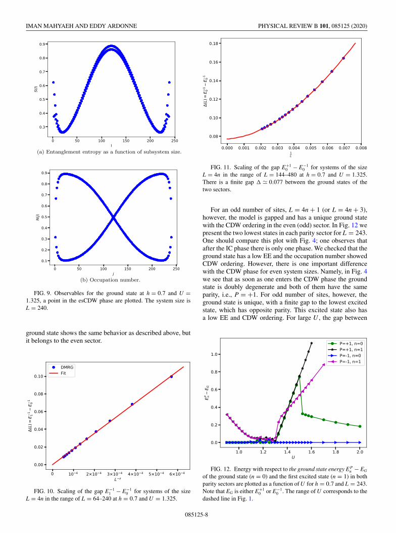
FIG. 10. Scaling of the gap E−11 − E−1

0 for systems of the sizeL = 4n in the range of L = 64–240 at h = 0.7 and U = 1.325.

FIG. 11. Scaling of the gap E+10 − E−1

0 for systems of the sizeL = 4n in the range of L = 144–480 at h = 0.7 and U = 1.325.There is a finite gap � � 0.077 between the ground states of thetwo sectors.

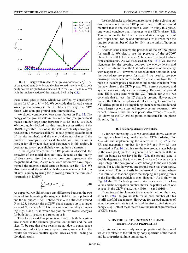
For an odd number of sites, L = 4n + 1 (or L = 4n + 3),however, the model is gapped and has a unique ground statewith the CDW ordering in the even (odd) sector. In Fig. 12 wepresent the two lowest states in each parity sector for L = 243.One should compare this plot with Fig. 4; one observes thatafter the IC phase there is only one phase. We checked that theground state has a low EE and the occupation number showedCDW ordering. However, there is one important differencewith the CDW phase for even system sizes. Namely, in Fig. 4we see that as soon as one enters the CDW phase the groundstate is doubly degenerate and both of them have the sameparity, i.e., P = +1. For odd number of sites, however, theground state is unique, with a finite gap to the lowest excitedstate, which has opposite parity. This excited state also hasa low EE and CDW ordering. For large U , the gap between

FIG. 12. Energy with respect to the ground state energy EPn − EG

of the ground state (n = 0) and the first excited state (n = 1) in bothparity sectors are plotted as a function of U for h = 0.7 and L = 243.Note that EG is either E+1

0 or E−10 . The range of U corresponds to the

dashed line in Fig. 1.

085125-8

STUDY OF THE PHASE DIAGRAM OF THE … PHYSICAL REVIEW B 101, 085125 (2020)

FIG. 13. Energy with respect to the ground state energy EPn − EG

of the ground state (n = 0) and the first excited state (n = 1) in bothparity sectors are plotted as a function of U for h = 0.7 and L = 240with the implementation of the magnetic field in Eq. (28).

these states goes to zero, which we verified by consideringvalues for U up to U ∼ 10. We conclude that for odd systemsizes, upon increasing U , the IC phase gives way to a CDWphase (with a unique ground state) immediately.

We should comment on one more feature in Fig. 12. Theenergy of the ground state in the even sector (the green dots)makes a rather large jump between U = 1.5 and U = 1.525.We thoroughly checked that this jump is not an artifact of theDMRG algorithm. First of all, the states are clearly converged,because the observables all have smooth profiles (as a functionof the site number), and the energy does not change if thenumber of sweeps is increased. In addition, this feature ispresent for all system sizes and parameters in this region, itdoes not go away upon slightly varying these parameters.

In the region where the esCDW phase is observed, thebehavior of the model does not only depend on the (parityof the) system size, but also on how one implements themagnetic field term. As we mentioned before we have imple-mented the magnetic field term on bonds, see Eq. (23). Wealso considered the model with the same magnetic field onall sites, namely by using the following term in the fermionicincarnation in DMRG:

L∑j=1

−h(1 − 2c†j c j ). (28)

As expected, we did not seen any difference between the twoways of implementing the magnetic field in the topologicaland the IC phases. The IC phase for h = 0.7 still ends aroundU � 1.28, however, the esCDW phase extends up to a largervalue of U , namely U � 1.68, as can be observed by compar-ing Figs. 4 and 13, in which we plot the two lowest energiesfor both parity sectors as a function of U .

Therefore the esCDW phase is sensitive to both the systemsize as well as the chemical potential on the first and the lastsites. To be sure that these results are not due to convergenceissues and unluckily chosen system sizes, we checked theresults for various smaller system sizes as well, leading toidentical results.

We should make two important remarks, before closing ourdiscussion about the esCDW phase. First of all we shouldmention that if one uses infinite DMRG to study this phase,one would conclude that it belongs to the CDW phase [12].This is due to the fact that the ground state energy per unitsite (or per bond) for the odd number of sites is lower than theone for even number of sites by 10−3 in the units of hoppingenergy.

Another issue concerns the presence of the esCDW phasefor small h. We clearly see the presence of the esCDWphase for h = 0.1. For smaller h, however, it is hard to drawfirm conclusions. As we discussed in Sec. IV B we see thesignatures for the crossing between the energy levels andhence discontinuities in the first order derivative of the energywith respect to U . However, to conclude that both the IC andthe new phase are present for small h we need to see twocrossings, one which corresponds to the transition from the ICphase to the new phase and another one for the transition fromthe new phase to the CDW phase. With current accuracy andsystem sizes we only see one crossing. Because the groundstate EE is consistent with the CC formula for c = 1 weconclude that at least the IC phase is present. However, thethe width of these two phases shrinks as we get closer to theXY critical point and distinguishing them becomes harder andneeds larger system sizes and more accurate treatments. Weexpect, however, that the new phase also extends to h = 0,i.e., down to the XY critical point, as indicated in the phasediagram, Fig. 1.

D. The charge density wave phase

By further increasing U , as we concluded above, we enterthe regime where the ground state has CDW ordering. ForL = 240 and implementing the h term as in Eq. (23), theEE and occupation number for h = 0.7 and U = 1.5, arepresented in Fig. 14. In this case the two ground states belongto the even parity sector. In general, if we implement the hterm on bonds as we have in Eq. (23), the ground state isdoubly degenerate. For L = 4n (or L = 4n + 2), where n is alarge integer, the two ground states belongs to the even (odd)sector. For L odd, however, one ground state has even parity,the other odd. This can easily be understood in the limit whereU is infinite, so that one ignore the hopping and pairing termsin the Hamiltonian (which is then diagonal). As is shown inFig. 14 the EE for both ground states is saturated to a lowvalue and the occupation number shows the pattern which oneexpects in the CDW phase, i.e., (1010 · · · ) and (0101 · · · ).

If one instead implements the magnetic field on the sites,as in Eq. (28), the ground state for an even number of sitesis still twofold degenerate. However, for an odd number ofsites, the ground state is unique, and the first excited state hasenergy 2|h|. Both of these states have the usual characteristicsof CDW states.

V. ON THE EXCITED STATES AND FINITETEMPERATURE PROPERTIES

In this section we study some properties of the modelwhich are related to the full many-body spectrum of the modeland its properties at finite temperature.

085125-9

IMAN MAHYAEH AND EDDY ARDONNE PHYSICAL REVIEW B 101, 085125 (2020)

(a) Entanglement entropy as a function of subsystem size.

(b) Occupation number.

FIG. 14. Observables for the ground state (n = 0) and the firstexcited state (n = 1) at h = 0.7 and U = 1.5, a point in the CDWphase, are plotted. The system size is L = 240.

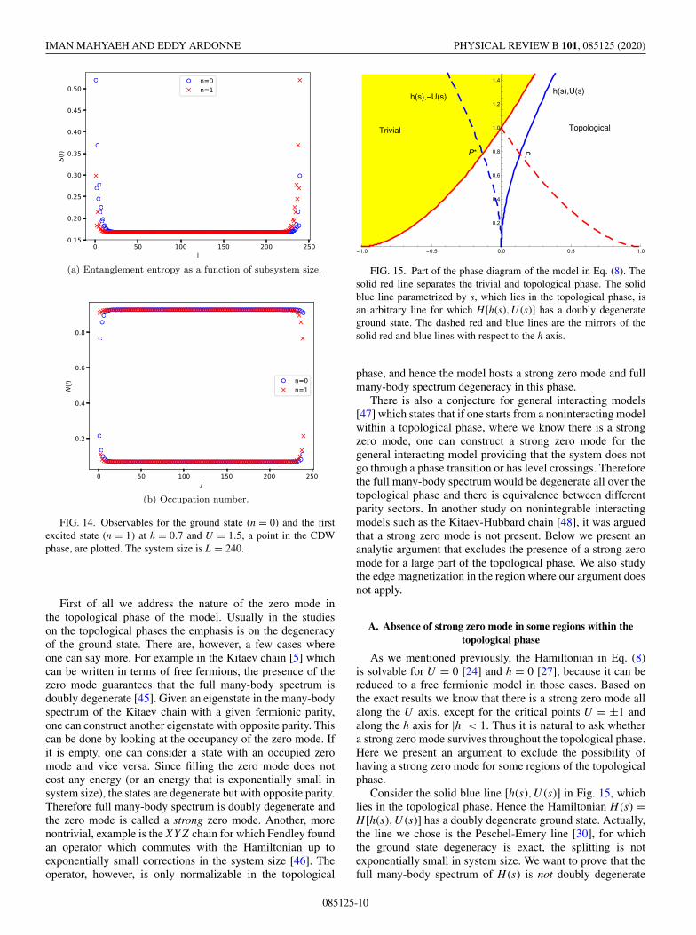
First of all we address the nature of the zero mode inthe topological phase of the model. Usually in the studieson the topological phases the emphasis is on the degeneracyof the ground state. There are, however, a few cases whereone can say more. For example in the Kitaev chain [5] whichcan be written in terms of free fermions, the presence of thezero mode guarantees that the full many-body spectrum isdoubly degenerate [45]. Given an eigenstate in the many-bodyspectrum of the Kitaev chain with a given fermionic parity,one can construct another eigenstate with opposite parity. Thiscan be done by looking at the occupancy of the zero mode. Ifit is empty, one can consider a state with an occupied zeromode and vice versa. Since filling the zero mode does notcost any energy (or an energy that is exponentially small insystem size), the states are degenerate but with opposite parity.Therefore full many-body spectrum is doubly degenerate andthe zero mode is called a strong zero mode. Another, morenontrivial, example is the XY Z chain for which Fendley foundan operator which commutes with the Hamiltonian up toexponentially small corrections in the system size [46]. Theoperator, however, is only normalizable in the topological

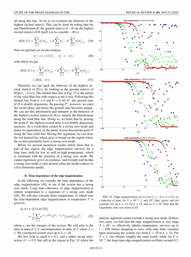
FIG. 15. Part of the phase diagram of the model in Eq. (8). Thesolid red line separates the trivial and topological phase. The solidblue line parametrized by s, which lies in the topological phase, isan arbitrary line for which H [h(s),U (s)] has a doubly degenerateground state. The dashed red and blue lines are the mirrors of thesolid red and blue lines with respect to the h axis.

phase, and hence the model hosts a strong zero mode and fullmany-body spectrum degeneracy in this phase.

There is also a conjecture for general interacting models[47] which states that if one starts from a noninteracting modelwithin a topological phase, where we know there is a strongzero mode, one can construct a strong zero mode for thegeneral interacting model providing that the system does notgo through a phase transition or has level crossings. Thereforethe full many-body spectrum would be degenerate all over thetopological phase and there is equivalence between differentparity sectors. In another study on nonintegrable interactingmodels such as the Kitaev-Hubbard chain [48], it was arguedthat a strong zero mode is not present. Below we present ananalytic argument that excludes the presence of a strong zeromode for a large part of the topological phase. We also studythe edge magnetization in the region where our argument doesnot apply.

A. Absence of strong zero mode in some regions within thetopological phase

As we mentioned previously, the Hamiltonian in Eq. (8)is solvable for U = 0 [24] and h = 0 [27], because it can bereduced to a free fermionic model in those cases. Based onthe exact results we know that there is a strong zero mode allalong the U axis, except for the critical points U = ±1 andalong the h axis for |h| < 1. Thus it is natural to ask whethera strong zero mode survives throughout the topological phase.Here we present an argument to exclude the possibility ofhaving a strong zero mode for some regions of the topologicalphase.

Consider the solid blue line [h(s),U (s)] in Fig. 15, whichlies in the topological phase. Hence the Hamiltonian H (s) =H[h(s),U (s)] has a doubly degenerate ground state. Actually,the line we chose is the Peschel-Emery line [30], for whichthe ground state degeneracy is exact, the splitting is notexponentially small in system size. We want to prove that thefull many-body spectrum of H (s) is not doubly degenerate

085125-10

STUDY OF THE PHASE DIAGRAM OF THE … PHYSICAL REVIEW B 101, 085125 (2020)

all along this line. To do so we examine the behavior of thehighest excited state(s). This can be done by noting that forany Hamiltonian H , the ground state(s) of −H are the highestexcited state(s) of H itself. Let us consider −H (s),

−H (h,U ) =L−1∑j=1

σ xj σ

xj+1 + h

L∑j=1

σ zj − U

L−1∑j=1

σ zj σ

zj+1. (29)

Now we perform an on-site rotation,

σ xj → (−1) jσ x

j , σ zj → −σ z

j , (30)

with which we get

−H (h,U ) = −L−1∑j=1

σ xj σ

xj+1 − h

L∑j=1

σ zj − U

L−1∑j=1

σ zj σ

zj+1

= H (h,−U ). (31)

Therefore we can track the behavior of the highest ex-cited state(s) of H (s), by looking at the ground state(s) ofH[h(s),−U (s)]. The dashed blue line in Fig. 15 is the mirrorof the solid blue line with respect to the h axis. Following thisdashed line from h = 0 and U = 0 till P∗, the ground stateof H is doubly degenerate. By passing P∗, however, we enterthe trivial phase and hence the ground state becomes unique.We can use this information and interpret as the behavior ofthe highest excited state(s) of H (s), namely the Hamiltonianalong the solid blue line. Doing so, we learn that by passingthe point P, the highest excited state is not doubly degenerateanymore. As a result there cannot be a strong zero mode andhence no equivalence of the parity sectors beyond the point Palong the blue solid line. Having this argument, we can drawthe red dashed line which gives a bound on the region wherethe system potentially hosts a strong zero mode.

Below we present numerical results which show that inpart of this region, the edge magnetization survives for along time, both for low as well as high temperature, whichis consistent with the presence of a strong zero mode. Wecannot rigorously prove its existence, and it might well be thata strong zero mode is only present when the model reduces toa free-fermionic model.

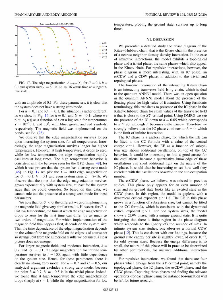
B. Time dependence of the edge magnetization

In the following we consider the time dependence of theedge magnetization [48], to see if the system has a strongzero mode. Long time coherence of edge magnetization atinfinite temperature is a signature of a strong zero mode[48]. We will also consider finite temperature, in which casethe time-dependent edge magnetization at temperature T isgiven by

AT (t ) = ⟨σ x

1 (t )σ x1 (0)

⟩

= 1

Z

∑j1, j2

e−ε j1 /(kT )ei(ε j1 −ε j2 )t∣∣〈 j2|σ x

1 | j1〉∣∣2

, (32)

where ε j are the energies of the system. We will refer to thetime in units of 1/J , and temperature in units of J , where J =1. We considered system sizes up to L = 16.

We first look at small h = 0.1, and a rather strong inter-action |U | = 0.5, but still in the region in Fig. 15 where the

FIG. 16. Edge magnetization |AT (t )| for U = −0.1, h = 0.1, asa function of time, for T = 10−3, 1, and 103, blue, green, and redsymbols, for (a) L = 12, (b) L = 14, and (c) L = 16. Note that thelogarithmic time axis starts at 103.

analytic argument cannot exclude a strong zero mode. In thesetwo cases, we find that the edge magnetization at very largeT = 103, so effectively infinite temperature, survives up tot ∼ 100, before dropping to zero, with only little variationupon increasing the system size from L = 10 to L = 14. ForT = 1, one obtains roughly the same result, while for T =10−3, the long-time edge magnetization oscillates around 0.7,

085125-11

IMAN MAHYAEH AND EDDY ARDONNE PHYSICAL REVIEW B 101, 085125 (2020)

FIG. 17. The edge magnetization |AT =1000(t )| for U = 0.1, h =0.1 and system sizes L = 8, 10, 12, 14, 16 versus time on a logarith-mic scale.

with an amplitude of 0.1. For these parameters, it is clear thatthe system does not have a strong zero mode.

For h = 0.1 and |U | = 0.1, the situation is rather different,as we show in Fig. 16 for h = 0.1 and U = −0.1, where weplot |AT (t )| as a function of t on a log scale for temperaturesT = 10−3, 1, and 103, with blue, green, and red symbols,respectively. The magnetic field was implemented on thebonds, see Eq. (23).

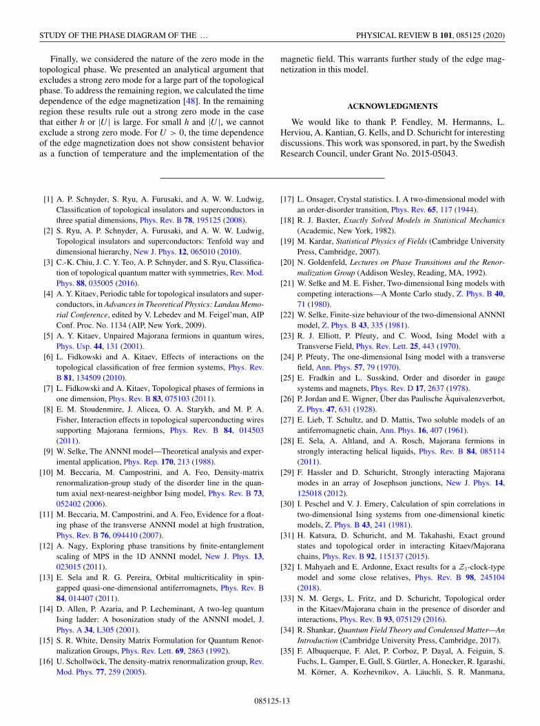
We observe that the edge magnetization survives longerupon increasing the system size, for all temperatures. Inter-estingly, the edge magnetization survives longer for highertemperatures. However, at high temperature, it drops to zero,while for low temperature, the edge magnetization rapidlyoscillates at long times. The high temperature behavior isconsistent with the behavior seen for the XY Z chain [48], forwhich it was proven that the system has a strong zero mode[46]. In Fig. 17 we plot the T = 1000 edge magnetizationfor U = 0.1, h = 0.1 and even system sizes L = 8–16. Weobserve that the time that the edge magnetization survivesgrows exponentially with system size, at least for the systemsizes that we could consider. So based on this data, wecannot rule out the presence of a strong zero mode for theseparameters.

We note that for U < 0, the different ways of implementingthe magnetic field give very similar results. However, for U >

0 at low temperature, the time at which the edge magnetizationdrops to zero for the first time can differ by as much astwo orders of magnitude. For which implementation of themagnetic field this happens first, depends on the system size.That the time dependence of the edge magnetization dependson the value of the magnetic field on the edges is of course notso strange, but from the numerical results we obtained, a clearpicture does not emerge.

For larger magnetic fields and moderate interaction, h =0.7, and |U | = 0.1, the edge magnetization for infinite tem-perature survives to t ∼ 100, again with little dependenceon the system size. Hence, for these parameters, there isclearly no strong zero mode. For h = 0.7 and U = 0.5, ouranalytical argument excludes a strong zero mode, becausethe point h = 0.7, U = −0.5 is in the trivial phase. Indeed,we found that at high temperature the edge magnetizationdrops sharply at t ∼ 1, while the edge magnetization for low

temperature, probing the ground state, survives up to longtimes.

VI. DISCUSSION

We presented a detailed study the phase diagram of theKitaev-Hubbard chain, that is the Kitaev chain in the presenceof a nearest-neighbor density-density interaction. In the caseof attractive interactions, the model exhibits a topologicalphase and a trivial phase, the same phases which also appearin the Kitaev chain. For repulsive interactions, however, thephase diagram is more interesting, with an IC phase, anesCDW and a CDW phase, in addition to the trivial andtopological phases.

The bosonic incarnation of the interacting Kitaev chainis an interacting transverse field Ising chain, which is dualto the quantum ANNNI model. There was an open questionin the quantum ANNNI model about the presence of thefloating phase for high value of frustration. Using fermionicterminology, this translates to presence of the IC phase in theKitaev-Hubbard chain for small values of the transverse fieldh that is close to the XY critical point. Using DMRG we seethe presence of the IC down to h = 0.05 which correspondsto κ � 20, although it becomes quite narrow. Therefore westrongly believe that the IC phase continues to h = 0, whichis the limit of infinite frustration.

The IC phase is a gapless phase, for which the EE canbe fitted to the CC formula with a value of the centralcharge c � 1. However, the EE as a function of subsys-tem size shows additional oscillations, on top of the CCbehavior. It would be interesting to find a good ansatz forthe oscillations, because a quantitative knowledge of theseoscillations can shed additional light on the nature of theIC phase. It would also be interesting to see how well theycorrelate with the oscillations observed in the site occupationnumber.

The esCDW phase, we believe, was missed in previousstudies. This phase only appears for an even number ofsites and its ground state looks like an excited state in theCDW phase. In this region, the model is gapless, with adynamical critical exponent z � 1.8. The EE in this phasegrows as a function of subsystem size, but cannot be fittedto the CC formula, which is consistent with the dynamicalcritical exponent z > 1. For odd system sizes, the modelshows a CDW phase, with a unique ground state. It is quiteintriguing that there is finite region in the phase diagramwhich responds to the (parity of) the number of sites. Ininfinite system size studies, one observes a normal CDWphase [12]. This is consistent with our findings, because theground state energy per site is slightly lower, of order 10−3,for odd system sizes. Because the energy difference is sosmall, the nature of this phase will in practice be determinedby other perturbations, for instance additional interactionterms.

For repulsive interactions, we found that there are fourphases which emerge from the XY critical point, namely thetopological phase, the IC phase, the esCDW phase, and theCDW phase. Capturing these phases and finding the relevantoperator(s) for each phase using for instance bosonization willbe left for future research.

085125-12

STUDY OF THE PHASE DIAGRAM OF THE … PHYSICAL REVIEW B 101, 085125 (2020)

Finally, we considered the nature of the zero mode in thetopological phase. We presented an analytical argument thatexcludes a strong zero mode for a large part of the topologicalphase. To address the remaining region, we calculated the timedependence of the edge magnetization [48]. In the remainingregion these results rule out a strong zero mode in the casethat either h or |U | is large. For small h and |U |, we cannotexclude a strong zero mode. For U > 0, the time dependenceof the edge magnetization does not show consistent behavioras a function of temperature and the implementation of the

magnetic field. This warrants further study of the edge mag-netization in this model.

ACKNOWLEDGMENTS

We would like to thank P. Fendley, M. Hermanns, L.Herviou, A. Kantian, G. Kells, and D. Schuricht for interestingdiscussions. This work was sponsored, in part, by the SwedishResearch Council, under Grant No. 2015-05043.

[1] A. P. Schnyder, S. Ryu, A. Furusaki, and A. W. W. Ludwig,Classification of topological insulators and superconductors inthree spatial dimensions, Phys. Rev. B 78, 195125 (2008).

[2] S. Ryu, A. P. Schnyder, A. Furusaki, and A. W. W. Ludwig,Topological insulators and superconductors: Tenfold way anddimensional hierarchy, New J. Phys. 12, 065010 (2010).

[3] C.-K. Chiu, J. C. Y. Teo, A. P. Schnyder, and S. Ryu, Classifica-tion of topological quantum matter with symmetries, Rev. Mod.Phys. 88, 035005 (2016).

[4] A. Y. Kitaev, Periodic table for topological insulators and super-conductors, in Advances in Theoretical Physics: Landau Memo-rial Conference, edited by V. Lebedev and M. Feigel’man, AIPConf. Proc. No. 1134 (AIP, New York, 2009).

[5] A. Y. Kitaev, Unpaired Majorana fermions in quantum wires,Phys. Usp. 44, 131 (2001).

[6] L. Fidkowski and A. Kitaev, Effects of interactions on thetopological classification of free fermion systems, Phys. Rev.B 81, 134509 (2010).

[7] L. Fidkowski and A. Kitaev, Topological phases of fermions inone dimension, Phys. Rev. B 83, 075103 (2011).

[8] E. M. Stoudenmire, J. Alicea, O. A. Starykh, and M. P. A.Fisher, Interaction effects in topological superconducting wiressupporting Majorana fermions, Phys. Rev. B 84, 014503(2011).

[9] W. Selke, The ANNNI model—Theoretical analysis and exper-imental application, Phys. Rep. 170, 213 (1988).

[10] M. Beccaria, M. Campostrini, and A. Feo, Density-matrixrenormalization-group study of the disorder line in the quan-tum axial next-nearest-neighbor Ising model, Phys. Rev. B 73,052402 (2006).

[11] M. Beccaria, M. Campostrini, and A. Feo, Evidence for a float-ing phase of the transverse ANNNI model at high frustration,Phys. Rev. B 76, 094410 (2007).

[12] A. Nagy, Exploring phase transitions by finite-entanglementscaling of MPS in the 1D ANNNI model, New J. Phys. 13,023015 (2011).

[13] E. Sela and R. G. Pereira, Orbital multicriticality in spin-gapped quasi-one-dimensional antiferromagnets, Phys. Rev. B84, 014407 (2011).

[14] D. Allen, P. Azaria, and P. Lecheminant, A two-leg quantumIsing ladder: A bosonization study of the ANNNI model, J.Phys. A 34, L305 (2001).

[15] S. R. White, Density Matrix Formulation for Quantum Renor-malization Groups, Phys. Rev. Lett. 69, 2863 (1992).

[16] U. Schollwöck, The density-matrix renormalization group, Rev.Mod. Phys. 77, 259 (2005).

[17] L. Onsager, Crystal statistics. I. A two-dimensional model withan order-disorder transition, Phys. Rev. 65, 117 (1944).

[18] R. J. Baxter, Exactly Solved Models in Statistical Mechanics(Academic, New York, 1982).

[19] M. Kardar, Statistical Physics of Fields (Cambridge UniversityPress, Cambridge, 2007).

[20] N. Goldenfeld, Lectures on Phase Transitions and the Renor-malization Group (Addison Wesley, Reading, MA, 1992).

[21] W. Selke and M. E. Fisher, Two-dimensional Ising models withcompeting interactions—A Monte Carlo study, Z. Phys. B 40,71 (1980).

[22] W. Selke, Finite-size behaviour of the two-dimensional ANNNImodel, Z. Phys. B 43, 335 (1981).

[23] R. J. Elliott, P. Pfeuty, and C. Wood, Ising Model with aTransverse Field, Phys. Rev. Lett. 25, 443 (1970).

[24] P. Pfeuty, The one-dimensional Ising model with a transversefield, Ann. Phys. 57, 79 (1970).

[25] E. Fradkin and L. Susskind, Order and disorder in gaugesystems and magnets, Phys. Rev. D 17, 2637 (1978).

[26] P. Jordan and E. Wigner, Über das Paulische Äquivalenzverbot,Z. Phys. 47, 631 (1928).

[27] E. Lieb, T. Schultz, and D. Mattis, Two soluble models of anantiferromagnetic chain, Ann. Phys. 16, 407 (1961).

[28] E. Sela, A. Altland, and A. Rosch, Majorana fermions instrongly interacting helical liquids, Phys. Rev. B 84, 085114(2011).

[29] F. Hassler and D. Schuricht, Strongly interacting Majoranamodes in an array of Josephson junctions, New J. Phys. 14,125018 (2012).

[30] I. Peschel and V. J. Emery, Calculation of spin correlations intwo-dimensional Ising systems from one-dimensional kineticmodels, Z. Phys. B 43, 241 (1981).

[31] H. Katsura, D. Schuricht, and M. Takahashi, Exact groundstates and topological order in interacting Kitaev/Majoranachains, Phys. Rev. B 92, 115137 (2015).

[32] I. Mahyaeh and E. Ardonne, Exact results for a Z3-clock-typemodel and some close relatives, Phys. Rev. B 98, 245104(2018).

[33] N. M. Gergs, L. Fritz, and D. Schuricht, Topological orderin the Kitaev/Majorana chain in the presence of disorder andinteractions, Phys. Rev. B 93, 075129 (2016).

[34] R. Shankar, Quantum Field Theory and Condensed Matter—AnIntroduction (Cambridge University Press, Cambridge, 2017).

[35] F. Albuquerque, F. Alet, P. Corboz, P. Dayal, A. Feiguin, S.Fuchs, L. Gamper, E. Gull, S. Gürtler, A. Honecker, R. Igarashi,M. Körner, A. Kozhevnikov, A. Läuchli, S. R. Manmana,

085125-13

IMAN MAHYAEH AND EDDY ARDONNE PHYSICAL REVIEW B 101, 085125 (2020)

M. Matsumoto, I. P. McCulloch, F. Michel, R. M. Noack, G.Pawlowski, L. Pollet, T. Pruschke, U. Schollwöck, S. Todo, S.Trebst, M. Troyer, P. Werner, S. Wessel, and for the ALPS col-laboration, The ALPS project release 1.3: Open-source softwarefor strongly correlated systems, J. Magn. Magn. Mater. 310,1187 (2007).

[36] B. Bauer, L. D. Carr, H. G. Evertz, A. Feiguin, J. Freire, S.Fuchs, L. Gamper, J. Gukelberger, E. Gull, S. Güertler, A.Hehn, R. Igarashi, S. V. Isakov, D. Koop, P. N. Ma, P. Mates,H. Matsuo, O. Parcollet, G. Pawlowski, J. D. Picon, L. Pollet,E. Santos, V. W. Scarola, U. Schollwöck, C. Silva, B. Surer,S. Todo, S. Trebst, M. Troyer, M. L. Wall, P. Werner, and S.Wessel, The ALPS project release 2.0: open source software forstrongly correlated systems, J. Stat. Mech. (2011) P05001.

[37] M. Dolfi, B. Bauer, S. Keller, A. Kosenkov, T. Ewart, A.Kantian, T. Giamarchi, and M. Troyer, Matrix product stateapplications for the ALPS project, Comput. Phys. Commun.185, 3430 (2014).

[38] M. E. Fisher and M. N. Barber, Scaling Theory for Finite-SizeEffects in the Critical Region, Phys. Rev. Lett. 28, 1516 (1972).

[39] S. Sachdev, Quantum Phase Transitions (Cambridge UniversityPress, Cambridge, 2011).

[40] P. Di Francesco, P. Mathieu, and D. Sénéchal, Conformal FieldTheory (Springer, New York, 1999).

[41] P. Calabrese and J. Cardy, Entanglement entropy and quantumfield theory, J. Stat. Mech. (2004) P06002.

[42] P. Calabrese and J. Cardy, Entanglement entropy and conformalfield theory, J. Phys. A: Math. Theor. 42, 504005 (2009).

[43] C. Holzhey, F. Larsen, and F. Wilczek, Geometric and renor-malized entropy in conformal field theory, Nucl. Phys. B 424,443 (1994).

[44] Y. Zhuang, H. J. Changlani, N. M. Tubman, and T. L. Hughes,Phase diagram of the Z3 parafermionic chain with chiral inter-actions, Phys. Rev. B 92, 035154 (2015).

[45] P. Fendley, Parafermionic edge zero modes in Zn-invariant spinchains, J. Stat. Mech. (2012) P11020.

[46] P. Fendley, Strong zero modes and eigenstate phase transitionsin the XYZ/interacting Majorana chain, J. Phys. A: Math.Theor. 49, 30LT01 (2016).

[47] G. Kells, Many-body Majorana operators and the equiv-alence of parity sectors, Phys. Rev. B 92, 081401(R)(2015).

[48] J. Kemp, N. Y. Yao, C. R. Laumann, and P. Fendley, Longcoherence times for edge spins, J. Stat. Mech. (2017) 063105.

085125-14