Physica A xx (xxxx) xxx–xxx

Contents lists available at ScienceDirect

Physica A

journal homepage: www.elsevier.com/locate/physa

Study of the influence of the phylogenetic distance on theinteraction network of mutualistic ecosystems

Q1 Roberto P.J. Perazzo a, Laura Hernández b,∗, Horacio Ceva c, Enrique Burgos c,d,José Ignacio Alvarez-Hamelin a

a Departamento de Investigación y Desarrollo, Instituto Tecnológico de Buenos Aires, Avenida E. Madero 399, Buenos Aires, Argentinab Laboratoire de Physique Théorique et Modélisation, UMR CNRS, Université de Cergy-Pontoise, 2 Avenue Adolphe Chauvin, 95302,Cergy-Pontoise Cedex, Francec Departamento de Física, Comisión Nacional de Energía Atómica, Avenida del Libertador, 8250, 1429 Buenos Aires, Argentinad Consejo Nacional de Investigaciones Científicas y Técnicas, Avenida Rivadavia 1917, C1033AAJ, Buenos Aires, Argentina

h i g h l i g h t s

• We study the influence of phylogenetic distance on mutualistic ecosystems’ networks.• Instead of a statistical study, we reformulated it as an optimization problem.• We generalize the self-organizing network model (SNM) to handle phylogenetic data.• Reducing the distance among the counterparts of each species destroys nestedness.

a r t i c l e i n f o

Article history:Received 27 April 2013Received in revised form 19 August 2013Available online xxxx

a b s t r a c t

We investigate how the phylogenetic relationship between the species of each interactingguild in a mutualistic ecosystem influences its network of contacts. We develop adynamical self organizedmodel that reallocates contacts betweenmutualists, according toa contact preference rule (CPR) that takes into account phylogenetic distances.We concludethat a CPR that promotes phylogenetic proximity among the counterparts of the species ofeach guild leads to highly unrealistic contact patterns. We find that nestedness can insteadbe attributed to a general rule by which species tend to behave as generalists holdingcontacts with counterparts that already have a large number of contacts.

© 2013 Elsevier B.V. All rights reserved.Q2

1. Introduction 1

Mutualistic ecosystems usually involve species of animals and plants that interact to fulfill essential biological functions 2

such as feeding or reproduction. Typical examples are pollination networks, where insects feeding from the nectar of 3

flowers contribute to the pollination process and seed dispersal networks, where animals (usually birds) feed from the 4

fruits while dispersing the seeds contained in them. A large amount of research has been devoted to studying mutualism 5

[1,2]. In traditional studies, the interaction of all active plant and animal species is recorded within a restricted geographical 6

extension [3,4]. Collecting these data is a difficult work and several observed ecosystems are not large enough so as to obtain 7

reasonable statistical results. Interestingly, some large ecosystems have been recorded like for example [5–7]. 8

∗ Corresponding author. Tel.: +33 134257521; fax: +33 134257500.E-mail addresses: rperazzo@itba.edu.ar (R.P.J. Perazzo), laura.hernandez@u-cergy.fr, laura.hernandez1@sfr.fr (L. Hernández), ceva@cnea.gov.ar

(H. Ceva), burgos@cnea.gov.ar (E. Burgos), ihameli@cnet.fi.uba.ar (J.I. Alvarez-Hamelin).

0378-4371/$ – see front matter© 2013 Elsevier B.V. All rights reserved.http://dx.doi.org/10.1016/j.physa.2013.08.052

2 R.P.J. Perazzo et al. / Physica A xx (xxxx) xxx–xxx

The interaction among the mutualists may be described in terms of a complex network which is said to be bipartite as1

there are two different kind of vertices, those representing plant species and those representing animal species, while the2

considered interactions only happen between vertices of different kinds.3

The corresponding adjacency matrices of natural mutualistic ecosystems strongly indicate that they are not a random4

collection of interacting species, but that they display instead a high degree of internal organization. A pervading feature that5

is generally found is that such adjacency matrices have a nested pattern of interactions, in which both generalists (species6

holding many interactions) and specialists (holding few interactions) tend to interact with generalists whereas specialist-7

to-specialist interactions are infrequent [8]. In other words, if species are ordered by decreasing number of contacts, then8

the contacts of a given species constitute a subset of the contacts of the preceding species in the list [9].9

This nested structure has been attributed to a number of different causes and the controversy about the ultimate reasons10

making this pattern so frequently observed is still open. It is fairly obvious that a detailed explanation of the interaction11

behavior of individual species can be of little help to understand such a generalized pattern found in ecological systems of12

very different sizes and types, and involving plants of different nature and animals that range from insects to birds.13

Nestedness has been shown to offer some advantage for the robustness of thewhole system; thus suggesting that systems14

that are currently observed are those that have survived less disturbed thanks to its nested structure [8,10].15

Interestingly, the same nested structure has been recently found in a completely different context: industrial structure16

of the countries and the import–export world trade network. In these cases the two different kinds of nodes represent the17

products and the countries that produce or buy them. It has been shown that the techniques used to measure the degree of18

order of mutualistic ecosystems seem to be adapted to a description of these economical systems and that they are more19

precise than the magnitudes habitually used to address these problems such as, for instance, the global amount of products20

bought/sold by each country [11–14].21

Different hypotheses aiming to explain the origin of this widespread pattern of interactions in mutualist ecosystems22

have been proposed. In Ref. [15] nestedness has been attributed to phenotypic affinity between species of different guilds23

while in Refs. [16,17] an extensive analysis is performed, concluding that phylogenetic proximity could explain the nested24

organization of contacts of some cases of mutualistic systems. Ref. [18] considers the contrary, that the modest percentage25

of correlations between phylogenetic relatedness and ecological similarity found in Ref. [16] indicates that phylogenetic26

relationships do not have a marked effect.27

Most of the works that study the possible mechanisms that lead to this nested pattern search for a positive statistical28

correlation between the nested pattern of contacts and its supposed cause. However, the sole fact that in a part of the29

empirical observations two elements appear to be statistically correlated should not be taken tomean that one is the cause of30

the other. Such a correlationmay rather indicate instead, that both elements are not incompatible, i.e., they do not mutually31

exclude each other or they stem from a third, common cause.32

One example of this analysis is given by the strong positive correlation found between the species’ abundance and hence33

the frequency of interactions, with the pattern of contacts of some species [19]. It has been suggested that locally abundant34

species are prone to accumulate interactions and conversely rare species are prone to lose them [20], as also suggested by35

neutral theories [21].36

We propose an alternative way to identify the important features that may lead to nestedness, by studying the states37

reached by a system that follows a dynamical process based on some assumed interaction mechanism between the38

mutualists, thus comforting or falsifying hypotheses concerning such interaction mechanisms between the species. This39

complementary approach is based on the Self Organizing Network Model (SNM) that we have proposed and developed in40

Refs. [22,23] and that we will briefly recall in Section 2.1.41

In the present paper we generalize the SNM in order to integrate external data that is not contained in the evolving42

network but has to be taken from the phylogenetic trees of the interacting mutualists. Mathematically, phylogenetic43

proximity is accounted for through a matrix of distances separating any two species of each guild. The distance matrix44

is directly obtained from the topology of the phylogenetic tree.45

We complete our studywith the comparison of the statistical properties of observed networkswith those of two extreme46

idealized benchmarks.47

2. Description of the numerical study48

2.1. The SNM algorithm49

Mutualistic systems can be analyzed as bipartite graphs [24]. The interaction pattern is usually coded into a (rectangular)50

adjacency matrix in which rows and columns are labeled respectively by the plant and animal species. Its elements51

Kp,a ∈ {0, 1} represent respectively the absence or presence of an interaction (contact) between the plant species p and52

the animal species a. The number of contacts of each species is the degree of the corresponding node in the bipartite graph,53

GA,(P)

a,(p) , for animals (plants).54

Several reasons have been given to explain the pattern of interactions between the two guilds of a mutualistic network.55

They have been usually based on positive statistical significance of correlations. One alternative way to elucidate a possible56

causal link between some hypothetical interaction mechanisms between mutualistic species and the pattern of contacts, is57

to use a dynamical model.58

R.P.J. Perazzo et al. / Physica A xx (xxxx) xxx–xxx 3

The basic idea behind this strategy is to verify the consistency of the empirically observed contact pattern, and some 1

hypothetical interaction rule that may favor or hamper the contact between mutualistic species. Such interaction can, in 2

principle, be based on phenotypic complementarity, phylogenetic affinity, degree, or any other possibility. We call the 3

interaction mechanism the contact preference rule (CPR) in the sense that it is assumed that species verifying this rule tend 4

to hold contacts among each other. 5

The dynamics of the SNM is artificial and should not be interpreted as representing the complex evolutionary processes 6

that have led to the species themselves as observed today and to their interactions. Instead, from a purely theoretical point of 7

view, this setup is equivalent to considering that the observed pattern of interactions corresponds to an optimal assignment 8

of the contacts between both guilds, with two constraints. The first constraint is the fulfillment of an assumed CPR, and the 9

second is the given (constant) total number of contacts between the twomutualistic guilds. This numbermight be considered 10

as an indicator of the energy invested by all the species of the ecological system in their exchange of nourishment. In other 11

words onemay attempt to describe the observed pattern of contacts as the result of a (combinatorial) optimization problem 12

by which contacts in the adjacency matrix are placed in such a way so as to reach an extreme of an utility function that 13

corresponds to an optimal fulfillment of some prevailing CPR. 14

Comparing with the real system, the pattern that emerges when running the SNM with the chosen CPR, starting from 15

an initial random adjacency matrix, one can easily rule out the wrong hypothesis when the reached stationary states differ 16

from the real system considered. This can also be done by analyzing the stability of real adjacency matrices evolved with 17

the studied CPR. 18

On the other hand an emerging pattern that is consistent with the organization of real systems suggests that the studied 19

CPR may be considered as playing an important role in the observed organization of the ecosystem. 20

In the SNM discussed in Refs. [8,22] the topology of that network emerges as the result of a self-organization process 21

where links are redefined gradually, alternating plants and animals. For instance, a plant is first chosen at random and one 22

of its contacts is redefined by spotting a mutualistic counterpart that has already more contacts that the original one (called 23

SNM-I in the previously cited references). Next an animal is chosen and the same procedure is accomplished. The iteration 24

of these steps provides a simple heuristic, leading to a good approximation of the optimal assignment of contactsmentioned 25

above. 26

Unlike in the preferential attachment algorithm [25], in the SNM the topology of a non-growing network with a fixed 27

number of nodes is progressively reshaped: at each iteration a connection between two nodes of different kinds is rewired 28

to favor a contact with the node having the highest degree. It is worthwhile noting that in this sense, the CPR of the SNM 29

is local: it does not take into account the whole probability distribution, but only the degrees of the two randomly chosen 30

species. 31

In the above references we show that such a CPR always leads to nested networks with degree distributions that closely 32

resemble the ones reported from the observation of real mutualistic systems. 33

The SNMhas to bemodified to take into consideration the phylogenetic structure of both guilds. Therefore, it is necessary 34

to have a simple quantitative measure of the phylogenetic structure. We now describe how this is made. 35

2.2. The phylogenetic-SNM 36

To study the influence of phylogenetic proximity on the pattern formation of the adjacency matrix, one has to modify 37

the SNM by properly defining a CPR based on some measure of the phylogenetic distance between any two species of the 38

same guild. 39

The classification of species according to their similarities has been a major endeavor since the origins of biology as 40

a natural science. This classification may be summarized in a symmetric N × N distance matrix with vanishing diagonal 41

elements providing ameasure of similarities and differences between any pair of species. Due to the central role of evolution, 42

these classifications are depicted by phylogenetic trees that are determined using several sources of information. 43

Comparative studies of phenotypic traits are also widely used. The resemblance of species is measured through a 44

phylogenetic signal that is quantitatively estimated through statistical analyses [26,27] of the distribution of the values 45

of different traits. These studies may also be supplemented whenever possible with fossil records. 46

While the tips of the tree correspond to presently observed species, the remaining nodes are associated to their presumed 47

ancestors. A hierarchical organization of all living species is therefore provided and those that closely resemble each other 48

are neighboring tips of the tree. 49

The phylogenetic classification of a group of species gathers them in taxa within taxa of an ever increasing generality. 50

Based on the topology of the tree it is possible to define a distance that provides a quantitative estimation of resemblances 51

and differences between them. In the appendix we describe the simple procedure to extract a distance matrix directly from 52

the topology of the phylogenetic tree. 53

A distance matrix d(k, k′) constructed in this way is not only fully consistent from the start with the results of statistical 54

analyses but also fully agrees with what can be expected from an intuitive picture: small values of d(k, k′) remain associated 55

to species that share the same branching sequence and a common evolutionary history while large values correspond to 56

species that have followed a different evolutionary process because they have been separated at earlier stages. With these 57

conventions the closest possible distance between any two species is 1 and, if all species are at a distance 1 they belong to 58

a star phylogeny. 59

4 R.P.J. Perazzo et al. / Physica A xx (xxxx) xxx–xxx

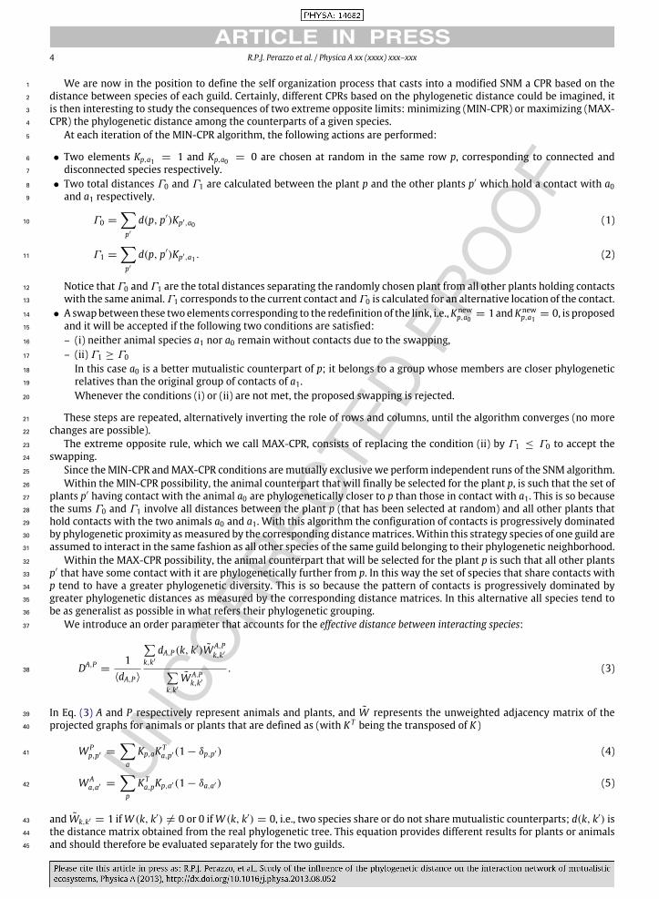
We are now in the position to define the self organization process that casts into a modified SNM a CPR based on the1

distance between species of each guild. Certainly, different CPRs based on the phylogenetic distance could be imagined, it2

is then interesting to study the consequences of two extreme opposite limits: minimizing (MIN-CPR) or maximizing (MAX-3

CPR) the phylogenetic distance among the counterparts of a given species.4

At each iteration of the MIN-CPR algorithm, the following actions are performed:5

• Two elements Kp,a1 = 1 and Kp,a0 = 0 are chosen at random in the same row p, corresponding to connected and6

disconnected species respectively.7

• Two total distances Γ0 and Γ1 are calculated between the plant p and the other plants p′ which hold a contact with a08

and a1 respectively.9

Γ0 =

p′

d(p, p′)Kp′,a0 (1)10

Γ1 =

p′

d(p, p′)Kp′,a1 . (2)11

Notice that Γ0 and Γ1 are the total distances separating the randomly chosen plant from all other plants holding contacts12

with the same animal.Γ1 corresponds to the current contact andΓ0 is calculated for an alternative location of the contact.13

• A swapbetween these two elements corresponding to the redefinition of the link, i.e.,Knewp,a0 = 1 andKnew

p,a1 = 0, is proposed14

and it will be accepted if the following two conditions are satisfied:15

– (i) neither animal species a1 nor a0 remain without contacts due to the swapping,16

– (ii) Γ1 ≥ Γ017

In this case a0 is a better mutualistic counterpart of p; it belongs to a group whose members are closer phylogenetic18

relatives than the original group of contacts of a1.19

Whenever the conditions (i) or (ii) are not met, the proposed swapping is rejected.20

These steps are repeated, alternatively inverting the role of rows and columns, until the algorithm converges (no more21

changes are possible).22

The extreme opposite rule, which we call MAX-CPR, consists of replacing the condition (ii) by Γ1 ≤ Γ0 to accept the23

swapping.24

Since theMIN-CPR andMAX-CPR conditions aremutually exclusive we perform independent runs of the SNM algorithm.25

Within the MIN-CPR possibility, the animal counterpart that will finally be selected for the plant p, is such that the set of26

plants p′ having contact with the animal a0 are phylogenetically closer to p than those in contact with a1. This is so because27

the sums Γ0 and Γ1 involve all distances between the plant p (that has been selected at random) and all other plants that28

hold contacts with the two animals a0 and a1. With this algorithm the configuration of contacts is progressively dominated29

by phylogenetic proximity asmeasured by the corresponding distancematrices.Within this strategy species of one guild are30

assumed to interact in the same fashion as all other species of the same guild belonging to their phylogenetic neighborhood.31

Within the MAX-CPR possibility, the animal counterpart that will be selected for the plant p is such that all other plants32

p′ that have some contact with it are phylogenetically further from p. In this way the set of species that share contacts with33

p tend to have a greater phylogenetic diversity. This is so because the pattern of contacts is progressively dominated by34

greater phylogenetic distances as measured by the corresponding distance matrices. In this alternative all species tend to35

be as generalist as possible in what refers their phylogenetic grouping.36

We introduce an order parameter that accounts for the effective distance between interacting species:37

DA,P=

1⟨dA,P⟩

k,k′

dA,P(k, k′)W A,Pk,k′

k,k′W A.P

k,k′. (3)38

In Eq. (3) A and P respectively represent animals and plants, and W represents the unweighted adjacency matrix of the39

projected graphs for animals or plants that are defined as (with K T being the transposed of K )40

W Pp,p′ =

a

Kp,aK Ta,p′(1 − δp,p′) (4)41

W Aa,a′ =

p

K Ta,pKp,a′(1 − δa,a′) (5)42

and Wk,k′ = 1 ifW (k, k′) = 0 or 0 ifW (k, k′) = 0, i.e., two species share or do not share mutualistic counterparts; d(k, k′) is43

the distance matrix obtained from the real phylogenetic tree. This equation provides different results for plants or animals44

and should therefore be evaluated separately for the two guilds.45

R.P.J. Perazzo et al. / Physica A xx (xxxx) xxx–xxx 5

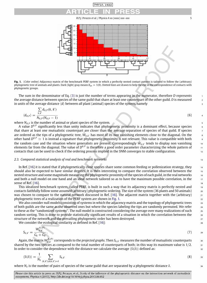
Fig. 1. (Color online) Adjacency matrix of the benchmark PERF system in which a perfectly nested contact pattern is tailored to follow the (arbitrary)phylogenetic tree of animals and plants. Dark (light) gray means Kpa = 1(0). Dotted lines are drawn to help the eye in the correspondence of contacts withphylogenetic groups.

The sum in the denominator of Eq. (3) is just the number of terms appearing in the numerator, therefore D represents 1

the average distance between species of the same guild that share at least one counterpart of the other guild. D is measured 2

in units of the average distance ⟨d⟩ between all plant (animal) species of the system, namely 3

⟨dA,P⟩ =

k,k′

dA,P(k, k′)

NA,P(NA,P − 1)(6) 4

where NA,P is the number of animal or plant species of the system. 5

A value DA,P significantly less than unity indicates that phylogenetic proximity is a dominant effect, because species 6

that share at least one mutualistic counterpart are closer than the average separation of species of that guild. If species 7

are ordered as the tips of a phylogenetic tree, Wk,k′ has most of its non vanishing elements close to the diagonal. On the 8

other hand DA,P≃ 1 is instead a signature that phylogenetic proximity is not relevant. This value is compatible with both 9

the random case and the situation where generalists are present. Correspondingly Wk,k′ tends to display non vanishing 10

elements far from the diagonal. The value of DA,P is therefore a good order parameter characterizing the whole pattern of 11

contacts that can be used to check if the ordering process implied in the SNM converges to stable configuration. 12

2.3. Compared statistical analysis of real and benchmark networks 13

In Ref. [16] it is stated that if phylogenetically close species share some common feeding or pollenization strategy, they 14

should also be expected to have similar degrees. It is then interesting to compare the correlation observed between the 15

nested structure and somemagnitudemeasuring thephylogenetic proximity of the species of each guild, in the real networks 16

and both a null model on one hand and an ideal network tailored so as to have the maximum possible correlation, in the 17

sense of Ref. [16]. 18

This idealized benchmark system, called PERF, is built in such a way that its adjacency matrix is perfectly nested and 19

contacts faithfully follow some assumed (arbitrary) phylogenetic ordering. The size of the system (36 plants and 50 animals) 20

was chosen to compare to the natural network discussed in Ref. [16]. The adjacent matrix together with the (arbitrary) 21

phylogenetic trees of a realization of the PERF system are shown in Fig. 1. 22

We also consider null models consisting of systems inwhich the adjacencymatrix and the topology of phylogenetic trees 23

of both guilds are the same as the observed ones but where the species labeling the tips are randomly permuted. We refer 24

to these as the ‘‘randomized systems’’. The null model is constructed considering the average over many realizations of such 25

random sorting. This is done to provide statistically significant results of a situation in which the correlation between the 26

structure of the network and the prevailing phylogenetic order has been destroyed. 27

We consider the ecological similarity as defined in Ref. [16]: 28

Sk,k′ =W A,(P)

k,k′

Gk + Gk′. (7) 29

Again, thematrixW A,(P)

k,k′ corresponds to the projected graphs. Then Sk,k′ measures the number of mutualistic counterparts 30

shared by the two species as compared to the total number of counterparts of both; in this way its maximum value is 1/2. 31

In order to consider the dependence with the distance we calculate the average ⟨S(δ)⟩ defined as: 32

⟨S(δ)⟩ =1Nδ

(k,k′)|d(k,k′)=δ

Sk,k′ (8) 33

where Nδ is the number of pairs of species of the same guild that are separated by a phylogenetic distance δ. 34

6 R.P.J. Perazzo et al. / Physica A xx (xxxx) xxx–xxx

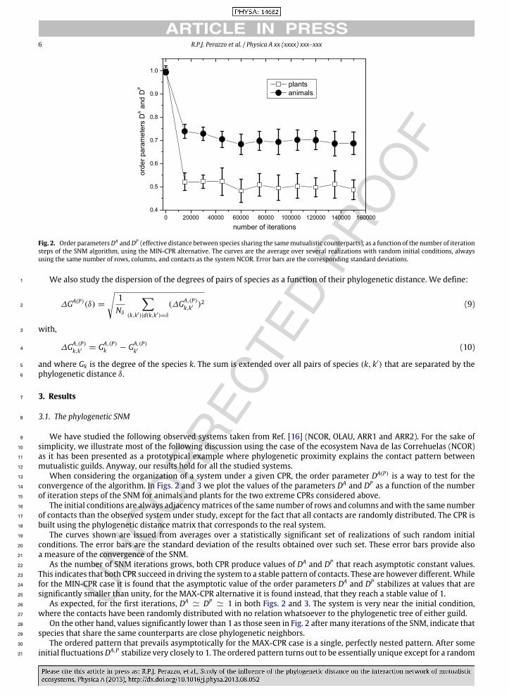
Fig. 2. Order parametersDA andDP (effective distance between species sharing the samemutualistic counterparts), as a function of the number of iterationsteps of the SNM algorithm, using the MIN-CPR alternative. The curves are the average over several realizations with random initial conditions, alwaysusing the same number of rows, columns, and contacts as the system NCOR. Error bars are the corresponding standard deviations.

We also study the dispersion of the degrees of pairs of species as a function of their phylogenetic distance. We define:1

∆GA(P)(δ) =

1Nδ

(k,k′)|d(k,k′)=δ

(∆GA,(P)

k,k′ )2 (9)2

with,3

∆GA,(P)

k,k′ = GA,(P)k − GA,(P)

k′ (10)4

and where Gk is the degree of the species k. The sum is extended over all pairs of species (k, k′) that are separated by the5

phylogenetic distance δ.6

3. Results7

3.1. The phylogenetic SNM8

We have studied the following observed systems taken from Ref. [16] (NCOR, OLAU, ARR1 and ARR2). For the sake of9

simplicity, we illustrate most of the following discussion using the case of the ecosystem Nava de las Correhuelas (NCOR)10

as it has been presented as a prototypical example where phylogenetic proximity explains the contact pattern between11

mutualistic guilds. Anyway, our results hold for all the studied systems.12

When considering the organization of a system under a given CPR, the order parameter DA(P) is a way to test for the13

convergence of the algorithm. In Figs. 2 and 3 we plot the values of the parameters DA and DP as a function of the number14

of iteration steps of the SNM for animals and plants for the two extreme CPRs considered above.15

The initial conditions are always adjacencymatrices of the same number of rows and columns andwith the same number16

of contacts than the observed system under study, except for the fact that all contacts are randomly distributed. The CPR is17

built using the phylogenetic distance matrix that corresponds to the real system.18

The curves shown are issued from averages over a statistically significant set of realizations of such random initial19

conditions. The error bars are the standard deviation of the results obtained over such set. These error bars provide also20

a measure of the convergence of the SNM.21

As the number of SNM iterations grows, both CPR produce values of DA and DP that reach asymptotic constant values.22

This indicates that both CPR succeed in driving the system to a stable pattern of contacts. These are however different.While23

for the MIN-CPR case it is found that the asymptotic value of the order parameters DA and DP stabilizes at values that are24

significantly smaller than unity, for the MAX-CPR alternative it is found instead, that they reach a stable value of 1.25

As expected, for the first iterations, DA≃ DP

≃ 1 in both Figs. 2 and 3. The system is very near the initial condition,26

where the contacts have been randomly distributed with no relation whatsoever to the phylogenetic tree of either guild.27

On the other hand, values significantly lower than 1 as those seen in Fig. 2 after many iterations of the SNM, indicate that28

species that share the same counterparts are close phylogenetic neighbors.29

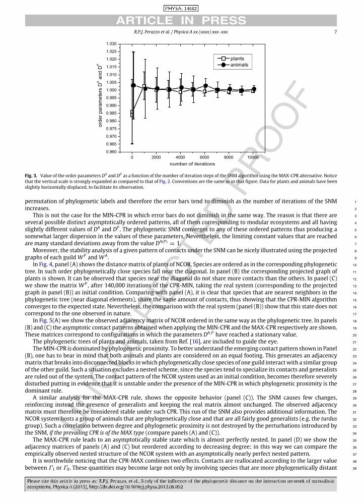
The ordered pattern that prevails asymptotically for the MAX-CPR case is a single, perfectly nested pattern. After some30

initial fluctuationsDA,P stabilize very closely to 1. The ordered pattern turns out to be essentially unique except for a random31

R.P.J. Perazzo et al. / Physica A xx (xxxx) xxx–xxx 7

Fig. 3. Value of the order parameters DA and DP as a function of the number of iteration steps of the SNM algorithm using theMAX-CPR alternative. Noticethat the vertical scale is strongly expanded as compared to that of Fig. 2. Conventions are the same as in that figure. Data for plants and animals have beenslightly horizontally displaced, to facilitate its observation.

permutation of phylogenetic labels and therefore the error bars tend to diminish as the number of iterations of the SNM 1

increases. 2

This is not the case for the MIN-CPR in which error bars do not diminish in the same way. The reason is that there are 3

several possible distinct asymptotically ordered patterns, all of them corresponding to modular ecosystems and all having 4

slightly different values of DA and DP . The phylogenetic SNM converges to any of these ordered patterns thus producing a 5

somewhat larger dispersion in the values of these parameters. Nevertheless, the limiting constant values that are reached 6

are many standard deviations away from the value DA(P)= 1. 7

Moreover, the stability analysis of a given pattern of contacts under the SNM can be nicely illustrated using the projected 8

graphs of each guildW P and W A. 9

In Fig. 4, panel (A) shows the distancematrix of plants of NCOR. Species are ordered as in the corresponding phylogenetic 10

tree. In such order phylogenetically close species fall near the diagonal. In panel (B) the corresponding projected graph of 11

plants is shown. It can be observed that species near the diagonal do not share more contacts than the others. In panel (C) 12

we show the matrix W P , after 140,000 iterations of the CPR-MIN, taking the real system (corresponding to the projected 13

graph in panel (B)) as initial condition. Comparing with panel (A), it is clear that species that are nearest neighbors in the 14

phylogenetic tree (near diagonal elements), share the same amount of contacts, thus showing that the CPR-MIN algorithm 15

converges to the expected state. Nevertheless, the comparison with the real system (panel (B)) show that this state does not 16

correspond to the one observed in nature. 17

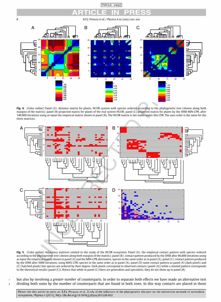
In Fig. 5(A) we show the observed adjacency matrix of NCOR ordered in the same way as the phylogenetic tree. In panels 18

(B) and (C) the asymptotic contact patterns obtained when applying theMIN-CPR and theMAX-CPR respectively are shown. 19

These matrices correspond to configurations in which the parameters DA,P have reached a stationary value. 20

The phylogenetic trees of plants and animals, taken from Ref. [16], are included to guide the eye. 21

TheMIN-CPR is dominated by phylogenetic proximity. To better understand the emerging contact pattern shown in Panel 22

(B), one has to bear in mind that both animals and plants are considered on an equal footing. This generates an adjacency 23

matrix that breaks into disconnected blocks inwhich phylogenetically close species of one guild interactwith a similar group 24

of the other guild. Such a situation excludes a nested scheme, since the species tend to specialize its contacts and generalists 25

are ruled out of the system. The contact pattern of the NCOR system used as an initial condition, becomes therefore severely 26

disturbed putting in evidence that it is unstable under the presence of the MIN-CPR in which phylogenetic proximity is the 27

dominant rule. 28

A similar analysis for the MAX-CPR rule, shows the opposite behavior (panel (C)). The SNM causes few changes, 29

reinforcing instead the presence of generalists and keeping the real matrix almost unchanged. The observed adjacency 30

matrix must therefore be considered stable under such CPR. This run of the SNM also provides additional information. The 31

NCOR system hosts a group of animals that are phylogenetically close and that are all fairly good generalists (e.g. the turdus 32

group). Such a correlation between degree and phylogenetic proximity is not destroyed by the perturbations introduced by 33

the SNM, if the prevailing CPR is of the MAX type (compare panels (A) and (C)). 34

The MAX-CPR rule leads to an asymptotically stable state which is almost perfectly nested. In panel (D) we show the 35

adjacency matrices of panels (A) and (C) but reordered according to decreasing degree; in this way we can compare the 36

empirically observed nested structure of the NCOR system with an asymptotically nearly perfect nested pattern. 37

It is worthwhile noticing that the CPR-MAX combines two effects. Contacts are reallocated according to the larger value 38

between Γ1 or Γ0. These quantities may become large not only by involving species that are more phylogenetically distant 39

8 R.P.J. Perazzo et al. / Physica A xx (xxxx) xxx–xxx

Fig. 4. (Color online) Panel (A): distance matrix for plants, NCOR system with species ordered according to the phylogenetic tree (shown along bothmargins of the matrix); panel (B):projected matrix for plants of the real system NCOR; panel (C):projected matrix for plants by the SNM MIN-CPR, after140,000 iterations using as input the empirical matrix shown in panel (B). The NCORmatrix is not stable under this CPR. The axes order is the same for thethree matrices.

A B

C D

Fig. 5. (Color online) Adjacency matrices related to the study of the NCOR ecosystem. Panel (A): the empirical contact pattern with species orderedaccording to the phylogenetic tree (shown along both margins of the matrix); panel (B): contact pattern produced by the SNM after 80,000 iterations usingas input the empirical matrix shown in panel (A) and theMIN-CPR alternative, species in the same order as in panel (A); panel (C): contact pattern producedby the SNM after 5000 iterations, using MAX-CPR, species in the same order as in panel (A); panel (D) same contact pattern as panel (A) (dark pixels) and(C) (hatched pixels) but species are ordered by their degree. Dark pixels correspond to observed contacts (panel (A)) while a slanted pattern correspondsto the theoretical results (panel (C)). Notice that while in panel (C) there are generalists and specialists, they do not show up in panel (B).

but also by involving a greater number of counterparts. In order to separate both effects we have made an alternative test1

dividing both sums by the number of counterparts that are found in both rows. In this way contacts are placed in those2

R.P.J. Perazzo et al. / Physica A xx (xxxx) xxx–xxx 9

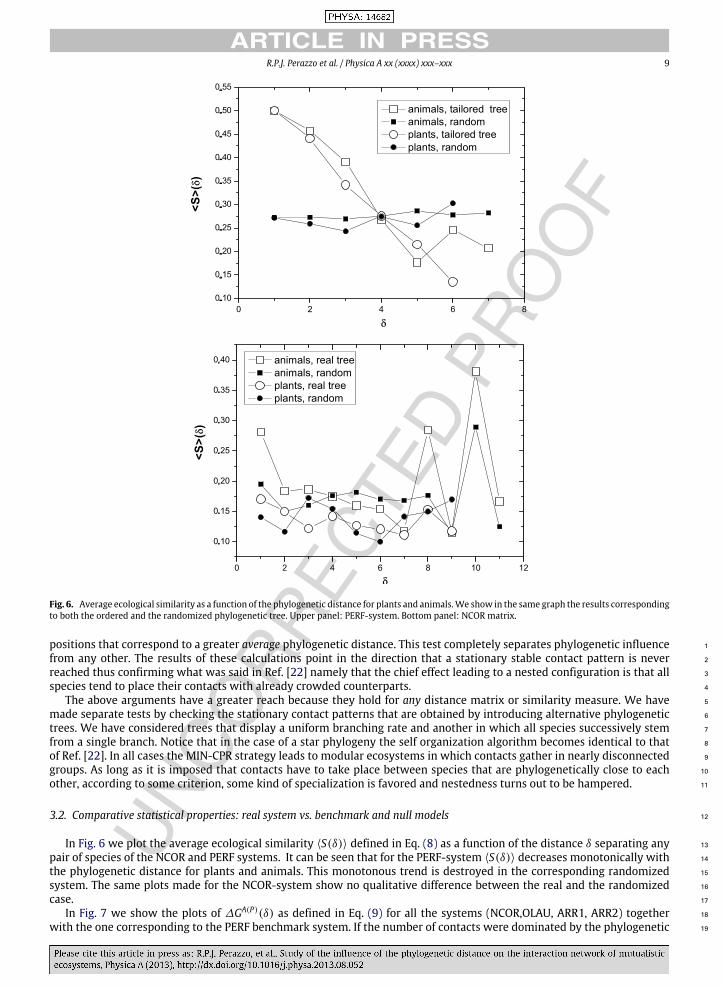
Fig. 6. Average ecological similarity as a function of the phylogenetic distance for plants and animals.We show in the same graph the results correspondingto both the ordered and the randomized phylogenetic tree. Upper panel: PERF-system. Bottom panel: NCOR matrix.

positions that correspond to a greater average phylogenetic distance. This test completely separates phylogenetic influence 1

from any other. The results of these calculations point in the direction that a stationary stable contact pattern is never 2

reached thus confirming what was said in Ref. [22] namely that the chief effect leading to a nested configuration is that all 3

species tend to place their contacts with already crowded counterparts. 4

The above arguments have a greater reach because they hold for any distance matrix or similarity measure. We have 5

made separate tests by checking the stationary contact patterns that are obtained by introducing alternative phylogenetic 6

trees. We have considered trees that display a uniform branching rate and another in which all species successively stem 7

from a single branch. Notice that in the case of a star phylogeny the self organization algorithm becomes identical to that 8

of Ref. [22]. In all cases the MIN-CPR strategy leads to modular ecosystems in which contacts gather in nearly disconnected 9

groups. As long as it is imposed that contacts have to take place between species that are phylogenetically close to each 10

other, according to some criterion, some kind of specialization is favored and nestedness turns out to be hampered. 11

3.2. Comparative statistical properties: real system vs. benchmark and null models 12

In Fig. 6 we plot the average ecological similarity ⟨S(δ)⟩ defined in Eq. (8) as a function of the distance δ separating any 13

pair of species of the NCOR and PERF systems. It can be seen that for the PERF-system ⟨S(δ)⟩ decreases monotonically with 14

the phylogenetic distance for plants and animals. This monotonous trend is destroyed in the corresponding randomized 15

system. The same plots made for the NCOR-system show no qualitative difference between the real and the randomized 16

case. 17

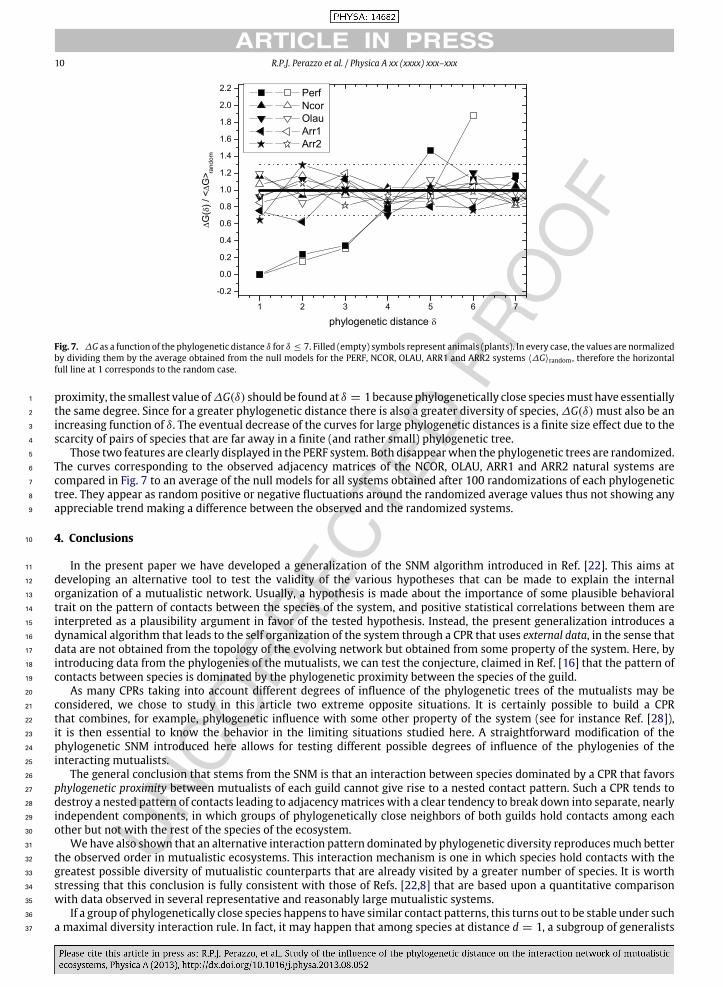
In Fig. 7 we show the plots of ∆GA(P)(δ) as defined in Eq. (9) for all the systems (NCOR,OLAU, ARR1, ARR2) together 18

with the one corresponding to the PERF benchmark system. If the number of contacts were dominated by the phylogenetic 19

10 R.P.J. Perazzo et al. / Physica A xx (xxxx) xxx–xxx

Fig. 7. ∆G as a function of the phylogenetic distance δ for δ ≤ 7. Filled (empty) symbols represent animals (plants). In every case, the values are normalizedby dividing them by the average obtained from the null models for the PERF, NCOR, OLAU, ARR1 and ARR2 systems ⟨∆G⟩random , therefore the horizontalfull line at 1 corresponds to the random case.

proximity, the smallest value of∆G(δ) should be found at δ = 1because phylogenetically close speciesmust have essentially1

the same degree. Since for a greater phylogenetic distance there is also a greater diversity of species, ∆G(δ) must also be an2

increasing function of δ. The eventual decrease of the curves for large phylogenetic distances is a finite size effect due to the3

scarcity of pairs of species that are far away in a finite (and rather small) phylogenetic tree.4

Those two features are clearly displayed in the PERF system. Both disappearwhen the phylogenetic trees are randomized.5

The curves corresponding to the observed adjacency matrices of the NCOR, OLAU, ARR1 and ARR2 natural systems are6

compared in Fig. 7 to an average of the null models for all systems obtained after 100 randomizations of each phylogenetic7

tree. They appear as random positive or negative fluctuations around the randomized average values thus not showing any8

appreciable trend making a difference between the observed and the randomized systems.9

4. Conclusions10

In the present paper we have developed a generalization of the SNM algorithm introduced in Ref. [22]. This aims at11

developing an alternative tool to test the validity of the various hypotheses that can be made to explain the internal12

organization of a mutualistic network. Usually, a hypothesis is made about the importance of some plausible behavioral13

trait on the pattern of contacts between the species of the system, and positive statistical correlations between them are14

interpreted as a plausibility argument in favor of the tested hypothesis. Instead, the present generalization introduces a15

dynamical algorithm that leads to the self organization of the system through a CPR that uses external data, in the sense that16

data are not obtained from the topology of the evolving network but obtained from some property of the system. Here, by17

introducing data from the phylogenies of the mutualists, we can test the conjecture, claimed in Ref. [16] that the pattern of18

contacts between species is dominated by the phylogenetic proximity between the species of the guild.19

As many CPRs taking into account different degrees of influence of the phylogenetic trees of the mutualists may be20

considered, we chose to study in this article two extreme opposite situations. It is certainly possible to build a CPR21

that combines, for example, phylogenetic influence with some other property of the system (see for instance Ref. [28]),22

it is then essential to know the behavior in the limiting situations studied here. A straightforward modification of the23

phylogenetic SNM introduced here allows for testing different possible degrees of influence of the phylogenies of the24

interacting mutualists.25

The general conclusion that stems from the SNM is that an interaction between species dominated by a CPR that favors26

phylogenetic proximity between mutualists of each guild cannot give rise to a nested contact pattern. Such a CPR tends to27

destroy a nested pattern of contacts leading to adjacencymatrices with a clear tendency to break down into separate, nearly28

independent components, in which groups of phylogenetically close neighbors of both guilds hold contacts among each29

other but not with the rest of the species of the ecosystem.30

Wehave also shown that an alternative interaction pattern dominated by phylogenetic diversity reproducesmuch better31

the observed order in mutualistic ecosystems. This interaction mechanism is one in which species hold contacts with the32

greatest possible diversity of mutualistic counterparts that are already visited by a greater number of species. It is worth33

stressing that this conclusion is fully consistent with those of Refs. [22,8] that are based upon a quantitative comparison34

with data observed in several representative and reasonably large mutualistic systems.35

If a group of phylogenetically close species happens to have similar contact patterns, this turns out to be stable under such36

a maximal diversity interaction rule. In fact, it may happen that among species at distance d = 1, a subgroup of generalists37

R.P.J. Perazzo et al. / Physica A xx (xxxx) xxx–xxx 11

Fig. 8. An example of a simple phylogenetic tree is shown. The matrix of distances is: d(1, 2) = d(4, 5) = 1 d(1, 3) = d(1, 4) = d(1, 5) = d(2, 3) =

d(2, 4) = d(2, 5) = 3 d(3, 4) = d(3, 5) = 2.

(as is the case of the turdus group in the NCOR system) might be found. In this case such a subgroup will remain stable 1

under the organization algorithm of the SNM-MAX. This does not mean that all species at distance d = 1, will have a similar 2

degree. 3

These results place serious doubts on the fact of considering the correlations between degree distributions and 4

phylogenetic proximity as a sign of causation. The few circumstances in which they have been found to be statistically 5

significant [16,18], point to the direction of considering that these are largely accidental, i.e. due to the existence of some 6

phylogenetically related generalists. 7

The comparison of statistical studies performed on the real networks with those performed on a benchmark ideal model 8

and on a null model, are compatible with the results issued from the phylogenetic SNM. 9

A dominant cause of the generalized nestedness found in mutualistic ecosystems lies perhaps on the simple fact that 10

species that we observe in real systems today are those that tend to put the least possible restrictions on their mutualistic 11

counterparts. 12

Acknowledgment 13

The authors wish to acknowledge helpful discussions and criticism from D. Medan and M. Devoto. 14

Appendix. The distance matrix 15

If a tree-like diagram is provided it is possible to extract from it a square matrix d(k, k′) of all distances between any two 16

living species k and k′. One biologically plausible way to define such distance is to extract it from their evolutionary history. 17

This amounts to considering that two species are ‘‘separated by a distance’’ that is measured by the time elapsed since they 18

were differentiated in the course of evolution. 19

The evolutionary time can be represented by the length of the branches of the tree. 20

Resemblances and differences measured by this distance could be considered to involve a compound effect of all the 21

traits that where considered in the analyses that led to the phylogenetic tree. 22

In order to obtain the distance matrix with all the distances one has to provide a uniform time scale for all branches, 23

i.e., to provide a time order for all the branching points of the phylogenetic tree. The most parsimonious way of doing this is 24

by defining that all branches that stem from a common ancestor and reach the tips of the tree must have the same length, 25

counting lengths by starting from the tips and climbing upwards. This assumption is consistent with the constancy of an 26

evolutionary clock [29]. 27

With this procedure the distance matrix can directly be read from the topology of the phylogenetic tree. We exemplify 28

this procedure in Fig. 8. We define that the two branches that lead to the species labeled (4) and (5) having a common 29

ancestor in node (A) have a length equal to 1. By the same rule, the branch starting at species (3) that has a common ancestor 30

with (4) and (5) in the branchpoint (B) has a length equal to 2. Moreover, the total length of the branches that have to be 31

climbed starting from (1) or (2) to reach a common ancestor to all species in (C) must then have a total length of 3. In all 32

these cases the lengths are defined except for an overall multiplicative scale factor. This ambiguity is however not relevant 33

for the present analysis. 34

References 35

[1] C.M. Herrera, O. Pellmyr (Eds.), Plant-animal Interactions. An Evolutionary Approach, Blackwell Science, Oxford, 2002. 36

[2] N. Waser, J. Ollerton (Eds.), Plant–pollinator Interactions. From Specialization to Generalization, University of Chicago Press, Chicago, 2006. 37

[3] J. Memmott, N.M. Waser, M.V. Price, Tolerance of pollination networks to species extinctions, Proc. R. Soc. Lond. B (271) (2004) 2605–2611. 38

[4] D.Medan, N.H.Montaldo, M. Devoto, A. Mantese, V. Vasellati, G.G. Roitman, N.H. Bartoloni, Plant–pollinator relationships at two altitudes in the Andesof Mendoza, Argentina. Arctic, Antarctic and Alpine Research (ISSN: 1523-0430) 34 (2002) 233–241.

39

[5] R.F. Clements, F.L. Long, Experimental Pollination. An Outline of the Ecology of Flowers and Insects, Carnegie Institute of Washington, Washington,1923.

40

[6] C. Robertson, Flowers and Insects: Lists of Visitors to Four Hundred and Fifty-Three Flowers, C. Robertson, Carlinville, IL., 1929. 41

12 R.P.J. Perazzo et al. / Physica A xx (xxxx) xxx–xxx

[7] M. Kato, T. Makutani, T. Inoue, T. Itino, Insect-flower relationship in the primary beech forest of Ashu, Kyoto: an overview of the flowering phenologyand seasonal pattern of insect visits, Contr. Biol. Lab. Kyoto Univ. 27 (1990) 309–375.

1

[8] E. Burgos, H. Ceva, R.P.J. Perazzo, M. Devoto, D. Medan, M. Zimmermann, A.M. Delbue, J. Theoret. Biol. 249 (2007) 307.2

[9] J. Bascompte, P. Jordano, C.J. Melián, J.M. Olesen, Proc. Natl. Acad. Sci. USA 100 (2003) 9383–9387;3

P. Jordano, J. Bascompte, and J.M. Olesen N. Waser and J. Ollerton (Eds.), University of Chicago Press (2006) 173–199.4

[10] J. Memmott, N.M. Waser, M.V. Price, Proc. R. Soc. B 271 (2004) 2605;5

J. Memmott, D. Alonso, E.L. Berlow, A. Dobson, J.A. Dunne, R. Solé, J. Weitz, J. Pascual, M. Dunne, J.A. (Eds.), Ecological Networks: Linking Structure toDynamics in Food Webs, Oxford University Press, New York, 2005, p. 325.

6

[11] César Hidalgo, Ricardo Hausmann, Proc. Natl. Acad. Sci. USA 106 (2009) 10570–10575.7

[12] Sebastián Bustos, Charles Gomez, Ricardo Hausmann, César Hidalgo, PLOS ONE 7 (2012) e49393.8

[13] Guido Caldarelli, Matthieu Cristelli, Andrea Gabrielli, Luciano Pietronero, Antonio Scala, Andrea Tacchella, PLOS ONE 7 (2012) e47278.9

[14] L. Ermann, D.L. Shepelyansky, Phys. Lett. A 377 (2013) 250–256.10

[15] P. Jordano, J. Bascompte, J.M. Olesen, Ecology Lett. 6 (2003) 69.11

[16] E.L. Rezende, J.E. Lavabre, P.R. Guimaraes, Jr., P. Jordano, J. Bascompte, Nature 448 (2007) 925.12

[17] E.L. Rezende, P. Jordano, J. Bascompte, Oikos 116 (2007) 1919.13

[18] Susanne S. Renner, Nature 448 (2007) 877.14

[19] D.P. Vázquez, M.A. Aizen, N. Waser, and J. Ollerton (Eds.), University of Chicago Press, Chicago, (2006), p. 112.Q315

[20] M. Stang, P.G.L. Klinkhamer, E.van der Meijden, visitor web Oikos 112 (2006) 111–121.16

[21] D.P. Vazquez, N.P. Chacoff, L. Cagnolo, Ecology 90 (2009) 2039.17

[22] D. Medan, R.P.J. Perazzo, M. Devoto, E. Burgos, M. Zimmermann, H. Ceva, A.M. Delbue, J. Theoret. Biol. 246 (2007) 510.18

[23] E. Burgos, H. Ceva, L. Hernández, R.P.J. Perazzo, M. Devoto, D. Medan, Phys. Rev. E78 (2008) 046113.19

[24] M.E.J. Newman, S.H. Strogatz, D.J. Watts, Phys. Rev. E 64 (2001) 026128.20

[25] A.L. Barabási, R. Albert, Science 286 (1999) 500.21

[26] J. Felsestein, Amer. Nat. 125 (1985) 1.22

[27] S.P. Blomberg, T. Garland, A.R. Ives, Evolution 57 (4) (2003) 717.23

[28] A.R. Ives, H.C.J. Godfray, Amer. Nat. 168 (2006) E1.24

[29] M. Kimura M, New Sci. 107 (N1464) (1985) 41.25