Embed Size (px)
Citation preview
1
Study of Spontaneous Polymerisation Inhibition
Thomas Edward Newby
PhD
University of York
Chemistry
May 2014
2
Abstract
Spontaneous polymerisation is an unwanted reaction, prevented by inhibitor molecules. In
order to observe the inhibition of spontaneous polymerisation by different molecules, a
small scale dilatometry experiment was developed. This was used to screen structurally
related molecules to 2-nitrophenol to determine what structural features give rise to
inhibition properties. Compounds with an intramolecular hydrogen bond demonstrated
more efficient inhibition of polymerisation.
The product mixture of styrene inhibited by 2-nitrophenol was analysed to determine the
reaction pathway. Column chromatography, MS and NMR were used to determine the
structure of two intermediates, 2-aminophenol and a compound derived from a Diels Alder
styrene initiator and 2-nitrophenol.
The proposed intermediate, 2-nitrosophenol, was synthesised and its stability in styrene
was determined. The products of reaction between 2-nitrosophenol and styrene at room
temperature were proposed by comparing results with the reaction between styrene and
nitrosobenzene. The main product of the inhibition by 2-nitrosophenol, was also
determined to be 2-aminophenol, suggesting that 2-aminophenol formed from inhibition
by 2-nitrophenol goes via 2-nitrosophenol.
Other intermediates and products identified were also screened in the dilatometry setup.
They show inhibition properties at high concentration, but at more realistic concentrations,
they did not inhibit styrene polymerisation. An overall mechanism for the inhibition of
styrene polymerisation by 2-nitrophenol, was proposed based on the data obtained.
3
Contents
Abstract .................................................................................................................................... 2
Contents ................................................................................................................................... 3
List of figures ........................................................................................................................ 9
List of schemes ................................................................................................................... 15
List of tables ....................................................................................................................... 18
List of equations ................................................................................................................. 20
Acknowledgments .................................................................................................................. 21
Authors declaration ............................................................................................................... 23
1. Introduction ................................................................................................................... 24
1.1 Properties of a polymer ......................................................................................... 24
1.2 Radical polymerisation ........................................................................................... 27
1.2.1 Spontaneous polymerisation ......................................................................... 30
1.2.1.1 Bi-radical mechanism ................................................................................. 30
1.2.1.2 Pericyclic mechanisms ............................................................................... 32
1.2.1 Living radical polymerisation ......................................................................... 34
1.3 Inhibition of polymerisation................................................................................... 36
1.3.1 Direct reaction with initiator radical .............................................................. 37
1.3.1.1 Oxygen ....................................................................................................... 37
1.3.1.2 Stable radicals ............................................................................................ 38
1.3.1.3 Nitroaromatics and nitrophenols ............................................................... 39
1.3.1.4 Quinones .................................................................................................... 41
1.3.1.5 Phenothiazine ............................................................................................ 42
1.3.2 Reactions of inhibitors with peroxyl radicals ................................................. 43
1.3.2.1 Phenolics .................................................................................................... 43
1.4 Electron paramagnetic resonance ......................................................................... 44
4
1.4.1 Basic principle – Zeeman Splitting ................................................................. 45
1.4.2 Instrumentation and Detection ..................................................................... 46
1.4.2.1 Noise reduction and sensitivity .................................................................. 47
1.4.3 Analysis and interpretation of spectra ........................................................... 47
1.4.3.1 Hyperfine interactions ............................................................................... 48
1.4.3.2 Intensity ..................................................................................................... 49
1.4.3.3 Line broadening ......................................................................................... 49
1.5 Aims of the study ................................................................................................... 50
2. Nitrophenols as inhibitors .............................................................................................. 51
2.1 Monitoring polymerisation .................................................................................... 51
2.2 Dilatometry ............................................................................................................ 54
2.2.1 Disadvantages of current methods ................................................................ 56
2.3 Design of a new and automated dilatometry experiment .................................... 57
2.3.1 Rack ................................................................................................................ 58
2.3.2 Oil bath and heating ....................................................................................... 60
2.3.3 Sample preparation ....................................................................................... 61
2.3.4 Camera and lighting ....................................................................................... 62
2.3.5 Data analysis .................................................................................................. 62
2.3.6 Standards and calibration of the new setup .................................................. 63
2.3.7 Oxygen diffusion within the samples ............................................................. 64
2.4 Case studies for proof of concept .......................................................................... 67
2.4.1 Uninhibited styrene ....................................................................................... 67
2.4.2 Nitroxide inhibited polymerisation (TEMPO) ................................................. 68
2.4.3 Oxygen dependent inhibitor (4-methoxyphenol) .......................................... 70
2.4.4 Conclusions on the new dilatometry set-up .................................................. 71
2.5 Dilatometry study of the inhibition properties of ortho-nitrophenols and related
compounds ........................................................................................................................ 72
2.5.1 DNBP, 2,4-dinitrophenol and 2-nitrophenol .................................................. 72
5
2.5.2 2-Nitrophenol, 3-nitrophenol and 4-nitrophenol .......................................... 74
2.5.3 The structural group responsible for inhibition ............................................. 76
2.5.4 Nitroanilines ................................................................................................... 80
2.5.5 Nitroanisole (removing the hydrogen bond to the nitro group) ................... 82
2.5.6 2-Nitroacetanilide and 2-nitrotrifluoroacetanilide ........................................ 83
2.6 Conclusions from the dilatometry screening experiment ..................................... 85
3. Nitrophenols as inhibitors – Product analysis................................................................ 87
3.1 Introduction ........................................................................................................... 87
3.2 MS analysis of inhibition product mixture ............................................................. 88
3.3 GC and GC / MS analysis of inhibition product mixture ........................................ 90
3.4 Identification of reactive intermediates by EPR .................................................... 94
3.5 Isolation and identification of Unknown A and Unknown B .................................. 96
3.5.1 Acid / Base extraction .................................................................................... 97
3.5.2 Methanol precipitation .................................................................................. 99
3.5.3 Column chromatography ............................................................................. 100
3.5.4 Polymer precipitation by methanol and water ............................................ 102
3.6 Structure determination of unknown B by NMR ................................................. 104
3.6.1 Degree of unsaturation ................................................................................ 115
3.7 X-ray crystallography of isolated unknown B ...................................................... 116
3.8 Possible mechanism for the formation of Unknown B ........................................ 119
3.9 Synthesis of the unknown B ................................................................................. 121
3.9.1 Ketone intermediate (Compound D) ........................................................... 121
3.9.2 Synthesis of deuterated compound D. ........................................................ 127
3.9.3 Synthesis of imine (Compound E) ................................................................ 128
3.9.4 Final cyclisation to compound C .................................................................. 130
4. Intermediates in the inhibition of spontaneous polymerisation of styrene by
nitrophenols ......................................................................................................................... 134
4.1 Further dilatometry ............................................................................................. 135
6
4.1.1 2-Aminophenol ............................................................................................ 135
4.1.2 Imines as inhibitors ...................................................................................... 138
4.1.3 Unknown B as an inhibitor ........................................................................... 142
4.1.4 2-Nitrosophenol ........................................................................................... 143
4.2 Further product analysis ...................................................................................... 145
4.2.1 Nitroso intermediates .................................................................................. 145
4.2.1.1 Nitrosobenzene ........................................................................................ 145
4.2.1.2 2-Nitrosophenol ....................................................................................... 149
4.2.2 EPR of 2-nitrosophenol in styrene ............................................................... 154
4.3 Conclusions from the additional dilatometry and product analysis .................... 156
4.4 The Mechanism of Inhibition ............................................................................... 157
4.4.1 Is inhibition stoichiometric or catalytic? ...................................................... 157
4.4.2 Reactions with the initiator radical .............................................................. 159
4.5 Conclusion ............................................................................................................ 162
5. Chloranil Radical Anion ................................................................................................ 163
5.1 Introduction ......................................................................................................... 163
5.1.1 A new inhibitor ............................................................................................. 163
5.1.2 Aims .............................................................................................................. 166
5.2 Chloranil Radical Anion Stability in aqueous solution ......................................... 167
5.2.1 Products from the decomposition of chloranil radical anion potassium salt.
169
5.2.2 Chloranil radical anion potassium salt under nitrogen ................................ 174
5.2.3 Lack of reproducibility .................................................................................. 175
5.2.4 Conclusions .................................................................................................. 180
5.3 Comproportionation / disproportionation equilibrium ....................................... 181
5.3.1 Chemical exchange of 2,5 – di-tert-butyl semiquinone in concentrated
solutions of 2,5 – di-tert-butyl hydroquinone ............................................................. 183
7
5.3.2 Equilibrium constants of the comproportionation / disproportionation
equilibrium of 2,5 – di-tert-butyl hydroquinone and 2,5 – di-tert-butylquinone in polar
media 185
5.3.3 Sensitivity of disproportionation/comproportionation equilibrium to
reaction conditions ...................................................................................................... 192
5.3.4 The comproportionation / disproportionation equilibrium in apolar media
195
5.4 Conclusions .......................................................................................................... 202
6. Final conclusions .......................................................................................................... 204
7. Experimental ................................................................................................................ 206
7.1 Chemicals and materials ...................................................................................... 206
7.1.1 Styrene preparation ..................................................................................... 206
7.2 NMR ..................................................................................................................... 206
7.3 EPR ....................................................................................................................... 207
7.4 MS ........................................................................................................................ 207
7.5 Dilatometry .......................................................................................................... 207
7.6 Oximetry (Oxygen diffusion into chlorobenzene) ................................................ 208
7.7 Column Chromatography / Thin Layer Chromatography .................................... 208
7.8 X-ray crystallography ........................................................................................... 208
7.9 Synthesis .............................................................................................................. 209
7.9.1 Chloranil radical anion potassium salt synthesis ......................................... 209
7.9.2 2-nitrosophenol synthesis ............................................................................ 210
7.9.3 Unknown B isolation .................................................................................... 210
7.9.4 Compound C synthesis – ketone precursor (Compound D) ......................... 211
7.9.5 Synthesis of Compound E ............................................................................ 212
7.9.6 Compound E to Compound C reaction ........................................................ 213
7.9.7 N-(1-Phenylethylene)-o-aminophenol – Compound F................................. 213
8. Appendices ................................................................................................................... 215
8.1 Glossary ................................................................................................................ 233

8
9. References ................................................................................................................... 234

9
List of figures
Figure 1. Relationship between chain length of a polymer and its properties; viscosity,
tensile and impact strength ................................................................................................... 26
Figure 2. Relationship between the elastic properties of a polymer and its degree of cross-
linkage .................................................................................................................................... 26
Figure 3. Dimers and trimers found after the self-polymerisation of methyl methacrylate.
Two other dimers were observed but could not be characterised due to low quantities .... 33
Figure 4. The difference in energy levels caused by Zeeman splitting ................................. 45
Figure 5. The hyperfine splitting of an unpaired electron interacting with an 15N nucleus, in
a magnetic field, B. ................................................................................................................. 48
Figure 6. EPR spectra of TEMPO (Left) and 2,5 – di-tert-butyl semiquinone(Right) ............. 49
Figure 7. Diagram of a basic dilatometry set-up ................................................................... 53
Figure 8. Schematic and digital render of the dilatometry rack. Dimensions, where given,
are in millimetres .................................................................................................................. 59
Figure 9. Photo of the dilatometry rack with features labelled ............................................ 59
Figure 10. Temperature equilbration of dilatomemtry sample. Sample inserted into heated
oil bath at time = 20 seconds ................................................................................................. 61
Figure 11. Dilatometry of toluene, as a demonstration of the equipment stability. Data
normalized to the first image taken at t = 0 minutes. ........................................................... 64
Figure 12. The oxygen diffusion into chlorobenzene at 100°C, monitored by EPR .............. 65
Figure 13. A comparison between the oxygen consumption by styrene polymerisation and
the oxygen diffusion into chlorobenzene. (At 100°C, monitored by EPR) ............................ 66
Figure 14. Dilatometry of uninhibited styrene at 110°C ....................................................... 68
Figure 15. 200ppm TEMPO in styrene polymerisation measured by the dilatometry set-up
at 110°C .................................................................................................................................. 69
Figure 16. Inhibition period against TEMPO concentration .................................................. 69
Figure 17. 3 dilatometry samples of 100ppm MEHQ in styrene polymerisation at 90°C ..... 70
Figure 18 Dilatometry trace of uninhibited styrene, 0.1M DNBP, 0.1M 2,4-dinitrophenol,
and 0.1M 2-nitrophenol (in styrene) at 110 °C. ..................................................................... 73
Figure 19 Dilatometry traces of styrene, 0.1 M 2-nitrophenol, 0.1 M 3-nitrophenol and 0.1
M 4-nitrophenol (in styrene) at 110 °C. ................................................................................. 75
10
Figure 20. Contour plot of the isotropic chemical shielding (ppm) through the molecular
plane of 2-nitrophenol (a) and 4-nitrophenol (b) calculated at the MP2/6-311++G(d,p) level
of theory................................................................................................................................. 79
Figure 21. Demonstration of difference in bond order of the nitro group without hydrogen
bonding (Left) and with hydrogen bonding (Right) ............................................................... 80
Figure 22. 2-Nitroaniline, 3-nitroaniline and 4-nitroaniline................................................... 80
Figure 23 Dilatometry of styrene, 0.1 M 2-nitrophenol, 0.1 M 2-nitroaniline and 0.1 M 3-
nitroaniline (in styrene) at 110 °C. ......................................................................................... 81
Figure 24. 2-Nitroanisole, 3-nitroanisole and 4-nitroanisole ................................................. 82
Figure 25. Dilatometry of styrene, 0.1M 2-, 3- and 4-nitroanisole (in styrene) at 110 °C. ... 82
Figure 26. 2-Nitroacetanilide and 2-nitrotrifluoroacetanilid ................................................ 83
Figure 27. Dilatometry traces of styrene, 0.1 M 2-nitroacetanilide and 0.1 M 2-
nitrotrifluoroacetanilide (in styrene) at 110 °C. ..................................................................... 84
Figure 28. Dilatometry trace for 3 mmol 2-nitrophenol and 2-nitroacetanilide inhibited
styrene at 110°C. .................................................................................................................... 85
Figure 29. ESI MS of the high concentration 2-nitrophenol inhibition mixture. ................... 89
Figure 30. ESI MS of the high concentration 2-nitrophenol inhibition mixture heated for 8
days, until it became too viscous. .......................................................................................... 89
Figure 31. Gas chromatogram of 0.01M 2-nitrophenol in styrene heated at 110°C for 24
hours. Sample was split 50:1 at the injection. ...................................................................... 91
Figure 32. Gas chromatogram of 0.01M 2-nitrophenol in styrene heated at 110°C for 24
hours. Sample was not split, but detector was deactivated for the first 5 minutes of the
chromatogram. ...................................................................................................................... 92
Figure 33. 0.1M 2-nitrophenol in styrene at 130°C, average of 40 spectra. ......................... 95
Figure 34. ESI MS of the acid extract (Black) and the neutral organic solution (Blue) .......... 98
Figure 35. H1 NMR of acid extract (Unknown A) in blue and 2-aminophenol in red. (400
MHz, CDCl3) ............................................................................................................................ 99
Figure 36. H1 NMR of reaction mixture without any separation. (400 MHz, CDCl3) ........... 100
Figure 37. MS of fraction containing unknown B (Rf = 0.33). ............................................. 101
Figure 38. H1 NMR of the first successful isolation of unknown B. (400 MHz, CDCl3) ........ 102
Figure 39. H1 NMR of isolated unknown B after water/methanol isolation. (400 MHz, CDCl3)
............................................................................................................................................. 103
Figure 40. 1H NMR of unkown B, low field. (700 MHz, CDCl3) ............................................ 105
Figure 41. 1H NMR of unknown B, high field. (700 MHz, CDCl3) ........................................ 105
11
Figure 42. COSY spectrum of unknown B. (700 MHz, CDCl3) The aromatic and non-
aromatic protons have been boxed to distinguish the different types of protons. ............ 106
Figure 43. NMR of Unknown B. Close up proton of non-aromatic protons (700 MHz, CDCl3)
............................................................................................................................................. 107
Figure 44. Proposed structure for fragment A .................................................................... 107
Figure 45. Fragment A, with coupling constants assigned.................................................. 109
Figure 46. The proposed structure for fragment B. ............................................................ 109
Figure 47. Close-up of protons C, E and H. (700 MHz, CDCl3) ............................................. 110
Figure 48. Close-up of protons B, F, G and I. (700 MHz, CDCl3) ........................................... 111
Figure 49. The proposed structure for fragment C. ............................................................ 112
Figure 50. The proposed structure for fragment D. ............................................................ 113
Figure 51. Fragment A, with HMBC couplings shown. Couplings common to protons K, L
and M are in red, and those common to protons J, L and M are in blue. ........................... 113
Figure 52. The proposed structure and assignment of unknown B. ................................... 115
Figure 53. X-ray crystallography results of a sample of unknown B, crystallised from CDCl3.
............................................................................................................................................. 116
Figure 54. Comparison between 2-nitrophenol, unknown B and the spontaneous
polymerisation initiator proposed by Mayo19...................................................................... 119
Figure 55. NMR of compound D, low field. (400 MHz, CDCl3) ............................................ 124
Figure 56. NMR of compound D, high field. (400 MHz, CDCl3) ........................................... 124
Figure 57. Structure assignment for compound D .............................................................. 127
Figure 58. H1 NMR of ketone intermediate, synthesised using deuterated benzene. (400
MHz, CDCl3) .......................................................................................................................... 128
Figure 59. ESI MS of compound E mixture isolated. ........................................................... 129
Figure 60. H1 NMR of compound E mixture, magnified on high field signals. (400 MHz,
CDCl3) ................................................................................................................................... 129
Figure 61. MS spectrum of final synthesis step after 1 hour .............................................. 131
Figure 62 MS spectrum of final synthesis step after 4 hours.............................................. 131
Figure 63 MS/MS of peak m/z 312 comparisons between inhibited polymerisation mixture
(top) and isolated unknown B (bottom) .............................................................................. 132
Figure 64. Dilatometry of styrene and styrene inhibited by 0.1 M 2-aminophenol at 110°C
............................................................................................................................................. 136
Figure 65. Dilatometry traces of styrene, 0.1 M 2-aminophenol in styrene and 0.1 M 2-
amino-4-sec-butylphenol in styrene at 110°C ..................................................................... 137

12
Figure 66. Dilatometry of styrene, and styrene inhibited by 3 mM 2-nitrophenol and 3 mM
2-aminophenol at 110°C. ..................................................................................................... 138
Figure 67. Dilatometry traces of styrene, and styrene inhibited by 0.1 M compound B at
110°C .................................................................................................................................... 140
Figure 68. Dilatometry of uninhibited styrene and styrene inhibited by 0.1M compound F
at 110°C. ............................................................................................................................... 141
Figure 69. Dilatometry of styrene and styrene inhibited by 2-nitrophenol , 2-aminophenol,
compound E or compound F (3 mM) at 110°C. ................................................................... 142
Figure 70. Dilatometry of styrene inhibited by 0.1 M unknown B at 110°C ....................... 143
Figure 71. Dilatometry of styrene and styrene inhibited by 0.1 M 2-nitrosophenol at 110°C.
............................................................................................................................................. 144
Figure 72. Dilatometry trace styrene inhibited with 3 mmol 2-nitrophenol and 3 mmol 2-
nitrosophenol at 110°C. ....................................................................................................... 144
Figure 73. Dilatometry traces of styrene and 0.1 M nitrosobenzene prepared fresh and
aged for 24 hours at room temperature. Dilatometry performed at 110°C. ..................... 147
Figure 74. MS of sample of nitrosobenzene in styrene, analysed immediately ................. 148
Figure 75. MS of sample of nitrosobenzene in styrene, analysed after 24 hours at room
temperature ......................................................................................................................... 148
Figure 76. H1 NMR of the reaction mixture between nitrosobenzene and styrene after
solvent removal. (400 MHz, CDCl3) ...................................................................................... 149
Figure 77. MS of 0.1M 2-nitrosophenol in styrene after 24 hours ..................................... 150
Figure 78. MS of the products of styrene spontaneous polymerisation inhibited by 0.1 M 2-
nitrosophenol. ...................................................................................................................... 152
Figure 79. MS of product mixture of 0.1M 2-nitrosophenol in methyl styrene, heated at
110°C for 5 hours ................................................................................................................. 153
Figure 80. EPR of 2-nitrosophenol in styrene, average of spectra taken 35-55 minutes after
addition (Black line) and a simulation of the proposed radical formed (Red line). ............. 155
Figure 81. The amount of radical formed during spontaneous initiation of styrene at 110
°C. ......................................................................................................................................... 159
Figure 82. Rate of decomposition of chloranil radical anion potassium salt, as observed
from the EPR intensity. The first spectrum was not taken at t = 0 minutes, as the
equipment can only be tuned once the sample is prepared and in the equipment ........... 168
Figure 83 Negative ion ESI mass spectra of the decay products for chloranil radical anion in
water, open to air at room temperature. ............................................................................ 170
13
Figure 84. Magnification of isotope pattern for peak A in blue, with the calculated isotope
pattern in red. ...................................................................................................................... 170
Figure 85 Decay of chloranil radical anion in water under nitrogen environment, as
observed from the EPR intensity ......................................................................................... 174
Figure 86. Comparison of the rates of decay under nitrogen (Blue) and open to air (Red).
............................................................................................................................................. 175
Figure 87. EPR signal decay for chloranil radical anion in deionised water. ....................... 176
Figure 88. Normalised EPR signal intensities for samples of batch 3 radical anion (100ppm)
in water ................................................................................................................................ 177
Figure 89. Decay of chloranil radical anion in water under nitrogen environment............ 178
Figure 90. Normalised EPR signal intensities for samples of batch 3 radical anion (100 ppm)
in water ................................................................................................................................ 178
Figure 91. Comparison of the rates of decay under nitrogen (Blue) and open to air (Red).
............................................................................................................................................. 179
Figure 92. EPR spectra for the formation of the chloranil radical anion from tetrachloro
hydroquinone, sodium hydroxide and chloranil, and combinations thereof ...................... 182
Figure 93. EPR spectra of di-tert-butyl hydroquinone in ethanol at different concentrations,
spectra normalised (1mM - Green, 10mM – Blue and 1M - Red) ...................................... 184
Figure 94. The results of three runs for the comproportionation / disproportionation
equilibrium at varying molar equivalents of quinone at -30°C ............................................ 188
Figure 95. The results of three runs for the comproportionation / disproportionation
equilibrium at varying molar equivalents of quinone at 0°C ............................................... 188
Figure 96. The results of three runs for the comproportionation / disproportionation
equilibrium at varying molar equivalents of quinone at 30°C ............................................. 189
Figure 97. The results of three runs for the comproportionation / disproportionation
equilibrium at varying molar equivalents of quinone at 60°C ............................................. 189
Figure 98. The effect of excess base on a 1:1 hydroquinone: quinone mixture in ethanol.
The concentration on the y-axis is the radical observed. .................................................... 193
Figure 99. EPR signal of 2,5-diterbutyl semiquinone radical anion in ethanol at room
temperature. ........................................................................................................................ 197
Figure 100. EPR signal of 2,5-diterbutyl semiquinone radical anion in THF at room
temperature ......................................................................................................................... 198
Figure 101. EPR signal of the 2,5-diterbutyl semiquinone radical anion in 2% ethanol /
toluene at -60°C ................................................................................................................... 199
14
Figure 102. 13C NMR 700MHz of 312 fraction, low field, in CDCl3. ..................................... 216
Figure 103. 13C NMR 700MHz of 312 fraction, high field, in CDCl3. .................................... 216
Figure 104. COSY spectra of compound B. (700MHz, CDCl3) ............................................. 217
Figure 105. HSQC spectra of compound B. (700MHz, CDCl3) ............................................. 218
Figure 106. HMBC spectra of compound B. (700MHz, CDCl3) ............................................ 219
Figure 107. MS of compound D synthesised following the procedure by Rendy et al100. .. 221
Figure 108. 13C NMR of the compound D. (400MHz, CDCl3) ............................................... 222
Figure 109. 13C NMR of the compound D, low field magnification. (400MHz, CDCl3) ........ 222
Figure 110. COSY spectra of compound D. (400MHz, CDCl3) .............................................. 223
Figure 111. HSQC spectra of compound D. (400MHz, CDCl3) ............................................. 224
Figure 112. HMBC spectra of compound D. (400MHz, CDCl3) ............................................ 225
Figure 113. NMR of compound E mixture. (400MHz, CDCl3) .............................................. 226
15
List of schemes
Scheme 1 Demonstration of tacticity of polymers3 ............................................................... 25
Scheme 2. Initiation and propagation steps in radical polymerisation ................................. 27
Scheme 3 Thermal activation of dicumyl peroxide initiator .................................................. 28
Scheme 4. Formation of a propagating radical mid chain in styrene polymerisation .......... 28
Scheme 5. The termination through recombination of radicals ........................................... 29
Scheme 6. Demonstration of disproportionation ................................................................. 29
Scheme 7. The initiation of vinyl monomers proposed by Hall11, 12 ....................................... 31
Scheme 8. The dimer bi-radical proposed by Flory10 for the initiator in the thermal
polymerisation of methyl methacrylate. ............................................................................... 31
Scheme 9. A mechanism dismissed by Flory for the formation of an initiator in the thermal
polymerisation of a vinyl compound. .................................................................................... 31
Scheme 10. The Mayo mechanism for the self-initiation of styrene18, 19 .............................. 32
Scheme 11. The dimerisaion of methyl methacrylate following Diels Alder self-addition
similar to that described by Mayo18, 19 ................................................................................... 33
Scheme 12 The Albisetti mechanism for methacrylate dimerization .................................... 34
Scheme 13. TEMPO mediated living polymerisation of styrene. .......................................... 35
Scheme 14. Formation of peroxyl radical, polyperoxide and hydroperoxide.30 ................... 38
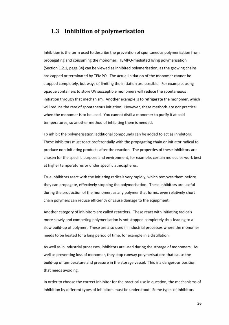
Scheme 15. The recombination of a radical initiator and TEMPO. ........................................ 39
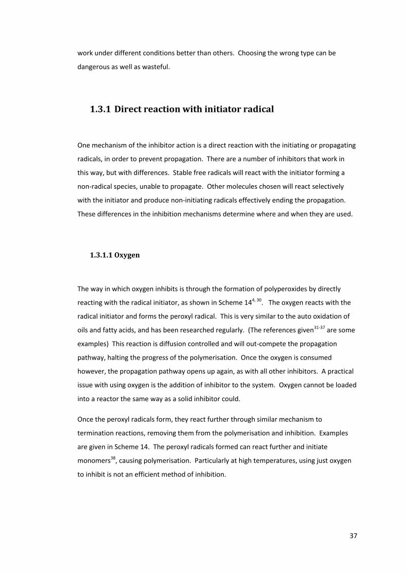
Scheme 16. The proposed reaction for benzyl radicals with nitrobenzene, proposed by
Jackson and Waters45, 46 ......................................................................................................... 40
Scheme 17. A variation of the mechanism in Scheme 1647-49 ................................................ 40
Scheme 18. The inhibition mechanism followed by benzoquinones50-54.............................. 41
Scheme 19. Electron donation by PTZ to an initiator radical ................................................ 42
Scheme 20. A possible route the PTZ radical cation can take after the initial inhibition. .... 42
Scheme 21. The mechanism for radical polymerisation inhibition. Top – Propagation.
Middle – Initiator reacting with oxygen. Bottom – Peroxyl radical abstracting hydrogen
from an inhibitor molecule, ArOH ......................................................................................... 43
Scheme 22. Schematic of the small scale, automated dilatometry setup, developed to
determine the onset of polymerisation after inhibition or retardation. ............................... 58
Scheme 23 A common polymerisation inhibitor (DNBP, left) with analogues investigated;
2,4-dinitrophenol (middle) and 2-nitrophenol (right) ........................................................... 72
Scheme 24. Demonstration of phenolic inhibition mechanism55, 85 ..................................... 76
16
Scheme 25. The resonance structures of a phenoxy radical ................................................ 77
Scheme 26. The resonance structures of 2-nitrophenol after phenolic hydrogen donation.
............................................................................................................................................... 78
Scheme 27. The proposed mechanism for the formation of a product isolated and
characterised by Bushby et al45. ............................................................................................ 88
Scheme 28. Formation of nitroso arene as proposed by Bartlett et al94, via a nitroxide
intermediate. ......................................................................................................................... 94
Scheme 29. Formation of nitroso arene proposed by Jackson and Waters46, via an
alkoxynitroxide intermediate. ................................................................................................ 95
Scheme 30. Formation of nitroxide from 2-nitrophenol, observed by EPR. ......................... 95
Scheme 31. Proposed formation of Unknown B following previous research by Jackson and
Waters46, and by Bushby et al45. ............................................................................................ 97
Scheme 32. Photolysis of chloroform99. .............................................................................. 117
Scheme 33. Photooxidation of chloroform97, 98. ................................................................. 117
Scheme 34. Mechanism of oxidation and formation of product observed by X-ray
crystallography. .................................................................................................................... 118
Scheme 35. Possible mechanism for the formation of Unknown B. .................................. 120
Scheme 36. Retro-synthetic analysis of compound A. ........................................................ 121
Scheme 37 Synthesis of compound D100 .............................................................................. 122
Scheme 38. Formation of Imine (Compound E) from compound D and 2-aminophenol ... 129
Scheme 39. Mechanism of the formation of unknown B from compound E. .................... 130
Scheme 40. Hydrogen abstraction from 2-aminophenol by an initiator radical. ............... 137
Scheme 41. Possible mechanism of an initiator radical adding to the imine, compound E.
............................................................................................................................................. 139
Scheme 42. Synthesis of compound F ................................................................................ 140
Scheme 43. Literature proposed mechanism for reaction of nitrosobenzene and styrene.
The m/z values are the [M+H]+ ions observed103. ................................................................ 146
Scheme 44. Possible route for the formation of products observed from the reaction
between 2-nitrosophenol and styrene ................................................................................ 151
Scheme 45. Demonstration of the exchange experiment .................................................. 153
Scheme 46. Formation of nitroxide from nitrone intermediate postulated based on work by
Kang et al103 .......................................................................................................................... 156
Scheme 47. The simplified reactions describing the formation of radical initiators, where M
is monomer, D is dimer and R the radical initiator. ............................................................. 158
17
Scheme 48. The initial reaction between 2-nitrophenol and an initiator radical. .............. 160
Scheme 49. The formation of Compound B . ...................................................................... 161
Scheme 50. Formation and degradation of charge transfer complex proposed by Yassin and
Rizk. ...................................................................................................................................... 164
Scheme 51. The proposed mechanism for the inhibition of polymerisation, at low amine
concentrations. .................................................................................................................... 165
Scheme 52. The initial step in the inhibition of polymerisation at high amine
concentrations. .................................................................................................................... 165
Scheme 53. The second step of the inhibition mechanism. ............................................... 165
Scheme 54 Chain transfer from ammonium ion to anion of the complex. ........................ 166
Scheme 55. Synthesis of chloranil radical anion potassium salt ......................................... 168
Scheme 56. Formation of mono-hydroxy substituted chloranil ......................................... 172
Scheme 57. Formation of radical anion dimers at peaks m/z 434.82 and m/z 452.78 ...... 172
Scheme 58. Formation of a radical anion trimer at peak m/z 624.76 ................................. 173
Scheme 59. Comproportionation / disproportionation between chloranil and tetrachloro
hydroquinone. ...................................................................................................................... 181
Scheme 60. Chemical exchange of 2,5 – di-tert-butyl semiquinone with 2,5 – di-tert-butyl
hydroquinone dianion. ......................................................................................................... 183
Scheme 61. The comproportionation / disproportionation equilibrium of 2,5 – di-tert-butyl
hydroquinone and 2,5 – di-tert-butylquinone ..................................................................... 186
Scheme 62. A possible mechanism for the formation of mono substituted product
observed in the reaction between the quinone and excess base. ...................................... 194
Scheme 63. The new comproportionation / disproportionation equilibrium set up in a
system of quinone and base ................................................................................................ 195
Scheme 64 Resonance structures for the radical anion showing the dissociation of the
sodium ion and equivalence of the aromatic hydrogens. ................................................... 196
Scheme 65 The slow ion exchange of the sodium ion, demonstrating the two different
proton environments ........................................................................................................... 197
18
List of tables
Table 1. Inhibition times of potential inhibitors, tested by heating 5 ml sample of the
inhibitor in styrene at 130°C.62 .............................................................................................. 52
Table 2. Table of change in volume after complete polymerisation for a number on
monomers75. Density measured at 25 °C unless denoted by a. ............................................ 55
Table 3. Results of GC/MS on styrene inhibited by 2-nitrophenol. ....................................... 93
Table 4. High field protons of unknown B. From 700 MHz data, performed in CDCl3. ....... 108
Table 5. Summary of proton signals for Unknown B and their couplings in COSY, HSQC and
HMBC NMR experiments. (700 MHz NMR experiments, performed in CDCl3.) ................. 114
Table 6. Summary of proton signals of compound D and their couplings in COSY, HSQC and
HMBC NMR experiments. (400 MHz, CDCl3)........................................................................ 125
Table 7 Structures of fragments formed in the MS / MS experiment on Unknown B or
Compound A ........................................................................................................................ 133
Table 8. Possible structures of products from the decomposition of chloranil radical anion
potassium salt in water. The MS peaks correspond to [M+H]+ ions of the proposed
structures. ............................................................................................................................ 171
Table 9. Equilibrium constants, enthalpy and entropy for the comproportionation /
disproportionation equilibrium in ethanol .......................................................................... 190
Table 10. Structures for possible products for the decomposition of quinone in base ...... 194
Table 11. Equilibrium constants, enthalpy and entropy for the comproportionation /
disproportionation equilibrium of 2,5 – di-tert-butyl hydroquinone and 2,5 – di-tert-
butylquinonein 2% ethanol / toluene .................................................................................. 200
Table 12. CHN results for chloranil radical anion potassium salt ....................................... 209
Table 13. Summary of carbon signals and their couplings in HSQC and HMBC NMR
experiments (700MHz, CDCl3) .............................................................................................. 220
Table 14. Summary of carbon signals of compound D and their couplings in COSY, TOCSY,
HSQC and HMBC NMR experiments. (400MHz, CDCl3) ....................................................... 226
Table 15. Crystal data and structure refinement for Unknown B........................................ 227
Table 16. Fractional Atomic Coordinates (×104) and Equivalent Isotropic Displacement
Parameters (Å2×10³) for vc1301. Ueq is defined as 1/3 of of the trace of the orthogonalised
UIJ tensor. ............................................................................................................................. 228
Table 17. Anisotropic Displacement Parameters (Å2×10³) for vc1301. The Anisotropic
displacement factor exponent takes the form: -2π2[h2a*2U11+...+2hka×b×U12] ................. 229

19
Table 18. Bond lengths for Unknown B as determined by X-ray crystallography ............... 230
Table 19. Bond Angles for Unknown B as determined by X-ray crystallography ................ 231
Table 20. Hydrogen Atom Coordinates (Å×104) and Isotropic Displacement Parameters
(Å2×10³) for vc1301. ............................................................................................................ 232

20
List of equations
Equation 1. Determination of energy levels of an electron in an applied magnetic field. ... 45
Equation 2. Determination of level occupancy using the Maxwell-Boltzmann distribution 46
Equation 3. Formula for the calculation of Double Bond Number, where C is the number of
carbons, H the number of hydrogens, X the number of halogens and N the number of
nitrogens .............................................................................................................................. 116
Equation 4. Rate of formation of initiator radicals, from the reaction between monomer
and dimer. ............................................................................................................................ 158
Equation 5. Rate of formation of the styrene dimer. ......................................................... 158
Equation 6. The disproportionation of semiquinone radical to quinone and hydroquinone
............................................................................................................................................. 166
Equation 7. The rate equation for the equilibrium ([SQ], [Q] and [HQ] are concentrations of
semiquinone, quinone and hydroquinone.) ........................................................................ 186
Equation 8. The relationship between initial starting concentrations and the concentration
of components once equilibrium is established. ................................................................. 186
Equation 9. Combination of Equation 7 and Equation 8..................................................... 187
Equation 10. The rate equation for the equilibrium expanded, then arranged in way that
can be solved, and the coefficients a, b and c used to solve the quadratic equation ......... 187
Equation 11. The Eyring equation ....................................................................................... 190
Equation 12. Relationship between pKa and Ka .................................................................. 190
Equation 13. Determination of the acid dissociation constant, Ka. .................................... 191
Equation 14. Relationship between starting concentration of the acid ([HA]0) and the
concentration of the acid and the conjugate base in the system. ...................................... 191
Equation 15. Combining Equation 13 and Equation 14 ...................................................... 191
Equation 16. Determination of pH ...................................................................................... 191
Equation 17. Method of converting the literature data to a form comparable to the work
above.................................................................................................................................... 192
Equation 18. The relationship between the concentrations of semiquinone, quinone and
hydroquinone ....................................................................................................................... 200
Equation 19. The equilibrium equation simplified to include concentrations of observable
species .................................................................................................................................. 200
Equation 20. The quadratic equation that can be solved, to determine the remaining
semiquinone concentration. ................................................................................................ 201
21
Acknowledgments
This thesis would not have been possible without the support, help, advice and distractions
from many people. I hope to express my thanks to as many as I can below.
I’d like to thanks my parents, Jane and Alastair, and my sister, Lorna, for their never ending
support before, during and after my time at university.
I would like to thank Victor for his patience, technical know-how and down to earth
support he gave me over the past 4 years. Thanks also to the VC Group over the years;
Kazim, Rob S, Chiara, Sindhu, Zhou, Rob T, Dave, Jamie, James and Warsi. I hope I helped
you as much you all helped me (probably not though). Thanks also to the people outside of
the VC madness; Kate, Chris, Natalie P, Danielle, Rob M, and even to the undergrads who I
have demonstrated over the years.
I would like to thank the people at Nufarm Ltd for their support; Peter, Colin, Angela, Andy,
Steve and Tony.
A huge thanks and hug has to go to Jennifer, whose help has kept me “sane” though this
endeavour. The Gilbert and Sullivan society and Pure Lindy also deserve praise for stopping
me from becoming a complete recluse, but especially thanks to Lauren, Chris, Vernia,
James G, James K, Morven, Sophie, Natalie S and Ella.
I dedicate this thesis to my grandfathers, Tom and Ted. The astute readers among you may
have noticed that I was named after both of them. Ted always asked how my time at
university going, but unfortunately passed away before it was complete. My other
granddad, Tom, passed away before I was even looking at universities. His nickname for
me was “Boots”, which I did not connect until recently with the name of another well-
known “chemist”. I would like to think that, wherever he may be, he is having the last
laugh now with a joke 27 years in the making.

22
That’s the sentimental part over. You’ve read your name (you know who you are) and
there is no need to read on any further. It’s just chemistry from this point on.
23
Authors declaration
The following was carried out by Thomas Edward Newby, under the supervision of Dr Victor
Chechik. This work has not previously been presented for an award at this, or any other,
University. All sources are acknowledged as References.
The NMR analysis of unknown Compound B and ketone compound D was performed with
the assistance of Dr Robert J Thatcher.
A number of DFT calculations were performed by Kate Horner.
24
1. Introduction
Polymers are an important material used throughout the world. The production of
monomers for plastics is therefore a diverse and grand scale operation. In 2010,
approximately 25 million tons of styrene were produced globally.1 Understanding the
production of these polymers, and how they are controlled, is vital to meet the world’s
demand.
1.1 Properties of a polymer
The properties of the polymer depend upon a number of factors. The most observable
property that relates directly to the structure and make-up of the polymer is the Glass
Transition Temperature, Tg2. This is given as the temperature when the Gibbs free energy is
above the energy needed for the polymer chains to move over each other when a force is
applied. Visibly, this results in the plastic going from hard and brittle to malleable and
rubber-like. The interactions between the chains affect this value greatly. For example,
the addition of hydrogen bonds between chains greatly increase the activation energy
needed for the chains to move over one another, and therefore the glass transition
temperature increases also.
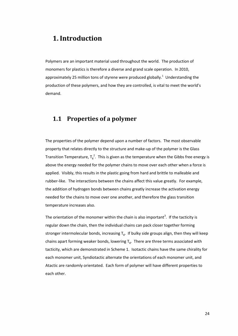
The orientation of the monomer within the chain is also important3. If the tacticity is
regular down the chain, then the individual chains can pack closer together forming
stronger intermolecular bonds, increasing Tg. If bulky side groups align, then they will keep
chains apart forming weaker bonds, lowering Tg. There are three terms associated with
tacticity, which are demonstrated in Scheme 1. Isotactic chains have the same chirality for
each monomer unit, Syndiotactic alternate the orientations of each monomer unit, and
Atactic are randomly orientated. Each form of polymer will have different properties to
each other.
25
n
n
n
Isotactic
Syndiotactic
Atactic
Scheme 1 Demonstration of tacticity of polymers3
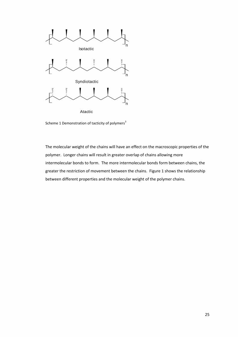
The molecular weight of the chains will have an effect on the macroscopic properties of the
polymer. Longer chains will result in greater overlap of chains allowing more
intermolecular bonds to form. The more intermolecular bonds form between chains, the
greater the restriction of movement between the chains. Figure 1 shows the relationship
between different properties and the molecular weight of the polymer chains.
26
Figure 1. Relationship between chain length of a polymer and its properties; viscosity, tensile and
impact strength
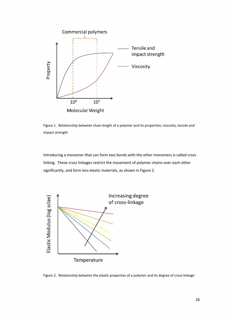
Introducing a monomer that can form two bonds with the other monomers is called cross
linking. These cross linkages restrict the movement of polymer chains over each other
significantly, and form less elastic materials, as shown in Figure 2.
Figure 2. Relationship between the elastic properties of a polymer and its degree of cross-linkage
27
Controlling the chemical reactions that form the polymer chains is vital to making polymer
materials that fit specific physical and mechanical properties.
1.2 Radical polymerisation
Radical polymerisation describes the mechanism of polymerisation where the propagation
species is a radical. Compared to similar cationic and anionic polymerisations, radical
polymerisation is less discriminating in the propagating reaction, leading to a greater
number of possible propagation and termination routes4.
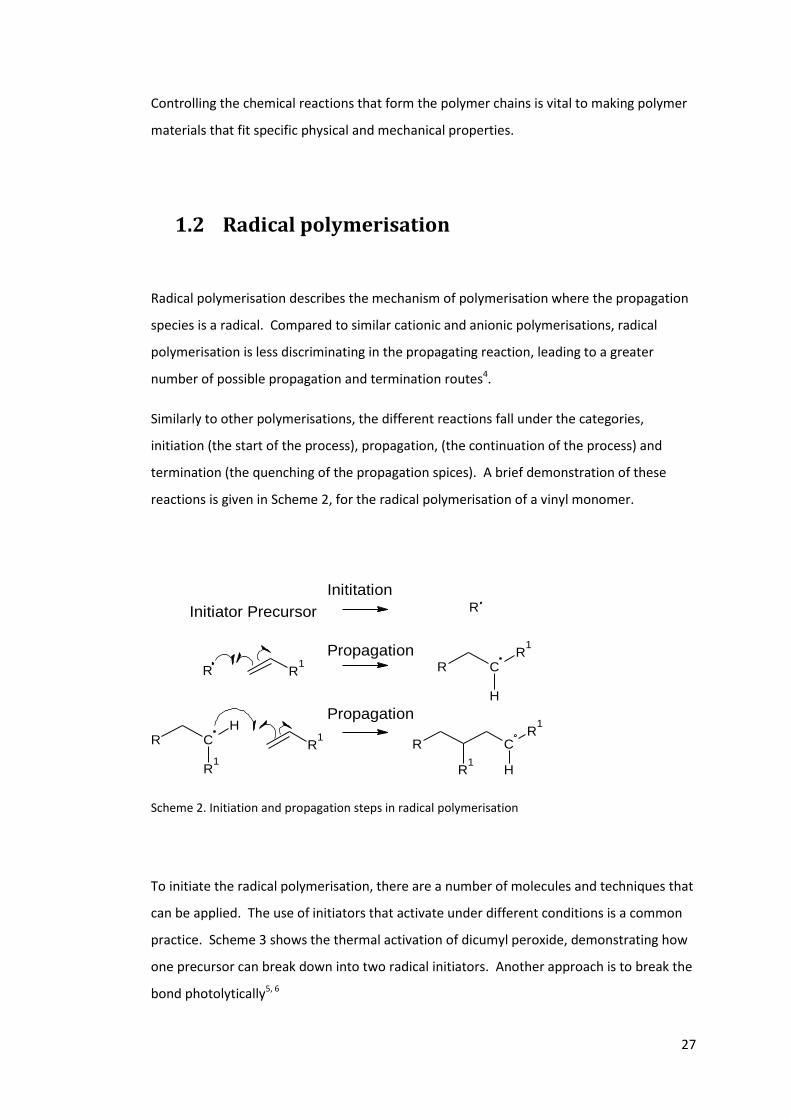
Similarly to other polymerisations, the different reactions fall under the categories,
initiation (the start of the process), propagation, (the continuation of the process) and
termination (the quenching of the propagation spices). A brief demonstration of these
reactions is given in Scheme 2, for the radical polymerisation of a vinyl monomer.
R
R R1 R C
R1
H
R C
R1
H
R1
R C
R1
R1
H
Initiator Precursor
Inititation
Propagation
Propagation
Scheme 2. Initiation and propagation steps in radical polymerisation
To initiate the radical polymerisation, there are a number of molecules and techniques that
can be applied. The use of initiators that activate under different conditions is a common
practice. Scheme 3 shows the thermal activation of dicumyl peroxide, demonstrating how
one precursor can break down into two radical initiators. Another approach is to break the
bond photolytically5, 6
28
OO
O2
Scheme 3 Thermal activation of dicumyl peroxide initiator
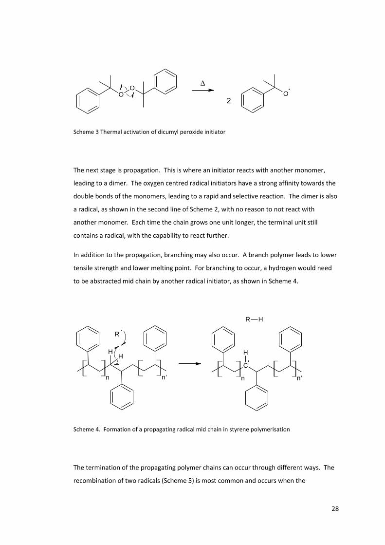
The next stage is propagation. This is where an initiator reacts with another monomer,
leading to a dimer. The oxygen centred radical initiators have a strong affinity towards the
double bonds of the monomers, leading to a rapid and selective reaction. The dimer is also
a radical, as shown in the second line of Scheme 2, with no reason to not react with
another monomer. Each time the chain grows one unit longer, the terminal unit still
contains a radical, with the capability to react further.
In addition to the propagation, branching may also occur. A branch polymer leads to lower
tensile strength and lower melting point. For branching to occur, a hydrogen would need
to be abstracted mid chain by another radical initiator, as shown in Scheme 4.
HH
n n'
R
C
H
n n'
R H
Scheme 4. Formation of a propagating radical mid chain in styrene polymerisation
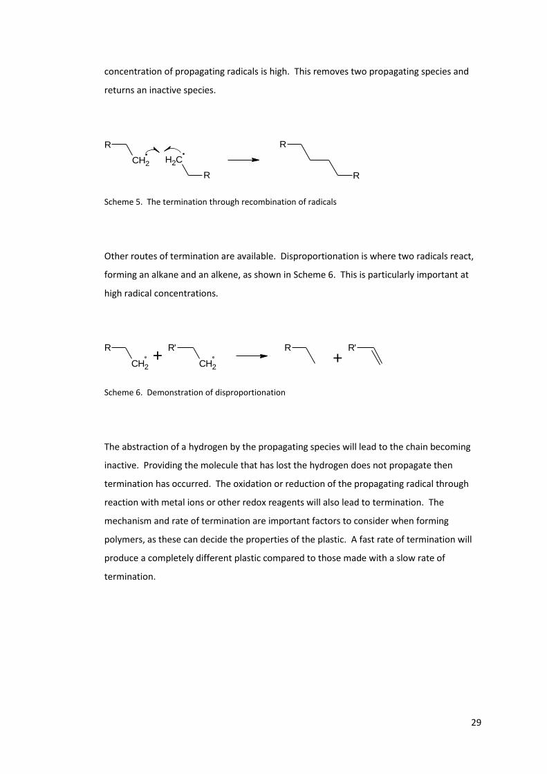
The termination of the propagating polymer chains can occur through different ways. The
recombination of two radicals (Scheme 5) is most common and occurs when the
29
concentration of propagating radicals is high. This removes two propagating species and
returns an inactive species.
R
CH2
R
CH2
R
R
Scheme 5. The termination through recombination of radicals
Other routes of termination are available. Disproportionation is where two radicals react,
forming an alkane and an alkene, as shown in Scheme 6. This is particularly important at
high radical concentrations.
R
CH2
R'
CH2+
R R'
+
Scheme 6. Demonstration of disproportionation
The abstraction of a hydrogen by the propagating species will lead to the chain becoming
inactive. Providing the molecule that has lost the hydrogen does not propagate then
termination has occurred. The oxidation or reduction of the propagating radical through
reaction with metal ions or other redox reagents will also lead to termination. The
mechanism and rate of termination are important factors to consider when forming
polymers, as these can decide the properties of the plastic. A fast rate of termination will
produce a completely different plastic compared to those made with a slow rate of
termination.
30
1.2.1 Spontaneous polymerisation
The use of initiator molecules is not the only way to start polymerisation. All monomers
will polymerise in one way or another when stored prior to use or when heated7, 8.
Spontaneous polymerisation produces polymers that have very little practical use, as well
as consuming monomer9. Another factor to include is the heat of polymerisation, as an
unchecked reaction will cause heat to build up in a container, as the polymerisation
reaction continues.
The mechanism of this spontaneous reaction varies between different types of monomer.
Also, there are cases of what appears to be spontaneous polymerisation, but the observed
polymerisation is actually due to other mechanisms. UV radiation can cause the formation
of initiators. Most monomers will react with oxygen, some forming hydroperoxides that
act as initiators. Monomers can also contain other impurities such as metals which could
lead to redox initiation. Combining these factors, apparently spontaneous initiation could
occur without the monomer reacting with itself.
However apart from these reactions, there are mechanisms for genuine self-initiation
which are discussed in this section.
1.2.1.1 Bi-radical mechanism
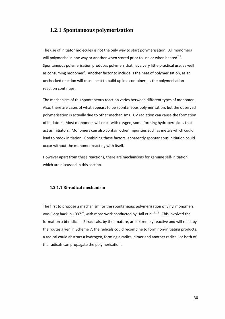
The first to propose a mechanism for the spontaneous polymerisation of vinyl monomers
was Flory back in 193710, with more work conducted by Hall et al11, 12. This involved the
formation a bi-radical. Bi-radicals, by their nature, are extremely reactive and will react by
the routes given in Scheme 7; the radicals could recombine to form non-initiating products;
a radical could abstract a hydrogen, forming a radical dimer and another radical; or both of
the radicals can propagate the polymerisation.
31
R
2
CH
CH
R
R
R
R
Propagation
R CH
R
Non-initiating product
Scheme 7. The initiation of vinyl monomers proposed by Hall11, 12
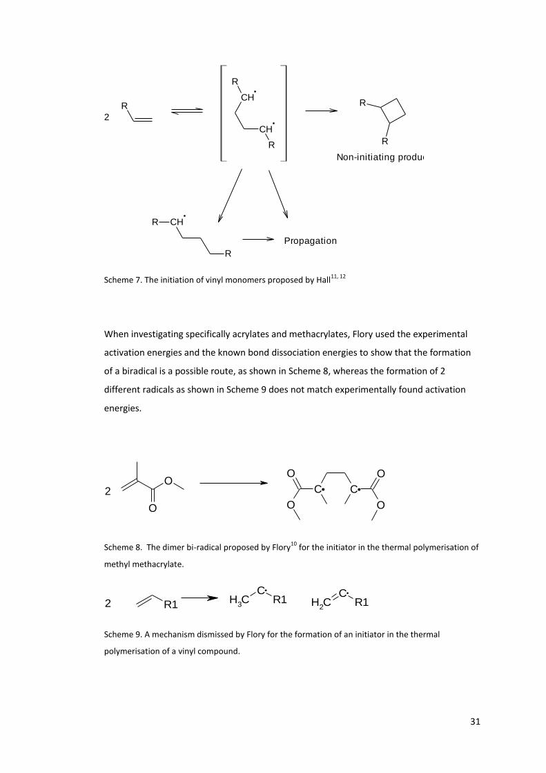
When investigating specifically acrylates and methacrylates, Flory used the experimental
activation energies and the known bond dissociation energies to show that the formation
of a biradical is a possible route, as shown in Scheme 8, whereas the formation of 2
different radicals as shown in Scheme 9 does not match experimentally found activation
energies.
O
OC C
OO
OO
2
Scheme 8. The dimer bi-radical proposed by Flory10
for the initiator in the thermal polymerisation of
methyl methacrylate.
R1 CH3
C
R1 CH2
C
R12
Scheme 9. A mechanism dismissed by Flory for the formation of an initiator in the thermal
polymerisation of a vinyl compound.
32
The biradical mechanism was also suggested for the formation of some of the dimers
observed by Lignau et al13, as discussed earlier. Figure 3 shows the dimers cCB and tCB,
which could form from the biradical.
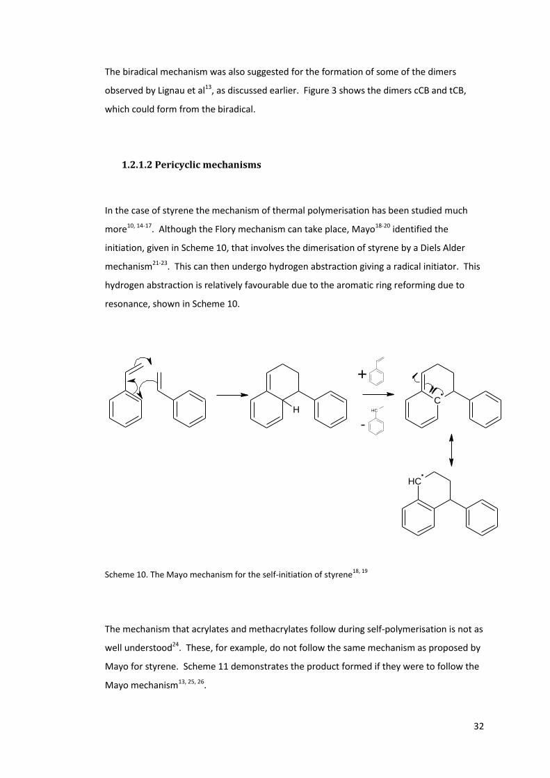
1.2.1.2 Pericyclic mechanisms
In the case of styrene the mechanism of thermal polymerisation has been studied much
more10, 14-17. Although the Flory mechanism can take place, Mayo18-20 identified the
initiation, given in Scheme 10, that involves the dimerisation of styrene by a Diels Alder
mechanism21-23. This can then undergo hydrogen abstraction giving a radical initiator. This
hydrogen abstraction is relatively favourable due to the aromatic ring reforming due to
resonance, shown in Scheme 10.
HC
CH
CH
+
Scheme 10. The Mayo mechanism for the self-initiation of styrene18, 19
The mechanism that acrylates and methacrylates follow during self-polymerisation is not as
well understood24. These, for example, do not follow the same mechanism as proposed by
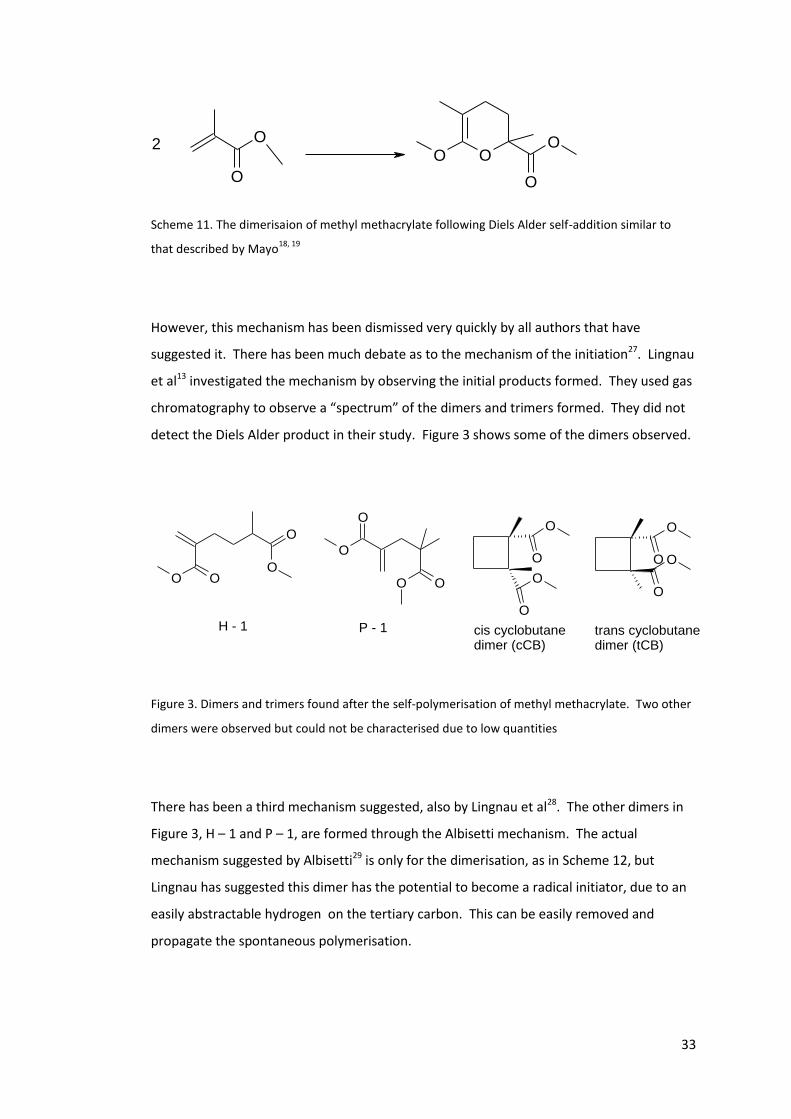
Mayo for styrene. Scheme 11 demonstrates the product formed if they were to follow the
Mayo mechanism13, 25, 26.
33
O
OOO
O
O2
Scheme 11. The dimerisaion of methyl methacrylate following Diels Alder self-addition similar to
that described by Mayo18, 19
However, this mechanism has been dismissed very quickly by all authors that have
suggested it. There has been much debate as to the mechanism of the initiation27. Lingnau
et al13 investigated the mechanism by observing the initial products formed. They used gas
chromatography to observe a “spectrum” of the dimers and trimers formed. They did not
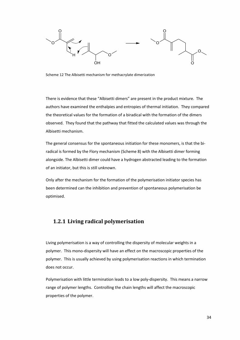
detect the Diels Alder product in their study. Figure 3 shows some of the dimers observed.
O
O O
OO
O
O
O
O OO
O
O O
O
O
H - 1 P - 1 cis cyclobutanedimer (cCB)
trans cyclobutanedimer (tCB)
Figure 3. Dimers and trimers found after the self-polymerisation of methyl methacrylate. Two other
dimers were observed but could not be characterised due to low quantities
There has been a third mechanism suggested, also by Lingnau et al28. The other dimers in
Figure 3, H – 1 and P – 1, are formed through the Albisetti mechanism. The actual
mechanism suggested by Albisetti29 is only for the dimerisation, as in Scheme 12, but
Lingnau has suggested this dimer has the potential to become a radical initiator, due to an
easily abstractable hydrogen on the tertiary carbon. This can be easily removed and
propagate the spontaneous polymerisation.
34
O
O
H
OH
O
O
O
O
O
Scheme 12 The Albisetti mechanism for methacrylate dimerization
There is evidence that these “Albisetti dimers” are present in the product mixture. The
authors have examined the enthalpies and entropies of thermal initiation. They compared
the theoretical values for the formation of a biradical with the formation of the dimers
observed. They found that the pathway that fitted the calculated values was through the
Albisetti mechanism.
The general consensus for the spontaneous initiation for these monomers, is that the bi-
radical is formed by the Flory mechanism (Scheme 8) with the Albisetti dimer forming
alongside. The Albisetti dimer could have a hydrogen abstracted leading to the formation
of an initiator, but this is still unknown.
Only after the mechanism for the formation of the polymerisation initiator species has
been determined can the inhibition and prevention of spontaneous polymerisation be
optimised.
1.2.1 Living radical polymerisation
Living polymerisation is a way of controlling the dispersity of molecular weights in a
polymer. This mono-dispersity will have an effect on the macroscopic properties of the
polymer. This is usually achieved by using polymerisation reactions in which termination
does not occur.
Polymerisation with little termination leads to a low poly-dispersity. This means a narrow
range of polymer lengths. Controlling the chain lengths will affect the macroscopic
properties of the polymer.
35
Living polymerisations have the ability to continue until all of the monomer is consumed.
Then, they have the ability to continue with the addition of more monomer, either the
same type or a different monomer. This is one method of producing block co-polymers.
In radical living polymerisation it is difficult to remove the termination pathways, due to
the nature of radicals themselves. Therefore, a different approach is used for controlling
the polymerisation, such as making the termination step reversible.
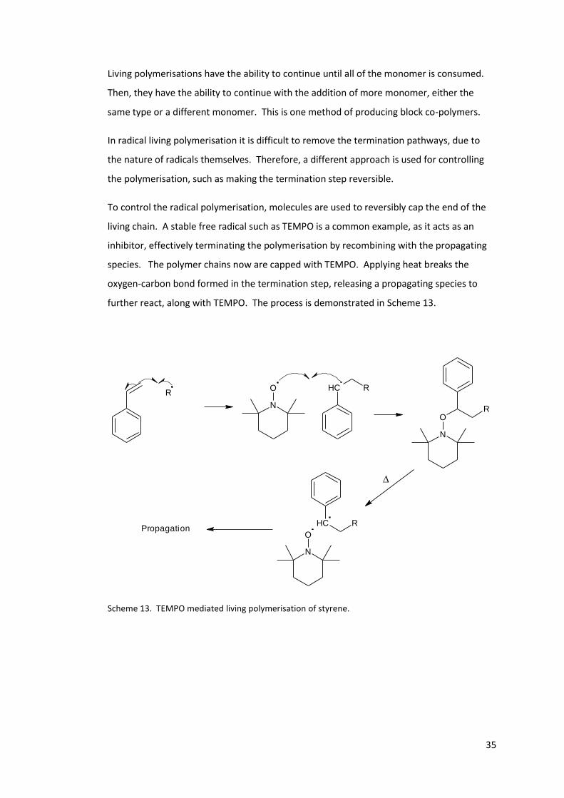
To control the radical polymerisation, molecules are used to reversibly cap the end of the
living chain. A stable free radical such as TEMPO is a common example, as it acts as an
inhibitor, effectively terminating the polymerisation by recombining with the propagating
species. The polymer chains now are capped with TEMPO. Applying heat breaks the
oxygen-carbon bond formed in the termination step, releasing a propagating species to
further react, along with TEMPO. The process is demonstrated in Scheme 13.
N
O CH R
N
OR
N
O
CH R
Propagation
R
Scheme 13. TEMPO mediated living polymerisation of styrene.
36
1.3 Inhibition of polymerisation
Inhibition is the term used to describe the prevention of spontaneous polymerisation from
propagating and consuming the monomer. TEMPO-mediated living polymerisation
(Section 1.2.1, page 34) can be viewed as inhibited polymerisation, as the growing chains
are capped or terminated by TEMPO. The actual initiation of the monomer cannot be
stopped completely, but ways of limiting the initiation are possible. For example, using
opaque containers to store UV susceptible monomers will reduce the spontaneous
initiation through that mechanism. Another example is to refrigerate the monomer, which
will reduce the rate of spontaneous initiation. However, these methods are not practical
when the monomer is to be used. You cannot distil a monomer to purify it at cold
temperatures, so another method of inhibiting them is needed.
To inhibit the polymerisation, additional compounds can be added to act as inhibitors.
These inhibitors must react preferentially with the propagating chain or initiator radical to
produce non-initiating products after the reaction. The properties of these inhibitors are
chosen for the specific purpose and environment, for example, certain molecules work best
at higher temperatures or under specific atmospheres.
True inhibitors react with the initiating radicals very rapidly, which removes them before
they can propagate, effectively stopping the polymerisation. These inhibitors are useful
during the production of the monomer, as any polymer that forms, even relatively short
chain polymers can reduce efficiency or cause damage to the equipment.
Another category of inhibitors are called retarders. These react with initiating radicals
more slowly and competing polymerisation is not stopped completely thus leading to a
slow build-up of polymer. These are also used in industrial processes where the monomer
needs to be heated for a long period of time, for example in a distillation.
As well as in industrial processes, inhibitors are used during the storage of monomers. As
well as preventing loss of monomer, they stop runway polymerisations that cause the
build-up of temperature and pressure in the storage vessel. This is a dangerous position
that needs avoiding.
In order to choose the correct inhibitor for the practical use in question, the mechanisms of
inhibition by different types of inhibitors must be understood. Some types of inhibitors
37
work under different conditions better than others. Choosing the wrong type can be
dangerous as well as wasteful.
1.3.1 Direct reaction with initiator radical
One mechanism of the inhibitor action is a direct reaction with the initiating or propagating
radicals, in order to prevent propagation. There are a number of inhibitors that work in
this way, but with differences. Stable free radicals will react with the initiator forming a
non-radical species, unable to propagate. Other molecules chosen will react selectively
with the initiator and produce non-initiating radicals effectively ending the propagation.
These differences in the inhibition mechanisms determine where and when they are used.
1.3.1.1 Oxygen
The way in which oxygen inhibits is through the formation of polyperoxides by directly
reacting with the radical initiator, as shown in Scheme 144, 30. The oxygen reacts with the
radical initiator and forms the peroxyl radical. This is very similar to the auto oxidation of
oils and fatty acids, and has been researched regularly. (The references given31-37 are some
examples) This reaction is diffusion controlled and will out-compete the propagation
pathway, halting the progress of the polymerisation. Once the oxygen is consumed
however, the propagation pathway opens up again, as with all other inhibitors. A practical
issue with using oxygen is the addition of inhibitor to the system. Oxygen cannot be loaded
into a reactor the same way as a solid inhibitor could.
Once the peroxyl radicals form, they react further through similar mechanism to
termination reactions, removing them from the polymerisation and inhibition. Examples
are given in Scheme 14. The peroxyl radicals formed can react further and initiate
monomers38, causing polymerisation. Particularly at high temperatures, using just oxygen
to inhibit is not an efficient method of inhibition.

38
RO
OR
OO
RO
O2 R
OO
R + O2
RO
O RO
OR
R
RO
OH R
RO
OH
R+
Scheme 14. Formation of peroxyl radical, polyperoxide and hydroperoxide.30
1.3.1.2 Stable radicals
The recombination of radicals is an important termination route in any polymerisation. As
the concentration of radicals increases, the rate of recombination increases as well. The
use of stable free radicals as inhibitors comes from this logic39-41.
A common inhibitor used is 2,2,6,6-tetramethyl-1-piperidinyloxy (TEMPO) and similar
derivatives42-44. By adding these stable radicals to the monomer sample, the
polymerisation is inhibited as the propagating radical and a TEMPO radical would
recombine, effectively increasing the rate of termination. The rate constant of styrene
propagation42 is 2.2 x 10³ M-1 s-1, whereas the rate of reaction between TEMPO and a
styrene initiator42 is 8 x 10⁸ M-1 s-1. This means TEMPO will out-compete styrene
polymerisation propagation even at low concentration.
These inhibitors directly react with the initiator to remove it from the propagation, as in
Scheme 15, rather than relying on oxygen to react first.
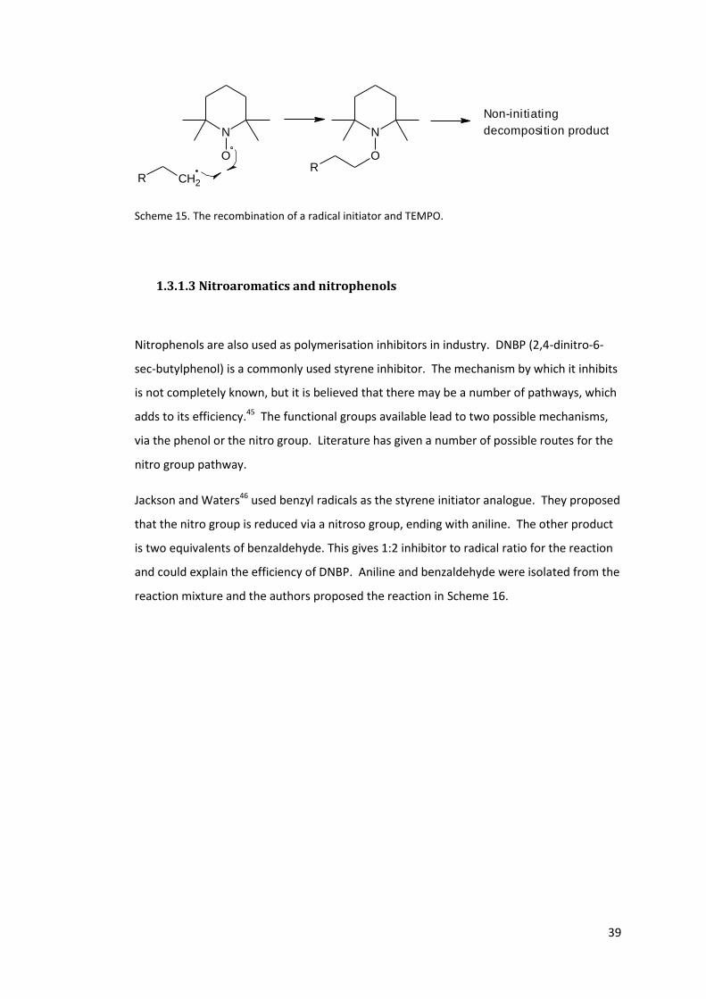
39
N
O
R CH2
N
OR
Non-initiating
decomposition products
Scheme 15. The recombination of a radical initiator and TEMPO.
1.3.1.3 Nitroaromatics and nitrophenols
Nitrophenols are also used as polymerisation inhibitors in industry. DNBP (2,4-dinitro-6-
sec-butylphenol) is a commonly used styrene inhibitor. The mechanism by which it inhibits
is not completely known, but it is believed that there may be a number of pathways, which
adds to its efficiency.45 The functional groups available lead to two possible mechanisms,
via the phenol or the nitro group. Literature has given a number of possible routes for the
nitro group pathway.
Jackson and Waters46 used benzyl radicals as the styrene initiator analogue. They proposed
that the nitro group is reduced via a nitroso group, ending with aniline. The other product
is two equivalents of benzaldehyde. This gives 1:2 inhibitor to radical ratio for the reaction
and could explain the efficiency of DNBP. Aniline and benzaldehyde were isolated from the
reaction mixture and the authors proposed the reaction in Scheme 16.
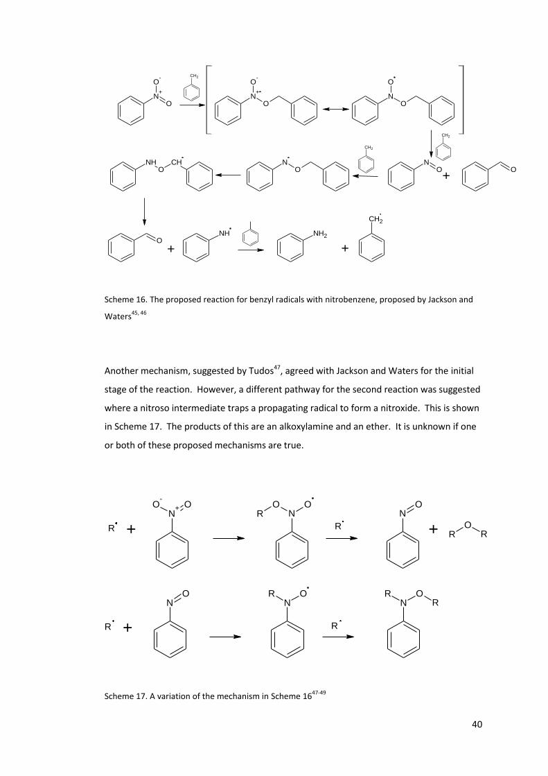
40
N+
O
O-
N+
O
O-CH2
NO
O
O+
NO
CH2
NO
NHO
CH
O
+
NH
CH2
+
NH2
CH2
Scheme 16. The proposed reaction for benzyl radicals with nitrobenzene, proposed by Jackson and
Waters45, 46
Another mechanism, suggested by Tudos47, agreed with Jackson and Waters for the initial
stage of the reaction. However, a different pathway for the second reaction was suggested
where a nitroso intermediate traps a propagating radical to form a nitroxide. This is shown
in Scheme 17. The products of this are an alkoxylamine and an ether. It is unknown if one
or both of these proposed mechanisms are true.
N+ OO
-
R +N
OOR
R
NO
RO
R+
NO
R +
NOR
NOR
R
R
Scheme 17. A variation of the mechanism in Scheme 1647-49
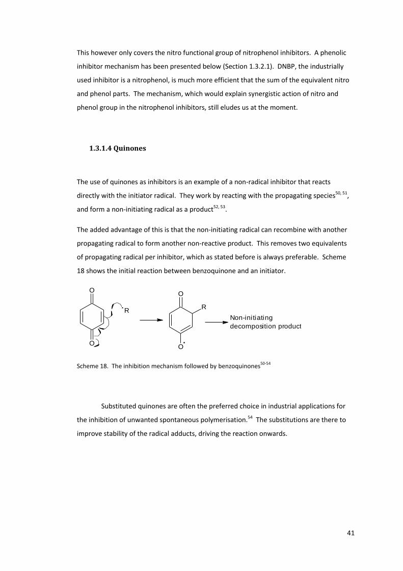
41
This however only covers the nitro functional group of nitrophenol inhibitors. A phenolic
inhibitor mechanism has been presented below (Section 1.3.2.1). DNBP, the industrially
used inhibitor is a nitrophenol, is much more efficient that the sum of the equivalent nitro
and phenol parts. The mechanism, which would explain synergistic action of nitro and
phenol group in the nitrophenol inhibitors, still eludes us at the moment.
1.3.1.4 Quinones
The use of quinones as inhibitors is an example of a non-radical inhibitor that reacts
directly with the initiator radical. They work by reacting with the propagating species50, 51,
and form a non-initiating radical as a product52, 53.
The added advantage of this is that the non-initiating radical can recombine with another
propagating radical to form another non-reactive product. This removes two equivalents
of propagating radical per inhibitor, which as stated before is always preferable. Scheme
18 shows the initial reaction between benzoquinone and an initiator.
O
O
R
O
O
R
Non-initiating
decomposition products
Scheme 18. The inhibition mechanism followed by benzoquinones50-54
Substituted quinones are often the preferred choice in industrial applications for
the inhibition of unwanted spontaneous polymerisation.54 The substitutions are there to
improve stability of the radical adducts, driving the reaction onwards.
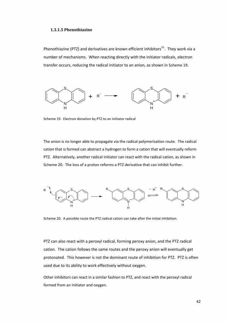
42
1.3.1.5 Phenothiazine
Phenothiazine (PTZ) and derivatives are known efficient inhibitors55. They work via a
number of mechanisms. When reacting directly with the initiator radicals, electron
transfer occurs, reducing the radical initiator to an anion, as shown in Scheme 19.
S
NH
S
NH
+
R R+ +
Scheme 19. Electron donation by PTZ to an initiator radical
The anion is no longer able to propagate via the radical polymerisation route. The radical
cation that is formed can abstract a hydrogen to form a cation that will eventually reform
PTZ. Alternatively, another radical initiator can react with the radical cation, as shown in
Scheme 20. The loss of a proton reforms a PTZ derivative that can inhibit further.
S
NH
+
R S
N+
R
H
S
NH
RH+
Scheme 20. A possible route the PTZ radical cation can take after the initial inhibition.
PTZ can also react with a peroxyl radical, forming peroxy anion, and the PTZ radical
cation. The cation follows the same routes and the peroxy anion will eventually get
protonated. This however is not the dominant route of inhibition for PTZ. PTZ is often
used due to its ability to work effectively without oxygen.
Other inhibitors can react in a similar fashion to PTZ, and react with the peroxyl radical
formed from an initiator and oxygen.
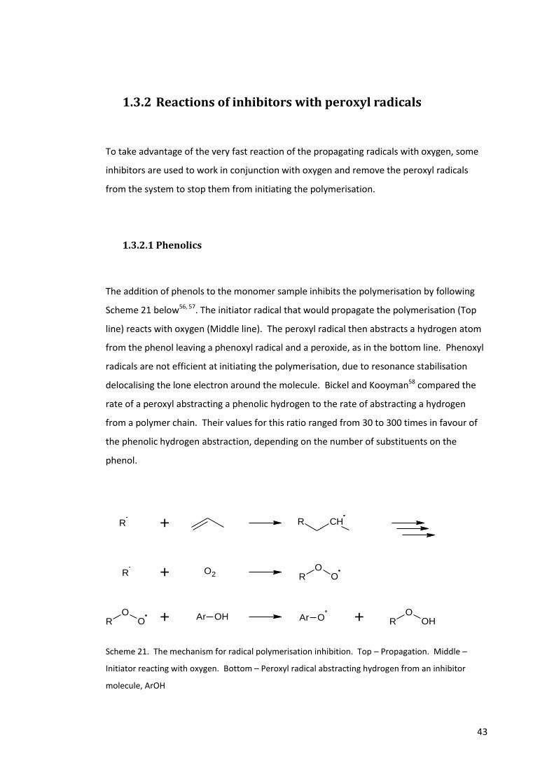
43
1.3.2 Reactions of inhibitors with peroxyl radicals
To take advantage of the very fast reaction of the propagating radicals with oxygen, some
inhibitors are used to work in conjunction with oxygen and remove the peroxyl radicals
from the system to stop them from initiating the polymerisation.
1.3.2.1 Phenolics
The addition of phenols to the monomer sample inhibits the polymerisation by following
Scheme 21 below56, 57. The initiator radical that would propagate the polymerisation (Top
line) reacts with oxygen (Middle line). The peroxyl radical then abstracts a hydrogen atom
from the phenol leaving a phenoxyl radical and a peroxide, as in the bottom line. Phenoxyl
radicals are not efficient at initiating the polymerisation, due to resonance stabilisation
delocalising the lone electron around the molecule. Bickel and Kooyman58 compared the
rate of a peroxyl abstracting a phenolic hydrogen to the rate of abstracting a hydrogen
from a polymer chain. Their values for this ratio ranged from 30 to 300 times in favour of
the phenolic hydrogen abstraction, depending on the number of substituents on the
phenol.
CHR+
+
+
R
R RO
O
RO
OAr OH Ar O R
OOH+
O2
Scheme 21. The mechanism for radical polymerisation inhibition. Top – Propagation. Middle –
Initiator reacting with oxygen. Bottom – Peroxyl radical abstracting hydrogen from an inhibitor
molecule, ArOH
44
The phenoxyl radical that forms can indeed react with another radical initiator, through
recombination. This makes the inhibitor more efficient; one molecule of inhibitor removes
two initiators.
As demonstrated above, analytical techniques, such as NMR and mass spectrometry, are
vital in determining the mechanism of inhibition. This study is to determine possible
pathways for old and new inhibitors. A technique that is less common, but could be of
great use is Electron Paramagnetic Resonance. This technique can observe radicals
directly, so could be used to monitor the rate of reaction with stable free radicals (e.g.
TEMPO), or could be used to identify a radical intermediate. Also it can be used to monitor
other variables in the reaction system, such as oxygen concentration.
1.4 Electron paramagnetic resonance
As previously stated, analytical techniques such as NMR, MS and GC are used to work
backwards to determine the reaction mechanism of inhibitors. However, observing the
reactive species may not be possible in radical polymerisation due to their high reactivity.
Electron Paramagnetic Resonance may be able to observe stable radical species in situ and
shed more light on the intermediates of the inhibition reaction.
Electron Paramagnetic Resonance (EPR, also known as Electron Spin Resonance, ESR) is
among the most direct methods of radical characterisation59, 60. This method is similar to
NMR, with the general difference being that NMR observes the transitions of the nuclear
spin, whereas EPR looks at electron spin transitions. EPR spectroscopy therefore can only
study systems with unpaired electrons and is particularly useful for characterisation of
paramagnetic species.
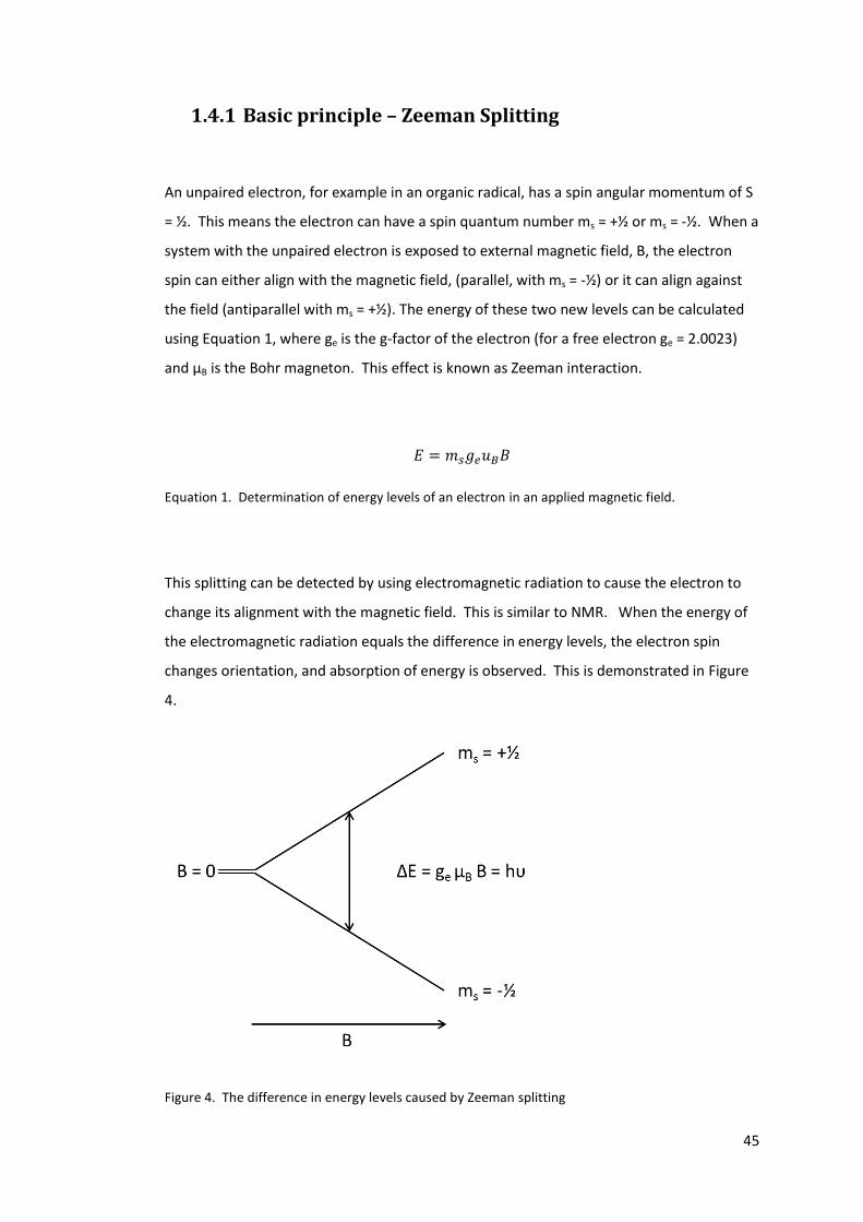
45
1.4.1 Basic principle – Zeeman Splitting
An unpaired electron, for example in an organic radical, has a spin angular momentum of S
= ½. This means the electron can have a spin quantum number ms = +½ or ms = -½. When a
system with the unpaired electron is exposed to external magnetic field, B, the electron
spin can either align with the magnetic field, (parallel, with ms = -½) or it can align against
the field (antiparallel with ms = +½). The energy of these two new levels can be calculated
using Equation 1, where ge is the g-factor of the electron (for a free electron ge = 2.0023)
and μB is the Bohr magneton. This effect is known as Zeeman interaction.
𝐸 = 𝑚𝑠𝑔𝑒𝑢𝐵𝐵
Equation 1. Determination of energy levels of an electron in an applied magnetic field.
This splitting can be detected by using electromagnetic radiation to cause the electron to
change its alignment with the magnetic field. This is similar to NMR. When the energy of
the electromagnetic radiation equals the difference in energy levels, the electron spin
changes orientation, and absorption of energy is observed. This is demonstrated in Figure
4.
Figure 4. The difference in energy levels caused by Zeeman splitting
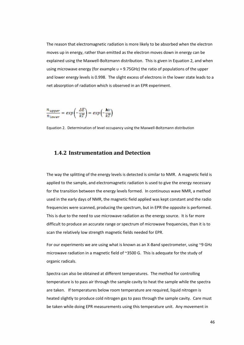
46
The reason that electromagnetic radiation is more likely to be absorbed when the electron
moves up in energy, rather than emitted as the electron moves down in energy can be
explained using the Maxwell-Boltzmann distribution. This is given in Equation 2, and when
using microwave energy (for example υ = 9.75GHz) the ratio of populations of the upper
and lower energy levels is 0.998. The slight excess of electrons in the lower state leads to a
net absorption of radiation which is observed in an EPR experiment.
Equation 2. Determination of level occupancy using the Maxwell-Boltzmann distribution
1.4.2 Instrumentation and Detection
The way the splitting of the energy levels is detected is similar to NMR. A magnetic field is
applied to the sample, and electromagnetic radiation is used to give the energy necessary
for the transition between the energy levels formed. In continuous wave NMR, a method
used in the early days of NMR, the magnetic field applied was kept constant and the radio
frequencies were scanned, producing the spectrum, but in EPR the opposite is performed.
This is due to the need to use microwave radiation as the energy source. It is far more
difficult to produce an accurate range or spectrum of microwave frequencies, than it is to
scan the relatively low strength magnetic fields needed for EPR.
For our experiments we are using what is known as an X-Band spectrometer, using ~9 GHz
microwave radiation in a magnetic field of ~3500 G. This is adequate for the study of
organic radicals.
Spectra can also be obtained at different temperatures. The method for controlling
temperature is to pass air through the sample cavity to heat the sample while the spectra
are taken. If temperatures below room temperature are required, liquid nitrogen is
heated slightly to produce cold nitrogen gas to pass through the sample cavity. Care must
be taken while doing EPR measurements using this temperature unit. Any movement in
47
the sample caused by the flow of gas will affect the intensity of the signal observed. Also
water condensing in the sample cavity will affect the spectra observed. These can be easily
overcome by using a stabilising bracket and passing dry nitrogen through the cavity as well
as the heated air or cooled nitrogen.
1.4.2.1 Noise reduction and sensitivity
To improve the sensitivity of the method, a number of techniques are employed. First, the
magnetic field is modulated, normally at frequencies around 100 kHz. At the detector, the
phase-sensitive detection of the signal oscillations that matches the modulation of the
magnetic field results in removing some of the background noise. This is relatively easy to
do as the magnetic field is weak compared to NMR.
A final method of improving the signal to noise ratio is to take the average of a number of
scans. This will remove more of the background noise. However, this is not applicable to
short lived radicals. For example, any decrease in signal from the species being observed in
the second scan will decrease the signal of the first scan when averaged. This method is
best applied for low concentrations of stable radicals or a steady state concentration of
radicals.
From the above, obtaining an informative and complete spectra relies upon a number of
parameters. However a large amount of information can be obtained from this technique
when decent spectra are obtained.
1.4.3 Analysis and interpretation of spectra
Determining if the sample contains an unpaired electron or not is not the limit of this
technique! A lot more information can be obtained from the interpretation of the spectra.
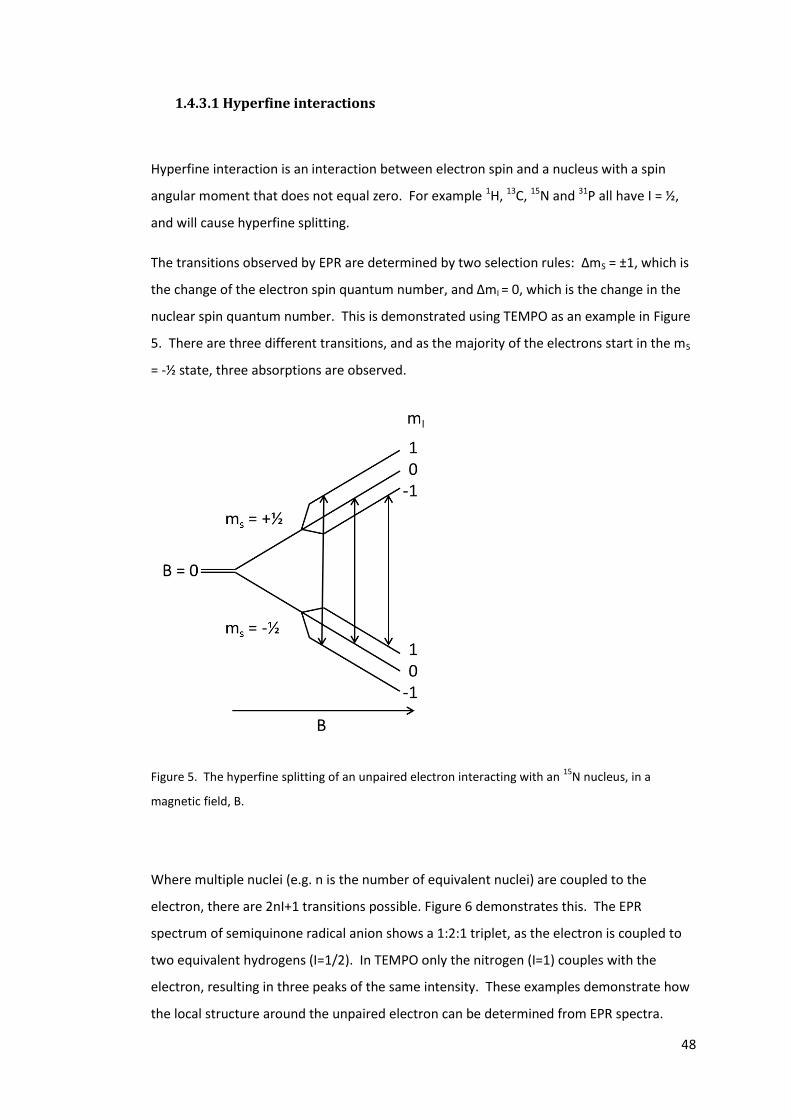
48
1.4.3.1 Hyperfine interactions
Hyperfine interaction is an interaction between electron spin and a nucleus with a spin
angular moment that does not equal zero. For example 1H, 13C, 15N and 31P all have I = ½,
and will cause hyperfine splitting.
The transitions observed by EPR are determined by two selection rules: ΔmS = ±1, which is
the change of the electron spin quantum number, and ΔmI = 0, which is the change in the
nuclear spin quantum number. This is demonstrated using TEMPO as an example in Figure
5. There are three different transitions, and as the majority of the electrons start in the mS
= -½ state, three absorptions are observed.
Figure 5. The hyperfine splitting of an unpaired electron interacting with an 15
N nucleus, in a
magnetic field, B.
Where multiple nuclei (e.g. n is the number of equivalent nuclei) are coupled to the
electron, there are 2nI+1 transitions possible. Figure 6 demonstrates this. The EPR
spectrum of semiquinone radical anion shows a 1:2:1 triplet, as the electron is coupled to
two equivalent hydrogens (I=1/2). In TEMPO only the nitrogen (I=1) couples with the
electron, resulting in three peaks of the same intensity. These examples demonstrate how
the local structure around the unpaired electron can be determined from EPR spectra.
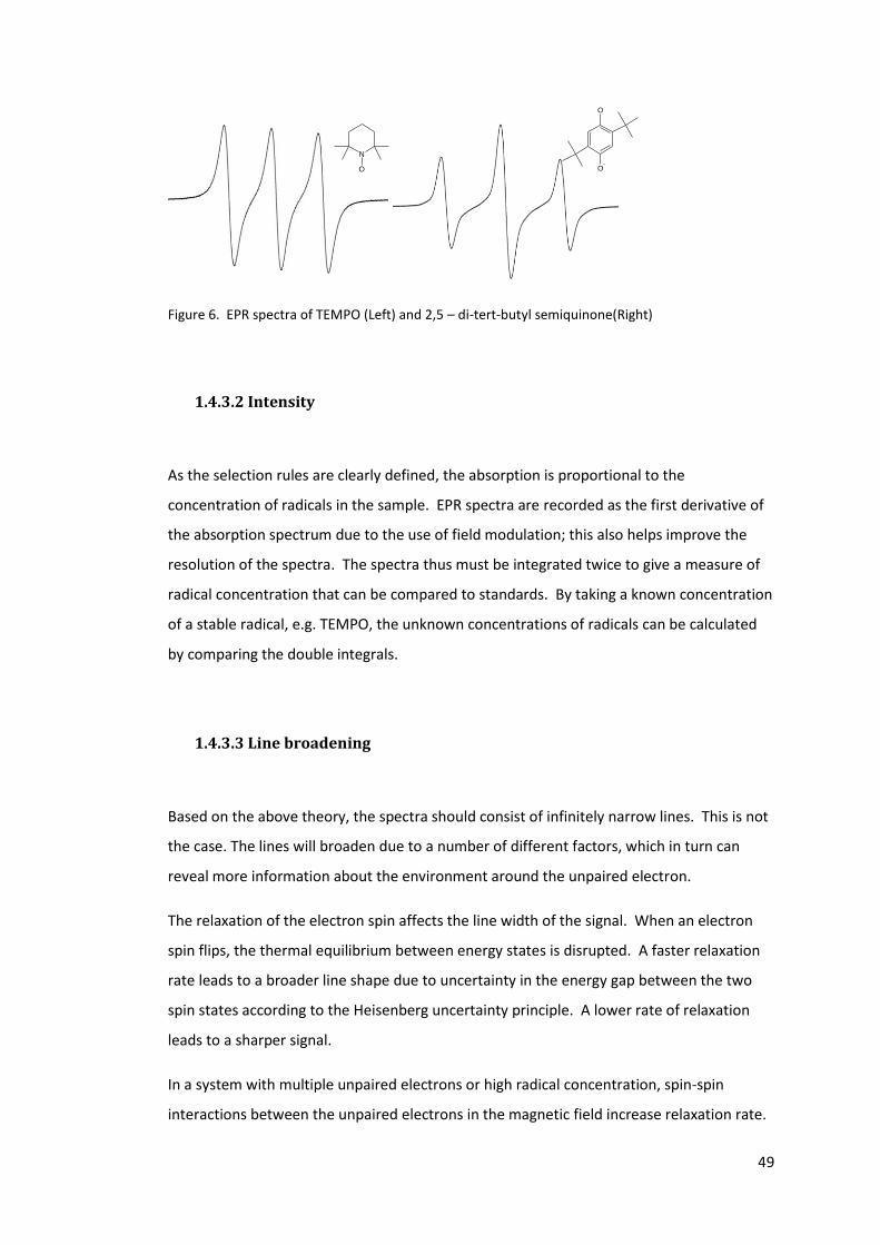
49
Figure 6. EPR spectra of TEMPO (Left) and 2,5 – di-tert-butyl semiquinone(Right)
1.4.3.2 Intensity
As the selection rules are clearly defined, the absorption is proportional to the
concentration of radicals in the sample. EPR spectra are recorded as the first derivative of
the absorption spectrum due to the use of field modulation; this also helps improve the
resolution of the spectra. The spectra thus must be integrated twice to give a measure of
radical concentration that can be compared to standards. By taking a known concentration
of a stable radical, e.g. TEMPO, the unknown concentrations of radicals can be calculated
by comparing the double integrals.
1.4.3.3 Line broadening
Based on the above theory, the spectra should consist of infinitely narrow lines. This is not
the case. The lines will broaden due to a number of different factors, which in turn can
reveal more information about the environment around the unpaired electron.
The relaxation of the electron spin affects the line width of the signal. When an electron
spin flips, the thermal equilibrium between energy states is disrupted. A faster relaxation
rate leads to a broader line shape due to uncertainty in the energy gap between the two
spin states according to the Heisenberg uncertainty principle. A lower rate of relaxation
leads to a sharper signal.
In a system with multiple unpaired electrons or high radical concentration, spin-spin
interactions between the unpaired electrons in the magnetic field increase relaxation rate.
N
O
O
O-
50
This increases the line broadening. For a system with a high enough radical concentration,
the analysis of line broadening can be used to determine radical concentrations.
1.5 Aims of the study
The above literature displays the current understanding and rationale for the inhibition of
spontaneous polymerisation. As legislation changes throughout the world, the tools
available to inhibit this polymerisation will also change. As stated above, DNBP (Section
1.3.1.3, page 39) is a common industrial polymerisation inhibitor. However, this inhibitor is
scheduled to cease production due to the changes in legislation. Therefore a new method
of inhibiting spontaneous polymerisation is needed. The overall aim of this research is to
develop improved mechanistic understanding of the action of polymerisation inhibitors
which will in the long term facilitate development of new inhibitors.
The study breaks down into two areas. The first objective was to investigate the
mechanism of polymerisation inhibition by nitrophenols (such as DNBP). This will require
the development and use of a method for determining the onset of polymerisation after
inhibition, so that structurally related molecules can be screened to observe trends in the
inhibition efficiency. Also, the determination of inhibition products would also be an area
for investigation in order to provide further details about the inhibition mechanism.
The second area is to evaluate and study the inhibition of spontaneous polymerisation by a
potential new inhibitor system. A charge transfer complex between quinones and amines,
first reported by Yassin and Rizk61 has been proposed. Their proposal included identifying
the chloranil radical anion part of the complex as the inhibiting species. The stability and
properties of the chloranil radical anion, including potential inhibition ability, should serve
as the initial investigation.
51
2. Nitrophenols as inhibitors
2.1 Monitoring polymerisation
To investigate the inhibition of spontaneous polymerisation, a method of monitoring the
rate of polymerisation and determining events, such as the onset of polymerisation after
inhibition, needs to be determined. The choice of method will be determined by how
appropriate it is when applied to spontaneous polymerisation, and practical reasons such
as cost. Fortunately, there are many methods to choose from.
The simplest, and least informative is to take an inhibited sample of monomer, heat it and
observe when it becomes a solid. Comparing the inhibited samples to uninhibited
monomer will make it possible to distinguish between compounds that inhibit and those
that do not, but nothing else. The concentration of the inhibitor needs to be relatively high
in order to observe inhibition. This means any expensive or difficult to synthesise
molecules could not be tested for inhibition properties. This approach is also labour
intensive as the samples will need constant monitoring for accurate results.
The results in Table 1 show possible trends in inhibition activity determined by this method.
For example, 2-nitrophenol inhibits far more than 3-nitrophenol, 4-nitrophenol and
nitrobenzene, with the latter three molecules showing similar activity. The difference in
position of the nitro group therefore gives rise to increased inhibition efficiency.
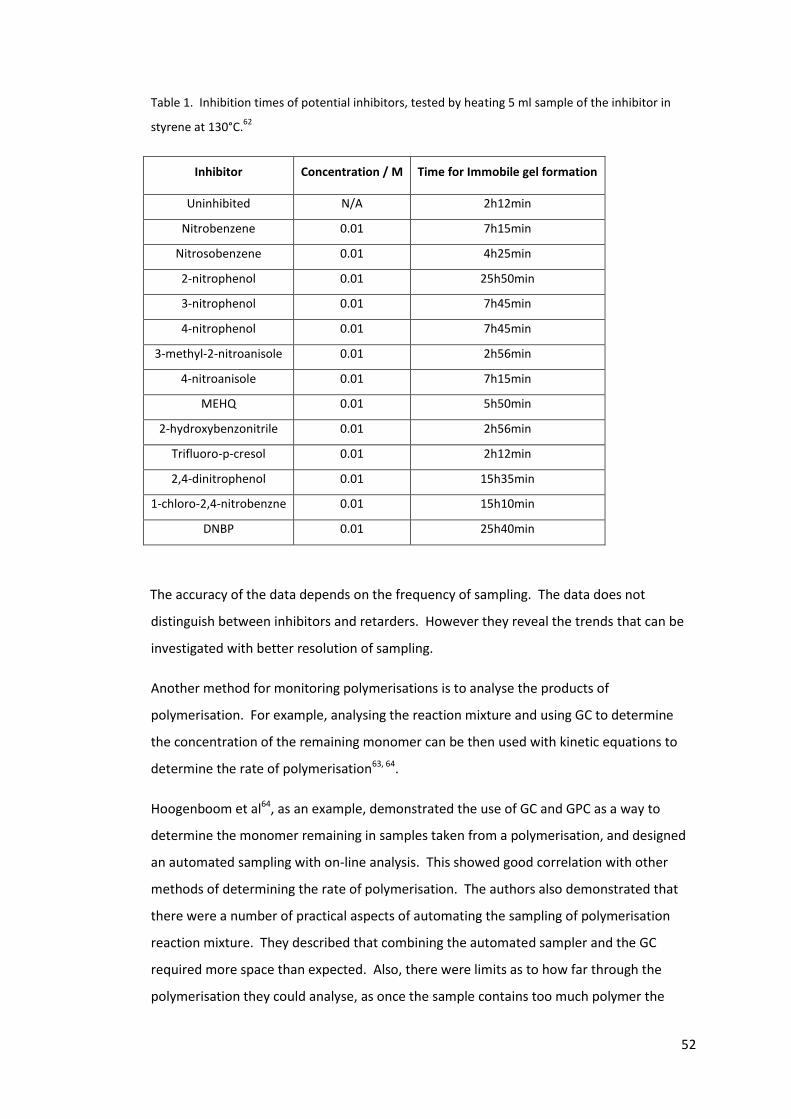
52
Table 1. Inhibition times of potential inhibitors, tested by heating 5 ml sample of the inhibitor in
styrene at 130°C.62
Inhibitor Concentration / M Time for Immobile gel formation
Uninhibited N/A 2h12min
Nitrobenzene 0.01 7h15min
Nitrosobenzene 0.01 4h25min
2-nitrophenol 0.01 25h50min
3-nitrophenol 0.01 7h45min
4-nitrophenol 0.01 7h45min
3-methyl-2-nitroanisole 0.01 2h56min
4-nitroanisole 0.01 7h15min
MEHQ 0.01 5h50min
2-hydroxybenzonitrile 0.01 2h56min
Trifluoro-p-cresol 0.01 2h12min
2,4-dinitrophenol 0.01 15h35min
1-chloro-2,4-nitrobenzne 0.01 15h10min
DNBP 0.01 25h40min
The accuracy of the data depends on the frequency of sampling. The data does not
distinguish between inhibitors and retarders. However they reveal the trends that can be
investigated with better resolution of sampling.
Another method for monitoring polymerisations is to analyse the products of
polymerisation. For example, analysing the reaction mixture and using GC to determine
the concentration of the remaining monomer can be then used with kinetic equations to
determine the rate of polymerisation63, 64.
Hoogenboom et al64, as an example, demonstrated the use of GC and GPC as a way to
determine the monomer remaining in samples taken from a polymerisation, and designed
an automated sampling with on-line analysis. This showed good correlation with other
methods of determining the rate of polymerisation. The authors also demonstrated that
there were a number of practical aspects of automating the sampling of polymerisation
reaction mixture. They described that combining the automated sampler and the GC
required more space than expected. Also, there were limits as to how far through the
polymerisation they could analyse, as once the sample contains too much polymer the
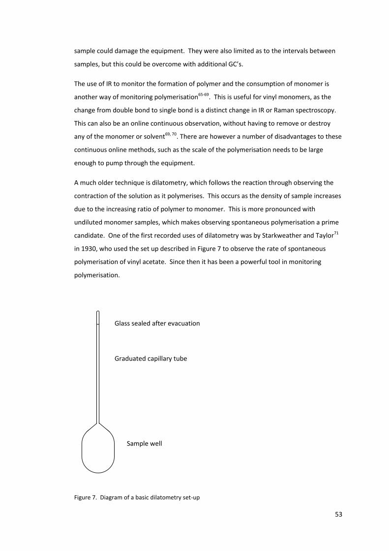
53
sample could damage the equipment. They were also limited as to the intervals between
samples, but this could be overcome with additional GC’s.
The use of IR to monitor the formation of polymer and the consumption of monomer is
another way of monitoring polymerisation65-69. This is useful for vinyl monomers, as the
change from double bond to single bond is a distinct change in IR or Raman spectroscopy.
This can also be an online continuous observation, without having to remove or destroy
any of the monomer or solvent69, 70. There are however a number of disadvantages to these
continuous online methods, such as the scale of the polymerisation needs to be large
enough to pump through the equipment.
A much older technique is dilatometry, which follows the reaction through observing the
contraction of the solution as it polymerises. This occurs as the density of sample increases
due to the increasing ratio of polymer to monomer. This is more pronounced with
undiluted monomer samples, which makes observing spontaneous polymerisation a prime
candidate. One of the first recorded uses of dilatometry was by Starkweather and Taylor71
in 1930, who used the set up described in Figure 7 to observe the rate of spontaneous
polymerisation of vinyl acetate. Since then it has been a powerful tool in monitoring
polymerisation.
Figure 7. Diagram of a basic dilatometry set-up
Graduated capillary tube
Glass sealed after evacuation
Sample well
54
Dilatometry can be adapted to run under the complete exclusion of air, as described by
authors such as Goldfinger and Lauterbach72, and Schulz and Harborth73. These methods
involve standard practices in removing oxygen from solutions, and then sealing them into
the glass apparatus under vacuum. Although this means that the dilatometry part of the
glassware is not recyclable, the apparatus is relatively cheap to make, making this method
viable.
As the aim of this project requires a comparative study of the rates of polymerisation in the
presence of different inhibitors, dilatometry was chosen as the main method of analysis.
2.2 Dilatometry
As described above, dilatometry is a useful tool for observing the polymerisation of a
material. Here, this technique has been utilised to determine the onset of polymerisation
after an inhibitor has been consumed. This technique also showed the change in the rate
of polymerisation.
The first dilatometry experiments for polymerisation in the literature utilised a capillary
tube attached to a large well filled with monomer.71-74 The large volume increases the
observable change in height of the monomer meniscus. Also, the narrower the capillary
leads to a greater the change in meniscus height. As the mass and volume remain the
same, and the capillary tube is of uniform dimension, then linear rates of change will be
observed as linear rates of change of height.
Using the known densities of polymer and monomer, the change in height for complete
polymerisation can be calculated. This has been determined in the literature for a range of
monomers at room temperature75 and given in Table 2.
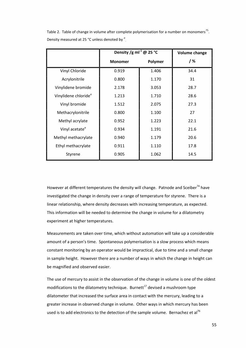
55
Table 2. Table of change in volume after complete polymerisation for a number on monomers75
.
Density measured at 25 °C unless denoted by a
.
Density /g ml-1 @ 25 °C Volume change
/ % Monomer Polymer
Vinyl Chloride 0.919 1.406 34.4
Acrylonitrile 0.800 1.170 31
Vinylidene bromide 2.178 3.053 28.7
Vinylidene chloridea 1.213 1.710 28.6
Vinyl bromide 1.512 2.075 27.3
Methacrylonitrile 0.800 1.100 27
Methyl acrylate 0.952 1.223 22.1
Vinyl acetatea 0.934 1.191 21.6
Methyl methacrylate 0.940 1.179 20.6
Ethyl methacrylate 0.911 1.110 17.8
Styrene 0.905 1.062 14.5
However at different temperatures the density will change. Patnode and Sceiber74 have
investigated the change in density over a range of temperature for styrene. There is a
linear relationship, where density decreases with increasing temperature, as expected.
This information will be needed to determine the change in volume for a dilatometry
experiment at higher temperatures.
Measurements are taken over time, which without automation will take up a considerable
amount of a person’s time. Spontaneous polymerisation is a slow process which means
constant monitoring by an operator would be impractical, due to time and a small change
in sample height. However there are a number of ways in which the change in height can
be magnified and observed easier.
The use of mercury to assist in the observation of the change in volume is one of the oldest
modifications to the dilatometry technique. Burnett17 devised a mushroom type
dilatometer that increased the surface area in contact with the mercury, leading to a
greater increase in observed change in volume. Other ways in which mercury has been
used is to add electronics to the detection of the sample volume. Bernachez et al76
56
constructed a mercury manometer in which the resistance of a wire stretched into the
mercury column is varied by changes in the height of the mercury. With a constant
current, there is a linear relationship between the signal detected and change in height of
the mercury column. The obvious disadvantage of this technique, and the reason it is very
rarely used, is due to the toxicity and hazards associated with mercury.
A technique used more recently is based on capacitance. This makes use of changing the
distance between two electrodes. As the distance between the electrodes increases, the
capacitance changes. Frey et al77 describe using mercury within a capillary with a metal
outer electrode. As the volume of the sample changes, the volume of mercury within the
cylindrical electrode increases, leading to change in capacitance. This change can be
monitored, leading to changes in meniscus position beyond 100 nm being observable,
providing the meniscus of the mercury is within the electrode.
Another capacitance method has been described by Neumeier et al77 which uses a unit
built of quartz to minimise the thermal expansion of the device itself. They have observed
the changes in volume due to thermal expansion. They have observed sub Angstrom
changes in the height measurement and have used the equipment over a temperature
range of 5 K to 350 K. The use of capacitance in dilatometry to observe the changes in
volume and to automate the process is impressive as to what can be achieved.
2.2.1 Disadvantages of current methods
The traditional setup to monitor polymerisation requires large volumes of inhibited
monomer to work effectively. This is not preferable if using dilatometry for proof of
concept experiments where a small amount of inhibitor may be available.
A common component of a traditional dilatometry setup involves mercury as a way of
observing the volume change. This is toxic and is being phased out of modern laboratories.
Through-put of these techniques is limited. Only one sample at a time can be run in the
individual setups. The computer recording the data from the instruments could easily
record more than one data stream, but that would require a second piece of equipment to
be purchased to make the measurements.
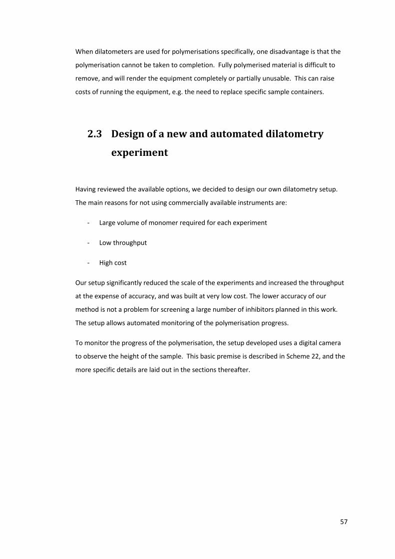
57
When dilatometers are used for polymerisations specifically, one disadvantage is that the
polymerisation cannot be taken to completion. Fully polymerised material is difficult to
remove, and will render the equipment completely or partially unusable. This can raise
costs of running the equipment, e.g. the need to replace specific sample containers.
2.3 Design of a new and automated dilatometry
experiment
Having reviewed the available options, we decided to design our own dilatometry setup.
The main reasons for not using commercially available instruments are:
- Large volume of monomer required for each experiment
- Low throughput
- High cost
Our setup significantly reduced the scale of the experiments and increased the throughput
at the expense of accuracy, and was built at very low cost. The lower accuracy of our
method is not a problem for screening a large number of inhibitors planned in this work.
The setup allows automated monitoring of the polymerisation progress.
To monitor the progress of the polymerisation, the setup developed uses a digital camera
to observe the height of the sample. This basic premise is described in Scheme 22, and the
more specific details are laid out in the sections thereafter.
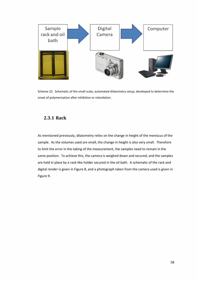
58
Scheme 22. Schematic of the small scale, automated dilatometry setup, developed to determine the
onset of polymerisation after inhibition or retardation.
2.3.1 Rack
As mentioned previously, dilatometry relies on the change in height of the meniscus of the
sample. As the volumes used are small, the change in height is also very small. Therefore
to limit the error in the taking of the measurement, the samples need to remain in the
same position. To achieve this, the camera is weighed down and secured, and the samples
are held in place by a rack-like holder secured in the oil bath. A schematic of the rack and
digital render is given in Figure 8, and a photograph taken from the camera used is given in
Figure 9.
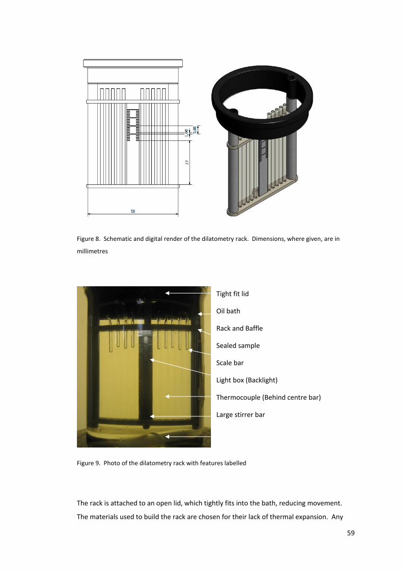
59
Figure 8. Schematic and digital render of the dilatometry rack. Dimensions, where given, are in
millimetres
Figure 9. Photo of the dilatometry rack with features labelled
The rack is attached to an open lid, which tightly fits into the bath, reducing movement.
The materials used to build the rack are chosen for their lack of thermal expansion. Any
Tight fit lid
Oil bath
Rack and Baffle
Sealed sample
Scale bar
Light box (Backlight)
Thermocouple (Behind centre bar)
Large stirrer bar
60
thermal expansion is detectable by the analysis of the images, and can also lead to the
samples becoming loose in the holder, and moving around in the loose space.
The rest of the equipment is either weighed down or positioned in a fume hood on rubber
feet or other surfaces where nothing is likely to slip or move due to vibrations. Also, as the
system is automated, the samples are ran over night or over weekends, as to avoid
vibrations and interference from colleagues working around the equipment.
The rack is designed to submerge the samples completely. In initial experiments where
samples were partially submerged, monomer condensed at the top of the sealed tube.
This gave varying rates of change in height, which was not due to the polymerisation.
Therefore, complete submersion is required to maintain accuracy and reproducibility.
2.3.2 Oil bath and heating
The oil bath is heated by a standard stirrer hotplate. A large stirrer bar is used to mix and
maintain a constant temperature throughout the oil. However, in the initial development,
this was not enough to limit thermal variation in oil. There are ways of improving the heat
transfer through the oil bath, such as the use of different agitators (overhead stirrers with
different propeller type blades rather than a magnetic stirrer bar) and vessel shapes and
sizes78, 79. However, the setup is restricted in what can be used, due to the need for visual
measurements. A method of maintaining a constant temperature through a fluid in a
stirred vessel is to add barriers that disrupt the flow of the fluid. These are called baffles.
The final holder design acts as a baffle sufficient for the experiment. In this set up the
thermal variation in the oil was ±0.2°C from the set temperature.
The thermocouple is held behind the scale bar in the rack holder, so that it is in the optimal
position and also to maximise the space in the images. Another detail is that the speed of
the stirrer bar needs to be optimised so that there is sufficient mixing, but not so much as
to cause a vortex to form obscuring the samples and exposing the tops of the samples to
the cooler air.
The procedure for starting a dilatometry run for this equipment has been refined to give
the reproducible and accurate results. The oil bath is “over-heated” before a run; that is,
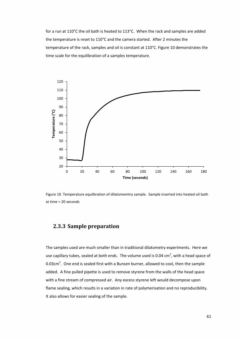
61
for a run at 110°C the oil bath is heated to 113°C. When the rack and samples are added
the temperature is reset to 110°C and the camera started. After 2 minutes the
temperature of the rack, samples and oil is constant at 110°C. Figure 10 demonstrates the
time scale for the equilibration of a samples temperature.
Figure 10. Temperature equilbration of dilatomemtry sample. Sample inserted into heated oil bath
at time = 20 seconds
2.3.3 Sample preparation
The samples used are much smaller than in traditional dilatometry experiments. Here we
use capillary tubes, sealed at both ends. The volume used is 0.04 cm3, with a head space of
0.03cm3. One end is sealed first with a Bunsen burner, allowed to cool, then the sample
added. A fine pulled pipette is used to remove styrene from the walls of the head space
with a fine stream of compressed air. Any excess styrene left would decompose upon
flame sealing, which results in a variation in rate of polymerisation and no reproducibility.
It also allows for easier sealing of the sample.
20
30
40
50
60
70
80
90
100
110
120
0 20 40 60 80 100 120 140 160 180
Tem
pe
ratu
re (
°C)
Time (seconds)
62
2.3.4 Camera and lighting
A commercially available 4-megapixel digital camera was used to observe the sample rack.
The model has a built in remote shooting function combined with a timer function, used to
take an image at regular intervals automatically. The resolution of the camera is high
enough to distinguish the small change in height as the polymerisation takes place.
The total change in height can be calculated using the densities of styrene and polystyrene
at the temperature the dilatometer is run at. Using information published by Patnode and
Scheiber74, the densities of styrene and polystyrene at 110 °C are 0.825 g ml-1 and 1.016 g
ml-1, respectively. From this the change in volume can be determined as 18.8%. The total
height of a sample in an image is on average 950 pixels. Therefore the total change in
height in an image for a sample of styrene is 178 pixels. This means 1 % polymerisation is
about 1-2 pixels, giving good resolution.
To increase the height of the sample in the image, the camera could be moved closer to the
oil bath. Unfortunately the heat from the hot plate would damage the camera, but it was
left as close as possible. From the above calculation, the resolution was deemed good
enough to distinguish inhibition times and retarded rates.
The camera also has a “macro” function, designed to allow picture of objects close to the
camera. Without this, the images are blurred, leading to noise in the analysis.
In order for the meniscus to be easily visible, a light box is used on its side as a back light.
This makes the volume of the sample clearly visible for the analysis.
2.3.5 Data analysis
The images are analysed by a purpose written program. The program requires a user to
determine where the menisci of the samples are in the images, and where the bottom of
the sample is. With this information, the program calculates the relative height of the
samples in relation to the first image. This is why it is vital the sample rack is immobile, as
63
any movement means the positions of the samples in the later images are no longer the
same, and the relative height is incorrect.
The original program used at the start of the study would take as long to analyse images as
it did to collect them. The program underwent a number of improvements, to make more
efficient use of time.
Typically more than one sample of inhibitor being investigated will be run at a time,
alongside duplicates of uninhibited monomer. The results for the uninhibited monomer,
and the duplication of all samples in a run can be used to eliminate any anomalies, e.g.
heating not working correctly or unwanted movement of the camera.
2.3.6 Standards and calibration of the new setup
In order to determine the stability of the equipment and to demonstrate that any change in
the values calculated are due to polymerisation, toluene was used as an example of a non-
polymerisable sample. Figure 11demonstrates the variation in the meniscus height
measured. Again, all values are relative to the first image. There is very little variation in
height.
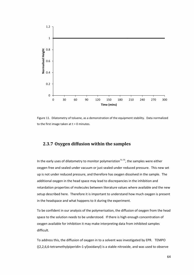
64
Figure 11. Dilatometry of toluene, as a demonstration of the equipment stability. Data normalized
to the first image taken at t = 0 minutes.
2.3.7 Oxygen diffusion within the samples
In the early uses of dilatometry to monitor polymeristion71-75, the samples were either
oxygen free and sealed under vacuum or just sealed under reduced pressure. This new set
up is not under reduced pressure, and therefore has oxygen dissolved in the sample. The
additional oxygen in the head space may lead to discrepancies in the inhibition and
retardation properties of molecules between literature values where available and the new
setup described here. Therefore it is important to understand how much oxygen is present
in the headspace and what happens to it during the experiment.
To be confident in our analysis of the polymerisation, the diffusion of oxygen from the head
space to the solution needs to be understood. If there is high enough concentration of
oxygen available for inhibition it may make interpreting data from inhibited samples
difficult.
To address this, the diffusion of oxygen in to a solvent was investigated by EPR. TEMPO
((2,2,6,6-tetramethylpiperidin-1-yl)oxidanyl) is a stable nitroxide, and was used to observe
0
0.2
0.4
0.6
0.8
1
1.2
0 30 60 90 120 150 180 210 240 270 300
No
rmai
lse
d H
eig
ht
Time (mins)
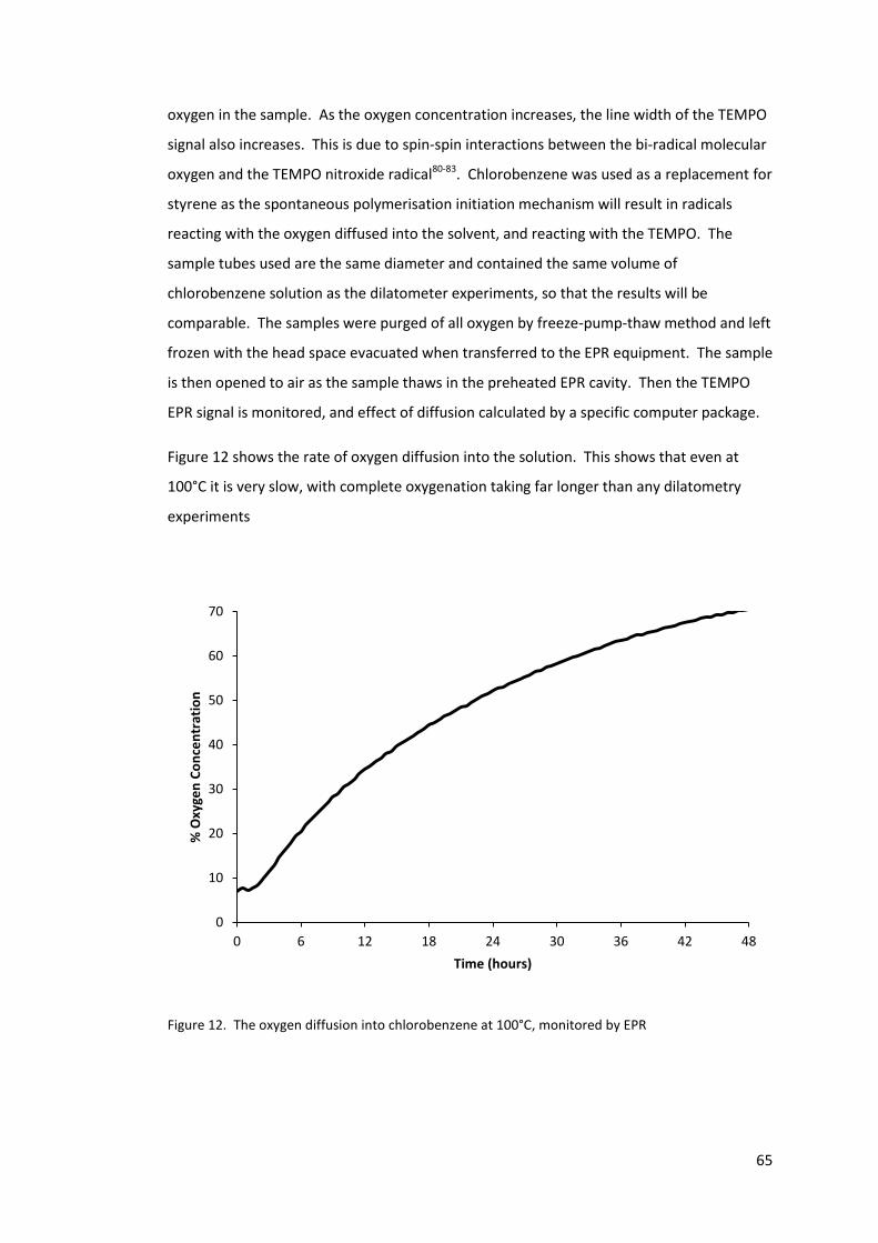
65
oxygen in the sample. As the oxygen concentration increases, the line width of the TEMPO
signal also increases. This is due to spin-spin interactions between the bi-radical molecular
oxygen and the TEMPO nitroxide radical80-83. Chlorobenzene was used as a replacement for
styrene as the spontaneous polymerisation initiation mechanism will result in radicals
reacting with the oxygen diffused into the solvent, and reacting with the TEMPO. The
sample tubes used are the same diameter and contained the same volume of
chlorobenzene solution as the dilatometer experiments, so that the results will be
comparable. The samples were purged of all oxygen by freeze-pump-thaw method and left
frozen with the head space evacuated when transferred to the EPR equipment. The sample
is then opened to air as the sample thaws in the preheated EPR cavity. Then the TEMPO
EPR signal is monitored, and effect of diffusion calculated by a specific computer package.
Figure 12 shows the rate of oxygen diffusion into the solution. This shows that even at
100°C it is very slow, with complete oxygenation taking far longer than any dilatometry
experiments
Figure 12. The oxygen diffusion into chlorobenzene at 100°C, monitored by EPR
0
10
20
30
40
50
60
70
0 6 12 18 24 30 36 42 48
% O
xyge
n C
on
cen
trat
ion
Time (hours)
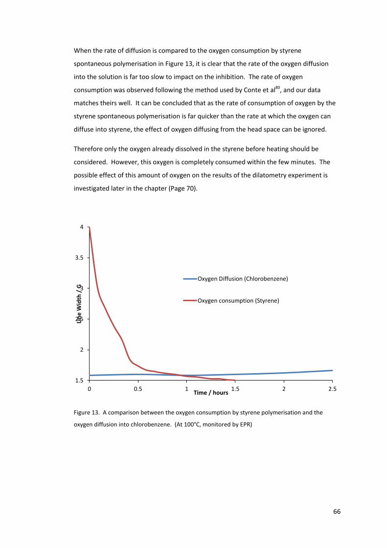
66
When the rate of diffusion is compared to the oxygen consumption by styrene
spontaneous polymerisation in Figure 13, it is clear that the rate of the oxygen diffusion
into the solution is far too slow to impact on the inhibition. The rate of oxygen
consumption was observed following the method used by Conte et al80, and our data
matches theirs well. It can be concluded that as the rate of consumption of oxygen by the
styrene spontaneous polymerisation is far quicker than the rate at which the oxygen can
diffuse into styrene, the effect of oxygen diffusing from the head space can be ignored.
Therefore only the oxygen already dissolved in the styrene before heating should be
considered. However, this oxygen is completely consumed within the few minutes. The
possible effect of this amount of oxygen on the results of the dilatometry experiment is
investigated later in the chapter (Page 70).
Figure 13. A comparison between the oxygen consumption by styrene polymerisation and the
oxygen diffusion into chlorobenzene. (At 100°C, monitored by EPR)
1.5
2
2.5
3
3.5
4
0 0.5 1 1.5 2 2.5
Lin
e W
idth
/ G
Time / hours
Oxygen Diffusion (Chlorobenzene)
Oxygen consumption (Styrene)
67
2.4 Case studies for proof of concept
2.4.1 Uninhibited styrene
Styrene has an understood spontaneous polymerisation mechanism19, and makes a good
candidate for testing our dilatometry set up. The change in height due to polymerisation
calculated from the data provided by Partnode and Sciber74 show that complete
polymerisation will reduce the height by 18.8 %. However, this set up reaches completion
at a slightly higher meniscus height drop of 20%, suggesting over 100% conversion.
The reason for this apparently anomalous conversion of monomer to polymer is possibly
because the shape of the meniscus may change during polymerisation. In larger
dilatometry setups, the meniscus will be flat apart from a small area of the surface that will
curve up the wall of the glassware. In a smaller sample, the meniscus is mostly curved due
to the same effect. If the shape of the curve remained consistent throughout, the change
in height after 100% conversion would be identical to literature. However, as the
polymerisation progresses, the viscosity of the sample will increase, which will increase the
curvature of the meniscus. At this point, a greater volume of the monomer will no longer
be accounted for by the camera, and will thus result in an apparent conversion over 100%.
We note that this effect is relatively small and is only significant at high degree of
polymerisation. As the rates of polymerisation obtained from the dilatometer are self-
consistent, a 20% change in height in our setup is used in this thesis as a point for 100%
conversion of monomer to polymer (Figure 14).
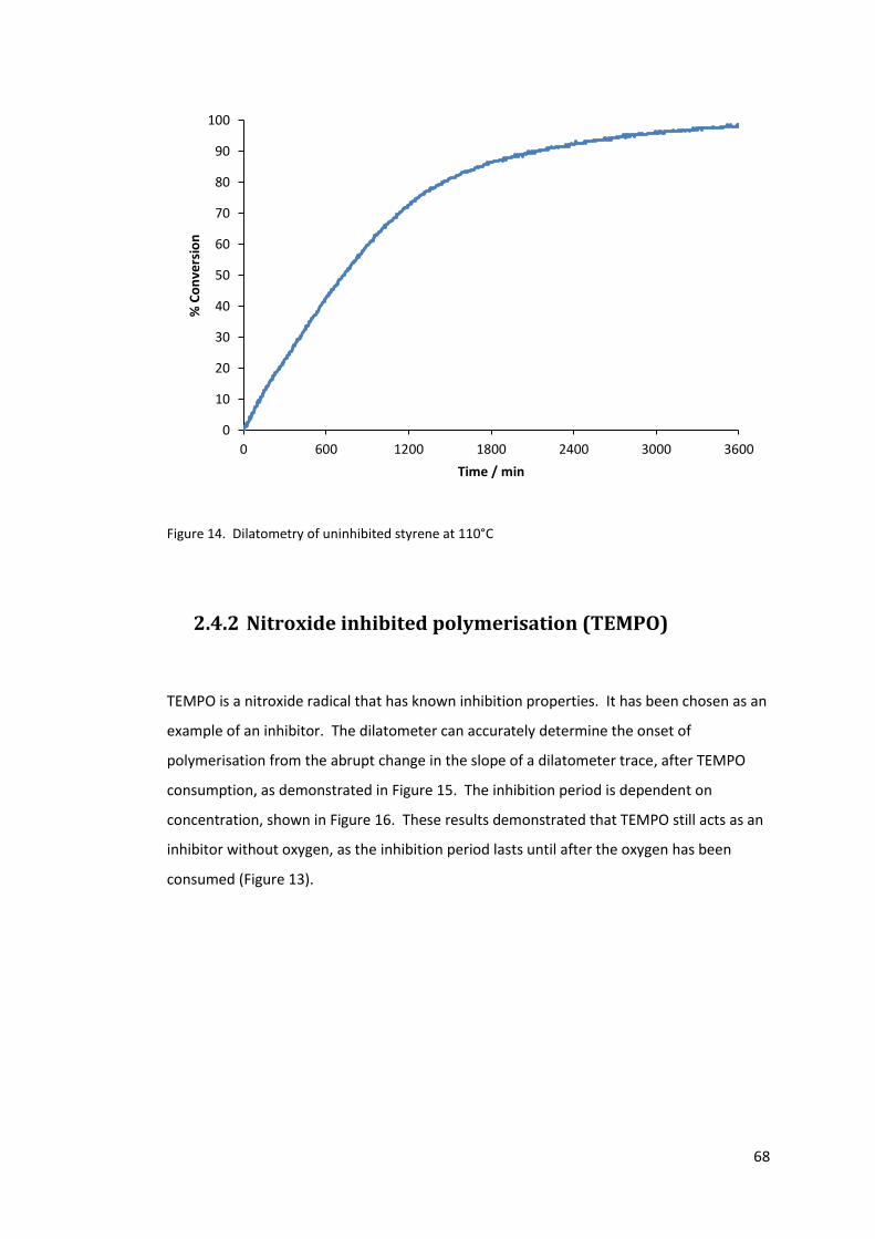
68
Figure 14. Dilatometry of uninhibited styrene at 110°C
2.4.2 Nitroxide inhibited polymerisation (TEMPO)
TEMPO is a nitroxide radical that has known inhibition properties. It has been chosen as an
example of an inhibitor. The dilatometer can accurately determine the onset of
polymerisation from the abrupt change in the slope of a dilatometer trace, after TEMPO
consumption, as demonstrated in Figure 15. The inhibition period is dependent on
concentration, shown in Figure 16. These results demonstrated that TEMPO still acts as an
inhibitor without oxygen, as the inhibition period lasts until after the oxygen has been
consumed (Figure 13).
0
10
20
30
40
50
60
70
80
90
100
0 600 1200 1800 2400 3000 3600
% C
on
vers
ion
Time / min
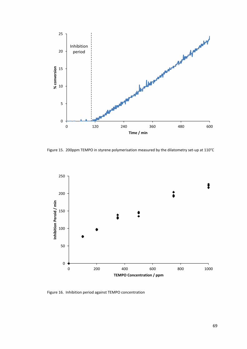
69
Figure 15. 200ppm TEMPO in styrene polymerisation measured by the dilatometry set-up at 110°C
Figure 16. Inhibition period against TEMPO concentration
0
5
10
15
20
25
0 120 240 360 480 600
% c
on
vers
ion
Time / min
Inhibition period
0
50
100
150
200
250
0 200 400 600 800 1000
Inh
ibit
ion
Pe
roid
/ m
in
TEMPO Concentration / ppm
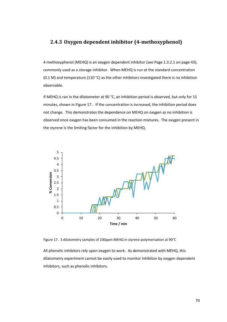
70
2.4.3 Oxygen dependent inhibitor (4-methoxyphenol)
4-methoxyphenol (MEHQ) is an oxygen dependent inhibitor (see Page 1.3.2.1 on page 43),
commonly used as a storage inhibitor. When MEHQ is run at the standard concentration
(0.1 M) and temperature (110 °C) as the other inhibitors investigated there is no inhibition
observable.
If MEHQ is ran in the dilatometer at 90 °C, an inhibition period is observed, but only for 15
minutes, shown in Figure 17.. If the concentration is increased, the inhibition period does
not change. This demonstrates the dependence on MEHQ on oxygen as no inhibition is
observed once oxygen has been consumed in the reaction mixtures. The oxygen present in
the styrene is the limiting factor for the inhibition by MEHQ.
Figure 17. 3 dilatometry samples of 100ppm MEHQ in styrene polymerisation at 90°C
All phenolic inhibitors rely upon oxygen to work. As demonstrated with MEHQ, this
dilatometry experiment cannot be easily used to monitor inhibiton by oxygen dependent
inhibitors, such as phenolic inhibitors.
0
0.5
1
1.5
2
2.5
3
3.5
4
4.5
5
0 10 20 30 40 50 60
% C
on
vers
ion
Time / min
71
2.4.4 Conclusions on the new dilatometry set-up
A new dilatometry set has been developed, that uses a small amount (0.03 ml) of inhibited
sample. The sample preparation is simple and the data acquisition and analysis are
completely automated. Multiple samples can be run simultaneously making this method
efficient. As the sample tubes are inexpensive, the polymerisations can be run to
completion, without worry of loss of equipment. The method can detect long inhibition
periods and can distinguish between inhibitors and retarders.
The rate of oxygen diffusion into chlorobenzene has been observed to be extremely slow at
110 °C. The rate of oxygen consumption by styrene has also been observed by a similar
method. As the rate of diffusion is much slower than the rate of consumption, the effect of
oxygen diffusing into the solution from the headspace of the dilatometry capillary has been
deemed insignificant and can be ignored.
Toluene has been run alongside styrene as an example of a non-polymerisable material,
and showed no change in meniscus height when monitored by the dilatometry setup. This
demonstrates that the change in height shown by styrene is due to polymerisation.
TEMPO has been used as an example of a polymerisation inhibitor. The concentration
dependence of the inhibition time has been observed by the dilatometry experiment, and
proved the concept of determining the onset of polymerisation after inhibition.
MEHQ was chosen as an example of an oxygen dependent inhibitor. As demonstrated
earlier, the oxygen is consumed within the first few minutes. At 110 °C there was no
inhibition observable. At 90 °C, there was a short inhibition period of 15 min. At the
concentration used, this is a demonstration of the limits of the dilatometry experiment.
The method cannot be used to observe oxygen dependent inhibitors. This will be a useful
tool for differentiating between inhibitors that need oxygen and those that do not.
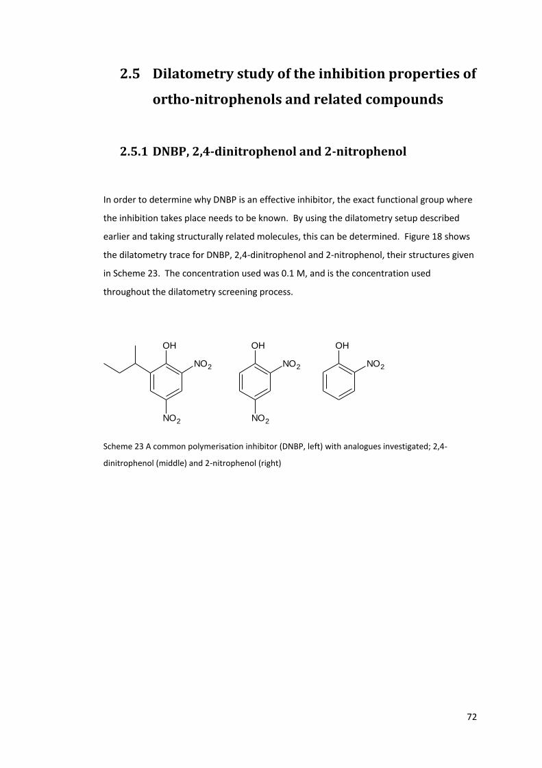
72
2.5 Dilatometry study of the inhibition properties of
ortho-nitrophenols and related compounds
2.5.1 DNBP, 2,4-dinitrophenol and 2-nitrophenol
In order to determine why DNBP is an effective inhibitor, the exact functional group where
the inhibition takes place needs to be known. By using the dilatometry setup described
earlier and taking structurally related molecules, this can be determined. Figure 18 shows
the dilatometry trace for DNBP, 2,4-dinitrophenol and 2-nitrophenol, their structures given
in Scheme 23. The concentration used was 0.1 M, and is the concentration used
throughout the dilatometry screening process.
Scheme 23 A common polymerisation inhibitor (DNBP, left) with analogues investigated; 2,4-
dinitrophenol (middle) and 2-nitrophenol (right)
OH
NO2
OH
NO2
NO2
OH
NO2
NO2
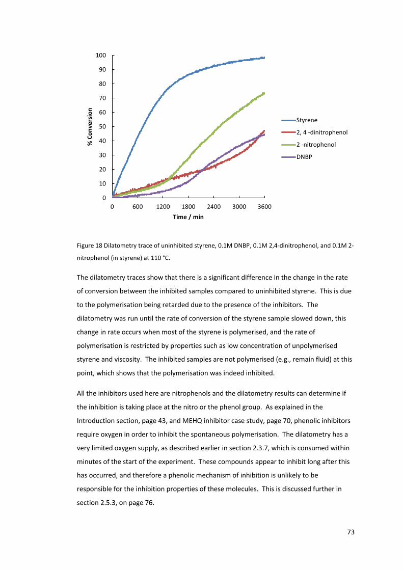
73
Figure 18 Dilatometry trace of uninhibited styrene, 0.1M DNBP, 0.1M 2,4-dinitrophenol, and 0.1M 2-
nitrophenol (in styrene) at 110 °C.
The dilatometry traces show that there is a significant difference in the change in the rate
of conversion between the inhibited samples compared to uninhibited styrene. This is due
to the polymerisation being retarded due to the presence of the inhibitors. The
dilatometry was run until the rate of conversion of the styrene sample slowed down, this
change in rate occurs when most of the styrene is polymerised, and the rate of
polymerisation is restricted by properties such as low concentration of unpolymerised
styrene and viscosity. The inhibited samples are not polymerised (e.g., remain fluid) at this
point, which shows that the polymerisation was indeed inhibited.
All the inhibitors used here are nitrophenols and the dilatometry results can determine if
the inhibition is taking place at the nitro or the phenol group. As explained in the
Introduction section, page 43, and MEHQ inhibitor case study, page 70, phenolic inhibitors
require oxygen in order to inhibit the spontaneous polymerisation. The dilatometry has a
very limited oxygen supply, as described earlier in section 2.3.7, which is consumed within
minutes of the start of the experiment. These compounds appear to inhibit long after this
has occurred, and therefore a phenolic mechanism of inhibition is unlikely to be
responsible for the inhibition properties of these molecules. This is discussed further in
section 2.5.3, on page 76.
0
10
20
30
40
50
60
70
80
90
100
0 600 1200 1800 2400 3000 3600
% C
on
vers
ion
Time / min
Styrene
2, 4 -dinitrophenol
2 -nitrophenol
DNBP
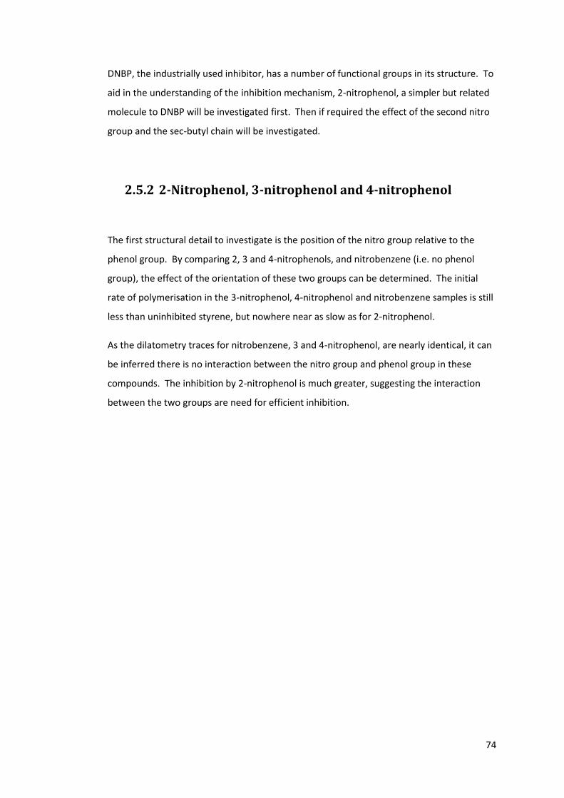
74
DNBP, the industrially used inhibitor, has a number of functional groups in its structure. To
aid in the understanding of the inhibition mechanism, 2-nitrophenol, a simpler but related
molecule to DNBP will be investigated first. Then if required the effect of the second nitro
group and the sec-butyl chain will be investigated.
2.5.2 2-Nitrophenol, 3-nitrophenol and 4-nitrophenol
The first structural detail to investigate is the position of the nitro group relative to the
phenol group. By comparing 2, 3 and 4-nitrophenols, and nitrobenzene (i.e. no phenol
group), the effect of the orientation of these two groups can be determined. The initial
rate of polymerisation in the 3-nitrophenol, 4-nitrophenol and nitrobenzene samples is still
less than uninhibited styrene, but nowhere near as slow as for 2-nitrophenol.
As the dilatometry traces for nitrobenzene, 3 and 4-nitrophenol, are nearly identical, it can
be inferred there is no interaction between the nitro group and phenol group in these
compounds. The inhibition by 2-nitrophenol is much greater, suggesting the interaction
between the two groups are need for efficient inhibition.
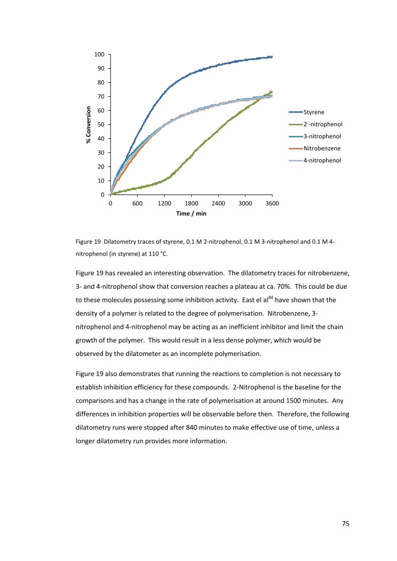
75
Figure 19 Dilatometry traces of styrene, 0.1 M 2-nitrophenol, 0.1 M 3-nitrophenol and 0.1 M 4-
nitrophenol (in styrene) at 110 °C.
Figure 19 has revealed an interesting observation. The dilatometry traces for nitrobenzene,
3- and 4-nitrophenol show that conversion reaches a plateau at ca. 70%. This could be due
to these molecules possessing some inhibition activity. East el al84 have shown that the
density of a polymer is related to the degree of polymerisation. Nitrobenzene, 3-
nitrophenol and 4-nitrophenol may be acting as an inefficient inhibitor and limit the chain
growth of the polymer. This would result in a less dense polymer, which would be
observed by the dilatometer as an incomplete polymerisation.
Figure 19 also demonstrates that running the reactions to completion is not necessary to
establish inhibition efficiency for these compounds. 2-Nitrophenol is the baseline for the
comparisons and has a change in the rate of polymerisation at around 1500 minutes. Any
differences in inhibition properties will be observable before then. Therefore, the following
dilatometry runs were stopped after 840 minutes to make effective use of time, unless a
longer dilatometry run provides more information.
0
10
20
30
40
50
60
70
80
90
100
0 600 1200 1800 2400 3000 3600
% C
on
vers
ion
Time / min
Styrene
2 -nitrophenol
3-nitrophenol
Nitrobenzene
4-nitrophenol

76
2.5.3 The structural group responsible for inhibition
DNBP contains two known inhibitor groups; nitro and phenol. It is not known if the two
inhibit separately, through their own separate mechanisms, of through an interaction of
the two groups. From the dilatometry experiment, comparing 2, 3 and 4-nitrophenols,
there appears to be a structural element to the inhibition efficacy.
Starting with the known mechanisms, phenolic inhibitors work through donating their
hydrogen to peroxyl radicals, as discussed by Levy at al55, 85, and described in the
introduction chapter (Section 1.3.2.1. on page 43). Levy et al discussed the properties of 4-
methoxyphenol (also called monomethyl ether hydroquinone or MEHQ) which is a
common storage inhibitor. They showed that MEHQ is only efficient in the presence of
oxygen. Their mechanism suggested that the initial step in the inhibition is due to the
initiator radical first reacting with oxygen dissolved in the monomer. Oxygen consumption
by monomers has been studied37, 56, 86, and has been used as a way of monitoring self-
polymerisation in stored monomers.
The peroxyl radical that forms is then quenched by phenols in the above examples, through
the donation of its phenolic hydrogen to form peroxide. The phenoxyl radical that is formed
is stabilised through resonance, and does not initiate polymerisation. This is depicted in
Scheme 24 and Scheme 25. The direct donation of the phenolic hydrogen to carbon-
centred radicals (3rd reaction in Scheme 24) is an insufficiently fast reaction to inhibit
polymerisation87, and hence phenolic inhibitors do not work in the absence of oxygen.
R O2R
OO
RO
O + Ph OHR
OOH + Ph O
Cannot initiate
Ph OHR
OOH
Ph O+ +R
Slow compared to rate of initiation
+
Scheme 24. Demonstration of phenolic inhibition mechanism55, 85
77
O
CH
O
CH
O
CH
O
Scheme 25. The resonance structures of a phenoxy radical
The lack of inhibition of styrene polymerisation by phenols in the absence of oxygen is
confirmed in this work. In the case of the dilatometry presented above, the experimental
setup has a limited supply of oxygen. This was investigated when the dilatometry setup
was developed (section 2.3.7 on page 64). MEHQ was shown not to inhibit styrene
polymerisation in the absence of oxygen (section 2.4.3 on page 70). The samples of 2-
nitrophenol, 2,4-dintrophenol and DNBP however showed strong inhibition properties in
the absence of oxygen, unlike MEHQ. This suggests that the nitrophenols may not inhibit
through the same mechanism as MEHQ. To summarise, the very fact that o-nitrophenols
are efficient polymerisation inhibitors in the absence of oxygen strongly suggests that their
inhibition mechanism is not based on the H abstraction from the OH group.
Another strong argument against nitrophenols acting as inhibitors through the OH group is
that the dilatometry traces for 3-, 4-nitrophenols and nitrobenzene are all very similar but
quite different from that of 2-nitrophenol (section 2.5.2 on page 74). In particular, the fact
that nitrobenzene and 3-nitrophenol show nearly identical dilatometry profiles which are
very different from that of 2-nitrophenol suggests that inhibition properties of
nitrobenzene and 3-nitrophenol are determined by the nitro group. The much higher
inhibition efficiency of 2-nitrophenol can be explained by either of the following
arguments:
- 2-nitrophenol inhibition properties are due to the OH group which is weaker due to
resonance stabilisation of the corresponding phenoxyl radical (Scheme 26), or
- 2-nitrophenol inhibition properties are due to the nitro group but are enhanced by
the presence of the OH group in the ortho-position.
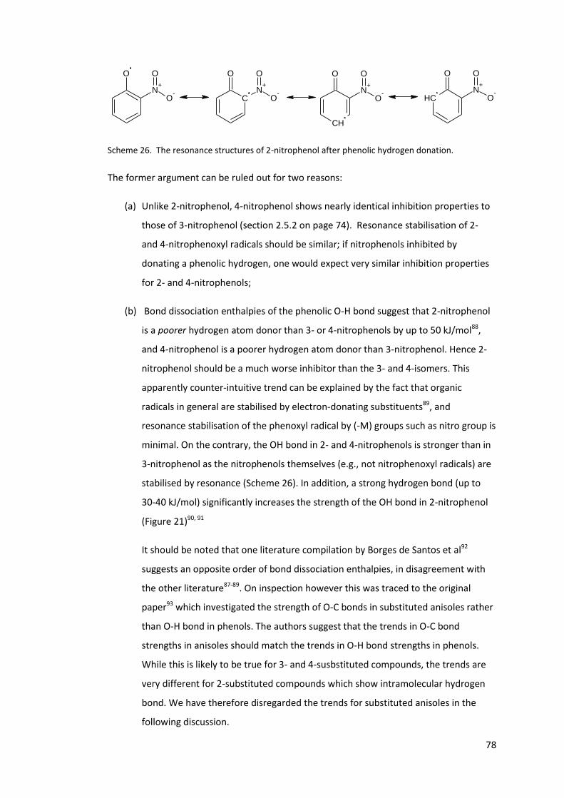
78
O
N+
O-
O
C
O
N+
O-
O
CH
O
N+
O-
O
CH
O
N+
O-
O
Scheme 26. The resonance structures of 2-nitrophenol after phenolic hydrogen donation.
The former argument can be ruled out for two reasons:
(a) Unlike 2-nitrophenol, 4-nitrophenol shows nearly identical inhibition properties to
those of 3-nitrophenol (section 2.5.2 on page 74). Resonance stabilisation of 2-
and 4-nitrophenoxyl radicals should be similar; if nitrophenols inhibited by
donating a phenolic hydrogen, one would expect very similar inhibition properties
for 2- and 4-nitrophenols;
(b) Bond dissociation enthalpies of the phenolic O-H bond suggest that 2-nitrophenol
is a poorer hydrogen atom donor than 3- or 4-nitrophenols by up to 50 kJ/mol88,
and 4-nitrophenol is a poorer hydrogen atom donor than 3-nitrophenol. Hence 2-
nitrophenol should be a much worse inhibitor than the 3- and 4-isomers. This
apparently counter-intuitive trend can be explained by the fact that organic
radicals in general are stabilised by electron-donating substituents89, and
resonance stabilisation of the phenoxyl radical by (-M) groups such as nitro group is
minimal. On the contrary, the OH bond in 2- and 4-nitrophenols is stronger than in
3-nitrophenol as the nitrophenols themselves (e.g., not nitrophenoxyl radicals) are
stabilised by resonance (Scheme 26). In addition, a strong hydrogen bond (up to
30-40 kJ/mol) significantly increases the strength of the OH bond in 2-nitrophenol
(Figure 21)90, 91
It should be noted that one literature compilation by Borges de Santos et al92
suggests an opposite order of bond dissociation enthalpies, in disagreement with
the other literature87-89. On inspection however this was traced to the original
paper93 which investigated the strength of O-C bonds in substituted anisoles rather
than O-H bond in phenols. The authors suggest that the trends in O-C bond
strengths in anisoles should match the trends in O-H bond strengths in phenols.
While this is likely to be true for 3- and 4-susbstituted compounds, the trends are
very different for 2-substituted compounds which show intramolecular hydrogen
bond. We have therefore disregarded the trends for substituted anisoles in the
following discussion.
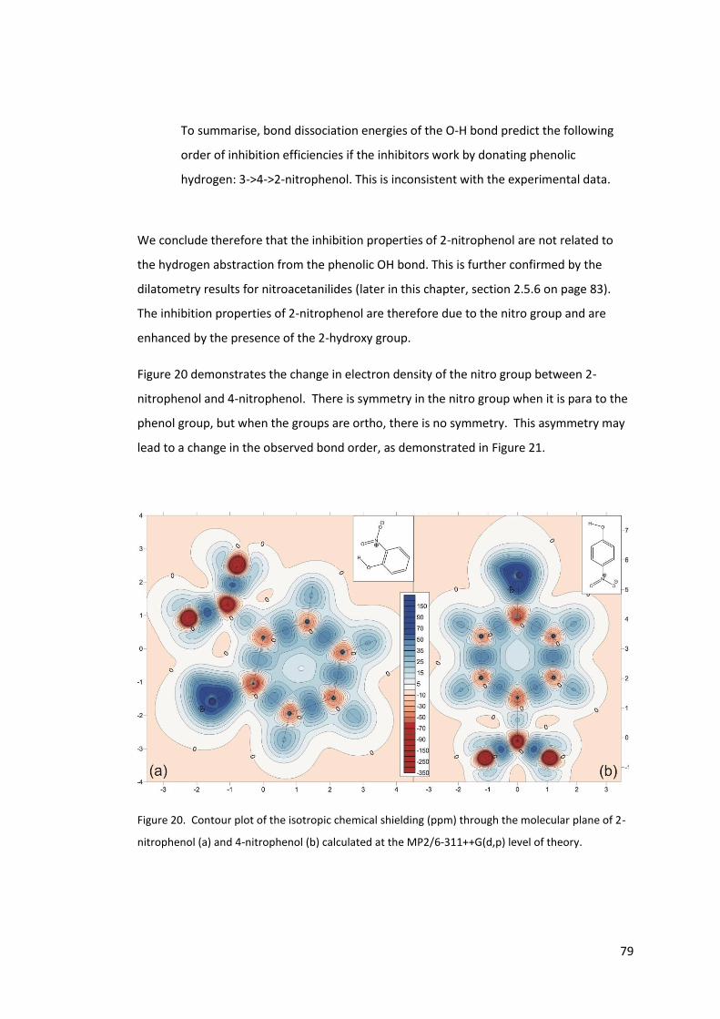
79
To summarise, bond dissociation energies of the O-H bond predict the following
order of inhibition efficiencies if the inhibitors work by donating phenolic
hydrogen: 3->4->2-nitrophenol. This is inconsistent with the experimental data.
We conclude therefore that the inhibition properties of 2-nitrophenol are not related to
the hydrogen abstraction from the phenolic OH bond. This is further confirmed by the
dilatometry results for nitroacetanilides (later in this chapter, section 2.5.6 on page 83).
The inhibition properties of 2-nitrophenol are therefore due to the nitro group and are
enhanced by the presence of the 2-hydroxy group.
Figure 20 demonstrates the change in electron density of the nitro group between 2-
nitrophenol and 4-nitrophenol. There is symmetry in the nitro group when it is para to the
phenol group, but when the groups are ortho, there is no symmetry. This asymmetry may
lead to a change in the observed bond order, as demonstrated in Figure 21.
Figure 20. Contour plot of the isotropic chemical shielding (ppm) through the molecular plane of 2-
nitrophenol (a) and 4-nitrophenol (b) calculated at the MP2/6-311++G(d,p) level of theory.
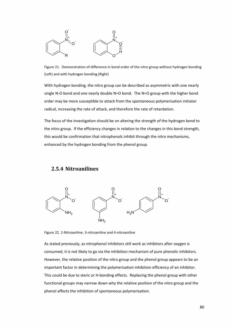
80
N+
O-
O
OH
N+
O-
R
O-
Figure 21. Demonstration of difference in bond order of the nitro group without hydrogen bonding
(Left) and with hydrogen bonding (Right)
With hydrogen bonding, the nitro group can be described as asymmetric with one nearly
single N-O bond and one nearly double N=O bond. The N=O group with the higher bond
order may be more susceptible to attack from the spontaneous polymerisation initiator
radical, increasing the rate of attack, and therefore the rate of retardation.
The focus of the investigation should be on altering the strength of the hydrogen bond to
the nitro group. If the efficiency changes in relation to the changes in this bond strength,
this would be confirmation that nitrophenols inhibit through the nitro mechanisms,
enhanced by the hydrogen bonding from the phenol group.
2.5.4 Nitroanilines
N+
O-
O
NH2
N+
O-
O
NH2
N+
O-
O
NH2
Figure 22. 2-Nitroaniline, 3-nitroaniline and 4-nitroaniline
As stated previously, as nitrophenol inhibitors still work as inhibitors after oxygen is
consumed, it is not likely to go via the inhibition mechanism of pure phenolic inhibitors.
However, the relative position of the nitro group and the phenol group appears to be an
important factor in determining the polymerisation inhibition efficiency of an inhibitor.
This could be due to steric or H-bonding effects. Replacing the phenol group with other
functional groups may narrow down why the relative position of the nitro group and the
phenol affects the inhibition of spontaneous polymerisation.
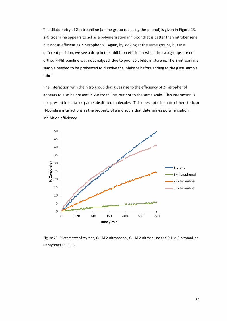
81
The dilatometry of 2-nitroaniline (amine group replacing the phenol) is given in Figure 23.
2-Nitroaniline appears to act as a polymerisation inhibitor that is better than nitrobenzene,
but not as efficient as 2-nitrophenol. Again, by looking at the same groups, but in a
different position, we see a drop in the inhibition efficiency when the two groups are not
ortho. 4-Nitroaniline was not analysed, due to poor solubility in styrene. The 3-nitroaniline
sample needed to be preheated to dissolve the inhibitor before adding to the glass sample
tube.
The interaction with the nitro group that gives rise to the efficiency of 2-nitrophenol
appears to also be present in 2-nitroaniline, but not to the same scale. This interaction is
not present in meta- or para-substituted molecules. This does not eliminate either steric or
H-bonding interactions as the property of a molecule that determines polymerisation
inhibition efficiency.
Figure 23 Dilatometry of styrene, 0.1 M 2-nitrophenol, 0.1 M 2-nitroaniline and 0.1 M 3-nitroaniline
(in styrene) at 110 °C.
0
5
10
15
20
25
30
35
40
45
50
0 120 240 360 480 600 720
% C
on
vers
ion
Time / min
Styrene
2 -nitrophenol
2-nitroaniline
3-nitroaniline
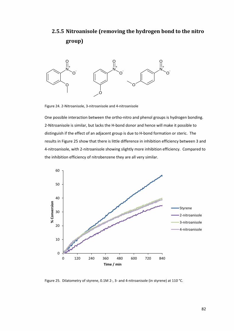
82
2.5.5 Nitroanisole (removing the hydrogen bond to the nitro
group)
N+
O-
O
O
N+
O-
O
O
N+
O-
O
O
Figure 24. 2-Nitroanisole, 3-nitroanisole and 4-nitroanisole
One possible interaction between the ortho-nitro and phenol groups is hydrogen bonding.
2-Nitroanisole is similar, but lacks the H-bond donor and hence will make it possible to
distinguish if the effect of an adjacent group is due to H-bond formation or steric. The
results in Figure 25 show that there is little difference in inhibition efficiency between 3 and
4-nitroanisole, with 2-nitroanisole showing slightly more inhibition efficiency. Compared to
the inhibition efficiency of nitrobenzene they are all very similar.
Figure 25. Dilatometry of styrene, 0.1M 2-, 3- and 4-nitroanisole (in styrene) at 110 °C.
0
10
20
30
40
50
60
0 120 240 360 480 600 720 840
% C
on
vers
ion
Time / min
Styrene
2-nitroanisole
3-nitroanisole
4-nitroanisole
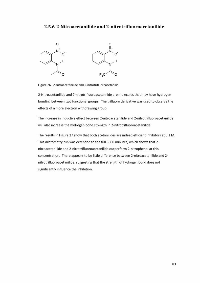
83
2.5.6 2-Nitroacetanilide and 2-nitrotrifluoroacetanilide
N+
O-
O
NH
O
N+
O-
O
NH
F3C O
Figure 26. 2-Nitroacetanilide and 2-nitrotrifluoroacetanilid
2-Nitroacetanilide and 2-nitrotrifluoroacetanilide are molecules that may have hydrogen
bonding between two functional groups. The trifluoro derivative was used to observe the
effects of a more electron withdrawing group.
The increase in inductive effect between 2-nitroacetanilide and 2-nitrotrifluoroacetanilide
will also increase the hydrogen bond strength in 2-nitrotrifluoroacetanilide.
The results in Figure 27 show that both acetanilides are indeed efficient inhibitors at 0.1 M.
This dilatometry run was extended to the full 3600 minutes, which shows that 2-
nitroacetanilide and 2-nitrotrifluoroacetanilide outperform 2-nitrophenol at this
concentration. There appears to be little difference between 2-nitroacetanilide and 2-
nitrotrifluoroacetanilide, suggesting that the strength of hydrogen bond does not
significantly influence the inhibition.
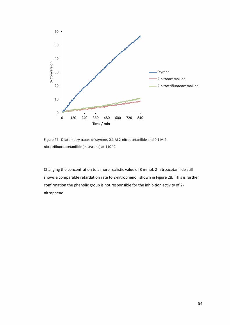
84
Figure 27. Dilatometry traces of styrene, 0.1 M 2-nitroacetanilide and 0.1 M 2-
nitrotrifluoroacetanilide (in styrene) at 110 °C.
Changing the concentration to a more realistic value of 3 mmol, 2-nitroacetanilide still
shows a comparable retardation rate to 2-nitrophenol, shown in Figure 28. This is further
confirmation the phenolic group is not responsible for the inhibition activity of 2-
nitrophenol.
0
10
20
30
40
50
60
0 120 240 360 480 600 720 840
% C
on
vers
ion
Time / min
Styrene
2-nitroacetanilide
2-nitrotrifluoroacetanilide
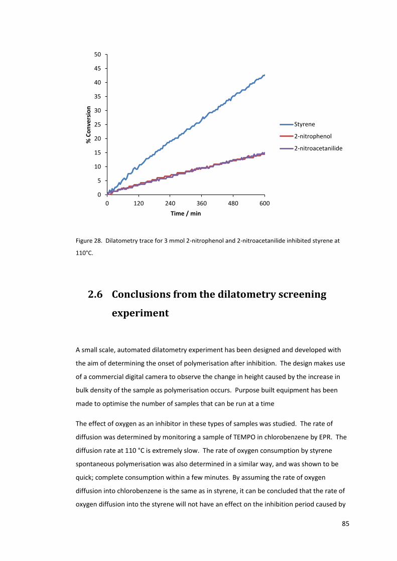
85
Figure 28. Dilatometry trace for 3 mmol 2-nitrophenol and 2-nitroacetanilide inhibited styrene at
110°C.
2.6 Conclusions from the dilatometry screening
experiment
A small scale, automated dilatometry experiment has been designed and developed with
the aim of determining the onset of polymerisation after inhibition. The design makes use
of a commercial digital camera to observe the change in height caused by the increase in
bulk density of the sample as polymerisation occurs. Purpose built equipment has been
made to optimise the number of samples that can be run at a time
The effect of oxygen as an inhibitor in these types of samples was studied. The rate of
diffusion was determined by monitoring a sample of TEMPO in chlorobenzene by EPR. The
diffusion rate at 110 °C is extremely slow. The rate of oxygen consumption by styrene
spontaneous polymerisation was also determined in a similar way, and was shown to be
quick; complete consumption within a few minutes. By assuming the rate of oxygen
diffusion into chlorobenzene is the same as in styrene, it can be concluded that the rate of
oxygen diffusion into the styrene will not have an effect on the inhibition period caused by
0
5
10
15
20
25
30
35
40
45
50
0 120 240 360 480 600
% C
on
vers
ion
Time / min
Styrene
2-nitrophenol
2-nitroacetanilide
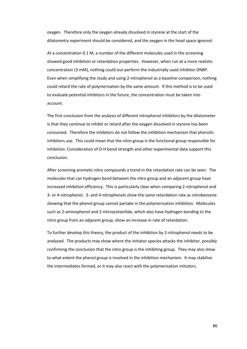
86
oxygen. Therefore only the oxygen already dissolved in styrene at the start of the
dilatometry experiment should be considered, and the oxygen in the head space ignored.
At a concentration 0.1 M, a number of the different molecules used in the screening
showed good inhibition or retardation properties. However, when run at a more realistic
concentration (3 mM), nothing could out-perform the industrially used inhibitor DNBP.
Even when simplifying the study and using 2-nitrophenol as a baseline comparison, nothing
could retard the rate of polymerisation by the same amount. If this method is to be used
to evaluate potential inhibitors in the future, the concentration must be taken into
account.
The first conclusion from the analysis of different nitrophenol inhibitors by the dilatometer
is that they continue to inhibit or retard after the oxygen dissolved in styrene has been
consumed. Therefore the inhibitors do not follow the inhibition mechanism that phenolic
inhibitors use. This could mean that the nitro group is the functional group responsible for
inhibition. Consideration of O-H bond strength and other experimental data support this
conclusion.
After screening aromatic nitro compounds a trend in the retardation rate can be seen. The
molecules that can hydrogen bond between the nitro group and an adjacent group have
increased inhibition efficiency. This is particularly clear when comparing 2-nitrophenol and
3- or 4-nitrophenol. 3- and 4-nitrophenols show the same retardation rate as nitrobenzene
showing that the phenol group cannot partake in the polymerisation inhibition. Molecules
such as 2-aminophenol and 2-nitroacetanilide, which also have hydrogen bonding to the
nitro group from an adjacent group, show an increase in rate of retardation.
To further develop this theory, the product of the inhibition by 2-nitrophenol needs to be
analysed. The products may show where the initiator species attacks the inhibitor, possibly
confirming the conclusion that the nitro group is the inhibiting group. They may also show
to what extent the phenol group is involved in the inhibition mechanism. It may stabilise
the intermediates formed, or it may also react with the polymerisation initiators.
87
3. Nitrophenols as inhibitors – Product analysis
3.1 Introduction
The products of styrene spontaneous polymerisation inhibition by nitrophenols, such as
DNBP, are not known. In a similar way to the dilatometry analysis, identifying the products
from the inhibition by a simpler related molecule, such as 2-nitrophenol, may allow easier
analysis of the inhibition mixture.
The concentrations of inhibitors used in industrial and commercial applications are low,
ranging from ~10-750 ppm. This means any intermediates and products will also be in
lower concentrations, depending on the mechanism. Therefore in this study, the
concentrations of the inhibitors will be increased, as to allow usable and identifiable
amounts of intermediates and / or products to be obtained.
In a paper, investigating a similar system to this, Bushby et al45 proposed the reaction in
Scheme 27. They used tert-butyl peroxide, a radical initiator, to form benzyl radicals from
toluene. DNBP reacts with this in the same way as it would with a polymerisation initiator.
They isolated the product 7-sec-butyl-5-nitro-2-phenolbenzoxazole from the reaction
mixture.
They suggest the reaction follows the mechanism proposed by Jackson and Waters46,
where the nitro group is reduced to an amine group. From there, the two products from
this reduction, (Amine A and aldehyde A in Scheme 27) react to form the
dihydrobenzoxazole. This is then oxidised to the benzoxazole isolated. They suggest this
route is the simplest of the possible mechanisms, but they do not discuss what the
alternatives are. Their separation method may be adapted to isolate the products from a
sample of inhibited styrene that has been heated to spontaneously polymerise.
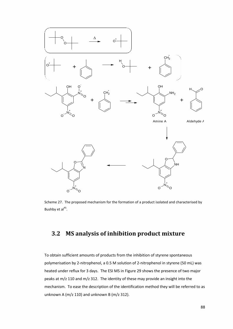
88
OH
N+
N+
O-
O
O
O-
CH2
OH
NH2
N+
O-
O
OH
O
NH
N+
O-
O
O
N
N+
O-
O
O
O O
O O
HCH2
+ +
+ +
Amine A Aldehyde A
Scheme 27. The proposed mechanism for the formation of a product isolated and characterised by
Bushby et al45
.
3.2 MS analysis of inhibition product mixture
To obtain sufficient amounts of products from the inhibition of styrene spontaneous
polymerisation by 2-nitrophenol, a 0.5 M solution of 2-nitrophenol in styrene (50 mL) was
heated under reflux for 3 days. The ESI MS in Figure 29 shows the presence of two major
peaks at m/z 110 and m/z 312. The identity of these may provide an insight into the
mechanism. To ease the description of the identification method they will be referred to as
unknown A (m/z 110) and unknown B (m/z 312).
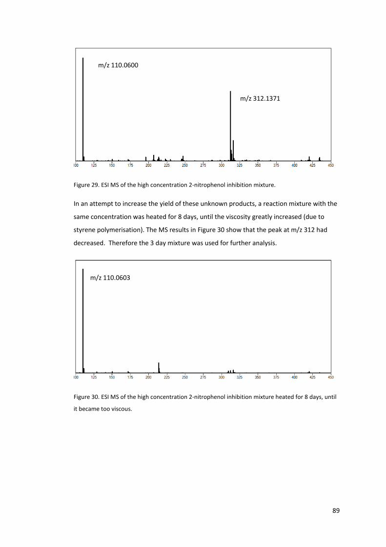
89
Figure 29. ESI MS of the high concentration 2-nitrophenol inhibition mixture.
In an attempt to increase the yield of these unknown products, a reaction mixture with the
same concentration was heated for 8 days, until the viscosity greatly increased (due to
styrene polymerisation). The MS results in Figure 30 show that the peak at m/z 312 had
decreased. Therefore the 3 day mixture was used for further analysis.
Figure 30. ESI MS of the high concentration 2-nitrophenol inhibition mixture heated for 8 days, until
it became too viscous.
m/z 312.1371
m/z 110.0600
m/z 110.0603
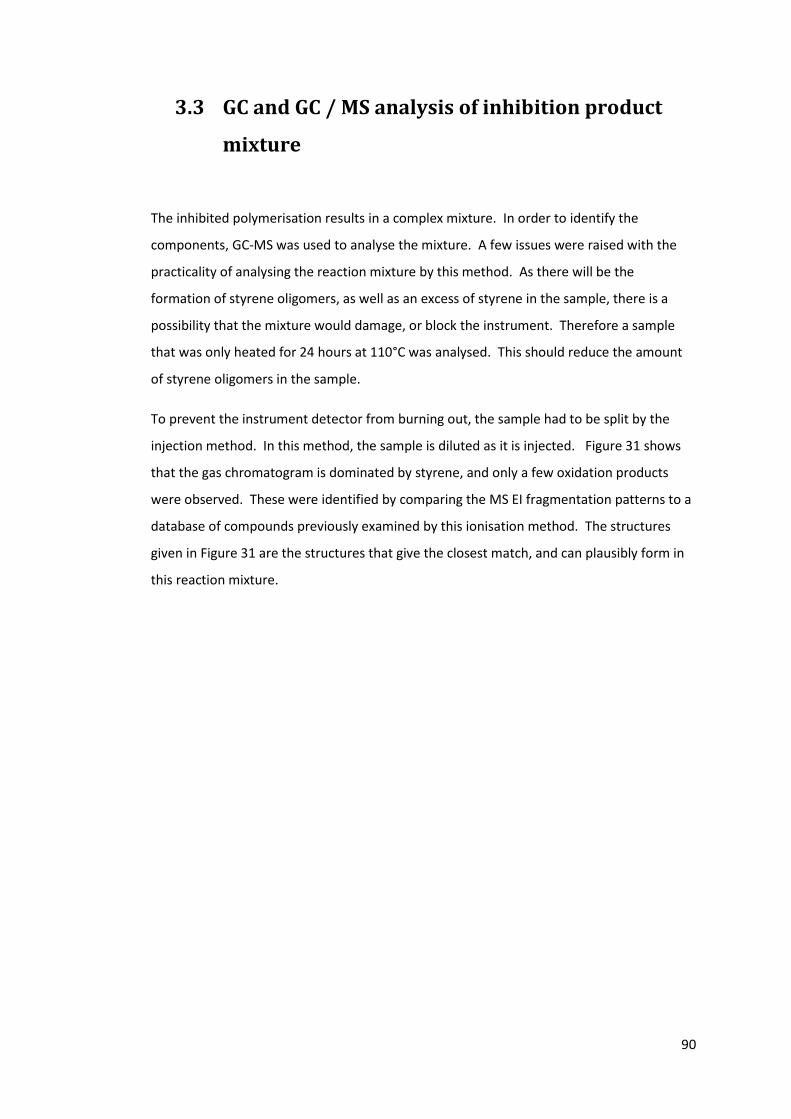
90
3.3 GC and GC / MS analysis of inhibition product
mixture
The inhibited polymerisation results in a complex mixture. In order to identify the
components, GC-MS was used to analyse the mixture. A few issues were raised with the
practicality of analysing the reaction mixture by this method. As there will be the
formation of styrene oligomers, as well as an excess of styrene in the sample, there is a
possibility that the mixture would damage, or block the instrument. Therefore a sample
that was only heated for 24 hours at 110°C was analysed. This should reduce the amount
of styrene oligomers in the sample.
To prevent the instrument detector from burning out, the sample had to be split by the
injection method. In this method, the sample is diluted as it is injected. Figure 31 shows
that the gas chromatogram is dominated by styrene, and only a few oxidation products
were observed. These were identified by comparing the MS EI fragmentation patterns to a
database of compounds previously examined by this ionisation method. The structures
given in Figure 31 are the structures that give the closest match, and can plausibly form in
this reaction mixture.
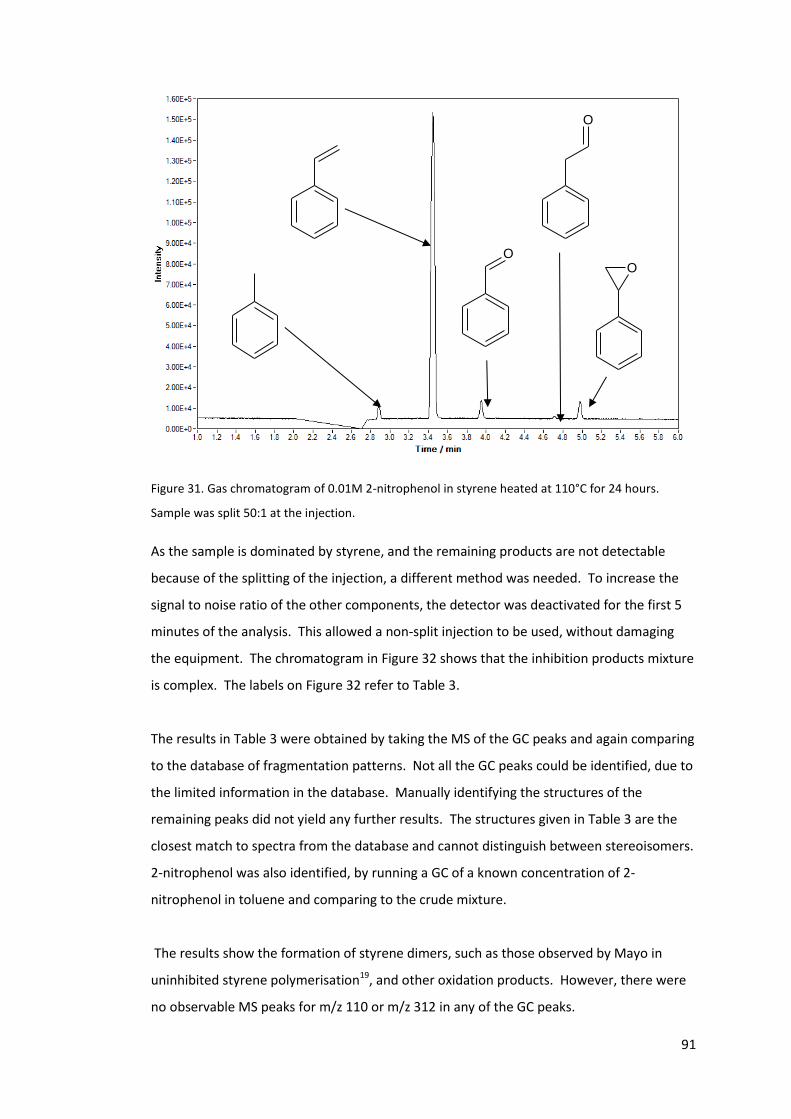
91
Figure 31. Gas chromatogram of 0.01M 2-nitrophenol in styrene heated at 110°C for 24 hours.
Sample was split 50:1 at the injection.
As the sample is dominated by styrene, and the remaining products are not detectable
because of the splitting of the injection, a different method was needed. To increase the
signal to noise ratio of the other components, the detector was deactivated for the first 5
minutes of the analysis. This allowed a non-split injection to be used, without damaging
the equipment. The chromatogram in Figure 32 shows that the inhibition products mixture
is complex. The labels on Figure 32 refer to Table 3.
The results in Table 3 were obtained by taking the MS of the GC peaks and again comparing
to the database of fragmentation patterns. Not all the GC peaks could be identified, due to
the limited information in the database. Manually identifying the structures of the
remaining peaks did not yield any further results. The structures given in Table 3 are the
closest match to spectra from the database and cannot distinguish between stereoisomers.
2-nitrophenol was also identified, by running a GC of a known concentration of 2-
nitrophenol in toluene and comparing to the crude mixture.
The results show the formation of styrene dimers, such as those observed by Mayo in
uninhibited styrene polymerisation19, and other oxidation products. However, there were
no observable MS peaks for m/z 110 or m/z 312 in any of the GC peaks.
O
O
O
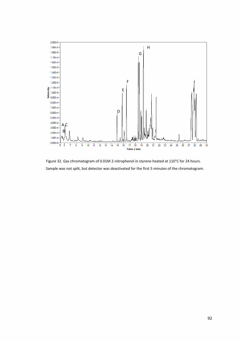
92
Figure 32. Gas chromatogram of 0.01M 2-nitrophenol in styrene heated at 110°C for 24 hours.
Sample was not split, but detector was deactivated for the first 5 minutes of the chromatogram.
A C
B
D
E
F
G
H
J
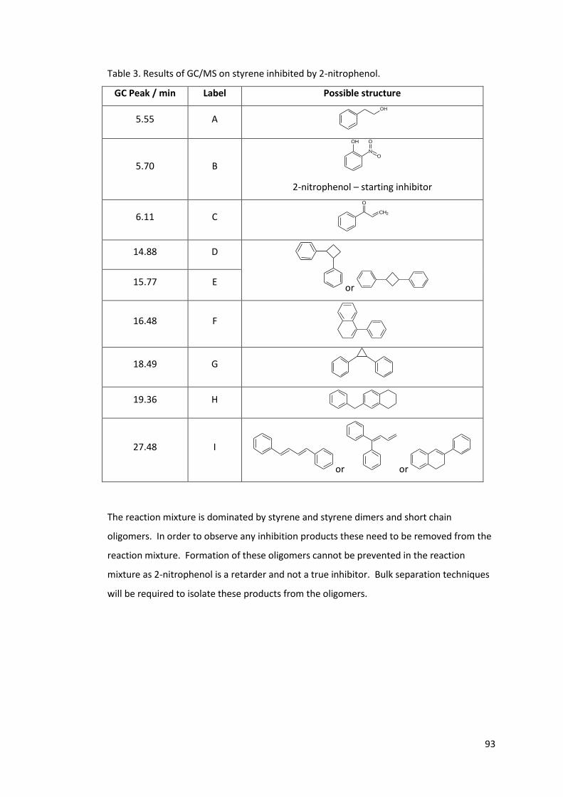
93
Table 3. Results of GC/MS on styrene inhibited by 2-nitrophenol.
GC Peak / min Label Possible structure
5.55 A OH
5.70 B
N
OH
O
O
2-nitrophenol – starting inhibitor
6.11 C CH2
O
14.88 D
or 15.77 E
16.48 F
18.49 G
19.36 H
27.48 I
or or
The reaction mixture is dominated by styrene and styrene dimers and short chain
oligomers. In order to observe any inhibition products these need to be removed from the
reaction mixture. Formation of these oligomers cannot be prevented in the reaction
mixture as 2-nitrophenol is a retarder and not a true inhibitor. Bulk separation techniques
will be required to isolate these products from the oligomers.

94
3.4 Identification of reactive intermediates by EPR
Previous studies have shown that propagating radicals will react with nitro groups to form
nitroxides as intermediates in the reaction. Bartlett at al94 specifically looked at the
polymerisation of vinyl acetate inhibited by nitro compounds. EPR spectroscopy should be
able to observe any long lived nitroxide radicals form by the inhibition of spontaneous
polymerisation.
Also, it has been established that TEMPO is an efficient polymerisation inhibitor95. If a
nitroxide is formed from the reaction between radical initiator and inhibitor, it may be that
the nitroxide is the inhibiting species rather than a nitro group itself. Similarly, as observed
in the previous chapter, the interaction between the nitroxide and the phenol group may
also play a part in the inhibition efficiency of ortho nitrophenols
The reaction in Scheme 28 shows the formation of an alkoxynitroxide intermediate,
followed by fragmentation to give a nitroso compound. Scheme 29 shows an alternative
fragmentation of alkoxynitroxide leading to the formation of nitroso compound, aldehyde
and an alkane. Jackson and Waters46 proposed this mechanism as they observed the
formation of aldehyde in the experiments.
N+
O-
O
RN
O
O
R R N
O
R O
R+
Scheme 28. Formation of nitroso arene as proposed by Bartlett et al94
, via a nitroxide intermediate.
Motyakin et al49 recorded the EPR spectra for the nitroxide formed from nitro and nitroso
containing inhibitors. Nitroso compounds can form dialkyl nitroxide radicals when they
react with the carbon-centred radicals formed and the authors proposed that the observed
radical is the alkyl aryl nitroxide formed from the nitroso compound (See Scheme 30). This
also matches the hyperfine splitting from the EPR spectra.
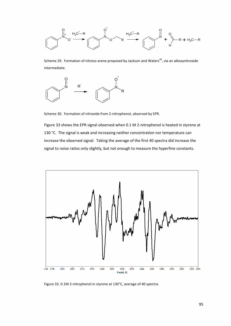
95
N+
O-
O
NO
O
R
CH2 R CH2 RN
O
R
O
H
+ CH3 R+
Scheme 29. Formation of nitroso arene proposed by Jackson and Waters46
, via an alkoxynitroxide
intermediate.
N
O
R N
O
R
Scheme 30. Formation of nitroxide from 2-nitrophenol, observed by EPR.
Figure 33 shows the EPR signal observed when 0.1 M 2-nitrophenol is heated in styrene at
130 °C. The signal is weak and increasing neither concentration nor temperature can
increase the observed signal. Taking the average of the first 40 spectra did increase the
signal to noise ratios only slightly, but not enough to measure the hyperfine constants.
Figure 33. 0.1M 2-nitrophenol in styrene at 130°C, average of 40 spectra.
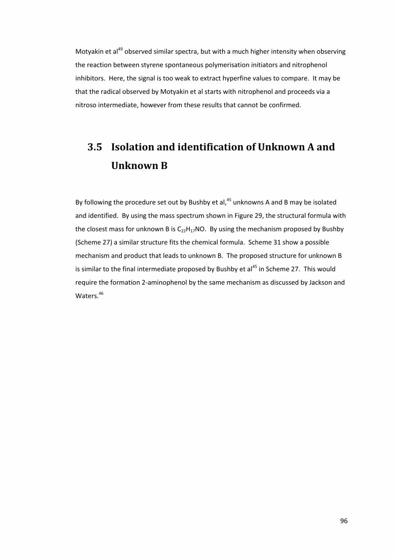
96
Motyakin et al49 observed similar spectra, but with a much higher intensity when observing
the reaction between styrene spontaneous polymerisation initiators and nitrophenol
inhibitors. Here, the signal is too weak to extract hyperfine values to compare. It may be
that the radical observed by Motyakin et al starts with nitrophenol and proceeds via a
nitroso intermediate, however from these results that cannot be confirmed.
3.5 Isolation and identification of Unknown A and
Unknown B
By following the procedure set out by Bushby et al,45 unknowns A and B may be isolated
and identified. By using the mass spectrum shown in Figure 29, the structural formula with
the closest mass for unknown B is C22H17NO. By using the mechanism proposed by Bushby
(Scheme 27) a similar structure fits the chemical formula. Scheme 31 show a possible
mechanism and product that leads to unknown B. The proposed structure for unknown B
is similar to the final intermediate proposed by Bushby et al45 in Scheme 27. This would
require the formation 2-aminophenol by the same mechanism as discussed by Jackson and
Waters.46

97
N+
O-
OOH
NH2
OH
CH
NH
O+
H
Unknown Intermediate
Jackson and Water's mechanism
Scheme 31. Proposed formation of Unknown B following previous research by Jackson and
Waters46
, and by Bushby et al45
.
3.5.1 Acid / Base extraction
To split the polymerisation inhibition mixture into smaller, less complex samples, it was
dissolved in diethyl ether (50 mL) and then washed with aqueous acid (5 M HCl) and base
(5 M NaOH) to isolate compounds with different acidic or basic groups. Normally the
aqueous acidic or basic washes are neutralised and extracted with an organic or
halogenated solvent. This however yielded nothing observable by NMR or MS.
Figure 34 shows the ESI of the acid extract and the remaining neutral organic layer. This
shows that unknown A has been removed from the product mixture, leaving unknown B in
the neutral organic solution. The neutral organic fraction yield after removal of solvent was
1.88 g from an input of 5 g crude; this suggests that a significant amount of material was
extracted during washes.
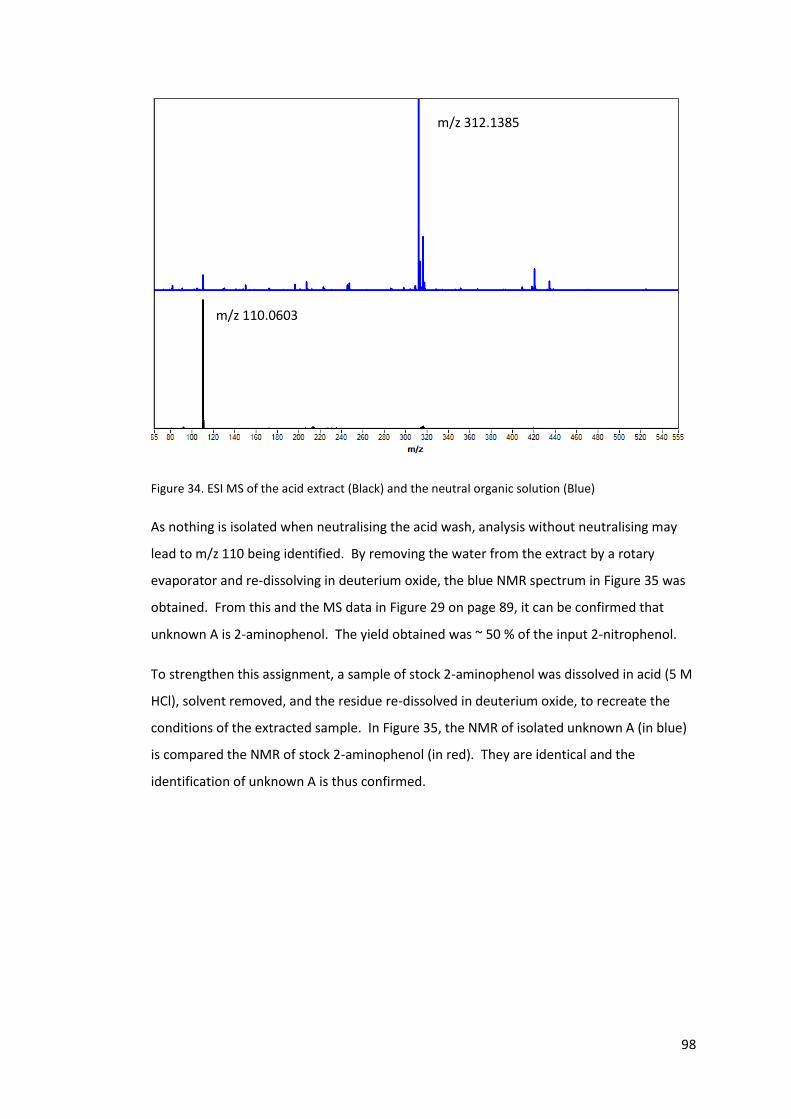
98
Figure 34. ESI MS of the acid extract (Black) and the neutral organic solution (Blue)
As nothing is isolated when neutralising the acid wash, analysis without neutralising may
lead to m/z 110 being identified. By removing the water from the extract by a rotary
evaporator and re-dissolving in deuterium oxide, the blue NMR spectrum in Figure 35 was
obtained. From this and the MS data in Figure 29 on page 89, it can be confirmed that
unknown A is 2-aminophenol. The yield obtained was ~ 50 % of the input 2-nitrophenol.
To strengthen this assignment, a sample of stock 2-aminophenol was dissolved in acid (5 M
HCl), solvent removed, and the residue re-dissolved in deuterium oxide, to recreate the
conditions of the extracted sample. In Figure 35, the NMR of isolated unknown A (in blue)
is compared the NMR of stock 2-aminophenol (in red). They are identical and the
identification of unknown A is thus confirmed.
m/z 110.0603
m/z 312.1385
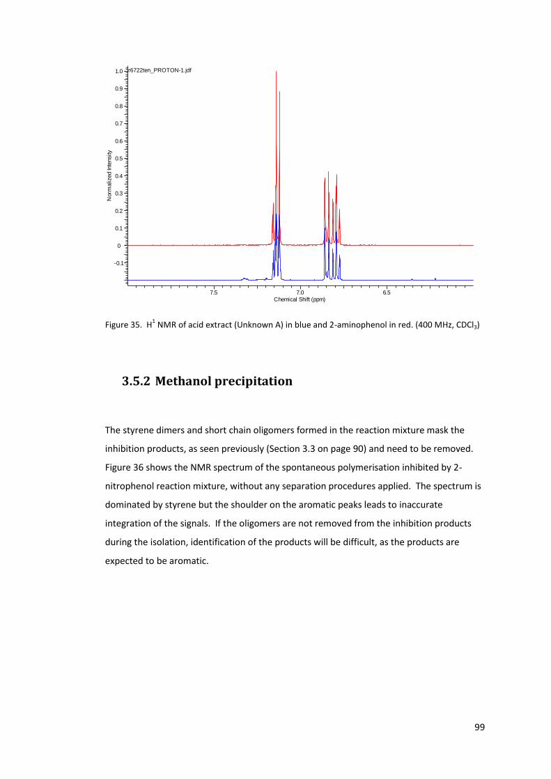
99
r6722ten_PROTON-1.jdf
7.5 7.0 6.5
Chemical Shift (ppm)
-0.1
0
0.1
0.2
0.3
0.4
0.5
0.6
0.7
0.8
0.9
1.0
Norm
alized Inte
nsity
Figure 35. H1 NMR of acid extract (Unknown A) in blue and 2-aminophenol in red. (400 MHz, CDCl3)
3.5.2 Methanol precipitation
The styrene dimers and short chain oligomers formed in the reaction mixture mask the
inhibition products, as seen previously (Section 3.3 on page 90) and need to be removed.
Figure 36 shows the NMR spectrum of the spontaneous polymerisation inhibited by 2-
nitrophenol reaction mixture, without any separation procedures applied. The spectrum is
dominated by styrene but the shoulder on the aromatic peaks leads to inaccurate
integration of the signals. If the oligomers are not removed from the inhibition products
during the isolation, identification of the products will be difficult, as the products are
expected to be aromatic.

100
K3.esp
8.5 8.0 7.5 7.0 6.5 6.0 5.5 5.0 4.5 4.0 3.5 3.0 2.5 2.0 1.5 1.0
Chemical Shift (ppm)
0.1
0.2
0.3
0.4
0.5
0.6
0.7
0.8
0.9
1.0
Norm
alized Inte
nsity
Figure 36. H1 NMR of reaction mixture without any separation. (400 MHz, CDCl3)
The longer polystyrene chains were therefore precipitated out by methanol. A slurry was
obtained by adding the neutral fraction from the acid / base extraction to methanol. This
was then cooled in a freezer for at least 2 hours then filtered through celite.
The precipitate obtained was not white as is expected for pure polystyrene, but was dark
brown. This suggests there will be other inhibition products in the precipitate. Additional
washes do not improve the yield of the methanol wash residue.
The methanol was removed by rotary evaporation. This also removes any excess styrene
and other volatile compounds from the mixture.
3.5.3 Column chromatography
The next stage of separation was by column chromatography, monitored by TLC. The
isolation of unknown B took longer than anticipated due to a number of factors that
increased the difficulty of the isolation, such as its decomposition observed once isolated.
The dominance and persistence of the polystyrene oligomers made identification of the
compound after isolation difficult. The chromatography was performed as reported by Still
et al96, with further alterations, as described later. Through the use of different solvent
Styrene
Styrene
2-nitrophenol
Hump in base line
due to polystyrene
Shoulder on
aromatic
peaks due to
polystyrene

101
systems the separation of unknown B was obtained. The optimised procedure used two
successive separations in different solvent systems: diethyl ether and 1:1 DCM : hexane.
This was after many attempts, due to the poor stability of unknown B in neat form and due
to the issues caused by polystyrene any other styrene oligomers remaining. The procedure
given below is the final and most successful procedure developed.
A TLC using diethyl ether shows two main components, with Rf values of ~0.5 and ~0. The
spots at Rf 0.5 contained unknown B, as observed by MS. When evaluating the different
systems, it was noticed that performing this separation first, allows the following samples
to be separated easier, i.e. there is less streaking of the fractions visible on TLC plates.
The solvent system for the next separation was 1:1 DCM : hexane. Although similar
separation can be achieved by other solvent systems, the reaction mixture is most soluble
in this solvent system. This facilitates separation of larger samples.
Figure 37 is the MS of a fraction obtained from the mixture (Rf = 0.33 in 1:1 DCM: hexane,
72 mg collected). A strong peak with m/z 312 dominates the spectrum. The NMR of the
fraction (Figure 38) shows that the sample is not pure, and the broad peaks from the
impurities suggest that there are still short chain polystyrene oligomers present. These
oligomers are soluble in methanol and are not volatile enough to be removed by vacuum
distillation.
Figure 37. MS of fraction containing unknown B (Rf = 0.33).
m/z 312.1382
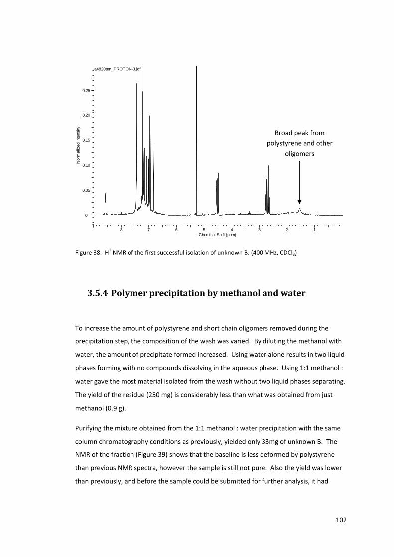
102
a4820ten_PROTON-3.jdf
8 7 6 5 4 3 2 1
Chemical Shift (ppm)
0
0.05
0.10
0.15
0.20
0.25
Norm
alized Inte
nsity
Figure 38. H1 NMR of the first successful isolation of unknown B. (400 MHz, CDCl3)
3.5.4 Polymer precipitation by methanol and water
To increase the amount of polystyrene and short chain oligomers removed during the
precipitation step, the composition of the wash was varied. By diluting the methanol with
water, the amount of precipitate formed increased. Using water alone results in two liquid
phases forming with no compounds dissolving in the aqueous phase. Using 1:1 methanol :
water gave the most material isolated from the wash without two liquid phases separating.
The yield of the residue (250 mg) is considerably less than what was obtained from just
methanol (0.9 g).
Purifying the mixture obtained from the 1:1 methanol : water precipitation with the same
column chromatography conditions as previously, yielded only 33mg of unknown B. The
NMR of the fraction (Figure 39) shows that the baseline is less deformed by polystyrene
than previous NMR spectra, however the sample is still not pure. Also the yield was lower
than previously, and before the sample could be submitted for further analysis, it had
Broad peak from
polystyrene and other
oligomers
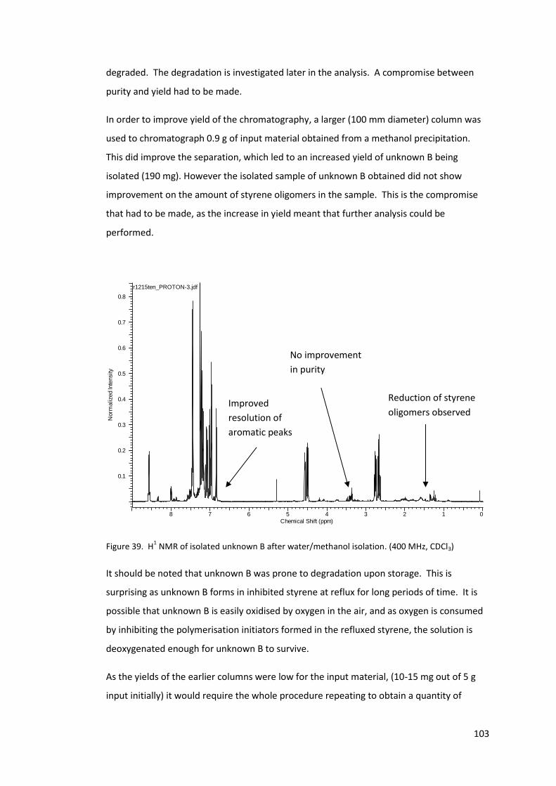
103
degraded. The degradation is investigated later in the analysis. A compromise between
purity and yield had to be made.
In order to improve yield of the chromatography, a larger (100 mm diameter) column was
used to chromatograph 0.9 g of input material obtained from a methanol precipitation.
This did improve the separation, which led to an increased yield of unknown B being
isolated (190 mg). However the isolated sample of unknown B obtained did not show
improvement on the amount of styrene oligomers in the sample. This is the compromise
that had to be made, as the increase in yield meant that further analysis could be
performed.
r1215ten_PROTON-3.jdf
8 7 6 5 4 3 2 1 0
Chemical Shift (ppm)
0.1
0.2
0.3
0.4
0.5
0.6
0.7
0.8
Norm
alized Inte
nsity
Figure 39. H1 NMR of isolated unknown B after water/methanol isolation. (400 MHz, CDCl3)
It should be noted that unknown B was prone to degradation upon storage. This is
surprising as unknown B forms in inhibited styrene at reflux for long periods of time. It is
possible that unknown B is easily oxidised by oxygen in the air, and as oxygen is consumed
by inhibiting the polymerisation initiators formed in the refluxed styrene, the solution is
deoxygenated enough for unknown B to survive.
As the yields of the earlier columns were low for the input material, (10-15 mg out of 5 g
input initially) it would require the whole procedure repeating to obtain a quantity of
Reduction of styrene
oligomers observed
No improvement
in purity
Improved
resolution of
aromatic peaks
104
unknown B to analyse before oxidation. A lot of time, energy and resources were thus
spent on this section of the study.
3.6 Structure determination of unknown B by NMR
The fraction containing unknown B was analysed by 1H NMR spectroscopy. The 400 MHz
spectrometer available does not provide sufficient resolution to distinguish all the proton
signals (see Figure 38 and Figure 39). Therefore, a 700 MHz spectrometer was used for
analysis and structure determination.
There are 9 unique proton signals, labelled in Figure 40 and Figure 41 from low to high
field. The integration of the peaks will be somewhat inaccurate due to the remaining
polystyrene in the sample, missed by the methanol precipitation step of the isolation.
However the total integration from the protons signals can be estimated at 17 in total.
The 13C NMR signals are labelled with a similar system in Figure 108, page 222 in the
appendix. This system is used in Table 5 and Table 6 below, and in Table 13 and Table 14 in
the appendix, show all the couplings determined from the homonuclear correlation
spectroscopy, heteronuclear single-quantum correlation spectroscopy and heteronuclear
multiple-bond correlation spectroscopy (COSY, HSQC and HMBC respectively) 2D NMR
experiments. The 2D spectra are given in the Appendix, starting page 216.
There are 20 carbon signals in the 13C spectra. By combining this data with the MS
information, the chemical formula could be C22H17NO. This would mean there are 2 carbon
environments that represent 2 carbons each.
Carbons 14 and 15 are so close in the spectrum, any couplings in the HMBC spectra cannot
be separated between the two. Proton B appears to represent 3 protons, but this may not
mean 3 of the same chemical environment. The splitting pattern and the number of
couplings in the 2D data suggest it is multiple chemical environments that have the same
chemical shift. This will make a complete assignment difficult.

105
Figure 40. 1H NMR of unkown B, low field. (700 MHz, CDCl3)
Figure 41. 1H NMR of unknown B, high field. (700 MHz, CDCl3)
I
H
G F
D E
C B
A
L M J K
105
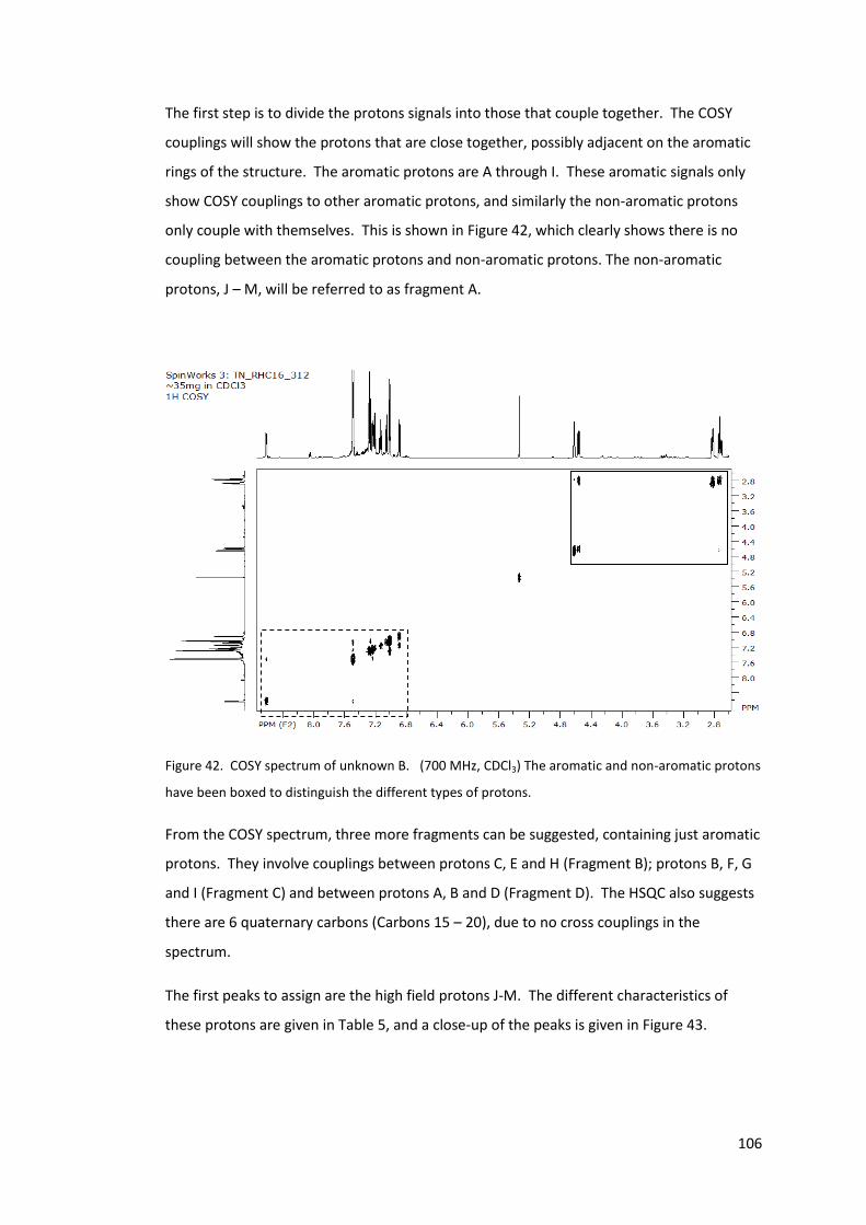
106
The first step is to divide the protons signals into those that couple together. The COSY
couplings will show the protons that are close together, possibly adjacent on the aromatic
rings of the structure. The aromatic protons are A through I. These aromatic signals only
show COSY couplings to other aromatic protons, and similarly the non-aromatic protons
only couple with themselves. This is shown in Figure 42, which clearly shows there is no
coupling between the aromatic protons and non-aromatic protons. The non-aromatic
protons, J – M, will be referred to as fragment A.
Figure 42. COSY spectrum of unknown B. (700 MHz, CDCl3) The aromatic and non-aromatic protons
have been boxed to distinguish the different types of protons.
From the COSY spectrum, three more fragments can be suggested, containing just aromatic
protons. They involve couplings between protons C, E and H (Fragment B); protons B, F, G
and I (Fragment C) and between protons A, B and D (Fragment D). The HSQC also suggests
there are 6 quaternary carbons (Carbons 15 – 20), due to no cross couplings in the
spectrum.
The first peaks to assign are the high field protons J-M. The different characteristics of
these protons are given in Table 5, and a close-up of the peaks is given in Figure 43.
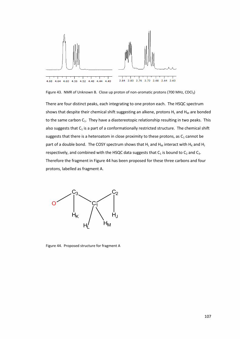
107
Figure 43. NMR of Unknown B. Close up proton of non-aromatic protons (700 MHz, CDCl3)
There are four distinct peaks, each integrating to one proton each. The HSQC spectrum
shows that despite their chemical shift suggesting an alkene, protons HL and HM are bonded
to the same carbon C1. They have a diastereotopic relationship resulting in two peaks. This
also suggests that C1 is a part of a conformationally restricted structure. The chemical shift
suggests that there is a heteroatom in close proximity to these protons, as C1 cannot be
part of a double bond. The COSY spectrum shows that HL and HM interact with HK and HJ
respectively, and combined with the HSQC data suggests that C1 is bound to C2 and C3.
Therefore the fragment in Figure 44 has been proposed for these three carbons and four
protons, labelled as fragment A.
Figure 44. Proposed structure for fragment A
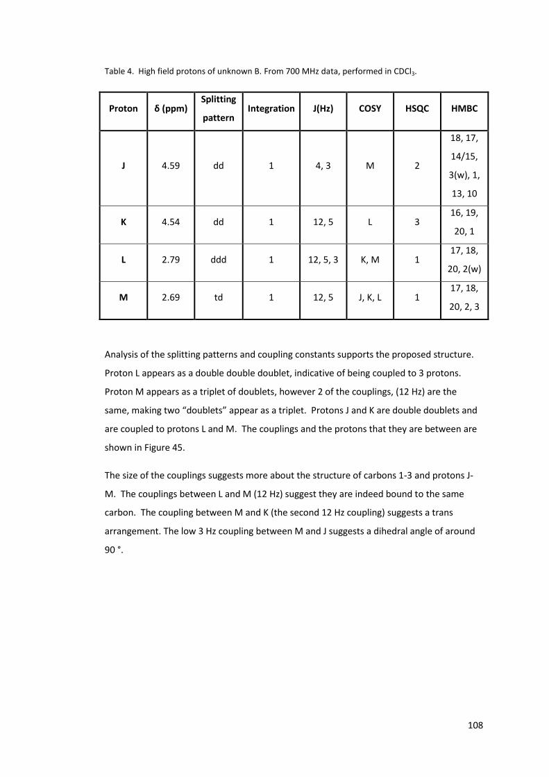
108
Table 4. High field protons of unknown B. From 700 MHz data, performed in CDCl3.
Proton δ (ppm) Splitting
pattern Integration J(Hz) COSY HSQC HMBC
J 4.59 dd 1 4, 3 M 2
18, 17,
14/15,
3(w), 1,
13, 10
K 4.54 dd 1 12, 5 L 3 16, 19,
20, 1
L 2.79 ddd 1 12, 5, 3 K, M 1 17, 18,
20, 2(w)
M 2.69 td 1 12, 5 J, K, L 1 17, 18,
20, 2, 3
Analysis of the splitting patterns and coupling constants supports the proposed structure.
Proton L appears as a double double doublet, indicative of being coupled to 3 protons.
Proton M appears as a triplet of doublets, however 2 of the couplings, (12 Hz) are the
same, making two “doublets” appear as a triplet. Protons J and K are double doublets and
are coupled to protons L and M. The couplings and the protons that they are between are
shown in Figure 45.
The size of the couplings suggests more about the structure of carbons 1-3 and protons J-
M. The couplings between L and M (12 Hz) suggest they are indeed bound to the same
carbon. The coupling between M and K (the second 12 Hz coupling) suggests a trans
arrangement. The low 3 Hz coupling between M and J suggests a dihedral angle of around
90 °.
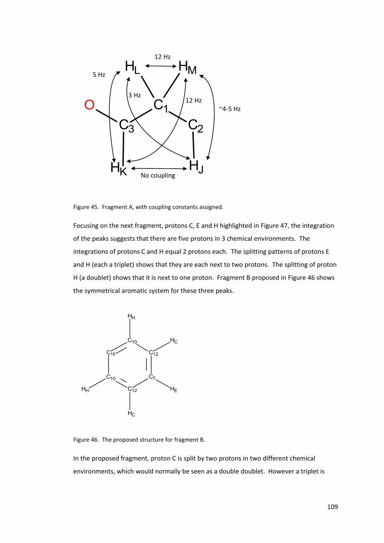
109
Figure 45. Fragment A, with coupling constants assigned.
Focusing on the next fragment, protons C, E and H highlighted in Figure 47, the integration
of the peaks suggests that there are five protons in 3 chemical environments. The
integrations of protons C and H equal 2 protons each. The splitting patterns of protons E
and H (each a triplet) shows that they are each next to two protons. The splitting of proton
H (a doublet) shows that it is next to one proton. Fragment B proposed in Figure 46 shows
the symmetrical aromatic system for these three peaks.
Figure 46. The proposed structure for fragment B.
In the proposed fragment, proton C is split by two protons in two different chemical
environments, which would normally be seen as a double doublet. However a triplet is
5 Hz
12 Hz
12 Hz ~4-5 Hz
No coupling
3 Hz
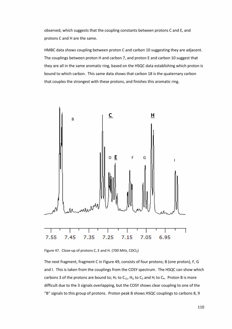
110
observed, which suggests that the coupling constants between protons C and E, and
protons C and H are the same.
HMBC data shows coupling between proton C and carbon 10 suggesting they are adjacent.
The couplings between proton H and carbon 7, and proton E and carbon 10 suggest that
they are all in the same aromatic ring, based on the HSQC data establishing which proton is
bound to which carbon. This same data shows that carbon 18 is the quaternary carbon
that couples the strongest with these protons, and finishes this aromatic ring.
Figure 47. Close-up of protons C, E and H. (700 MHz, CDCl3)
The next fragment, fragment C in Figure 49, consists of four protons; B (one proton), F, G
and I. This is taken from the couplings from the COSY spectrum. The HSQC can show which
carbons 3 of the protons are bound to; HF to C11, HG to C5 and HI to C4. Proton B is more
difficult due to the 3 signals overlapping, but the COSY shows clear coupling to one of the
“B” signals to this group of protons. Proton peak B shows HSQC couplings to carbons 8, 9
B C H
D E F G I

111
and 14. To determine which of these carbons belong to fragment C, the HMBC couplings to
protons F and G are used. The HMBC only shows coupling to protons F and G and carbon 8,
with no couplings to carbons 9 and 14. This means carbon 8 is somewhere near to protons
F and G, within fragment C. This suggests that the proton B signal from fragment C is
bound to carbon 8.
The order in which the protons are placed around the aromatic fragment can be
determined firstly be the splitting in the proton spectrum and then by the HMBC couplings.
Protons F and G are triplet of doublets, suggesting they are adjacent to two protons each.
Whereas proton I is a double doublet, suggesting it is adjacent to only one proton. As there
are HMBC couplings of the “inner“ protons F and G to proton B, the fragment in Figure 49 is
proposed.
Figure 48. Close-up of protons B, F, G and I. (700 MHz, CDCl3)
B C H
D E F G
I
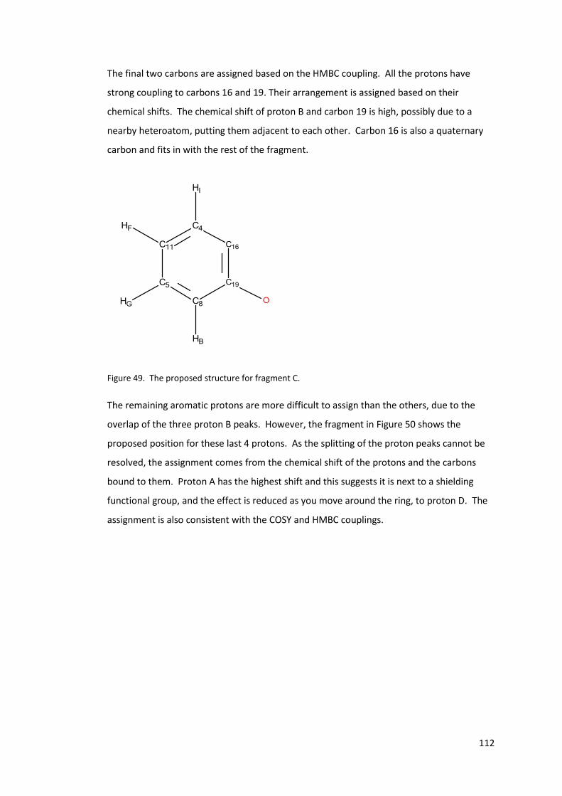
112
The final two carbons are assigned based on the HMBC coupling. All the protons have
strong coupling to carbons 16 and 19. Their arrangement is assigned based on their
chemical shifts. The chemical shift of proton B and carbon 19 is high, possibly due to a
nearby heteroatom, putting them adjacent to each other. Carbon 16 is also a quaternary
carbon and fits in with the rest of the fragment.
Figure 49. The proposed structure for fragment C.
The remaining aromatic protons are more difficult to assign than the others, due to the
overlap of the three proton B peaks. However, the fragment in Figure 50 shows the
proposed position for these last 4 protons. As the splitting of the proton peaks cannot be
resolved, the assignment comes from the chemical shift of the protons and the carbons
bound to them. Proton A has the highest shift and this suggests it is next to a shielding
functional group, and the effect is reduced as you move around the ring, to proton D. The
assignment is also consistent with the COSY and HMBC couplings.
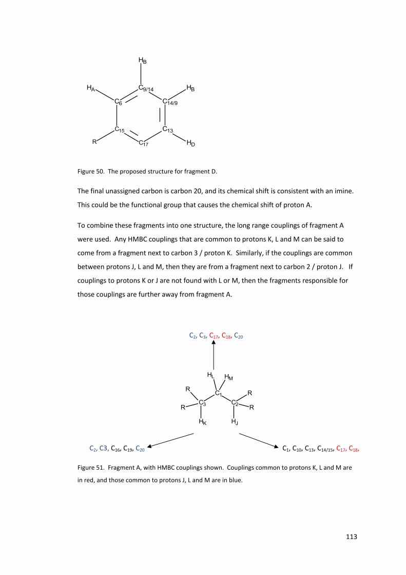
113
Figure 50. The proposed structure for fragment D.
The final unassigned carbon is carbon 20, and its chemical shift is consistent with an imine.
This could be the functional group that causes the chemical shift of proton A.
To combine these fragments into one structure, the long range couplings of fragment A
were used. Any HMBC couplings that are common to protons K, L and M can be said to
come from a fragment next to carbon 3 / proton K. Similarly, if the couplings are common
between protons J, L and M, then they are from a fragment next to carbon 2 / proton J. If
couplings to protons K or J are not found with L or M, then the fragments responsible for
those couplings are further away from fragment A.
Figure 51. Fragment A, with HMBC couplings shown. Couplings common to protons K, L and M are
in red, and those common to protons J, L and M are in blue.
C1, C10, C13, C14/15, C17, C18, C2, C3, C16, C19, C20
C2, C3, C17, C18, C20
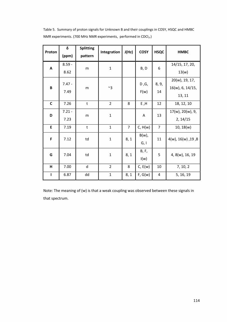
114
Table 5. Summary of proton signals for Unknown B and their couplings in COSY, HSQC and HMBC
NMR experiments. (700 MHz NMR experiments, performed in CDCl3.)
Proton δ
(ppm)
Splitting
pattern Integration J(Hz) COSY HSQC HMBC
A 8.59 -
8.62 m 1 B, D 6
14/15, 17, 20,
13(w)
B 7.47 -
7.49 m ~3
D ,G,
F(w)
8, 9,
14
20(w), 19, 17,
16(w), 6, 14/15,
13, 11
C 7.26 t 2 8 E ,H 12 18, 12, 10
D 7.21 -
7.23 m 1 A 13
17(w), 20(w), 9,
2, 14/15
E 7.19 t 1 7 C, H(w) 7 10, 18(w)
F 7.12 td 1 8, 1 B(w),
G, I 11 4(w), 16(w) ,19 ,8
G 7.04 td 1 8, 1 B, F,
I(w) 5 4, 8(w), 16, 19
H 7.00 d 2 8 C, E(w) 10 7, 10, 2
I 6.87 dd 1 8, 1 F, G(w) 4 5, 16, 19
Note: The meaning of (w) is that a weak coupling was observed between these signals in
that spectrum.
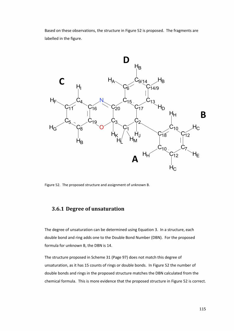
115
Based on these observations, the structure in Figure 52 is proposed. The fragments are
labelled in the figure.
Figure 52. The proposed structure and assignment of unknown B.
3.6.1 Degree of unsaturation
The degree of unsaturation can be determined using Equation 3. In a structure, each
double bond and ring adds one to the Double Bond Number (DBN). For the proposed
formula for unknown B, the DBN is 14.
The structure proposed in Scheme 31 (Page 97) does not match this degree of
unsaturation, as it has 15 counts of rings or double bonds. In Figure 52 the number of
double bonds and rings in the proposed structure matches the DBN calculated from the
chemical formula. This is more evidence that the proposed structure in Figure 52 is correct.
C
D
B
A
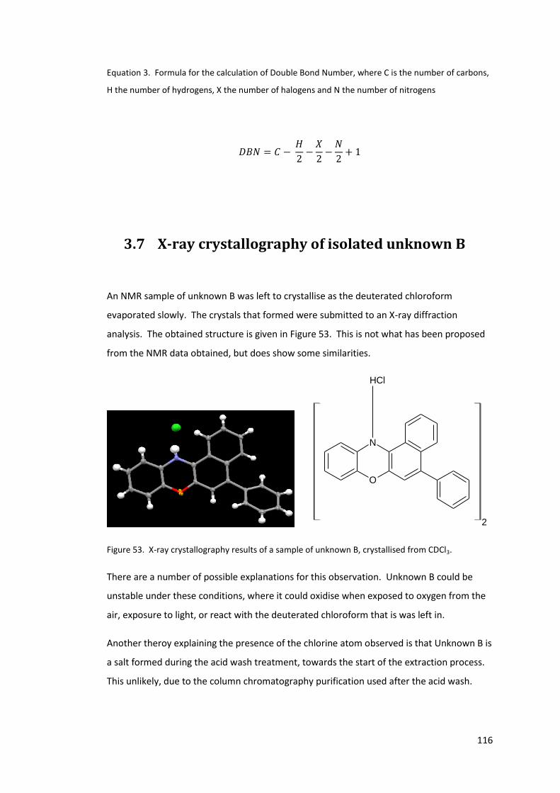
116
Equation 3. Formula for the calculation of Double Bond Number, where C is the number of carbons,
H the number of hydrogens, X the number of halogens and N the number of nitrogens
𝐷𝐵𝑁 = 𝐶 − 𝐻
2−𝑋
2−𝑁
2+ 1
3.7 X-ray crystallography of isolated unknown B
An NMR sample of unknown B was left to crystallise as the deuterated chloroform
evaporated slowly. The crystals that formed were submitted to an X-ray diffraction
analysis. The obtained structure is given in Figure 53. This is not what has been proposed
from the NMR data obtained, but does show some similarities.
N
O
2
ClH
Figure 53. X-ray crystallography results of a sample of unknown B, crystallised from CDCl3.
There are a number of possible explanations for this observation. Unknown B could be
unstable under these conditions, where it could oxidise when exposed to oxygen from the
air, exposure to light, or react with the deuterated chloroform that is was left in.
Another theroy explaining the presence of the chlorine atom observed is that Unknown B is
a salt formed during the acid wash treatment, towards the start of the extraction process.
This unlikely, due to the column chromatography purification used after the acid wash.
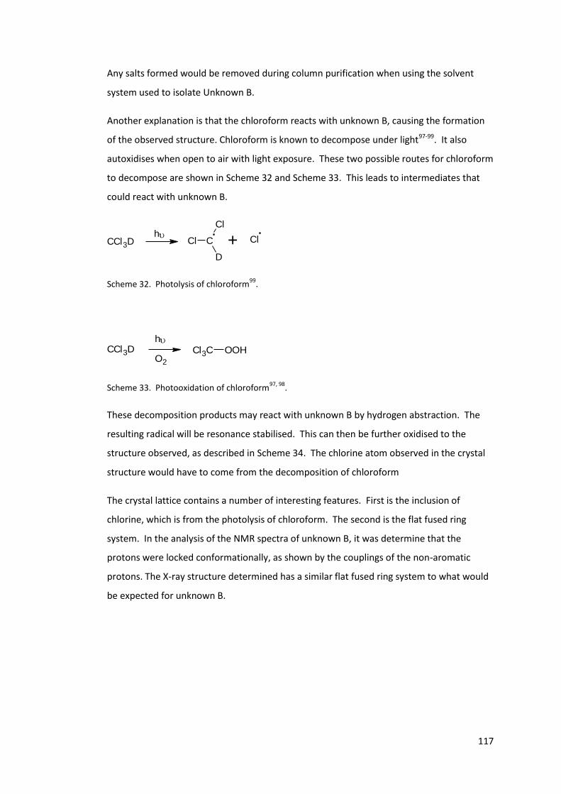
117
Any salts formed would be removed during column purification when using the solvent
system used to isolate Unknown B.
Another explanation is that the chloroform reacts with unknown B, causing the formation
of the observed structure. Chloroform is known to decompose under light97-99. It also
autoxidises when open to air with light exposure. These two possible routes for chloroform
to decompose are shown in Scheme 32 and Scheme 33. This leads to intermediates that
could react with unknown B.
CCl3Dh + ClCl C
D
Cl
Scheme 32. Photolysis of chloroform99
.
CCl3DO2
hCl3C OOH
Scheme 33. Photooxidation of chloroform97, 98
.
These decomposition products may react with unknown B by hydrogen abstraction. The
resulting radical will be resonance stabilised. This can then be further oxidised to the
structure observed, as described in Scheme 34. The chlorine atom observed in the crystal
structure would have to come from the decomposition of chloroform
The crystal lattice contains a number of interesting features. First is the inclusion of
chlorine, which is from the photolysis of chloroform. The second is the flat fused ring
system. In the analysis of the NMR spectra of unknown B, it was determine that the
protons were locked conformationally, as shown by the couplings of the non-aromatic
protons. The X-ray structure determined has a similar flat fused ring system to what would
be expected for unknown B.
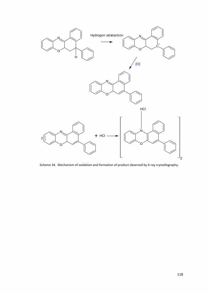
118
O
N
H
OC
N
O
N
[O]
Hydrogen abstraction
N
O
2
ClH
O
N
+ HCl2
Scheme 34. Mechanism of oxidation and formation of product observed by X-ray crystallography.
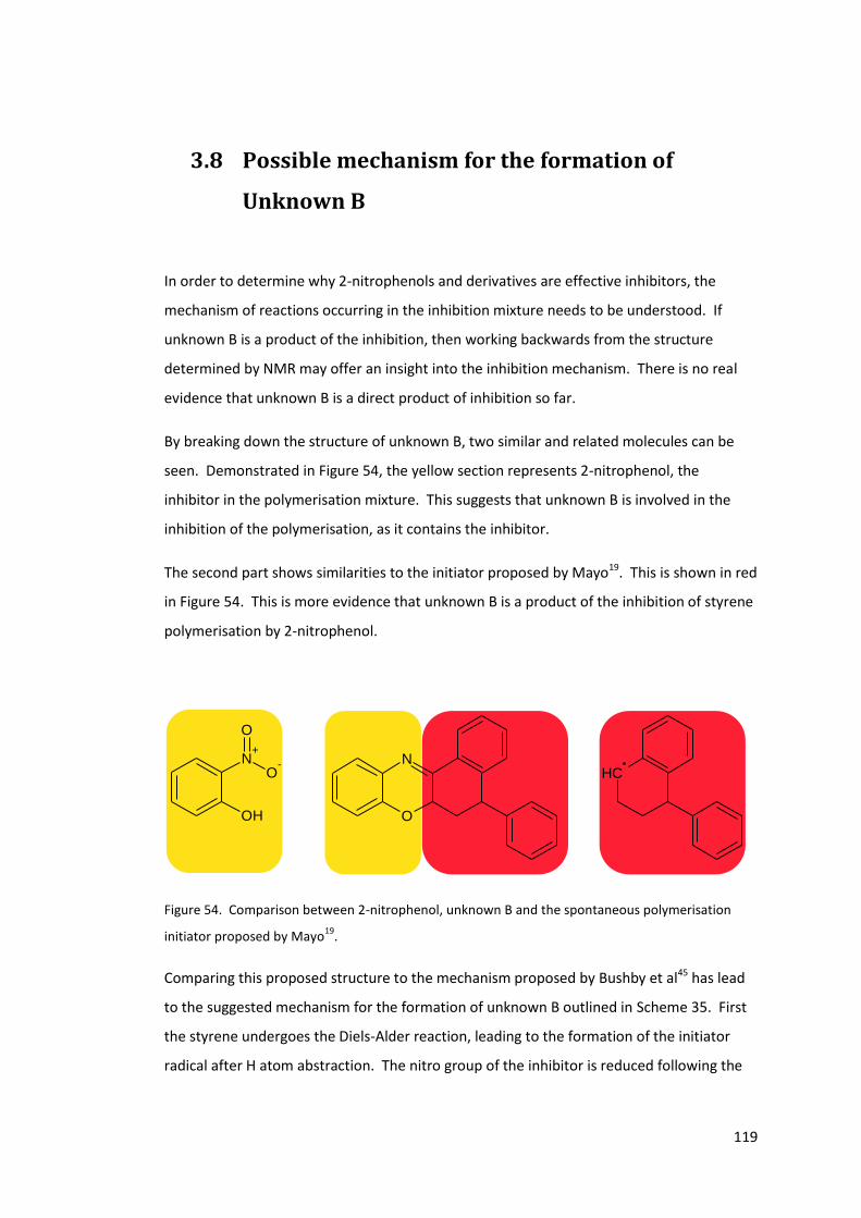
119
3.8 Possible mechanism for the formation of
Unknown B
In order to determine why 2-nitrophenols and derivatives are effective inhibitors, the
mechanism of reactions occurring in the inhibition mixture needs to be understood. If
unknown B is a product of the inhibition, then working backwards from the structure
determined by NMR may offer an insight into the inhibition mechanism. There is no real
evidence that unknown B is a direct product of inhibition so far.
By breaking down the structure of unknown B, two similar and related molecules can be
seen. Demonstrated in Figure 54, the yellow section represents 2-nitrophenol, the
inhibitor in the polymerisation mixture. This suggests that unknown B is involved in the
inhibition of the polymerisation, as it contains the inhibitor.
The second part shows similarities to the initiator proposed by Mayo19. This is shown in red
in Figure 54. This is more evidence that unknown B is a product of the inhibition of styrene
polymerisation by 2-nitrophenol.
CHN
O
N+
OH
O-
O
Figure 54. Comparison between 2-nitrophenol, unknown B and the spontaneous polymerisation
initiator proposed by Mayo19
.
Comparing this proposed structure to the mechanism proposed by Bushby et al45 has lead
to the suggested mechanism for the formation of unknown B outlined in Scheme 35. First
the styrene undergoes the Diels-Alder reaction, leading to the formation of the initiator
radical after H atom abstraction. The nitro group of the inhibitor is reduced following the
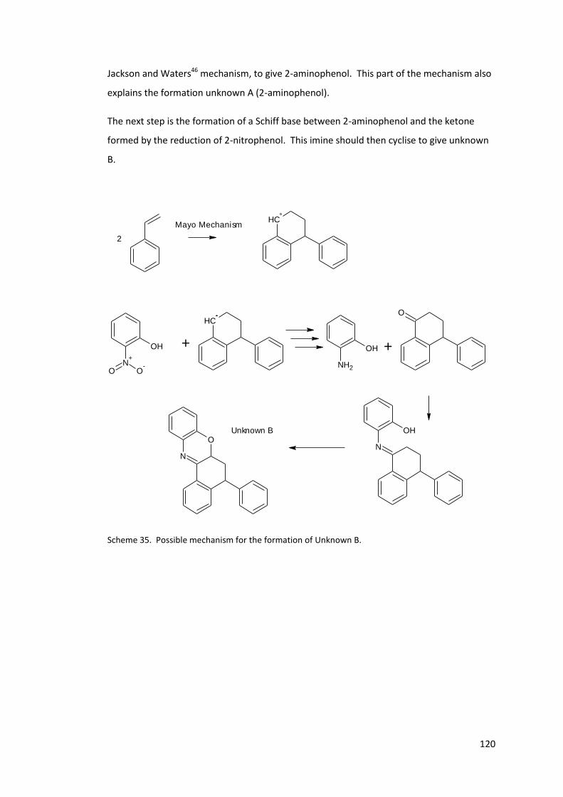
120
Jackson and Waters46 mechanism, to give 2-aminophenol. This part of the mechanism also
explains the formation unknown A (2-aminophenol).
The next step is the formation of a Schiff base between 2-aminophenol and the ketone
formed by the reduction of 2-nitrophenol. This imine should then cyclise to give unknown
B.
CH
OH
N+
O O-
CH
+ OH
NH2
O
+
N
OH
N
OUnknown B
2
Mayo Mechanism
Scheme 35. Possible mechanism for the formation of Unknown B.

121
3.9 Synthesis of the unknown B
The structure of unknown B product has been assigned with some confidence, but the
mechanism by which it is formed is still unknown. By synthesising it independently, the
way in which it is formed in the inhibition mechanism may also be explained. Scheme 36
shows the retro-synthetic analysis on the proposed structure for unknown B and the 2
possible starting materials needed. The synthesised compound will be referred to as
compound C to distinguish itself from the isolated unknown B. Interestingly, this appears
to follow the proposed mechanism in Scheme 35. Also one of the starting materials is 2-
aminophenol, the product isolated from the acid wash during the isolation of the product
(Unknown A). Once compound A is synthesised, comparing its physical properties and
spectra information should confirm the assignment from the NMR data obtained.
N
O
NH2
OH
O
Unknown A Compound DCompound C
Scheme 36. Retro-synthetic analysis of compound A.
2-Aminophenol is commercially available, however the ketone is not. Therefore it was
synthesised.
3.9.1 Ketone intermediate (Compound D)
The ketone was obtained following a procedure reported by Rendy et al100 and depicted in
Scheme 37. This will be referred to as compound D for clarity. The reaction follows a
similar route to a Haworth mechanism.101 The starting material is protonated by the triflic
acid, which is followed by a Friedel-Crafts reaction. The protonated carboxylic acid formed
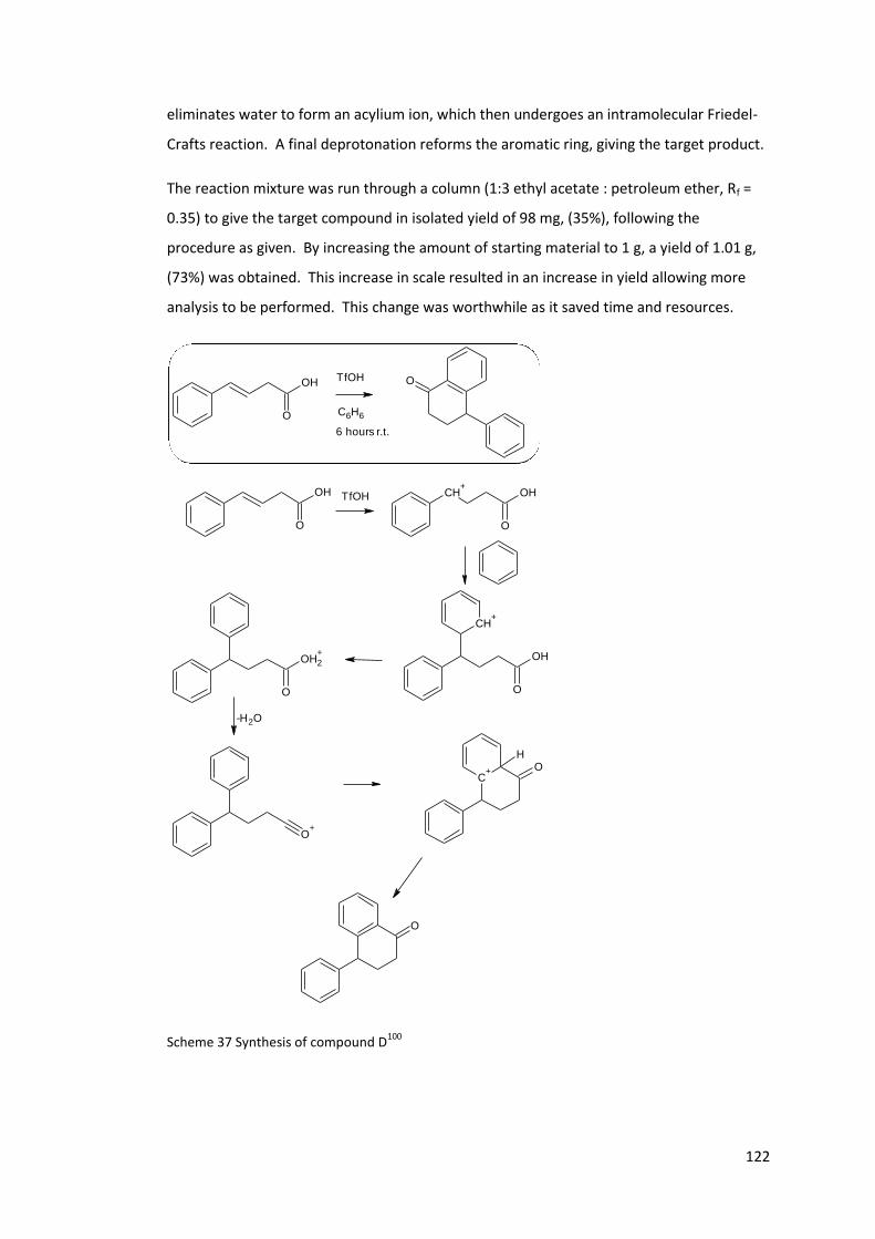
122
eliminates water to form an acylium ion, which then undergoes an intramolecular Friedel-
Crafts reaction. A final deprotonation reforms the aromatic ring, giving the target product.
The reaction mixture was run through a column (1:3 ethyl acetate : petroleum ether, Rf =
0.35) to give the target compound in isolated yield of 98 mg, (35%), following the
procedure as given. By increasing the amount of starting material to 1 g, a yield of 1.01 g,
(73%) was obtained. This increase in scale resulted in an increase in yield allowing more
analysis to be performed. This change was worthwhile as it saved time and resources.
OH
O
CH+
OH
O
OH
O
CH+
OH2
+
O
O+
C+ O
H
O
OH
O
TfOH
C6H6
6 hours r.t.
O
TfOH
-H2O
Scheme 37 Synthesis of compound D100

123
Unknown B was characterised by MS and NMR. The ESI MS gave a peak at m/z 222,
corresponding to [M + H]+. The proton NMR is given in Figure 55 and Figure 56. The NMR
spectra are labelled in the same way as previously, and these notations used in Table 6.
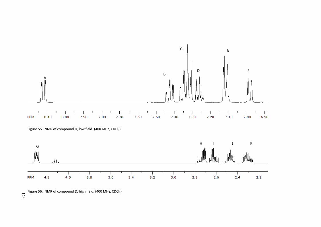
124
Figure 55. NMR of compound D, low field. (400 MHz, CDCl3)
Figure 56. NMR of compound D, high field. (400 MHz, CDCl3)
E
F D
C
B A
H I J K G
124
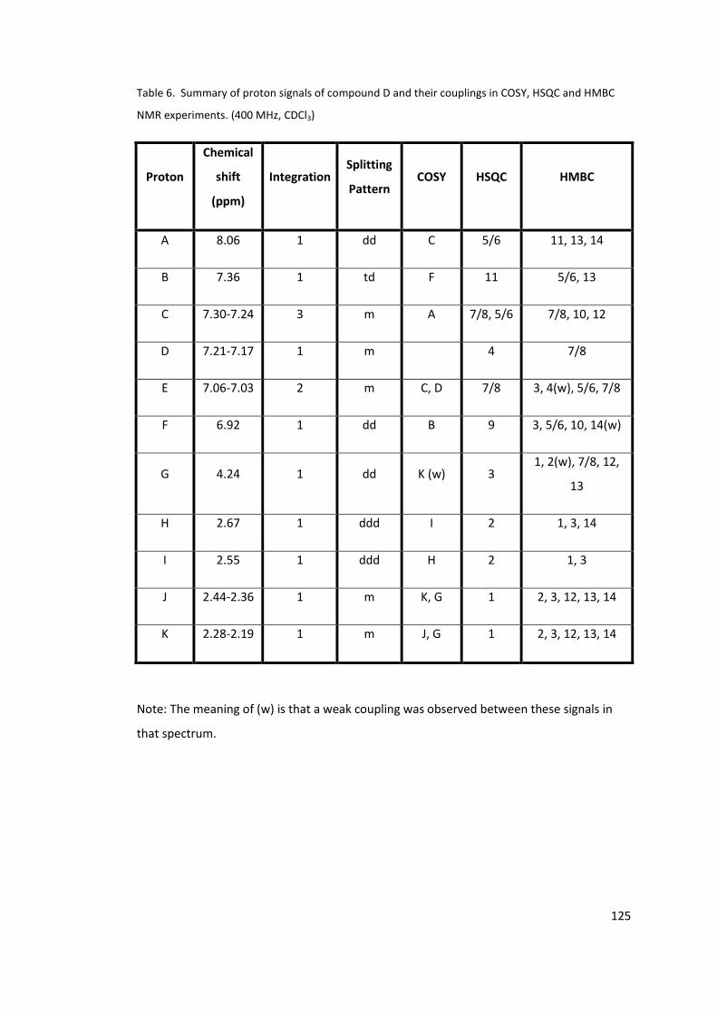
125
Table 6. Summary of proton signals of compound D and their couplings in COSY, HSQC and HMBC
NMR experiments. (400 MHz, CDCl3)
Proton
Chemical
shift
(ppm)
Integration Splitting
Pattern COSY HSQC HMBC
A 8.06 1 dd C 5/6 11, 13, 14
B 7.36 1 td F 11 5/6, 13
C 7.30-7.24 3 m A 7/8, 5/6 7/8, 10, 12
D 7.21-7.17 1 m 4 7/8
E 7.06-7.03 2 m C, D 7/8 3, 4(w), 5/6, 7/8
F 6.92 1 dd B 9 3, 5/6, 10, 14(w)
G 4.24 1 dd K (w) 3 1, 2(w), 7/8, 12,
13
H 2.67 1 ddd I 2 1, 3, 14
I 2.55 1 ddd H 2 1, 3
J 2.44-2.36 1 m K, G 1 2, 3, 12, 13, 14
K 2.28-2.19 1 m J, G 1 2, 3, 12, 13, 14
Note: The meaning of (w) is that a weak coupling was observed between these signals in
that spectrum.
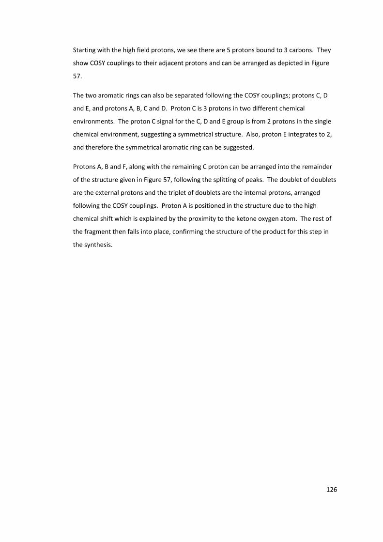
126
Starting with the high field protons, we see there are 5 protons bound to 3 carbons. They
show COSY couplings to their adjacent protons and can be arranged as depicted in Figure
57.
The two aromatic rings can also be separated following the COSY couplings; protons C, D
and E, and protons A, B, C and D. Proton C is 3 protons in two different chemical
environments. The proton C signal for the C, D and E group is from 2 protons in the single
chemical environment, suggesting a symmetrical structure. Also, proton E integrates to 2,
and therefore the symmetrical aromatic ring can be suggested.
Protons A, B and F, along with the remaining C proton can be arranged into the remainder
of the structure given in Figure 57, following the splitting of peaks. The doublet of doublets
are the external protons and the triplet of doublets are the internal protons, arranged
following the COSY couplings. Proton A is positioned in the structure due to the high
chemical shift which is explained by the proximity to the ketone oxygen atom. The rest of
the fragment then falls into place, confirming the structure of the product for this step in
the synthesis.
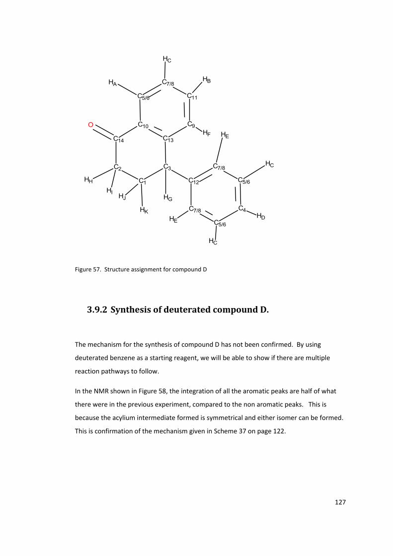
127
Figure 57. Structure assignment for compound D
3.9.2 Synthesis of deuterated compound D.
The mechanism for the synthesis of compound D has not been confirmed. By using
deuterated benzene as a starting reagent, we will be able to show if there are multiple
reaction pathways to follow.
In the NMR shown in Figure 58, the integration of all the aromatic peaks are half of what
there were in the previous experiment, compared to the non aromatic peaks. This is
because the acylium intermediate formed is symmetrical and either isomer can be formed.
This is confirmation of the mechanism given in Scheme 37 on page 122.

128
Figure 58. H1 NMR of ketone intermediate, synthesised using deuterated benzene. (400 MHz, CDCl3)
3.9.3 Synthesis of imine (Compound E)
The next step of the synthesis is to connect compound D and 2-aminophenol by forming an
imine (Compound E). The reaction is given in Scheme 38, following the procedure given by
Tauer et al102. The imine is moisture sensitive, as imines are, meaning the synthesis and
isolation must be done under inert atmosphere.
Even when leaving the reaction for long times (24 hours +), the reaction does not produce
pure imine. The NMR spectrum in Figure 60 shows that there is still starting material
present, and by comparing the integration between ketone and imine peaks, the yield is
1:1, imine : ketone. This also suggests that there is one equivalent of aminophenol
remaining in the mixture. This is confirmed by the MS spectra in Figure 59. The peak at
m/z 110 represents the remaining aminophenol, and the peaks at 222 and 245 m/z are the
[M+H]+ and [M+Na]+ peaks of the ketone.
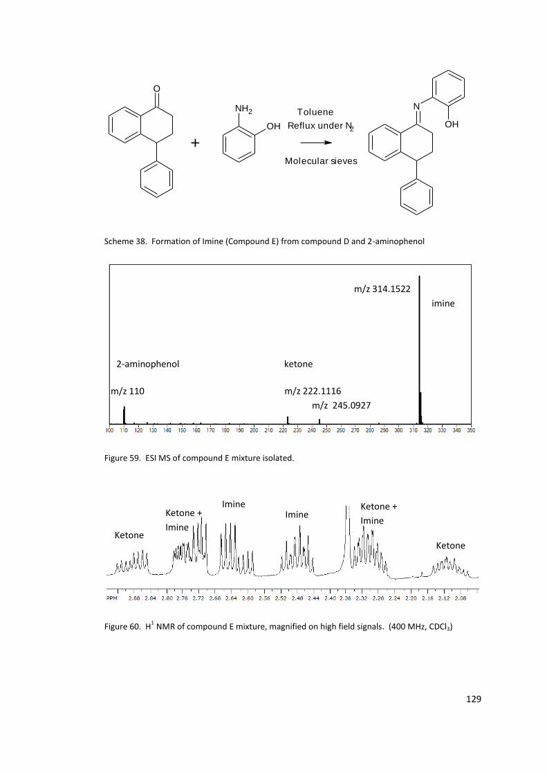
129
O
+
NH2
OH
N
OH
Toluene
Reflux under N2
Molecular sieves
Scheme 38. Formation of Imine (Compound E) from compound D and 2-aminophenol
Figure 59. ESI MS of compound E mixture isolated.
Figure 60. H1 NMR of compound E mixture, magnified on high field signals. (400 MHz, CDCl3)
imine
2-aminophenol
m/z 314.1522
ketone
m/z 222.1116
m/z 245.0927
m/z 110
Ketone +
Imine
Imine Ketone +
Imine
Imine
Ketone Ketone
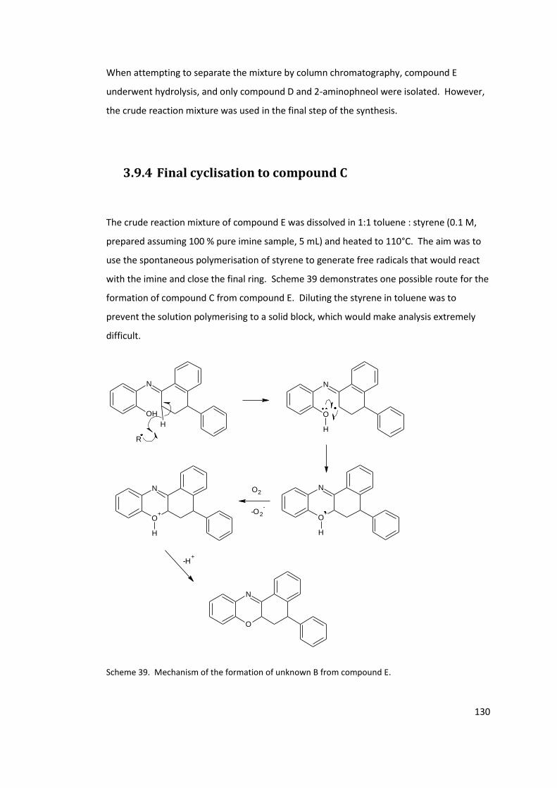
130
When attempting to separate the mixture by column chromatography, compound E
underwent hydrolysis, and only compound D and 2-aminophneol were isolated. However,
the crude reaction mixture was used in the final step of the synthesis.
3.9.4 Final cyclisation to compound C
The crude reaction mixture of compound E was dissolved in 1:1 toluene : styrene (0.1 M,
prepared assuming 100 % pure imine sample, 5 mL) and heated to 110°C. The aim was to
use the spontaneous polymerisation of styrene to generate free radicals that would react
with the imine and close the final ring. Scheme 39 demonstrates one possible route for the
formation of compound C from compound E. Diluting the styrene in toluene was to
prevent the solution polymerising to a solid block, which would make analysis extremely
difficult.
N
O+
H
N
OH
H
N
O
H
N
O+
H
N
O
O2
-O2
-
-H+
R
Scheme 39. Mechanism of the formation of unknown B from compound E.
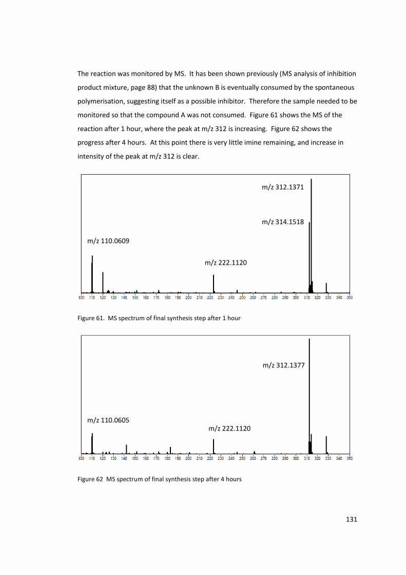
131
The reaction was monitored by MS. It has been shown previously (MS analysis of inhibition
product mixture, page 88) that the unknown B is eventually consumed by the spontaneous
polymerisation, suggesting itself as a possible inhibitor. Therefore the sample needed to be
monitored so that the compound A was not consumed. Figure 61 shows the MS of the
reaction after 1 hour, where the peak at m/z 312 is increasing. Figure 62 shows the
progress after 4 hours. At this point there is very little imine remaining, and increase in
intensity of the peak at m/z 312 is clear.
Figure 61. MS spectrum of final synthesis step after 1 hour
Figure 62 MS spectrum of final synthesis step after 4 hours
m/z 222.1120
m/z 312.1371
m/z 314.1518
m/z 110.0609
m/z 222.1120
m/z 312.1377
m/z 110.0605
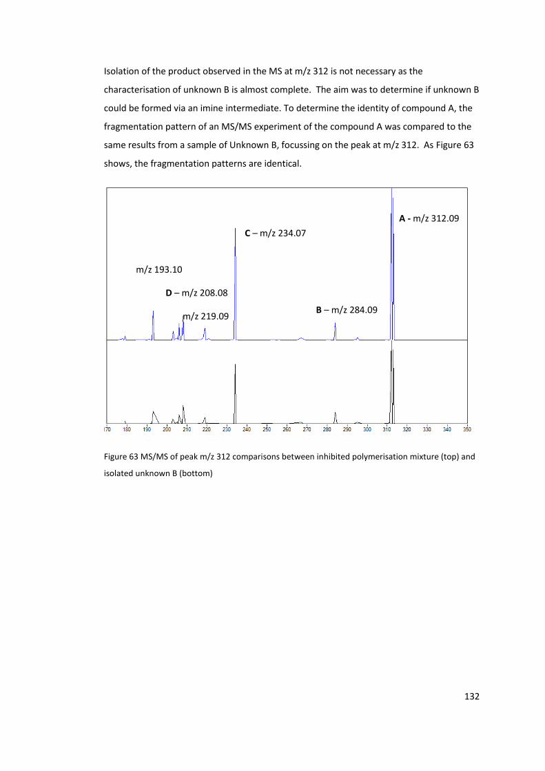
132
Isolation of the product observed in the MS at m/z 312 is not necessary as the
characterisation of unknown B is almost complete. The aim was to determine if unknown B
could be formed via an imine intermediate. To determine the identity of compound A, the
fragmentation pattern of an MS/MS experiment of the compound A was compared to the
same results from a sample of Unknown B, focussing on the peak at m/z 312. As Figure 63
shows, the fragmentation patterns are identical.
Figure 63 MS/MS of peak m/z 312 comparisons between inhibited polymerisation mixture (top) and
isolated unknown B (bottom)
m/z 193.10
D – m/z 208.08
m/z 219.09 B – m/z 284.09
C – m/z 234.07
A - m/z 312.09
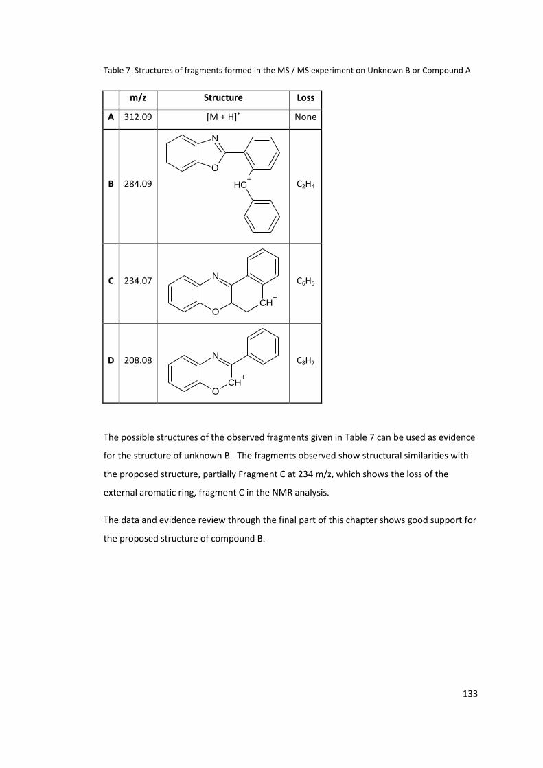
133
Table 7 Structures of fragments formed in the MS / MS experiment on Unknown B or Compound A
m/z Structure Loss
A 312.09 [M + H]+ None
B 284.09
N
O
CH+
C2H4
C 234.07 N
OCH
+
C6H5
D 208.08 N
OCH
+
C8H7
The possible structures of the observed fragments given in Table 7 can be used as evidence
for the structure of unknown B. The fragments observed show structural similarities with
the proposed structure, partially Fragment C at 234 m/z, which shows the loss of the
external aromatic ring, fragment C in the NMR analysis.
The data and evidence review through the final part of this chapter shows good support for
the proposed structure of compound B.
134
4. Intermediates in the inhibition of
spontaneous polymerisation of styrene by
nitrophenols
A number of intermediates and products have been identified in the spontaneous
polymerisation of styrene inhibited by 2-nitrophenol. The role of these intermediates and
products in the inhibition process is not clear. There are a number of different routes they
could take.
The intermediates observed may be the only inhibiting species in the mechanism, and need
to form first in order for the inhibitor to work. This would mean that factors, such as
stability of these intermediates, and the rate of their formation, would determine the
inhibition efficiency. If the intermediate is stable and formed quickly, then these
intermediate species would be readily available to react with the slow flux of initiators
formed spontaneously from styrene.
An alternative hypothesis is that these products are additional inhibitors formed from the
starting inhibitor, which would further inhibit the polymerisation. From the product
analysis we see that 2-aminophenol is formed from 2-nitrophenol during the inhibition of
polymerisation. It could be possible that these inhibit further. This is covered later in the
chapter.
Other possibilities are that these products no longer take part in inhibition or the products
and intermediates break down or further react via a non-inhibiting mechanism. This
effectively ends the inhibition mechanism.
An unlikely route is that these products initiate polymerisation, or form initiators in the
reaction mixture, effectively increasing the rate of polymerisation. This would be counter-
intuitive, as the aim of inhibitors is to stop the polymerisation, and any compound that
could give rise to an initiator would be avoided.
The aim of this chapter is to investigate the stability, reactivity and inhibition properties of
the intermediates proposed or observed in the last two chapters. The methods used will
involve the use of product analysis and dilatometry, similar to the previous study. The
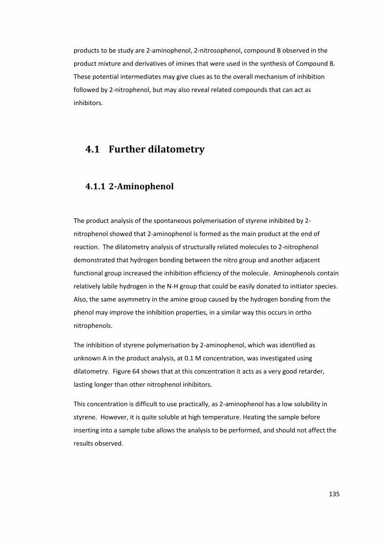
135
products to be study are 2-aminophenol, 2-nitrosophenol, compound B observed in the
product mixture and derivatives of imines that were used in the synthesis of Compound B.
These potential intermediates may give clues as to the overall mechanism of inhibition
followed by 2-nitrophenol, but may also reveal related compounds that can act as
inhibitors.
4.1 Further dilatometry
4.1.1 2-Aminophenol
The product analysis of the spontaneous polymerisation of styrene inhibited by 2-
nitrophenol showed that 2-aminophenol is formed as the main product at the end of
reaction. The dilatometry analysis of structurally related molecules to 2-nitrophenol
demonstrated that hydrogen bonding between the nitro group and another adjacent
functional group increased the inhibition efficiency of the molecule. Aminophenols contain
relatively labile hydrogen in the N-H group that could be easily donated to initiator species.
Also, the same asymmetry in the amine group caused by the hydrogen bonding from the
phenol may improve the inhibition properties, in a similar way this occurs in ortho
nitrophenols.
The inhibition of styrene polymerisation by 2-aminophenol, which was identified as
unknown A in the product analysis, at 0.1 M concentration, was investigated using
dilatometry. Figure 64 shows that at this concentration it acts as a very good retarder,
lasting longer than other nitrophenol inhibitors.
This concentration is difficult to use practically, as 2-aminophenol has a low solubility in
styrene. However, it is quite soluble at high temperature. Heating the sample before
inserting into a sample tube allows the analysis to be performed, and should not affect the
results observed.
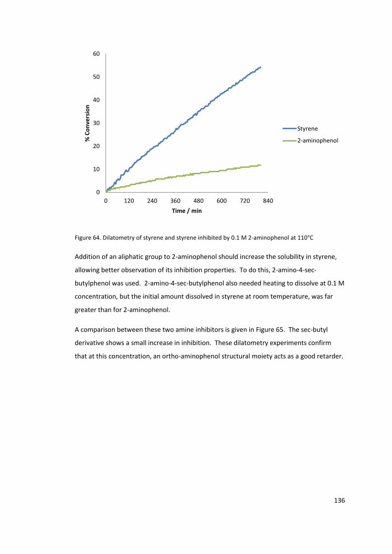
136
Figure 64. Dilatometry of styrene and styrene inhibited by 0.1 M 2-aminophenol at 110°C
Addition of an aliphatic group to 2-aminophenol should increase the solubility in styrene,
allowing better observation of its inhibition properties. To do this, 2-amino-4-sec-
butylphenol was used. 2-amino-4-sec-butylphenol also needed heating to dissolve at 0.1 M
concentration, but the initial amount dissolved in styrene at room temperature, was far
greater than for 2-aminophenol.
A comparison between these two amine inhibitors is given in Figure 65. The sec-butyl
derivative shows a small increase in inhibition. These dilatometry experiments confirm
that at this concentration, an ortho-aminophenol structural moiety acts as a good retarder.
0
10
20
30
40
50
60
0 120 240 360 480 600 720 840
% C
on
vers
ion
Time / min
Styrene
2-aminophenol
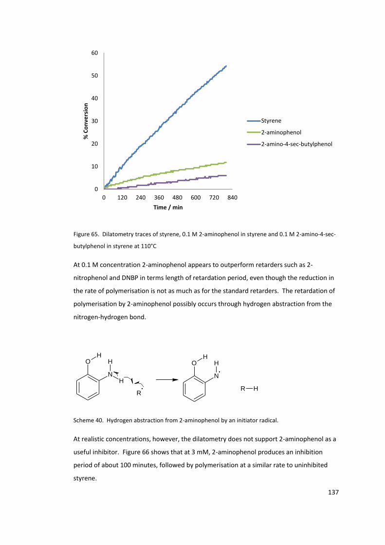
137
Figure 65. Dilatometry traces of styrene, 0.1 M 2-aminophenol in styrene and 0.1 M 2-amino-4-sec-
butylphenol in styrene at 110°C
At 0.1 M concentration 2-aminophenol appears to outperform retarders such as 2-
nitrophenol and DNBP in terms length of retardation period, even though the reduction in
the rate of polymerisation is not as much as for the standard retarders. The retardation of
polymerisation by 2-aminophenol possibly occurs through hydrogen abstraction from the
nitrogen-hydrogen bond.
O
NH
HH
R
O
N
HH
R H
Scheme 40. Hydrogen abstraction from 2-aminophenol by an initiator radical.
At realistic concentrations, however, the dilatometry does not support 2-aminophenol as a
useful inhibitor. Figure 66 shows that at 3 mM, 2-aminophenol produces an inhibition
period of about 100 minutes, followed by polymerisation at a similar rate to uninhibited
styrene.
0
10
20
30
40
50
60
0 120 240 360 480 600 720 840
% C
on
vers
ion
Time / min
Styrene
2-aminophenol
2-amino-4-sec-butylphenol
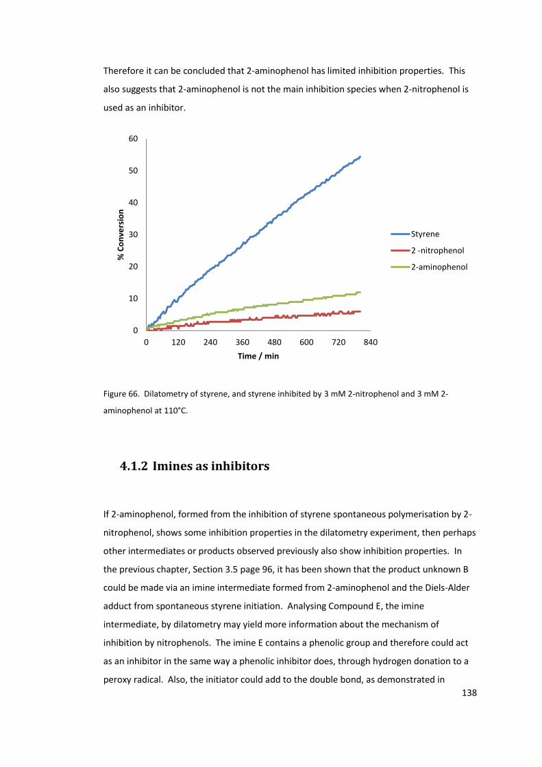
138
Therefore it can be concluded that 2-aminophenol has limited inhibition properties. This
also suggests that 2-aminophenol is not the main inhibition species when 2-nitrophenol is
used as an inhibitor.
Figure 66. Dilatometry of styrene, and styrene inhibited by 3 mM 2-nitrophenol and 3 mM 2-
aminophenol at 110°C.
4.1.2 Imines as inhibitors
If 2-aminophenol, formed from the inhibition of styrene spontaneous polymerisation by 2-
nitrophenol, shows some inhibition properties in the dilatometry experiment, then perhaps
other intermediates or products observed previously also show inhibition properties. In
the previous chapter, Section 3.5 page 96, it has been shown that the product unknown B
could be made via an imine intermediate formed from 2-aminophenol and the Diels-Alder
adduct from spontaneous styrene initiation. Analysing Compound E, the imine
intermediate, by dilatometry may yield more information about the mechanism of
inhibition by nitrophenols. The imine E contains a phenolic group and therefore could act
as an inhibitor in the same way a phenolic inhibitor does, through hydrogen donation to a
peroxy radical. Also, the initiator could add to the double bond, as demonstrated in
0
10
20
30
40
50
60
0 120 240 360 480 600 720 840
% C
on
vers
ion
Time / min
Styrene
2 -nitrophenol
2-aminophenol
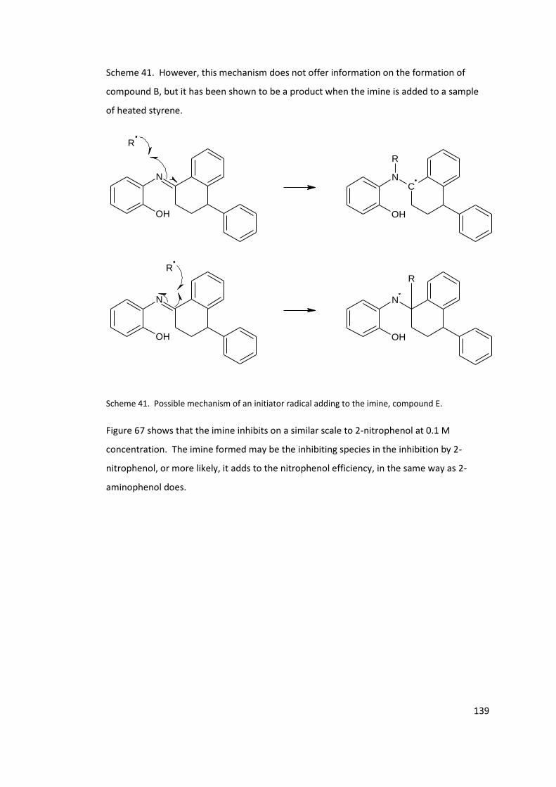
139
Scheme 41. However, this mechanism does not offer information on the formation of
compound B, but it has been shown to be a product when the imine is added to a sample
of heated styrene.
N
OH
R
NC
OH
R
N
OH
R
N
OH
R
Scheme 41. Possible mechanism of an initiator radical adding to the imine, compound E.
Figure 67 shows that the imine inhibits on a similar scale to 2-nitrophenol at 0.1 M
concentration. The imine formed may be the inhibiting species in the inhibition by 2-
nitrophenol, or more likely, it adds to the nitrophenol efficiency, in the same way as 2-
aminophenol does.
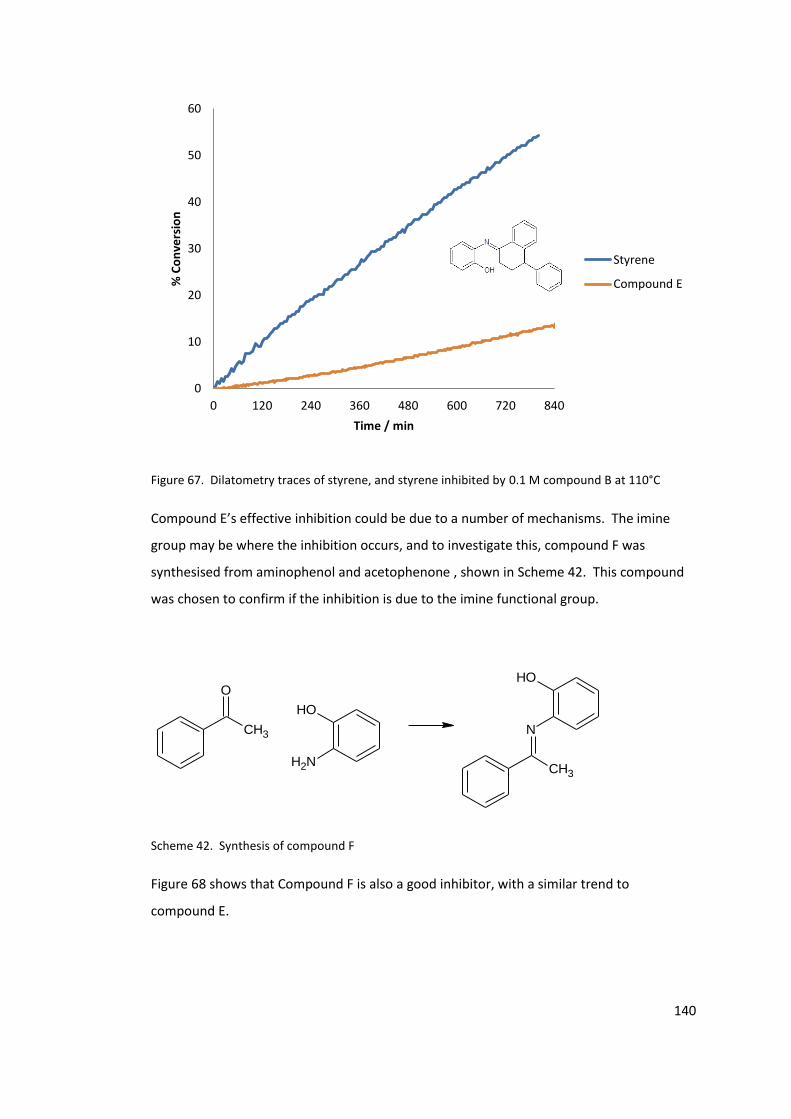
140
Figure 67. Dilatometry traces of styrene, and styrene inhibited by 0.1 M compound B at 110°C
Compound E’s effective inhibition could be due to a number of mechanisms. The imine
group may be where the inhibition occurs, and to investigate this, compound F was
synthesised from aminophenol and acetophenone , shown in Scheme 42. This compound
was chosen to confirm if the inhibition is due to the imine functional group.
CH3
O
NH2
OH
CH3
N
OH
Scheme 42. Synthesis of compound F
Figure 68 shows that Compound F is also a good inhibitor, with a similar trend to
compound E.
0
10
20
30
40
50
60
0 120 240 360 480 600 720 840
% C
on
vers
ion
Time / min
Styrene
Compound E
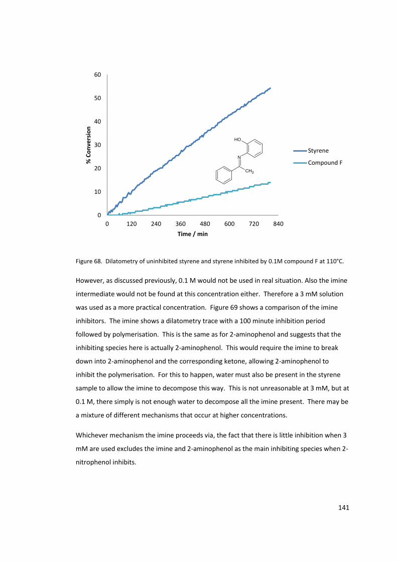
141
Figure 68. Dilatometry of uninhibited styrene and styrene inhibited by 0.1M compound F at 110°C.
However, as discussed previously, 0.1 M would not be used in real situation. Also the imine
intermediate would not be found at this concentration either. Therefore a 3 mM solution
was used as a more practical concentration. Figure 69 shows a comparison of the imine
inhibitors. The imine shows a dilatometry trace with a 100 minute inhibition period
followed by polymerisation. This is the same as for 2-aminophenol and suggests that the
inhibiting species here is actually 2-aminophenol. This would require the imine to break
down into 2-aminophenol and the corresponding ketone, allowing 2-aminophenol to
inhibit the polymerisation. For this to happen, water must also be present in the styrene
sample to allow the imine to decompose this way. This is not unreasonable at 3 mM, but at
0.1 M, there simply is not enough water to decompose all the imine present. There may be
a mixture of different mechanisms that occur at higher concentrations.
Whichever mechanism the imine proceeds via, the fact that there is little inhibition when 3
mM are used excludes the imine and 2-aminophenol as the main inhibiting species when 2-
nitrophenol inhibits.
0
10
20
30
40
50
60
0 120 240 360 480 600 720 840
% C
on
vers
ion
Time / min
Styrene
Compound F
CH3
N
OH
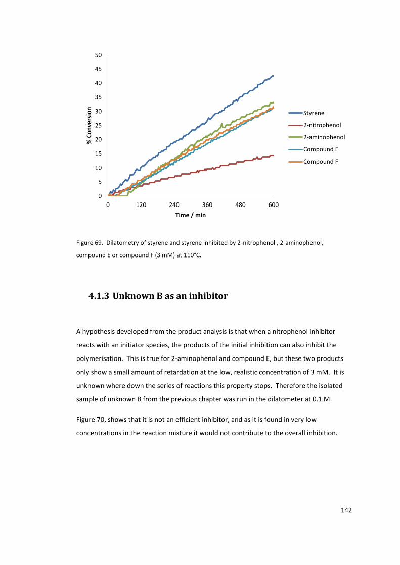
142
Figure 69. Dilatometry of styrene and styrene inhibited by 2-nitrophenol , 2-aminophenol,
compound E or compound F (3 mM) at 110°C.
4.1.3 Unknown B as an inhibitor
A hypothesis developed from the product analysis is that when a nitrophenol inhibitor
reacts with an initiator species, the products of the initial inhibition can also inhibit the
polymerisation. This is true for 2-aminophenol and compound E, but these two products
only show a small amount of retardation at the low, realistic concentration of 3 mM. It is
unknown where down the series of reactions this property stops. Therefore the isolated
sample of unknown B from the previous chapter was run in the dilatometer at 0.1 M.
Figure 70, shows that it is not an efficient inhibitor, and as it is found in very low
concentrations in the reaction mixture it would not contribute to the overall inhibition.
0
5
10
15
20
25
30
35
40
45
50
0 120 240 360 480 600
% C
on
vers
ion
Time / min
Styrene
2-nitrophenol
2-aminophenol
Compound E
Compound F
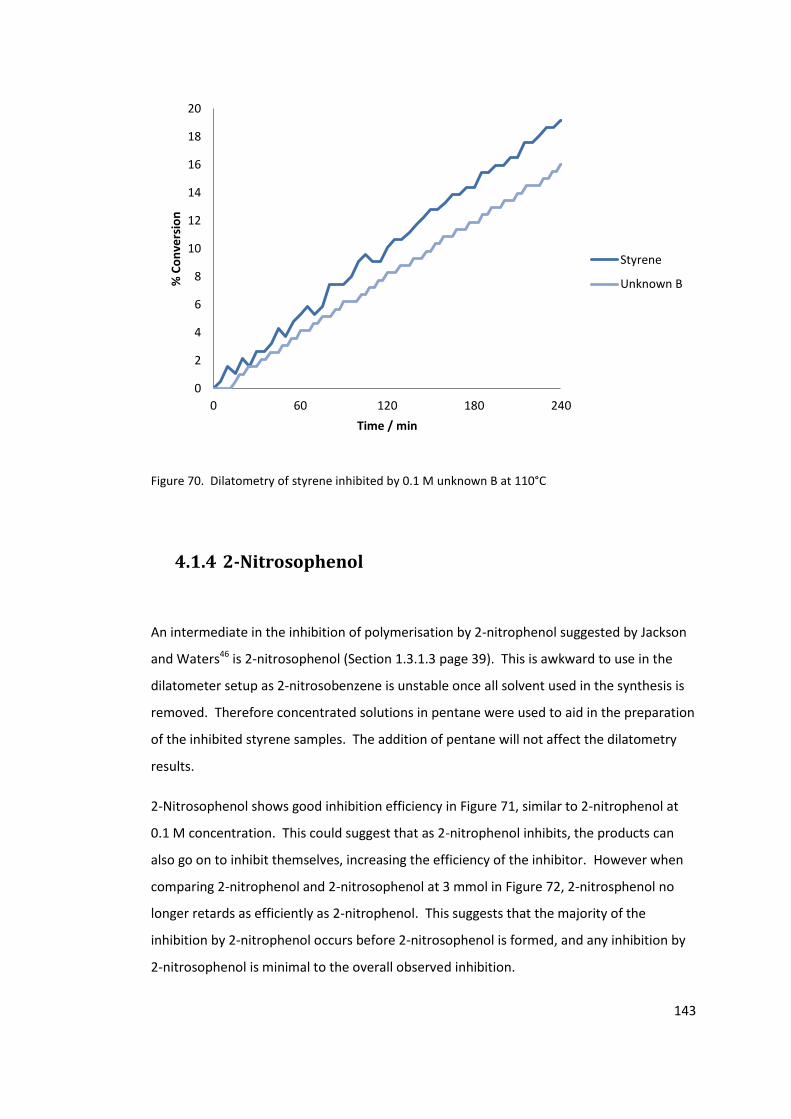
143
Figure 70. Dilatometry of styrene inhibited by 0.1 M unknown B at 110°C
4.1.4 2-Nitrosophenol
An intermediate in the inhibition of polymerisation by 2-nitrophenol suggested by Jackson
and Waters46 is 2-nitrosophenol (Section 1.3.1.3 page 39). This is awkward to use in the
dilatometer setup as 2-nitrosobenzene is unstable once all solvent used in the synthesis is
removed. Therefore concentrated solutions in pentane were used to aid in the preparation
of the inhibited styrene samples. The addition of pentane will not affect the dilatometry
results.
2-Nitrosophenol shows good inhibition efficiency in Figure 71, similar to 2-nitrophenol at
0.1 M concentration. This could suggest that as 2-nitrophenol inhibits, the products can
also go on to inhibit themselves, increasing the efficiency of the inhibitor. However when
comparing 2-nitrophenol and 2-nitrosophenol at 3 mmol in Figure 72, 2-nitrosphenol no
longer retards as efficiently as 2-nitrophenol. This suggests that the majority of the
inhibition by 2-nitrophenol occurs before 2-nitrosophenol is formed, and any inhibition by
2-nitrosophenol is minimal to the overall observed inhibition.
0
2
4
6
8
10
12
14
16
18
20
0 60 120 180 240
% C
on
vers
ion
Time / min
Styrene
Unknown B
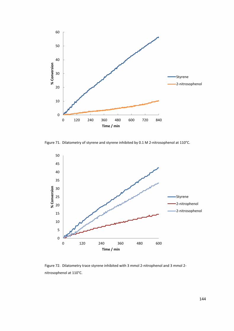
144
Figure 71. Dilatometry of styrene and styrene inhibited by 0.1 M 2-nitrosophenol at 110°C.
Figure 72. Dilatometry trace styrene inhibited with 3 mmol 2-nitrophenol and 3 mmol 2-
nitrosophenol at 110°C.
0
10
20
30
40
50
60
0 120 240 360 480 600 720 840
% C
on
vers
ion
Time / min
Styrene
2-nitrosophenol
0
5
10
15
20
25
30
35
40
45
50
0 120 240 360 480 600
% C
on
vers
ion
Time / min
Styrene
2-nitrophenol
2-nitrosophenol
145
4.2 Further product analysis
4.2.1 Nitroso intermediates
As discussed previously by Bartlett et al94 and Jackson and Waters46 (Section 1.3.1.3 page
39), nitroxides form in the nitrophenol inhibition of spontaneous styrene polymerisation,
via a nitroso intermediate (See Scheme 28 page 94). Formation of intermediate
nitrosophenol is also consistent with the reduction of 2-nitrophenol to 2-aminophenol
which was detected in the polymerisation mixture, (See section 3.5 page 96). The 2-
nitrosophenol intermediate may have the ability to react with the radical initiator species
and remove them from the propagation step. The reactivity of nitroso derivatives in the
styrene polymerisation may thus help us further understand the inhibition mechanism. This
section describes the investigation into these intermediates and tries to determine if they
are a major inhibiting species in a nitrophenol inhibition mechanism.
4.2.1.1 Nitrosobenzene
Nitrosobenzene was investigated first as a baseline for comparison to 2-nitrosophenol. As
demonstrated by dilatometry earlier, the position of the nitro and phenol groups affect the
inhibition properties of nitrophenol compounds. By looking first at nitrosobenzene, the
effect of ortho-hydroxy group on the inhibition properties of this compound can be
investigated.
Kang et al103 have studied the room temperature reaction between nitrosobenzene and
styrene and have identified the products formed. Their mechansim given in Scheme 43
shows the formation of isoxazolidines via a biradical intermediate, and the observed
products are labelled in the Scheme as compounds G and I. According to the authors, there
are two possible outcomes for the biradical. At room temperature compound H, the
nitrone, is observed and only after heating does this nitrone react with another molecule of
styrene to form compound I.

146
NO
NO
N
O
N
O
N+O
-
H H
N+O
-
H
+
RT
NO
226 m/z
198 m/z
Heat
+
RT
302 m/z
2
Compound G
Compound H
Compound I
Scheme 43. Literature proposed mechanism for reaction of nitrosobenzene and styrene. The m/z
values are the [M+H]+ ions observed
103.
An advantage of using nitrosobenzene as a potential inhibitor is that it is readily available,
unlike 2-nitrosophenol. When styrene is inhibited by nitrosobenzene, the reactions
described by Kang et al103 will take place very rapidly at high temperature and any
inhibition of polymerisation that is observed will be from the products of the reactions
described. Also, the authors have described a low temperature mechanism and a higher
temperature mechanism, with different products depending on the route.
Indeed, when making the solutions of nitrosobenzene in styrene for the dilatometer, an
observation was made. There was a steady colour change from red to dark brown over
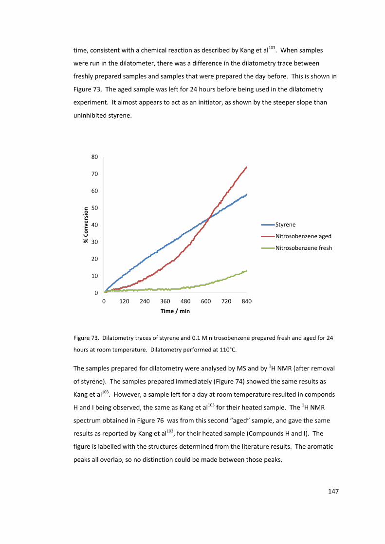
147
time, consistent with a chemical reaction as described by Kang et al103. When samples
were run in the dilatometer, there was a difference in the dilatometry trace between
freshly prepared samples and samples that were prepared the day before. This is shown in
Figure 73. The aged sample was left for 24 hours before being used in the dilatometry
experiment. It almost appears to act as an initiator, as shown by the steeper slope than
uninhibited styrene.
Figure 73. Dilatometry traces of styrene and 0.1 M nitrosobenzene prepared fresh and aged for 24
hours at room temperature. Dilatometry performed at 110°C.
The samples prepared for dilatometry were analysed by MS and by 1H NMR (after removal
of styrene). The samples prepared immediately (Figure 74) showed the same results as
Kang et al103. However, a sample left for a day at room temperature resulted in componds
H and I being observed, the same as Kang et al103 for their heated sample. The 1H NMR
spectrum obtained in Figure 76 was from this second “aged” sample, and gave the same
results as reported by Kang et al103, for their heated sample (Compounds H and I). The
figure is labelled with the structures determined from the literature results. The aromatic
peaks all overlap, so no distinction could be made between those peaks.
0
10
20
30
40
50
60
70
80
0 120 240 360 480 600 720 840
% C
on
vers
ion
Time / min
Styrene
Nitrosobenzene aged
Nitrosobenzene fresh
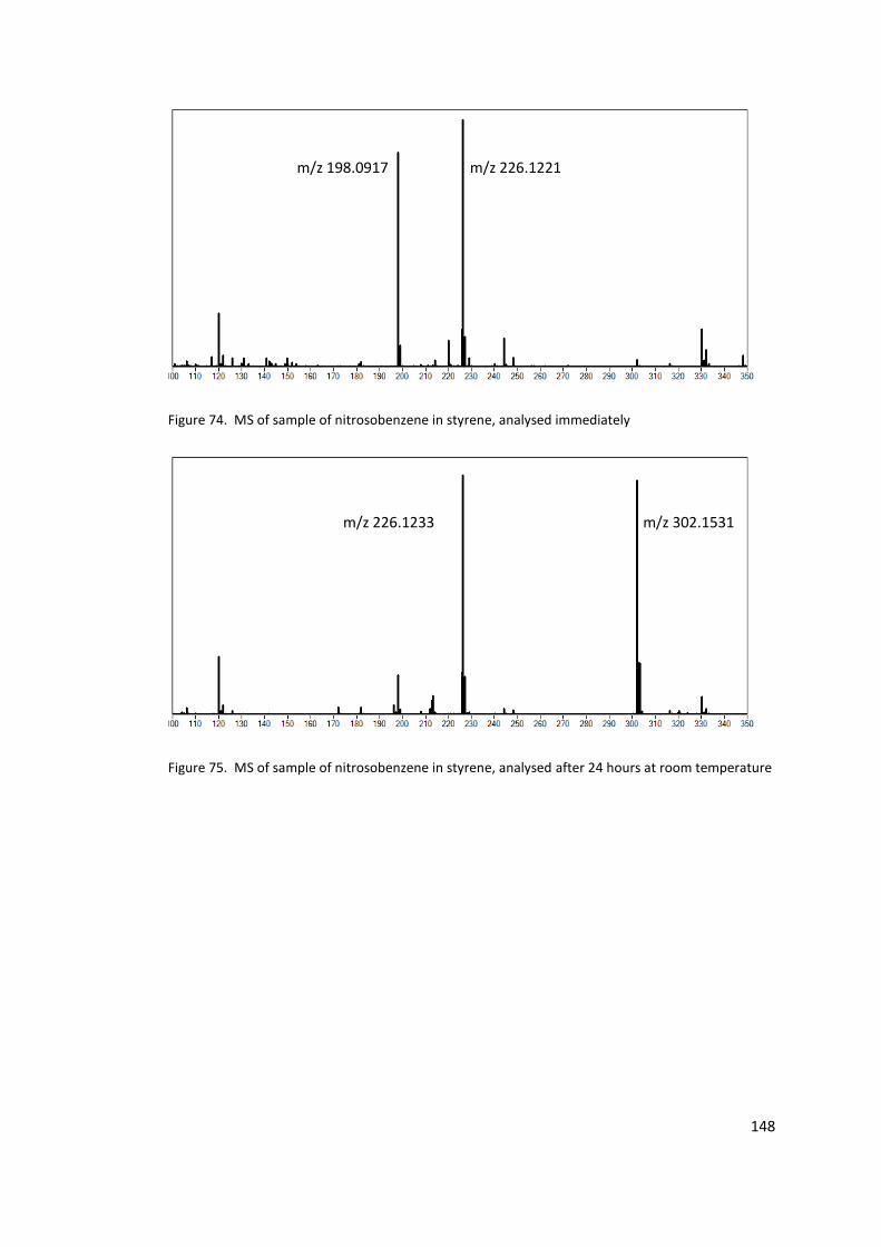
148
Figure 74. MS of sample of nitrosobenzene in styrene, analysed immediately
Figure 75. MS of sample of nitrosobenzene in styrene, analysed after 24 hours at room temperature
m/z 198.0917 m/z 226.1221
m/z 226.1233 m/z 302.1531
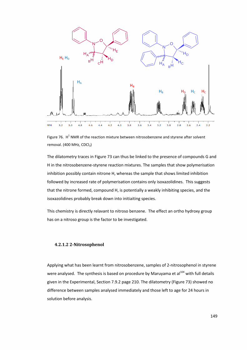
149
Figure 76. H1 NMR of the reaction mixture between nitrosobenzene and styrene after solvent
removal. (400 MHz, CDCl3)
The dilatometry traces in Figure 73 can thus be linked to the presence of compounds G and
H in the nitrosobenzene-styrene reaction mixtures. The samples that show polymerisation
inhibition possibly contain nitrone H, whereas the sample that shows limited inhibition
followed by increased rate of polymerisation contains only isoxazolidines. This suggests
that the nitrone formed, compound H, is potentially a weakly inhibiting species, and the
isoxazolidines probably break down into initiaiting species.
This chemistry is directly relavant to nitroso benzene. The effect an ortho hydroxy group
has on a nitroso group is the factor to be investigated.
4.2.1.2 2-Nitrosophenol
Applying what has been learnt from nitrosobenzene, samples of 2-nitrosophenol in styrene
were analysed. The synthesis is based on procedure by Maruyama et al104 with full details
given in the Experimental, Section 7.9.2 page 210. The dilatometry (Figure 73) showed no
difference between samples analysed immediately and those left to age for 24 hours in
solution before analysis.
HE HD
HA HB
HB HD HC HC
NO
HA
BHCH
HD
HE
NO
HA
HD
HCBH
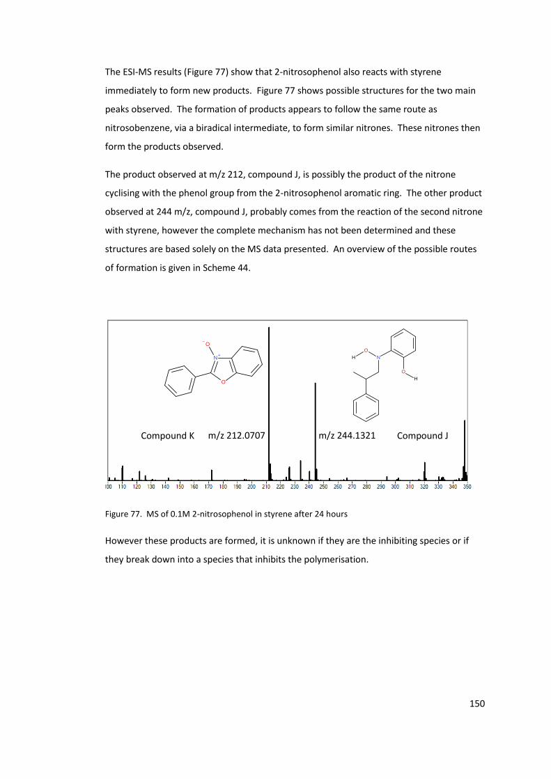
150
The ESI-MS results (Figure 77) show that 2-nitrosophenol also reacts with styrene
immediately to form new products. Figure 77 shows possible structures for the two main
peaks observed. The formation of products appears to follow the same route as
nitrosobenzene, via a biradical intermediate, to form similar nitrones. These nitrones then
form the products observed.
The product observed at m/z 212, compound J, is possibly the product of the nitrone
cyclising with the phenol group from the 2-nitrosophenol aromatic ring. The other product
observed at 244 m/z, compound J, probably comes from the reaction of the second nitrone
with styrene, however the complete mechanism has not been determined and these
structures are based solely on the MS data presented. An overview of the possible routes
of formation is given in Scheme 44.
Figure 77. MS of 0.1M 2-nitrosophenol in styrene after 24 hours
However these products are formed, it is unknown if they are the inhibiting species or if
they break down into a species that inhibits the polymerisation.
m/z 212.0707 m/z 244.1321 Compound K Compound J
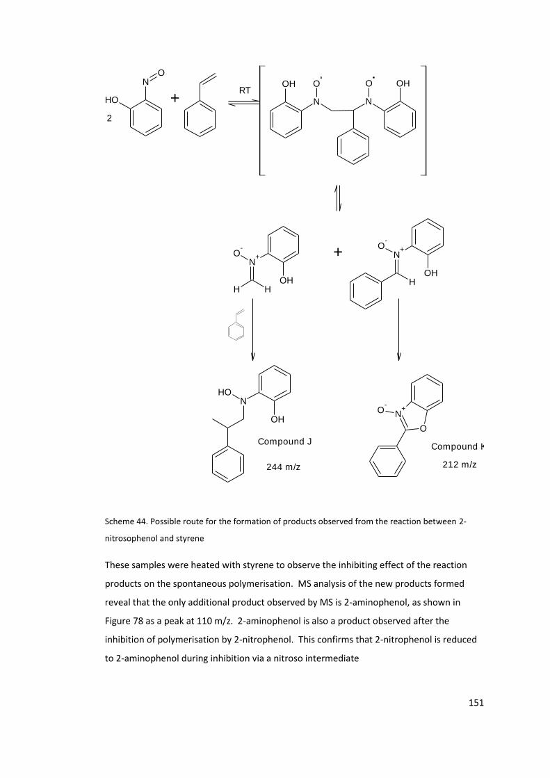
151
NO
OH N
O
N
OOH OH
N+O
-
HOH
+
RT+
2
O
N+O
-
N+O
-
H HOH
NOH
OH
Compound JCompound K
212 m/z244 m/z
Scheme 44. Possible route for the formation of products observed from the reaction between 2-
nitrosophenol and styrene
These samples were heated with styrene to observe the inhibiting effect of the reaction
products on the spontaneous polymerisation. MS analysis of the new products formed
reveal that the only additional product observed by MS is 2-aminophenol, as shown in
Figure 78 as a peak at 110 m/z. 2-aminophenol is also a product observed after the
inhibition of polymerisation by 2-nitrophenol. This confirms that 2-nitrophenol is reduced
to 2-aminophenol during inhibition via a nitroso intermediate
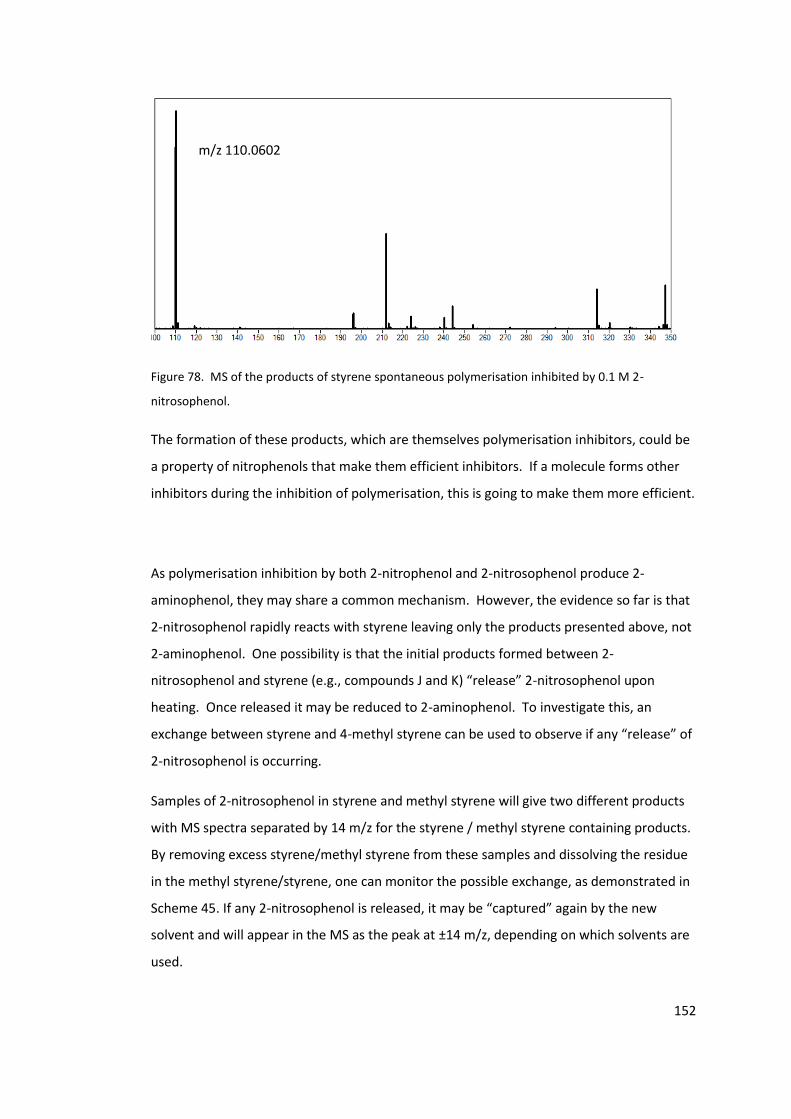
152
Figure 78. MS of the products of styrene spontaneous polymerisation inhibited by 0.1 M 2-
nitrosophenol.
The formation of these products, which are themselves polymerisation inhibitors, could be
a property of nitrophenols that make them efficient inhibitors. If a molecule forms other
inhibitors during the inhibition of polymerisation, this is going to make them more efficient.
As polymerisation inhibition by both 2-nitrophenol and 2-nitrosophenol produce 2-
aminophenol, they may share a common mechanism. However, the evidence so far is that
2-nitrosophenol rapidly reacts with styrene leaving only the products presented above, not
2-aminophenol. One possibility is that the initial products formed between 2-
nitrosophenol and styrene (e.g., compounds J and K) “release” 2-nitrosophenol upon
heating. Once released it may be reduced to 2-aminophenol. To investigate this, an
exchange between styrene and 4-methyl styrene can be used to observe if any “release” of
2-nitrosophenol is occurring.
Samples of 2-nitrosophenol in styrene and methyl styrene will give two different products
with MS spectra separated by 14 m/z for the styrene / methyl styrene containing products.
By removing excess styrene/methyl styrene from these samples and dissolving the residue
in the methyl styrene/styrene, one can monitor the possible exchange, as demonstrated in
Scheme 45. If any 2-nitrosophenol is released, it may be “captured” again by the new
solvent and will appear in the MS as the peak at ±14 m/z, depending on which solvents are
used.
m/z 110.0602
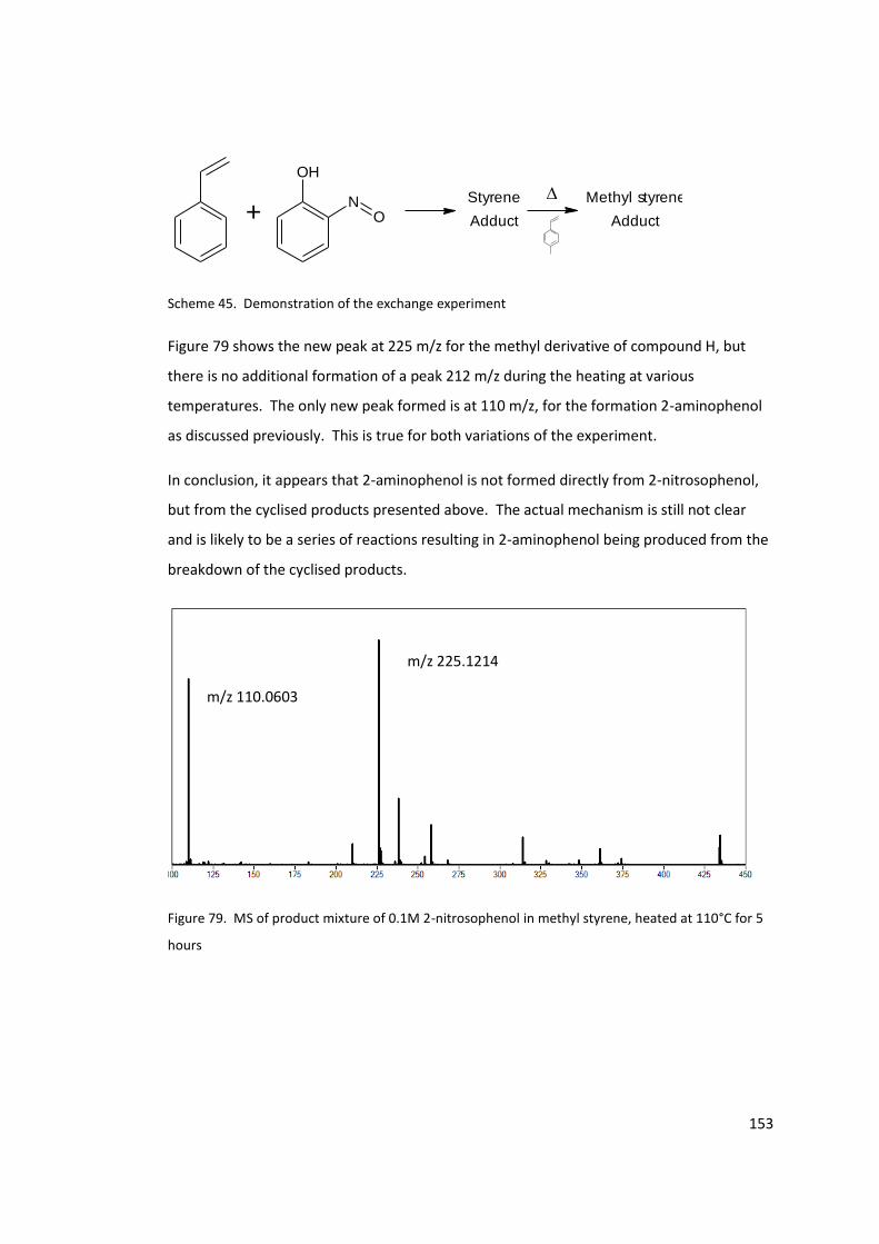
153
OH
NO+ Adduct
Styrene
Adduct
Methyl styrene
Scheme 45. Demonstration of the exchange experiment
Figure 79 shows the new peak at 225 m/z for the methyl derivative of compound H, but
there is no additional formation of a peak 212 m/z during the heating at various
temperatures. The only new peak formed is at 110 m/z, for the formation 2-aminophenol
as discussed previously. This is true for both variations of the experiment.
In conclusion, it appears that 2-aminophenol is not formed directly from 2-nitrosophenol,
but from the cyclised products presented above. The actual mechanism is still not clear
and is likely to be a series of reactions resulting in 2-aminophenol being produced from the
breakdown of the cyclised products.
Figure 79. MS of product mixture of 0.1M 2-nitrosophenol in methyl styrene, heated at 110°C for 5
hours
m/z 110.0603
m/z 225.1214
154
4.2.2 EPR of 2-nitrosophenol in styrene
In order to test if the reaction of 2-nitrosophenol with styrene involves free radical
intermediates, a solution of 0.1M 2-nitrosophenol in styrene was submitted for EPR
analysis. The black line in Figure 80 shows the spectrum obtained from the reaction
mixture prepared immediately before the sample was analysed. The concentration of
radical observed was ca. 0.1 mM at its maximum. This is 0.1% of the nitrosophenol used
and may not be an important intermediate of the reaction between styrene and 2-
nitrosophenol, but merely a by-product.
By simulating the spectrum, the structure of the radical can be obtained. The simulation is
given in Figure 80 as the red spectrum. There are two distinct hyperfine splitting, one from
the nitrogen of the nitroxide and another from two equivalent hydrogens. The simulation
gives the hyperfine values as aN as 10.17 G and aH as 3.46 G. These values are typical for
nitroxides with two α-hydrogens (Scheme 43), similar to results of Motyakin et al, 49 who
proposed a radical intermediate for the inhibition of styrene polymerisation inhibited by
2,4- dinitrophenol.
Interpretation of the spectra obtained show that there are at least two radical species in
the sample. There is the dominant species, which has been simulated, and a minor one,
too weak to properly identify. As shown previously, Section 3.4 page 94) the system is
complex, and again, complete identification of all species is not possible without
separation. This separation may not even be possible depending on the stability of the
radicals.
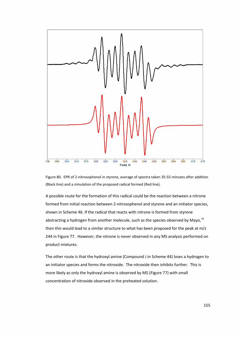
155
Figure 80. EPR of 2-nitrosophenol in styrene, average of spectra taken 35-55 minutes after addition
(Black line) and a simulation of the proposed radical formed (Red line).
A possible route for the formation of this radical could be the reaction between a nitrone
formed from initial reaction between 2-nitrosophenol and styrene and an initiator species,
shown in Scheme 46. If the radical that reacts with nitrone is formed from styrene
abstracting a hydrogen from another molecule, such as the species observed by Mayo,19
then this would lead to a similar structure to what has been proposed for the peak at m/z
244 in Figure 77. However, the nitrone is never observed in any MS analysis performed on
product mixtures.
The other route is that the hydroxyl amine (Compound J in Scheme 44) loses a hydrogen to
an initiator species and forms the nitroxide. The nitroxide then inhibits further. This is
more likely as only the hydroxyl amine is observed by MS (Figure 77) with small
concentration of nitroxide observed in the preheated solution.
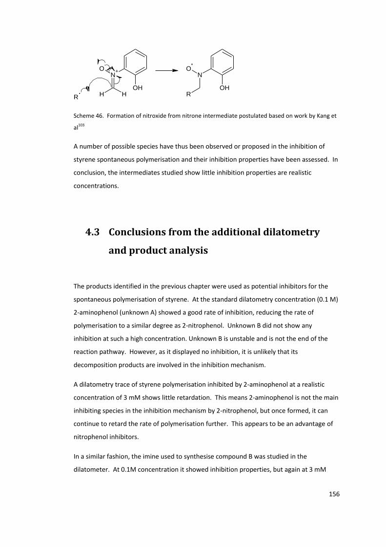
156
N+
OH
O-
H H
N
OH
O
RR
Scheme 46. Formation of nitroxide from nitrone intermediate postulated based on work by Kang et
al103
A number of possible species have thus been observed or proposed in the inhibition of
styrene spontaneous polymerisation and their inhibition properties have been assessed. In
conclusion, the intermediates studied show little inhibition properties are realistic
concentrations.
4.3 Conclusions from the additional dilatometry
and product analysis
The products identified in the previous chapter were used as potential inhibitors for the
spontaneous polymerisation of styrene. At the standard dilatometry concentration (0.1 M)
2-aminophenol (unknown A) showed a good rate of inhibition, reducing the rate of
polymerisation to a similar degree as 2-nitrophenol. Unknown B did not show any
inhibition at such a high concentration. Unknown B is unstable and is not the end of the
reaction pathway. However, as it displayed no inhibition, it is unlikely that its
decomposition products are involved in the inhibition mechanism.
A dilatometry trace of styrene polymerisation inhibited by 2-aminophenol at a realistic
concentration of 3 mM shows little retardation. This means 2-aminophenol is not the main
inhibiting species in the inhibition mechanism by 2-nitrophenol, but once formed, it can
continue to retard the rate of polymerisation further. This appears to be an advantage of
nitrophenol inhibitors.
In a similar fashion, the imine used to synthesise compound B was studied in the
dilatometer. At 0.1M concentration it showed inhibition properties, but again at 3 mM
157
there was no inhibition. This was also true for another imine synthesised, not related to
the inhibition mechanism, but for a comparison only.
2-Nitrosophenol was synthesised, but was shown to immediately react with styrene at
room temperature. In the inhibition mechanism by 2-nitrophenol, this would also occur,
rendering 2-nitrosophenol unable to inhibit. Upon heating these cyclised adducts release
2-aminophenol. This is a possible source of aminophenol for the formation of compound B.
4.4 The Mechanism of Inhibition
4.4.1 Is inhibition stoichiometric or catalytic?
If an inhibitor works via a cyclic, catalytic mechanism is going to be more efficient than a
stoichiometric mechanism. The inhibition by 2-nitrophenol is unknown as to whether it is
either of these scenarios. In order to determine this, the rate of radical production in
spontaneous self-polymerisation needs to be estimated and compare it to the rate at which
the inhibitor is lost. If the rates are similar, the mechanism is likely to be stoichiometric. If
the rate of inhibitor loss is much smaller than the rate of initiator production, the
mechanism is likely to be catalytic. The estimations presented below are just that,
estimates. Therefore an exact stoichiometric coefficient cannot be determined.
The mechanism of spontaneous polymerisation of styrene is covered in the Introduction,
Section 1.2.1 page 30. The initiator radicals form from the reaction between the styrene
dimer and another styrene monomer. Scheme 47 shows the simplified steps for the
formation of the initiator radicals. There are two steps, the formation of the dimer, D, from
the reaction of the monomer, M, and then the formation of the radicals, R.
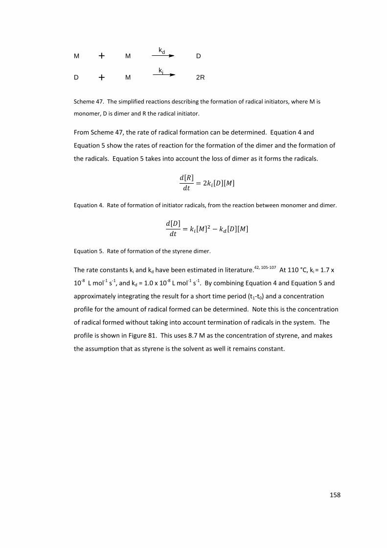
158
M M+
+ 2RMD
Dkd
ki
Scheme 47. The simplified reactions describing the formation of radical initiators, where M is
monomer, D is dimer and R the radical initiator.
From Scheme 47, the rate of radical formation can be determined. Equation 4 and
Equation 5 show the rates of reaction for the formation of the dimer and the formation of
the radicals. Equation 5 takes into account the loss of dimer as it forms the radicals.
𝑑[𝑅]
𝑑𝑡= 2𝑘𝑖[𝐷][𝑀]
Equation 4. Rate of formation of initiator radicals, from the reaction between monomer and dimer.
𝑑[𝐷]
𝑑𝑡= 𝑘𝑖[𝑀]
2 − 𝑘𝑑[𝐷][𝑀]
Equation 5. Rate of formation of the styrene dimer.
The rate constants ki and kd have been estimated in literature.42, 105-107 At 110 °C, ki = 1.7 x
10-8 L mol-1 s-1, and kd = 1.0 x 10⁻⁸ L mol-1 s-1. By combining Equation 4 and Equation 5 and
approximately integrating the result for a short time period (t1-t0) and a concentration
profile for the amount of radical formed can be determined. Note this is the concentration
of radical formed without taking into account termination of radicals in the system. The
profile is shown in Figure 81. This uses 8.7 M as the concentration of styrene, and makes
the assumption that as styrene is the solvent as well it remains constant.
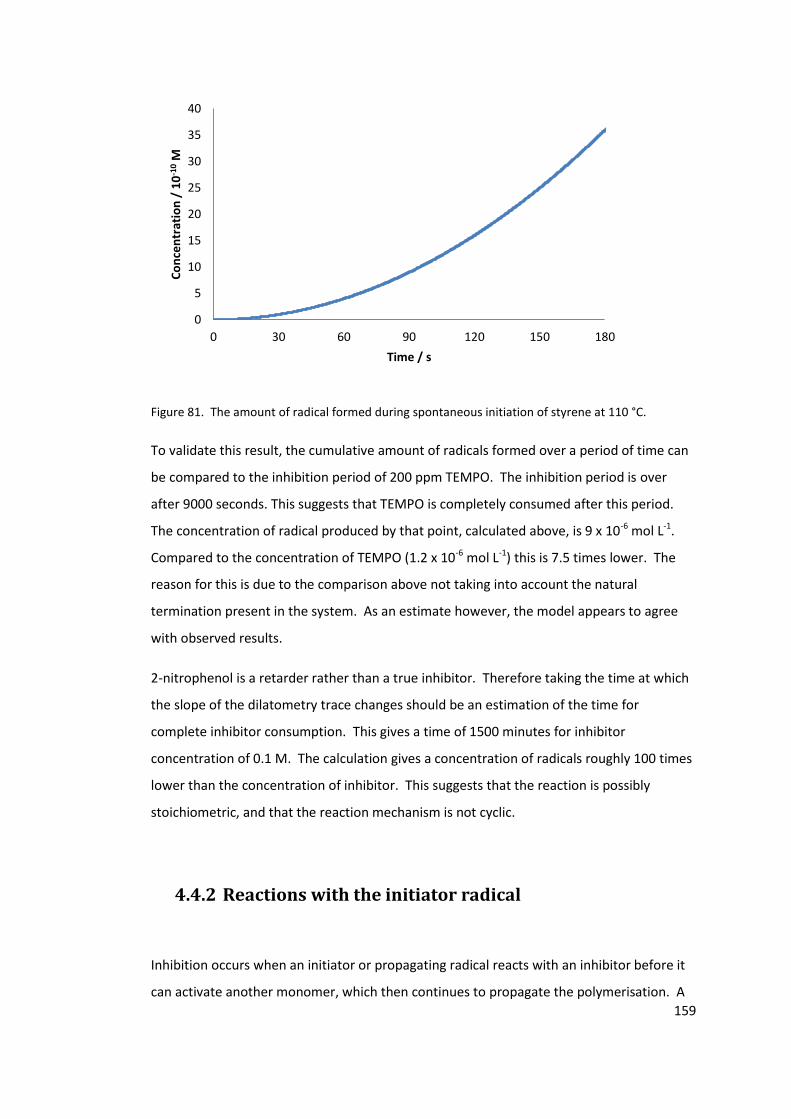
159
Figure 81. The amount of radical formed during spontaneous initiation of styrene at 110 °C.
To validate this result, the cumulative amount of radicals formed over a period of time can
be compared to the inhibition period of 200 ppm TEMPO. The inhibition period is over
after 9000 seconds. This suggests that TEMPO is completely consumed after this period.
The concentration of radical produced by that point, calculated above, is 9 x 10⁻⁶ mol L-1.
Compared to the concentration of TEMPO (1.2 x 10⁻⁶ mol L-1) this is 7.5 times lower. The
reason for this is due to the comparison above not taking into account the natural
termination present in the system. As an estimate however, the model appears to agree
with observed results.
2-nitrophenol is a retarder rather than a true inhibitor. Therefore taking the time at which
the slope of the dilatometry trace changes should be an estimation of the time for
complete inhibitor consumption. This gives a time of 1500 minutes for inhibitor
concentration of 0.1 M. The calculation gives a concentration of radicals roughly 100 times
lower than the concentration of inhibitor. This suggests that the reaction is possibly
stoichiometric, and that the reaction mechanism is not cyclic.
4.4.2 Reactions with the initiator radical
Inhibition occurs when an initiator or propagating radical reacts with an inhibitor before it
can activate another monomer, which then continues to propagate the polymerisation. A
0
5
10
15
20
25
30
35
40
0 30 60 90 120 150 180
Co
nce
ntr
atio
n /
10
-10
M
Time / s
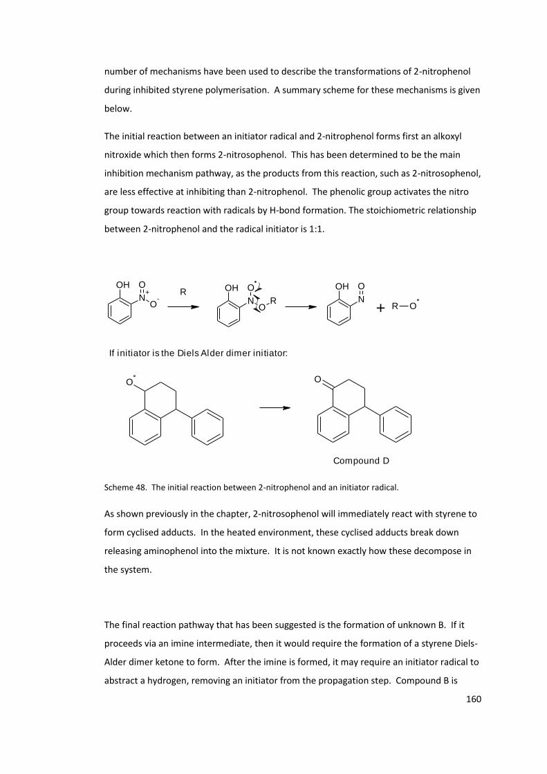
160
number of mechanisms have been used to describe the transformations of 2-nitrophenol
during inhibited styrene polymerisation. A summary scheme for these mechanisms is given
below.
The initial reaction between an initiator radical and 2-nitrophenol forms first an alkoxyl
nitroxide which then forms 2-nitrosophenol. This has been determined to be the main
inhibition mechanism pathway, as the products from this reaction, such as 2-nitrosophenol,
are less effective at inhibiting than 2-nitrophenol. The phenolic group activates the nitro
group towards reaction with radicals by H-bond formation. The stoichiometric relationship
between 2-nitrophenol and the radical initiator is 1:1.
OH
N+
O-
O OH
NO
O
R
OH
N
OR
+ R O
If initiator is the Diels Alder dimer initiator:
O O
Compound D
Scheme 48. The initial reaction between 2-nitrophenol and an initiator radical.
As shown previously in the chapter, 2-nitrosophenol will immediately react with styrene to
form cyclised adducts. In the heated environment, these cyclised adducts break down
releasing aminophenol into the mixture. It is not known exactly how these decompose in
the system.
The final reaction pathway that has been suggested is the formation of unknown B. If it
proceeds via an imine intermediate, then it would require the formation of a styrene Diels-
Alder dimer ketone to form. After the imine is formed, it may require an initiator radical to
abstract a hydrogen, removing an initiator from the propagation step. Compound B is
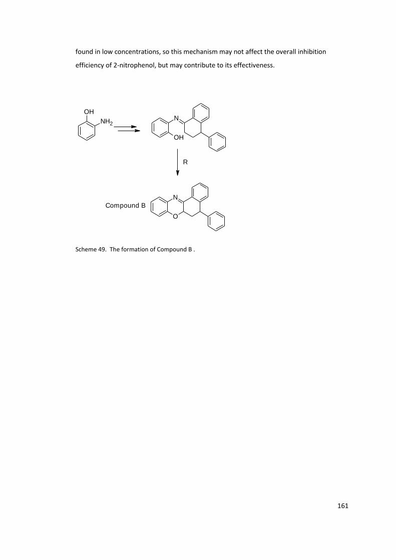
161
found in low concentrations, so this mechanism may not affect the overall inhibition
efficiency of 2-nitrophenol, but may contribute to its effectiveness.
OH
NH2N
OH
N
O
R
Compound B
Scheme 49. The formation of Compound B .
162
4.5 Conclusion
Investigating the reactivity of a number of intermediates in the 2-nitrophenol inhibited
spontaneous polymerisation of styrene, an inhibition pathway has been proposed. The
inhibition can be described as stoichiometric rather that a cyclic continuous mechanism,
although a stoichiometric coefficient cannot be accurately determined.
The start of the pathway begins with the hydrogen abstraction from nitrophenol, which is
facilitated by the intramolecular hydrogen bonding between the phenol and nitro groups.
Next is the formation of 2-nitrosophenol. This does not further inhibit, but immediately
reacts with styrene to form cycloadducts. These cycloadducts have been shown to
decompose at high temperature into aminophenol. This was identified in product mixtures
of styrene inhibited by 2-nitrophenol, and 2-nitrosophenol.
The final step of the reaction pathway is the formation of compound B, from 2-
aminophenol and a ketone derived from the Diels-Alder initiator molecule. It has been
demonstrated that the intermediates from this product formation, and the other
intermediate identified, show little to no inhibited properties. This strengthens the
conclusion that the initial step is where the inhibition occurs.
163
5. Chloranil Radical Anion
5.1 Introduction
Due to new EU legislation108, all chemicals produced above a certain amount need to be
valuated as to their toxic and environmental properties. This initiative is called the
Registration, Evaluation, Authorisation and Restriction of Chemicals, a.k.a. REACH. This will
eventually affect inhibitors such as DNBP. Nitro phenols are not without hazards, and will
need to be reassessed, with the possibility that they will no longer be allowed to be used.
Therefore the search for a new, green and non-toxic inhibitor has begun. This chapter aims
to continue the work of Yassin and Rizk61 into a charge transfer complex which acts as an
inhibitor.
5.1.1 A new inhibitor
As discussed in the introduction, quinones and hydroquinones have been used as
polymerisation inhibitors (Section 1.3.1.4 page 41). A paper by Yassin and Rizk61 proposed
that a charge transfer complex of 2,3,5,6-tetrachlorocyclohexa-2,5-diene-1,4-dione
(Chloranil) to N, N-dimethyl aniline (DMA), acts as a polymerisation inhibitor. The
degradation of the charge transfer complex leads to the chloranil radical anion, also known
as a semiquinone, which is believed to be the inhibiting species.
Scheme 50 shows the structure of the charge transfer complex which Yassin and Rizk
investigated. The first equilibrium shows the formation of the charge transfer complex of
DMA and chloranil. The second equilibrium may possibly not be established under reaction
conditions, as further reactions of radicals formed will compete with their recombination.
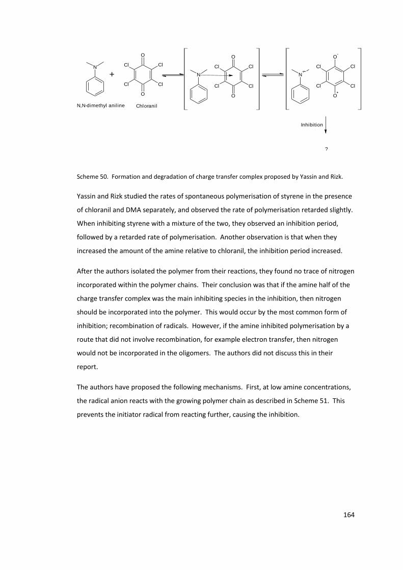
164
N
O
O
Cl
Cl
Cl
Cl
+ N
O
O
Cl
Cl
Cl
Cl
N+
O-
O
Cl
Cl
Cl
Cl
Inhibition
?
N,N-dimethyl anil ine Chloranil
Scheme 50. Formation and degradation of charge transfer complex proposed by Yassin and Rizk.
Yassin and Rizk studied the rates of spontaneous polymerisation of styrene in the presence
of chloranil and DMA separately, and observed the rate of polymerisation retarded slightly.
When inhibiting styrene with a mixture of the two, they observed an inhibition period,
followed by a retarded rate of polymerisation. Another observation is that when they
increased the amount of the amine relative to chloranil, the inhibition period increased.
After the authors isolated the polymer from their reactions, they found no trace of nitrogen
incorporated within the polymer chains. Their conclusion was that if the amine half of the
charge transfer complex was the main inhibiting species in the inhibition, then nitrogen
should be incorporated into the polymer. This would occur by the most common form of
inhibition; recombination of radicals. However, if the amine inhibited polymerisation by a
route that did not involve recombination, for example electron transfer, then nitrogen
would not be incorporated in the oligomers. The authors did not discuss this in their
report.
The authors have proposed the following mechanisms. First, at low amine concentrations,
the radical anion reacts with the growing polymer chain as described in Scheme 51. This
prevents the initiator radical from reacting further, causing the inhibition.
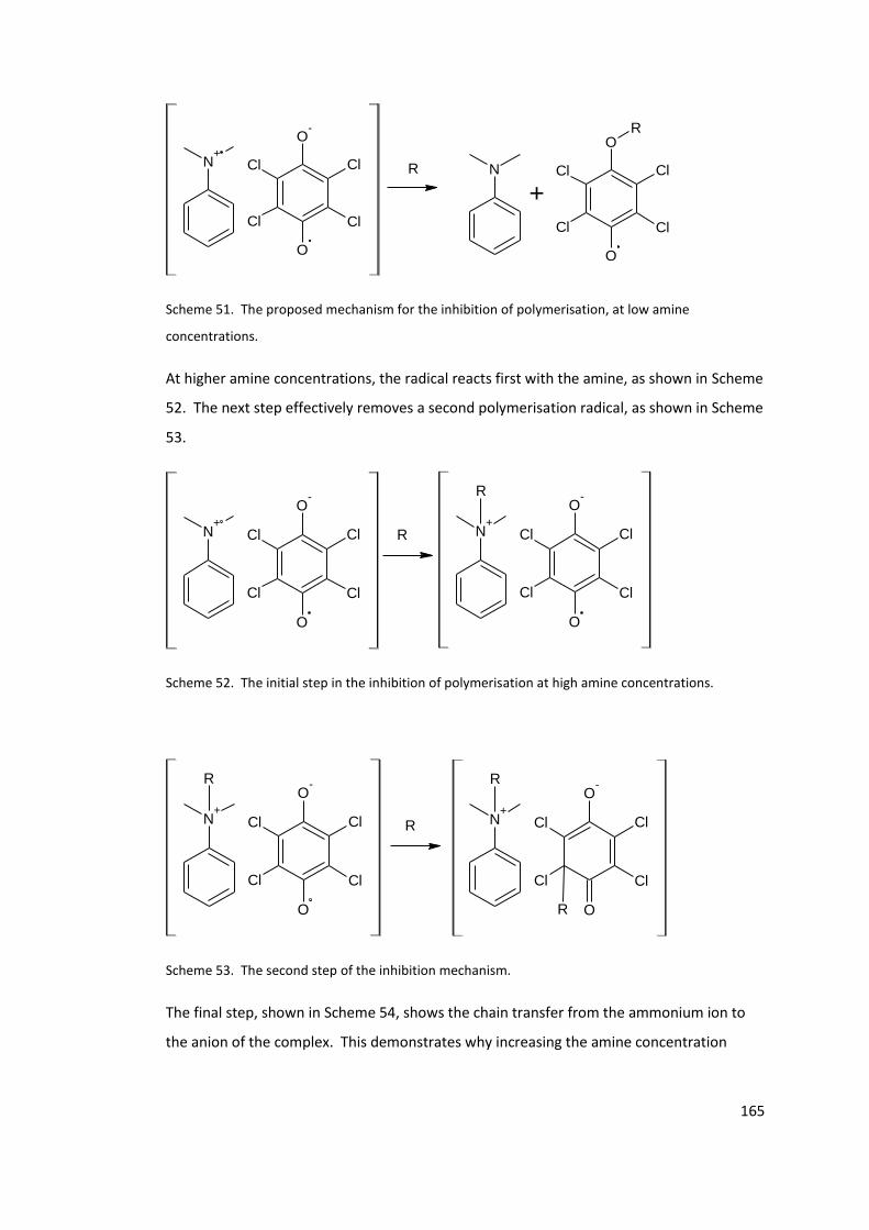
165
N+
O-
O
Cl
ClCl
Cl
R N
O
O
Cl
ClCl
Cl
R
+
Scheme 51. The proposed mechanism for the inhibition of polymerisation, at low amine
concentrations.
At higher amine concentrations, the radical reacts first with the amine, as shown in Scheme
52. The next step effectively removes a second polymerisation radical, as shown in Scheme
53.
N+
O-
O
Cl
ClCl
Cl
N+
RO
-
O
Cl
ClCl
Cl
R
Scheme 52. The initial step in the inhibition of polymerisation at high amine concentrations.
N+
RO
-
O
Cl
ClCl
Cl
R N+
RO
-
O
Cl
ClCl
Cl
R
Scheme 53. The second step of the inhibition mechanism.
The final step, shown in Scheme 54, shows the chain transfer from the ammonium ion to
the anion of the complex. This demonstrates why increasing the amine concentration
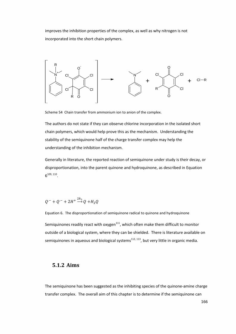
166
improves the inhibition properties of the complex, as well as why nitrogen is not
incorporated into the short chain polymers.
N+
RO
-
O
Cl
ClCl
Cl
R
N
O
O
Cl
ClCl
R
Cl R+ +
Scheme 54 Chain transfer from ammonium ion to anion of the complex.
The authors do not state if they can observe chlorine incorporation in the isolated short
chain polymers, which would help prove this as the mechanism. Understanding the
stability of the semiquinone half of the charge transfer complex may help the
understanding of the inhibition mechanism.
Generally in literature, the reported reaction of semiquinone under study is their decay, or
disproportionation, into the parent quinone and hydroquinone, as described in Equation
6109, 110.
𝑄.− + 𝑄.− + 2𝐻+2𝑘1→ 𝑄 +𝐻2𝑄
Equation 6. The disproportionation of semiquinone radical to quinone and hydroquinone
Semiquinones readily react with oxygen111, which often make them difficult to monitor
outside of a biological system, where they can be shielded. There is literature available on
semiquinones in aqueous and biological systems112, 113, but very little in organic media.
5.1.2 Aims
The semiquinone has been suggested as the inhibiting species of the quinone-amine charge
transfer complex. The overall aim of this chapter is to determine if the semiquinone can
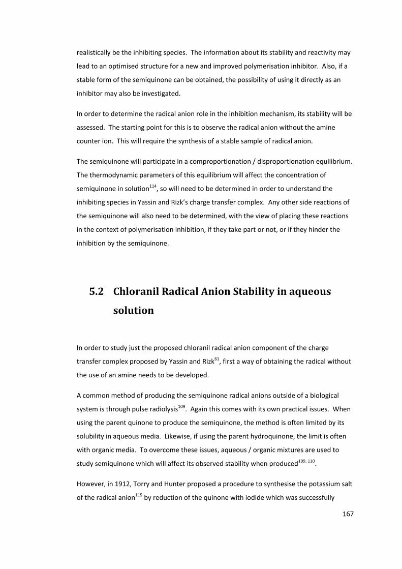
167
realistically be the inhibiting species. The information about its stability and reactivity may
lead to an optimised structure for a new and improved polymerisation inhibitor. Also, if a
stable form of the semiquinone can be obtained, the possibility of using it directly as an
inhibitor may also be investigated.
In order to determine the radical anion role in the inhibition mechanism, its stability will be
assessed. The starting point for this is to observe the radical anion without the amine
counter ion. This will require the synthesis of a stable sample of radical anion.
The semiquinone will participate in a comproportionation / disproportionation equilibrium.
The thermodynamic parameters of this equilibrium will affect the concentration of
semiquinone in solution114, so will need to be determined in order to understand the
inhibiting species in Yassin and Rizk’s charge transfer complex. Any other side reactions of
the semiquinone will also need to be determined, with the view of placing these reactions
in the context of polymerisation inhibition, if they take part or not, or if they hinder the
inhibition by the semiquinone.
5.2 Chloranil Radical Anion Stability in aqueous
solution
In order to study just the proposed chloranil radical anion component of the charge
transfer complex proposed by Yassin and Rizk61, first a way of obtaining the radical without
the use of an amine needs to be developed.
A common method of producing the semiquinone radical anions outside of a biological
system is through pulse radiolysis109. Again this comes with its own practical issues. When
using the parent quinone to produce the semiquinone, the method is often limited by its
solubility in aqueous media. Likewise, if using the parent hydroquinone, the limit is often
with organic media. To overcome these issues, aqueous / organic mixtures are used to
study semiquinone which will affect its observed stability when produced109, 110.
However, in 1912, Torry and Hunter proposed a procedure to synthesise the potassium salt
of the radical anion115 by reduction of the quinone with iodide which was successfully
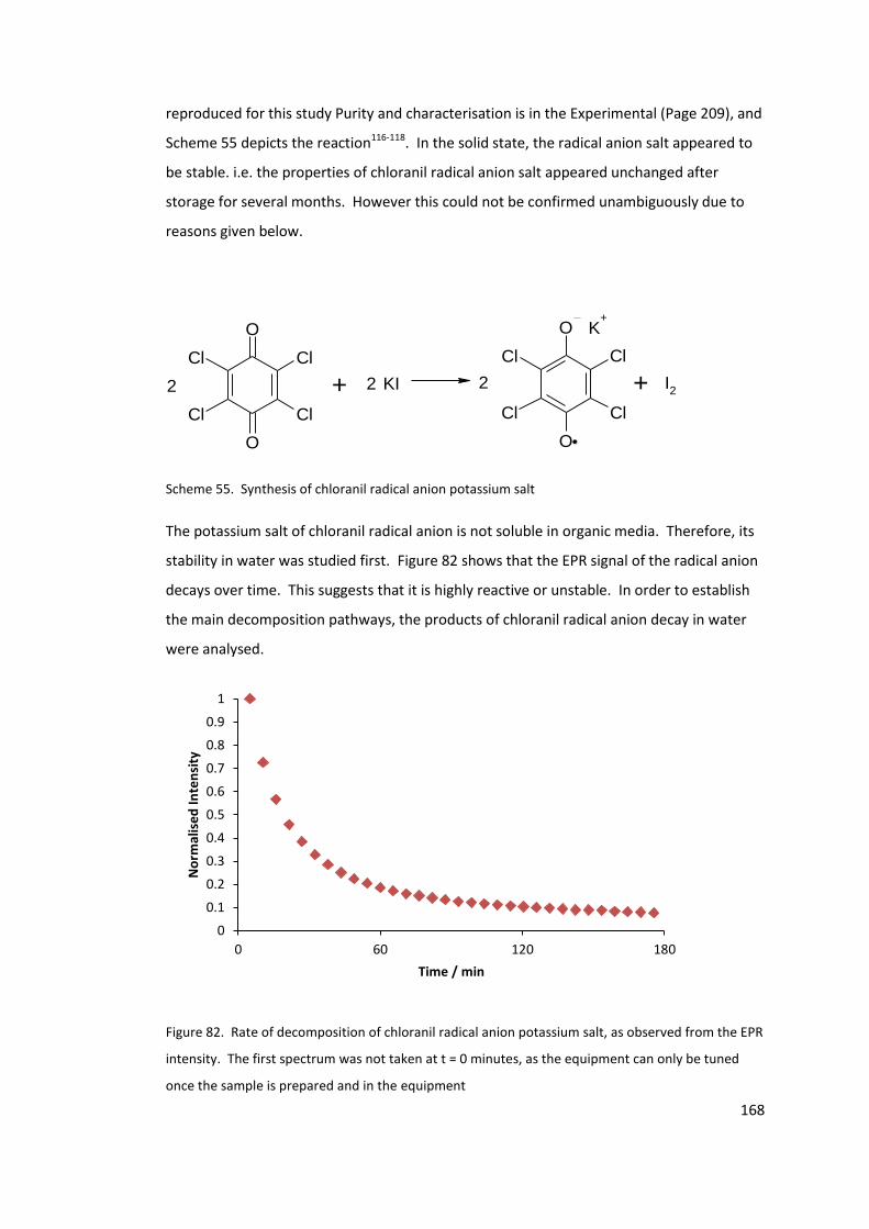
168
reproduced for this study Purity and characterisation is in the Experimental (Page 209), and
Scheme 55 depicts the reaction116-118. In the solid state, the radical anion salt appeared to
be stable. i.e. the properties of chloranil radical anion salt appeared unchanged after
storage for several months. However this could not be confirmed unambiguously due to
reasons given below.
O
O
Cl
ClCl
Cl
O
O
Cl
ClCl
Cl
KI I2
K+
2+2 2 +
Scheme 55. Synthesis of chloranil radical anion potassium salt
The potassium salt of chloranil radical anion is not soluble in organic media. Therefore, its
stability in water was studied first. Figure 82 shows that the EPR signal of the radical anion
decays over time. This suggests that it is highly reactive or unstable. In order to establish
the main decomposition pathways, the products of chloranil radical anion decay in water
were analysed.
Figure 82. Rate of decomposition of chloranil radical anion potassium salt, as observed from the EPR
intensity. The first spectrum was not taken at t = 0 minutes, as the equipment can only be tuned
once the sample is prepared and in the equipment
0
0.1
0.2
0.3
0.4
0.5
0.6
0.7
0.8
0.9
1
0 60 120 180
No
rmal
ise
d In
ten
sity
Time / min

169
5.2.1 Products from the decomposition of chloranil radical
anion potassium salt.
A 100 ppm solution of chloranil radical anion potassium salt in water was left until no EPR
signal was observable and was then subjected to negative ion ESI MS. A number of species
were observed that gave distinct isotope patterns. These patterns could be assigned to
chlorine containing compounds, and specifically the number of chlorine atoms in the
compounds could be determined.
Figure 83 shows the ESI MS spectrum obtained, labelled with proposed structures given in
Table 8. These structures are based on molecular formulas obtained by fitting the
experimental isotope patterns to the calculated ones and are the likely products formed.
As an example, the isotope pattern for the product at m/z 224 (peak A) is shown in Figure
84 in blue, with a calculated isotope pattern for comparison in red.
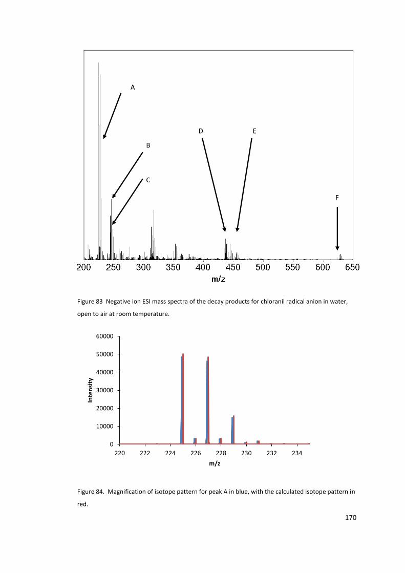
170
Figure 83 Negative ion ESI mass spectra of the decay products for chloranil radical anion in water,
open to air at room temperature.
Figure 84. Magnification of isotope pattern for peak A in blue, with the calculated isotope pattern in
red.
0
10000
20000
30000
40000
50000
60000
220 222 224 226 228 230 232 234
Inte
nsi
ty
m/z
B
C
D E
F
A
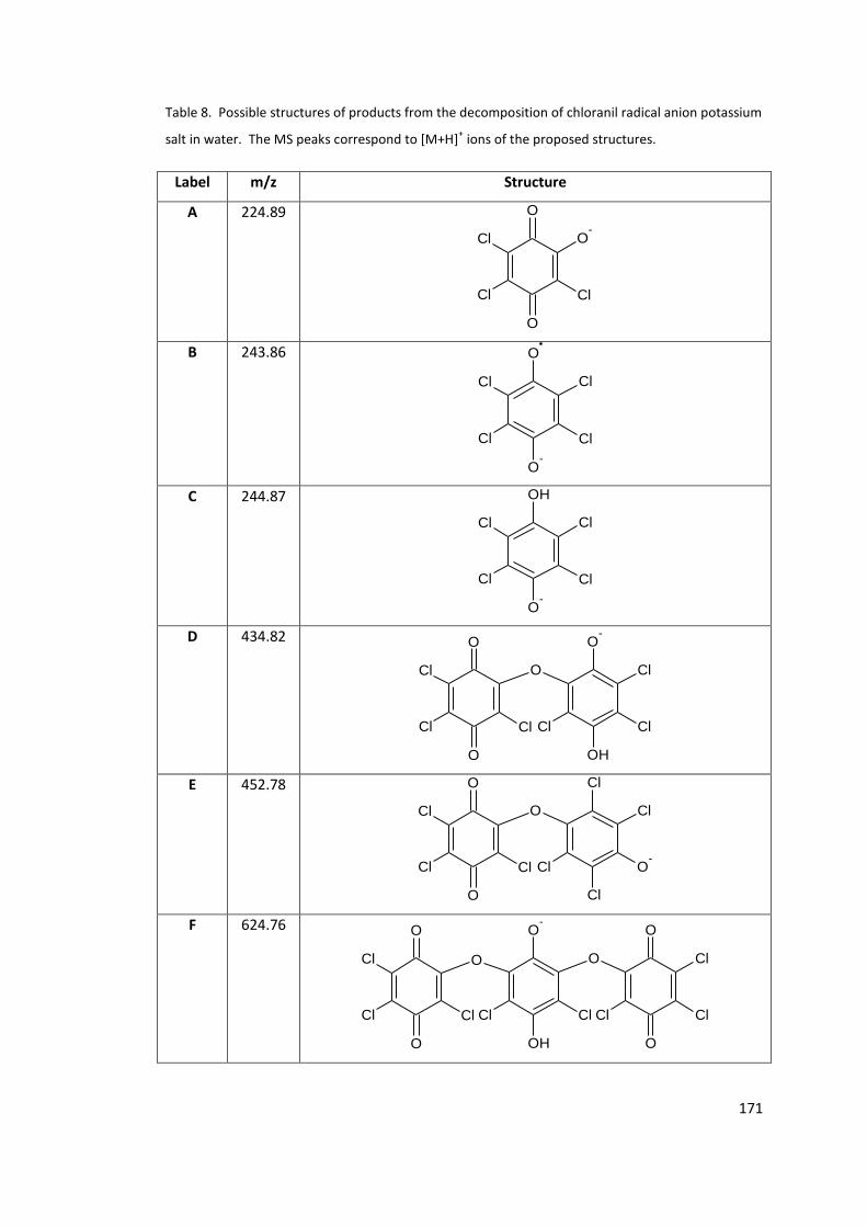
171
Table 8. Possible structures of products from the decomposition of chloranil radical anion potassium
salt in water. The MS peaks correspond to [M+H]+ ions of the proposed structures.
Label m/z Structure
A 224.89
O
O
Cl
Cl
O-
Cl
B 243.86 O
O-
Cl
Cl
Cl
Cl
C 244.87 OH
O-
Cl
Cl
Cl
Cl
D 434.82
O
O
O
Cl
O-
OH
Cl
Cl
Cl
Cl
Cl
E 452.78
O
O
O
Cl
Cl
Cl
Cl
Cl
O-
Cl
Cl
F 624.76
O O
Cl Cl Cl Cl
O
O
O
O
Cl
Cl
OH
O-
Cl
Cl
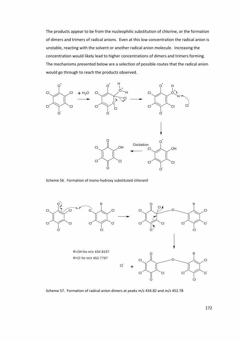
172
The products appear to be from the nucleophilic substitution of chlorine, or the formation
of dimers and trimers of radical anions. Even at this low concentration the radical anion is
unstable, reacting with the solvent or another radical anion molecule. Increasing the
concentration would likely lead to higher concentrations of dimers and trimers forming.
The mechanisms presented below are a selection of possible routes that the radical anion
would go through to reach the products observed.
O
O-
Cl
Cl Cl
Cl
C-
O
O-
Cl
ClCl
Cl
O+
H
H
H2O
O
O-
Cl
Cl Cl
O+
H
H
O
O-
Cl
Cl Cl
OH
O
O
Cl
Cl Cl
OHOxidation
Cl-
+
Scheme 56. Formation of mono-hydroxy substituted chloranil
Scheme 57. Formation of radical anion dimers at peaks m/z 434.82 and m/z 452.78
Cl
Cl
Cl
Cl
O
O-
O
Cl
Cl
O-
R
Cl
Cl
Cl
O-
Cl
Cl Cl
O
O
O-
Cl
RCl
Cl
Cl
O-
Cl
Cl Cl
O
O
O Cl
RR=OH for m/z 434.8157
R=Cl for m/z 452.7797
+Cl-
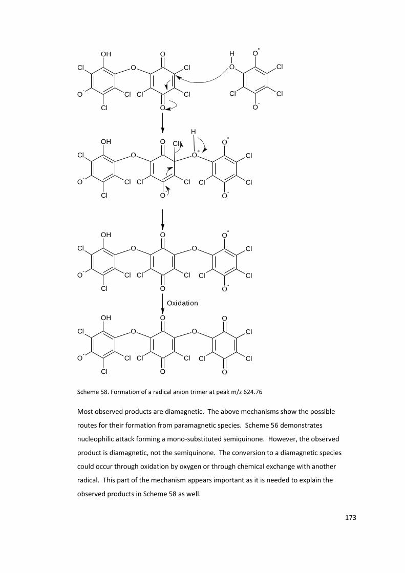
173
Scheme 58. Formation of a radical anion trimer at peak m/z 624.76
Most observed products are diamagnetic. The above mechanisms show the possible
routes for their formation from paramagnetic species. Scheme 56 demonstrates
nucleophilic attack forming a mono-substituted semiquinone. However, the observed
product is diamagnetic, not the semiquinone. The conversion to a diamagnetic species
could occur through oxidation by oxygen or through chemical exchange with another
radical. This part of the mechanism appears important as it is needed to explain the
observed products in Scheme 58 as well.
O
OH
Cl
O-
Cl
Cl Cl
O
O
Cl
Cl
O
O-
Cl
Cl
Cl
O
H
O
OH
Cl
O-
Cl
Cl Cl
O
O-
Cl
O+
H
O
Cl
Cl
O-
Cl
Cl
O
OH
Cl
O-
Cl
Cl Cl
O
O
Cl
O
O
Cl
Cl
O-
Cl
O
OH
Cl
O-
Cl
Cl Cl
O
O
Cl
O
O
Cl
Cl
O
Cl
Oxidation
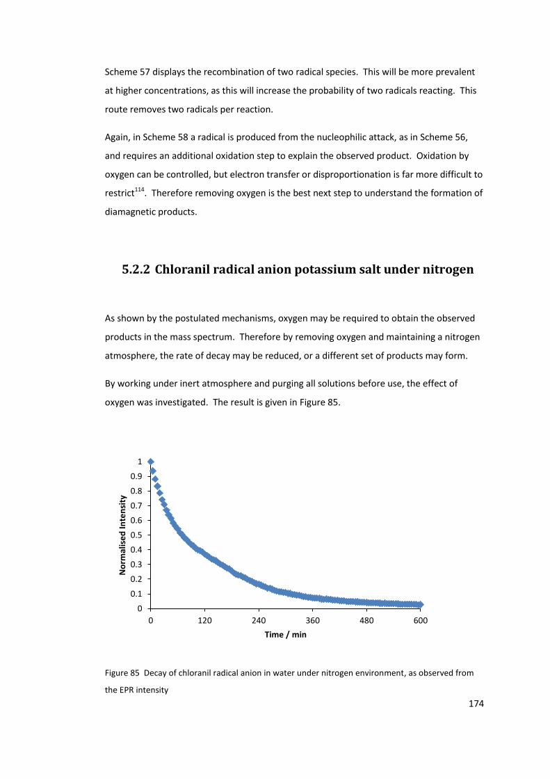
174
Scheme 57 displays the recombination of two radical species. This will be more prevalent
at higher concentrations, as this will increase the probability of two radicals reacting. This
route removes two radicals per reaction.
Again, in Scheme 58 a radical is produced from the nucleophilic attack, as in Scheme 56,
and requires an additional oxidation step to explain the observed product. Oxidation by
oxygen can be controlled, but electron transfer or disproportionation is far more difficult to
restrict114. Therefore removing oxygen is the best next step to understand the formation of
diamagnetic products.
5.2.2 Chloranil radical anion potassium salt under nitrogen
As shown by the postulated mechanisms, oxygen may be required to obtain the observed
products in the mass spectrum. Therefore by removing oxygen and maintaining a nitrogen
atmosphere, the rate of decay may be reduced, or a different set of products may form.
By working under inert atmosphere and purging all solutions before use, the effect of
oxygen was investigated. The result is given in Figure 85.
Figure 85 Decay of chloranil radical anion in water under nitrogen environment, as observed from
the EPR intensity
0
0.1
0.2
0.3
0.4
0.5
0.6
0.7
0.8
0.9
1
0 120 240 360 480 600
No
rmal
ise
d In
ten
sity
Time / min
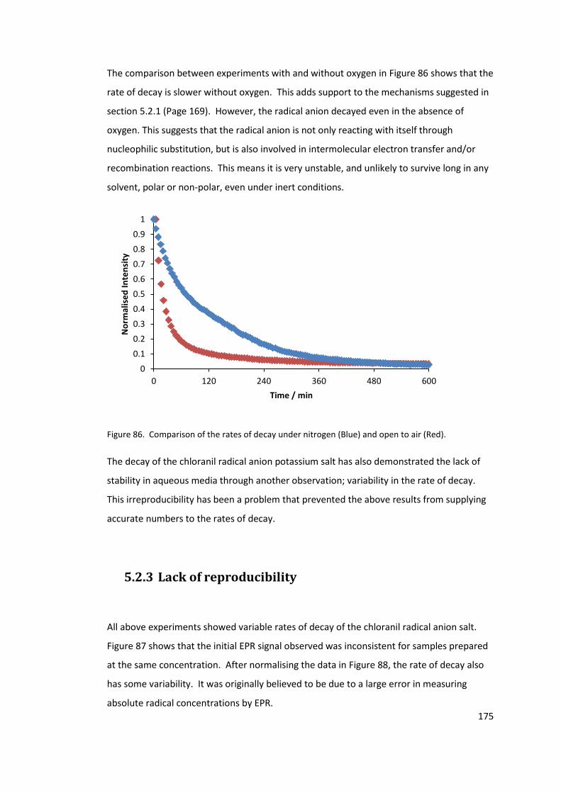
175
The comparison between experiments with and without oxygen in Figure 86 shows that the
rate of decay is slower without oxygen. This adds support to the mechanisms suggested in
section 5.2.1 (Page 169). However, the radical anion decayed even in the absence of
oxygen. This suggests that the radical anion is not only reacting with itself through
nucleophilic substitution, but is also involved in intermolecular electron transfer and/or
recombination reactions. This means it is very unstable, and unlikely to survive long in any
solvent, polar or non-polar, even under inert conditions.
Figure 86. Comparison of the rates of decay under nitrogen (Blue) and open to air (Red).
The decay of the chloranil radical anion potassium salt has also demonstrated the lack of
stability in aqueous media through another observation; variability in the rate of decay.
This irreproducibility has been a problem that prevented the above results from supplying
accurate numbers to the rates of decay.
5.2.3 Lack of reproducibility
All above experiments showed variable rates of decay of the chloranil radical anion salt.
Figure 87 shows that the initial EPR signal observed was inconsistent for samples prepared
at the same concentration. After normalising the data in Figure 88, the rate of decay also
has some variability. It was originally believed to be due to a large error in measuring
absolute radical concentrations by EPR.
0
0.1
0.2
0.3
0.4
0.5
0.6
0.7
0.8
0.9
1
0 120 240 360 480 600
No
rmal
ise
d In
ten
sity
Time / min
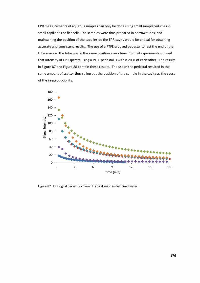
176
EPR measurements of aqueous samples can only be done using small sample volumes in
small capillaries or flat cells. The samples were thus prepared in narrow tubes, and
maintaining the position of the tube inside the EPR cavity would be critical for obtaining
accurate and consistent results. The use of a PTFE grooved pedestal to rest the end of the
tube ensured the tube was in the same position every time. Control experiments showed
that intensity of EPR spectra using a PTFE pedestal is within 20 % of each other. The results
in Figure 87 and Figure 88 contain these results. The use of the pedestal resulted in the
same amount of scatter thus ruling out the position of the sample in the cavity as the cause
of the irreproducibility.
Figure 87. EPR signal decay for chloranil radical anion in deionised water.
0
20
40
60
80
100
120
140
160
180
0 30 60 90 120 150 180
Sign
al in
ten
sity
Time (min)
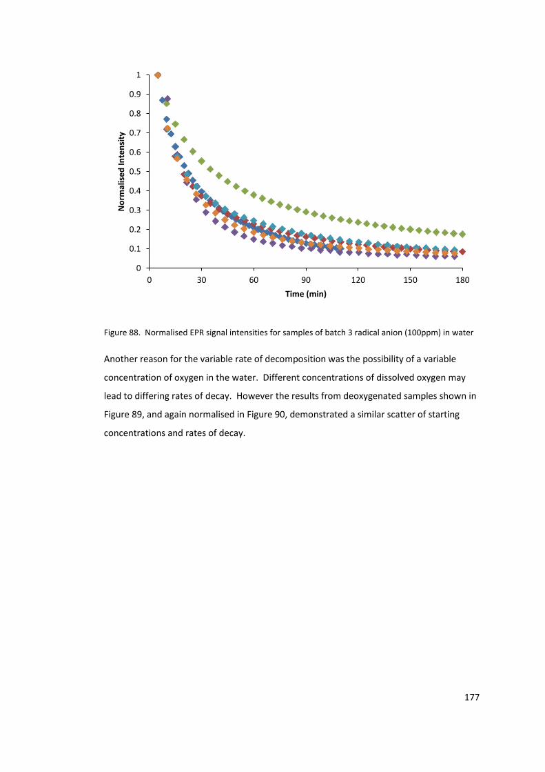
177
Figure 88. Normalised EPR signal intensities for samples of batch 3 radical anion (100ppm) in water
Another reason for the variable rate of decomposition was the possibility of a variable
concentration of oxygen in the water. Different concentrations of dissolved oxygen may
lead to differing rates of decay. However the results from deoxygenated samples shown in
Figure 89, and again normalised in Figure 90, demonstrated a similar scatter of starting
concentrations and rates of decay.
0
0.1
0.2
0.3
0.4
0.5
0.6
0.7
0.8
0.9
1
0 30 60 90 120 150 180
No
rmal
ise
d In
ten
sity
Time (min)
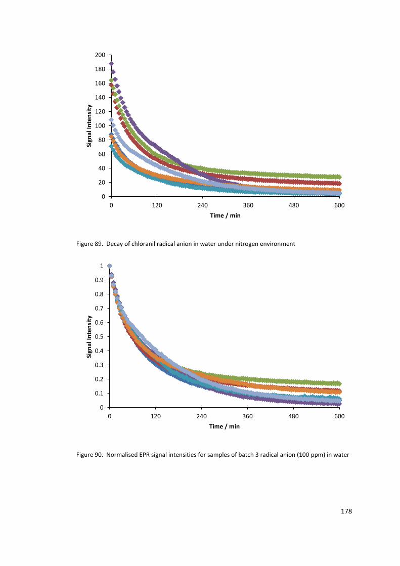
178
Figure 89. Decay of chloranil radical anion in water under nitrogen environment
Figure 90. Normalised EPR signal intensities for samples of batch 3 radical anion (100 ppm) in water
0
20
40
60
80
100
120
140
160
180
200
0 120 240 360 480 600
Sign
al I
nte
nsi
ty
Time / min
0
0.1
0.2
0.3
0.4
0.5
0.6
0.7
0.8
0.9
1
0 120 240 360 480 600
Sign
al I
nte
nsi
ty
Time / min
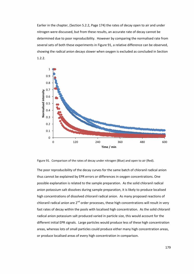
179
Earlier in the chapter, (Section 5.2.2, Page 174) the rates of decay open to air and under
nitrogen were discussed, but from these results, an accurate rate of decay cannot be
determined due to poor reproducibility. However by comparing the normalised rate from
several sets of both these experiments in Figure 91, a relative difference can be observed,
showing the radical anion decays slower when oxygen is excluded as concluded in Section
1.2.2.
Figure 91. Comparison of the rates of decay under nitrogen (Blue) and open to air (Red).
The poor reproducibility of the decay curves for the same batch of chloranil radical anion
thus cannot be explained by EPR errors or differences in oxygen concentrations. One
possible explanation is related to the sample preparation. As the solid chloranil radical
anion potassium salt dissolves during sample preparation, it is likely to produce localised
high concentrations of dissolved chloranil radical anion. As many proposed reactions of
chloranil radical anion are 2nd order processes, these high concentrations will result in very
fast rates of decay within the pools with localised high concentration. As the solid chloranil
radical anion potassium salt produced varied in particle size, this would account for the
different initial EPR signals. Large particles would produce less of these high concentration
areas, whereas lots of small particles could produce either many high concentration areas,
or produce localised areas of every high concentration in comparison.
0
0.1
0.2
0.3
0.4
0.5
0.6
0.7
0.8
0.9
1
0 120 240 360 480 600
No
rmal
ise
d in
ten
sity
Time / min

180
This theory was not investigated further, as maintaining a consistent rate of dissolution is a
challenging task which goes beyond the scope of this thesis.
5.2.4 Conclusions
It is difficult to make solid conclusions from the above work due to the lack of
reproducibility in results. The fact that rates of chloranil radical anion decay are not
reproducible suggests that it is unstable in water. Its stability is unknown in organic media
due to the lack of solubility of the salt in those solvents. The lack of reproducibility could
be due to high localised concentrations of the radical anion temporarily formed during its
dissolution in water. The poor stability of the radical anion leads to a mixture of
nucleophilic substitutions, oxidations and disproportionations.
In terms of polymerisation inhibition, lack of solubility in organic solvents limits which
monomers it can protect. However, it is unlikely to be used in its potassium salt form.
It has been shown that the rate of decay in water is slower without oxygen but still
significant. From this observation and the products observed, it can be suggested that the
main route of decay is from the radical anion reacting with itself. This does not bode well
for the radical anion being used as a polymerisation inhibitor. Compounds used as storage
inhibitors need to survive for a long time to be of any use at protecting the monomer from
polymerising
The initial EPR signal obtained from the chloranil radical anion potassium salt dissolved in
water never depicted the expected concentration of radicals in solution. The maximum
concentration of radical observed was 70% of the salt dissolved, with the average around
50%. This suggests that the radical anion immediately decays or reacts into non radical
components. One possibility is that the radical anion disproportionates to give chloranil
and tetrachloro hydroquinone dianion. This in turn would establish a comproportionation /
disproportionation equilibrium, and understanding the position the equilibrium lies may
offer some explanation for the observed discrepancy.
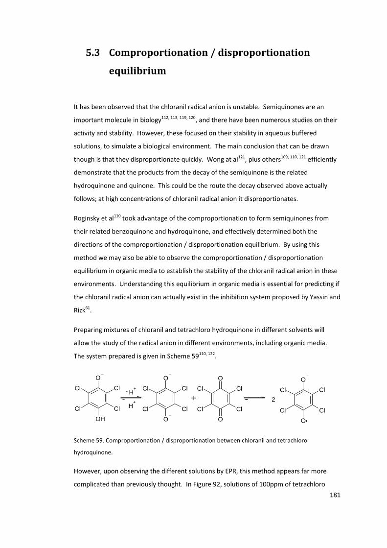
181
5.3 Comproportionation / disproportionation
equilibrium
It has been observed that the chloranil radical anion is unstable. Semiquinones are an
important molecule in biology112, 113, 119, 120, and there have been numerous studies on their
activity and stability. However, these focused on their stability in aqueous buffered
solutions, to simulate a biological environment. The main conclusion that can be drawn
though is that they disproportionate quickly. Wong at al121, plus others109, 110, 121 efficiently
demonstrate that the products from the decay of the semiquinone is the related
hydroquinone and quinone. This could be the route the decay observed above actually
follows; at high concentrations of chloranil radical anion it disproportionates.
Roginsky et al110 took advantage of the comproportionation to form semiquinones from
their related benzoquinone and hydroquinone, and effectively determined both the
directions of the comproportionation / disproportionation equilibrium. By using this
method we may also be able to observe the comproportionation / disproportionation
equilibrium in organic media to establish the stability of the chloranil radical anion in these
environments. Understanding this equilibrium in organic media is essential for predicting if
the chloranil radical anion can actually exist in the inhibition system proposed by Yassin and
Rizk61.
Preparing mixtures of chloranil and tetrachloro hydroquinone in different solvents will
allow the study of the radical anion in different environments, including organic media.
The system prepared is given in Scheme 59110, 122.
O
O
Cl
ClCl
Cl
O
O
Cl
ClCl
Cl
O
O
Cl
ClCl
Cl
O
OH
Cl
ClCl
Cl H+
H+
+-
2
Scheme 59. Comproportionation / disproportionation between chloranil and tetrachloro
hydroquinone.
However, upon observing the different solutions by EPR, this method appears far more
complicated than previously thought. In Figure 92, solutions of 100ppm of tetrachloro
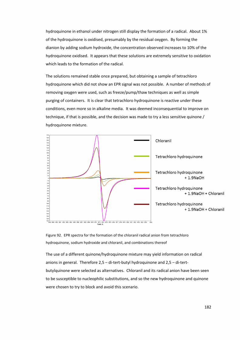
182
hydroquinone in ethanol under nitrogen still display the formation of a radical. About 1%
of the hydroquinone is oxidised, presumably by the residual oxygen. By forming the
dianion by adding sodium hydroxide, the concentration observed increases to 10% of the
hydroquinone oxidised. It appears that these solutions are extremely sensitive to oxidation
which leads to the formation of the radical.
The solutions remained stable once prepared, but obtaining a sample of tetrachloro
hydroquinone which did not show an EPR signal was not possible. A number of methods of
removing oxygen were used, such as freeze/pump/thaw techniques as well as simple
purging of containers. It is clear that tetrachloro hydroquinone is reactive under these
conditions, even more so in alkaline media. It was deemed inconsequential to improve on
technique, if that is possible, and the decision was made to try a less sensitive quinone /
hydroquinone mixture.
Figure 92. EPR spectra for the formation of the chloranil radical anion from tetrachloro
hydroquinone, sodium hydroxide and chloranil, and combinations thereof
The use of a different quinone/hydroquinone mixture may yield information on radical
anions in general. Therefore 2,5 – di-tert-butyl hydroquinone and 2,5 – di-tert-
butylquinone were selected as alternatives. Chloranil and its radical anion have been seen
to be susceptible to nucleophilic substitutions, and so the new hydroquinone and quinone
were chosen to try to block and avoid this scenario.
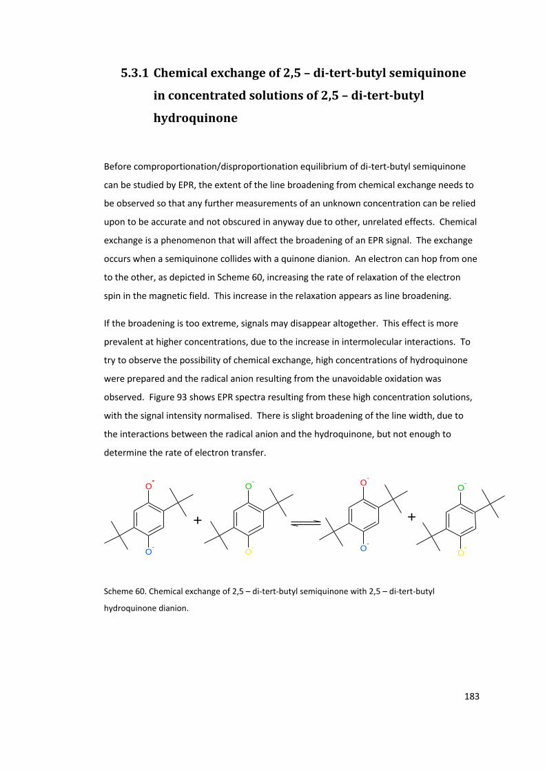
183
5.3.1 Chemical exchange of 2,5 – di-tert-butyl semiquinone
in concentrated solutions of 2,5 – di-tert-butyl
hydroquinone
Before comproportionation/disproportionation equilibrium of di-tert-butyl semiquinone
can be studied by EPR, the extent of the line broadening from chemical exchange needs to
be observed so that any further measurements of an unknown concentration can be relied
upon to be accurate and not obscured in anyway due to other, unrelated effects. Chemical
exchange is a phenomenon that will affect the broadening of an EPR signal. The exchange
occurs when a semiquinone collides with a quinone dianion. An electron can hop from one
to the other, as depicted in Scheme 60, increasing the rate of relaxation of the electron
spin in the magnetic field. This increase in the relaxation appears as line broadening.
If the broadening is too extreme, signals may disappear altogether. This effect is more
prevalent at higher concentrations, due to the increase in intermolecular interactions. To
try to observe the possibility of chemical exchange, high concentrations of hydroquinone
were prepared and the radical anion resulting from the unavoidable oxidation was
observed. Figure 93 shows EPR spectra resulting from these high concentration solutions,
with the signal intensity normalised. There is slight broadening of the line width, due to
the interactions between the radical anion and the hydroquinone, but not enough to
determine the rate of electron transfer.
O
O-
O-
O
O-
O-
+
O-
O-
+
Scheme 60. Chemical exchange of 2,5 – di-tert-butyl semiquinone with 2,5 – di-tert-butyl
hydroquinone dianion.
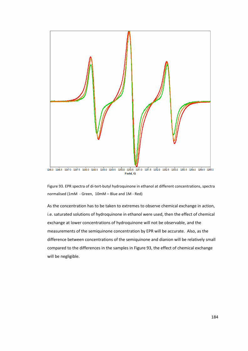
184
Figure 93. EPR spectra of di-tert-butyl hydroquinone in ethanol at different concentrations, spectra
normalised (1mM - Green, 10mM – Blue and 1M - Red)
As the concentration has to be taken to extremes to observe chemical exchange in action,
i.e. saturated solutions of hydroquinone in ethanol were used, then the effect of chemical
exchange at lower concentrations of hydroquinone will not be observable, and the
measurements of the semiquinone concentration by EPR will be accurate. Also, as the
difference between concentrations of the semiquinone and dianion will be relatively small
compared to the differences in the samples in Figure 93, the effect of chemical exchange
will be negligible.
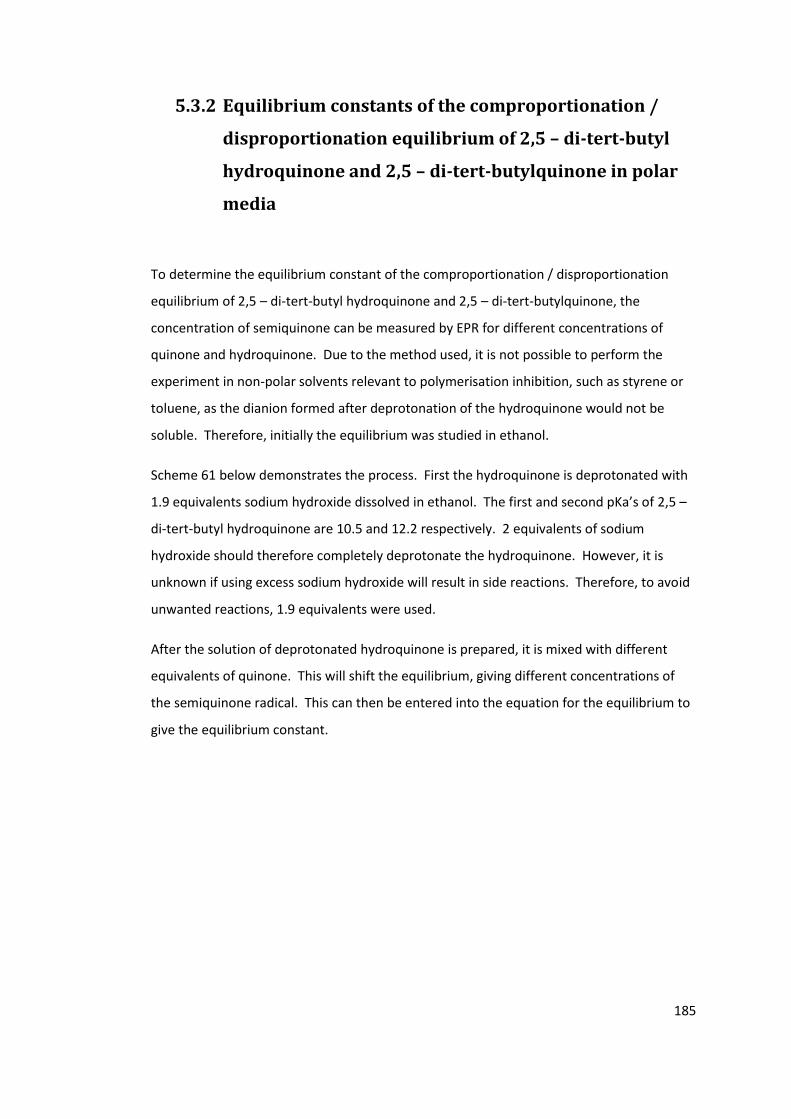
185
5.3.2 Equilibrium constants of the comproportionation /
disproportionation equilibrium of 2,5 – di-tert-butyl
hydroquinone and 2,5 – di-tert-butylquinone in polar
media
To determine the equilibrium constant of the comproportionation / disproportionation
equilibrium of 2,5 – di-tert-butyl hydroquinone and 2,5 – di-tert-butylquinone, the
concentration of semiquinone can be measured by EPR for different concentrations of
quinone and hydroquinone. Due to the method used, it is not possible to perform the
experiment in non-polar solvents relevant to polymerisation inhibition, such as styrene or
toluene, as the dianion formed after deprotonation of the hydroquinone would not be
soluble. Therefore, initially the equilibrium was studied in ethanol.
Scheme 61 below demonstrates the process. First the hydroquinone is deprotonated with
1.9 equivalents sodium hydroxide dissolved in ethanol. The first and second pKa’s of 2,5 –
di-tert-butyl hydroquinone are 10.5 and 12.2 respectively. 2 equivalents of sodium
hydroxide should therefore completely deprotonate the hydroquinone. However, it is
unknown if using excess sodium hydroxide will result in side reactions. Therefore, to avoid
unwanted reactions, 1.9 equivalents were used.
After the solution of deprotonated hydroquinone is prepared, it is mixed with different
equivalents of quinone. This will shift the equilibrium, giving different concentrations of
the semiquinone radical. This can then be entered into the equation for the equilibrium to
give the equilibrium constant.
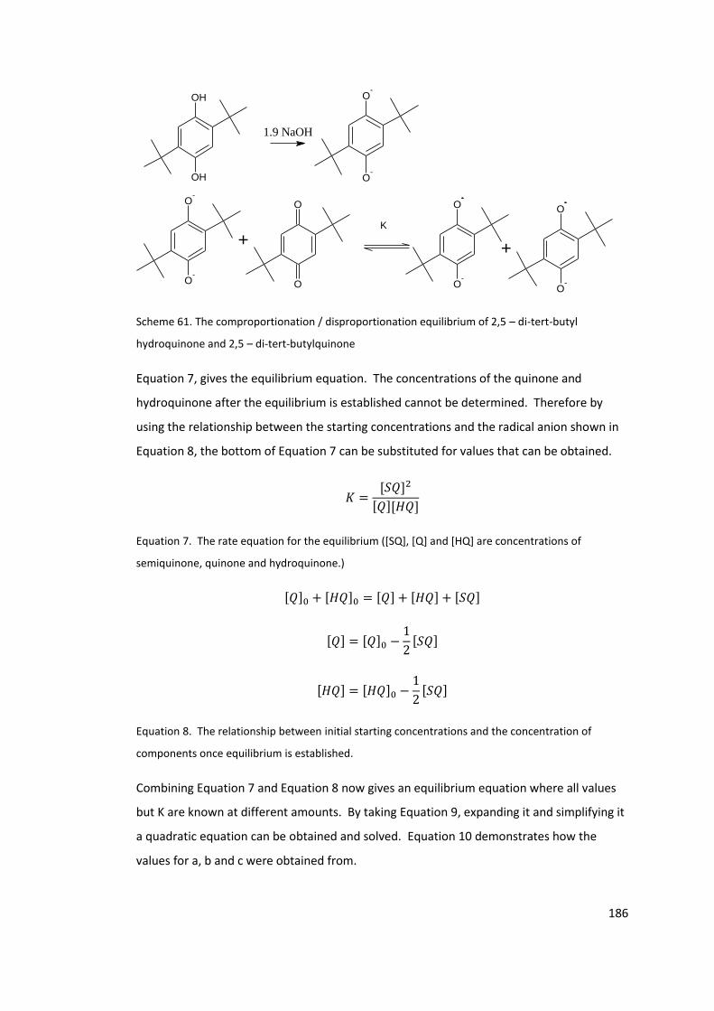
186
OH
OH
1.9 NaOH
O-
O-
O-
O-
+
O
O
O
O-
O
O-
+
K
Scheme 61. The comproportionation / disproportionation equilibrium of 2,5 – di-tert-butyl
hydroquinone and 2,5 – di-tert-butylquinone
Equation 7, gives the equilibrium equation. The concentrations of the quinone and
hydroquinone after the equilibrium is established cannot be determined. Therefore by
using the relationship between the starting concentrations and the radical anion shown in
Equation 8, the bottom of Equation 7 can be substituted for values that can be obtained.
𝐾 =[𝑆𝑄]2
[𝑄][𝐻𝑄]
Equation 7. The rate equation for the equilibrium ([SQ], [Q] and [HQ] are concentrations of
semiquinone, quinone and hydroquinone.)
[𝑄]0 + [𝐻𝑄]0 = [𝑄] + [𝐻𝑄] + [𝑆𝑄]
[𝑄] = [𝑄]0 −1
2[𝑆𝑄]
[𝐻𝑄] = [𝐻𝑄]0 −1
2[𝑆𝑄]
Equation 8. The relationship between initial starting concentrations and the concentration of
components once equilibrium is established.
Combining Equation 7 and Equation 8 now gives an equilibrium equation where all values
but K are known at different amounts. By taking Equation 9, expanding it and simplifying it
a quadratic equation can be obtained and solved. Equation 10 demonstrates how the
values for a, b and c were obtained from.
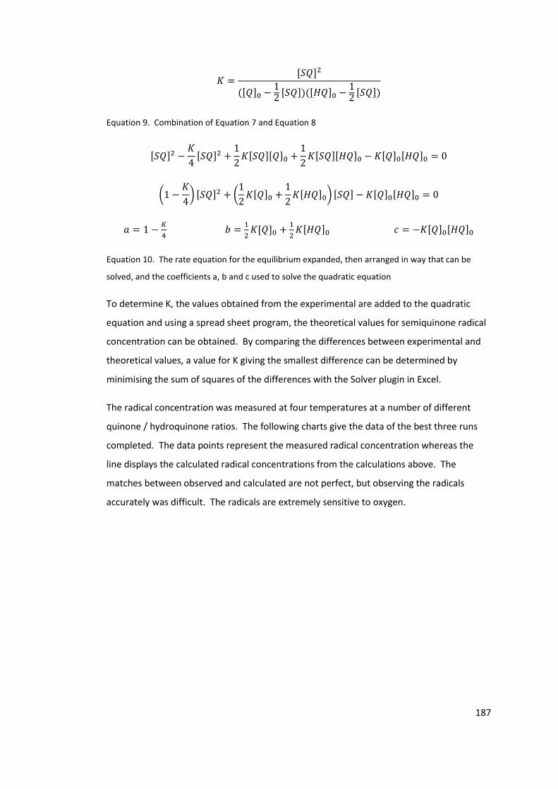
187
𝐾 =[𝑆𝑄]2
([𝑄]0 −12[𝑆𝑄])([𝐻𝑄]0 −
12[𝑆𝑄])
Equation 9. Combination of Equation 7 and Equation 8
[𝑆𝑄]2 −𝐾
4[𝑆𝑄]2 +
1
2𝐾[𝑆𝑄][𝑄]0 +
1
2𝐾[𝑆𝑄][𝐻𝑄]0 − 𝐾[𝑄]0[𝐻𝑄]0 = 0
(1 −𝐾
4) [𝑆𝑄]2 + (
1
2𝐾[𝑄]0 +
1
2𝐾[𝐻𝑄]0) [𝑆𝑄] − 𝐾[𝑄]0[𝐻𝑄]0 = 0
𝑎 = 1 −𝐾
4 𝑏 =
1
2𝐾[𝑄]0 +
1
2𝐾[𝐻𝑄]0 𝑐 = −𝐾[𝑄]0[𝐻𝑄]0
Equation 10. The rate equation for the equilibrium expanded, then arranged in way that can be
solved, and the coefficients a, b and c used to solve the quadratic equation
To determine K, the values obtained from the experimental are added to the quadratic
equation and using a spread sheet program, the theoretical values for semiquinone radical
concentration can be obtained. By comparing the differences between experimental and
theoretical values, a value for K giving the smallest difference can be determined by
minimising the sum of squares of the differences with the Solver plugin in Excel.
The radical concentration was measured at four temperatures at a number of different
quinone / hydroquinone ratios. The following charts give the data of the best three runs
completed. The data points represent the measured radical concentration whereas the
line displays the calculated radical concentrations from the calculations above. The
matches between observed and calculated are not perfect, but observing the radicals
accurately was difficult. The radicals are extremely sensitive to oxygen.
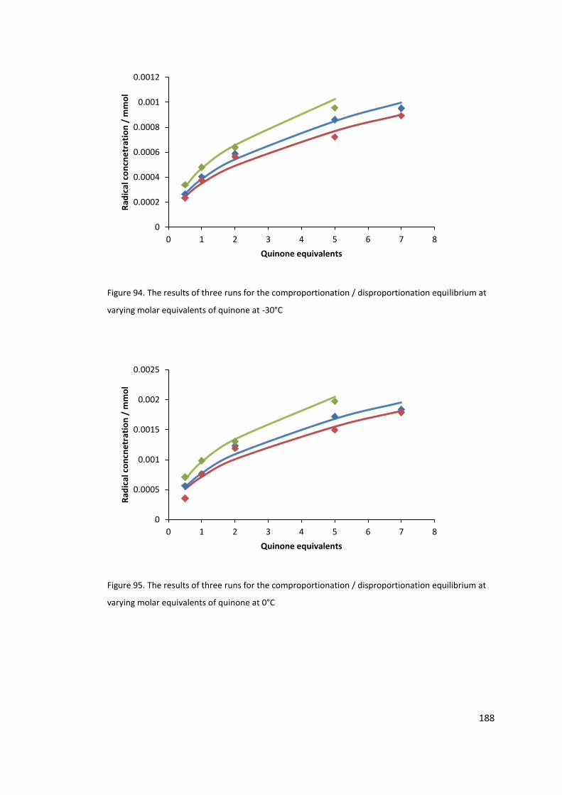
188
Figure 94. The results of three runs for the comproportionation / disproportionation equilibrium at
varying molar equivalents of quinone at -30°C
Figure 95. The results of three runs for the comproportionation / disproportionation equilibrium at
varying molar equivalents of quinone at 0°C
0
0.0002
0.0004
0.0006
0.0008
0.001
0.0012
0 1 2 3 4 5 6 7 8
Rad
ical
co
ncn
etr
atio
n /
mm
ol
Quinone equivalents
0
0.0005
0.001
0.0015
0.002
0.0025
0 1 2 3 4 5 6 7 8
Rad
ical
co
ncn
etr
atio
n /
mm
ol
Quinone equivalents
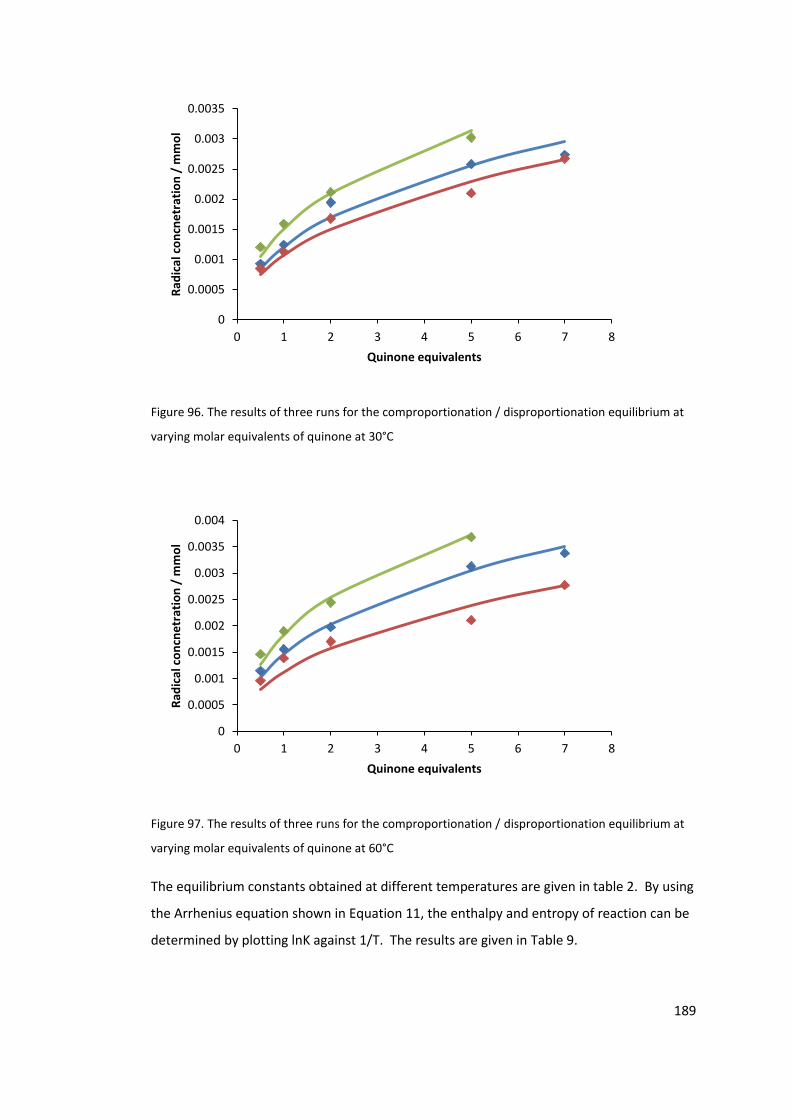
189
Figure 96. The results of three runs for the comproportionation / disproportionation equilibrium at
varying molar equivalents of quinone at 30°C
Figure 97. The results of three runs for the comproportionation / disproportionation equilibrium at
varying molar equivalents of quinone at 60°C
The equilibrium constants obtained at different temperatures are given in table 2. By using
the Arrhenius equation shown in Equation 11, the enthalpy and entropy of reaction can be
determined by plotting lnK against 1/T. The results are given in Table 9.
0
0.0005
0.001
0.0015
0.002
0.0025
0.003
0.0035
0 1 2 3 4 5 6 7 8
Rad
ical
co
ncn
etr
atio
n /
mm
ol
Quinone equivalents
0
0.0005
0.001
0.0015
0.002
0.0025
0.003
0.0035
0.004
0 1 2 3 4 5 6 7 8
Rad
ical
co
ncn
etr
atio
n /
mm
ol
Quinone equivalents
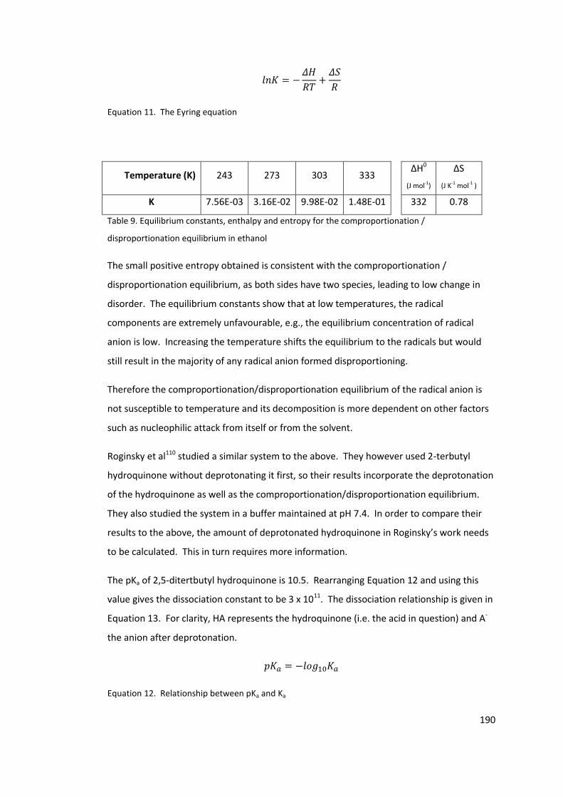
190
𝑙𝑛𝐾 = −𝛥𝐻
𝑅𝑇+𝛥𝑆
𝑅
Equation 11. The Eyring equation
Temperature (K) 243 273 303 333 ∆H0
(J mol-1)
∆S
(J K-1 mol-1 )
K 7.56E-03 3.16E-02 9.98E-02 1.48E-01 332 0.78
Table 9. Equilibrium constants, enthalpy and entropy for the comproportionation /
disproportionation equilibrium in ethanol
The small positive entropy obtained is consistent with the comproportionation /
disproportionation equilibrium, as both sides have two species, leading to low change in
disorder. The equilibrium constants show that at low temperatures, the radical
components are extremely unfavourable, e.g., the equilibrium concentration of radical
anion is low. Increasing the temperature shifts the equilibrium to the radicals but would
still result in the majority of any radical anion formed disproportioning.
Therefore the comproportionation/disproportionation equilibrium of the radical anion is
not susceptible to temperature and its decomposition is more dependent on other factors
such as nucleophilic attack from itself or from the solvent.
Roginsky et al110 studied a similar system to the above. They however used 2-terbutyl
hydroquinone without deprotonating it first, so their results incorporate the deprotonation
of the hydroquinone as well as the comproportionation/disproportionation equilibrium.
They also studied the system in a buffer maintained at pH 7.4. In order to compare their
results to the above, the amount of deprotonated hydroquinone in Roginsky’s work needs
to be calculated. This in turn requires more information.
The pKa of 2,5-ditertbutyl hydroquinone is 10.5. Rearranging Equation 12 and using this
value gives the dissociation constant to be 3 x 10¹¹. The dissociation relationship is given in
Equation 13. For clarity, HA represents the hydroquinone (i.e. the acid in question) and A-
the anion after deprotonation.
𝑝𝐾𝑎 = −𝑙𝑜𝑔10𝐾𝑎
Equation 12. Relationship between pKa and Ka
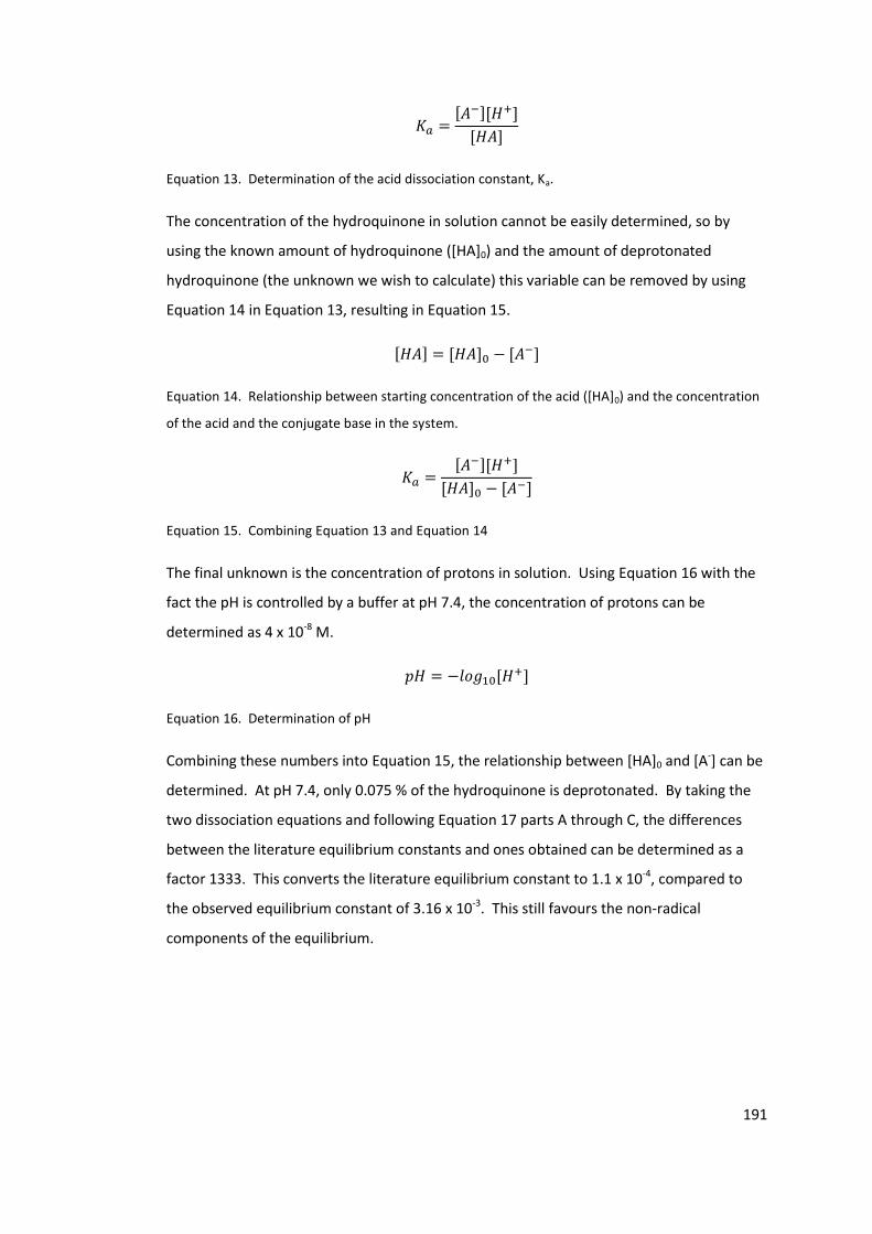
191
𝐾𝑎 =[𝐴−][𝐻+]
[𝐻𝐴]
Equation 13. Determination of the acid dissociation constant, Ka.
The concentration of the hydroquinone in solution cannot be easily determined, so by
using the known amount of hydroquinone ([HA]0) and the amount of deprotonated
hydroquinone (the unknown we wish to calculate) this variable can be removed by using
Equation 14 in Equation 13, resulting in Equation 15.
[𝐻𝐴] = [𝐻𝐴]0 − [𝐴−]
Equation 14. Relationship between starting concentration of the acid ([HA]0) and the concentration
of the acid and the conjugate base in the system.
𝐾𝑎 =[𝐴−][𝐻+]
[𝐻𝐴]0 − [𝐴−]
Equation 15. Combining Equation 13 and Equation 14
The final unknown is the concentration of protons in solution. Using Equation 16 with the
fact the pH is controlled by a buffer at pH 7.4, the concentration of protons can be
determined as 4 x 10⁻⁸ M.
𝑝𝐻 = −𝑙𝑜𝑔10[𝐻+]
Equation 16. Determination of pH
Combining these numbers into Equation 15, the relationship between [HA]0 and [A-] can be
determined. At pH 7.4, only 0.075 % of the hydroquinone is deprotonated. By taking the
two dissociation equations and following Equation 17 parts A through C, the differences
between the literature equilibrium constants and ones obtained can be determined as a
factor 1333. This converts the literature equilibrium constant to 1.1 x 10⁻⁴, compared to
the observed equilibrium constant of 3.16 x 10⁻³. This still favours the non-radical
components of the equilibrium.
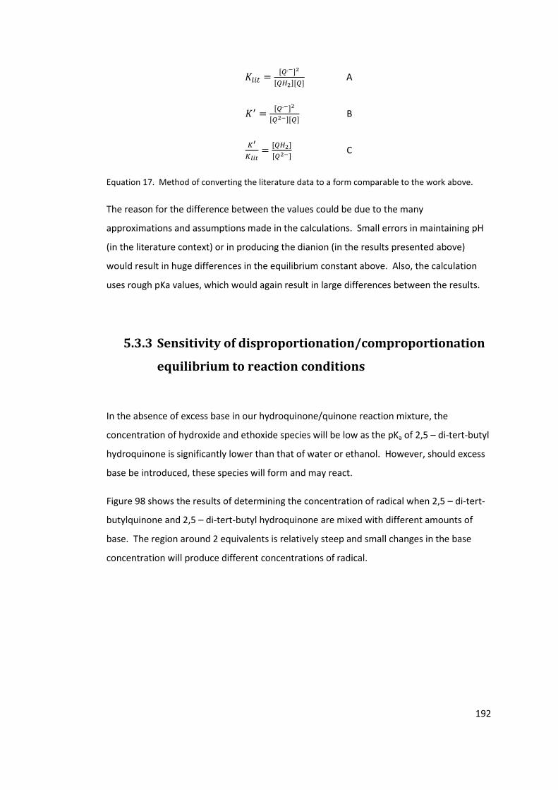
192
𝐾𝑙𝑖𝑡 =[𝑄.−]2
[𝑄𝐻2][𝑄] A
𝐾′ =[𝑄.−]2
[𝑄2−][𝑄] B
𝐾′
𝐾𝑙𝑖𝑡=[𝑄𝐻2]
[𝑄2−] C
Equation 17. Method of converting the literature data to a form comparable to the work above.
The reason for the difference between the values could be due to the many
approximations and assumptions made in the calculations. Small errors in maintaining pH
(in the literature context) or in producing the dianion (in the results presented above)
would result in huge differences in the equilibrium constant above. Also, the calculation
uses rough pKa values, which would again result in large differences between the results.
5.3.3 Sensitivity of disproportionation/comproportionation
equilibrium to reaction conditions
In the absence of excess base in our hydroquinone/quinone reaction mixture, the
concentration of hydroxide and ethoxide species will be low as the pKa of 2,5 – di-tert-butyl
hydroquinone is significantly lower than that of water or ethanol. However, should excess
base be introduced, these species will form and may react.
Figure 98 shows the results of determining the concentration of radical when 2,5 – di-tert-
butylquinone and 2,5 – di-tert-butyl hydroquinone are mixed with different amounts of
base. The region around 2 equivalents is relatively steep and small changes in the base
concentration will produce different concentrations of radical.
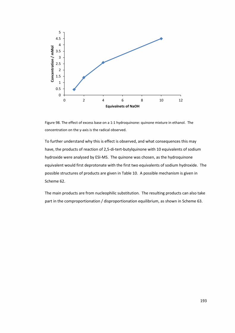
193
Figure 98. The effect of excess base on a 1:1 hydroquinone: quinone mixture in ethanol. The
concentration on the y-axis is the radical observed.
To further understand why this is effect is observed, and what consequences this may
have, the products of reaction of 2,5-di-tert-butylquinone with 10 equivalents of sodium
hydroxide were analysed by ESI-MS. The quinone was chosen, as the hydroquinone
equivalent would first deprotonate with the first two equivalents of sodium hydroxide. The
possible structures of products are given in Table 10. A possible mechanism is given in
Scheme 62.
The main products are from nucleophilic substitution. The resulting products can also take
part in the comproportionation / disproportionation equilibrium, as shown in Scheme 63.
0
0.5
1
1.5
2
2.5
3
3.5
4
4.5
5
0 2 4 6 8 10 12
Co
nce
ntr
atio
n /
mM
ol
Equivalnets of NaOH

194
Observed mass Possible structure Formula Calculated mass
237.15
OH
O-
C14H21O3 237.149
253.14
OH
O-
OH
OH
C14H21O4 253.146
281.16
OH
O-
O
OH
C16H25O4 281.175
Table 10. Structures for possible products for the decomposition of quinone in base
O
O
H
R
O-
O
H
R
OH-
O-
O-
R
OHH
OH
O-
R
Scheme 62. A possible mechanism for the formation of mono substituted product observed in the
reaction between the quinone and excess base.
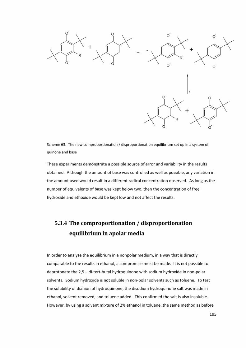
195
O-
O-
R
O
O
+
O
O
R
O-
O-
+
O
O-
R
O
O-
+
Scheme 63. The new comproportionation / disproportionation equilibrium set up in a system of
quinone and base
These experiments demonstrate a possible source of error and variability in the results
obtained. Although the amount of base was controlled as well as possible, any variation in
the amount used would result in a different radical concentration observed. As long as the
number of equivalents of base was kept below two, then the concentration of free
hydroxide and ethoxide would be kept low and not affect the results.
5.3.4 The comproportionation / disproportionation
equilibrium in apolar media
In order to analyse the equilibrium in a nonpolar medium, in a way that is directly
comparable to the results in ethanol, a compromise must be made. It is not possible to
deprotonate the 2,5 – di-tert-butyl hydroquinone with sodium hydroxide in non-polar
solvents. Sodium hydroxide is not soluble in non-polar solvents such as toluene. To test
the solubility of dianion of hydroquinone, the disodium hydroquinone salt was made in
ethanol, solvent removed, and toluene added. This confirmed the salt is also insoluble.
However, by using a solvent mixture of 2% ethanol in toluene, the same method as before
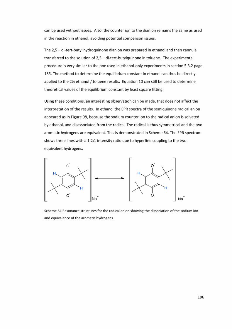
196
can be used without issues. Also, the counter ion to the dianion remains the same as used
in the reaction in ethanol, avoiding potential comparison issues.
The 2,5 – di-tert-butyl hydroquinone dianion was prepared in ethanol and then cannula
transferred to the solution of 2,5 – di-tert-butylquinone in toluene. The experimental
procedure is very similar to the one used in ethanol-only experiments in section 5.3.2 page
185. The method to determine the equilibrium constant in ethanol can thus be directly
applied to the 2% ethanol / toluene results. Equation 10 can still be used to determine
theoretical values of the equilibrium constant by least square fitting.
Using these conditions, an interesting observation can be made, that does not affect the
interpretation of the results. In ethanol the EPR spectra of the semiquinone radical anion
appeared as in Figure 98, because the sodium counter ion to the radical anion is solvated
by ethanol, and disassociated from the radical. The radical is thus symmetrical and the two
aromatic hydrogens are equivalent. This is demonstrated in Scheme 64. The EPR spectrum
shows three lines with a 1:2:1 intensity ratio due to hyperfine coupling to the two
equivalent hydrogens.
O
O-
H
H
O-
O
H
H
Na+
Na+
Scheme 64 Resonance structures for the radical anion showing the dissociation of the sodium ion
and equivalence of the aromatic hydrogens.
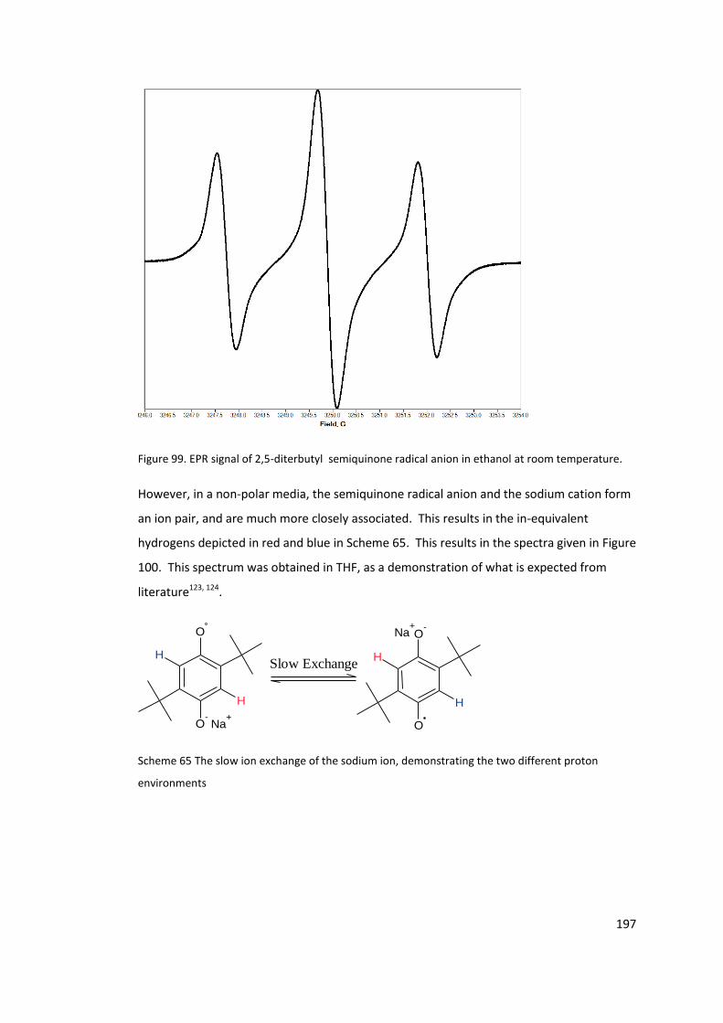
197
Figure 99. EPR signal of 2,5-diterbutyl semiquinone radical anion in ethanol at room temperature.
However, in a non-polar media, the semiquinone radical anion and the sodium cation form
an ion pair, and are much more closely associated. This results in the in-equivalent
hydrogens depicted in red and blue in Scheme 65. This results in the spectra given in Figure
100. This spectrum was obtained in THF, as a demonstration of what is expected from
literature123, 124.
O
O-
H
H
O-
O
H
H
Na+
Na+
Slow Exchange
Scheme 65 The slow ion exchange of the sodium ion, demonstrating the two different proton
environments
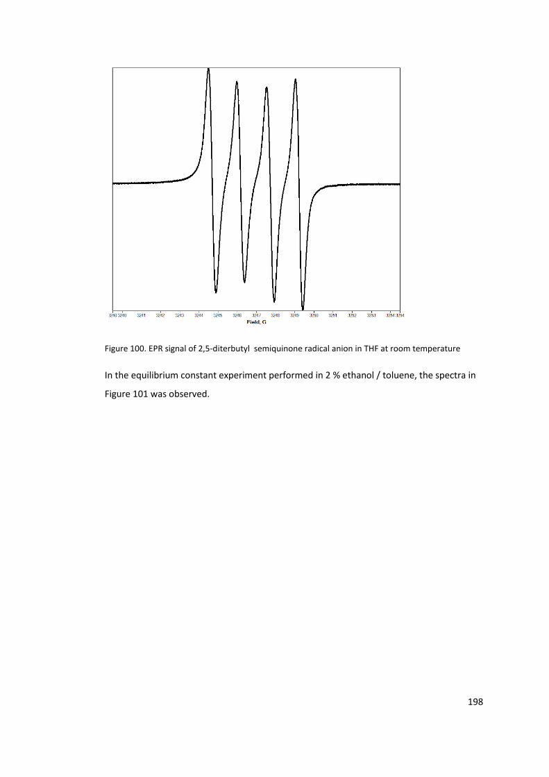
198
Figure 100. EPR signal of 2,5-diterbutyl semiquinone radical anion in THF at room temperature
In the equilibrium constant experiment performed in 2 % ethanol / toluene, the spectra in
Figure 101 was observed.
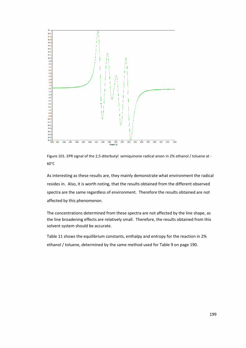
199
Figure 101. EPR signal of the 2,5-diterbutyl semiquinone radical anion in 2% ethanol / toluene at -
60°C
As interesting as these results are, they mainly demonstrate what environment the radical
resides in. Also, it is worth noting, that the results obtained from the different observed
spectra are the same regardless of environment. Therefore the results obtained are not
affected by this phenomenon.
The concentrations determined from these spectra are not affected by the line shape, as
the line broadening effects are relatively small. Therefore, the results obtained from this
solvent system should be accurate.
Table 11 shows the equilibrium constants, enthalpy and entropy for the reaction in 2%
ethanol / toluene, determined by the same method used for Table 9 on page 190.
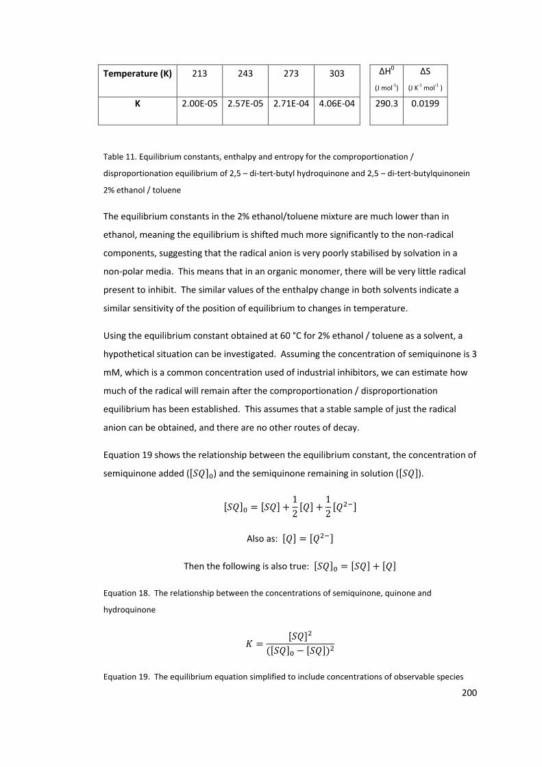
200
Temperature (K) 213 243 273 303 ∆H0
(J mol-1)
∆S
(J K-1 mol-1 )
K 2.00E-05 2.57E-05 2.71E-04 4.06E-04 290.3 0.0199
Table 11. Equilibrium constants, enthalpy and entropy for the comproportionation /
disproportionation equilibrium of 2,5 – di-tert-butyl hydroquinone and 2,5 – di-tert-butylquinonein
2% ethanol / toluene
The equilibrium constants in the 2% ethanol/toluene mixture are much lower than in
ethanol, meaning the equilibrium is shifted much more significantly to the non-radical
components, suggesting that the radical anion is very poorly stabilised by solvation in a
non-polar media. This means that in an organic monomer, there will be very little radical
present to inhibit. The similar values of the enthalpy change in both solvents indicate a
similar sensitivity of the position of equilibrium to changes in temperature.
Using the equilibrium constant obtained at 60 °C for 2% ethanol / toluene as a solvent, a
hypothetical situation can be investigated. Assuming the concentration of semiquinone is 3
mM, which is a common concentration used of industrial inhibitors, we can estimate how
much of the radical will remain after the comproportionation / disproportionation
equilibrium has been established. This assumes that a stable sample of just the radical
anion can be obtained, and there are no other routes of decay.
Equation 19 shows the relationship between the equilibrium constant, the concentration of
semiquinone added ([𝑆𝑄]0) and the semiquinone remaining in solution ([𝑆𝑄]).
[𝑆𝑄]0 = [𝑆𝑄] +1
2[𝑄] +
1
2[𝑄2−]
Also as: [𝑄] = [𝑄2−]
Then the following is also true: [𝑆𝑄]0 = [𝑆𝑄] + [𝑄]
Equation 18. The relationship between the concentrations of semiquinone, quinone and
hydroquinone
𝐾 =[𝑆𝑄]2
([𝑆𝑄]0 − [𝑆𝑄])2
Equation 19. The equilibrium equation simplified to include concentrations of observable species
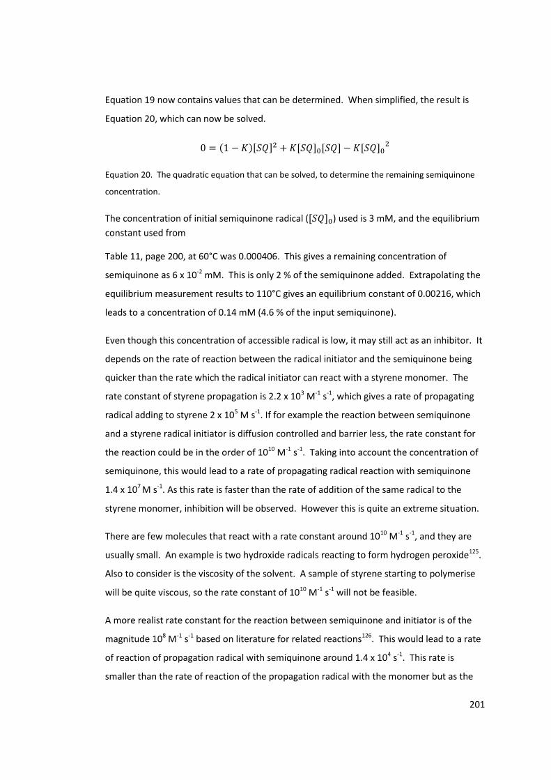
201
Equation 19 now contains values that can be determined. When simplified, the result is
Equation 20, which can now be solved.
0 = (1 − 𝐾)[𝑆𝑄]2 + 𝐾[𝑆𝑄]0[𝑆𝑄] − 𝐾[𝑆𝑄]02
Equation 20. The quadratic equation that can be solved, to determine the remaining semiquinone
concentration.
The concentration of initial semiquinone radical ([𝑆𝑄]0) used is 3 mM, and the equilibrium
constant used from
Table 11, page 200, at 60°C was 0.000406. This gives a remaining concentration of
semiquinone as 6 x 10⁻² mM. This is only 2 % of the semiquinone added. Extrapolating the
equilibrium measurement results to 110°C gives an equilibrium constant of 0.00216, which
leads to a concentration of 0.14 mM (4.6 % of the input semiquinone).
Even though this concentration of accessible radical is low, it may still act as an inhibitor. It
depends on the rate of reaction between the radical initiator and the semiquinone being
quicker than the rate which the radical initiator can react with a styrene monomer. The
rate constant of styrene propagation is 2.2 x 10³ M-1 s-1, which gives a rate of propagating
radical adding to styrene 2 x 10⁵ M s-1. If for example the reaction between semiquinone
and a styrene radical initiator is diffusion controlled and barrier less, the rate constant for
the reaction could be in the order of 1010 M-1 s-1. Taking into account the concentration of
semiquinone, this would lead to a rate of propagating radical reaction with semiquinone
1.4 x 10⁷ M s-1. As this rate is faster than the rate of addition of the same radical to the
styrene monomer, inhibition will be observed. However this is quite an extreme situation.
There are few molecules that react with a rate constant around 1010 M-1 s-1, and they are
usually small. An example is two hydroxide radicals reacting to form hydrogen peroxide125.
Also to consider is the viscosity of the solvent. A sample of styrene starting to polymerise
will be quite viscous, so the rate constant of 1010 M-1 s-1 will not be feasible.
A more realist rate constant for the reaction between semiquinone and initiator is of the
magnitude 108 M-1 s-1 based on literature for related reactions126. This would lead to a rate
of reaction of propagation radical with semiquinone around 1.4 x 10⁴ s-1. This rate is
smaller than the rate of reaction of the propagation radical with the monomer but as the
202
calculations include significant uncertainty, it is possible that some retardation of
polymerisation would be observed. Without knowing the exact rate of reaction between
semiquinone and initiator, it is only speculation, but it is doubtful the semiquinone would
be an effective inhibitor.
In reality, obtaining a stable quantity of semiquinone and dissolving it in organic media
without it decomposing via any other routes is not possible. However this exercise shows
that any semiquinone that does form in organic media, through a comproportionation /
disproportionation equilibrium or charge transfer catalyst, will be present at a fairly low
steady state concentration and hence is unlikely to act as a good inhibitor.
5.4 Conclusions
Chloranil radical anion was proposed as the inhibiting species in a chloranil / tertiary amine
charge transfer complex.61 The potassium salt of the radical anion was therefore
investigated as a potential inhibitor. However this salt is not soluble in organic media. This
limits its use as a potential inhibitor.
When the chloranil radical anion potassium salt is observed in water, it is unstable and the
EPR signal decays. By observing the decomposition products, it can be concluded that the
radical is susceptible to nucleophilic substitutions and oxidation, and reactions with
another radical. This suggests that the chloranil radical anion formed by the decomposition
of the charge transfer complex, is unlikely to survive and act as an inhibitor.
When using an inert atmosphere, the rate of decay decreases. This suggests the radical
anion is easily oxidised, but that there is still a route for decay, presumably through self-
reactions.
The comproportionation/disproportionation equilibrium in the quinone-hydroquinone
mixture was explored in order to estimate the steady state concentration of semiquinone
in solution, to understand if realistically the semiquinone formed by the degradation of a
charge transfer complex can act as an inhibitor. This could not be done with chloranil and
tetrachloro hydroquinone due to the high reactivity of the starting materials. The use of
203
2,5 – di-tert-butylquinone and the 2,5 – di-tert-butyl hydroquinone was possible and
investigated as an alternative.
In ethanol, the comproportionation/disproportionation equilibrium for the 2,5 – di-tert-
butylquinone and the 2,5 – di-tert-butyl hydroquinone is shifted to the non-radical
components, as determined from the equilibrium constant. At lower temperatures, the
equilibrium shifts even further to the non-radical components. In a more non-polar
medium (e.g., 2% ethanol / toluene mixture), the equilibrium concentration of
semiquinone is even lower.
By taking into account the equilibrium concentration of semiquinone under realistic
conditions, and comparing the hypothetical rates of reaction between the semiquinone
and styrene initiator radicals, we conclude that the semiquinone is unlikely to react fast
enough with the propagating radials to inhibit the polymerisation. It can be concluded
therefore that the inhibition observed by Yassin and Rizk61 is likely to be caused by the
trapping of the propagating radicals by the charge transfer complex itself rather than free
semiquinone radical anion formed by the degradation of the charge transfer complex.
204
6. Final conclusions
The overall mission of this study was to develop a better understanding of the mode of
action of inhibitors of spontaneous polymerisation. The initial part of the study was to first
determine how the current inhibition methods work on a mechanistic level. It has been
determined that the current industry standard inhibitor, DNBP, inhibits through aromatic
nitro groups. It is more efficacious than nitrobenzene due to the interaction between the
ortho nitro and phenol groups. The hydrogen bonding between them makes the nitro
group more susceptible to attack by the radicals formed through spontaneous initiation.
The product analysis of styrene inhibited by 2-nitrophenol, a similar molecule to DNBP, has
determined a number of products. The mechanism of formation of the intermediate
Unknown B was studied, by purposely synthesising it. Through this it has been
hypothesised that an imine intermediate is formed, supporting that nitrophenol inhibitors
work though the nitro group.
The side products from this initial reaction were investigated. They do not inhibit
polymerisation effectively. Also, by comparing the rate of formation of initiator radicals in
spontaneous polymerisation, and the rate of nitrophenol inhibitor consumption, it can be
suggested that the inhibition reaction is stoichiometric. This shows that there is no
catalytic cycle set up, which would have made nitrophenol inhibitors more effective.
A possible new inhibitor has been investigated. The proposed mechanism of action is the
charge transfer complex between chloranil and N,N-dimethyl aniline. The proposed
inhibiting species, the chloranil radical anion has been found to be too unstable to be the
molecule responsible for inhibition. Investigating 2,5-ditertbutyl quinone as a substitute
for chloranil showed that a semiquinone intermediate is unlikely to inhibit.
Using the comproportionation / disproportionation equilibrium as a measure of its stability,
showed that the equilibrium strongly favours the non-radical products. Therefore it is
unlikely that the semiquinone radical would be available in high enough concentration to
inhibit the spontaneously initiated polymerisation.
As the presence of a nitro group is essential for DNBP to work, and nitro compounds are
too toxic by according to new legislation, it may not be possible to develop new inhibitors

205
based on such compounds; hence alternative mechanisms should be targeted. The quinone
example shows that there is a lot of promise in synergistic action of mixtures of different
inhibitors, even though the mechanisms are quite hard to understand in these cases; you
can predict therefore that this is where the future research may be concentrated
206
7. Experimental
7.1 Chemicals and materials
All chemicals including deuterated solvents were purchased from Sigma-Aldrich, and used,
unless stated, without further purification. Solvents were supplied by Fisher, and were
used without further purification, unless otherwise stated. DNBP was provided by Nufarm
UK Ltd.
7.1.1 Styrene preparation
Stock styrene from Aldrich included a transport inhibitor, 4-tert-butylcatechol, at ~10ppm.
Inhibitor was removed by running styrene through alumina column immediately before
use.
7.2 NMR
1H and 13C NMR spectra were recorded in the deuterated solvent as indicated, on JEOL ECX
270 MHz, ECX 400 MHz or ECS 400 MHz spectrometers. Chemical shifts are reported in
parts per million using the deuterated solvent as a internal reference. Spin multiplicities are
indicated by the following symbols: s (singlet), d (doublet), t (triplet), q (quartet), qu
(quintet), sx (sextet), sept (septet), m (multiplet), br (broad).
207
7.3 EPR
Electron paramagnetic resonance spectra were recorded on a JEOL JES-RE1X X-band
spectrometer. A sealed Pasteur pipette was used for samples unless otherwise stated.
Typical parameters were; power 5.0 mW, frequency 9.105 GHz, field modulation width 1.0
G, sweep time 90 s.
Where spectra were averaged, scans were recorded individually at a set time interval and
manipulated using Spectrum Viewer Plus 2.6.3.
7.4 MS
Mass spectra, both positive and negative mode, were recorded on a Bruker micro-TOF with
LCQ ion trap with electron spray ionisation. The samples were dissolved in an appropriate
solvent and then diluted in methanol or acetonitrile as needed. The approximate
concentration of a sample is 5 mg of sample in 2 ml of solvent, dependent on solubility of
the sample, and how much of the sample was available. The solution was then submitted
to the mass spectrometer by an Agilent 1200 series Liquid Chromatography system pump.
No chromatography was performed by the equipment.
7.5 Dilatometry
Samples were prepared at 0.1M concentration (5 mL scale unless limited inhibitor
available). Fine glass pipette was used to insert sample into capillary tube. Compressed air
and fine pipette were used to remove excess styrene and inhibitor from headspace.
Samples were sealed by Bunsen burner.
Oil bath was pre-heated to 113°C for a 110°C experiment. Temperature was reset to 110°C
once rack was inserted into bath. Images of rack were taken immediately after insertion.
208
7.6 Oximetry (Oxygen diffusion into chlorobenzene)
TEMPO (100ppm) solution in chlorobenzene (5 mL) was prepared in a sample vial open to
air. This solution (0.1mL) was added to a sealed Pasteur pipette and oxygen was removed
by freeze-pump-thaw method under nitrogen. In the final stage, the headspace was
evacuated with the sample frozen, and backfilled with air while keeping the sample frozen.
This ensured the absence of oxygen in the solution which is exposed to air. The sample was
carefully moved from Schlenk line to EPR machine, and thawed, keeping the sample
undisturbed when inserting into EPR spectrometer.
7.7 Column Chromatography / Thin Layer
Chromatography
Flash column chromatography was performed with Fluka Analytical Silica Gel 60 (pores size
60 Å, 220-440 mesh particle size, 35-75 μm particle size). TLC was performed using Merck
TLC Silica 60 F256 on aluminium sheets, cut into smaller tiles before use.
7.8 X-ray crystallography
A sample of Unknown B was dissolved in CDCl3 and the solvent allowed to evaporate at
room temperature in an open vial to produce crystals. A suitable crystal was selected and
the experiment was performed on an Oxford Diffraction Supernova diffractometer. The
crystal was kept at 109.9(2) K during data collection. Using Olex2127, the structure was
solved with the Superflip128 structure solution program using Charge Flipping and refined
with the ShelXL129 refinement package using Least Squares minimisation.
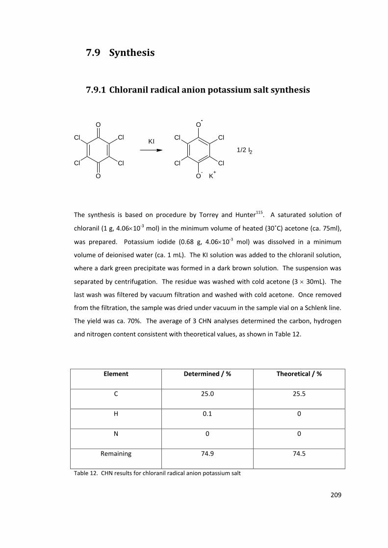
209
7.9 Synthesis
7.9.1 Chloranil radical anion potassium salt synthesis
Cl Cl
ClCl
O
O
Cl Cl
ClCl
O-
O
KI
K+
1/2 I2
The synthesis is based on procedure by Torrey and Hunter115. A saturated solution of
chloranil (1 g, 4.0610-3 mol) in the minimum volume of heated (30˚C) acetone (ca. 75ml),
was prepared. Potassium iodide (0.68 g, 4.0610-3 mol) was dissolved in a minimum
volume of deionised water (ca. 1 mL). The KI solution was added to the chloranil solution,
where a dark green precipitate was formed in a dark brown solution. The suspension was
separated by centrifugation. The residue was washed with cold acetone (3 30mL). The
last wash was filtered by vacuum filtration and washed with cold acetone. Once removed
from the filtration, the sample was dried under vacuum in the sample vial on a Schlenk line.
The yield was ca. 70%. The average of 3 CHN analyses determined the carbon, hydrogen
and nitrogen content consistent with theoretical values, as shown in Table 12.
Element Determined / % Theoretical / %
C 25.0 25.5
H 0.1 0
N 0 0
Remaining 74.9 74.5
Table 12. CHN results for chloranil radical anion potassium salt
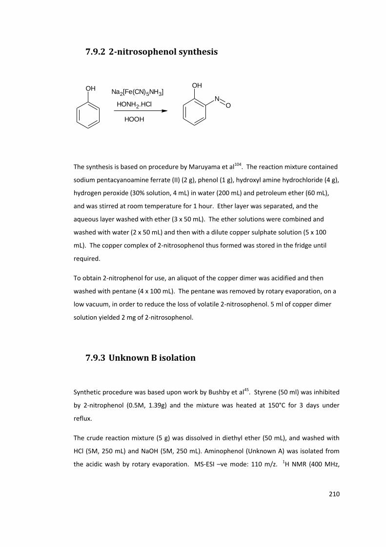
210
7.9.2 2-nitrosophenol synthesis
OHNa2[Fe(CN)5NH3]
HONH2.HCl
HOOH
OH
NO
The synthesis is based on procedure by Maruyama et al104. The reaction mixture contained
sodium pentacyanoamine ferrate (II) (2 g), phenol (1 g), hydroxyl amine hydrochloride (4 g),
hydrogen peroxide (30% solution, 4 mL) in water (200 mL) and petroleum ether (60 mL),
and was stirred at room temperature for 1 hour. Ether layer was separated, and the
aqueous layer washed with ether (3 x 50 mL). The ether solutions were combined and
washed with water (2 x 50 mL) and then with a dilute copper sulphate solution (5 x 100
mL). The copper complex of 2-nitrosophenol thus formed was stored in the fridge until
required.
To obtain 2-nitrophenol for use, an aliquot of the copper dimer was acidified and then
washed with pentane (4 x 100 mL). The pentane was removed by rotary evaporation, on a
low vacuum, in order to reduce the loss of volatile 2-nitrosophenol. 5 ml of copper dimer
solution yielded 2 mg of 2-nitrosophenol.
7.9.3 Unknown B isolation
Synthetic procedure was based upon work by Bushby et al45. Styrene (50 ml) was inhibited
by 2-nitrophenol (0.5M, 1.39g) and the mixture was heated at 150°C for 3 days under
reflux.
The crude reaction mixture (5 g) was dissolved in diethyl ether (50 mL), and washed with
HCl (5M, 250 mL) and NaOH (5M, 250 mL). Aminophenol (Unknown A) was isolated from
the acidic wash by rotary evaporation. MS-ESI –ve mode: 110 m/z. 1H NMR (400 MHz,
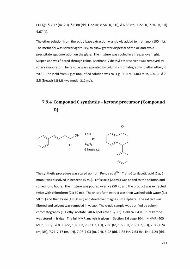
211
CDCl3): δ 7.17 (m, 2H), δ 6.88 (dd, 1.22 Hz, 8.54 Hz, 1H), δ 6.83 (td, 1.22 Hz, 7.94 Hz, 1H)
4.67 (s).
The ether solution from the acid / base extraction was slowly added to methanol (100 mL).
The methanol was stirred vigorously, to allow greater dispersal of the oil and avoid
precipitate agglomeration on the glass. The mixture was cooled in a freezer overnight.
Suspension was filtered through celite. Methanol / diethyl ether solvent was removed by
rotary evaporator. The residue was separated by column chromatography (diethyl ether, Rf
~0.5). The yield from 5 g of unpurified solution was ca. 1 g. 1H NMR (400 MHz, CDCl3): δ 7-
8.5 (Broad) ESI-MS –ve mode: 312 m/z.
7.9.4 Compound C synthesis – ketone precursor (Compound
D)
OH
O
O
TfOH
C6H6
6 hours r.t.
The synthetic procedure was scaled up from Rendy et al100. Trans-Styrylacetic acid (1 g, 6
mmol) was dissolved in benzene (5 mL). Triflic acid (20 mL) was added to the solution and
stirred for 6 hours. The mixture was poured over ice (50 g), and the product was extracted
twice with chloroform (2 x 50 ml). The chloroform extract was then washed with water (3 x
50 mL) and then brine (1 x 50 mL) and dried over magnesium sulphate. The extract was
filtered and solvent was removed in vacuo. The crude sample was purified by column
chromatography (1:1 ethyl acetate : 40-60 pet ether, Rf 0.3) Yield ca. 64 %. Pure ketone
was stored in fridge. The full NMR analysis is given in Section 3.6 page 104. 1H NMR (400
MHz, CDCl3): δ 8.06 (dd, 1.83 Hz, 7.93 Hz, 1H), 7.36 (td, 1.53 Hz, 7.63 Hz, 3H), 7.30-7.24
(m, 3H), 7.21-7.17 (m, 1H), 7.06-7.03 (m, 2H), 6.92 (dd, 1.83 Hz, 7.63 Hz, 1H), 4.24 (dd,
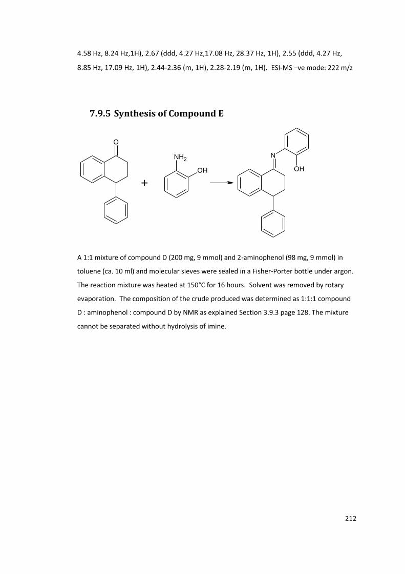
212
4.58 Hz, 8.24 Hz,1H), 2.67 (ddd, 4.27 Hz,17.08 Hz, 28.37 Hz, 1H), 2.55 (ddd, 4.27 Hz,
8.85 Hz, 17.09 Hz, 1H), 2.44-2.36 (m, 1H), 2.28-2.19 (m, 1H). ESI-MS –ve mode: 222 m/z
7.9.5 Synthesis of Compound E
O
+
NH2
OH
N
OH
A 1:1 mixture of compound D (200 mg, 9 mmol) and 2-aminophenol (98 mg, 9 mmol) in
toluene (ca. 10 ml) and molecular sieves were sealed in a Fisher-Porter bottle under argon.
The reaction mixture was heated at 150°C for 16 hours. Solvent was removed by rotary
evaporation. The composition of the crude produced was determined as 1:1:1 compound
D : aminophenol : compound D by NMR as explained Section 3.9.3 page 128. The mixture
cannot be separated without hydrolysis of imine.

213
7.9.6 Compound E to Compound C reaction
N
OH
N
O
A 0.1 M Compound D / E / 2-aminophenol mixture (from above) in 1:1 styrene : toluene (1
mL) was heated for 4 hours. The product mixture was analysed as described in Section
3.9.4 page 130. ESI-MS: Loss of 314 m/z during reaction. Occurrence of 312 m/z as
reaction progressed.
7.9.7 N-(1-Phenylethylene)-o-aminophenol – Compound F
CH3
O
NH2
OH
CH3
N
OH
The synthesis followed the procedure by Tauer and Grellmann102. 2-Aminophenol (0.2 mol)
and acetophenone (0.22 mol) were refluxed in toluene (150 mL) in a Dean-Stark apparatus,
until 0.2 mol of water were removed. The reaction mixture was concentrated by 50% and
solid was separated by vacuum filtration. The yield was 55 %. MS-ESI –ve mode: 210.1
m/z. 1H NMR (400 MHz, CDCl3): δ 8.02 (dd, 1.53 Hz, 8.09 Hz, 2H), δ 7.48 (m, 3H), δ 7.09

214
(td, 1.53 Hz, 7.32 Hz, 1H), δ 7.00 (dd, 1.22 Hz, 8.09 Hz, 1H), δ 6.89 (td, 1.53 Hz, 7.32 Hz
1H), δ 6.80 (dd, 1.53 Hz, 7.63 Hz, 1H), δ 2.45 (s, 3H)

215
8. Appendices
The following are the spectra and tables of information referred to in the previous text
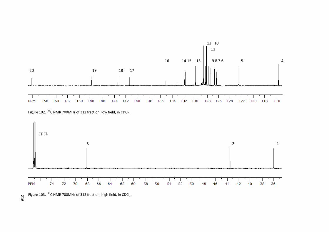
216
Figure 102. 13
C NMR 700MHz of 312 fraction, low field, in CDCl3.
Figure 103. 13
C NMR 700MHz of 312 fraction, high field, in CDCl3.
16 14 15 13 9 8 7 6 5 4
18 17 19 20
CDCl3
3 2 1
12 10
11
21
6
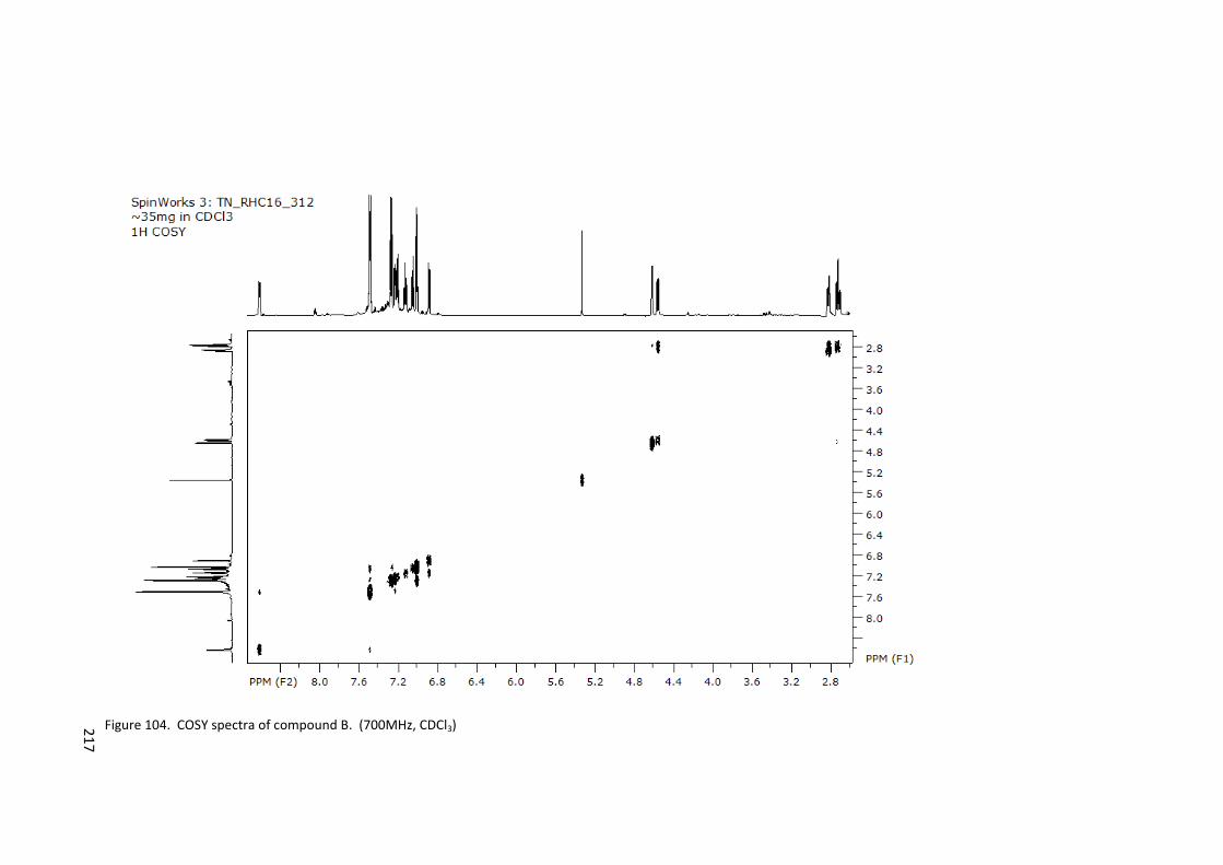
217
Figure 104. COSY spectra of compound B. (700MHz, CDCl3) 217
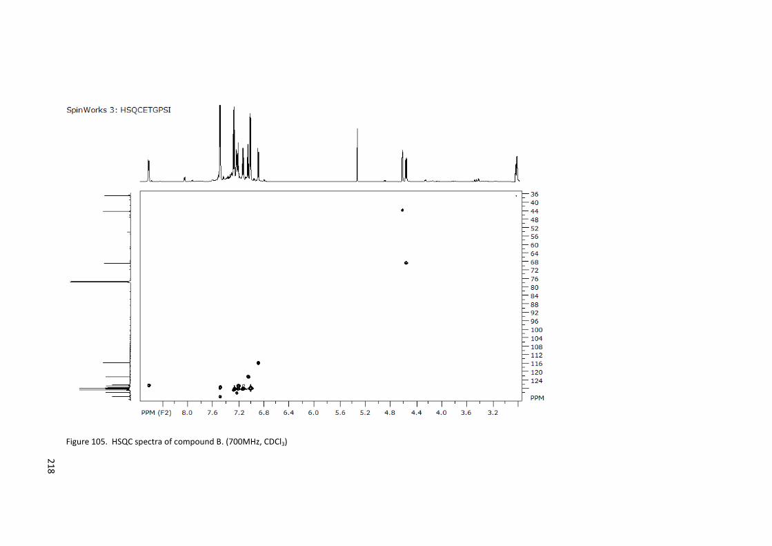
218
Figure 105. HSQC spectra of compound B. (700MHz, CDCl3)
218
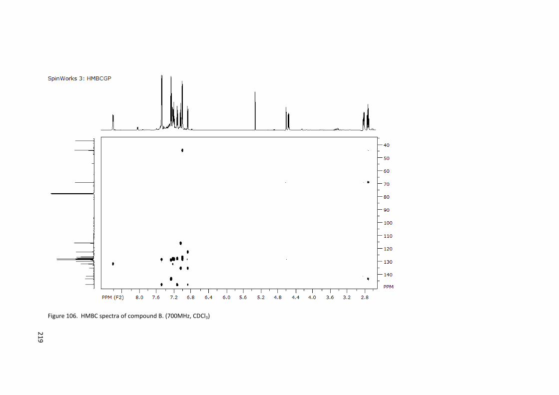
219
Figure 106. HMBC spectra of compound B. (700MHz, CDCl3)
219
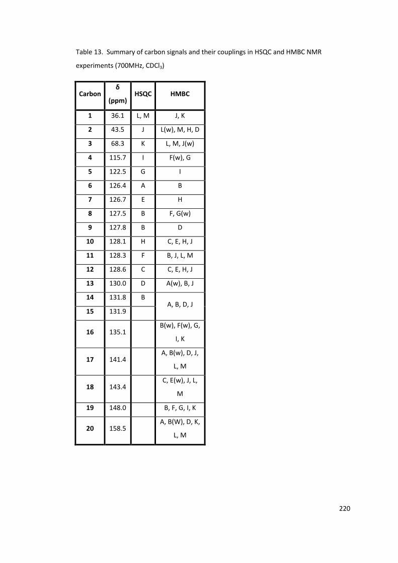
220
Table 13. Summary of carbon signals and their couplings in HSQC and HMBC NMR
experiments (700MHz, CDCl3)
Carbon δ
(ppm) HSQC HMBC
1 36.1 L, M J, K
2 43.5 J L(w), M, H, D
3 68.3 K L, M, J(w)
4 115.7 I F(w), G
5 122.5 G I
6 126.4 A B
7 126.7 E H
8 127.5 B F, G(w)
9 127.8 B D
10 128.1 H C, E, H, J
11 128.3 F B, J, L, M
12 128.6 C C, E, H, J
13 130.0 D A(w), B, J
14 131.8 B A, B, D, J
15 131.9
16 135.1 B(w), F(w), G,
I, K
17 141.4 A, B(w), D, J,
L, M
18 143.4 C, E(w), J, L,
M
19 148.0 B, F, G, I, K
20 158.5 A, B(W), D, K,
L, M
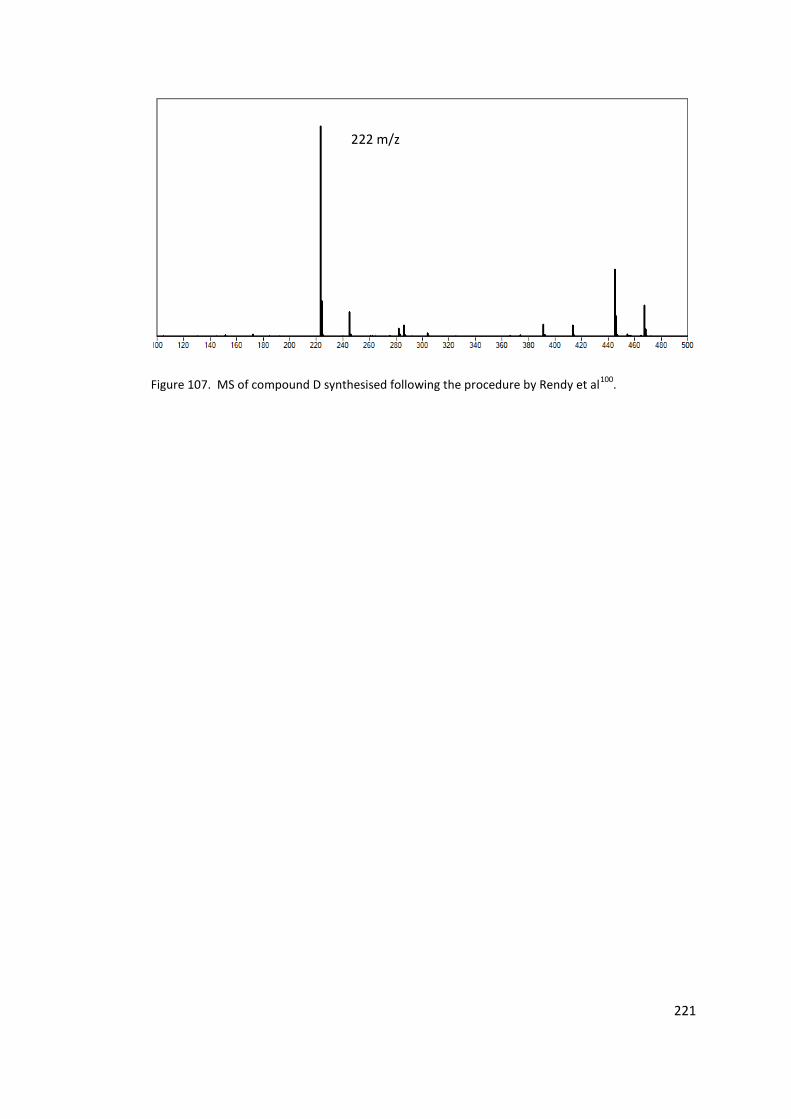
221
Figure 107. MS of compound D synthesised following the procedure by Rendy et al100
.
222 m/z
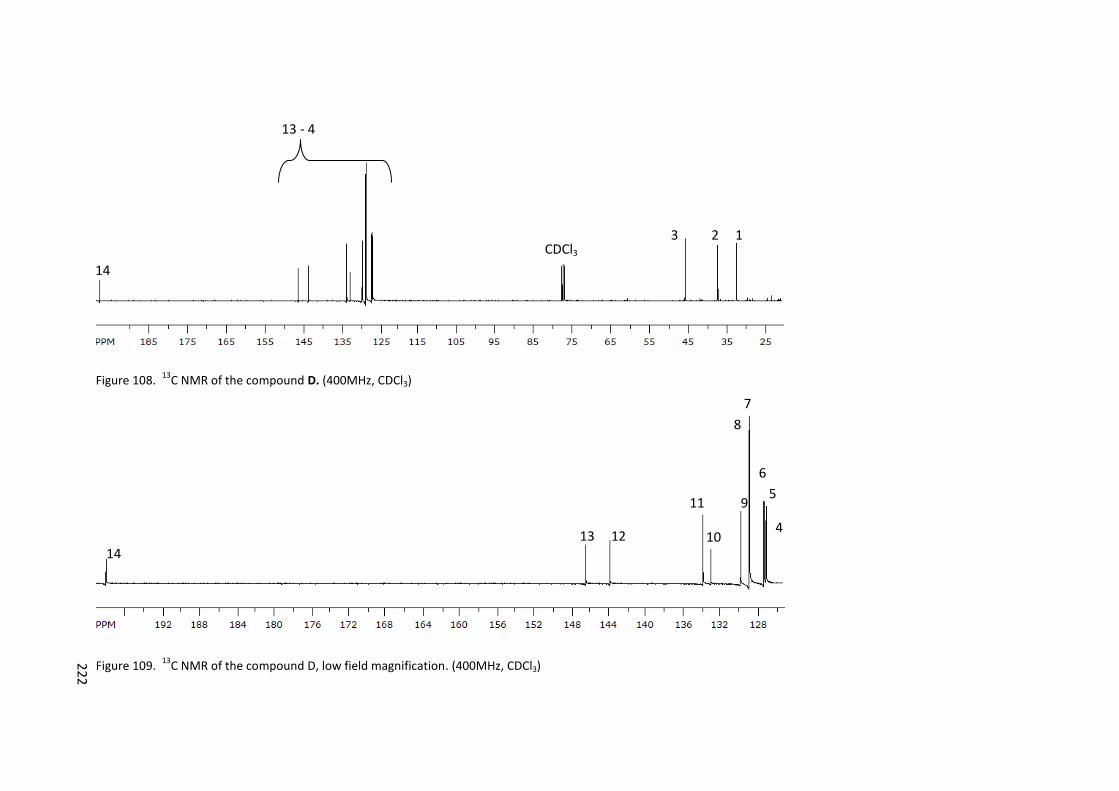
222
Figure 108. 13
C NMR of the compound D. (400MHz, CDCl3)
Figure 109. 13
C NMR of the compound D, low field magnification. (400MHz, CDCl3)
13 - 4
14
14
CDCl3 3 2 1
7
8
11 9
10 13 12
6
5
4
22
2
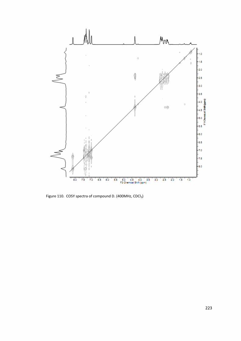
223
Figure 110. COSY spectra of compound D. (400MHz, CDCl3)
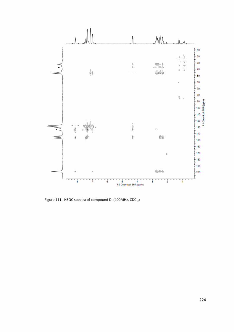
224
Figure 111. HSQC spectra of compound D. (400MHz, CDCl3)
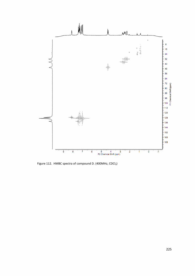
225
Figure 112. HMBC spectra of compound D. (400MHz, CDCl3)
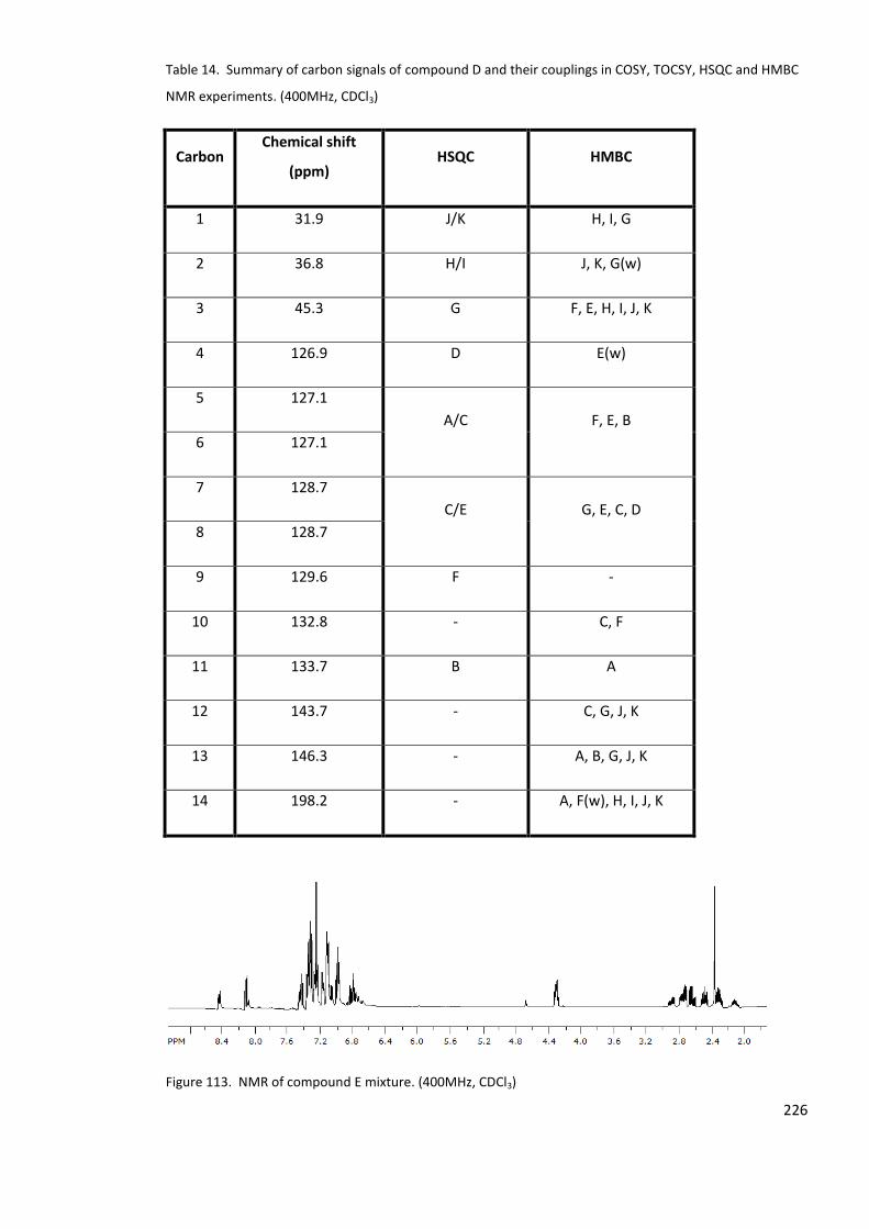
226
Table 14. Summary of carbon signals of compound D and their couplings in COSY, TOCSY, HSQC and HMBC
NMR experiments. (400MHz, CDCl3)
Carbon Chemical shift
(ppm) HSQC HMBC
1 31.9 J/K H, I, G
2 36.8 H/I J, K, G(w)
3 45.3 G F, E, H, I, J, K
4 126.9 D E(w)
5 127.1
A/C F, E, B
6 127.1
7 128.7
C/E G, E, C, D
8 128.7
9 129.6 F -
10 132.8 - C, F
11 133.7 B A
12 143.7 - C, G, J, K
13 146.3 - A, B, G, J, K
14 198.2 - A, F(w), H, I, J, K
Figure 113. NMR of compound E mixture. (400MHz, CDCl3)
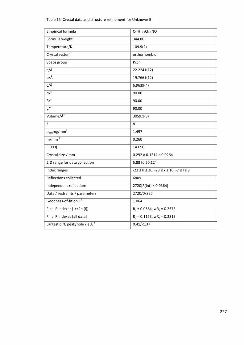
227
Table 15. Crystal data and structure refinement for Unknown B
Empirical formula C22H14.5Cl0.5NO
Formula weight 344.80
Temperature/K 109.9(2)
Crystal system orthorhombic
Space group Pccn
a/Å 22.2241(12)
b/Å 19.7661(12)
c/Å 6.9639(4)
α/° 90.00
β/° 90.00
γ/° 90.00
Volume/Å3 3059.1(3)
Z 8
ρcalcmg/mm3 1.497
m/mm-1
0.260
F(000) 1432.0
Crystal size / mm
0.292 × 0.1214 × 0.0264
2 Θ range for data collection 5.88 to 50.12°
Index ranges -22 ≤ h ≤ 26, -23 ≤ k ≤ 10, -7 ≤ l ≤ 8
Reflections collected 6809
Independent reflections 2720[R(int) = 0.0364]
Data / restraints / parameters 2720/0/226
Goodness-of-fit on F2 1.064
Final R indexes [I>=2σ (I)] R1 = 0.0884, wR2 = 0.2573
Final R indexes [all data] R1 = 0.1153, wR2 = 0.2813
Largest diff. peak/hole / e Å-3
0.41/-1.37
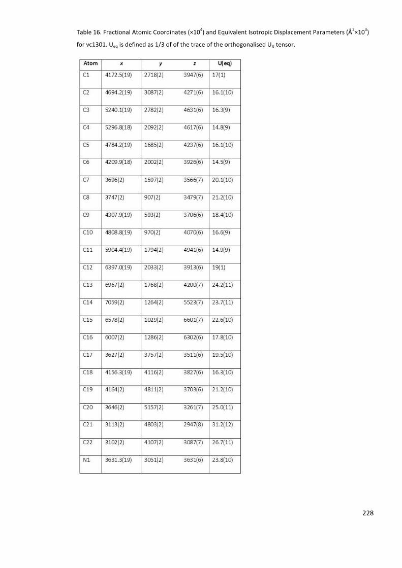
228
Table 16. Fractional Atomic Coordinates (×104) and Equivalent Isotropic Displacement Parameters (Å
2×10
3)
for vc1301. Ueq is defined as 1/3 of of the trace of the orthogonalised UIJ tensor.
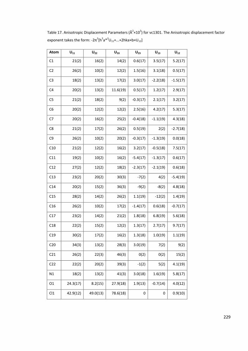
229
Table 17. Anisotropic Displacement Parameters (Å2×10
3) for vc1301. The Anisotropic displacement factor
exponent takes the form: -2π2[h
2a*
2U11+...+2hka×b×U12]
Atom U11 U22 U33 U23 U13 U12
C1 21(2) 16(2) 14(2) 0.6(17) 3.5(17) 5.2(17)
C2 26(2) 10(2) 12(2) 1.5(16) 3.1(18) 0.5(17)
C3 18(2) 13(2) 17(2) 3.0(17) -2.2(18) -1.5(17)
C4 20(2) 13(2) 11.6(19) 0.5(17) 1.2(17) 2.9(17)
C5 21(2) 18(2) 9(2) -0.3(17) 2.1(17) 3.2(17)
C6 20(2) 12(2) 12(2) 2.5(16) 4.2(17) 5.3(17)
C7 20(2) 16(2) 25(2) -0.4(18) -1.1(19) 4.3(18)
C8 21(2) 17(2) 26(2) 0.5(19) 2(2) -2.7(18)
C9 26(2) 10(2) 20(2) -0.3(17) -1.3(19) 0.0(18)
C10 21(2) 12(2) 16(2) 3.2(17) -0.5(18) 7.5(17)
C11 19(2) 10(2) 16(2) -5.4(17) -1.3(17) 0.6(17)
C12 27(2) 12(2) 18(2) -2.3(17) -2.1(19) 0.6(18)
C13 23(2) 20(2) 30(3) -7(2) 4(2) -5.4(19)
C14 20(2) 15(2) 36(3) -9(2) -8(2) 4.8(18)
C15 28(2) 14(2) 26(2) 1.1(19) -12(2) 1.4(19)
C16 26(2) 10(2) 17(2) -1.4(17) 0.6(18) -0.7(17)
C17 23(2) 14(2) 21(2) 1.8(18) 6.8(19) 5.6(18)
C18 22(2) 15(2) 12(2) 1.3(17) 2.7(17) 9.7(17)
C19 30(2) 17(2) 16(2) 1.3(18) 1.0(19) 1.1(19)
C20 34(3) 13(2) 28(3) 3.0(19) 7(2) 9(2)
C21 26(2) 22(3) 46(3) 0(2) 0(2) 15(2)
C22 22(2) 20(2) 39(3) -1(2) 5(2) 4.1(19)
N1 18(2) 13(2) 41(3) 3.0(18) 1.6(19) 5.8(17)
O1 24.3(17) 8.2(15) 27.9(18) 1.9(13) -0.7(14) 4.0(12)
Cl1 42.9(12) 49.0(13) 78.6(18) 0 0 0.9(10)
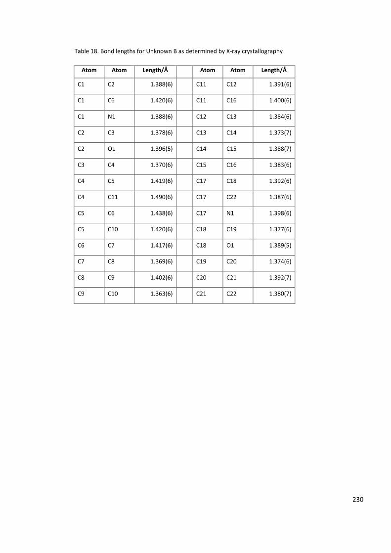
230
Table 18. Bond lengths for Unknown B as determined by X-ray crystallography
Atom Atom Length/Å Atom Atom Length/Å
C1 C2 1.388(6) C11 C12 1.391(6)
C1 C6 1.420(6) C11 C16 1.400(6)
C1 N1 1.388(6) C12 C13 1.384(6)
C2 C3 1.378(6) C13 C14 1.373(7)
C2 O1 1.396(5) C14 C15 1.388(7)
C3 C4 1.370(6) C15 C16 1.383(6)
C4 C5 1.419(6) C17 C18 1.392(6)
C4 C11 1.490(6) C17 C22 1.387(6)
C5 C6 1.438(6) C17 N1 1.398(6)
C5 C10 1.420(6) C18 C19 1.377(6)
C6 C7 1.417(6) C18 O1 1.389(5)
C7 C8 1.369(6) C19 C20 1.374(6)
C8 C9 1.402(6) C20 C21 1.392(7)
C9 C10 1.363(6) C21 C22 1.380(7)
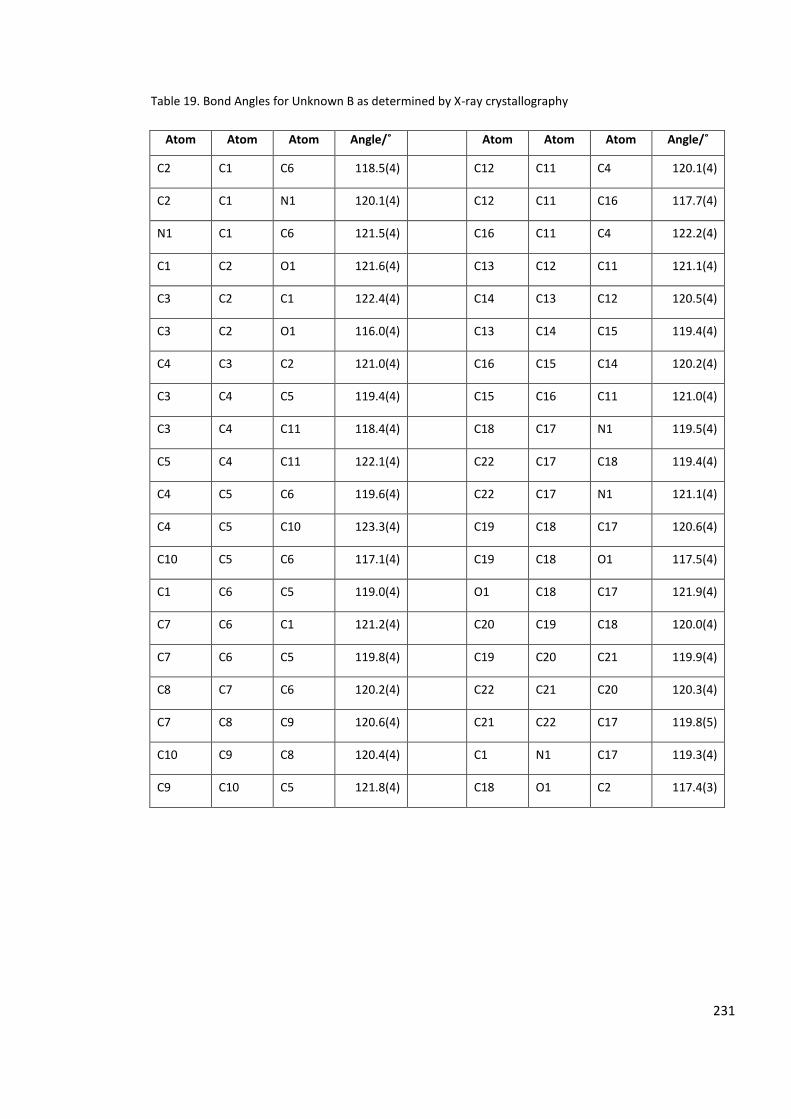
231
Table 19. Bond Angles for Unknown B as determined by X-ray crystallography
Atom Atom Atom Angle/˚ Atom Atom Atom Angle/˚
C2 C1 C6 118.5(4) C12 C11 C4 120.1(4)
C2 C1 N1 120.1(4) C12 C11 C16 117.7(4)
N1 C1 C6 121.5(4) C16 C11 C4 122.2(4)
C1 C2 O1 121.6(4) C13 C12 C11 121.1(4)
C3 C2 C1 122.4(4) C14 C13 C12 120.5(4)
C3 C2 O1 116.0(4) C13 C14 C15 119.4(4)
C4 C3 C2 121.0(4) C16 C15 C14 120.2(4)
C3 C4 C5 119.4(4) C15 C16 C11 121.0(4)
C3 C4 C11 118.4(4) C18 C17 N1 119.5(4)
C5 C4 C11 122.1(4) C22 C17 C18 119.4(4)
C4 C5 C6 119.6(4) C22 C17 N1 121.1(4)
C4 C5 C10 123.3(4) C19 C18 C17 120.6(4)
C10 C5 C6 117.1(4) C19 C18 O1 117.5(4)
C1 C6 C5 119.0(4) O1 C18 C17 121.9(4)
C7 C6 C1 121.2(4) C20 C19 C18 120.0(4)
C7 C6 C5 119.8(4) C19 C20 C21 119.9(4)
C8 C7 C6 120.2(4) C22 C21 C20 120.3(4)
C7 C8 C9 120.6(4) C21 C22 C17 119.8(5)
C10 C9 C8 120.4(4) C1 N1 C17 119.3(4)
C9 C10 C5 121.8(4) C18 O1 C2 117.4(3)
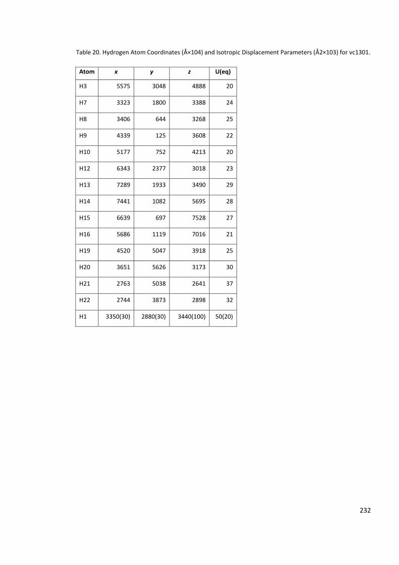
232
Table 20. Hydrogen Atom Coordinates (Å×104) and Isotropic Displacement Parameters (Å2×10³) for vc1301.
Atom x y z U(eq)
H3 5575 3048 4888 20
H7 3323 1800 3388 24
H8 3406 644 3268 25
H9 4339 125 3608 22
H10 5177 752 4213 20
H12 6343 2377 3018 23
H13 7289 1933 3490 29
H14 7441 1082 5695 28
H15 6639 697 7528 27
H16 5686 1119 7016 21
H19 4520 5047 3918 25
H20 3651 5626 3173 30
H21 2763 5038 2641 37
H22 2744 3873 2898 32
H1 3350(30) 2880(30) 3440(100) 50(20)
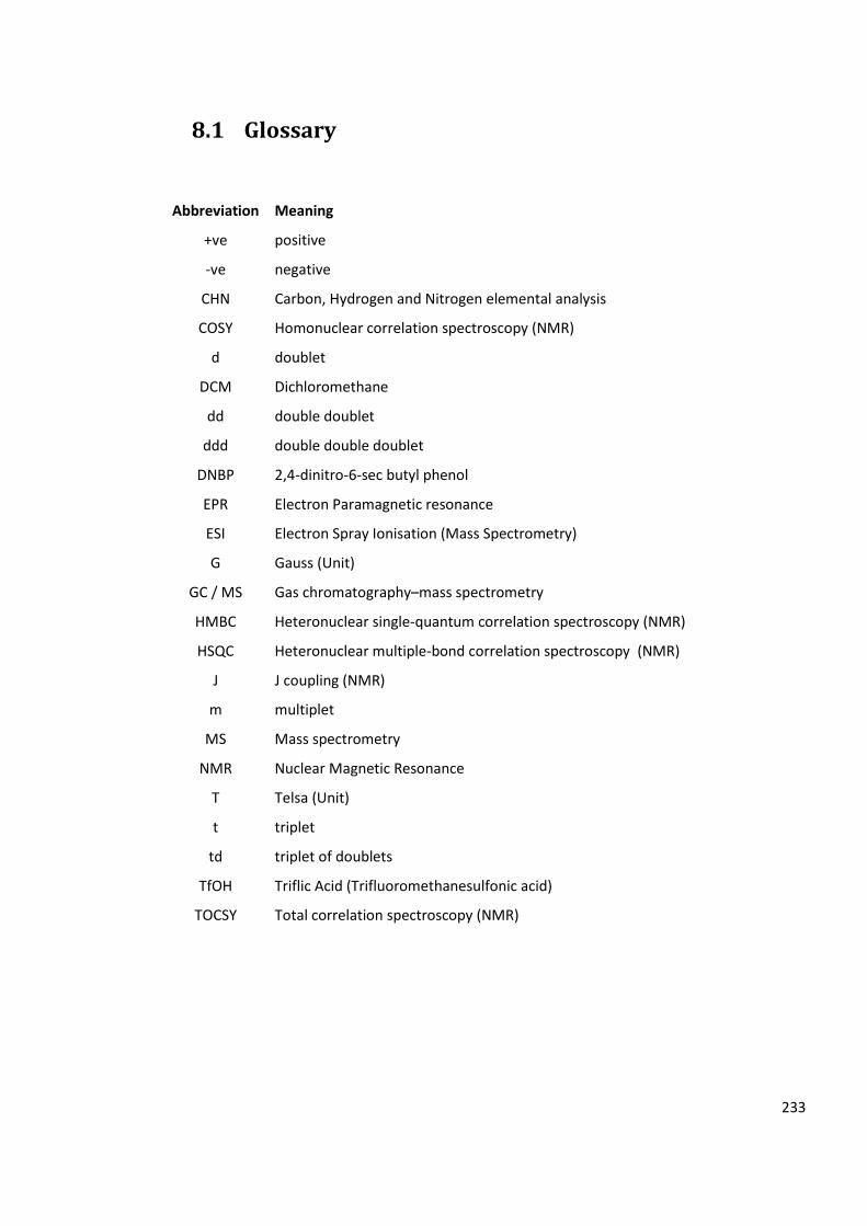
233
8.1 Glossary
Abbreviation Meaning
+ve positive
-ve negative
CHN Carbon, Hydrogen and Nitrogen elemental analysis
COSY Homonuclear correlation spectroscopy (NMR)
d doublet
DCM Dichloromethane
dd double doublet
ddd double double doublet
DNBP 2,4-dinitro-6-sec butyl phenol
EPR Electron Paramagnetic resonance
ESI Electron Spray Ionisation (Mass Spectrometry)
G Gauss (Unit)
GC / MS Gas chromatography–mass spectrometry
HMBC Heteronuclear single-quantum correlation spectroscopy (NMR)
HSQC Heteronuclear multiple-bond correlation spectroscopy (NMR)
J J coupling (NMR)
m multiplet
MS Mass spectrometry
NMR Nuclear Magnetic Resonance
T Telsa (Unit)
t triplet
td triplet of doublets
TfOH Triflic Acid (Trifluoromethanesulfonic acid)
TOCSY Total correlation spectroscopy (NMR)
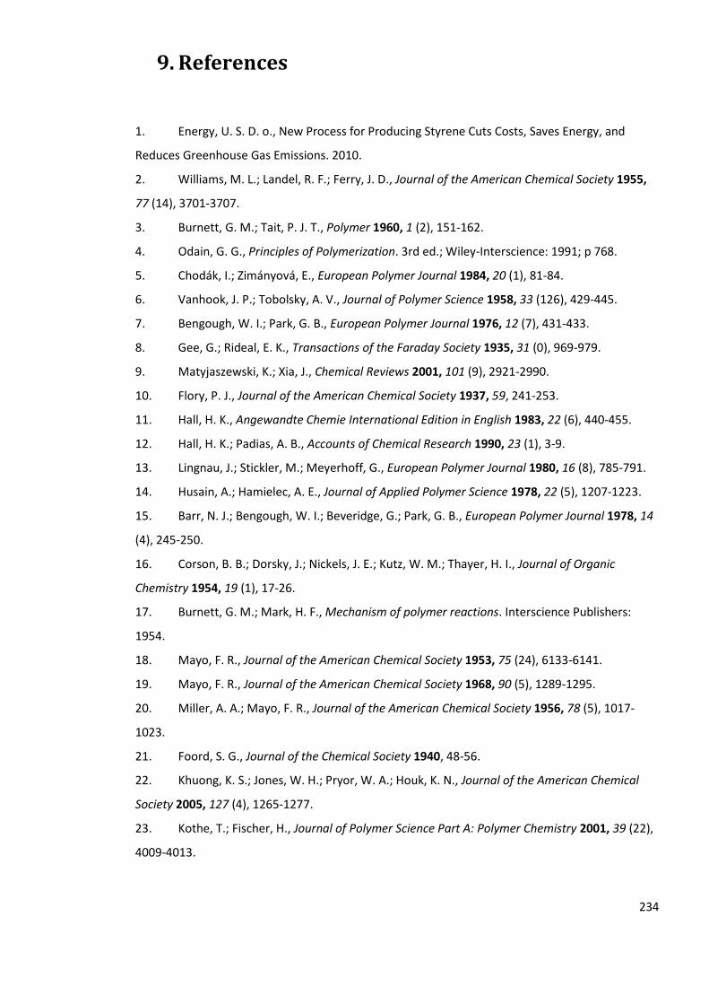
234
9. References
1. Energy, U. S. D. o., New Process for Producing Styrene Cuts Costs, Saves Energy, and
Reduces Greenhouse Gas Emissions. 2010.
2. Williams, M. L.; Landel, R. F.; Ferry, J. D., Journal of the American Chemical Society 1955,
77 (14), 3701-3707.
3. Burnett, G. M.; Tait, P. J. T., Polymer 1960, 1 (2), 151-162.
4. Odain, G. G., Principles of Polymerization. 3rd ed.; Wiley-Interscience: 1991; p 768.
5. Chodák, I.; Zimányová, E., European Polymer Journal 1984, 20 (1), 81-84.
6. Vanhook, J. P.; Tobolsky, A. V., Journal of Polymer Science 1958, 33 (126), 429-445.
7. Bengough, W. I.; Park, G. B., European Polymer Journal 1976, 12 (7), 431-433.
8. Gee, G.; Rideal, E. K., Transactions of the Faraday Society 1935, 31 (0), 969-979.
9. Matyjaszewski, K.; Xia, J., Chemical Reviews 2001, 101 (9), 2921-2990.
10. Flory, P. J., Journal of the American Chemical Society 1937, 59, 241-253.
11. Hall, H. K., Angewandte Chemie International Edition in English 1983, 22 (6), 440-455.
12. Hall, H. K.; Padias, A. B., Accounts of Chemical Research 1990, 23 (1), 3-9.
13. Lingnau, J.; Stickler, M.; Meyerhoff, G., European Polymer Journal 1980, 16 (8), 785-791.
14. Husain, A.; Hamielec, A. E., Journal of Applied Polymer Science 1978, 22 (5), 1207-1223.
15. Barr, N. J.; Bengough, W. I.; Beveridge, G.; Park, G. B., European Polymer Journal 1978, 14
(4), 245-250.
16. Corson, B. B.; Dorsky, J.; Nickels, J. E.; Kutz, W. M.; Thayer, H. I., Journal of Organic
Chemistry 1954, 19 (1), 17-26.
17. Burnett, G. M.; Mark, H. F., Mechanism of polymer reactions. Interscience Publishers:
1954.
18. Mayo, F. R., Journal of the American Chemical Society 1953, 75 (24), 6133-6141.
19. Mayo, F. R., Journal of the American Chemical Society 1968, 90 (5), 1289-1295.
20. Miller, A. A.; Mayo, F. R., Journal of the American Chemical Society 1956, 78 (5), 1017-
1023.
21. Foord, S. G., Journal of the Chemical Society 1940, 48-56.
22. Khuong, K. S.; Jones, W. H.; Pryor, W. A.; Houk, K. N., Journal of the American Chemical
Society 2005, 127 (4), 1265-1277.
23. Kothe, T.; Fischer, H., Journal of Polymer Science Part A: Polymer Chemistry 2001, 39 (22),
4009-4013.
235
24. Zhang, C.; Wang, X.; Liu, L.; Wang, Y.; Peng, X., Journal of Molecular Modeling 2008, 14
(11), 1053-1064.
25. Stickler, M.; Meyerhoff, G., Makromolekulare Chemie-Macromolecular Chemistry and
Physics 1980, 181 (1), 131-147.
26. Stickler, M.; Meyerhoff, G., Polymer 1981, 22 (7), 928-933.
27. Lehrle, R. S.; Shortland, A., European Polymer Journal 1988, 24 (5), 425-429.
28. Lingnau, J.; Meyerhoff, G., Macromolecules 1984, 17 (4), 941-945.
29. Albisetti, C. J.; England, D. C.; Hogsed, M. J.; Joyce, R. M., Journal of the American
Chemical Society 1956, 78 (2), 472-475.
30. Bhanu, V. A.; Kishore, K., Chemical Reviews 1991, 91 (2), 99-117.
31. Graham, W. D.; Green, J. G.; Pryor, W. A., Journal of Organic Chemistry 1979, 44 (6), 907-
914.
32. Hilditch, T. P., Nature 1950, 166 (4222), 558-559.
33. Khan, N. A., Journal of Chemical Physics 1953, 21 (5), 952-952.
34. Khan, N. A., Journal of Chemical Physics 1954, 22 (12), 2090-2090.
35. Khan, N. A., Canadian Journal of Chemistry-Revue Canadienne De Chimie 1959, 37 (6),
1029-1034.
36. Tornero-Velez, R.; Waidyanatha, S.; Echeverria, D.; Rappaport, S. M., Journal of
Environmental Monitoring 2000, 2 (2), 111-117.
37. Schulze, S.; Vogel, H., Chemical Engineering & Technology 1998, 21 (10), 829-837.
38. Denisov, E. T.; Afanas'ev, I. B., Oxidation and Antioxidants in Organic Chemistry and
Biology. Taylor & Francis: 2005.
39. Bevington, J. C.; Hunt, B. J., Journal of Macromolecular Science-Pure and Applied
Chemistry 2005, A42 (2), 203-210.
40. Kolyakina, E. V.; Grishin, D. F., Russian Chemical Reviews 2009, 78 (6), 535-568.
41. Lalevée, J.; Gigmes, D.; Bertin, D.; Allonas, X.; Fouassier, J. P., Chemical Physics Letters
2007, 449 (1-3), 231-235.
42. Greszta, D.; Matyjaszewski, K., Macromolecules 1996, 29 (24), 7661-7670.
43. Odell, P. G.; Veregin, R. P. N.; Michalak, L. M.; Georges, M. K., Macromolecules 1997, 30
(8), 2232-2237.
44. Webster, O. W., Science 1991, 251 (4996), 887-893.
45. Bushby, R. J.; Lord, N.; McRobbie, I.; Pryce, A., Polymer 1998, 39 (22), 5567-5571.
46. Jackson, R. A.; Waters, W. A., Journal of the Chemical Society 1960, (Apr), 1653-1657.
47. Tudos, F.; Foldesberezsnich, T., Progress in Polymer Science 1989, 14 (6), 717-761.
48. Gingras, B. A.; Waters, W. A., Journal of the Chemical Society 1954, (JUN), 1920-1924.
236
49. Motyakin, M. V.; Wasserman, A. M.; Stott, P. E.; Zaikov, G. E., Journal of Applied Polymer
Science 2004, 91 (3), 1599-1603.
50. Cohen, S. G., Journal of the American Chemical Society 1947, 69 (5), 1057-1064.
51. Cohen, S. G., Journal of Polymer Science 1947, 2 (5), 511-521.
52. Bevington, J. C.; Ghanem, N. A.; Melville, H. W., Journal of the Chemical Society 1955,
2822-2830.
53. Bevington, J. C.; Ghanem, N. A.; Melville, H. W., Transactions of the Faraday Society 1955,
51 (7), 946-953.
54. Eastmond, G. C., Chain Transfer, Inhibition and Retardation. In Comprehensive Chemical
Kinetics, 1st ed.; Bamford, C. H.; Tipper, C. F. H., Eds. Elsevier Scientific Publishing Company: 1976;
Vol. 14A, pp 105-152.
55. Levy, L. B., Journal of Polymer Science Part a-Polymer Chemistry 1992, 30 (4), 569-576.
56. Brand, R. H.; Hartwig, A.; Opitz, B.; Pfeifer, C.; Drochner, A.; Vogel, G. H., Macromolecular
Reaction Engineering 2011, 5 (5-6), 212-222.
57. Kolyakina, E. V.; Grishin, D. F., Russian Chemical Reviews 2011, 80 (7), 683-704.
58. Bickel, A. F.; Kooyman, E. C., Journal of the Chemical Society (Resumed) 1956, (0), 2215-
2221.
59. Atherton, N. M., Principles of Electron Spin Resonance. Ellis Horwood: 1993.
60. Gerson, F.; Huber, W., Part Introduction. In Electron Spin Resonance Spectroscopy of
Organic Radicals, Wiley-VCH Verlag GmbH & Co. KGaA: 2004; pp 1-1.
61. Yassin, A. A.; Rizk, N. A., British Polymer Journal 1977, 9 (4), 322-325.
62. Yun, M., Anitoxidant activity in styrene, Unpublished work. 2008.
63. Noel, L. F. J.; Brouwer, E. C. P.; Vanherk, A. M.; German, A. L., Journal of Applied Polymer
Science 1995, 57 (3), 245-254.
64. Hoogenboom, R.; Fijten, M. W. M.; Abeln, C. H.; Schubert, U. S., Macromolecular Rapid
Communications 2004, 25 (1), 237-242.
65. Jallapuram, R.; Naydenova, I.; Byrne, H. J.; Martin, S.; Howard, R.; Toal, V., Appl. Opt.
2008, 47 (2), 206-212.
66. McGill, C. A.; Ferguson, R. H.; Donoghue, K.; Nordon, A.; Littlejohn, D., Analyst 2003, 128
(12), 1467-1470.
67. Jovanovic, R.; Dube, M. A., Polymer Reaction Engineering 2003, 11 (3), 233-257.
68. Udagawa, A.; Sakurai, F.; Takahashi, T., Journal of Applied Polymer Science 1991, 42 (7),
1861-1867.
69. Aldridge, P. K.; Kelly, J. J.; Callis, J. B.; Burns, D. H., Analytical Chemistry 1993, 65 (24),
3581-3585.
237
70. Gulari, E.; McKeigue, K.; Ng, K. Y. S., Macromolecules 1984, 17 (9), 1822-1825.
71. Starkweather, H. W.; Taylor, G. B., Journal of the American Chemical Society 1930, 52 (12),
4708-4714.
72. Goldfinger, G.; Lauterbach, K. E., Journal of Polymer Science 1948, 3 (2), 145-156.
73. Schulz, G. V.; Harborth, G., Angewandte Chemie 1947, 59 (3), 90-92.
74. Patnode, W.; Scheiber, W. J., Journal of the American Chemical Society 1939, 61 (12),
3449-3451.
75. Nichols, F. S.; Flowers, R. G., Industrial & Engineering Chemistry 1950, 42 (2), 292-295.
76. Bernatchez, P.; Goutier, D., Review of Scientific Instruments 1973, 44 (12), 1790-1791.
77. Frey, S.; Richert, R., Review of Scientific Instruments 2010, 81 (3), 034702.
78. Karcz, J.; Strek, F., Chemical Engineering Journal and the Biochemical Engineering Journal
1995, 58 (2), 135-143.
79. Eckert, E. r. g.; Goldstein, R. J.; Ibele, W. e.; Patankar, S. V.; Simon, T. W.; Strykowski, P. J.;
Tamma, K. K.; Kuehn, T. H.; Bar-Cohen, A.; Heberlein, J. V. R.; Davidson, J. H.; Bischof, J.; Kulacki,
F.; Kortshagen, U., International Journal of Heat and Mass Transfer 1999, 42 (15), 2717-2797.
80. Conte, M.; Ma, Y.; Loyns, C.; Price, P.; Rippon, D.; Chechik, V., Organic & Biomolecular
Chemistry 2009, 7 (13), 2685-2687.
81. Smirnov, A. I.; Clarkson, R. B.; Belford, R. L., Journal of Magnetic Resonance, Series B 1996,
111 (2), 149-157.
82. Smirnova, T. I.; Smirnov, A. I., High-field ESR spectroscopy in membrane and protein
biophysics. In ESR Spectroscopy in Membrane Biophysics, Hemminga, M. A.; Berliner, L. J., Eds.
Kluwer Academic/Plenum Publ: New York, 2007; Vol. 27, pp 165-251.
83. Pedulli, G.; Lucarini, M.; Pedrielli, P.; Sagrini, M.; Cipollone, M., Research on Chemical
Intermediates 1996, 22 (1), 1-14.
84. East, G. C.; Margerison, D.; Pulat, E., Transactions of the Faraday Society 1966, 62 (0),
1301-1307.
85. Levy, L. B., Journal of Polymer Science: Polymer Chemistry Edition 1985, 23 (5), 1505-1515.
86. Kurland, J. J., Journal of Polymer Science: Polymer Chemistry Edition 1980, 18 (3), 1139-
1145.
87. Bakalbassis, E. G.; Lithoxoidou, A. T.; Vafiadis, A. P., The Journal of Physical Chemistry A
2006, 110 (38), 11151-11159.
88. Himo, F.; Eriksson, L. A.; Blomberg, M. R. A.; Siegbahn, P. E. M., International Journal of
Quantum Chemistry 2000, 76 (6), 714-723.
89. Hepworth, J. D.; Waring, D. R.; Waring, M. J.; Chemistry, R. S. o., Aromatic Chemistry.
Royal Society of Chemistry: 2002.
238
90. Lithoxoidou, A. T.; Bakalbassis, E. G., The Journal of Physical Chemistry A 2004, 109 (2),
366-377.
91. Korth, H.-G.; de Heer, M. I.; Mulder, P., The Journal of Physical Chemistry A 2002, 106 (37),
8779-8789.
92. Borges dos Santos, R. M.; Martinho Simões, J. A., J. Phys. Chem. Ref. Data 1998, 27 (3),
707-739.
93. Suryan, M. M.; Kafafi, S. A.; Stein, S. E., Journal of the American Chemical Society 1989,
111 (13), 4594-4600.
94. Bartlett, P. D.; Kwart, H., Journal of the American Chemical Society 1952, 74 (16), 3969-
3973.
95. Bevington, J. C.; Hunt, B. J., Journal of Polymer Materials 2005, 22 (4), 445-448.
96. Still, W. C.; Kahn, M.; Mitra, A., The Journal of Organic Chemistry 1978, 43 (14), 2923-
2925.
97. Clover, A. M., Journal of the American Chemical Society 1923, 45 (12), 3133-3138.
98. Gäb, S.; Turner, W. V., Angewandte Chemie International Edition in English 1985, 24 (1),
50-50.
99. Yu, W. H. S.; Wijnen, M. H. J., The Journal of Chemical Physics 1970, 52 (5), 2736-2739.
100. Rendy, R.; Zhang, Y.; McElrea, A.; Gomez, A.; Klumpp, D. A., Journal of Organic Chemistry
2004, 69 (7), 2340-2347.
101. Haworth, R. D., Journal of the Chemical Society (Resumed) 1932, (0), 1125-1133.
102. Tauer, E.; Grellmann, K. H., The Journal of Organic Chemistry 1981, 46 (21), 4252-4258.
103. Kang, J. Y.; Bugarin, A.; Connell, B. T., Chemical Communications 2008, (30), 3522-3524.
104. Maruyama, K.; Tanimoto, I.; Goto, R., The Journal of Organic Chemistry 1967, 32 (8), 2516-
2520.
105. Hui, A. W.; Hamielec, A. E., Journal of Applied Polymer Science 1972, 16 (3), 749-769.
106. Moad, G.; Rizzardo, E.; Solomon, D., Polymer Bulletin 1982, 6 (11-12), 589-593.
107. Russell, K. E.; Tobolsky, A. V., Journal of the American Chemical Society 1953, 75 (20),
5052-5054.
108. Official Journal of the European Union 2007.
109. Roginsky, V. A.; Pisarenko, L. M.; Bors, W.; Michel, C.; Saran, M., Journal of the Chemical
Society-Faraday Transactions 1998, 94 (13), 1835-1840.
110. Roginsky, V. A.; Pisarenko, L. M.; Bors, W.; Michel, C., Journal of the Chemical Society-
Perkin Transactions 2 1999, (4), 871-876.
111. Wardman, P., J. Phys. Chem. Ref. Data 1989, 18 (4), 1637-1755.
112. Malisza, K. L.; Hasinoff, B. B., Free Radical Biology and Medicine 1996, 20 (7), 905-914.
239
113. Brunmark, A.; Cadenas, E., Free Radical Biology and Medicine 1989, 7 (4), 435-477.
114. Alegria, A. E.; Lopez, M.; Guevara, N., Journal of the Chemical Society-Faraday
Transactions 1996, 92 (24), 4965-4968.
115. Torrey, H. A.; Hunter, W. H., Journal of the American Chemical Society 1912, 34, 702-716.
116. Konno, M.; Kobayash.H; Marumo, F.; Saito, Y., Bulletin of the Chemical Society of Japan
1973, 46 (7), 1987-1990.
117. Kainer, H.; Bijl, D.; Roseinnes, A. C., Nature 1956, 178 (4548), 1463-1463.
118. Andre, J. J.; Weill, G., Chemical Physics Letters 1971, 9 (1), 27-&.
119. Folkers, K., Journal of the American Chemical Society 1966, 88 (22), 5370-5370.
120. Morton, R. A., Biochemistry of quinones. Academic Press: 1965.
121. Wong, S. K.; Sytnyk, W.; Wan, J. K. S., Canadian Journal of Chemistry 1972, 50 (18), 3052-
3057.
122. Roginsky, V.; Barsukova, T.; Loshadkin, D.; Pliss, E., Chemistry and Physics of Lipids 2003,
125 (1), 49-58.
123. Hudson, A.; Luckhurst, G. R., Chemical Reviews 1969, 69 (2), 191-225.
124. Adam, F. C.; Weissman, S. I., Journal of the American Chemical Society 1958, 80 (6), 1518-
1519.
125. Elliot, A. J.; McCracken, D. R.; Buxton, G. V.; Wood, N. D., Journal of the Chemical Society,
Faraday Transactions 1990, 86 (9), 1539-1547.
126. Neta, P.; Grodkowski, J., J. Phys. Chem. Ref. Data 2005, 34 (1), 109-199.
127. Dolomanov, O. V.; Bourhis, L. J.; Gildea, R. J.; Howard, J. A. K.; Puschmann, H., J. Appl.
Crystallogr. 2009, 42, 339-341.
128. Palatinus, L.; Chapuis, G., J. Appl. Crystallogr. 2007, 40, 786-790.
129. Sheldrick, G. M., Acta Crystallographica Section A 2008, 64 (1), 112-122.