Embed Size (px)
Citation preview

Study of simplified simulation models forslamming wave impact of floating/sailingcomposite structures
Arnaud Schoenmakers
Promotoren: prof. dr. ir. Wim Van Paepegem en prof. dr. ir. Jan VierendeelsBegeleiders: ir. Kameswara Sridhar Vepa en dr. ir. Ives De Baere
Masterproef ingediend tot het behalen van de academische graad vanMaster in de ingenieurswetenschappen: Werktuigkunde-Elektrotechniek
Vakgroep Toegepaste materiaalwetenschappenVoorzitter: prof. dr. ir. Joris Degrieck
Vakgroep Mechanica van Warmte, Stroming en VerbrandingVoorzitter: prof. dr. ir. Roger Sierens
Faculteit IngenieurswetenschappenAcademiejaar 2009–2010

Permission for use of content
The author gives the permission to use this thesis for consultation and to copy parts of it
for personal use. Every other use is subject to copyright law, more specifically the source
must be extensively specified when using from this thesis.
Ghent, june 2010
Arnaud Schoenmakers

Toelating tot bruikleen
De auteur geeft de toelating deze scriptie voor consultatie beschikbaar te stellen en delen
van de scriptie te kopieren voor persoonlijk gebruik. Elk ander gebruik valt onder de
beperkingen van het auteursrecht, in het bijzonder met betrekking tot de verplichting de
bron uitdrukkelijk te vermelden bij het aanhalen van resultaten uit deze scriptie.
Gent, juni 2010
Arnaud Schoenmakers

Acknowledgements
This thesis could not be created without the help of several people. Therefore, I would like
to take the opportunity to thank them here for the help they have given me.
First, I would like to thank my promotors, Prof. dr. ir. Wim Van Paepegem and Prof. dr.
ir. Jan Vierendeels for giving me the opportunity to work on an interesting and challenging
subject.
Furthermore, I’m especially grateful for the help Sridhar Vepa and Ives De Baere have
given me regarding the numerical modelling and working with Abaqus. They always made
time to sit down and discuss whenever I had a problem. Their suggestions and critical
notes have helped me to solve numerous issues.
I also want to say thanks to Diederik Van Nuffel, for giving me a lot of information about
composite materials.
Finally, I would like to thank my girlfriend Charlotte, my brother Remi and my parents
for the support they have given me. I could not have done this without them.
May 2010
Arnaud Schoenmakers

Study of simplified simulation models forslamming wave impact of floating/sailing
composite structuresby
Arnaud Schoenmakers
Scriptie ingediend tot het behalen van de academische graad van
Master in de ingenieurswetenschappen: werktuigkunde-elektrotechniek
Promotoren: prof. dr. ir. Wim Van Paepegem en prof. dr. ir. Jan Vierendeels
Scriptiebegeleiders: ir. Sridhar Kameswara Vepa en dr. ir. Ives De Baere
Vakgroep Toegepaste Materiaalwetenschappen
Voorzitter: prof. dr. ir. Joris Degrieck
Vakgroep Mechanica van Stroming, Warmte en Verbranding
Voorzitter: prof. dr. ir. Roger Sierens
Faculteit Ingenieurswetenschappen
Universiteit Gent
Academiejaar 2009-2010
Abstract
In this thesis, the hydrodynamic impact of objects on a flat water surface is studied
using the finite-element software Abaqus™. The algorithm used to do so is a Coupled
Euler-Langrange method, in which the impacting object is modelled using a langrangian
mesh which follows the deformation of the structure, and the fluid in a eulerian mesh,
which is fixed in space and time. First, calculations on rigid bodies were performed.
Next, deformation of the structure was taken into consideration, for both steel and a
composite materials. This is a more realistic approach of a slamming event, because the
pressure will deform the structure, which in return will influence the pressure; this is called
Fluid-Structure Interaction (FSI). The deformation resulted in lower maximum pressures
than for rigid bodies. In general, however, the calculations overestimate the occuring
maximum pressure, and large negative pressures occur, which is not expected physically.
Implementation of air results in lower pressure, but this is caused by an overestimation
of the drag force acting on the object. Moreover, the resulting maximum pressure is still
higher than values found in literature.
Keywords
Slamming, Fluid-Structure Interaction (FSI), Numerical, Coupled Euler-Lagrange (CEL)

Study of simplified simulation models for slammingwave impact of floating/sailing composite structures
Arnaud Schoenmakers
Supervisor(s): Wim Van Paepegem, Jan Vierendeels
Abstract— In this article, calculations to estimate the hy-drodynamic pressures that arise when a structure hits a wa-ter surface are performed using the finite-element softwareAbaqus™. This phenomenon is called hydrodynamic impactor slamming, and is characterized by a high pressure loadon the structure, that is very short in time. Simulations wererun both for rigid and deformable objects, and the resultsare compared with data found in international literature. Ingeneral, the resulting maximum pressure was found to beoverestimated.
Keywords—Slamming, Fluid-Structure Interaction (FSI),Numerical, Coupled Euler-Lagrange (CEL)
I. INTRODUCTION
THE origin of this thesis lies in the contribution ofGhent University to the SEEWEC-project, a Euro-
pean research project to develop a new kind of wave en-ergy convertor (WEC). SEEWEC stands for SustainableEconomically Efficient Wave Energy Converter, and themost important objective of the project is to be able to gen-erate energy from ocean waves at a price that can competewith classical methods for energy generation.
The structure to do so resembles a large floating rig,beneath which large buoys, called point absorbers, moveup and down when a wave passes. The resulting verticalmovement is then transformed into electrical energy. TheUniversity was responsable for the design of the point ab-sorbers, which are made of lightweight composite materi-als.
When a passing wave hits a point absorber, or when itenters a water surface, it is exposed to a high hydrody-namic load. This phenomenon is called slamming, andis characterized by a large pressure that acts on the struc-ture, but lasts for only a very short period in time. Re-sistance to slamming loads is one of the major criteria forthe design of the point absorbers, because it determinesthe lifespan of the floating rig as a whole. For this rea-son, it is very important to be able to correctly estimatethe impact pressures on the point absorbers. The diffi-culty to do so lies in the fact that this is a highly coupledphenomenon, because the pressure deforms the structure,which in return influences the hydrodynamic load, and is
referred to as Fluid-Structure Interaction (FSI). In this ar-ticle, FSI calculations are performed using the commercialavailable finite-element software Abaqus™.
II. IMPLEMENTATION OF FLUID-STRUCTURE
INTERACTIONS IN ABAQUS™
The algorithm used to couple both domains is calledthe Coupled Euler-Lagrange method (CEL), in which thestructural domain is modelled using a langrangian meshthat follows the deformation of the structure, and the fluidusing an eulerian mesh, which is fixed in space and time.The fluid flows through the eulerian mesh, and the free sur-face of the fluid is reconstructed using a Volume of Fluidmethod (VOF). A general contact with a rough contact in-teraction is applied to the whole model, meaning that oncethe contact is made, it remains closed. Buoyancy is ac-counted for using this contact formulation. Also, gravity isimplemented for the complete domain. Furthermore, wa-ter and air are modelled based on an equation of state, andare both considered incompressible. Because interactionbetween different eulerian domains is not possible, bothair and water must be implemented in the same domain.
III. CALCULATIONS ON RIGID BODIES
To assess the performance of Abaqus™, calculations ongeometric shapes were performed, to be able to comparethem with results found in international literature.
A rigid body constraint is applied to the impacting ob-jects in order to prevent deformation. The results for awedge were compared with an analytical formula for themaximum pressure (Equation 1), proposed by Zhao andFaltinsen [1].
pmax =1
2ρV 2 π2
4tan(α)2(1)
Where ρ is the density of the water, V is the impact ve-locity and α is the angle between the wedge an the wa-ter surface, called the deadrise angle. For α = 10° andV = 5.2m/s, a maximum pressure of 10.9 bar was ob-tained, which is higher than 10.7 bar obtained by usingEquation 1, but the difference is small.

The results for a cone were compared with experimen-tal and numerical results by Peseux [2]. Again using animpact velocity V = 5.2m/s, a pmax of 10.30 bar wasreached, while Peseux obtained pmax = 5.5 bar in exper-iments and pmax = 7 bar from numerical simulations, sothe values obtained with Abaqus™ are very conservative.
Calculations for a rigid cylinder and sphere were com-pared with numerical results by Battistin and Iafrati [3].Their results are presented using a pressure coefficientCp = p/(1/2ρV 2) in function of the dimensionless arclength y/R, with R the radius of the sphere or cylinder.The time after impact is made dimensionless using z/R,where z denotes the submersion of the rigid body. Figure1 shows the results of the calculations for a cylinder and asphere with a radius of 150 mm. The shape of the curvecorresponds quite well with their results, but the values ofCp are very high: for a cylinder, Cpmax = 168.74 and fora sphere Cpmax = 240.0, while Battistin and Iafrati ob-tained respectively Cpmax = 107 and Cpmax = 78. Also,the resulting pressures are higher than experimentaly ob-tained results by Lin and Shieh [4]. Moreover, in all simu-
0 0.05 0.1 0.15 0.2 0.25 0.3 0.35 0.4−20
0
20
40
60
80
100
120
140
160
180
y/R
Cp
cylindersphere
Fig. 1. Dimensionless pressure for sphere and cylinder. z=0.01
lations there was a very high level of numerical noise, andthe pressure in a single element reached extremely highvalues in several timeframes. Furthermore, a shockwave,with negative pressures which had the same order of mag-nitude as the positive pressure peak, was propagated in thewater when the object hit the free surface.
IV. CALCULATIONS ON DEFORMABLE BODIES
When deformation was taken into account, the resultingmaximum pressures were lower than for the calculationsperformed on rigid bodies, and the part of the object thathits te water was de-accelerated faster. For the wedge, theresulting maximum pressure was 8.64 bar. The results fora deformable cone were compared with experimental annumerical results by Peseux [2], and the pressures were
also found to be higher.Because the point absorbers are made out of glass fibre
reinforced composite, slamming simulations on a cylinderof the same material were performed, and compared withresults for the same cylinder made of steel. The defor-mation of the composite cylinder was higher than for thesteel cylinder, due to its lower stiffness. Figure 2 showsthe pressure for both a steel and a composite cylinder, fora dimensionless submersion z/R = 0.01. The resultingpressures are still much higher than results found in [3]and [4].
0 0.05 0.1 0.15 0.2 0.25 0.3 0.35−2
0
2
4
6
8
10
y/R
Pres
sure
[bar
]
SteelComposite
Fig. 2. Pressure for steel and composite cylinder. z=0.01
The Tsai-Wu failure criterion was applied to see if thecomposite would fail under impact. From these results itcould be concluded that the stresses are too low to causeany damage, altough there is a severe deformation of thecylinder.
V. CONCLUSION
The performance of Abaqus™ to simulate fluid-structure interactions has been investigated. The defor-mation of the impacting predicts lower pressures than forrigid bodies, but the values of the maximum pressure arestill higher than values found in literature.
REFERENCES
[1] R. Zhao and O.M. Faltinsen Water entry of two-dimensional bod-ies, Journal of Fluid Mechanics, 1993.
[2] B. Peseux, L. Gornet and B. Donguy Hydrodynamic impact: Nu-merical and experimental investigations, Journal of Fluids andStructures, 2005.
[3] D. Battistin and A. Iafrati, Hydrodynamic loads during water entryof two-dimensional and axisymmetric bodies, Journal of Fluids andStructures, 2003.
[4] M.-C. Lin and L.-D. Shieh Flow visualization and pressure charac-teristics of a cylinder for water impact, Applied Ocean Research,1997.
Studie naar eenvoudigere rekenmodellenvoor de slamming van golven op
drijvende/varende composiet constructies
Arnaud Schoenmakers
Nederlandstalige samenvatting
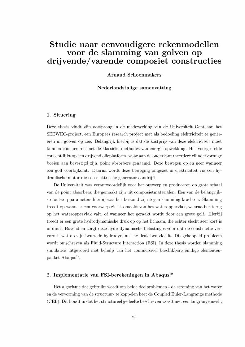
1. Situering
Deze thesis vindt zijn oorsprong in de medewerking van de Universiteit Gent aan het
SEEWEC-project, een Europees research project met als bedoeling elektriciteit te gener-
eren uit golven op zee. Belangrijk hierbij is dat de kostprijs van deze elektriciteit moet
kunnen concurreren met de klassieke methodes van energie-opwekking. Het voorgestelde
concept lijkt op een drijvend olieplatform, waar aan de onderkant meerdere cilindervormige
boeien aan bevestigd zijn, point absorbers genaamd. Deze bewegen op en neer wanneer
een golf voorbijkomt. Daarna wordt deze beweging omgezet in elektriciteit via een hy-
draulische motor die een elektrische generator aandrijft.
De Universiteit was verantwoordelijk voor het ontwerp en produceren op grote schaal
van de point absorbers, die gemaakt zijn uit composietmaterialen. Een van de belangrijk-
ste ontwerpparameters hierbij was het bestand zijn tegen slamming-krachten. Slamming
treedt op wanneer een voorwerp zich losmaakt van het wateroppervlak, waarna het terug
op het wateroppervlak valt, of wanneer het geraakt wordt door een grote golf. Hierbij
treedt er een grote hydrodynamische druk op op het lichaam, die echter slecht zeer kort is
in duur. Bovendien zorgt deze hydrodynamische belasting ervoor dat de constructie ver-
vormt, wat op zijn beurt de hydrodynamische druk beınvloedt. Dit gekoppeld probleem
wordt omschreven als Fluid-Structure Interaction (FSI). In deze thesis worden slamming
simulaties uitgevoerd met behulp van het commercieel beschikbare eindige elementen-
pakket Abaqus™.
2. Implementatie van FSI-berekeningen in Abaqus™
Het algoritme dat gebruikt wordt om beide deelproblemen - de stroming van het water
en de vervorming van de structuur- te koppelen heet de Coupled Euler-Langrange methode
(CEL). Dit houdt in dat het structureel gedeelte beschreven wordt met een langrange mesh,
vii

die de vervorming van de structuur volgt, en het fluıdum gedeelte met een euler mesh,
waarvan de knopen op dezelfde plaats blijven gedurende de simulatie. Het fluıdum stroomt
als het ware door de mesh, en het vrije vloeistofoppervlak wordt gereconstrueerd met
behulp van de Volume Of Fluid (VOF) methode. De contactformulering voor het volledige
model is ruw, wat wil zeggen dat eens er contact is tussen het fluıdum en de structuur,
het contact gesloten moet blijven. Door deze formulering te gebruiken, is er rekening
gehouden met de opwaartse Archimedeskracht. Zwaartekracht is geımplementeerd voor
het volledige model.
De fluıda worden gemodelleerd op basis van een Equation of State (EOS), en worden
beide als onsamendrukbaar beschouwd. Aangezien de optredende fluıdumsnelheden aan
de lage kant zijn bij het simuleren van slamming, is dit aanvaardbaar. Interactie tussen
verschillende euler-domeinen is niet mogelijk. Als lucht geımplementeerd wordt, moet dit
dus in hetzelfde domein gebeuren als voor het water.
3. Berekeningen met starre lichamen
Om de performantie van Abaqus™ na te gaan worden berekeningen uitgevoerd op voor-
werpen waarover informatie terug te vinden is in de internationale literatuur, zoals een
wig, een conus of een cilinder. Op deze manier kunnen de resultaten vergeleken worden
met de waarden die daar gevonden worden.
Om er voor te zorgen dat het lichaam niet vervormt tijdens de analyse, wordt een
rigid body constraint toegepast op het structurele gedeelte. Belangrijk hierbij is wel dat
randvoorwaarden, die voordien geldig waren op heel het object, of op bepaalde delen van
het object, nu moeten toegepast worden op een referentiepunt, dat een gekozen vast punt is
op het structurele gedeelte. Voor een bespreking van de randvoorwaarden wordt verwezen
naar Paragraaf 4.2.1 in de thesis. Figuur 1 geeft een overzicht van het rekendomein.
viii

Figure 1: Overzicht van rekendomein voor wig
De resultaten voor een wig werden vergeleken met een analytische uitdrukking voor de
maximum optredende druk, voorgesteld door Zhao en Faltinsen [1] (Vergelijking 1).
pmax =1
2ρV 2 π2
4tan(α)2(1)
Met ρ de dichtheid van het water, V de intredesnelheid en α de wighoek. De bekomen
resultaten voor intredesnelheid V = 5.2, m/s worden vergeleken met Vergelijking 1 in
Tabel 4.1 voor verschillende waarden van de wighoek α. De berekende drukken zijn eerder
aan de lage kant, en komen vrij goed overeen met de berekende waarden met Vergelijking
1. De afwijking wordt groter als de wighoek kleiner wordt. Wel moet opgemerkt worden
dat soms, door numerieke instabiliteiten, de waarde voor de druk in een enkel element vele
malen hoger kan liggen dan de getabelleerde waarden.
Table 1: Vergelijking tussen de berekende maximum druk en Vergelijking 1
α pmax calculated [bar] pmax Zhao [bar]
6 20.96 30.20
10 8.76 10.73
14 4.91 5.73
De resultaten voor de conus worden vergeleken met experimentele en numerieke re-
sultaten voorgesteld door Peseux et al. [2]. Opnieuw wordt een intredesnelheid van 5.2
m/s opgelegd, en de waarde van de conushoek α is 10. Een maximale druk van 10.30
bar werd berekend, terwijl Peseux [2] een maximale druk van 5.5 bar behaalde tijdens
ix

experimenten, en een waarde van 7 bar als numeriek resultaat. Er kan dus gesteld worden
dat de drukken berekend met Abaqus™zeer conservatief zijn.
Voor een cilinder en een bol werden de resultaten vergeleken met numerieke resultaten
van Battistin en Iafrati [3]. Hun resultaten zijn gegeven in de vorm van een dimensieloze
drukcoefficient Cp in functie van de dimensieloze booglengte op de cilinder y/R, voor een
bepaalde waarde van de dimensieloze onderdompeling z/R. Hierbij is R de straal van de
cilinder of de bol, en z is de onderdompeling van het structureel gedeelte. Figuur 2 toont
de drukcoefficient voor de cilinder voor zowel z = 0.01 en z = 0.05. De vorm van de
curve komt vrij goed overeen met de vorm in [3], maar de waarde voor Cp is vele malen
hoger. Voor de bol wordt hetzelfde fenomeen gezien, alhoewel de druk iets lager is door
driedimensionele effecten (Figuur 3). Ook wanneer de drukken vergeleken worden met de
experimentele resultaten van Lin en Shieh [4], blijkt dat de berekende drukken heel hoog
zijn.
0 0.05 0.1 0.15 0.2 0.25 0.3 0.35 0.4 0.45 0.5−20
0
20
40
60
80
100
120
140
160
180
y/R
Cp
z/R = 0.01z/R = 0.05
Figure 2: Dimensieloze druk voor cilinder bij verschillende waarden van z/R
x

Figure 3: Dimensieloze druk voor bol bij z/R = 0.01
Voor al deze voorwerpen werden ook simulaties uitgevoerd met de implementatie
van lucht als een tweede fase. Voor het simuleren van een onvervormbaar object, met
wighoeken groter dan 5 zou dit geen verschil mogen geven voor de resultaten: lucht
kan niet opgesloten worden in concave holtes, en de veroorzaakte weerstandskracht bij de
beschouwde snelheiden kan verwaarloosd worden ten opzichte van de zwaartekracht. De
resulterende drukken zijn echter wat lager, wat als volgt kan verklaard worden: door het
gebruik van een ruw contact, remt het object reeds af wanneer het nog in vrije val is, wat
fysisch gezien niet verwacht wordt. Daardoor is de snelheid bij impact, en dus ook de
maximale druk, lager.
Ook werd in alle simulaties een grote hoeveelheid ruis in de resulterende drukken gezien,
waarbij de druk soms extreem hoge waarden kan aannemen in een enkel element. Voor een
cilinder wordt dit geıllustreerd in Figuur 4, waar ook het optreden van een schokgolf, met
negatieve drukken waarvan de amplitude even groot kan zijn als bij de positieve drukpiek,
getoond wordt. Dit fenomeen wordt niet teruggevonden in de internationale literatuur.
xi

Figure 4: Zeer hoge druk in element door numerieke instabiliteit. Niet-uitgemiddelde waarden.
De weergave van het wateroppervlak bij de impact van een cilinder wordt vergeleken met
experimentele resultaten van Lin en Shieh [4], die een hoge-snelheids camera gebruikten
om de vorming van de jet vast te leggen. In de simulatie met Abaqus™ wordt de vorm
en de richting van de jet vrij goed benaderd, enkel het aantal druppeltjes dat zich vormt
ligt lager. Dit is te wijten aan het feit dat de kleinste van deze druppeltjes niet opgelost
worden in de mesh.
(a) t = 0.0285 − 0.0342s (rising up) (b) t = 0.03s (rising up)
xii

4. Berekeningen met vervormbare lichamen
De optredende drukken zijn lager wanneer de vervorming in rekening wordt gebracht,
en het deel van het object dat op het water slamt ondervindt een grotere deceleratie. Voor
de wig is de maximum optredende druk gelijk aan 8.64 bar. Ook hier worden ietwat lagere
drukken bekomen wanneer lucht geımplementeerd wordt, maar de invloed van lucht is
groter door de vervorming. Aangezien de gebruikte wighoek groot genoeg is om cushioning
(waarbij lucht vastgeraakt in concave holtes onder het voorwerp) te voorkomen, kan hieruit
geconcludeerd worden dat lucht toch enigzins vastgeraakt, wat er op kan wijzen dat lucht
te stijf gemodelleerd is.
Figuur 5 toont de druk in het element waar de eerste impact plaats vindt, in functie van
de tijd en voor verschillende waarden van α. Om de figuur wat duidelijker te maken, werd
aan de curves een zekere offset in de x-richting meegegeven. In Tabel 2 is een vergelijking
gemaakt met experimentele en numerieke resultaten van Peseux [2] voor een vervormbare
conus. Ook hier blijkt dat de berekende drukken hoger zijn dan verwacht.
0 1 2 3 4 5 6 7
x 10−4
−8
−6
−4
−2
0
2
4
6
8
Time [s]
Pressure [bar]
! = 6°! = 10°! = 14°
Figure 5: Druk in element waar eerste impact plaats heeft, voor verschillende waarden van α
xiii

Table 2: Vergelijking van resultaten van Peseux [2] met berekende resultaten voor vervormbare
conus
α Peseux Experimental [bar] Peseux Numerical [bar] Abaqus™[bar]
6 1.4 2.2 6.67
10 1.2 1.3 4.83
14 0.6 0.6 3.66
Omdat de point absorbers uit glasvezel versterkte composiet gemaakt zijn, zijn ook simu-
laties voor een cilinder met hetzelfde materiaal uitgevoerd, en vergeleken met de resultaten
voor dezelfde cilinder gemaakt uit staal (ρ = 7800 kg/m3, E = 210GPa, ν = 0.3). Beide
cilinders hebben een dikte van 3 mm. De vervorming voor zowel een stalen als een com-
posiet cilinder is weergegeven in Figuur 6. Let wel dat hier een schalingsfactor 20 is
gebruikt om de vervorming te kunnen visualiseren. In werkelijkheid blijft het onderste
punt van de cilinders het onderste punt gedurende de analyse, zodat eigenlijk een ellip-
tische vervorming verkregen wordt. De procentuele afwijking van de originele diameter
wordt getoond in Figuur 7. Voor een stalen cilinder is de afwijking op het einde van de
simulatie 1.29%, voor een composiet cilinder 2.05%, wat te verklaren is door de grotere
stijfheid van het staal.
xiv

(a) staal (b) composiet
Figure 6: Vervorming voor stalen en composiet cilinder. t na impact is 1.25 ms
0 0.5 1 1.5 2 2.5
x 10−3
0
0.2
0.4
0.6
0.8
1
1.2
1.4
Time [s]
DOD [%]
(a) staal
0 0.5 1 1.5 2 2.5
x 10−3
0
0.5
1
1.5
2
2.5
Time [s]
DOD [%]
(b) composiet
Figure 7: Procentuele afwijking van originele diameter
Aangezien de stijfheid van het composiet materiaal lager is, treedt er grotere vervorming
op, wat ook tot een lagere druk leidt. Figuur 8 toont Cp voor een stalen cilinder. De waar-
den van de dimensieloze onderdompeling zijn z/R=0.01 en z/R=0.05. De drukcoefficient
Cp is lager dan voor een starre cilinder, maar is nog steeds veel hoger dan de waarden
gevonden in [3]. Ook komt de vorm van de curve minder overeen door het optreden van
grote schommelingen in de druk.
xv

0 0.05 0.1 0.15 0.2 0.25 0.3 0.35 0.4 0.45 0.5−40
−20
0
20
40
60
80
100
120
140
160
y/R
Cp
z/R = 0.01z/R = 0.05
Figure 8: Dimensionless pressure for deformable cylinder
Om te kijken of het composietmateriaal zou falen bij de impact, werd het Tsai-Wu
criterium toegepast. Dit is een schadecriterium dat gebaseerd is op de spanningstoestand
in het materiaal, bepaald door σ11, σ22, σ12. Om niet beschadigd te geraken, mag de
Tsai-Wu waarde IF niet groter worden dan 1. Voor de onderste en bovenste laag is de
waarde van IF weergeven in Figuur 9. Omdat de cilinder buiging ondergaat, zijn dat de
twee meest bepalende lagen. Zoals te zien op de figuur blijft IF overal kleiner dan 1, en de
zones waar de cilinder het water raakt zijn het meest kritiek. De spanningen veroorzaakt
door de vervorming zijn dus echter te klein om schade te veroorzaken.
xvi

(a) onderste laag (b) bovenste laag
Figure 9: Tsai-Wu failure criterion
5. Conclusie
De performantie van Abaqus™ om FSI-berekeningen uit te voeren bij hydrodynamische
impact is onderzocht. De vervorming van de objecten geeft aanleiding tot een lagere druk,
maar de waarden voor de maximale druk zijn toch groter dan de waarden die gevonden
zijn in de internationale literatuur. Op sommige tijdstippen wordt de druk in een bepaald
element van de mesh extreem hoog. Bovendien heeft te implementatie van lucht als een
tweede fase een grotere invloed heeft dan verwacht: het object wordt al afgeremd door de
lucht terwijl het nog in vrije val is. Ook heeft de lucht een grotere invloed bij vervormbare
objecten waarvoor geen cushioning effect verwacht wordt, wat er op kan wijzen dat lucht
te stijf gemodelleerd is.
xvii

Contents
Contents xviii
1 Introduction 1
1.1 Introduction . . . . . . . . . . . . . . . . . . . . . . . . . . . . . . . . . . . . 1
1.2 The SEEWEC-project . . . . . . . . . . . . . . . . . . . . . . . . . . . . . . 1
1.3 Slamming . . . . . . . . . . . . . . . . . . . . . . . . . . . . . . . . . . . . . 2
1.4 Goal of the thesis . . . . . . . . . . . . . . . . . . . . . . . . . . . . . . . . . 4
1.5 Structure of the thesis . . . . . . . . . . . . . . . . . . . . . . . . . . . . . . 4
2 Literature Study 5
2.1 Introduction . . . . . . . . . . . . . . . . . . . . . . . . . . . . . . . . . . . . 5
2.2 Analytical Models . . . . . . . . . . . . . . . . . . . . . . . . . . . . . . . . 5
2.2.1 Early Investigations . . . . . . . . . . . . . . . . . . . . . . . . . . . 5
2.2.2 Recent developments . . . . . . . . . . . . . . . . . . . . . . . . . . . 6
2.3 Numerical models . . . . . . . . . . . . . . . . . . . . . . . . . . . . . . . . . 10
2.3.1 Recent developments . . . . . . . . . . . . . . . . . . . . . . . . . . . 12
2.3.2 Fluid-Structure Interactions (FSI) . . . . . . . . . . . . . . . . . . . 14
2.3.3 Volume Of Fluid Method (VOF) . . . . . . . . . . . . . . . . . . . . 18
3 Implementation of a CEL-model in Abaqus™/CAE 22
3.1 Introduction . . . . . . . . . . . . . . . . . . . . . . . . . . . . . . . . . . . . 22
3.2 Explicit dynamic analysis . . . . . . . . . . . . . . . . . . . . . . . . . . . . 22
3.2.1 Properties . . . . . . . . . . . . . . . . . . . . . . . . . . . . . . . . . 22
3.2.2 Stable increment time . . . . . . . . . . . . . . . . . . . . . . . . . . 23
3.2.3 Application to CEL . . . . . . . . . . . . . . . . . . . . . . . . . . . 24
3.3 Material definitions . . . . . . . . . . . . . . . . . . . . . . . . . . . . . . . . 24
3.4 Contact interactions . . . . . . . . . . . . . . . . . . . . . . . . . . . . . . . 26
3.5 Predefined fields . . . . . . . . . . . . . . . . . . . . . . . . . . . . . . . . . 27
3.6 Boundary conditions and loads . . . . . . . . . . . . . . . . . . . . . . . . . 28
xviii

Contents
3.7 Mesh . . . . . . . . . . . . . . . . . . . . . . . . . . . . . . . . . . . . . . . . 28
3.7.1 Displacement hourglass scaling factor s . . . . . . . . . . . . . . . . 29
3.7.2 Bulk viscosity scaling factors b1 and b2 . . . . . . . . . . . . . . . . . 29
3.7.3 Mesh size . . . . . . . . . . . . . . . . . . . . . . . . . . . . . . . . . 30
4 Calculations for rigid bodies 31
4.1 Introduction . . . . . . . . . . . . . . . . . . . . . . . . . . . . . . . . . . . . 31
4.2 Wedge . . . . . . . . . . . . . . . . . . . . . . . . . . . . . . . . . . . . . . . 31
4.2.1 Introduction . . . . . . . . . . . . . . . . . . . . . . . . . . . . . . . 31
4.2.2 Results . . . . . . . . . . . . . . . . . . . . . . . . . . . . . . . . . . 35
Effect of deadrise angle α . . . . . . . . . . . . . . . . . . . . . . . . 40
Influence of the implementation of air . . . . . . . . . . . . . . . . . 43
4.3 Cone . . . . . . . . . . . . . . . . . . . . . . . . . . . . . . . . . . . . . . . . 46
4.3.1 Introduction . . . . . . . . . . . . . . . . . . . . . . . . . . . . . . . 46
4.3.2 Results . . . . . . . . . . . . . . . . . . . . . . . . . . . . . . . . . . 49
Pressure . . . . . . . . . . . . . . . . . . . . . . . . . . . . . . . . . . 49
Comparison with experimental results . . . . . . . . . . . . . . . . . 51
4.4 Cylinder . . . . . . . . . . . . . . . . . . . . . . . . . . . . . . . . . . . . . . 52
4.4.1 Introduction . . . . . . . . . . . . . . . . . . . . . . . . . . . . . . . 52
4.4.2 Results . . . . . . . . . . . . . . . . . . . . . . . . . . . . . . . . . . 54
Implementation of air . . . . . . . . . . . . . . . . . . . . . . . . . . 59
Comparison with experimental results . . . . . . . . . . . . . . . . . 60
Comparison with numerical model . . . . . . . . . . . . . . . . . . . 62
Formation of the jet . . . . . . . . . . . . . . . . . . . . . . . . . . . 63
Conclusion . . . . . . . . . . . . . . . . . . . . . . . . . . . . . . . . 66
4.5 Sphere . . . . . . . . . . . . . . . . . . . . . . . . . . . . . . . . . . . . . . . 66
4.6 Conclusion . . . . . . . . . . . . . . . . . . . . . . . . . . . . . . . . . . . . 68
5 Calculations on deformable bodies 70
5.1 Introduction . . . . . . . . . . . . . . . . . . . . . . . . . . . . . . . . . . . . 70
5.2 Wedge . . . . . . . . . . . . . . . . . . . . . . . . . . . . . . . . . . . . . . . 70
5.2.1 Introduction . . . . . . . . . . . . . . . . . . . . . . . . . . . . . . . 70
5.2.2 Results . . . . . . . . . . . . . . . . . . . . . . . . . . . . . . . . . . 71
Deformation . . . . . . . . . . . . . . . . . . . . . . . . . . . . . . . 71
Pressure . . . . . . . . . . . . . . . . . . . . . . . . . . . . . . . . . . 72
5.3 Cone . . . . . . . . . . . . . . . . . . . . . . . . . . . . . . . . . . . . . . . . 75
5.3.1 Introduction . . . . . . . . . . . . . . . . . . . . . . . . . . . . . . . 75
xix

Contents
5.3.2 Results . . . . . . . . . . . . . . . . . . . . . . . . . . . . . . . . . . 76
Pressure . . . . . . . . . . . . . . . . . . . . . . . . . . . . . . . . . . 76
5.4 Cylinder . . . . . . . . . . . . . . . . . . . . . . . . . . . . . . . . . . . . . . 78
5.4.1 Introduction . . . . . . . . . . . . . . . . . . . . . . . . . . . . . . . 78
5.4.2 Results . . . . . . . . . . . . . . . . . . . . . . . . . . . . . . . . . . 78
Deformation . . . . . . . . . . . . . . . . . . . . . . . . . . . . . . . 78
Pressure . . . . . . . . . . . . . . . . . . . . . . . . . . . . . . . . . . 81
5.4.3 Composite cylinder . . . . . . . . . . . . . . . . . . . . . . . . . . . . 83
Modelling of the composite lay-up . . . . . . . . . . . . . . . . . . . 83
5.4.4 Results . . . . . . . . . . . . . . . . . . . . . . . . . . . . . . . . . . 85
Deformation . . . . . . . . . . . . . . . . . . . . . . . . . . . . . . . 85
Pressure . . . . . . . . . . . . . . . . . . . . . . . . . . . . . . . . . . 88
Failure of the material . . . . . . . . . . . . . . . . . . . . . . . . . . 88
5.5 Conclusion . . . . . . . . . . . . . . . . . . . . . . . . . . . . . . . . . . . . 91
6 Conclusion 93
Bibliography 95
List of Figures 98
List of Tables 102
xx

Nomenclature
Abbreviations
CEL Coupled Euler-Lagrange
DOD Deviation of Original Diameter
FSI Fluid Structure Interaction
SEEWEC Sustainable Economically Efficient Wave Energy Converter
VOF Volume Of Fluid
WEC Wave Energy Converter
Units
α Deadrise angle
c0 wave speed in material m/s
Cp Pressure coefficient -
E Elastic modulus Pa
G Shear modulus Pa
M Mass kg
µ Dynamic viscosity Pa · s
ν Poisson ratio -
p Pressure Pa
R Radius of cylinder/sphere m
ρ Density kg/m3
s Stress tensor Pa
σ11 Stress in fibre direction Pa
σ22 Stress perpendicular to fibre direction Pa
σ12 Shear stress Pa
v Velocity m/s
V Impact velocity m/s
y Arc length on cylinder/sphere m
z Penetration depth m
Chapter 1
Introduction
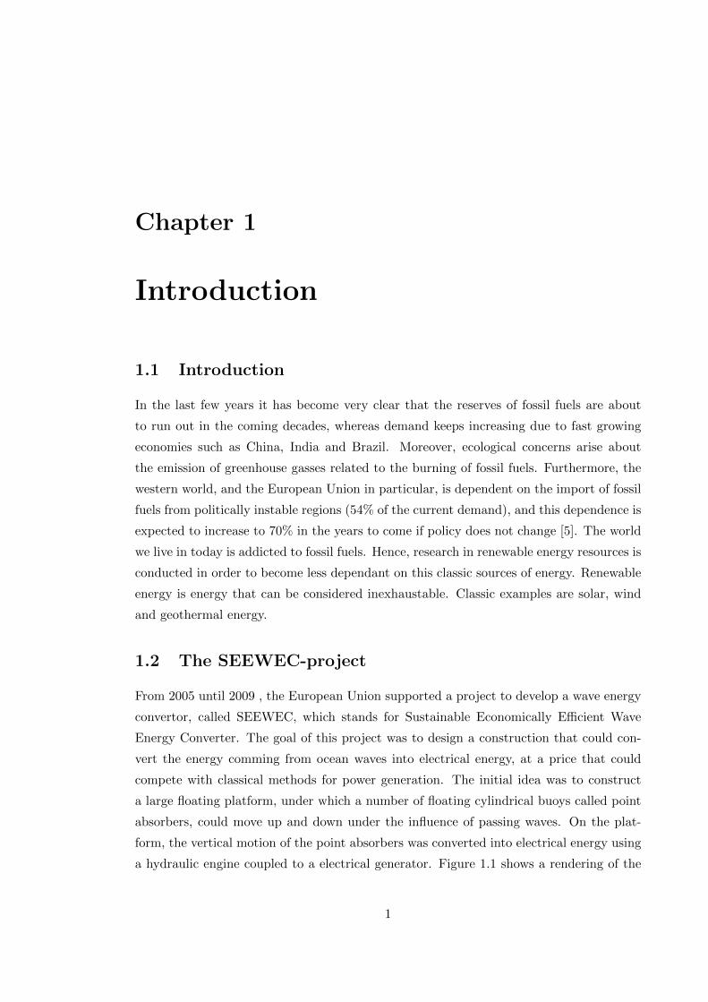
1.1 Introduction
In the last few years it has become very clear that the reserves of fossil fuels are about
to run out in the coming decades, whereas demand keeps increasing due to fast growing
economies such as China, India and Brazil. Moreover, ecological concerns arise about
the emission of greenhouse gasses related to the burning of fossil fuels. Furthermore, the
western world, and the European Union in particular, is dependent on the import of fossil
fuels from politically instable regions (54% of the current demand), and this dependence is
expected to increase to 70% in the years to come if policy does not change [5]. The world
we live in today is addicted to fossil fuels. Hence, research in renewable energy resources is
conducted in order to become less dependant on this classic sources of energy. Renewable
energy is energy that can be considered inexhaustable. Classic examples are solar, wind
and geothermal energy.
1.2 The SEEWEC-project
From 2005 until 2009 , the European Union supported a project to develop a wave energy
convertor, called SEEWEC, which stands for Sustainable Economically Efficient Wave
Energy Converter. The goal of this project was to design a construction that could con-
vert the energy comming from ocean waves into electrical energy, at a price that could
compete with classical methods for power generation. The initial idea was to construct
a large floating platform, under which a number of floating cylindrical buoys called point
absorbers, could move up and down under the influence of passing waves. On the plat-
form, the vertical motion of the point absorbers was converted into electrical energy using
a hydraulic engine coupled to a electrical generator. Figure 1.1 shows a rendering of the
1

Chapter 1. Introduction
wave energy convertor (WEC).
Figure 1.1: WEC platform concept
Several partners were chosen to design different aspects of the project, of which Ghent
University was responsable for the composite material design and the large scale manufac-
turing of the point absorbers. One of the most important design criteria was the durability
of the point absorbers, as violent waves can cause severe loads during heavy storms.
1.3 Slamming
The point absorbers must be designed in order not to fail under slamming loads. Slamming
occurs when a structure, for example a ship, is released from the water surface after which
it hits the water surface again. The object is then exposed to a hydrodynamic impact (see
Figure 1.2). The same phenomenon occurs when a structure, for example an oil rig, is hit
by a large wave. Slamming is characterized by a high pressure load that is very short in
time, but can cause severe damage to the structure. Moreover, in several cases, slamming
is identified as the cause of failure of ships and floating structures [2]. Because of this,
slamming research is mainly focused on marine applications.
2

Chapter 1. Introduction
Figure 1.2: Slamming of composite hull during the 2008 Volvo Ocean Race
The pressure distribution on a object that impacts a water surface is characterized by
a large and small pressure peak, as can be seen on Figure 1.3. Point absorbers can be
exposed to the same kind of load when they are released from the water surface and slam
back onto it. This can be caused by a resonance of the vertical movement of the point
absorber with the passing wave, in which the wave amplifies the motion of point absorber,
or when there is a phase shift between the movement of the point absorbers and the wave,
meaning that the point absorber moves down when the water surface rises, or vice versa.
In order to remain operative for several years and thus survive sometimes severe storms,
the magnitude of the occuring pressures must be known precisely to select a material
with the appropriate characteristics. This is rather complex, because the pressure has an
influence on the deformation of the structure, which in return influences the flowfield and
the pressure; this coupled problem is referred to as Fluid-Structure Interaction (FSI).
3

Chapter 1. Introduction
Figure 1.3: Pressure distribution on an impacting wedge [6]
1.4 Goal of the thesis
A numerical approach to solve Fluid-Structure Interactions was presented in a previous
thesis by Koen Stoop and Steve Vermeulen [7]. They simulated slamming events using
a coupling algorithm between Fluent™, which is a fluid solver, and Abaqus™, which is a
structural solver, to simulate slamming events. The pressures calculated with Fluent™ are
implemented on the structure in Abaqus™, which results in a deformation of the structure.
This deformation is then implemented back in Fluent™.
However, since the release of version 6.7 of Abaqus™, it is possible to include fluids in
the simulations, using only Abaqus™. The goal of this thesis is to assess the performance
of Abaqus™ for modelling slamming situations, which is done by comparing the results
from these calculations with results presented in international literature. In this thesis,
the Extended Functionality version 6.9-EF is used.
1.5 Structure of the thesis
First, a history of the research conducted on hydrodynamic impact is presented, and the
most important models, both analytical and numerical, are discussed. Next, the model
parameters of the simulation in Abaqus™ are explained, and the choice for the values
of those parameters is argumented. The results of calculations on rigid objects, such as
wedges and cylinders, are given in Chapter 4. In Chapter 5, the results for calculations
on deformable objects is presented, where both steel and composite materials are used as
materials for the impacting objects. Finally, a conclusion about the obtained results is
given in Chapter 6.
4

Chapter 2
Literature Study
2.1 Introduction
Hydrodynamic impact is a problem which is hard to solve analytically, because the solution
is highly dependent on the shape of the water close to the impacting object. Moreover,
boundary conditions must be applied to the water surface of which the position is not
known. This makes the slamming problem a highly non-linear phenomenon. In this
chapter a brief history of the research in the field of hydrodynamic impact is presented.
Both analytical as well as numerical models are discussed.
2.2 Analytical Models
2.2.1 Early Investigations
One of the first persons to investigate the slamming phenomenon was Theodore Von
Karman [8]. In 1932 he developed an analytical formula based on the conservation of
momentum, in order to estimate the forces on a seaplane when it lands on the water
surface. When an object hits the water it slows down; if momentum is to remain constant,
this means that the mass has to increase: MV = (m + M)v, with V the initial impact
velocity and m the added or virtual mass [9]. Newman [10] states that “The added mass
can be interpreted as a particular volume of fluid particles that are accelerated with the
body.” When differentiating the momentum equation with respect to time, the impact
force and pressure can be calculated. The accuracy of this method depends on the choice
of the value of the added mass. Von Karman assumed the added mass to be one half of
the inertia of a flat plat accelerated in a liquid, because the fluid underneath the plate is
accelerated, but the fluid above is not. With this assumptions, Von Karman obtained an
5

Chapter 2. Literature Study
expression for the maximum pressure at impact pmax (Equation 2.1) which is suitable for
a two-dimensional wedge on a flat water surface with an impact velocity V .
pmax =ρV 2
2πcot(α) (2.1)
α is the angle between the water surface and the wedge, called the deadrise angle (Figure
2.1), and ρ is the density of the water.
Figure 2.1: Definition of the deadrise angle α
The influence of the dynamic pressure due to the velocity, ρV 2/2 and the influence of
the shape, πcot(α), can clearly be distinguished. Furthermore, Von Karman neglects the
buoyancy, friction and the cushioning effect of air. Water elevation is also not considered,
which results in an underestimation of the pressure.
Wagner [11] expanded Von Karmans theory to two-dimensional wedges with small deadrise
angles, including the effect of the water pile-up and the spray thickness. He used an
incompressible potential flow to describe the problem. A lot of correction factors were
later added to Wagner formula’s, to include three-dimensional effects and larger deadrise
angles amongst other things.
The first person to experimentally investigate slamming is Watanabe [9]. In two papers
[12, 13] he describes experimental drop tests of cones with variable deadrise angle and
impact velocity and the resulting impact force. Such experimental results were extremely
important to validate the at that time recently developed analytical models.
2.2.2 Recent developments
Zhao et al. [1] derived an analytical expression for the pressure distribution on a body by
further developing Wagner’s theory, also using an incompressible and inviscid potential
6

Chapter 2. Literature Study
flow. It is valid for small deadrise angles higher than 2, so the cushioning effect of air can
be neglected.
An expression for a slamming coefficient Cpmax is proposed:
Cpmax ≡pmax12ρV
2=
π2
4tan(α)2(2.2)
They also show that the global pressure distribution is not much influenced by the local
jet of water, which arises on the side of the impacting object.
Inspired by the work of Zhao [1], an analytical expression for the pressure on general two-
dimensional sections was developed by Mei et al. [14]. They generalize Wagners method
to a various range of body sections, and use the same initial-boundary-formulation as in
the work of Zhao [1] in which the pressure at the free surface is set to zero. Moreover,
the expression can be solved analytically for wedges and cylinders, in contrary to Zhao’s
expression, which can only be solved with numerical aid. Expressions for more general
ship sections are also derived. However, for three-dimensional objects, the expressions are
limited to a number of geometric shapes.
The pressure coefficient Cp(y, t) ≡ P (y, t)/(ρV2
2 ), y ≤ Y (t) is given by:
Cp(y, t) =2γ
A tan(α)
[(1− q2
q2
)θ ∫ 1
|q|
(w2
1− w2
)θdw − q
]−(
1− q2
q2
)2θ
− 2γ+ 1 (2.3)
In this equation:
• q is related to the position of the impacting object:
h(y)
V t= γA−1cos(β)
∫ q
0
(w2
1− w2
)θdw + γ (2.4)
• h(y) is the height on the impacting object
• vt is the submersion of the body, where v is the actual velocity and t is the time
after impact
• A, θ and γ are constants, depending on the deadrise angle.
Figure 2.2 gives an overview of the used definitions.
7

Chapter 2. Literature Study
Figure 2.2: Slamming definitions
The results obtained by Mei [14] for wedges with different deadrise angles α are shown
in Figure 2.3, in which the influence of the deadrise angle is clearly visible: a smaller
angle gives a higher and shorter pressure peak, a large angle gives a lower and wider
pressure peak. This can be understood intuitively, because a sharper object cuts more
easily through the water. Furthermore, In Figure 2.3, a comparison is made with the
similarity solution obtained by Dobrovol’Ska [15], represented by the dotted line.
8

Chapter 2. Literature Study
Figure 2.3: Solution for a wedge obtained by Mei for several deadrise angeles. Comparison with
the similarity solution obtained by Dobrovol’Skaya.
These expressions are derived based on the conservation of momentum. In 1951, Pierson
[16] noticed that when the concept of added mass is used in an energy-based analysis,
different results are obtained. However, Cointe et al. [17], proved that when the energy
flux going into the water jet is taken into account, the results are the same as when
9

Chapter 2. Literature Study
conducting a momentum-based analysis.
2.3 Numerical models
The governing equations for fluid flow are the Navier-Stokes equations: conservation of
mass (Equation 2.5), momentum-equation (Equation 2.6) and energy-equation (Equation
2.7). These equations are not solvable in an analytical way.
∂ρ
∂t+∇ · (ρv) = 0 (2.5)
ρ∂v
∂t+ ρv ·∇(v) = ∇ · s + f (2.6)
ρ∂e
∂t+ ρv ·∇(e) = s : ∇(v) + f ·v (2.7)
The parameters in these equations are as follows:
• f is the external force density.
• v is the velocity vector
• The total Cauchy stress s is given by:
s = −p · I + µ(∇(v) +∇(v)T ) (2.8)
where p is the pressure and µ represents the dynamic viscosity
Together with the initial- and boundary conditions, these equations completely determine
the flow. For the slamming problem, two different regions on the boundary of the domain
are distinguished (Figure 2.4):
• The velocity is prescribed on ∂Ω1f : ·v(t) = g(t)
• The velocity isn’t prescribed, but the traction boundary condition is assumed to be
imposed on ∂Ω2f : · s ·n = h(t)
10

Chapter 2. Literature Study
Figure 2.4: Fluid domain
When computers became powerful enough to solve large sets of equations, a lot of nume-
rical slamming models were developed. The Navier-Stokes equations were formulated in
a discrete form and solved numerically.
A lot of these numerical models are based on a mixed Euler-Lagrangian formulation.
Longuet-Higgings and Cokelet [18] first proposed this method in 1979. The flow velocity
potential is solved with Dirichlet boundary conditions on the free surface, and Neumann
boundary conditions on the solid body. The solution gives the velocity along the body
contour and, by deriving in the normal direction, the normal derivative on the free surface,
meaning the velocity components on the free surface are then known. By integrating the
velocity with respect to time, the position of the free surface is known. Applying the
Bernoulli-equation for an unsteady flow (∂v∂t 6= 0) results in the velocity potential along
the free surface. The problem with this method is that, after discretisation, the boundary
conditions on the intersection of the free surface and the solid body do not match, causing
a flow singularity, see Figure 2.5. A very fine jet appears, characterized by a large velocity
gradient. This results in an unreliable, very high pressures at first impact, located in the
spray root.
11

Chapter 2. Literature Study
Figure 2.5: Boundary conditions in computational domain.
2.3.1 Recent developments
Battistin and Iafrati [3] developed a numerical model dealing with these issues, applied
to axisymmetric objects. The very fine jet is cut out of the computational domain, once
the distance between the first centroid on the free surface and the rigid body reaches a
fixed treshold value. This still leads to reliable results, because in spite of the high kinetic
energy of the jet, only a small changes of the pressure field occurs in this region[17]. Iafrati
et al. [19] validated that model for axisymmetric wedges. A similar model was suggested
by Zhao and Faltinsen [1].
Figure 2.6: Cut-off jet in computational domain
Peseux et. al [2] developed a model to solve the three-dimensional Wagner problem numer-
ically, both for rigid as well as for deformable structures. The potential flow assumptions
12

Chapter 2. Literature Study
are valid: the fluid is inviscid, incompressible and irrotational. The domain is divided into
three different zones, as can be seen in Figure 2.7.
Figure 2.7: Definition of different domains in computational domain
In each of these domains an asymptotic expansion is performed. The first one is the
outer domain. Here, the solution resembles the flow obtained around a flat plate that is
immersed in a fluid, which is referred to as the outer problem. Next, the spray source
domain near the contact line, where the flow overturns to create a jet, is considered: this is
called the inner problem. The last zone, the jet domain, is not considered to influence the
solution and is not taken into account. A variational formulation of the Wagner problem is
developed both for two-dimensional and three-dimensional slamming problems. To solve
these equations, a finite element method was conceived. Moreover, a series of experimental
slamming tests with cones, both deformable and undeformable and with different deadrise
angles, were performed to compare with the obtained numerical results shown in Figure
2.8. Here, the pressure is shown for 4 different timesteps in the analysis, with t1 < t4. The
displacement of the pressure peak along the wedge in time can clearly be seen.
13

Chapter 2. Literature Study
Figure 2.8: Comparison between cone and wig with same deadrise angle of 10at 4 different
timesteps. Impact velocity is 6m/s
2.3.2 Fluid-Structure Interactions (FSI)
The first models considered the impacting objects as rigid bodies. In real-life slamming
events, some deformation of the structure occurs. This deformation influences the flow
around the object and also the pressures. In general, the pressures are lower, because
air gets trapped in concave cavities. This is called the cushioning effect, as illustrated in
Figure 2.9.
14

Chapter 2. Literature Study
Figure 2.9: Air gets trapped in concave cavities when the impacting object deforms. The air is
compressed and the object slows down.
Equation 2.9 governs the deformation of the structure. It expresses the conservation of
momentum.
ρdv
dt= ∇(s) + f (2.9)
Two boundary conditions are applied (Figure 2.10):
• The displacement boundary condition on ∂Ωs1 : x(X, t) = D(t). Here, x(t) is the
displacement, X represents the reference coordinates X1, X2 and X3.
• The traction boundary condition on ∂Ωs2 : s ·n = τ (t). n is the normal orientated
outward on ∂Ωs2.
Figure 2.10: Structural domain
When the deformation of the structure is also taking into account, contact algorithms
must be developed to calculate the contact forces applied from the fluid to the structure
and vice versa. An explicit method is used to update the nodal forces at the interface
15
Chapter 2. Literature Study
each time step to calculate the contact forces. To stay in contact with the structure, fluid
nodes must follow the structure at the interface. Souli and Zolesio [20] and Rabier and
Medale [21] present a coupling algorithm where remeshing is not applied. Only small fluid
motions are allowed in order to prevent mesh distortion, as this would lead to incorrect
results. When modeling fluids with such a mesh, the mesh gets severely distorted due to
the large deformations of the water, as can be seen in Figure 2.11(a). A remeshing method
is needed, which is very CPU-time consuming.
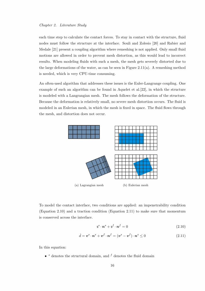
An often-used algorithm that addresses these issues is the Euler-Langrange coupling. One
example of such an algorithm can be found in Aquelet et al.[22], in which the structure
is modeled with a Langrangian mesh. The mesh follows the deformation of the structure.
Because the deformation is relatively small, no severe mesh distortion occurs. The fluid is
modeled in an Eulerian mesh, in which the mesh is fixed in space. The fluid flows through
the mesh, and distortion does not occur.
(a) Lagrangian mesh (b) Eulerian mesh
To model the contact interface, two conditions are applied: an impenetrability condition
(Equation 2.10) and a traction condition (Equation 2.11) to make sure that momentum
is conserved across the interface.
ss ·ns + sf ·nf = 0 (2.10)
d = vs ·ns + vf ·nf = (vs − vf ) ·ns ≤ 0 (2.11)
In this equation:
• s denotes the structural domain, and f denotes the fluid domain
16
Chapter 2. Literature Study
• d is the penetration vector
• s is the total Cauchy stress (Equation 2.8)
• n is the normal on the domain boundary
The interaction itself can be modeled in different ways. One surface (either fluid or
structural) is the master surface, the other one is the slave surface, containing the slave
nodes. Kinematic contact, where fluid and structure have te same velocity, makes sure
momentum is conserved, but violates the energy equation. Another possibility is to apply
the penalty based method. A penalty is a resisting force to the slave node, dependent
on its penetration through the master node. To satisfy equilibrium, an opposite force is
applied to the nodes of the master element. In Aquelet [22] an expression for the forces is
proposed:
Fs = −k · d (2.12)
F im = Ni · k · d (2.13)
Ni is a shape function at node i. This can be interpreted as springs with stiffness k placed
between the slave nodes and the contact surface, see Figure 2.11. The stiffness depends
on the bulk modulus K of the master material, the surface area A of the master element
and the volume V of the master element:
k = pfKA
V(2.14)
where pf is scale factor for the interface stiffness. It must satisfy 0 ≤ pf ≤ 1.
17

Chapter 2. Literature Study
Figure 2.11: Contact algorithm
2.3.3 Volume Of Fluid Method (VOF)
When using an Euler-Lagrange coupling, the fluid is modeled with a fixed mesh. The
location of the free surface cannot be calculated by looking at the displacement of the
nodes. Therefore, a different approach is needed to determine the free surface; several
methods exist:
In the level-set free surface tracking method, the distance function φ(x, t) is introduced
to know the distance of the surface x from its initial position at t = 0. The interface
corresponds to φ(x, t) = 0. The problem with this model is that mass is not conserved.
The most popular model is the Volume of fluid model (VOF) [23]. The volume fraction F
is the fractional volume of a cell occupied by the fluid, and has a value between zero and
one. Every cell has its own VOF. Cells with F = 0 or F = 1 are called pure cells; when
0 ≤ F ≤ 1, the cell is called a mixed cell. The VOF-method was first introduced by Hirt
and Nichols [24]. It has two important characterizing properties: The way the interface
is reconstructed and the way it is propagated. As explained later on in this section,
several methods exist to reconstruct the interface. Based on the obtained interface and
the velocity fluxes at the different surfaces of each cell, fluid is moved from a donor cell
to an acceptor cell. Only the value of the VOF in surrounding cells is needed to calculate
the VOF in cell. This makes it easy to divide the calculations in parallel processes.
Rider [25] identifies 4 steps to calculate the VOF, as shown in Figure 2.12. In the first step,
18

Chapter 2. Literature Study
the volume is divided in descrete parts using a mesh. Next, the free surface is discretised.
Now the material fluxes can be calculated. In the final step, the volumes are integrated
to a new time level.
Figure 2.12: Steps taken to calculate Volume Fraction F
Two ways of reconstructing the surface are much used nowadays. First, there is the Simple
Line Interface Calculation method (SLIC), where the interface is always parallel to one of
the coordinate axes. As can be seen in Figure 2.13(a), this method is not very accurate.
A more sophisticated method is the Piecewise Linear Interface Reconstruction method
(PLIC), as can be seen in Figure 2.13(b). To reconstruct the interface, it is divided by a
19

Chapter 2. Literature Study
line in a certain number of discrete partitions equal to the number of phases present in
the cell. The line is a linear approximation of the curved interface. Also, a discontinuity
between the different lines is allowed. This method is very accurate when the curvature
of the interface is small, but even when the fluid surface has a large curvature it remains
robust. This is important especially when modelling events which can contain droplets,
because infinite curvatures may appear when these droplets reconnect.
(a) SLIC (b) PLIC
Figure 2.13: Comparison between the SLIC and PLIC surface reconstruction algorithms
The advection equation that governs F for an incompressible fluid can be written as follows
[25]:
∂F
∂t+ u ·∇F → ∂F
∂t+∇ · (uF ) = 0 (2.15)
where u is the flowfield. This equation shows that volume is conserved along a streamline.
The fluxes through a cell face can be calculated using:
∂F = u ·nA∂t. (2.16)
WithA the cell surface and ∂t the time step.
When these fluxes are calculated, the VOF is updated from level n to n+ 1:
Fn+1 = Fn +∂Fe + ∂Fn − ∂Fw − ∂Fs
∂x∂y. (2.17)
20

Chapter 2. Literature Study
The indices n, e, s and w stand for north, east, south and west, representing the fluxes
through the different faces of a cell in two dimensions. Away from the free surface, the
net flux becomes zero. Around the free surface the calculation of the fluxes becomes more
complicated, a method to do so can be found in Hurt and Nichols [24].
There are however some major drawbacks to this method. First of all, conservation of mass
may be violated when rounding F when F ≤ 0 or F ≥ 1 [23]. Further, a lot of droplets
that disconnect from the surface may appear, which is called flotsam or jetsam. This is
especially the case for the lower-order methods like SLIC [25]. To address these problems,
a local height function was introduced. A detailed description is given by Gerrits [26]. The
local height function h is defined in each surface cell, and gives the height of the surface
in a column of three cells each. The direction of the local height function is defined as the
direction most normal to the free surface.
Figure 2.14: Local height function h
Normally, when the fluxes at the boundaries are calculated, the individual values of the
VOF are updated. Here the local height function h is updated instead. Afterwards, the
VOF is calculated from the height of the fluid in each column. No underflow or overflow
of the column can appear, so this method is strictly mass conserving. Also, the amount
of flotsam or jetsam is much smaller, which is physically more correct. As a conclusion,
it can be stated that the introduction of the local height function definitely improves the
performance of the VOF algorithm.
21

Chapter 3
Implementation of a CEL-model
in Abaqus™/CAE
3.1 Introduction
Simulia, the company that develops Abaqus™, gives a detailed description of what is
needed to build a Coupled Euler-Lagrang (CEL) model, but no explanation is given about
why it is necessary to adjust certain features or parameters to a certain value. The goal
of this chapter is to explain the principles behind the construction of a CEL-model.
3.2 Explicit dynamic analysis
3.2.1 Properties
In order to simulate slamming events, a dynamic analysis is needed. In Abaqus™, CEL-
calculations are performed using a dynamic explicit method, due to the highly non-linear
nature of the governing equations. This explicit method is characterized by two important
properties. First, an explicit integration rule is applied, and second, a lumped mass matrix
is used.
The equations of motion of an object are integrated using an explicit central difference
integration scheme:
u(i+1/2) = u(i−1/2) +∆t(i+1) + ∆t(i)
2u(i) (3.1)
u(i+1) = u(i) + ∆t(i+1)u(i) (3.2)
u is the velocity, and u is the acceleration. The kinematic state of the body is updated,
using the values of u at (i − 1/2), and u at (i), making it an explicit method. (i − 1/2)
and (i+ 1/2) are called intermediate states.
22

Chapter 3. Implementation of a CEL-model in Abaqus™/CAE
To calculate the acceleration u at the beginning of each increment, Newton’s second law
is applied:
u(i) = M−1 · (F (i) − I(i)) (3.3)
Here, M represents the lumped mass matrix, F is the applied load vector, and I is the
internal force vector. The inverse of the mass matrix is triaxial, which makes the explicit
method calculating fast. When compared with an implicit method, the explicit method
generally needs more increments to complete a calculation. But in an implicit method,
a global set of equations must be solved each increment, while here this is not the case
because of the triaxial inversed mass matrix [27], so no iterations nor a tangent stiffness
matrix are needed.
3.2.2 Stable increment time
The increment time is based solely on the highest natural frequency occurring in the model.
When using an implicit method, the time increment is based on the needed accuracy and
the convergence of the calculations. This means that the calculation cost of an extra
increment is cheaper using an explicit method.
The stable increment time for each element is determined using Equation 3.4
∆t =2
ωelementmax
(3.4)
To estimate the increment time for the whole model, the minimum of the increment time
for all elements is chosen. This implies a very conservative estimate. It can also be
formulated in terms of a characterstic element dimension Le and the dilatational wave
speed in the material cd:
∆t = min
(Lecd
)(3.5)
Le depends on the maximum eigenfrequency of the element, which means the stable in-
crement time is smaller when a stiffer material is used. Expressions for Le exist for every
element type available in Abaqus™/explicit, see [27]. To control high-frequency oscilla-
tions, an amount of damping is automatically introduced. The stable time increment
becomes:
∆t =2
ωelementmax
(√1 + ξ2 − ξ
)(3.6)
The fraction of critical damping in the highest mode ξ is determined by:
ξ = b1 − b22Lecdmin(0, εvol) (3.7)
23

Chapter 3. Implementation of a CEL-model in Abaqus™/CAE
Here εvol represents the volumetric strain rate, b1 and b2 are bulk viscosity scaling factors.
See Equations 3.13 and 3.14 for an explanation of their influence.
The damping actually reduces the stable time increment. Normally, an algorithm that
automatically estimates the highest eigenfrequency is implemented in Abaqus™/explicit,
the maximum value of the eigenfrequency is updated every timestep. However, when using
fluids in a model, Abaqus™ does not use a global estimation, but an element-by-element
one. From this data, the stable increment time is calculated automatically. If desired, a
smaller increment can be chosen, but this is not of use in the models that are discussed
here.
3.2.3 Application to CEL
The materials used in the model determine the stable time increment, and so the calcu-
lation time. To reduce calculation time, two explicit dynamic timesteps are implemented.
First, the lagrangian part is placed 1 mm above the water surface. In the first step, an
initial velocity is given to the impacting object. The length of this timestep is chosen so
that the body drops 0.5 mm. Now, the body finds itself 0.5 mm above the water surface.
In the next step, the initial velocity is disabled, and the object falls the remaining 0.5 mm
solely under the influence of gravity, after which the slamming takes place. By partitioning
the event in two timesteps and using an initial velocity in the first one, the calculation
time is reduced severly because the free fall which gives the impacting object its velocity
does not need to be simulated.
3.3 Material definitions
In the CEL-analysis, two types of material are used. First, there is the structural material
of the impacting body. This can be steel, wood or a composite material for example.
These materials are modelled as an elastic material, with given density ρ, stiffness E and
poisson ratio ν.
The fluids - water and air - are modelled based on the equation of state (EOS). This
means the fluid is considered to be in thermodynamic equilibrum at all time. There
are four thermodynamic variables in the governing fluid equations (see literature study):
the pressure p, the density ρ, the internal energy i and the temperature T . By using an
equation of state, the state of the fluid is described using only two of those parameters. The
chosen equation of state relates these parameters to the other thermodynamic variables.
24

Chapter 3. Implementation of a CEL-model in Abaqus™/CAE
An example of an EOS is the ideal-gas law. By giving the temparture T and the density ρ,
the pressure is known by using p = ρRT , and the internal energy is specified by i = CvT .
To define a fluid in Abaqus™, the density ρ, the wave velocity in the material c =√γRT
and the dynamic viscosity µ are specified using the Us − Up formulation for the EOS; the
fluid is considered incompressible. When the fluid is incompressible, no relation exists
between the energy equation on one hand and the mass conservation and momementum
equations on the other hand. The energy equation must only be solved when temparature
variations are taken into account [28], but this is not the case here.
The equation of state gives the pressure as a function of the density and the internal
energy: p = f(ρ, i). It is possible to eliminate the internal energy i and eventually obtain
an pH = f(ρ) relationship, which is called the Hugoniot-curve. pH is called the Hugoniot-
pressure [27]. It can only be obtained experimentally.
Normally, the Us−Up formulation of EOS is used to simulate shocks in solid materials. Now
it is used to define fluid materials. The Hugoniot curve is approximated using following
expressions:
Us = c0 + sUp (3.8)
p =ρ0c
20µ
(1− sµ)2
(1− Γ0µ
2
)+ Γ0ρ0i (3.9)
Us is the linear shock velocity, Up the particle velocity. Γ0 and s are parameters of the
approximation. To model fluids, these parameters are set to zero: Γ0 = 0 and s = 0.
Eventually, we the following expression for the equation of state is obtained:
p = c20ρµ (3.10)
When defining a viscosity for the material, it is treated as a Newtionian fluid, meaning
the viscosity depends only on the temperature. This is the default setting in Abaqus™.
Since the temperature is constant throughout the analysis, the viscosity also is.
The velocity of air is not higher than 100 m/s, so the Mach-number does not exceed
0.3. When only low mach numbers occur, air can be treated as an incompressible gas.
Morever, when air is modelled using the ideal-gas EOS, the energy equation has to be
taken in account, resulting in an increase of calculation time.
To conclude, the parameters for each of the fluids used in the model are given in Table
3.1.
25

Chapter 3. Implementation of a CEL-model in Abaqus™/CAE
Table 3.1: Values of parameters used to model water and air
water air
ρ [kg/m3] 1000 1.2
c0 [m/s] 1481 343.2
µ [Pa · s] 0.001 1.78E-05
Γ0 0 0
s 0 0
3.4 Contact interactions
General contact is applied to account for the interaction between the lagrangian part and
the eulerian domain. The contact formulation is based on an immersed boundary method.
This means the lagrangian part occupies void in the eulerian domain. A rough friction
constraint is applied on the contact interaction. Mechanically, this implies that the friction
coefficient µfric =∞. Once the surfaces makes contact and undergoes rough friction, the
contact should remain closed. As a consequence, a layer of fluid remains attached to the
langrangian part. The contact interaction is implemented using a penalty based method
as described in Chapter 2. Abaqus™ calculates the contact interaction twice. The second
time the calculation is performed, the surface that previously was the master surface, now
becomes the slave surface and vice versa. Eventually a weighed average is taken in order
to calculate the contact for that particular step. Implementing a penalty based method
makes the model stiffer, because artificial springs are implemented between the slave and
master surface. This could implicate that the stable time increment decreases, raising the
calculation time needed. Abaqus™ automatically prevents this, thus limiting the stable
increment time.
Because a layer of fluid remains attached to the langrangian part, buoyancy is accounted
for. To test this, a drop test was performed using a wooden sphere (ρ = 500 kg/m3) as can
be seen in Figure 3.1. After impact, the sphere shows a short damped oscillating motion,
after which it stays afloat on the water surface.
26

Chapter 3. Implementation of a CEL-model in Abaqus™/CAE
(a) t = 0 s (b) t = 0.1 s
(c) t = 0.4 s (d) t = 1 s
Figure 3.1: Drop test with wooden sphere
Contact between different fluids in an eulerian domain does not need to be defined, as it
occurs by default. Because of the kinematic assumption that a single strain field is applied
to the materials present in one element, the interaction is rough.
3.5 Predefined fields
In the initial time step, the initial volume occupied by the water must be determined. This
can be done using a predefined field for the material assignment. The eulerian domain
must be divided in different sections to be able to do this. A volume fraction between 0 and
1 can be assigned to a chosen section of the domain. It is important to include a certain
region filled with void. When the langrangian part moves through the eulerian domain,
the eulerian elements occupied by the langrangian part become filled with void. Assigning
at least one layer of void results in the formation of a free surface. This is especially
important when the langrangian part is positioned outside of the eulerian domain in the
initial state of the model. But even when this is not the case, including void makes sure
27

Chapter 3. Implementation of a CEL-model in Abaqus™/CAE
that water can be pushed out of the eulerian element by the impacting body.
3.6 Boundary conditions and loads
Non-reflecting outflow eulerian boundaries are used in order to model an infinite domain,
and can be specified in the boundary condition editor. However, they cannot be imple-
mented in the initial timestep, but must be activated in an analysis timestep. They are
important because otherwise shockwaves are reflected on the eulerian boundaries, as a
result of which the pressure on the interface between the impacting object and the water
surface is influenced. Another advantage is that the eulerian domain can be made rela-
tively small, decreasing the computational time enormously. The boundary conditions are
implemented on the eulerian nodes, and they affect the fluid when it passes these nodes.
Rigid bodies are implemented by using a rigid body constraint on the deformable impacting
object. It is important that in this case the boundary conditions are applied on a chosen
reference point on the part. If this is not the case, the lagrangian part will not move.
3.7 Mesh
There is only one element availble in the Abaqus™ element library to mesh an eulerian
part, called EC3D8R. ’E’ stands for eulerian, ’C3D8’ means it’s a three-dimensional brick
with 8 nodes, and ’R’ indicates reduced integration is applied. It is based on a langrangian
element (C3D8R), but with added controls to be able to handle multiple materials in one
element, and to support the transport phase in the calculation of the volume fraction.
The default formulations for the element are applicable for a wide range of problems, both
dynamic and quasi-static, but are not very efficient [27]. To optimize the element control
for the high-rate dynamic event, hourglass control control is used, which is an artifcial
numerical stiffness applied to a single element. Otherwise, the linear element’s behaviour
is not stiff enough.
When applying reduced integration, only the linear varying part of the incremental dis-
placement is used to calculate the increment of physical strain. The remaining part of the
incremental displacement is called the hourglass field, and can be expressed in hourglass
modes. It may occur that these hourglass modes get excited, resulting in severe mesh
distortion without any resisting stress. To prevent this, there are several methods of hour-
glass control. In this model, viscous hourglass control is appropriate, because it the most
efficient approach for very dynamic simulations [27]. Three parameters can be adjusted:
28

Chapter 3. Implementation of a CEL-model in Abaqus™/CAE
the displacement hourglass scaling factor s, and the linear and quadratic bulk viscosity
scaling factors b1 and b2.
3.7.1 Displacement hourglass scaling factor s
A viscoelastic approach of the Kelvin-type is governed by the following Equation:
Q = s
[(1− α)Kq + αC
dq
dt
](3.11)
Here, q is an hourglass mode magnitude, and Q is the force or moment related to q. K
represents the hourglass stiffness, and is calculated automatically by Abaqus™/explicit.
C is the linear viscous coefficient. The first term on the righthand side, determines the
elastic behaviour, while the second term accounts for the viscous behaviour. α is a scaling
factor to model the balance between elastic and viscous control. Because a pure viscous
hourglass control is chosen, α equals one. Equation 3.11 becomes:
Q = sCdq
dt(3.12)
The eulerian elements do not move in space, so we can apply s = 0, resulting in Q = 0.
3.7.2 Bulk viscosity scaling factors b1 and b2
Bulk viscosity introduces damping in the model. It can be adjusted for the whole model
in each time-step. By doing this for the eulerian element in the section controls, the
adjustment is only valid in the eulerian domain. The bulk viscosity parameters for the
lagrangian part are set to a default value. For the eulerian domain, both b1 and b2 are set
to zero. This can be explained as follows:
The linear bulk viscosity scaling factor b1 is used to damp ringing of the highest element
frequency in the model, which would give oscillations in the stable time increment. The
damping introduces a bulk viscosity pressure given by the following expression:
pbv1 = b1ρcdLeεvol (3.13)
This pressure has a linear relation with the volumetric strain rate εvol. The quadratic
viscosity scaling factor b2 is related to a pressure that smears possible shock fronts across
different elements in order to prevent they should collapse under extremely high velocity
gradients.
pbv2 = ρ (b2Leεvol)2 (3.14)
29

Chapter 3. Implementation of a CEL-model in Abaqus™/CAE
Again, because the eulerain mesh is not moving, this damping is not necessery and can
be set to zero. This increases the stable time increment, reducing calculation time. The
pressure associated with the damping is purely a numerical aid, and makes no difference
in the obtained pressure at the nodes.
3.7.3 Mesh size
Of course, the mesh of the eulerian domain must be small enough to capture the impact
pressure and the boundary layer around the impacting object. Considering the advice of
Abaqus™ support and relying on the knowledge present in the department of Mechanics
of Materials and Structures at Ghent University, an eulerian mesh element size of 0.5 mm
was chosen. Moreover, the element size of the langrangian mesh a must have the same
order of magnitude in order to prevent numerical leaking, where the fluid leaks into the
langrangian part.
30

Chapter 4
Calculations for rigid bodies
4.1 Introduction
Before calculating slamming pressures on complex geometries, it is necessary to perform
a series of calculations on basic geometries such as wedges, cones, cylinders and spheres.
These are called testcases. Next, the results obtained for these testcases are examined,
and compared with results found in international literature, both numerical, analytical and
experimental. Doing so, the performance and accuracy of the Abaqus™-CEL calculations
can be examined. In this chapter, rigid bodies are considered. Gravity is always taken into
account, and the testcases are modelled as free-falling objects, meaning they can decelerate
and do not have a prediscribed velocity throughout the analysis. Surface tension cannot
be modelled in Abaqus™.
4.2 Wedge
4.2.1 Introduction
A series of calculations on wedges with different deadrise angles are performed. The
parameters of the model are as follows:
• initial velocity: 5.2 m/s
• deadrise angle α: 6, 10and 14
A rigid body constraint is applied to the wedge, with a reference point on the lowest point
of the wedge. The wedge is modelled as a solid, meshed with a linear element C3D8R
(Figure 4.1), because this will give a smaller calculation time than a quadratic element,
31

Chapter 4. Calculations for rigid bodies
and does not cause accuracy problems because the rigid body constraint is applied. For
all rigid bodies described in this thesis, this element type is used.
Figure 4.1: Meshed wedge, deadrise angle = 10
Because only three-dimensional eulerian elements exist, the parts are only one element
wide in depth. Moreover, several boundary conditions are applied:
• Initial velocity (Figure 4.2(a))
• Symmetry in the XY-plane (Figure 4.2(b)): Uz = Urx = Ury = 0, where U denotes
the displacement, and Ur is the rotational displacement. In this way, a wedge of
infinte length is simulated.
• Symmetry in the YZ-plane (Figure 4.2(c)): Ux = Ury = Urz = 0, so only one half of
the wedge needs to be modelled.
32

Chapter 4. Calculations for rigid bodies
(a) Initial velocity (b) Symmetry in XY-plane
(c) Symmetry in YZ-plane
Figure 4.2: Boundary conditions for wedge
Boundary conditions also have to be applied to the eulerian domain:
• Non reflective outflow eulerian boundary (Figure 4.3(a)): They prevent shockwaves
from reflecting on the boundaries of the domain; in this way an infinite water basin
is modelled.
• Symmetry in the XY-plane (Figure 4.3(b)): Uz = Urx = Ury = 0; the wedge is
simulated to have an infinte length, and the same boundary condition must be
applied to the euler domain as well.
• Symmetry in the YZ-plane (Figure 4.3(c)): Ux = Ury = Urz = 0; because only half
of the wedge is modelled, the same symmetry condition must also be applied to the
eulerian domain.
33

Chapter 4. Calculations for rigid bodies
(a) Non reflective (b) Symmetry in XY-plane
(c) Symmetry in YZ-plane
Figure 4.3: Boundary conditions for eulerian domain
The whole domain, together with the applied boundary conditions, can be seen in Figure
4.4.
34

Chapter 4. Calculations for rigid bodies
Figure 4.4: Overview of model domain with applied boundary conditions
4.2.2 Results
Figure 4.6 shows the pressure on different paths in the water along the wedge for different
timesteps, where a path is a linear curve in the water domain, parallel and close to the
wedge (Figure 4.5, shown in red colour).
Figure 4.5: Path for visualisation of the pressure along the wedge
The blue curve represents the pressure at first impact. When time passes, the pressure
peak moves along the wedge. A maximum pressure of 10.9 bar is reached. At first
impact, the maximum pressure is low. The reason for this can be found in the fact that
the pressure was still building up at the time the output was generated. The obtained
maximum pressure is compared with an analytical formula proposed by Zhao and Faltinsen
[1]:
pmax =1
2ρV 2 π2
4tan(α)2(4.1)
For the wedge this gives pmax = 10.7 bar. This is lower than the pressure that is obtained
here, but the difference is small. As a result of a numerical study, Peseux [2] obtained a
35

Chapter 4. Calculations for rigid bodies
maximum pressure of 14.1 bar for a wedge with an impact velocity of 6 m/s. When making
the pressures dimensionless, this results in a pressure coefficient Cpmax = pmax
1/2ρV 2 = 78.3.
For the results obtained here, Cpmax = 80.62. Again the difference is small, and the
calculated maximum pressure is on the conservative side.
0 0.005 0.01 0.015−2
0
2
4
6
8
10
12
Distance [m]
Pressure [bar]
t = 0 mst = 0.04 mst = 0.13 ms
Figure 4.6: Pressure along wedge with deadrise angle 10for different timesteps
Next, the pressure evolution in a single element can be seen in Figure 4.7, where x denotes
the distance of the chosen element away from the vertical axis of symmetry.
36

Chapter 4. Calculations for rigid bodies
1 2 3 4 5 6
x 10−4
−20
−15
−10
−5
0
5
10
15
20
Time [s]
Pressure [bar]
x = 0 mm
x = 16 mm
x = 23 mm
Figure 4.7: Pressure in three different elements with respect to time. Deadrise angle=10
Again, the discplacement of the pressure peak away from the axis can be seen. A lot
of scatter is present for every element, once the pressure peak has passed. Also, large
negative pressures occur due to a shock wave that is propagated trough the water after
impact. This is not observed in literature. The maximum pressure obtained here is higher
than the maximum pressure in Figure 4.6, almost twice the value of the values found in
literature. This also proves the large amount of scatter. Normally, the pressure for each
element is averaged over different elements to obtain a continous contourplot. However,
when disabling the averaging of results between the different elements it can be seen
that there are a lot of single elements with a much higher pressure than the elements
surrounding them, without a clear pattern that emerges. This is especially the case in
the area surrounding the maximum pressure, see Figure 4.8.This is probably due to a
numerical instability.
37

Chapter 4. Calculations for rigid bodies
Figure 4.8: Pressure for t = 0.595 ms after impact. The results are not averaged
Figures 4.9 and 4.10 show the evolution of the pressure troughout the calculations.
Several trends can be distinguished:
• As expected, the location of the maximum pressure can be found where the free
surface overturns to eventually form a jet. This is the location where at that moment
in time the body enters the water.
• Normally, when the pressure peak moves along the wedge, it should decrease because
the wedge slows down. Here, howerer, the maximum pressure both decreases and
increases from frame to frame.
• The source of the radial pressure wave is located on the same place as the maximum
pressure in every step. Because the wedge slows down, the root of the pressure front
should remain at the point of first impact. The fact that this is not the case here
can be contributed to the fact that the maximum pressure sometimes increases in
from one output frame to another.
38

Chapter 4. Calculations for rigid bodies
(a) first impact
(b) t after impact = 0.025 ms
(c) t after impact = 0.125 ms
Figure 4.9: Evolution of pressure part 1
39

Chapter 4. Calculations for rigid bodies
(a) t after impact = 0.225 ms
(b) t after impact = 0.375 ms
(c) t after impact = 0.6 ms
Figure 4.10: Evolution of pressure part 2
Effect of deadrise angle α
A higher deadrise angle should give a lower pressure, because the wedge cuts more easily
through the water. The pressure for t=0.15 ms after impact on a path along the wedges
40
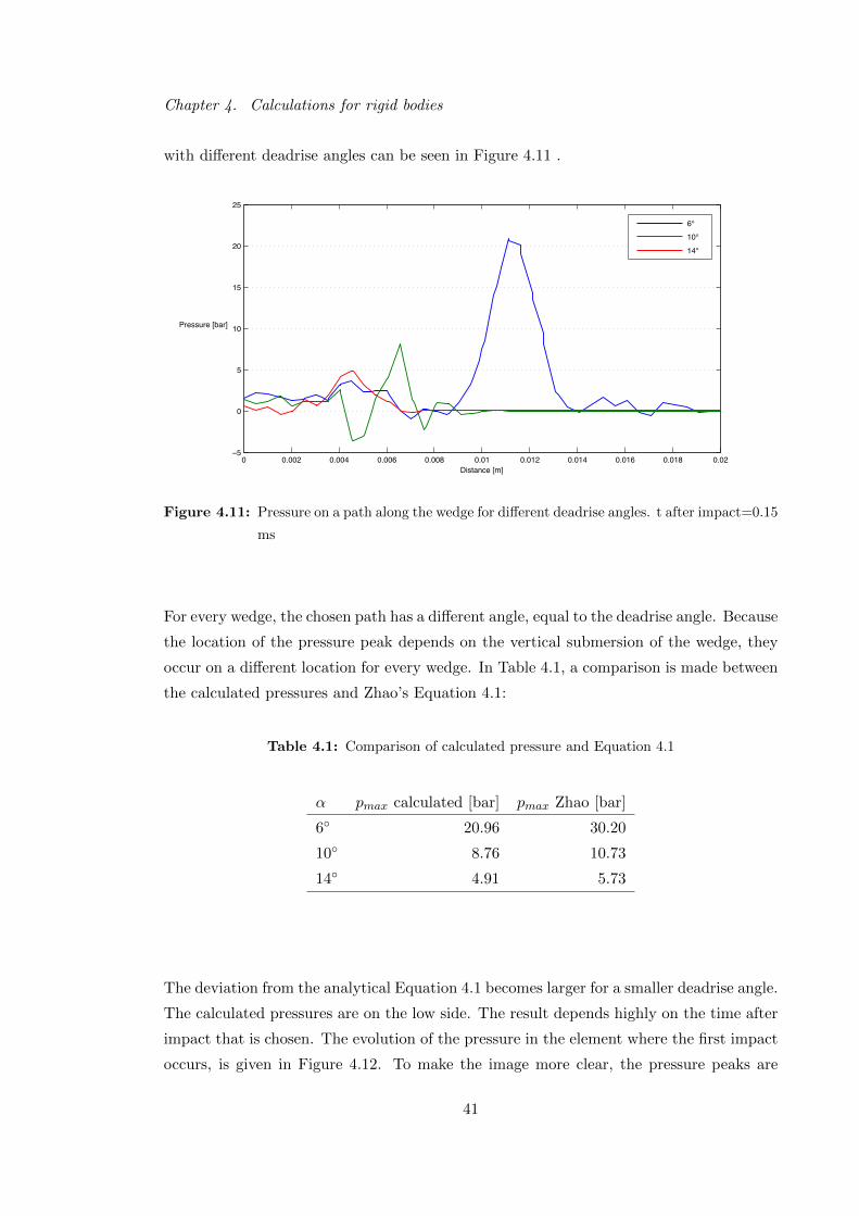
Chapter 4. Calculations for rigid bodies
with different deadrise angles can be seen in Figure 4.11 .
0 0.002 0.004 0.006 0.008 0.01 0.012 0.014 0.016 0.018 0.02−5
0
5
10
15
20
25
Distance [m]
Pressure [bar]
6°
10°
14°
Figure 4.11: Pressure on a path along the wedge for different deadrise angles. t after impact=0.15
ms
For every wedge, the chosen path has a different angle, equal to the deadrise angle. Because
the location of the pressure peak depends on the vertical submersion of the wedge, they
occur on a different location for every wedge. In Table 4.1, a comparison is made between
the calculated pressures and Zhao’s Equation 4.1:
Table 4.1: Comparison of calculated pressure and Equation 4.1
α pmax calculated [bar] pmax Zhao [bar]
6 20.96 30.20
10 8.76 10.73
14 4.91 5.73
The deviation from the analytical Equation 4.1 becomes larger for a smaller deadrise angle.
The calculated pressures are on the low side. The result depends highly on the time after
impact that is chosen. The evolution of the pressure in the element where the first impact
occurs, is given in Figure 4.12. To make the image more clear, the pressure peaks are
41

Chapter 4. Calculations for rigid bodies
given a certain offset along the x-axis, and the moments of first impact are indicated. The
maximum pressures obtained here differ from the maximum pressures calculated along the
wedge. For α = 10 and α = 14, they are higher than the values predicted by Equation
4.1. For α = 6, however, it is much lower. Also, extremely large negative pressures
occur.
1.5 2 2.5 3 3.5 4 4.5 5 5.5 6
x 10−4
−35
−30
−25
−20
−15
−10
−5
0
5
10
15
20
Time [s]
Pressure [bar]
6°
10°
14°
Figure 4.12: Pressure evolution in element where first impact occurs for different deadrise angles
To illustrate that the pressures vary highly from element to element and from frame to
frame, the pressure history in an element is shown in Figure 4.13; the element is located
along the wedge, 3mm horizontal from the axis of symmetry. The pressure reaches 14.90
bar, when a maximum pressure of 5.73 bar is expected.
42

Chapter 4. Calculations for rigid bodies
4 5 6 7 8 9
x 10−4
−10
−5
0
5
10
15
Time [s]
Pressure [bar]
Figure 4.13: Pressure history in element located 3 mm from axis of symmetry. α = 14
Influence of the implementation of air
A more realistic approach can be obtained by implementing a layer of air above the water
surface. However, for a rigid object the results should not differ much from the results
without air because cushioning cannot take place, and drag forces for the velocity used
are very small compared to gravitational force. First, the vertical velocity between the
models with and without air is compared (Figure 4.14). The start of the second step in the
analysis, where the initial velocity is disabled and the wedge moves only under the influence
of gravity, is indicated. When air is not implemented, the wedge accelerates due to gravity,
but with air, the wedge immediatly slows down, which can be explained as follows: In
Abaqus™ it is not possible to model a slamming event with two different eulerian domains,
one for the water and one for the air, because they cannot interact. In order to model the
interaction between the water and the object, a rough contact interaction is applied for
the whole eulerian domain, so the same contact interaction applies for the contact between
air and the impacting object. Because this interaction is rough, the wedge slows down
more than is expected physically, leading to a difference in velocity of the wedge between
the two models. A smaller maximum pressure in the case where air is implemented is
expected. However, because the difference in velocity is small, the maximum pressures
should not differ that much.
43

Chapter 4. Calculations for rigid bodies
0 1 2 3 4 5 6 7x 10⁻⁴
5.14
5.15
5.16
5.17
5.18
5.19
5.2
5.21
Time [s]
Vertical velocity [m/s]
airno air
Figure 4.14: Vertical velocity for model with and without air. α = 10
The pressure on a path along the wedge is given in Figure 4.15. A maximum pressure of
8.50 bar is obtained, which is indeed slightly smaller than when air is not implemented.
The second peak pressure (8.50 bar) is higher than the first peak pressure (8.37). Altough
Figure 4.14 clearly shows that the wedge slows down in time, the pressure increases in
time. However, this increase is very small and can be considered insignificant.
44

Chapter 4. Calculations for rigid bodies
0 0.005 0.01 0.015 0.02−1
0
1
2
3
4
5
6
7
8
9
Distance [m]
Pressure [bar]
t = 0.235 ms
t = 0.400 ms
Figure 4.15: Pressure along wedge for two different timesteps. α = 10
The squeeze-velocity of the air, which is the horizontal velocity, is shown in Figure 4.16,
and is much higher than the vertical velocity in this case. A maximum value of 75.5 m/s
is obtained, but the air mach-number does not exceed M = 0.3. As such, this clearly
justifies the modelling of air as in incompressible gas, since up to mach-numbers of 0.3,
the divergence of the governing equations between an incompressible and a compressible
fluid is only about 1% [29].
45

Chapter 4. Calculations for rigid bodies
(a) t after impact = 0 ms
(b) t after impact = 0.13 ms
Figure 4.16: Horizontal velocity of air for two different timesteps. α = 10
4.3 Cone
4.3.1 Introduction
The cone is a three-dimensional version of the wedge, rotated around its axis of symmetry.
Steel (ρ = 7800 kg, E = 210GPa, ν = 0.3) is used as material. The conus has a diameter
of 300 mm, and the deadrise angle α is 10. To reduce calculation time, only one fourth
of the cone is modeled. Calculations on one eight of a cone were also performed, but
the results were not accurate in the area around the axis of symmetry, where the brick
elements had a corner of 45. Because a rigid body constraint is applied, linear brick
elements are used to model the cone, in order to reduce calculation time.
The implemented boundary conditions for the cone are as follows:
• Initial velocity (Figure 4.17(a))
46
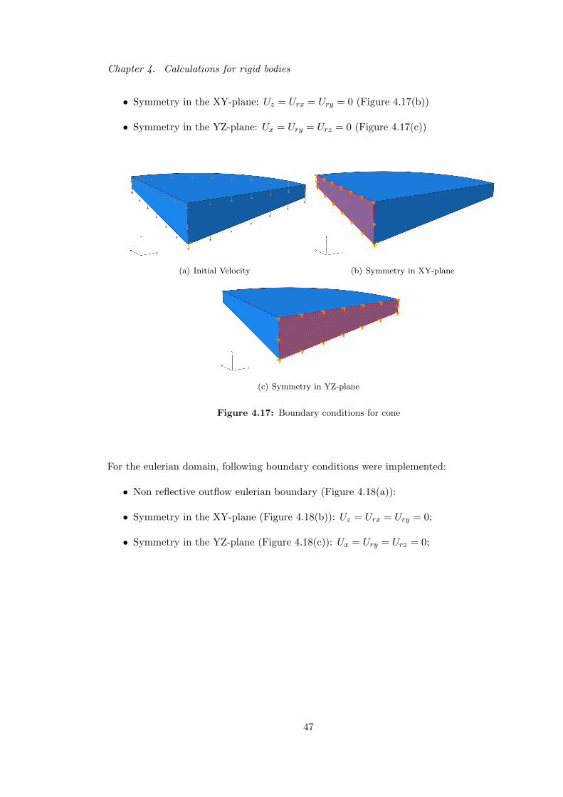
Chapter 4. Calculations for rigid bodies
• Symmetry in the XY-plane: Uz = Urx = Ury = 0 (Figure 4.17(b))
• Symmetry in the YZ-plane: Ux = Ury = Urz = 0 (Figure 4.17(c))
(a) Initial Velocity (b) Symmetry in XY-plane
(c) Symmetry in YZ-plane
Figure 4.17: Boundary conditions for cone
For the eulerian domain, following boundary conditions were implemented:
• Non reflective outflow eulerian boundary (Figure 4.18(a)):
• Symmetry in the XY-plane (Figure 4.18(b)): Uz = Urx = Ury = 0;
• Symmetry in the YZ-plane (Figure 4.18(c)): Ux = Ury = Urz = 0;
47

Chapter 4. Calculations for rigid bodies
(a) Non reflective (b) Symmetry in XY-plane
(c) Symmetry in YZ-plane
Figure 4.18: Boundary conditions for eulerian domain
The explanation of the boundary conditions, both for the cone and the eulerian domain,
is the same as for the wedge. Furthermore, a general view of the model with applied
boundary conditions can be seen in Figure 4.19.
Figure 4.19: General view of the cone model with applied boundary conditions.
48

Chapter 4. Calculations for rigid bodies
4.3.2 Results
Pressure
First, the same impact velocity V = 5.2m/s as for the wedge is used, but to see the
influence of the impact velocity, a simulation with V = 2.6m/s is also performed. The
influence of the impact velocity is very clear from Figure 4.20, where the pressure is shown
for the element where the first contact between the cone and the water surface takes
place. Since pmax ∼ V 2 (see Equation 4.1), the maximum pressure should be 4 times
higher when the impact velocity is doubled. For V = 5.2m/s, a maximum pressure of
11.1 bar is reached, resulting in a pressure coefficient Cp = 82.10. For V = 2.6m/s,
the maximum pressure is 3.69 bar, with a pressure coefficient Cp = 109.17. Altough the
impact pressure is much lower when the impact speed is halved, it is still higher than
expected.
1.5 2 2.5 3 3.5 4 4.5 5 5.5 6 6.5
x 10−4
−15
−10
−5
0
5
10
15
Time [s]
Pressure [bar]
v = 5.2 m/sv = 2.6 m/s
Figure 4.20: Pressure evolution in element were first impact takes place for two different impact
velocities. α = 10
The pressure on a path along the cone is visualised in Figure 4.21, where the path is
defined parallel to the cone, just as for the wedge, and has an angle of 45with respect
to the XY-plane. The time after impact is 0.165 ms. Again, there is clearly a difference
when the impact velocities are different. For V = 5.2m/s, the maximum pressure is 10.30
bar, while for V = 2.5m/s, the pressure reaches 3.28 bar.
49

Chapter 4. Calculations for rigid bodies
0 0.002 0.004 0.006 0.008 0.01 0.012 0.014 0.016 0.018 0.02−1
0
1
2
3
4
5
6
Distance [m]
Pressure [bar]
v = 5.2 m/sv = 2.6 m/s
Figure 4.21: Pressure on a path along the cone for two different impact speeds. α = 10
The cone is relatively heavy since it is made of steel, and only the first stages of the impact
is studied. This means there is a strong gravitational force on the cone, while only a little
wetted surface is in contact with the water. The upward force on the cone is small. As
a result, the cone does not immediatly slow down when it hits the water. Only when the
wetted surface has become large enough, it slows down. The vertical velocity of the cone
throughout the simulation is shown in Figure 4.22; the point of impact is denoted by the
dotted line. However, the variation in velocity is rather small. The calculation can be
considered as performed with a constant velocity.
50

Chapter 4. Calculations for rigid bodies
1 2 3 4 5 6 7
x 10−4
5.195
5.196
5.197
5.198
5.199
5.2
5.201
5.202
5.203
5.204
5.205
Time [s]
Vertical velocity [m/s]
Figure 4.22: Vertical velocity of rigid cone. α = 10
Comparison with experimental results
The calculated results are compared with experimental results obtained by Peseux et al.[2],
where tests on both rigid and deformable cones were performed, and compared with their
own numerical model, which was discussed in chapter 2. In the experimental setup, the
cone is equiped with two pressure sensors. The first one is placed along the cone 40 mm
from the tip, the second one is placed 90 mm from the tip. The location of both sensors can
be seen in Figure 4.23(a). To obtain a constant velocity throughout the experiment, the
velocity is measured at the point of impact with a cable sensor connected to the support,
and is controlled and kept constant from that moment on. The experimental setup can
be seen in Figure 4.23(b).
51

Chapter 4. Calculations for rigid bodies
(a) Location of the pressure sensors (b) Experimental setup
Figure 4.23: Experiments by Peseux et al.[2]
Their results for a rigid cone with impact velocity V = 5.2m/s and deadrise angle α are
shown in Table 4.2. From these results it can be concluded that the pressures calculated
with Abaqus™ are highly conservative, since they almost double the experimental values,
and are 50% larger than the value obtained with the numerical model.
Table 4.2: Experimental and numerical results by Peseux [2]
Experimental [bar] P1 3.9
P2 5.5
Numerical [bar] 7
4.4 Cylinder
4.4.1 Introduction
A series of slamming tests is performed for a rigid cylinder. This is a more difficult object
to perform a calculation on than a wedge. The wedge has a first contact with only one
singular element, after which there is a linear submersion. For the cylinder, this is not the
case. After first contact, a large part of the cylinder surface quickly slams on the water
surface.
The model parameters are chosen as follows:
52

Chapter 4. Calculations for rigid bodies
• cylinder diameter: 300 mm
• thickness: 3 mm
• material: steel (ρ=7800 kg/m3, E=290 GPa, ν=0.3)
• initial velocity: 5 m/s
The cylinder is modelled using shell elements S4R, and a rigid body constraint is applied,
with a reference point in the center of the cylinder. The same type of boundary conditions
as for the wedge are implemented for the cylinder:
• Initial velocity (Figure 4.24(a))
• Symmetry in the XY-plane: Uz = Urx = Ury = 0 (Figure 4.24(b))
• Symmetry in the YZ-plane: Ux = Ury = Urz = 0 (Figure 4.24(c))
(a) Initial velocity (b) Symmetry in XY-plane (c) Symmetry in YZ-plane
Figure 4.24: Boundary conditions for cylinder
The boundary conditions for the eulerian domain are exactly the same as for the eulerian
domain used in the model for the wedge, because the domains are equal. Also, the same
mesh element size is used.
53

Chapter 4. Calculations for rigid bodies
4.4.2 Results
The pressure in the water on a circular path along the cylinder can be seen in Figure 4.26,
where the path is defined in the same way as for the wedge, but is now circular (Figure
4.25).
Figure 4.25: Circular path to visualise pressure along cylinder
At first impact, represented by the blue curve, the pressure reaches 45.8 bar. 0.065 ms
after impact, the maximum pressure is even 51.8 bar. Afterwards the pressure decreases,
as is expected because the cylinder slows down. The pressure history for two elements
in time is shown in Figure 4.27. A maximum pressure of 44.2 bar is obtained. There
is stil a lot of noise after the pressure peak has passed. For the element that is located
23 mm away from the axis of symmetry, there is some influence of the flowfield before
the maximum pressure is obtained. The difference in width of the pressure peak between
Figure 4.26 and Figure 4.27 shows that the pressure peak occurs very shortly in time, but
is more spread out in space.
54

Chapter 4. Calculations for rigid bodies
0 0.005 0.01 0.015 0.02 0.025 0.03 0.035−10
0
10
20
30
40
50
60
Distance [m]
Pressure [bar]
t = 0 mst = 0.065 mst = 0.265 ms
Figure 4.26: Pressure on a path along the cylinder for three different timeframes
2 3 4 5 6 7 8
x 10−4
−10
0
10
20
30
40
50
Time [s]
Pressure [bar]
x = 23 mmx = 0 mm
Figure 4.27: Pressure history for two different elements
An overview of the pressure in the water can be seen in Figure 4.28 and 4.29:
Several trends can be seen:
• The maximum pressure occurs at the point were, at that time, impact takes places.
This is the point where the flow eventually overturns to form a jet.
55

Chapter 4. Calculations for rigid bodies
• A strong shock wave with large negative pressures occurs. This is not seen in liter-
ature.
• The value of the maximum pressures vary highly from frame to frame, but eventually
the pressure reaches a smaller value (Figure 4.29(c)) than the initial values. This
shows again that the value of the maximum pressure is dependent of the time frame
that is chosen. The reason for this is that the pressure can become very high in
a single isolated element, due to numerical instabilities, which Figure 4.30 clearly
demonstrates. A maximum pressure of 85.8 bar is reached in that timeframe, which
is much higher than in most of the other timeframes.
56

Chapter 4. Calculations for rigid bodies
(a) first impact
(b) t after impact = 0.005 ms
(c) t after impact = 0.025 ms
Figure 4.28: Evolution of the pressure in the water domain for the impact of a 2D rigid cylinder,
part 1
57

Chapter 4. Calculations for rigid bodies
(a) t after impact = 0.09 ms
(b) t after impact = 0.41 ms
(c) t after impact = 0.5 ms
Figure 4.29: Evolution of the pressure in the water domain for the impact of a 2D rigid cylinder,
part 2
58

Chapter 4. Calculations for rigid bodies
Figure 4.30: Very high pressure in a single element caused by a numerical instability. Non-
averaged values.
Implementation of air
When a layer of air is implemented above the water surface, the following results are
obtained for the pressure along the cylinder on two different timesteps:
0 0.005 0.01 0.015 0.02 0.025 0.03 0.035 0.04−5
0
5
10
15
20
25
Distance [m]
Pressure [bar]
t = 0 mst = 0.3 ms
Figure 4.31: Pressure along cylinder for two different output frames when air is implemented
59

Chapter 4. Calculations for rigid bodies
At first impact, a maximum pressure of 22.3 bar is reached, which is lower than compared
to the results calculated without air; the air damps the impact because the velocity de-
creases rapidly. Due to the shape of the cylinder, this effect is stronger than in the case of
a wedge. Therefore, the maximum pressure is lower, but this is mainly due to the decrease
in velocity and the rough fricition between the cylinder and the air. The pressure peak
also decreases with time, as is expected. However, when looking at the pressure in time
for a single element (Figure 4.32), it can be seen that the pressure can reach very high
values in a single element, and that there is a lot of fluctuation in the pressure. When
extracting the results along a path, the pressures are averaged along the surrounding ele-
ments. However, for the evolution of the pressure in a single element, this is not the case,
hence the difference in pressure between Figure 4.31 and Figure 4.32. This proves again,
that very high pressure occur in a single element, and that the results must be interpreted
with caution.
2 3 4 5 6 7 8 9 10
x 10−4
−10
−5
0
5
10
15
20
25
30
35
Time [s]
Pressure [bar]
x = 0 mmx = 23 mm
Figure 4.32: Pressure history in time for two different elements when air is implemented.
Comparison with experimental results
In order to assess the correctness and accuracy of the calculations, they are compared
with the experiment results obtained by Lin and Shieh [4], who performed tests on acrylic
cylinders with diameter 0.2 m and 0.3 m. Their results are given in dimensionless form
in Figure 4.33. A comparison with Wagners theory is made, and it can be seen that the
deviation is larger for smaller angles.
60

Chapter 4. Calculations for rigid bodies
Figure 4.33: Results of Lin and Shieh [4]. Dimensionless pressure
A summary of the results calculated with Abaqus™can be found in Table 4.3:
Table 4.3: Maximum pressure coeffecient for different locations on the cylinder
sin(θ) = x/R Cpmax
Without air 0 414.4
0.1533 403.6
With air 0 280.0
0.1533 228.3
The actual velocities were used to calculate the maximum pressure coefficient. Altough it
can not be stated that the experimental results are the real maximum pressure coefficient,
it is clear that the pressures that are calculated using Abaqus™ are very high. For x/R = 0,
Lin and Shieh obtain a Cpmax of 75. This is more than 5 times smaller than the calculations
done without air, and more than 3 times smaller than the calculations with air.
61

Chapter 4. Calculations for rigid bodies
Comparison with numerical model
A comparison is made with the numerical results of Battistin and Iafrati [3] (see Figure
4.34) who developed a numerical model for symmetric and axisymmetric bodies, in which
the effects of gravity and surface tension are neglected. Moreover, the water is considered
incompressible, and air is not implemented. Their results are also compared with the
asymptotic solution by Zhao [1]. The results are given in dimensionless form for different
values of z/R, where z is the penetration depth, and R is the radius of the cylinder. The
dimensionless form of the arc length on the cilinder, y/R, is found on the x-axis, where y
denotes the arc lenght. The pressure is written in dimensionless form using the pressure
coefficient Cp, in function of the dimensionless arc length.
In the initial stage of the water impact, their results are in good agreement with the asymp-
totic theory. For larger values of y/R, the difference increases, because the asymptotic
theory is not accurate for larger deadrise angles.
Figure 4.34: Results by Battistin and Iafrati [3]. Left: Free surface for cylinder and sphere
for z = 0.01 and z = 0.05. Right: Pressure coefficient Cp corresponding to the
penetration depth on the left.
As can be seen in Figure 4.35 the shape of the curve corresponds quite well with the nu-
merical results by Battistin and Iafrati. The value of the pressure coefficient Cp, however,
is much higher than in Figure 4.34, for both values of z/R.
62

Chapter 4. Calculations for rigid bodies
0 0.05 0.1 0.15 0.2 0.25 0.3 0.35 0.4 0.45 0.5−20
0
20
40
60
80
100
120
140
160
180
y/R
Cp
z/R = 0.01z/R = 0.05
Figure 4.35: Dimensionless pressure for different dimensionless penetration depths z/R
Formation of the jet
Lin and Shieh [4] used high speed cameras to capture the appearance of the jet and spray
that forms when the cylinder slams on the water. A comparison is made between their
experimental results, and the calculations performed with Abaqus™. The diameter D of
the cylinder is 100 mm, and the initial velocity is 1 m/s. Their experiment is shown in
Figure 4.36, in which can be seen that in the first stage of impact, after the pressure
has occured, droplets form. Next, the water rises up along the cylinder, and eventually
separates for the cylinder. This happens in a timeframe of about 0.1 s. The water surface
calculated with Abaqus™ can be seen in Figure 4.37. Figure 4.37(b) shows that the amount
of droplets that is formed is small when compared with the experimental results. This
can be atributed to the fact that the eulerian elements have a width and length of 0.5
mm. Droplets that are much smaller than these dimensions are not formed. At 0.006 s
after impact, the flow starts to overturn to form a jet. The splashing starts somewhat
later than in the experimental setup. Except for the amount of droplets, the free surfaces
match quiet well. The elevation of the free surface in the outer region is the same for both
the experiments and the calculations. The direction of the spray also corresponds with
the experiments.
63

Chapter 4. Calculations for rigid bodies
(a) t = 0 − 0.0057s (pres-
sure occurs)
(b) t = 0.0057 − 0.0114s
(splashing)
(c) t = 0.0114 − 0.017s
(splashing)
(d) t = 0.017 − 0.0288s
(splashing)
(e) t = 0.0228 − 0.0285s
(rising up)
(f) t = 0.0285 − 0.0342s
(rising up)
(g) t = 0.0341 − 0.0398s
(rising up)
(h) t = 0.0398 − 0.0455s
(separation)
(i) t = 0.0512 − 0.0.0569s
(separation)
(j) t = 0.0626 − 0.0683s
(separation)
(k) t = 0.0740 − 0.0796s
(separation)
(l) t = 0.0853 − 0.0910s
(separation)
Figure 4.36: Visualisation of the flow field for a cylinder slamming on a flat water surface obtained
by Lin and Shieh[4]. D = 100mm and v = 1m/s.
64

Chapter 4. Calculations for rigid bodies
(a) t = 0.003s (pressure oc-
curs)
(b) t = 0.006s (rising up) (c) t = 0.015s (splashing)
(d) t = 0.02s (rising up) (e) t = 0.025s (rising up) (f) t = 0.03s (rising up)
(g) t = 0.035s (separation) (h) t = 0.045s (separation) (i) t = 0.06s (separation)
(j) t = 0.065s (separation) (k) t = 0.08s (separation) (l) t = 0.095s (separation)
Figure 4.37: Volume fractions at different timesteps for an impacting cilinder calculated with
Abaqus™65

Chapter 4. Calculations for rigid bodies
Conclusion
4.5 Sphere
To see the influence of using symmetry in the models, a slamming test was performed on a
sphere, without the use of symmetry, in which the sphere is made of steel (ρ=7800 kg/m3,
E = 210GPa, ν = 0.3), with a thickness of 3 mm. The impact velocity V is 5 m/s .
Figure 4.38: Overview of model with boundary conditions
First, the results are made dimensionless to compare with the results of Battistin and
Iafrati [3] seen in Figure 4.34. The pressure coefficient Cp is given in function of the
dimensionless arc length y/R in Figure 4.39. Due to three-dimensional effects in case of
the sphere, the wetted portion of the body is smaller. This results in a lower pressure
when compared to the cylinder. A maximum pressure coefficient Cp of 140 is obtained
(Figure 4.39), for z = 0.01, while Battistin and Iafrati obtain a maximum value of 80.
The dimensionless pressure calculated here is indeed lower than for the cylinder, but is
still much higher than the values found in literature.
66
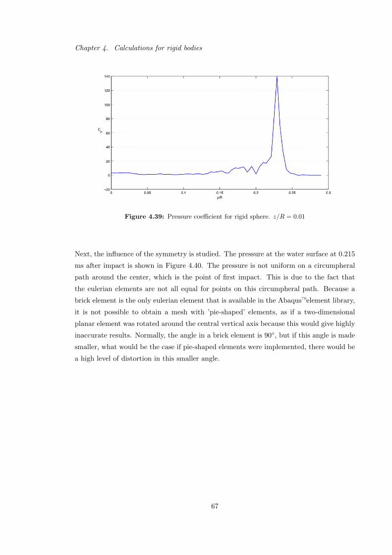
Chapter 4. Calculations for rigid bodies
Figure 4.39: Pressure coefficient for rigid sphere. z/R = 0.01
Next, the influence of the symmetry is studied. The pressure at the water surface at 0.215
ms after impact is shown in Figure 4.40. The pressure is not uniform on a circumpheral
path around the center, which is the point of first impact. This is due to the fact that
the eulerian elements are not all equal for points on this circumpheral path. Because a
brick element is the only eulerian element that is available in the Abaqus™element library,
it is not possible to obtain a mesh with ’pie-shaped’ elements, as if a two-dimensional
planar element was rotated around the central vertical axis because this would give highly
inaccurate results. Normally, the angle in a brick element is 90, but if this angle is made
smaller, what would be the case if pie-shaped elements were implemented, there would be
a high level of distortion in this smaller angle.
67

Chapter 4. Calculations for rigid bodies
Figure 4.40: Water surface for impact of rigid sphere. Time after impact=0.215 ms
4.6 Conclusion
For the wedge, the obtained maximum pressures correspond quite well with Zhao’s ex-
pression for the maximum pressure. However, due to numerical instabilities, the pressure
can reach abnormally high values in some elements. A lot of noise is present in the pres-
sure history plots, and because large negative pressures occur, the flow pattern does not
correspond with patterns found in literature. The influence of the deadrise angle α can
clearly be seen: the pressure decreases when α increases, as expected, but the deviation
from Equation 4.1 increases when α decreases.
The results for the cone were compared with numerical and experimental results, from
which it appears that the calculated pressures are too high. The influence of the impact
velocity V can clearly be seen: the pressure is lower when V decreases.
For the cylinder, the pressures calculated with Abaqus™ are much higher than the
values found in literature, and large negative pressures occur. Moreover, in some elements
the pressure can also become very high due to numerical instabilities. However, the
formation of the jet and the water surface elevation in the Abaqus™simulation match
quite well with experimental results.
Somewhat lower pressures are obtained for both the cylinder and the wedge, when air
is implemented, altough the difference should not be great for rigid bodies. The lower
pressure can be explained by the fact that a rough interaction between the air and the
68

Chapter 4. Calculations for rigid bodies
falling object is applied, meaning that the object immediately slows down, with a lower
pressure as a result. From this, it can be concluded that the drag caused by the air is too
large, and that the air has a rather stiff behaviour.
In general, it can also be noted that the resulting pressure depends highly on the
element and timestep chosen.
69

Chapter 5
Calculations on deformable bodies
5.1 Introduction
In this chapter, Fluid-Structure Interaction (FSI) calculations are performed. The local
pressure peak will deform the impacting object, which in return the will influence the
pressure distribution. This is a more realistic approach of real life slamming events. Dif-
ferent testcases are studied and the influence of the material properties are examined for
a cylinder, by implementing both steel and composite materials. In all cases, the same
boundary conditions as for the rigid bodies are implemented.
5.2 Wedge
5.2.1 Introduction
The wedge is made of steel plate with thickness 1 mm, to be able to study the influence of
the deformation of te structure, because a massive steel wedge would not deform enough
in the first stage of the impact. In Abaqus™, the wedge is modelled as a solid, and Figure
5.1 shows the model together with the applied boundary conditions, which are the same
as for the rigid wedge described in Paragraph 4.2.1, but without a rigid body constraint.
As for the rigid wedge, the impact velocity is 5.2 m/s. Because the thickness is small,
quadratic tetrahedral elements (C3D10M) were used to mesh the wedge [27], with a size
of 0.5 mm for the smallest element edges.
70

Chapter 5. Calculations on deformable bodies
Figure 5.1: Domain with boundary conditions for calculation on deformable wedge
5.2.2 Results
Deformation
The deformation of the wedge througout the analysis is shown in Figure 5.2, with a scaling
factor 20. From Figure 5.2(c) it appears that the left bottom part of the wedge is not the
lowest point, which is not the case, but a result of the use of a scaling factor to make the
deformations more visible. The maximal occuring Von Mises stress σv is 177.7 MPa, and
is derived from the stress tensor using Equation 5.1. If the Von Mises stress is higher than
the material yield strength, plastic deformation will occur. For typical steels, the yield
stress is 250 MPa, so the wedge will not yield during the analysis.
σv =
√(σ11 − σ22)2 + (σ22 − σ33)2 + (σ33 − σ11)2 + 6σ212 + 6σ223 + 6σ223
2(5.1)
71

Chapter 5. Calculations on deformable bodies
(a) t after impact=0.25 ms
(b) t after impact=0.50 ms
(c) t after impact=0.75 ms
(d) t after impact=1.00 ms
Figure 5.2: Deformation of a steel wedge. α = 10
Pressure
The pressure is expected to be somewhat lower due to deformation [2]. Figure 5.3 shows
the pressure on a path along the wedge at two different times after impact. For the first
timestep, a maximum pressure of 8.64 bar is obtained, while for the second output frame
the maximum pressure is 8.62 bar. This is indeed lower than the maximum pressures
obtained for a rigid wedge. However, sometimes the pressure reaches an extremely high
value in a single element due to a numerical instability, as can be seen in Figure 5.4.
72

Chapter 5. Calculations on deformable bodies
0 0.005 0.01 0.015 0.02 0.025−6
−4
−2
0
2
4
6
8
10
Distance [m]
Pressure [bar]
t = 0.3 mst = 0.47 ms
Figure 5.3: Pressure on a path along the wedge for two different output frames. α = 10
Figure 5.4: Numerical instability for the impact of a deformable wedge, 0.025 ms after impact.
α = 10
For a wedge with deadrise angle α = 10, the implementation of air should not cause a
big difference in pressure, because the deadrise angle is too large to see a large amount of
cushioning, and the deformations are relatively small. However, as seen for rigid bodies,
the air does have an influence on the velocity of the wedge, due to the rough friction
73

Chapter 5. Calculations on deformable bodies
between the wedge and the air. Here, this is also the case, as can be seen in Figure
5.5. Moreover, it must be noted that the diffference in velocity is larger than for rigid
wedges due to deformation (see also Figure 4.14), so the pressure should be lower when
air is implemented. In Figure 5.6 the pressure on a path along the wedge is shown, for
t after impact = 0.47 ms, just as in Figure 5.3. With air, the maximum pressure is 5.27
bar, against 8.62 bar when air is not implemented. The difference between the maximum
pressures with and without air is larger when deformation is taken into account, meaning
that the deformation does not allow the air to squeeze as easily as for rigid bodies. This
shows that the air is modelled rather stiff.
0 0.2 0.4 0.6 0.8 1 1.2 1.4
x 10−3
1
1.5
2
2.5
3
3.5
4
4.5
5
5.5
Time [s]
Vertical velocity [m/s]
No airAir
Figure 5.5: Vertical velocity for a deformable wedge
74

Chapter 5. Calculations on deformable bodies
0 0.005 0.01 0.015 0.02 0.025 0.03−1
0
1
2
3
4
5
6
Distance [m]
Pressure [bar]
Figure 5.6: Pressure on path along wedge when air is implemented. t after impact = 0.47 ms
5.3 Cone
5.3.1 Introduction
The cone is made of steel plate with thickness=1 mm for the same reason as for the
wedge, and the domain and boundary conditions can be seen in Figure 5.7. The boundary
conditions are the same as for the rigid cone described in Paragraph 4.3.1, and the same
element type as for the wedge is used (see Paragraph 5.2.1). To be able to compare the
obtained results with the work of Peseux et al. [2], the impact velocity V is set to 2.5
m/s.
75

Chapter 5. Calculations on deformable bodies
Figure 5.7: Domain with boundary conditions for calculation on deformable cone
5.3.2 Results
Pressure
Figure 5.8 shows the pressure evolution in the element where the first impact takes place
for three different values of the deadrise angle α, where the dotted line represents the
moment of impact. To make the image more orderly, the pressure curves were given a
certain offset along the x-axis. The resulting maximum pressures are given in Table 5.1,
where they are compared with experimental and numerical results obtained by Peseux
[2]. For their experiments, they also used a deformable cone with thickness=1 mm. The
maximum pressures obtained with Abaqus™ are very high compared with these results.
However, it must be noted that the highest pressure which can be seen in Figure 5.8 are
not appearing at first impact, but somewhat later, and are reached in a single timestep
only. Furthermore, for α = 6, there are two peaks visible, which could be caused by a
numerical instability. When looking at the pressures at first impact, they are lower and
correspond more with the results of Peseux, but are still on the high side.
76

Chapter 5. Calculations on deformable bodies
0 1 2 3 4 5 6 7
x 10−4
−8
−6
−4
−2
0
2
4
6
8
Time [s]
Pressure [bar]
! = 6°! = 10°! = 14°
Figure 5.8: Pressure evolution in element where first impact of a deformable cone occurs, for
different values of α
Table 5.1: Comparison of results by Peseux [2] and calculated results for deformable cone
α Peseux Experimental [bar] Peseux Numerical [bar] Abaqus™[bar]
6 1.4 2.2 6.67
10 1.2 1.3 4.83
14 0.6 0.6 3.66
77

Chapter 5. Calculations on deformable bodies
5.4 Cylinder
5.4.1 Introduction
The same cylinder is used as in Chapter 4, but is now modelled as a deformable solid.
Calculations with a deformable shell (element type S4R [27], element size 0.5 mm) were
also performed, but no significant difference in the results arose. The impact velocity of
the cylinder is 5 m/s, the outer diameter D=300 mm, and only half of the cylinder is
modelled, using symmetry boundary conditions. 4 layers of linear brick elements with
reduced integration (C3D8R) were used to model the cylinder [27]. The shortest edge of
the element is 0.5 mm.
5.4.2 Results
Deformation
First, the deformation of the cylinder is studied. The cylinder is made out of steel,
modelled as a linear elastic material (ρ = 7800 kg/m3, E = 210GPa, ν = 0.3). The
deformation througout the analysis can be seen in Figure 5.9. Note that the deformation
is scaled with factor 20 to make it more visible. As expected, the deformation is mostly
concentrated in the area where slamming takes place, because only a small part of the
cylinder experiences the opposing force of the water.
78
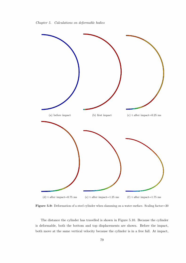
Chapter 5. Calculations on deformable bodies
(a) before impact (b) first impact (c) t after impact=0.25 ms
(d) t after impact=0.75 ms (e) t after impact=1.25 ms (f) t after impact=1.75 ms
Figure 5.9: Deformation of a steel cylinder when slamming on a water surface. Scaling factor=20
The distance the cylinder has travelled is shown in Figure 5.10. Because the cylinder
is deformable, both the bottom and top displacements are shown. Before the impact,
both move at the same vertical velocity because the cylinder is in a free fall. At impact,
79

Chapter 5. Calculations on deformable bodies
the bottom is slowed down first, and the top part still moves further down. The relative
deviation of the diameter (DOD) is shown in Figure 5.11, and is calculated with Equation
5.2. When the impact occurs, the diameter changes in a linear way. At the end of the
calculation, 2.2 ms after impact, the relative deformation is 1.29%.
DOD =original diameter − deformed vertical diameter
original diameter· 100 (5.2)
0 0.5 1 1.5 2 2.5
x 10−3
0
0.002
0.004
0.006
0.008
0.01
0.012
Time [s]
Distance [m]
Top
Bottom
Figure 5.10: Displacement for both the top and the bottom of the cylinder
80

Chapter 5. Calculations on deformable bodies
0 0.5 1 1.5 2 2.5
x 10−3
0
0.2
0.4
0.6
0.8
1
1.2
1.4
Time [s]
DOD [%]
Figure 5.11: Procentual deviation of the original diameter for an impacting cylinder
Pressure
For the pressures, a comparison is made with the work of Battistian and Iafrati [3], of
which the results can be seen in Figure 4.34. The dimensionless pressures obtained with
Abaqus™ are shown in Figure 5.12.
0 0.05 0.1 0.15 0.2 0.25 0.3 0.35 0.4 0.45 0.5−40
−20
0
20
40
60
80
100
120
140
160
y/R
Cp
z/R = 0.01z/R = 0.05
Figure 5.12: Dimensionless pressure for deformable cylinder
81

Chapter 5. Calculations on deformable bodies
For z/R=0.01, a maximum Cp of 141.51 is obtained, which is rather high, but still lower
than for a rigid cylinder. The explanation for this can be found when looking at the vertical
velocity of the cylinder (Figure 5.13) and the actual pressure (Figure 5.14); to calculate
Cp, the velocity of the bottom of the cyilinder was used. As can be seen in the velocity
plot (Figure 5.13), the velocity drops suddenly at impact due to the deformation of the
cylinder, resulting in v = 3.67m/s for z/R = 0.01. This velocity is lower when compared
to the velocity of the rigid cylinder for the same submersion, and as a result the pressure
is much lower after the first impact. When looking at the actual pressure (Figure 5.14), it
can be seen that the actual pressure is indeed lower than in the case of a rigid impact. For
both values of the dimensionless submersion (z/R = 0.01 and z/R = 0.05, Figure 5.12),
the shape of the curve does not correspond as wel with the results in Figure 4.34. There
is a lot of scatter in the pressure, and two pressure peaks are visible. For z/R = 0.05, the
high value of Cp can be explained by the same considerations as for z/R = 0.01, and it
can be concluded that the maximum pressure is lower than for a rigid cylinder, but still
are very conservative, just as for rigid bodies.
0 0.5 1 1.5 2 2.5
x 10−3
2.5
3
3.5
4
4.5
5
5.5
Time [s]
Vertical velocity [m/s]
Figure 5.13: Vertical velocity for deformable cylinder
82

Chapter 5. Calculations on deformable bodies
0 0.005 0.01 0.015 0.02 0.025 0.03 0.035 0.04 0.045 0.05−2
0
2
4
6
8
10
Distance [m]
Pressure [bar]
Figure 5.14: Pressure on a path along a deformable cylinder for z/R = 0.01.
t after impact=0.37 ms
Calculations with air are also performed, with maximum pressures that are somewhat
lower than the pressures obtained with air, but as shown in Chapter 4, this is due to the
lower velocity resulting from the rough interaction between the air and the cylinder. Still,
the pressures are in the same order of magnitute as without air, and are still higher than
the results found in literature.
5.4.3 Composite cylinder
Modelling of the composite lay-up
The point absorbers that will be used in the SEEWEC-project are made out of a composite
material. For that reason, a slamming test is performed on a cilinder made of this material.
The lay-up scheme of the composite (Table 5.3) is the same as used in experimental tests
by Baro and Dervaux [30], performed at the departement of Mechanics of Materials and
Structures. A cylinder with diameter D = 300mm was used in the experiments. The
shell is composed out of 3 layers, and is 3 mm thick in total. The bottom layer is a mat of
short glass fibres, and can be considered isotropic. The next two layers are made of cross
windings of continuous glass fibre, wound under an angle of 70with respect to the the
axis of the cylinder. The mass of the used glass fibre per unit length is 600 TEX, where
1 TEX= 10−6 kg/m. The density of the material ρ = 1900 kg/m3. The properties of the
83

Chapter 5. Calculations on deformable bodies
fibre are given in Table 5.2.
Table 5.2: Properties of glass fibre
E1 Elastic modulus parallel to the fibre direction 25.770 GPa
E2 Elastic modulus perpendicular to the fibre direction 6.2519 GPa
ν12 Poisson ratio 0.38
G12 Shear modulus 4.2 GPa
G13 Shear modulus 4.2 GPa
G23 Shear modulus 2.5 GPa
In Abaqus™, this material is modeled as a linear elastic lamina. Only planar stresses are
considered (σ33 = 0). The shear moduli G13 and G23 are required however because they
may be needed for modeling transverse shear deformation in the shell. The poisson ratio
ν21 is simply determined as (E2/E1)ν12. The material properties for the isotropic fibre
mat are not known, but are attributed to the cylinder as a whole. Because the windings
are crossed, each layer has to be defined twice in Abaqus™, under symmetrical angles. As
can be seen in Figure 5.15, a local cylindrical coordinate system was introduced to define
the material orientations, and eventually the lay-up scheme is given in Table 5.3.
Table 5.3: Modelling of composite lay-up
layer thickness [m] material orientation
1 0.0006 0
2 0.0006 20
3 0.0006 -20
4 0.0006 20
5 0.0006 -20
84

Chapter 5. Calculations on deformable bodies
(a) Layer 1 (b) Layer 2 (c) Layer 3 (d) Layer 4 (e) Layer 5
Figure 5.15: Lay-up scheme with fibre directions in local coordinate system
5.4.4 Results
Deformation
The impact velocity V is 5 m/s, just as for the steel cylinder. Figure 5.17 shows the
deformations, with scaling factor 20 for the composite part. Due to the difference in
stiffness of both materials (represented by the elastic modulus E), the deformation is more
pronounced for the composite cylinder. The use of a scaling factor is necessary to display
the deformations, because otherwise the deformations would not be notable. However,
from Figure 5.17 it appears that the most left bottom point is not the lowest point on the
cilinder, which would not be a deformation that is expected physically. When looking at
the deformation without the scaling factor, it is clear that this is not the case, and the
shape of the cylinder after impact is elliptical. The relative deviation of the diameter is
shown in Figure 5.16, where at the end of the simulation it is 2.05%, which is higher than
for the steel cylinder.
85

Chapter 5. Calculations on deformable bodies
0 0.5 1 1.5 2 2.5
x 10−3
0
0.5
1
1.5
2
2.5
Time [s]
DOD [%]
Figure 5.16: Relative deviation of the diameter for a composite cylinder
86

Chapter 5. Calculations on deformable bodies
(a) before impact (b) first impact (c) t after impact=0.25 ms
(d) t after impact=0.75 ms (e) t after impact=1.25 ms (f) t after impact=1.75 ms
Figure 5.17: Deformation of composity cylinder when slamming on a water surface. Scaling
factor=20
87

Chapter 5. Calculations on deformable bodies
Pressure
Figure 5.18 shows Cp for different values of the dimensionless arc length y/R. The max-
imum pressure coefficient Cp is 411.48, which is very high, but the shape of the curve
resembles quite well with the results by Battistin and Iafrati [3] (Figure 4.34). The expla-
nation for this result is the same as in previous for the steel cylinder: when the dimension-
less submersion is z/R = 0.01, the vertical velocity v is only 1.83 m/s, while the actual
pressure is 6.89 bar. Due to the higher level of deformation, this velocity is lower than for
the steel cylinder. This is the cause of the high pressure coefficient (Cp ∼ 1/v2), rather
than a high value for the maximum pressure itself.
0 0.05 0.1 0.15 0.2 0.25 0.3 0.35−50
0
50
100
150
200
250
300
350
400
450
y/R
Cp
Figure 5.18: Dimensionless pressure for the impact of a composite cylinder. z/R = 0.01
Failure of the material
To determine if the material will fail under impact, the Tsai-Wu failure criterion, which
is a stress based failure criterion, is implemented. A combination of stresses in different
directions may not exceed 1 in order no to fail. The expression for the Tsai-Wu criterion is
shown in Equation 5.3, and can be interpreted as a surface in three dimensions around the
origin defined by σ11, σ22 and σ12. When a certain stress state σ11, σ22, σ12 is outside of
this surface, failure occurs.
IF = F1σ11 + F2σ22 + F11σ211 + F22σ
222 + F66σ
212 + 2F12σ11σ22 < 1 (5.3)
F1, F2, F11, F22, F66 and F12 are determined by the following expressions:
88

Chapter 5. Calculations on deformable bodies
F1 =1
Xt+
1
Xc(5.4a)
F2 =1
Yt+
1
Yt(5.4b)
F11 = − 1
XtXc(5.4c)
F22 = − 1
YtYc(5.4d)
F66 =1
S2(5.4e)
F12 =1
2σ2biax
[1−
(1
Xt+
1
Xc+
1
Yt+
1
Yc
)σbiax +
(1
XtXc+
1
YtYc
)σ2biax
](5.4f)
(5.4g)
or
F12 = f√F11F22 (5.4h)
Xt and Yt are the tensile strength limits in the 1- and 2-direction, Xc and Yc are the
compressive stress limits in the 1- and 2-direction and S is the maximum shear tension in
the 1-2 plane. If the equibiaxial stress at failure σbiax is known, Equation 5.4f is used to
calculate the coupling term F12. When it is not known, Equation 5.4h can be used, where
f is a coefficient with values between -1 and 1. However, it is generally accepted that the
influence of F12 can be neglected [31]. In Abaqus™, both σbiax and f are set to zero. The
values of the stress limits used here are found in [30]: Xt and Xc are 600 MPa, Yt and Yc
are 60 MPa, and S is 50 MPa.
The stresses for the top and bottom layer are shown in Figure 5.19 and 5.20, both in the
direction of (σ11) as well as perpendicular to the fibre orientation (σ22). The shear stress
(σ12) for both layers can be seen in Figure 5.21. In order to visualize the stresses, the
cylinder was stretched in the z-direction, with a scaling factor 500. The time after impact
is 2 ms. The top and bottom layer are shown because these are most crucial, since the
cylinder experiences bending. Figure 5.22 shows the values of IF for the Tsai-Wu failure
criterion. The bottom region of the cylinder that is exposed to the slamming force appears
to most crucial, but the value for IF remains well below 1, meaning that failure will not
occur because the stresses are too low to cause any damage.
89

Chapter 5. Calculations on deformable bodies
(a) bottom layer (b) top layer
Figure 5.19: Stress in the fibre direction (σ11) for the bottom and top layer
(a) bottom layer (b) top layer
Figure 5.20: Stress perpendicular to the fibre direction (σ22) for the bottom and top layer
90

Chapter 5. Calculations on deformable bodies
(a) bottom layer (b) top layer
Figure 5.21: Shear stress (σ12) for the bottom and top layer
(a) bottom layer (b) top layer
Figure 5.22: Tsai-Wu failure criterion
5.5 Conclusion
The maximum pressure for a deformable wedge is slighty lower when compared to a rigid
wedge. However, the influence of air is larger altough the deformation is small, which can
91

Chapter 5. Calculations on deformable bodies
be atributed to the fact that the air is modelled too stiff, and that the drag caused by the
air is higher than expected physically.
For the cone, the maximum pressure is higher when compared to experimental results,
but this may be caused by numerical instabilities causing a high pressure in a single
timestep, because the pressure at first impact is lower. However, it is still higher than the
experimental results found in literature.
Both steel and a composite material were used to model the cylinder. In both cases, the
pressure is lower than for rigid bodies, but is still much higher than numerical results found
in literature. The deformation is rather small, but larger for the composite cilinder, caused
by a smaller stiffnes of the material. Moreover, the deformation has a large influence on
the velocity of the cylinder. Both materials, however, will not fail under impact.
92

Chapter 6
Conclusion
In this thesis the slamming of an object, both rigid and deformable, on a flat water surface
was studied using an Euler-Lagrange coupling in Abaqus™. This feature is rather new in
Abaqus™, and it’s performance for slamming simulations was not yet known.
First, a theoretical explanation of the model parameters was given. With only one way
to implement fluids, the number of options that Abaqus™ has to offer to model fluids is
limited. Also, only one element is available in the element library to mesh an eulerian
domain.
Next, the results of the analysis were presented for both rigid and deformable bodies.
Pressures, water flow, deformations and stresses were studied, and compared with results
found in international literature.
The wedge is the most fundamental geometric shape to perform a calculation with. The
results match quite well with results found in literature, but the difference becomes larger
as the deadrise angle decreases. For a cone, the pressures were overestimated in the
calculations. Moreover, a large amount of oscillation is present in the pressure results, and
sometimes the pressure reaches a very high value in a single element, which is probably
caused by a numerical instability. Large negative values of the pressure occur, because
a shockwave is propagated through the fluid, which is not seen in literature. The origin
of this shockfront is located in the point where the object is entering the water at that
moment.
In case of a cylinder, which is more complex because the deadrise angle starts at 0and
eventually becomes larger, the pressures are largely overestimated. This is also seen for a
sphere, altough the pressure here is lower due to threedimensional effects. The influence of
using symmetry is studied, and it can be concluded that symmetry is useful, because it is
not always possible to create mesh made of eulerian brick that is completely symmetrical as
93
Chapter 6. Conclusion
well. The formation of the jet along the cylinder corresponds quite well with experimental
results, but the amount of spray is lower, because very small droplets are not resolved in
the mesh.
The same conclusions can be made for the flowfield when a deformable object slams on the
water, altough the actual pressures are somewhat lower than in the case of rigid objects,
which is physically correct. The deformation was studied for both steel and a composite
material. In both cases, the deformation is rather small, and no damage in the material
occurs.
Interaction between different eulerian domains is not possible in Abaqus™, so when air is
implement, both water and air must be defined in the same eulerian domain. Because the
interaction between the impacting object and the water must be rough, interaction between
air and the object is also rough. As a result, the drag force of the air is overestimated during
free fall, leading to a lower impact velocity and a lower maximum pressure. Moreover, air is
modelled too stiff, which is notable when the impact of a deformable object is considered.
The maximum pressures, however, are still higher than values found in literature.
In general, it can be concluded that the pressures are overestimated, and that the results
are hard to interpret due to the appearance of numerical instabilities in a single element.
94

Bibliography
[1] Zhao, R. and Faltinsen, O.M.: Water entry of two-dimensional bodies. Journal of
Fluid Mechanics, 246:593–612, 1993.
[2] Peseux, B., Gornet, L., and Donguy, B.: Hydrodynamic impact: Numerical and ex-
perimental investigations. Journal of Fluids and Structures, 21(3):277–303, 2005.
[3] Battistin, D. and Iafrati, A.: Hydrodynamic loads during water entry of two-
dimensional and axisymmetric bodies. Journal of Fluids and Structures, 17:643–664,
2003.
[4] Lin, M. C. and Shieh, L. D.: Flow visualization and pressure characteristics of a
cylinder for water impact. Applied Ocean Research, 19:101–112, 1997.
[5] European Communities, Office for Official Publications of the: Energy, let us overcome
our dependence. ISBN 92-894-1349-2, 2002.
[6] Stenius, I.: Finite element modelling of hydroelasticity in hull-water impacts. Master’s
thesis, KTH Centre for Naval Architecture Aeronautical and Vehicle Engineering,
Stockholm, Sweden, 2006.
[7] Stoop, K. and Vermeulen, S.: Numerical simulation of fluid-structure interaction for
hydrodynamic impact. Master’s thesis, Ghent University, 2008.
[8] Von Karman, T.: The impact on seaplane floats during landing. Technical notes,
National Advisory Committee for Aeronautics, 1929.
[9] Seddon, C.M. and Moatamedi, M.: Review of water entry with applications to
aerospace structures. International Journal of Impact Engineering.
[10] Newman, J.N.: Marine Hydrodynamics. MIT Press, London, 1977.
[11] Wagner, H.: Uber stoss und gleitvorgange an der oberflache von flussigkeiten.
Zeitschrift fur Angewandte Mathematik und Mechanik, 12(4):193–215, 1932.
95

Bibliography
[12] Watanabe, S.: Resistance of impact on water surface, part i—cone. Institute of Phys-
ical and Chemical Research, Tokyo, 12:251–267, 1930.
[13] Watanabe, S.: Resistance of impact on water surface, part ii—cone continued. Insti-
tute of Physical and Chemical Research, Tokyo, 14:153–168, 1930.
[14] Mei, X.M., Liu, Y.M., and Yue, D.K.P.: On the water impact of general two-
dimensional sections. Applied Ocean Research, 21(1):1–15, 1999.
[15] Dobrovol’Skaya, Z.N.: On some problems of similarity flow of fluid with a free surface.
Journal of Fluid Mechanics, 36:805–892, 2006.
[16] Pierson: The penetration of a fluid surface by a wedge. Stevens Institute of Technology
Report 381, 1951.
[17] Cointe, R., Fontaine, E., Molin, B., and Scolan, Y.M.: On energy arguments applied
to the hydrodynamic impact force. Journal of Engineering Mathematics, 48:305–319,
2004.
[18] Longuet-Higgings, M.S. and Cokelet, E.D.: The deformation of steep surface waves on
water. i. a numerical method. Proceedings of the Royal Society, London, 350 A:1–26,
1976.
[19] Iafrati, A., Carcaterra, A., Ciappi, E., and Campana, E.F.: Hydroelastic analysis of
a simple oscillator impacting the free surface. Journal of Ship Research, 44:278–289,
2000.
[20] Souli, M. and Zolesio, J.P.: Arbitrary lagrangian-eulerian and free surface methods in
fluid mechanics. Computer methods in applied mechanics and engineering, 191:451–
466, 2001.
[21] Rabier, S. and Medale, M.: Computation of free surface flows with a projection fem in
a moving mesh framework. Computer methods in applied mechanics and engineering,
192:4703–4721, 2003.
[22] Aquelet, N, Souli, M., and Olovsson, L.: Euler–lagrange coupling with damping effects:
Application to slamming problems. Computer methods in applied mechanics and
engineering, 195:110–132, 2006.
[23] Kleefsman, K.M.T., Fekken, G., Veldman, A.E.P., Iwanowski, B., and Buchner, B.:
A volume-of-fluid based simulation method for wave impact problems. Journal of
Computational Physics, 206(1):363–393, 2005.
96

Bibliography
[24] Hirt, C.R. and Nichols, B.D.: Volume of fluid (vof) method for the dynamics of free
boundaries. Journal of Computational Physics, 39:201–225, 1981.
[25] Rider, William J. and Kothe, Douglas B.: Reconstructing volume tracking. Journal of
Computational Physics, 141:112–152, 1998.
[26] Gerrits, J.: Dynamics of liquid-filled spacecraft. Ph.D. Thesis, University of Gronin-
gen, The Netherlands, 2001.
[27] Abaqus™Documentation v6.9-2 EF, 2010.
[28] Versteeg, H.K. and Malalasekera, W.: An introduction to computational fluid dynam-
ics. the finite volume method., 2007.
[29] Dick, E.: Turbomachinery. Lecture notes, Ghent University.
[30] Baro, W. and Derveaux, T.: Design, realisation and testing of a composite point-
absorber for wave energy converters. Master’s thesis, Ghent University, 2007.
[31] Van Paepegem, W. and Degrieck, J.: Calculation of damage-dependent directional
failure indices from the tsai–wu static failure criterion. Composites Science And
Technology, 63:305–310, 2003.
97

List of Figures
1 Overzicht van rekendomein voor wig . . . . . . . . . . . . . . . . . . . . . . ix
2 Dimensieloze druk voor cilinder bij verschillende waarden van z/R . . . . . x
3 Dimensieloze druk voor bol bij z/R = 0.01 . . . . . . . . . . . . . . . . . . . xi
4 Zeer hoge druk in element door numerieke instabiliteit. Niet-uitgemiddelde
waarden. . . . . . . . . . . . . . . . . . . . . . . . . . . . . . . . . . . . . . . xii
5 Druk in element waar eerste impact plaats heeft, voor verschillende waarden
van α . . . . . . . . . . . . . . . . . . . . . . . . . . . . . . . . . . . . . . . xiii
6 Vervorming voor stalen en composiet cilinder. t na impact is 1.25 ms . . . . xv
7 Procentuele afwijking van originele diameter . . . . . . . . . . . . . . . . . . xv
8 Dimensionless pressure for deformable cylinder . . . . . . . . . . . . . . . . xvi
9 Tsai-Wu failure criterion . . . . . . . . . . . . . . . . . . . . . . . . . . . . xvii
1.1 WEC platform concept . . . . . . . . . . . . . . . . . . . . . . . . . . . . . . 2
1.2 Slamming of composite hull during the 2008 Volvo Ocean Race . . . . . . . 3
1.3 Pressure distribution on an impacting wedge [6] . . . . . . . . . . . . . . . . 4
2.1 Definition of the deadrise angle α . . . . . . . . . . . . . . . . . . . . . . . . 6
2.2 Slamming definitions . . . . . . . . . . . . . . . . . . . . . . . . . . . . . . . 8
2.3 Solution for a wedge obtained by Mei for several deadrise angeles. Com-
parison with the similarity solution obtained by Dobrovol’Skaya. . . . . . . 9
2.4 Fluid domain . . . . . . . . . . . . . . . . . . . . . . . . . . . . . . . . . . . 11
2.5 Boundary conditions in computational domain. . . . . . . . . . . . . . . . . 12
2.6 Cut-off jet in computational domain . . . . . . . . . . . . . . . . . . . . . . 12
2.7 Definition of different domains in computational domain . . . . . . . . . . . 13
2.8 Comparison between cone and wig with same deadrise angle of 10at 4
different timesteps. Impact velocity is 6m/s . . . . . . . . . . . . . . . . . . 14
2.9 Air gets trapped in concave cavities when the impacting object deforms.
The air is compressed and the object slows down. . . . . . . . . . . . . . . . 15
2.10 Structural domain . . . . . . . . . . . . . . . . . . . . . . . . . . . . . . . . 15
98

List of Figures
2.11 Contact algorithm . . . . . . . . . . . . . . . . . . . . . . . . . . . . . . . . 18
2.12 Steps taken to calculate Volume Fraction F . . . . . . . . . . . . . . . . . . 19
2.13 Comparison between the SLIC and PLIC surface reconstruction algorithms 20
2.14 Local height function h . . . . . . . . . . . . . . . . . . . . . . . . . . . . . 21
3.1 Drop test with wooden sphere . . . . . . . . . . . . . . . . . . . . . . . . . . 27
4.1 Meshed wedge, deadrise angle = 10 . . . . . . . . . . . . . . . . . . . . . . 32
4.2 Boundary conditions for wedge . . . . . . . . . . . . . . . . . . . . . . . . . 33
4.3 Boundary conditions for eulerian domain . . . . . . . . . . . . . . . . . . . . 34
4.4 Overview of model domain with applied boundary conditions . . . . . . . . 35
4.5 Path for visualisation of the pressure along the wedge . . . . . . . . . . . . 35
4.6 Pressure along wedge with deadrise angle 10for different timesteps . . . . . 36
4.7 Pressure in three different elements with respect to time. Deadrise angle=10 37
4.8 Pressure for t = 0.595 ms after impact. The results are not averaged . . . . 38
4.9 Evolution of pressure part 1 . . . . . . . . . . . . . . . . . . . . . . . . . . . 39
4.10 Evolution of pressure part 2 . . . . . . . . . . . . . . . . . . . . . . . . . . . 40
4.11 Pressure on a path along the wedge for different deadrise angles. t after
impact=0.15 ms . . . . . . . . . . . . . . . . . . . . . . . . . . . . . . . . . 41
4.12 Pressure evolution in element where first impact occurs for different deadrise
angles . . . . . . . . . . . . . . . . . . . . . . . . . . . . . . . . . . . . . . . 42
4.13 Pressure history in element located 3 mm from axis of symmetry. α = 14 . 43
4.14 Vertical velocity for model with and without air. α = 10 . . . . . . . . . . 44
4.15 Pressure along wedge for two different timesteps. α = 10 . . . . . . . . . . 45
4.16 Horizontal velocity of air for two different timesteps. α = 10 . . . . . . . . 46
4.17 Boundary conditions for cone . . . . . . . . . . . . . . . . . . . . . . . . . . 47
4.18 Boundary conditions for eulerian domain . . . . . . . . . . . . . . . . . . . . 48
4.19 General view of the cone model with applied boundary conditions. . . . . . 48
4.20 Pressure evolution in element were first impact takes place for two different
impact velocities. α = 10 . . . . . . . . . . . . . . . . . . . . . . . . . . . . 49
4.21 Pressure on a path along the cone for two different impact speeds. α = 10 50
4.22 Vertical velocity of rigid cone. α = 10 . . . . . . . . . . . . . . . . . . . . 51
4.23 Experiments by Peseux et al.[2] . . . . . . . . . . . . . . . . . . . . . . . . . 52
4.24 Boundary conditions for cylinder . . . . . . . . . . . . . . . . . . . . . . . . 53
4.25 Circular path to visualise pressure along cylinder . . . . . . . . . . . . . . . 54
4.26 Pressure on a path along the cylinder for three different timeframes . . . . . 55
4.27 Pressure history for two different elements . . . . . . . . . . . . . . . . . . . 55
99

List of Figures
4.28 Evolution of the pressure in the water domain for the impact of a 2D rigid
cylinder, part 1 . . . . . . . . . . . . . . . . . . . . . . . . . . . . . . . . . . 57
4.29 Evolution of the pressure in the water domain for the impact of a 2D rigid
cylinder, part 2 . . . . . . . . . . . . . . . . . . . . . . . . . . . . . . . . . . 58
4.30 Very high pressure in a single element caused by a numerical instability.
Non-averaged values. . . . . . . . . . . . . . . . . . . . . . . . . . . . . . . . 59
4.31 Pressure along cylinder for two different output frames when air is imple-
mented . . . . . . . . . . . . . . . . . . . . . . . . . . . . . . . . . . . . . . . 59
4.32 Pressure history in time for two different elements when air is implemented. 60
4.33 Results of Lin and Shieh [4]. Dimensionless pressure . . . . . . . . . . . . . 61
4.34 Results by Battistin and Iafrati [3]. Left: Free surface for cylinder and
sphere for z = 0.01 and z = 0.05. Right: Pressure coefficient Cp corre-
sponding to the penetration depth on the left. . . . . . . . . . . . . . . . . . 62
4.35 Dimensionless pressure for different dimensionless penetration depths z/R . 63
4.36 Visualisation of the flow field for a cylinder slamming on a flat water surface
obtained by Lin and Shieh[4]. D = 100mm and v = 1m/s. . . . . . . . . . 64
4.37 Volume fractions at different timesteps for an impacting cilinder calculated
with Abaqus™ . . . . . . . . . . . . . . . . . . . . . . . . . . . . . . . . . . . 65
4.38 Overview of model with boundary conditions . . . . . . . . . . . . . . . . . 66
4.39 Pressure coefficient for rigid sphere. z/R = 0.01 . . . . . . . . . . . . . . . . 67
4.40 Water surface for impact of rigid sphere. Time after impact=0.215 ms . . . 68
5.1 Domain with boundary conditions for calculation on deformable wedge . . . 71
5.2 Deformation of a steel wedge. α = 10 . . . . . . . . . . . . . . . . . . . . . 72
5.3 Pressure on a path along the wedge for two different output frames. α = 10 73
5.4 Numerical instability for the impact of a deformable wedge, 0.025 ms after
impact. α = 10 . . . . . . . . . . . . . . . . . . . . . . . . . . . . . . . . . 73
5.5 Vertical velocity for a deformable wedge . . . . . . . . . . . . . . . . . . . . 74
5.6 Pressure on path along wedge when air is implemented. t after impact =
0.47 ms . . . . . . . . . . . . . . . . . . . . . . . . . . . . . . . . . . . . . . 75
5.7 Domain with boundary conditions for calculation on deformable cone . . . . 76
5.8 Pressure evolution in element where first impact of a deformable cone oc-
curs, for different values of α . . . . . . . . . . . . . . . . . . . . . . . . . . 77
5.9 Deformation of a steel cylinder when slamming on a water surface. Scaling
factor=20 . . . . . . . . . . . . . . . . . . . . . . . . . . . . . . . . . . . . . 79
5.10 Displacement for both the top and the bottom of the cylinder . . . . . . . . 80
5.11 Procentual deviation of the original diameter for an impacting cylinder . . . 81
100

List of Figures
5.12 Dimensionless pressure for deformable cylinder . . . . . . . . . . . . . . . . 81
5.13 Vertical velocity for deformable cylinder . . . . . . . . . . . . . . . . . . . . 82
5.14 Pressure on a path along a deformable cylinder for z/R = 0.01.
t after impact=0.37 ms . . . . . . . . . . . . . . . . . . . . . 83
5.15 Lay-up scheme with fibre directions in local coordinate system . . . . . . . 85
5.16 Relative deviation of the diameter for a composite cylinder . . . . . . . . . 86
5.17 Deformation of composity cylinder when slamming on a water surface. Scal-
ing factor=20 . . . . . . . . . . . . . . . . . . . . . . . . . . . . . . . . . . . 87
5.18 Dimensionless pressure for the impact of a composite cylinder. z/R = 0.01 . 88
5.19 Stress in the fibre direction (σ11) for the bottom and top layer . . . . . . . 90
5.20 Stress perpendicular to the fibre direction (σ22) for the bottom and top layer 90
5.21 Shear stress (σ12) for the bottom and top layer . . . . . . . . . . . . . . . . 91
5.22 Tsai-Wu failure criterion . . . . . . . . . . . . . . . . . . . . . . . . . . . . 91
101

List of Tables
1 Vergelijking tussen de berekende maximum druk en Vergelijking 1 . . . . . ix
2 Vergelijking van resultaten van Peseux [2] met berekende resultaten voor
vervormbare conus . . . . . . . . . . . . . . . . . . . . . . . . . . . . . . . . xiv
3.1 Values of parameters used to model water and air . . . . . . . . . . . . . . . 26
4.1 Comparison of calculated pressure and Equation 4.1 . . . . . . . . . . . . . 41
4.2 Experimental and numerical results by Peseux [2] . . . . . . . . . . . . . . . 52
4.3 Maximum pressure coeffecient for different locations on the cylinder . . . . 61
5.1 Comparison of results by Peseux [2] and calculated results for deformable
cone . . . . . . . . . . . . . . . . . . . . . . . . . . . . . . . . . . . . . . . . 77
5.2 Properties of glass fibre . . . . . . . . . . . . . . . . . . . . . . . . . . . . . 84
5.3 Modelling of composite lay-up . . . . . . . . . . . . . . . . . . . . . . . . . . 84
102