STUDY OF POTENTIAL CAPACITY FOR FLOATING SOLAR IN

MALAYSIA

LIEW PEI MEI

A project report submitted in partial fulfilment of the

requirements for the award of Bachelor of Engineering

(Honours) Electrical and Electronic Engineering

Lee Kong Chian Faculty of Engineering and Science

Universiti Tunku Abdul Rahman

April 2021

DECLARATION

I hereby declare that this project report is based on my original work except for

citations and quotations which have been duly acknowledged. I also declare

that it has not been previously and concurrently submitted for any other degree

or award at UTAR or other institutions.

Signature :

Name : Liew Pei Mei

ID No. : 1603589

Date : 15 April 2021

APPROVAL FOR SUBMISSION

I certify that this project report entitled “STUDY OF POTENTIAL

CAPACITY FOR FLOATING SOLAR IN MALAYSIA” was prepared by

LIEW PEI MEI has met the required standard for submission in partial

fulfilment of the requirements for the award of Bachelor of Engineering

(Honours) Electrical and Electronic Engineering at Universiti Tunku Abdul

Rahman.

Approved by,

Signature :

Supervisor : Dr. Lim Boon Han

Date : 9 May 2021

Signature

:

Co-Supervisor : Dr. Lai An Chow

Date : 9 May 2021

The copyright of this report belongs to the author under the terms of the

copyright Act 1987 as qualified by Intellectual Property Policy of Universiti

Tunku Abdul Rahman. Due acknowledgement shall always be made of the use

of any material contained in, or derived from, this report.

© 2021, Liew Pei Mei. All right reserved.

ACKNOWLEDGEMENTS

First of all, I would like to express my highest gratitude to Dr Lim Boon Han

and Dr Lai An Chow for their patient guidance, insightful advice and helpful

suggestions that have greatly helped me throughout this final year project. Dr

Lim Boon Han has shared lots of knowledge and information regarding solar

power plant design. Meanwhile, Dr Lai An Chow also provides advice related

to Python programming and some improvements that can be made for the

project. This project would not be completed successfully without their support

and expertise.

I would also like to take this opportunity to thank University Tunku

Abdul Rahman (UTAR) for providing facilities such as the online library for

free access to articles, journals and information. Clear guidance is also provided

for the report writing format that allowed the report to be written appropriately.

I also wish to acknowledge my parents’ support that allowed me to

perform my research in a comfortable environment. They also motivated me

whenever I am distracted from the correct pathway. Their financial and mental

support is highly significant in the completion of this project.

ABSTRACT

Lack of land space and escalating land price are the main disadvantages of large-

scale ground-mounted solar farms. Deforestation is also often carried out to

provide space for large-scale ground-mounted plants. Hence, a floating solar

system might be a solution on top of these issues by installing solar panels on

the water bodies. Since there are around 60 lakes in Selangor, they can be

utilised to install floating solar plants. This project aims to study the potential

capacity of floating solar in Malaysia. Selangor state is chosen as the sample

location because it has the highest number of lakes. The lake images are

retrieved from Google Cloud Platform through Uniform Resource Locator

encoding by stating the lakes’ earth coordinates, zoom level and image size. By

using image processing techniques on the lake images in Python, the number of

solar panels that can be installed on each lake is calculated through determining

the lakes’ length and width. The lake area, photovoltaic (PV) capacity, first-year

electricity yield and lake utilisation rate are calculated for individual lakes. The

total PV capacity installed on the Selangor lakes is then calculated, which is

1794 MW, and the total existing PV capacity in the whole Malaysia was 996

MW in 2020. Hence, installing of solar panels on lakes in Selangor allows the

solar capacity to increase by 2.8 times compared to the year 2020. In short, the

positive results in this project show that floating solar is another good option to

be adopted for the achievement of 20 per cent of renewables in electricity

generation by 2030.

i

TABLE OF CONTENTS

TABLE OF CONTENTS i

LIST OF TABLES iv

LIST OF FIGURES v

LIST OF SYMBOLS / ABBREVIATIONS viii

LIST OF APPENDICES ix

CHAPTER

1 INTRODUCTION 1

1.1 General Introduction 1

1.2 Problem Statement 2

1.3 Aim and Objectives 2

1.4 Importance of the Study 3

1.5 Scope and Limitation of the Study 4

2 LITERATURE REVIEW 5

2.1 Types of Solar PV Installations 5

2.1.1 Conventional Ground-Mounted Solar System

5

2.1.2 Rooftop Solar System 6

2.1.3 Canal Top Solar System 7

2.1.4 Offshore Solar System 7

2.1.5 Building Integrated Photovoltaics (BIPV)

System 8

2.1.6 Floating solar system 9

2.1.7 Advantages and disadvantages of different PV

installations 9

2.2 Components of floating solar PV system 11

2.2.1 Floating system 11

2.2.2 Mooring system 12

2.2.3 Solar PV system 13

ii

2.2.4 Cables and connection 13

2.2.5 Installation 14

2.3 Advantages of floating solar technology 15

2.3.1 Increased energy efficiency 15

2.3.2 Land conservation 16

2.3.3 Reduced water evaporation 16

2.3.4 Improved water quality 16

2.3.5 Complementary operation with hydropower 17

2.4 Image processing techniques for calculation of irregular

area 17

2.4.1 Monte Carlo simulation and image

segmentation 17

2.4.2 Green’s Theorem 19

2.4.3 Colour, contour,and shape detection using

Open CV-Python 20

3 METHODOLOGY AND WORK PLAN 22

3.1 General flow of the methodology 22

3.2 Capture lake image 23

3.3 Detect water region, filter non-lake area and calculate

lake area 24

3.4 Calculation of PV capacity and annual electricity yield

25

3.5 Verification of result 29

3.6 Work plan and Gantt Chart 29

3.6.1 Work plan 29

3.6.2 Gantt Chart 30

4 RESULTS AND DISCUSSION 32

4.1 Captured lake image and identified lake region 32

4.2 Lake area 40

4.3 PV Capacity, Annual Electricity Yield and Lake

Utilization Rate 42

4.4 Verification of result 49

4.4.1 Rectangular lake sample 50

4.4.2 T-shaped lake sample 53

iii

4.4.3 Triangular lake sample 56

5 CONCLUSIONS AND RECOMMENDATIONS 67

5.1 Conclusions 67

5.2 Recommendations for future work 68

REFERENCES 69

APPENDICES 73

iv

LIST OF TABLES

Table 2.1: Pros and cons of different PV solar installations 9

Table 3.1: Work plan with tasks and deadline 29

Table 3.2: Duration of each project phase 31

Table 4.1: Zoom level and coordinates of lakes in Selangor 36

Table 4.2: Area of the lakes in Selangor 40

Table 4.3: PV capacity, annual electricity yield and lake utilization of

lakes in Selangor 43

Table 4.4: Comparison of results using rectangular lake sample 52

Table 4.5: Comparison of results using t-shaped lake sample 55

Table 4.6: Number of strings calculated using triangular lake sample with

a scale of 2 metre per pixel 58

Table 4.7: Number of strings calculated using triangular lake sample with

a scale of 4 metre per pixel 60

Table 4.8: Comparison of results using triangular lake sample with a scale

of 2 metre per pixel 65

Table 4.9: Comparison of results using triangular lake sample with a scale

of 4 metre per pixel 65

v

LIST OF FIGURES

Figure 1.1: Malaysia’s first floating solar plant in Sungai Labu (Ciel &

Terre, n.d.) 3

Figure 2.1: 5.5 kW ground-mounted solar system in Canada (Shift Energy

Group, n.d.) 5

Figure 2.2: Rooftop solar system in Rayong, Thailand (Symbior Solar, n.d.)

6

Figure 2.3: Canal top solar plant in Gujerat, India (Srivastava, 2016) 7

Figure 2.4: Kagoshima Nanatsujima Offshore solar PV plant in Japan

(Kumar, Shrivastava and Untawale, 2015) 7

Figure 2.5: BIPV with a total power capacity of 460 kW in Nanchang,

China (Djunisic, 2019) 8

Figure 2.6: Floating solar farm in Netherlands (Mathis, 2020) 9

Figure 2.7: Layout of floating solar system (Gamarra and Ronk, 2019) 11

Figure 2.8: Float and pontoon structure (Sahu, Yadav and Sudhakar, 2016)

12

Figure 2.9: Mooring system for floating solar (Manoj Kumar, Kanchikere

and Mallikarjun, 2018) 12

Figure 2.10: Polymer non-corrosive frame (Dricus, 2015) 13

Figure 2.11: Deployment ramp (World Bank Group, ESMAP and SERIS,

2019) 14

Figure 2.12 Graph of efficiency against the photovoltaic module

operational temperature (Charles Lawrence et al., 2018) 15

Figure 2.13: Irregular area surrounded by rectangular shape (Obaid et al.,

2016) 18

Figure 2.14: Irregular area with darts (Obaid et al., 2016) 18

Figure 2.15: A polygon with three vertices (Davis and Raianu, 2007) 19

Figure 2.16: Simple flowchart of shape and colour detection (Puri and

Gupta, 2018) 21

Figure 3.1: Simple flowchart of the work plan 22

vi

Figure 3.2: Generated API key 23

Figure 3.3: Enabled Maps Static API 23

Figure 3.4: Default image direction 28

Figure 3.5: Gantt Chart of the project 30

Figure 4.1: Code snippet to retrieve and save lake image 32

Figure 4.2: Satellite map image 34

Figure 4.3: Record latitude and longitude of the lake centre 34

Figure 4.4: Truncated lake image when centre is written in terms of lake’s

name 35

Figure 4.5: Image obtained when centre is written in terms of longitude

and latitude 35

Figure 4.6: Code snippet to convert the original map image into binary

image 38

Figure 4.7: Code snippet to filter out non-lake regions 38

Figure 4.8: Lake Titiwangsa before image processing 39

Figure 4.9: Lake Titiwangsa after image processing 39

Figure 4.10: Code snippet to calculate the lake area 40

Figure 4.11: Code snippet to calculate number of panels, string number of

solar panels, lake utilization and annual electricity yield.

42

Figure 4.12: The criteria of floating solar system designed on the lakes 45

Figure 4.13: The results for each row of solar panels are printed with

respect to the lake width 45

Figure 4.14: Code snippet to rotate the default picture 46

Figure 4.15: Calculation of PV capacity from north to south 47

Figure 4.16: Calculation of PV capacity from south to north 48

Figure 4.17: Calculation of PV capacity from east to west 48

Figure 4.18: Calculation of PV capacity from west to east 48

vii

Figure 4.19: Code snippet to create a known size of rectangular lake 49

Figure 4.20: Code snippet to create a known size of t-shaped lake 50

Figure 4.21: Code snippet to create a known size of right-angled triangle

50

Figure 4.22: Rectangular lake 50

Figure 4.23: Result from algorithm in Python using rectangular lake 51

Figure 4.24: T-shaped lake 53

Figure 4.25: Result from algorithm in Python using t-shaped lake 53

Figure 4.26: Triangular lake 56

Figure 4.27: Result from algorithm in Python using triangular lake with a

scale of 2 metre per pixel 56

Figure 4.28: Result from algorithm in Python using triangular lake with a

scale of 4 metre per pixel 56

Figure 4.29: Normal triangle 66

Figure 4.30: Triangular lake sample created 66

viii

LIST OF SYMBOLS / ABBREVIATIONS

AC alternating current, A

API application programming interface

DC direct current, A

FSPV floatig solar photovoltaic

GHG greenhouse gas

kW kilowatt

MW megawatt

MWh megawatt-hour

PV photovoltaics

RE renewable energy

URL uniform resource locator

ix

LIST OF APPENDICES

APPENDIX A: Original Map Images 73

APPENDIX B: Final Processed Images 102

APPENDIX C: Results for Comparison of PV Capacity, Annual Electricity

Yield and Lake Utilization Rate 131

APPENDIX D: Floating Solar System Design ` 142

1

CHAPTER 1

1 INTRODUCTION

1.1 General Introduction

One-third of global greenhouse gas (GHG) emissions are contributed by the

electricity generation from fossil fuel plants, namely coal, natural gas and

petroleum oil (Kumar. J and Majid, 2020). Hence, renewable energy (RE)

sources are necessary to reduce global warming emissions as they produce little

or almost zero GHG emissions. Solar energy is one of the cleanest, most

promising and profit-making RE sources available right now. Therefore, solar

photovoltaics (PV) is selected as a clean technology in many countries to reduce

the GHG emissions from the electricity generation. However, in many countries,

a lack of land resources and high land prices are the obstacles for installing

large-scale ground-mounted PV system. In these circumstances, a floating solar

PV system is an alternative solution. Floating solar is also known as

floatovoltaics, and it involves the setting up of solar panels to float on water

bodies. Hence, it eliminates the usage of costly land sites for the installation of

solar panels.

The first floating solar plant was installed in Aichi, Japan in 2007 and

the first commercial floating solar plant of 175 kW was installed in California

in 2008. China then becomes a world leader in floating solar because it is the

only country with tens to hundreds of MW of floating solar plants. The floating

solar PV industry is then being spread out worldwide such as England, the

Netherlands and Taiwan (Nelson, 2019). In Malaysia, the first floating PV

system is being developed now in Sg Labu Water Treatment Plant, which is

located in Silak Tinggi Reservoir, Selangor. This project was started in 2015,

and the 432 solar panels that are installed on this floating farm can generate

electricity for 20 houses annually (Solarvest, 2019). Floating solar has several

advantages that outweigh the ground-mounted system including enhanced

energy efficiency, improved water quality by limiting algae growth, decreased

shading of panels by the surroundings and reduced water evaporation from

water reservoirs (Gamarra and Ronk, 2019). The true extent of the advantages

2

to which the floating solar can achieve is still yet to be validated by larger

installations in different locations.

1.2 Problem Statement

Solar energy is considered as the most promising RE source in Malaysia to

sustain the increasing energy demand. However, there is a lack of land resources

for large-scale ground-mounted PV system in Malaysia. Hence, deforestation

has to be carried out for the installation of solar panels. It is not environmentally

friendly to install solar panels by cutting down the trees. The land price is also

escalating, and it is more worthy of utilizing land space for other commercial

activities such as agriculture. As a result, the installation of solar panels on water

bodies is better as it does not occupy valuable land space. Typically, it takes up

the unused water bodies, and this location can also become a site of tourism

attraction. Besides, the rooftop is also a preferable space for the installation of

the PV panels. By now, several studies regarding rooftop PV capacity have been

carried out. Nevertheless, so far, there is no study related to floating solar

capacity in Malaysia to the author’s knowledge. Hence, this project serves the

purpose of determining the floating solar capacity so that Malaysia has a well-

planned solution to achieve the RE target that has been set.

1.3 Aim and Objectives

This project aims to determine the floating solar potential in Malaysia. Three

objectives are then set to achieve the aim stated above.

1) To determine the available area of lakes in Selangor using Google Map

and Python programming.

2) To calculate the FSPV system’s capacity installed on each lake based on

some design criteria, such as the size of solar panels, gaps between solar

panels, and the number of panels per string using Python. At this stage,

the lake utilization rate is also considered to determine the PV capacity.

3) To estimate the total annual energy yield of the FSPV system in all the

lakes of Selangor. During this stage, the performance ratio and the peak

sun hours in Malaysia are also taken into account to calculate the first

year electricity yield of the FSPV plant on Selangor’s lakes.

3

1.4 Importance of the Study

Figure 1.1: Malaysia’s first floating solar plant in Sungai Labu (Ciel & Terre,

n.d.)

Large-scale solar power plants require deforestation to create space for the solar

panels even though it generates green energy for electricity consumption.

Therefore, floating solar is considered a greener solution for adopting a large-

scale solar plant. As such, it is important to determine the capacity of a floating

solar power plant that can be installed so that the feasibility of this concept to

fulfil the electricity demand can be identified. Thus, Selangor, which is a state

with many left-over mining lakes as well as high electricity demand, is chosen

for this study. There are only two floating solar plants in Malaysia constructed

on Sungai Labu Water Treatment Plant, as shown in Figure 1.1, and a lake in

Dengkil, Selangor. Solarvest recently commissioned the 13 MW floating solar

plant in Dengkil on 6th October 2020. Hence, the floating solar industry in

Malaysia is not mature enough, and there is also limited study or research related

to the floating solar PV system in Malaysia. Although several projects of

floating solar PV system are being completed and studied in other countries, the

feasibility study may not apply to Malaysia due to the differences in

geographical locations and weather conditions. In this project, the available

lakes in Selangor, Malaysia, will be studied for the installations of floating solar

PV system. The result of this study can be utilized to determine the potential of

4

FSPV plant in Malaysia from the economic aspect. This study is beneficial to

the government or any community in deciding whether it is worth the

investment of a floating solar PV system in Malaysia. Also, the results obtained

from this study encourage more research or study related to floating solar system

to be carried out in Malaysia to enhance and improve the existing system. At

present, there is only 2% of RE penetration in the energy mix (Abdullah et al.,

2019). If more floating solar plants are set up, it helps the Malaysian government

achieve 20 % RE sources in the total energy generation mix by 2025 without

cutting down trees for large-scale ground-based solar plants.

1.5 Scope and Limitation of the Study

The scope of this study is mainly focused on the area of lakes available in

Selangor, Malaysia. Therefore, the floating solar system design is only suited in

Malaysia because it is based on Malaysia’s solar irradiance and weather

condition. Also, the floating solar design in this project only considers the

crystalline silicon PV module. Furthermore, the area of lakes obtained is an

estimation calculated from the Google Map using Python. Any changes in

landscape due to the natural phenomenon or human activities after the Google

Image is obtained are not considered. Besides, the PV system capacity is also

an estimated value obtained through the calculation using Python language.

Other parameters also affect each lake’s actual PV capacity, but this study aims

to get the first concept on the PV capacity range that can be achieved in Selangor.

Extrapolation is also used instead of individual FSPV design for each lake.

5

CHAPTER 2

2 LITERATURE REVIEW

2.1 Types of Solar PV Installations

The solar PV installations can be classified into five types, such as ground-

mounted, rooftop, canal top, offshore and floating (Sahu, Yadav and Sudhakar,

2016). Each type of solar PV installation has its characteristics and landscape

compatibilities.

2.1.1 Conventional Ground-Mounted Solar System

Figure 2.1: 5.5 kW ground-mounted solar system in Canada (Shift Energy

Group, n.d.)

A ground-mounted solar system consists of solar panels installed on open land,

as shown in Figure 2.1. The installation is usually on the suburban area or rural

area in a large, utility-scale. The solar panels are located a few inches or several

feet above the ground by utilizing three types of racking system, namely fixed-

tilted, single-axis tracker and dual-axis tracker. Fixed-tilted racking systems

hold the solar modules in a fixed orientation while the sun tracker systems can

adjust the positions of PV array automatically. Hence, a single or dual-axis

tracker can result in a higher energy generation of 15% to 30% than the fixed-

tilted array (KMB Design Group, 2019). The racking or framing systems are

6

attached to the ground-based mounting supports, such as pole mounts,

foundation mounts and ballasted footing mounts.

2.1.2 Rooftop Solar System

Figure 2.2: Rooftop solar system in Rayong, Thailand (Symbior Solar, n.d.)

A rooftop solar system is a system that consists of one or more PV panels

installed on the rooftops of residential or commercial buildings, as shown in

Figure 2.2. This system contains PV modules, cables, inverters and mounting

supports. There are two main categories of rooftop PV system: stand-alone

system and grid-connected system. The stand-alone rooftop PV system does not

connect to the electricity grid, and its capacity is ranging from milliwatts up to

several kilowatts. This system has a battery that is charged during the daytime

so that the inverter can invert the DC voltage from the battery bank into AC

voltage to power up the AC electrical appliances. Besides, the grid-connected

rooftop PV system connects to the utility grid through an inverter. This grid-

connected system can be further classified into decentralized systems and

centralized systems. The centralized system has PV capacity up to MW range.

It can be fed directly into medium or high voltage grid while the decentralized

system has a smaller power range that feeds into low-voltage grids (Ranjan et

al., 2015).

7

2.1.3 Canal Top Solar System

Figure 2.3: Canal top solar plant in Gujerat, India (Srivastava, 2016)

A canal top solar system has solar PV panels installed on the canal top, as shown

in Figure 2.3. Since Gujerat has a large irrigation canal network, the government

put forward the idea of a solar PV plant on the canal top by implementing the

first 1MW canal top solar power project in 2012. It is an innovative approach

that gets rid of land usage and conserves water at the same time (Srivastava,

2016).

2.1.4 Offshore Solar System

Figure 2.4: Kagoshima Nanatsujima Offshore solar PV plant in Japan (Kumar,

Shrivastava and Untawale, 2015)

8

The offshore solar system is a sustainable method introduced to generate clean

energy and does not use up any land space by locating solar farms on the

seawater, as shown in Figure 2.4. Offshore solar can also be integrated with

offshore wind farms with solar modules floating in the sea area between the

wind turbine foundations. This integration results in a more stable and

continuous power supply and more than five times energy is generated per sea

area (Oceans of Energy, 2019).

2.1.5 Building Integrated Photovoltaics (BIPV) System

Figure 2.5: BIPV with a total power capacity of 460 kW in Nanchang, China

(Djunisic, 2019)

BIPV system, as shown in Figure 2.5, consists of integrating photovoltaic or

solar cells into the building envelope such as roof and façade to produce

electricity from solar energy. The main difference of this system from the others

is that the building itself acts as the PV mounting structure and it also replaces

the conventional building materials. Most of the BIPV systems are connected to

the available utility grid but BIPV can also be constructed in terms of stand-

alone systems (Strong, 2016).

9

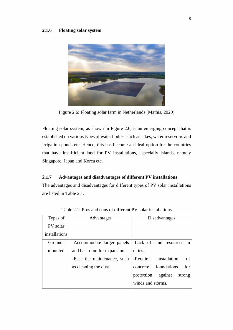
2.1.6 Floating solar system

Figure 2.6: Floating solar farm in Netherlands (Mathis, 2020)

Floating solar system, as shown in Figure 2.6, is an emerging concept that is

established on various types of water bodies, such as lakes, water reservoirs and

irrigation ponds etc. Hence, this has become an ideal option for the countries

that have insufficient land for PV installations, especially islands, namely

Singapore, Japan and Korea etc.

2.1.7 Advantages and disadvantages of different PV installations

The advantages and disadvantages for different types of PV solar installations

are listed in Table 2.1.

Table 2.1: Pros and cons of different PV solar installations

Types of

PV solar

installations

Advantages Disadvantages

Ground-

mounted

-Accommodate larger panels

and has room for expansion.

-Ease the maintenance, such

as cleaning the dust.

-Lack of land resources in

cities.

-Require installation of

concrete foundations for

protection against strong

winds and storms.

10

-Cutting down trees for large-

scale system

Rooftop -Does not require land space

and utilize the vacant roof

-The installation is relatively

faster and easier compared to

the ground-mounted type.

-Protect the roof and reduce

the temperature inside the

house by 35% or more

(Simpleray, n.d.).

-The roof space might restrict

solar panels.

-Probability of shading losses.

-Higher operating temperature

and, thus, lower performance.

Canal top -Conserve water by reducing

water evaporation.

-Save land space.

-Higher efficiency of solar

panels due to the cooling

water effect.

-Limited canals are available.

-More complex structures to

accommodate the panels.

-Hard for maintenance.

Offshore -Conserve land space.

-Increased efficiency of the

module as compared to land-

based.

-Less shading effect.

-Corrosion of solar panels due

to seawater.

-High maintenance cost.

-Difficult engineering works

due to the harsh conditions on

the sea.

BIPV -Save building materials and

labour cost.

-Can be used on structures that

cannot be installed with solar

panels.

-Difficult and expensive to

retrofit existing buildings.

-Lower efficiency as thin film

are usually used for BIPV

modules (Abhishek Shah,

2011).

11

Floating -Conserve land space.

-Conserve water by reducing

water evaporation.

-Enhance water quality by

preventing algae growth

-Higher module efficiency

due to the cooling effect of

water.

-Corrosion of the solar PV

components

-A barrier for transportation

and fishing activities (Dang

Anh Thi, 2017).

2.2 Components of floating solar PV system

The overall layout of a floating solar system is similar to the land-based solar

system. The main difference is that the PV arrays and sometimes the inverters

are mounted on a floating platform, as shown in Figure 2.7. The main

components in a floating solar PV system are floating system, mooring system,

solar PV system, cables, and connection.

Figure 2.7: Layout of floating solar system (Gamarra and Ronk, 2019)

2.2.1 Floating system

The floating system in the FSPV system consists of floats and pontoon. A

pontoon is a structure with the buoyancy that allows it to float with a heavy load.

It is a platform designed to hold an appropriate number of PV modules.

Meanwhile, floats are structures with effective buoyancy to its weight ratio, and

12

it is combined repeatedly to form a giant pontoon, as shown in Figure 2.8. The

floats are commonly made from high-density polyethylene, which is resistant to

sunlight and corrosion, has high tensile strength, and free from maintenance.

Figure 2.8: Float and pontoon structure (Sahu, Yadav and Sudhakar, 2016)

2.2.2 Mooring system

The mooring system in the FSPV system includes quays, anchor buoys, wharfs,

and mooring buoys. Its primary purpose is to maintain the solar panels in the

same position. The mooring system’s installation is done by tieing the nylon

wire rope slings to bollards on the bank and hooked at every corner, as shown

in Figure 2.9. Besides, there are three types of anchoring systems: bottom

anchoring, bank anchoring, and hybrid anchoring. The selection of anchoring

system relies on the site configuration and condition.

Figure 2.9: Mooring system for floating solar (Manoj Kumar, Kanchikere and

Mallikarjun, 2018)

13

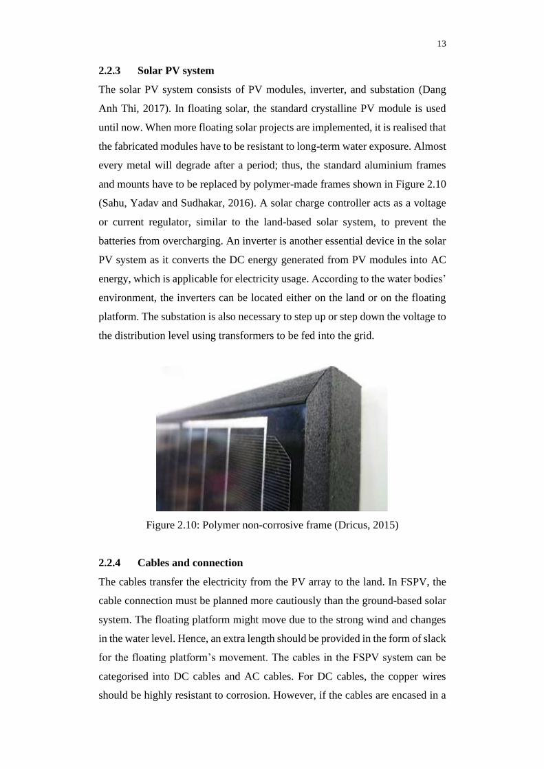
2.2.3 Solar PV system

The solar PV system consists of PV modules, inverter, and substation (Dang

Anh Thi, 2017). In floating solar, the standard crystalline PV module is used

until now. When more floating solar projects are implemented, it is realised that

the fabricated modules have to be resistant to long-term water exposure. Almost

every metal will degrade after a period; thus, the standard aluminium frames

and mounts have to be replaced by polymer-made frames shown in Figure 2.10

(Sahu, Yadav and Sudhakar, 2016). A solar charge controller acts as a voltage

or current regulator, similar to the land-based solar system, to prevent the

batteries from overcharging. An inverter is another essential device in the solar

PV system as it converts the DC energy generated from PV modules into AC

energy, which is applicable for electricity usage. According to the water bodies’

environment, the inverters can be located either on the land or on the floating

platform. The substation is also necessary to step up or step down the voltage to

the distribution level using transformers to be fed into the grid.

Figure 2.10: Polymer non-corrosive frame (Dricus, 2015)

2.2.4 Cables and connection

The cables transfer the electricity from the PV array to the land. In FSPV, the

cable connection must be planned more cautiously than the ground-based solar

system. The floating platform might move due to the strong wind and changes

in the water level. Hence, an extra length should be provided in the form of slack

for the floating platform’s movement. The cables in the FSPV system can be

categorised into DC cables and AC cables. For DC cables, the copper wires

should be highly resistant to corrosion. However, if the cables are encased in a

14

waterproof module junction box and are not in contact with water, regular DC

cables are applicable. Also, the AC cables should be resistant to high

temperatures and bad weather. There are two options for the cable routes. First,

the regular DC or AC cable can be lifted by floats on the water surface. Next,

the cables can be submerged through submarine cables, but this method is more

expensive (TERI, 2019).

2.2.5 Installation

The installation process of FSPV is more straightforward in terms of

construction because the building of mounting or supporting structures as in a

ground-mounted PV system is not required. The floating platform used in FSPV

is modular and prefabricated, so only the interconnection is needed to form a

larger segment. The floating platforms are usually assembled on land and are

pushed into the water when additional rows are added, as shown in Figure 2.11.

After the assembly is completed, the whole platform is pulled to the exact

location by boats. Hence, the deployment process usually takes a shorter time

as a comparison to the ground-mound PV system. For instance, a China leading

FSPV developer has reported that a 1 MWp FSPV system can be installed in

one day by 50 people (World Bank Group, ESMAP and SERIS, 2019).

Figure 2.11: Deployment ramp (World Bank Group, ESMAP and SERIS,

2019)

15

2.3 Advantages of floating solar technology

The benefits of the floating solar technology are listed as following with detailed

description and explanation.

2.3.1 Increased energy efficiency

Figure 2.12 Graph of efficiency against the photovoltaic module operational

temperature (Charles Lawrence et al., 2018)

The solar PV array’s energy yield is highly dependent on the solar cell

temperature and ambient temperature. Temperature is the primary factor that

contributes to thermal power losses. From Figure 2.12, the efficiency of the PV

module decreases linearly with its operational temperature. This research done

by Charles Lawrence et al. (2018) shows that the floating solar system has a

higher efficiency by 14.69 % based on an averaged module temperature of

21.95 °C. Another study carried out by International Energy Agency shows that

the energy losses related to temperature can vary between 1.7 % at 29 °C to

11.3 % at 51 °C (Nordmann and Clavadetscher, 2003). Due to the water’s

cooling effect, the ambient temperature and the PV module temperature

decreases. The wind speed above the water is higher than the land, resulting in

cooling the module. Therefore, the thermal losses of FSPV are lower. From this

aspect, the floating panels’ life span is also extended compared to the ground-

based solar system. Also, the usage of aluminium frames, which acts as the

mounting structure of the floatovoltaics, can further increase the efficiency by

transferring the cooler temperature on the water surface to the solar cell (Manoj

Kumar, Kanchikere and Mallikarjun, 2018). Some earlier floating solar projects

16

have reported an increased efficiency by more than 10 % by comparing to the

land-based solar system (Choi, Lee and Kim, 2013). There is also less shading

and soiling effect in the FSPV system, further increasing the energy yield.

2.3.2 Land conservation

Since the FSPV systems are located on the water bodies, it does not require any

land space. This benefit is essential for some countries whereby there is a lack

of land resources and limited roof space, such as Singapore and Japan. More

land space can be utilised for agricultural and industrial activities, which are

significant, especially in developing countries, namely India, Thailand, and

Malaysia. Meanwhile, the land cost escalates due to decreased land availability,

increasing the levelized tariff of electricity. Thus, FSPV also reduces an

enormous burden by saving high land costs. A techno-economic feasibility

study regarding a 10 MW FSPV plant shows that it has saved a land cost up to

USD 352125 and reduce the levelized tariff to USD 0.026kWh, which is lesser

than the land-based PV system by 39% (Goswami et al., 2019).

2.3.3 Reduced water evaporation

The installation of FSPV causes shading area on the water surface, leading to a

temperature drop of the water. By implementing FSPV on the water reservoirs,

it can reduce the water loss through evaporation. In the 2017 International

Floating Solar Symposium, there is a speech by Professor Eicke Weber, which

declares that the amount of water evaporation from the reservoirs is larger than

the human water consumption. Since the water loss on the reservoirs is

equivalent to a revenue loss, water evaporation reduction benefits the population

by reducing lost income and saving drinking water (Riding the wave of solar

energy: Why floating solar installations are a positive step for energy generation,

2018). Besides, Singapore’s National Water Agency PUB has planned to launch

a 50 MW floating solar plant on the Tengeh reservoir (Renewables Now, 2019)

and this floating solar will be operated by 2021.

2.3.4 Improved water quality

FSPV plants can improve water quality by inhibiting algae growth. The algae

growth is mainly depending on the light intensity and water temperature. By

17

having PV panels on the water surface, they prevent the sunlight from reaching

the water surface, preventing the algae growth.

2.3.5 Complementary operation with hydropower

The FSPV plants can be integrated with the hydropower stations to enhance the

power generation. The energy yield of the hydropower plant decreases during

the dry seasons because the water level drops. Meanwhile, the output of the

FSPV plant is intermittent due to the inconsistent solar irradiance. Hence, by

combining FSPV with the existing hydropower plants, the power production

variations are reduced, and the power quality is improved. This hybrid system’s

diurnal cycle can be optimized by having more solar power during the day and

more hydropower during the night time. The skilled staff at the hydropower site

and the data acquisition systems for existing hydropower plants can be utilized

for the newly built FSPV system. The nearby grid connections of the

hydropower plants can also link the FSPV to the grid, reducing the electrical

infrastructure’s investment cost (World Bank Group, ESMAP and SERIS,

2019).

2.4 Image processing techniques for calculation of irregular area

Several image processing techniques are studied and analyzed to be applied in

the lake area calculation in this project.

2.4.1 Monte Carlo simulation and image segmentation

Monte Carlo methods are primarily applied in solving mathematical problems

that involve several independent variables whereby plenty of memory and time

is needed for calculation through conventional methods. This method mainly

uses random samples of parameters to determine a complicated process; thus, it

is usually applied when it is impossible to calculate an exact solution. Therefore,

this Monte Carlo simulation can be utilised to approximate irregular area, such

as a lake. The procedures are listed as the following:

1) The irregular area is surrounded by a specified shape, namely rectangle,

triangle, or circle. Therefore, an appropriate shape is selected to confine

the interested region.

2) The individual point or input is scattered within the interested area.

18

3) Computation is performed on each input and later verify if the input is

within the irregular region or not.

4) The results of each input are combined at the end to obtain the estimation

of the irregular area.

Figure 2.13: Irregular area surrounded by rectangular shape (Obaid et al.,

2016)

Figure 2.14: Irregular area with darts (Obaid et al., 2016)

By considering an irregular shape image, the blue lake area, A, is

bounded by a white rectangle, R, as shown in Figure 2.13. By going through

Monte Carlo simulation, N black darts are spread randomly in a known area of

(𝐻 × 𝑊) as shown in Figure 2.14. 𝐻 is known as the height of the image, while

𝑊 is the width of the image. Assume K is the number of circle dots that are

found within the lake. By considering one dart in each pixel, the lake area is

expressed in Eq 2.1 (Obaid et al., 2016).

𝐿𝑎𝑘𝑒 𝑎𝑟𝑒𝑎, 𝐴 = 𝐾

𝑁𝑅 (2.1)

Scanned image analysis is needed in this method to differentiate the

desired objects from the background. An algorithm using the Visual Basic

19

program was created by Obaid et al. in 2016 to predict the scanned image area.

The program takes in an image and converts into matrix form according to a

given input threshold. The RGB values of each pixel are extracted to be saved

into a new matrix. The RGB values in each segmented image and the percentage

area covered by a specified color are computed. This method is suitable for

mapping any changes in land in general but not in a particular way (Obaid et al.,

2016).

2.4.2 Green’s Theorem

The area of an irregular region can be calculated through Green’s Theorem. By

taking a triangle, as shown in Figure 2.15, the area of the triangle can be

expressed as the Eq 2.2:

Let 𝑇1 = trapezoid with vertices (𝑥1, 𝑦1), (𝑥2, 𝑦2), (𝑥2, 0) 𝑎𝑛𝑑 (𝑥2, 0),

𝑇2 = trapezoid with vertices (𝑥2, 𝑦2), (𝑥3, 𝑦3), (𝑥3, 0) 𝑎𝑛𝑑 (𝑥2, 0),

𝑇3 = trapezoid with vertices (𝑥1, 𝑦1), (𝑥3, 𝑦3), (𝑥3, 0) 𝑎𝑛𝑑 (𝑥1, 0),

𝐴𝑟𝑒𝑎 = 𝑇1 + 𝑇2 − 𝑇3

=1

2(𝑦1 + 𝑦2)(𝑥2 − 𝑥1) +

1

2(𝑦2 + 𝑦3)(𝑥3 − 𝑥2) +

1

2(𝑦3 + 𝑦1)(𝑥1 − 𝑥3)

= −1

2(𝑥2𝑦3 − 𝑥3𝑦2 − 𝑥1𝑦3 + 𝑥3𝑦1 + 𝑥1𝑦2 − 𝑥2𝑦1)

= −1

2|

𝑥1 𝑦1 1𝑥2 𝑦2 1𝑥3 𝑦3 1

| (2.2)

Figure 2.15: A polygon with three vertices (Davis and Raianu, 2007)

Hence, the area of a polygon with vertices of (𝑥1, 𝑦1), (𝑥2, 𝑦2), … , (𝑥𝑛, 𝑦𝑛) in

clockwise orientation can be derived as:

20

𝐴𝑟𝑒𝑎 = 1

2∑(𝑦𝑖 + 𝑦𝑖+1)

𝑛−1

𝑖=1

(𝑥𝑖+1 − 𝑥𝑖) (2.3)

Moreover, the area’s formula stated in Eq 2.3 is a variation of the well known

Shoelace formula or Surveyor’s Formula in which the area can be expressed as:

𝐴𝑟𝑒𝑎 = 1

2∑ |

𝑥𝑖 𝑦𝑖

𝑥𝑖+1 𝑦𝑖+1|𝑛−1

𝑖=1 (2.4)

Davis and Rainu (2007) created a software planimeter to show the

application of Green’s Theorem. The program allows the user to upload an

image file and set the scale. Then, the user has to trace an enclosed region of the

image by using a mouse. The program then applies the Green’s Theorem to the

points obtained from the traced region, and the value of the areas calculated is

then shown to the user. The interpolating algorithms cannot improve the

accuracy of results obtained by using this program created. Besides, the

accuracy is highly dependent on the image accuracy and user’s hand-eye

coordination (Davis and Raianu, 2007).

2.4.3 Colour, contour,and shape detection using Open CV-Python

In 1999, Intel launched an Open Computer Vision Library (Open CV). Many

upgrades have been carried out for modifications to obtain a real-time computer

vision. This library is written under C and C++ programming languages but can

and can be interfaced with other programming languages easily, namely

MATLAB, Ruby and Python, etc.

This method requires the installation of Python software and Python

modules, such as and Matplotlib. First of all, the image is read using a

predefined function in Python, which is CV2.imread(). Several functions, such

as imread_color, imread_unchanged, and imread_grayscale, are also applicable.

The functions used to process the image consist of loading the image, detect the

shapes and colours inside the loaded image. It is widely used in object detection

applications, namely face recognition, accounting number of objects, and

automobile spotting (Puri and Gupta, 2018). Figure 2.16 has clearly stated the

steps for shape and colour detection in which shape detection employs contour

21

detection while colour detection employs pixel detection. For identifying the

lake area, colour detection is preferred as the lake’s shape differs from one

another. Meanwhile, the colour of the lake on the map is more consistent.

Figure 2.16: Simple flowchart of shape and colour detection (Puri and Gupta,

2018)

22

CHAPTER 3

3 METHODOLOGY AND WORK PLAN

3.1 General flow of the methodology

Figure 3.1 shows a simple flow of the project’s work plan. The first step is to

capture all the lakes in Selangor by using Google Map API key. The zoom level,

latitude, and longitude of the Google Map image are also adjusted in Python to

obtain a clear view of the lake. Next, all the lakes’ images are processed in

Python by using pixel and colour detection. The other water bodies on the image,

such as the river, are filtered out. The area of the lake is then calculated by

converting the unit from pixel to metre or kilometre. The floating solar system

is designed by considering several factors, such solar panels’ dimension,

Filter non-lake area on the image

Identify lake region

Calculate area of lake

Calculate PV capacity

Calculate first year electricity yield

Calculate Google Map image of lakes

Design the floating solar system

Figure 3.1: Simple flowchart of the work plan

23

number of panels per string and gaps between solar panels. The number of

panels installed on the lake is then calculated by assuming a reasonable lake

utilization rate. The annual electricity yield generated from the floating solar

plant on each lake is then calculated using the related formula. Lastly, the first-

year electricity yield generated from the floating solar plant on the lakes is

calculated.

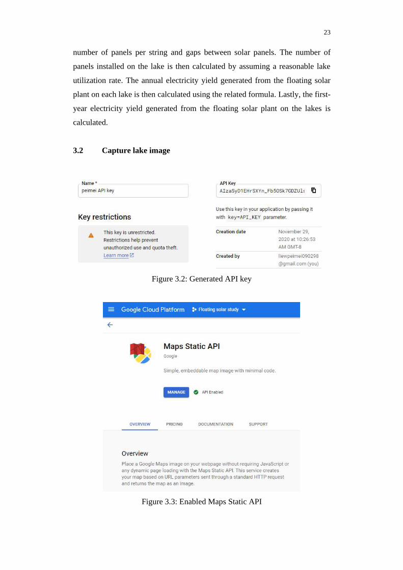
3.2 Capture lake image

Figure 3.2: Generated API key

Figure 3.3: Enabled Maps Static API

24

First of all, a Google API key is generated in Google Cloud Console, as shown

in Figure 3.2, to allow access with Google Services. The Maps Static API is

then enabled in the platform, as shown in Figure 3.3, to authenticate the request

of the Google Map image. For every request of the lake image, the lake’s

location, the size of the image and zoom level are stated clearly in the URL

encoding.

3.3 Detect water region, filter non-lake area and calculate lake area

After capturing all the lake images, some image processing techniques are

applied to identify the lake’s landscape and calculate the lakes’ area with scaling

factors.

The image processing of the Google Map image can be performed by

using contours in OpenCV of Python. Contours are a curve connecting all the

continuous points that have the same colour or intensity. Since the lake area is

in a constant blue colour, the lake area can be identified easily using this

OpenCV module.

First, the dependencies and necessary modules are installed and inserted

in Python IDLE, such as cv2 and NumPy. The steps are listed down as follows:

1) Read the map image by using cv2.imread() function.

2) Convert the image into a binary image in which every pixel of the

image is in black or white colour. The binary image is mandatory in

OpenCV because finding contours is the same as finding a white

object from a black background. The desired object must be in white

while the background is in black. In this project, the RGB pixel value

of the lake area is (170, 218, 255). Since the imread() function by

default interprets the image in BGR format, the pixel intensity value

is then written as (255, 218, 170). An upper and lower range of this

value is also specified to allow all the pixels that fall within this range

are identified and converted into white pixels.

3) Some of the lake images might consist of other water bodies. Hence,

these non-lake area is filtered out by using scikit-image module in

Python. The theory behind this is to extract the largest water body,

which is the lake. The small water region, like the river, is then

25

filtered. Besides, some lake area is made up of several regions; thus

the number of regions to be extracted from the image can also be

specified in the code.

4) After obtaining the desired lake region in the image, the number of

white pixels is counted using the countNonZero() function. The total

number of white pixels is equivalent to the lake area in unit pixels.

5) The lake area is then converted into unit metre by determining the

metre per pixel. The size of one pixel in unit metre is calculated by

using the Eq 3.1 below. This formula is based on the assumption that

the earth’s radius is 6378137 m.

𝑚𝑒𝑡𝑟𝑒 𝑝𝑒𝑟 𝑝𝑖𝑥𝑒𝑙 = 156543.03392 × cos (

𝑙𝑎𝑡𝑖𝑡𝑢𝑑𝑒 𝑜𝑓 𝑙𝑎𝑘𝑒 × 𝜋

180)

2𝑧𝑜𝑜𝑚 𝑙𝑒𝑣𝑒𝑙 (3.1)

6) The lake area in unit metre is then calculated by using the Eq 3.2

below.

𝑙𝑎𝑘𝑒 𝑎𝑟𝑒𝑎 = 𝑛𝑢𝑚𝑏𝑒𝑟 𝑜𝑓 𝑤ℎ𝑖𝑡𝑒 𝑝𝑖𝑥𝑒𝑙𝑠 × 𝑚𝑒𝑡𝑟𝑒 𝑝𝑒𝑟 𝑝𝑖𝑥𝑒𝑙 (3.2)

3.4 Calculation of PV capacity and annual electricity yield

After obtaining the area of lakes available in Selangor, the number of

solar panels on the lakes is then determined. Hence, the number of rows and

columns of solar panels is estimated by measuring the lakes’ width and lakes’

length. It is done by looping rows and columns of the pixels in the lake image.

For each row, the number of white pixels is counted and converted into the unit

metre to determine the lake’s width, if there is any. The lake’s width is then used

to calculate the number of strings of solar panels that can be fit into it. After

calculating the number of panels for the first row, the calculation proceeds to

the consecutive rows of the entire lake region. The total number of solar panels

for each row is summed up to calculate the PV capacity and annual electricity

yield. Some gaps between the adjacent solar panels in the same row and the

adjacent rows of solar panels are also considered. The calculation for the number

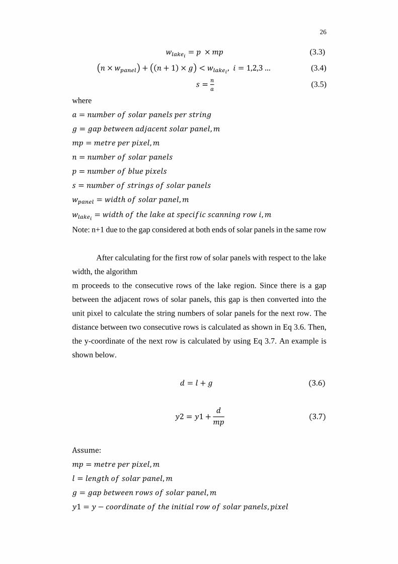
of strings of solar panels in the same row is shown in Eq 3.3 and Eq 3.4 below.

26

𝑤𝑙𝑎𝑘𝑒𝑖= 𝑝 × 𝑚𝑝 (3.3)

(𝑛 × 𝑤𝑝𝑎𝑛𝑒𝑙) + ((𝑛 + 1) × 𝑔) < 𝑤𝑙𝑎𝑘𝑒𝑖, 𝑖 = 1,2,3 … (3.4)

𝑠 =𝑛

𝑎 (3.5)

where

𝑎 = 𝑛𝑢𝑚𝑏𝑒𝑟 𝑜𝑓 𝑠𝑜𝑙𝑎𝑟 𝑝𝑎𝑛𝑒𝑙𝑠 𝑝𝑒𝑟 𝑠𝑡𝑟𝑖𝑛𝑔

𝑔 = 𝑔𝑎𝑝 𝑏𝑒𝑡𝑤𝑒𝑒𝑛 𝑎𝑑𝑗𝑎𝑐𝑒𝑛𝑡 𝑠𝑜𝑙𝑎𝑟 𝑝𝑎𝑛𝑒𝑙, 𝑚

𝑚𝑝 = 𝑚𝑒𝑡𝑟𝑒 𝑝𝑒𝑟 𝑝𝑖𝑥𝑒𝑙, 𝑚

𝑛 = 𝑛𝑢𝑚𝑏𝑒𝑟 𝑜𝑓 𝑠𝑜𝑙𝑎𝑟 𝑝𝑎𝑛𝑒𝑙𝑠

𝑝 = 𝑛𝑢𝑚𝑏𝑒𝑟 𝑜𝑓 𝑏𝑙𝑢𝑒 𝑝𝑖𝑥𝑒𝑙𝑠

𝑠 = 𝑛𝑢𝑚𝑏𝑒𝑟 𝑜𝑓 𝑠𝑡𝑟𝑖𝑛𝑔𝑠 𝑜𝑓 𝑠𝑜𝑙𝑎𝑟 𝑝𝑎𝑛𝑒𝑙𝑠

𝑤𝑝𝑎𝑛𝑒𝑙 = 𝑤𝑖𝑑𝑡ℎ 𝑜𝑓 𝑠𝑜𝑙𝑎𝑟 𝑝𝑎𝑛𝑒𝑙, 𝑚

𝑤𝑙𝑎𝑘𝑒𝑖= 𝑤𝑖𝑑𝑡ℎ 𝑜𝑓 𝑡ℎ𝑒 𝑙𝑎𝑘𝑒 𝑎𝑡 𝑠𝑝𝑒𝑐𝑖𝑓𝑖𝑐 𝑠𝑐𝑎𝑛𝑛𝑖𝑛𝑔 𝑟𝑜𝑤 𝑖, 𝑚

Note: n+1 due to the gap considered at both ends of solar panels in the same row

After calculating for the first row of solar panels with respect to the lake

width, the algorithm

m proceeds to the consecutive rows of the lake region. Since there is a gap

between the adjacent rows of solar panels, this gap is then converted into the

unit pixel to calculate the string numbers of solar panels for the next row. The

distance between two consecutive rows is calculated as shown in Eq 3.6. Then,

the y-coordinate of the next row is calculated by using Eq 3.7. An example is

shown below.

𝑑 = 𝑙 + 𝑔 (3.6)

𝑦2 = 𝑦1 +𝑑

𝑚𝑝 (3.7)

Assume:

𝑚𝑝 = 𝑚𝑒𝑡𝑟𝑒 𝑝𝑒𝑟 𝑝𝑖𝑥𝑒𝑙, 𝑚

𝑙 = 𝑙𝑒𝑛𝑔𝑡ℎ 𝑜𝑓 𝑠𝑜𝑙𝑎𝑟 𝑝𝑎𝑛𝑒𝑙, 𝑚

𝑔 = 𝑔𝑎𝑝 𝑏𝑒𝑡𝑤𝑒𝑒𝑛 𝑟𝑜𝑤𝑠 𝑜𝑓 𝑠𝑜𝑙𝑎𝑟 𝑝𝑎𝑛𝑒𝑙, 𝑚

𝑦1 = 𝑦 − 𝑐𝑜𝑜𝑟𝑑𝑖𝑛𝑎𝑡𝑒 𝑜𝑓 𝑡ℎ𝑒 𝑖𝑛𝑖𝑡𝑖𝑎𝑙 𝑟𝑜𝑤 𝑜𝑓 𝑠𝑜𝑙𝑎𝑟 𝑝𝑎𝑛𝑒𝑙𝑠, 𝑝𝑖𝑥𝑒𝑙

27

𝑦2 = 𝑦 − 𝑐𝑜𝑜𝑟𝑑𝑖𝑛𝑎𝑡𝑒 𝑜𝑓 𝑡ℎ𝑒 𝑛𝑒𝑥𝑡 𝑟𝑜𝑤 𝑜𝑓 𝑠𝑜𝑙𝑎𝑟 𝑝𝑎𝑛𝑒𝑙𝑠, 𝑝𝑖𝑥𝑒𝑙

𝑑 = 𝑝𝑖𝑡𝑐ℎ = 𝑡𝑜𝑡𝑎𝑙 𝑑𝑖𝑠𝑡𝑎𝑛𝑐𝑒 𝑏𝑒𝑡𝑤𝑒𝑒𝑛 𝑡ℎ𝑒 𝑡𝑤𝑜 𝑎𝑑𝑗𝑎𝑐𝑒𝑛𝑡 𝑟𝑜𝑤𝑠, 𝑚

When the number of strings of solar panels for each row is calculated,

the result is recorded to determine the respective lake’s PV capacity and annual

electricity yield. According to Dr Lim Boon Han, the performance ratio of solar

system in Malaysia is ranged from 80 % to 85 % and the peak sun hours in

Malaysia is around 1600 hours for a year. Hence, the performance ratio is set as

80 % and the peak sun hours for a year is set as 1600 hours in this study. The

PV capacity and the first-year electricity yield are calculated using Eq 3.8 and

Eq 3.9.

𝑃𝑉 =(𝑠 × 𝑛) × 𝑃

1 × 106 (3.8)

𝐸 = 𝑃𝑉 × 𝑃𝑆𝐻 × 𝑃𝑅 (3.9)

where

𝐸 = 𝐹𝑖𝑟𝑠𝑡 − 𝑦𝑒𝑎𝑟 𝑒𝑙𝑒𝑐𝑡𝑟𝑖𝑐𝑖𝑡𝑦 𝑔𝑒𝑛𝑒𝑟𝑎𝑡𝑖𝑜𝑛, 𝑀𝑊ℎ

𝑃𝑉 = 𝑃𝑉 𝑐𝑎𝑝𝑎𝑐𝑖𝑡𝑦, 𝑀𝑊

𝑠 = 𝑡𝑜𝑡𝑎𝑙 𝑛𝑢𝑚𝑏𝑒𝑟 𝑜𝑓 𝑠𝑡𝑟𝑖𝑛𝑔𝑠

𝑛 = 𝑛𝑢𝑚𝑏𝑒𝑟 𝑜𝑓 𝑠𝑜𝑙𝑎𝑟 𝑝𝑎𝑛𝑒𝑙𝑠 𝑝𝑒𝑟 𝑠𝑡𝑟𝑖𝑛𝑔

𝑃 = 𝑟𝑎𝑡𝑒𝑑 𝑝𝑜𝑤𝑒𝑟 𝑝𝑒𝑟 𝑝𝑎𝑛𝑒𝑙, 𝑊

𝑃𝑆𝐻 = 𝑃𝑒𝑎𝑘 𝑆𝑢𝑛 𝐻𝑜𝑢𝑟𝑠, ℎ𝑜𝑢𝑟𝑠

𝑃𝑅 = 𝑃𝑒𝑟𝑓𝑜𝑟𝑚𝑎𝑛𝑐𝑒 𝑅𝑎𝑡𝑖𝑜

After that, the annual electricity yield from each floating solar PV plant

on each lake in Selangor is summed up at the end to determine whether the

investment in floating solar is worthy or not. Meanwhile, the lake utilisation rate

is calculated to ensure it is less than 50 % to maintain a healthy ecosystem of all

the lakes. Since the lake area and the number of solar panels have been

determined in the previous steps, the lake utilization rate is computed using the

Eq 3.10 below. The specifications of the solar panels such as the size and rated

power are referred to Appendix D-1. The solar panels’ width and length in this

28

study are assumed to be 1.7 m and 1 m which are slightly higher than the value

in Appendix D-1 to include the area covered by the pontoons or floats.

Meanwhile, the structure of the floating system for this project is shown in

Appendix D-2, Appendix D-3 and Appendix D-4 (Lee, Joo and Yoon, 2014).

This system consists of Fiber-reinforced Polymer (FRP) material which results

in lesser number of buoys and lower volume immersed in the water bodies (Kim,

Yoon and Choi, 2017). However, the exact dimension of the floating structure

is not included in this study; thus, the lake utilization rate calculated is an

estimation.

𝐿 = 𝑁 × 𝑤 × 𝑙

𝐴× 100 (3.10)

where

𝐴 = 𝑙𝑎𝑘𝑒 𝑎𝑟𝑒𝑎, 𝑚

𝐿 = 𝑙𝑎𝑘𝑒 𝑢𝑡𝑖𝑙𝑖𝑠𝑎𝑡𝑖𝑜𝑛 𝑟𝑎𝑡𝑒, %

𝑁 = 𝑛𝑢𝑚𝑏𝑒𝑟 𝑜𝑓 𝑠𝑜𝑙𝑎𝑟 𝑝𝑎𝑛𝑒𝑙𝑠

𝑤 = 𝑤𝑖𝑑𝑡ℎ 𝑜𝑓 𝑠𝑜𝑙𝑎𝑟 𝑝𝑎𝑛𝑒𝑙, 𝑚

𝑙 = 𝑙𝑒𝑛𝑔𝑡ℎ 𝑜𝑓 𝑠𝑜𝑙𝑎𝑟 𝑝𝑎𝑛𝑒𝑙, 𝑚

The default image retrieved from the Google Cloud Platform has the

north direction pointing to the top, as shown in Figure 3.4. The algorithm

calculates the PV capacity from top left to top right; thus, the solar panel is

installed from north to south by default. For comparison, the lake image is

rotated to calculate the PV capacity in different directions, such as from south

to north, from west to east and from east to west. This is to determine whether

solar panels’ arrangement by different facing directions affects the PV capacity

calculated.

West

South

North

East

Figure 3.4: Default image direction

29

3.5 Verification of result

Several samples of lake images with a known size are created to go through the

Python algorithm. Three different shapes of lakes, such as rectangle, t-shape and

triangle, are created. All these shapes are created by stating a specified height

and width. For instance, the rectangle is created by stating a width of 200 pixels

and a height of 300 pixels. By controlling the input lake size, the PV capacity,

annual electricity yield and lake utilization rate are also manually calculated to

compare with the result from Python algorithm.

3.6 Work plan and Gantt Chart

3.6.1 Work plan

Table 3.1: Work plan with tasks and deadline

Category Activities Estimated

completion date

Identify project

scope and goals

-Identify the goals of the project.

-Define the project scope and list out all

the activities to achieve the goals.

28th June 2020

Research on

floating solar

and python

coding

-Research on the basic theory and

concept of floating solar.

-Research on the python coding to

calculate the area of lakes on google

map.

21th August

2020

Preliminary

testing on

python coding

-Progress report writing.

-Determine methods to calculate the

area of lakes, estimate the PV capacity

and energy yield.

-Preliminary testing or investigation for

calculation of lakes’ area using python.

13th September

2020

Capture map

images

-Save the map images of the lakes in

Selangor

22th January

2021

30

-Record the longitude, latitude and

zoom level of the image retrieved for

calculation later.

Calculate area

and number of

strings

-Compute the area, number of strings

of solar panels and the lake utilization

rate.

-Verify the result through control input

and manual calculation.

26th February

2021

Calculate annual

electricity yield

-Calculate and record the annual

electricity generated for the lakes in

Selangor.

5th March 2021

Trobleshoot and

further

enhancement

-Troubleshoot if there is any problem.

-A further enhancement is done if

necessary.

20 th March

2021

Final report and

presentation

-Final report writing and preparation

for presentation slides.

-Complete final report submission and

oral presentation of the project.

19 th April 2021

3.6.2 Gantt Chart

Figure 3.5: Gantt Chart of the project

15/6/2020 14/8/2020 13/10/202012/12/2020 10/2/2021 11/4/2021

Identify project scope and goals

Research on floating solar and python coding

Preliminary testing on python coding

Capture map images

Calculate area and number of strings

Calculate annual electricity yield

Troubleshoot and further enhancement

Final report and presentation

Start date Duration

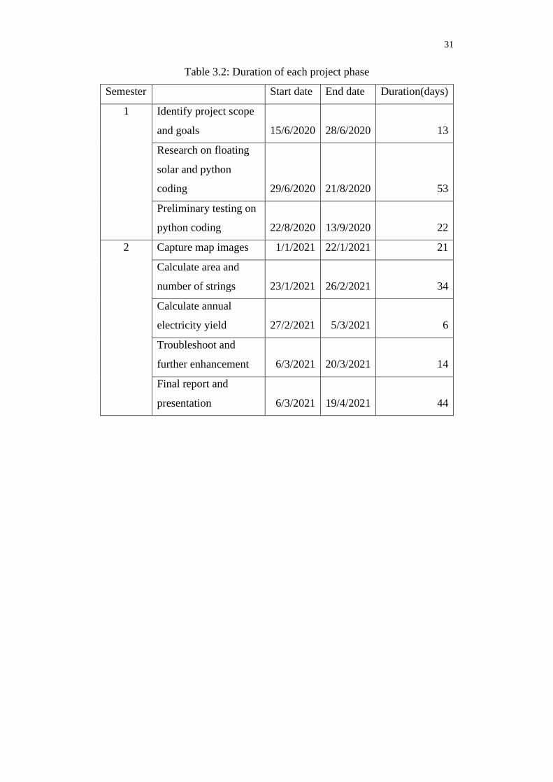
31

Table 3.2: Duration of each project phase

Semester

Start date End date Duration(days)

1 Identify project scope

and goals 15/6/2020 28/6/2020 13

Research on floating

solar and python

coding 29/6/2020 21/8/2020 53

Preliminary testing on

python coding 22/8/2020 13/9/2020 22

2 Capture map images 1/1/2021 22/1/2021 21

Calculate area and

number of strings 23/1/2021 26/2/2021 34

Calculate annual

electricity yield 27/2/2021 5/3/2021 6

Troubleshoot and

further enhancement 6/3/2021 20/3/2021 14

Final report and

presentation 6/3/2021 19/4/2021 44

32

CHAPTER 4

4 RESULTS AND DISCUSSION

The results and discussion are divided into several sections according to the

stage of project implementation. Firstly, the list of lake images is shown. The

zoom level and Earth coordinate to capture the images are also illustrated. After

applying image processing techniques such as contour and filtration, the

processed images are displayed to compare with the original images. The lake

area, PV capacity, and first-year electricity yield are also presented. The criteria

of the floating solar system designed are stated, such as the solar panels’

dimension and the gaps between the solar panels. Besides, all the Python codes

written to obtain the results are also illustrated.

4.1 Captured lake image and identified lake region

Figure 4.1: Code snippet to retrieve and save lake image

33

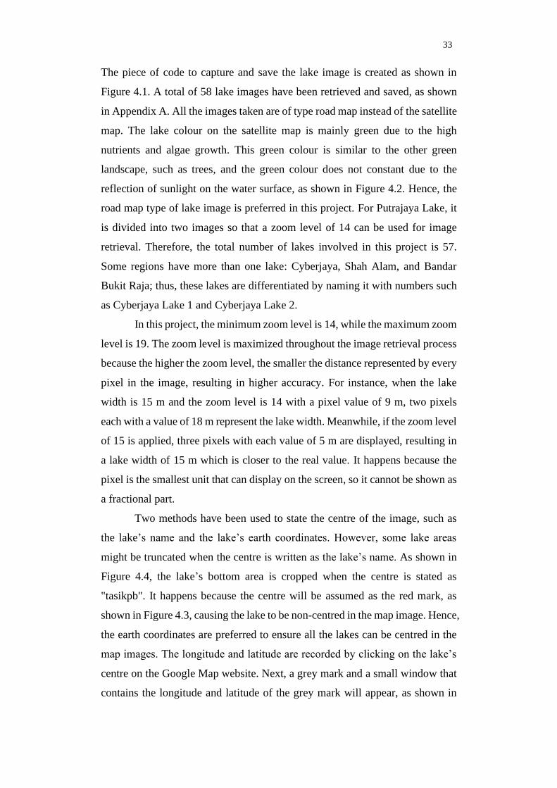
The piece of code to capture and save the lake image is created as shown in

Figure 4.1. A total of 58 lake images have been retrieved and saved, as shown

in Appendix A. All the images taken are of type road map instead of the satellite

map. The lake colour on the satellite map is mainly green due to the high

nutrients and algae growth. This green colour is similar to the other green

landscape, such as trees, and the green colour does not constant due to the

reflection of sunlight on the water surface, as shown in Figure 4.2. Hence, the

road map type of lake image is preferred in this project. For Putrajaya Lake, it

is divided into two images so that a zoom level of 14 can be used for image

retrieval. Therefore, the total number of lakes involved in this project is 57.

Some regions have more than one lake: Cyberjaya, Shah Alam, and Bandar

Bukit Raja; thus, these lakes are differentiated by naming it with numbers such

as Cyberjaya Lake 1 and Cyberjaya Lake 2.

In this project, the minimum zoom level is 14, while the maximum zoom

level is 19. The zoom level is maximized throughout the image retrieval process

because the higher the zoom level, the smaller the distance represented by every

pixel in the image, resulting in higher accuracy. For instance, when the lake

width is 15 m and the zoom level is 14 with a pixel value of 9 m, two pixels

each with a value of 18 m represent the lake width. Meanwhile, if the zoom level

of 15 is applied, three pixels with each value of 5 m are displayed, resulting in

a lake width of 15 m which is closer to the real value. It happens because the

pixel is the smallest unit that can display on the screen, so it cannot be shown as

a fractional part.

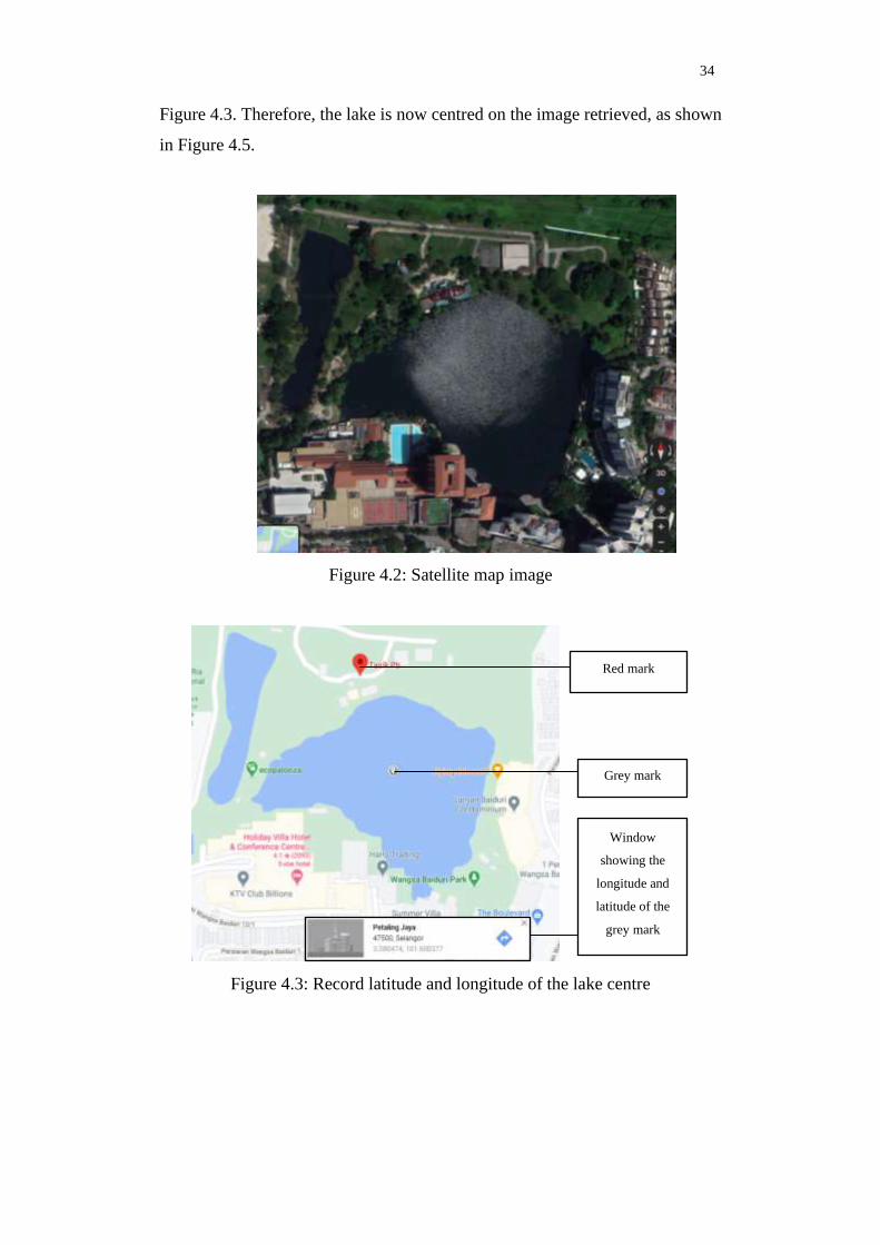
Two methods have been used to state the centre of the image, such as

the lake’s name and the lake’s earth coordinates. However, some lake areas

might be truncated when the centre is written as the lake’s name. As shown in

Figure 4.4, the lake’s bottom area is cropped when the centre is stated as

"tasikpb". It happens because the centre will be assumed as the red mark, as

shown in Figure 4.3, causing the lake to be non-centred in the map image. Hence,

the earth coordinates are preferred to ensure all the lakes can be centred in the

map images. The longitude and latitude are recorded by clicking on the lake’s

centre on the Google Map website. Next, a grey mark and a small window that

contains the longitude and latitude of the grey mark will appear, as shown in

34

Figure 4.3. Therefore, the lake is now centred on the image retrieved, as shown

in Figure 4.5.

Figure 4.2: Satellite map image

Figure 4.3: Record latitude and longitude of the lake centre

Red mark

Grey mark

Window

showing the

longitude and

latitude of the

grey mark

35

Figure 4.4: Truncated lake image when centre is written in terms of lake’s

name

Figure 4.5: Image obtained when centre is written in terms of longitude and

latitude

All the labels on the map image are also removed by turning off their

visibility in URL encoding. This prevents the wordings or marks on the usual

map image from covering some lake area and further decreasing the accuracy.

The zoom level and Earth coordinates are recorded and listed in Table 4.1 to

calculate metres per pixel.

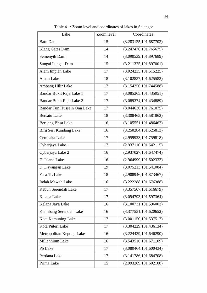
36

Table 4.1: Zoom level and coordinates of lakes in Selangor

Lake Zoom level Coordinates

Batu Dam 15 (3.283125,101.687703)

Klang Gates Dam 14 (3.247476,101.765675)

Semenyih Dam 14 (3.090539,101.897689)

Sungai Langat Dam 15 (3.211325,101.897001)

Alam Impian Lake 17 (3.024235,101.515225)

Aman Lake 18 (3.102837,101.625582)

Ampang Hilir Lake 17 (3.154256,101.744588)

Bandar Bukit Raja Lake 1 17 (3.085265,101.435051)

Bandar Bukit Raja Lake 2 17 (3.089374,101.434889)

Bandar Tun Hussein Onn Lake 17 (3.044636,101.761075)

Bersatu Lake 18 (3.308465,101.581862)

Beruang Bbsa Lake 16 (3.105551,101.486462)

Biru Seri Kundang Lake 16 (3.250284,101.525813)

Cempaka Lake 17 (2.959923,101.759818)

Cyberjaya Lake 1 17 (2.937110,101.642115)

Cyberjaya Lake 2 16 (2.937027,101.647474)

D' Island Lake 16 (2.964999,101.602333)

D' Kayangan Lake 19 (3.075213,101.541084)

Fasa 1L Lake 18 (2.908946,101.873467)

Indah Mewah Lake 16 (3.222288,101.676388)

Kebun Serendah Lake 17 (3.357507,101.616679)

Kelana Lake 17 (3.094793,101.597364)

Kelana Jaya Lake 16 (3.100731,101.596002)

Kiambang Serendah Lake 16 (3.377551,101.620652)

Kota Kemuning Lake 17 (3.001150,101.537512)

Kota Puteri Lake 17 (3.304229,101.436134)

Metropolitan Kepong Lake 16 (3.224439,101.646290)

Millennium Lake 16 (3.543516,101.671109)

Pb Lake 17 (3.080464,101.600434)

Perdana Lake 17 (3.141786,101.684708)

Prima Lake 15 (2.993269,101.602108)

37

Putrajaya Lake Part 1 14 (2.911117,101.682602)

Putrajaya Lake Part 2 14 (2.943847,101.695160)

Putra Perdana Lake 15 (2.954036,101.609220)

Residency Lake 15 (2.962581,101.590591)

Saujana Lake 18 (3.107370,101.577289)

Saujana Putra Lake 15 (2.945203,101.577110)

Seksyen 7 Lake 17 (3.077188,101.491932)

Semenyih Lake 16 (2.948359,101.861321)

Seri Aman Lake 17 (2.984084,101.584794)

Seri Serdang Lake 18 (3.004733,101.714276)

Serumpun Lake 19 (2.993416,101.715516)

Shah Alam Lake 1 17 (3.072088,101.514178)

Shah Alam Lake 2 17 (3.075928,101.516112)

Shah Alam Lake 3 18 (3.076252,101.520003)

Southlake Residence Lake 17 (3.067925,101.710795)

Sri Murni Lake 16 (3.235957,101.665081)

Sri Rampai Lake 17 (3.194879,101.728220)

Subang Dam 15 (3.175755,101.486245)

Sunway Lake 1 17 (3.062820,101.603509)

Sunway Lake 2 18 (3.069170,101.607232)

Sunway Serene Lake 17 (3.088246,101.605972)

Taman Dengkil Jaya Lake 17 (2.877000,101.672000)

Taman Subang Ria Lake 17 (3.082241,101.595698)

Teratai Lake 1 16 (2.938498,101.599512)

Teratai Lake 2 16 (2.930059,101.604933)

The Mines Lake 15 (3.035740,101.712057)

Titiwangsa Lake 16 (3.178547,101.707634)

38

Figure 4.6: Code snippet to convert the original map image into binary image

Figure 4.7: Code snippet to filter out non-lake regions

The code to convert the original map image into the binary image is

created, as shown in Figure 4.6. The water region is successfully differentiated

from the land region. However, it is found out that some map images have other

water bodies, such as a river, as shown in Figure 4.8, which results in an

inaccurate value of the lake area. Therefore, another piece of code is written, as

shown in Figure 4.7, to remove the non-lake area to increase the accuracy. The

area’s filtration is carried out by remaining the selected number of the largest

area in the image. Hence, some lake area that is not suitable for the installation

of solar panels is also eliminated. For instance, the middle part of Titiwangsa

Lake is not suited for panel installation, as shown in Figure 4.8; thus, it is

excluded and is ready for the calculation now, as shown in Figure 4.9. However,

it is only applicable to the lake divided into parts readily once the image is

retrieved from Google Maps. After converting the image into binary form and

39

removing the non-lake area, the 58 resulting lake images are shown in Appendix

B.

Figure 4.8: Lake Titiwangsa before image processing

Figure 4.9: Lake Titiwangsa after image processing

40

4.2 Lake area

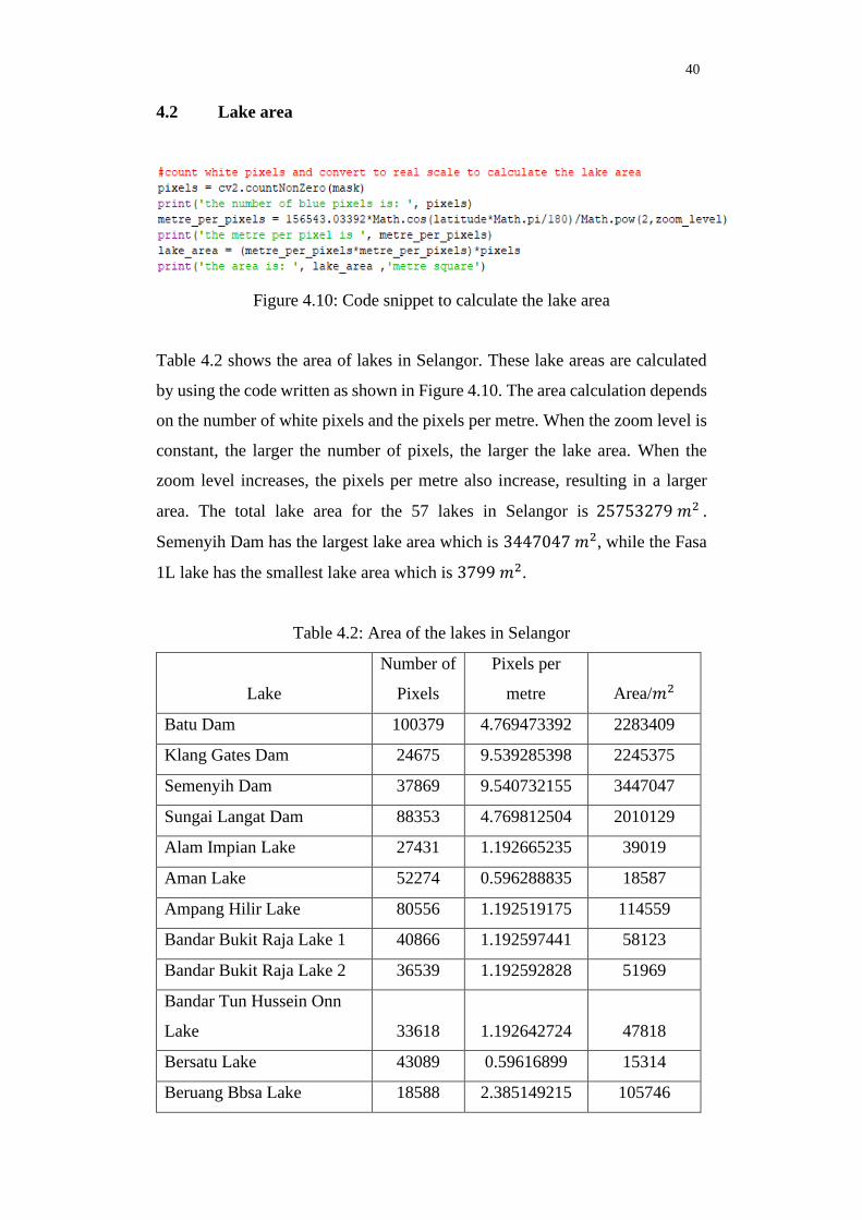
Figure 4.10: Code snippet to calculate the lake area

Table 4.2 shows the area of lakes in Selangor. These lake areas are calculated

by using the code written as shown in Figure 4.10. The area calculation depends

on the number of white pixels and the pixels per metre. When the zoom level is

constant, the larger the number of pixels, the larger the lake area. When the

zoom level increases, the pixels per metre also increase, resulting in a larger

area. The total lake area for the 57 lakes in Selangor is 25753279 𝑚2 .

Semenyih Dam has the largest lake area which is 3447047 𝑚2, while the Fasa

1L lake has the smallest lake area which is 3799 𝑚2.

Table 4.2: Area of the lakes in Selangor

Lake

Number of

Pixels

Pixels per

metre Area/𝑚2

Batu Dam 100379 4.769473392 2283409

Klang Gates Dam 24675 9.539285398 2245375

Semenyih Dam 37869 9.540732155 3447047

Sungai Langat Dam 88353 4.769812504 2010129

Alam Impian Lake 27431 1.192665235 39019

Aman Lake 52274 0.596288835 18587

Ampang Hilir Lake 80556 1.192519175 114559

Bandar Bukit Raja Lake 1 40866 1.192597441 58123

Bandar Bukit Raja Lake 2 36539 1.192592828 51969

Bandar Tun Hussein Onn

Lake 33618 1.192642724 47818

Bersatu Lake 43089 0.59616899 15314

Beruang Bbsa Lake 18588 2.385149215 105746

41

Biru Seri Kundang Lake 47781 2.384814715 271747

Cempaka Lake 36273 1.192735211 51603

Cyberjaya Lake 1 53542 1.192759672 76173

Cyberjaya Lake 2 38960 2.385519521 221710

D' Island Lake 130015 2.385459485 739840

D' Kayangan Lake 83339 0.298152175 7408

Fasa 1L Lake 10682 0.596394805 3799

Indah Mewah Lake 106713 2.384880605 606947

Kebun Serendah Lake 22129 1.192278547 31457

Kelana Lake 45018 1.192586735 64027

Kelana Jaya Lake 12995 2.385160093 73928

Kiambang Serendah Lake 42395 2.384508008 241053

Kota Kemuning Lake 49272 1.192690526 70090

Kota Puteri Lake 51550 1.192343073 73288

Metropolitan Kepong Lake 79155 2.384875563 450204

Millennium Lake 31917 2.384090366 181413

Pb Lake 45513 1.192602824 64733

Perdana Lake 26345 1.192533449 37466

Prima Lake 49953 4.770796464 1136955

Putrajaya Lake Part 1 28187 9.542298497 2566580

Putrajaya Lake Part 2 16082 9.542019743 1464268

Putra Perdana Lake 82763 4.770966165 1883861

Residency Lake 34243 4.770929395 779431

Saujana Lake 46244 0.596286276 16442

Saujana Putra Lake 36141 4.771004064 822659

Seksyen 7 Lake 62960 1.192606491 89549

Semenyih Lake 9370 2.385495268 53321

Seri Aman Lake 99813 1.192709099 141989

Seri Serdang Lake 48642 0.596343307 17298

Serumpun Lake 52797 0.298174739 4694

Shah Alam Lake 1 61279 1.192612193 87159

Shah Alam Lake 2 15952 1.192607901 22689

42

Shah Alam Lake 3 85971 0.596303769 30569

Southlake residence Lake 46963 1.192616841 66797

Sri Murni Lake 29927 2.384848505 170210

Sri Rampai Lake 15171 1.192472281 21573

Subang Dam 38410 4.769977727 873931

Sunway Lake 1 69331 1.192622531 98613

Sunway Lake 2 83927 0.596307726 29843

Sunway Serene Lake 30244 1.192594095 43015

Taman Dengkil Jaya Lake 117232 1.192823218 166801

Taman Subang Ria Lake 43382 1.192600832 61702

Teratai Lake 1 45726 2.385516378 260212

Teratai Lake 2 48588 2.385534388 276503

The Mines Lake 31754 4.770610235 722680

Titiwangsa Lake 24604 2.384982412 139951

4.3 PV Capacity, Annual Electricity Yield and Lake Utilization Rate

Figure 4.11: Code snippet to calculate number of panels, string number of solar

panels, lake utilization and annual electricity yield.

43

Table 4.3: PV capacity, annual electricity yield and lake utilization of lakes in

Selangor

Lake

Number

of

strings

PV

Capacity

/MW

Annual

Electricity

Yield /MWh

Lake

Utilization

Rate /%

Batu Dam 26956 161.736 207022.08 48.17

Klang Gates Dam 26353 158.118 202391.04 47.89

Semenyih Dam 40568 243.408 311562.24 48.02

Sungai Langat Dam 23840 143.04 183091.2 48.39

Alam Impian Lake 406 2.436 3118.08 42.45

Aman Lake 194 1.164 1489.92 42.59

Ampang Hilir Lake 1286 7.716 9876.48 45.8

Bandar Bukit Raja

Lake 1 602 3.612 4623.36 42.26

Bandar Bukit Raja

Lake 2 560 3.36 4300.8 43.97

Bandar Tun Hussein

Onn Lake 461 2.766 3540.48 39.33

Bersatu Lake 154 0.924 1182.72 41.03

Beruang Bbsa Lake 1096 6.576 8417.28 42.29

Biru Seri Kundang

Lake 3120 18.72 23961.6 46.84

Cempaka Lake 502 3.012 3855.36 39.69

Cyberjaya Lake 1 843 5.058 6474.24 45.15

Cyberjaya Lake 2 2507 15.042 19253.76 46.13

D' Island Lake 8617 51.702 66178.56 47.52

D' Kayangan Lake 68 0.408 522.24 37.45

Fasa 1L Lake 9 0.054 69.12 9.66

Indah Mewah Lake 7085 42.51 54412.8 47.63

Kebun Serendah

Lake 306 1.836 2350.08 39.69

Kelana Lake 684 4.104 5253.12 43.59

Kelana Jaya Lake 777 4.662 5967.36 42.88

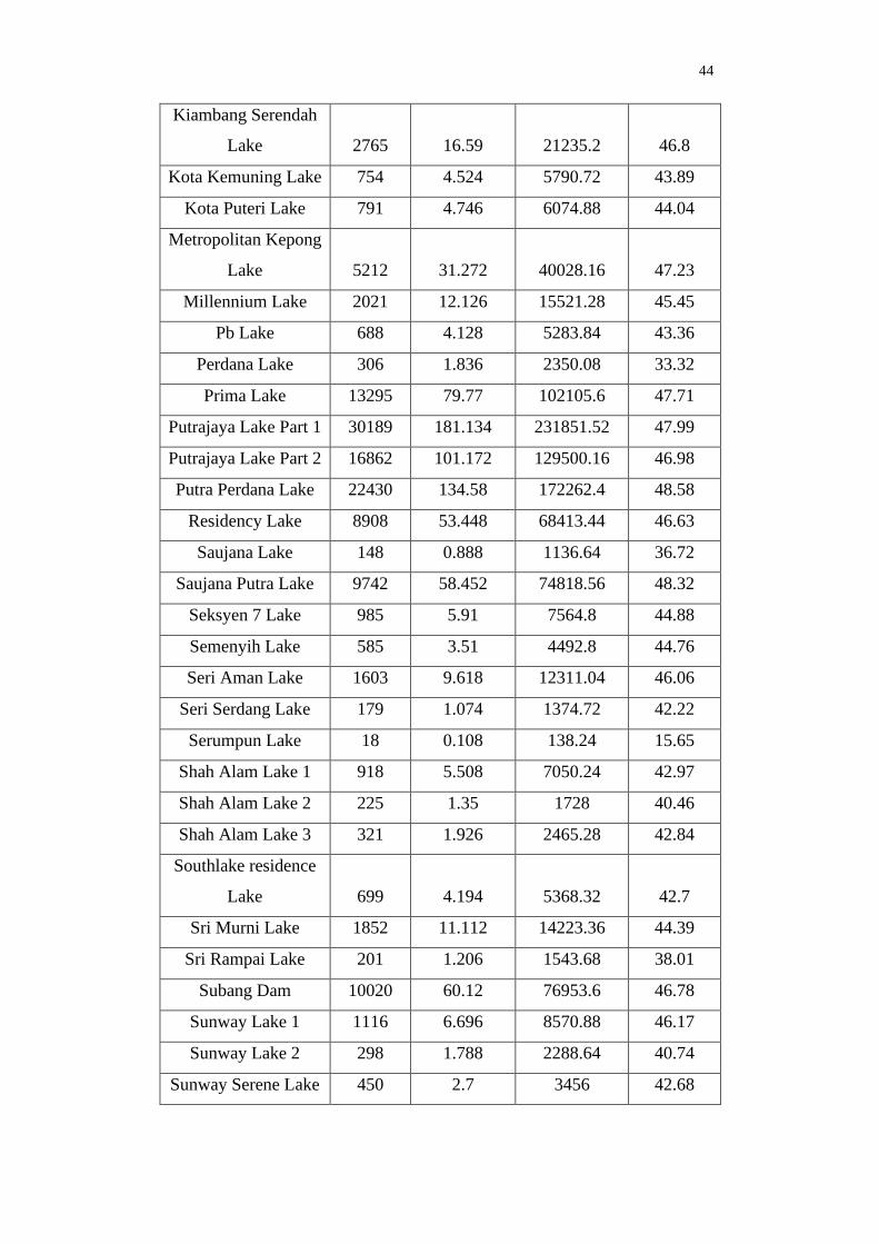
44

Kiambang Serendah

Lake 2765 16.59 21235.2 46.8

Kota Kemuning Lake 754 4.524 5790.72 43.89

Kota Puteri Lake 791 4.746 6074.88 44.04

Metropolitan Kepong

Lake 5212 31.272 40028.16 47.23

Millennium Lake 2021 12.126 15521.28 45.45

Pb Lake 688 4.128 5283.84 43.36

Perdana Lake 306 1.836 2350.08 33.32

Prima Lake 13295 79.77 102105.6 47.71

Putrajaya Lake Part 1 30189 181.134 231851.52 47.99

Putrajaya Lake Part 2 16862 101.172 129500.16 46.98

Putra Perdana Lake 22430 134.58 172262.4 48.58

Residency Lake 8908 53.448 68413.44 46.63

Saujana Lake 148 0.888 1136.64 36.72

Saujana Putra Lake 9742 58.452 74818.56 48.32

Seksyen 7 Lake 985 5.91 7564.8 44.88

Semenyih Lake 585 3.51 4492.8 44.76

Seri Aman Lake 1603 9.618 12311.04 46.06

Seri Serdang Lake 179 1.074 1374.72 42.22

Serumpun Lake 18 0.108 138.24 15.65

Shah Alam Lake 1 918 5.508 7050.24 42.97

Shah Alam Lake 2 225 1.35 1728 40.46

Shah Alam Lake 3 321 1.926 2465.28 42.84

Southlake residence

Lake 699 4.194 5368.32 42.7

Sri Murni Lake 1852 11.112 14223.36 44.39

Sri Rampai Lake 201 1.206 1543.68 38.01

Subang Dam 10020 60.12 76953.6 46.78

Sunway Lake 1 1116 6.696 8570.88 46.17

Sunway Lake 2 298 1.788 2288.64 40.74

Sunway Serene Lake 450 2.7 3456 42.68

45

Taman Dengkil Jaya

Lake 1840 11.04 14131.2 45.01

Taman Subang Ria

Lake 691 4.146 5306.88 45.69

Teratai Lake 1 2946 17.676 22625.28 46.19

Teratai Lake 2 3146 18.876 24161.28 46.42

The Mines Lake 8289 49.734 63659.52 46.8

Titiwangsa Lake 1581 9.486 12142.08 46.09

299068

(Total)

1794.408

(Total)

2296842.24

(Total)

43.15

(Average)

Figure 4.12: The criteria of floating solar system designed on the lakes

Figure 4.13: The results for each row of solar panels are printed with respect to

the lake width

46

As shown in Figure 4.11, the code is written to calculate the PV capacity on

each lake based on the floating solar system designed, as shown in Figure 4.12.

The results obtained are shown in Table 4.3. For every lake width of the lake,

the number of strings is calculated and printed out as shown in Figure 4.13.

Hence, the distribution and arrangement of solar panels on each lake can be

foreseen, and the number of strings is totalled up at the end to calculate PV

capacity. Since the number of solar panels per string in this project is 24, if the

lake width cannot fit in 24 panels each of dimension 1.7 𝑚 × 1 𝑚, then it will

be bypassed by the algorithm. Hence, the narrow lake length or width that is not

suitable for installing solar panels is omitted. During the design of rows of PV

array, it is a practice to specify a fixed number of solar panels for each row so

that it is easier to match the output power with the inverter size. For instance, if

the lake width can fit in 50 panels, the maximum number of strings of solar

panels will be 2, which is equivalent to 48 panels, and the remaining two panels

will be left out. The results without considering the number of panels per string

are also calculated, as shown in Appendix C-1. It is found out that the PV

capacity, annual electricity yield and lake utilisation rate, as shown in Appendix

C-1, are higher than those in Table 4.3. This happens because the number of

panels installed on the lakes is maximised without leaving out any solar panel.

Moreover, a gap of 0.02 m is allocated between the adjacent solar panels,

and another gap of 1 m is allocated between rows of solar panels. These gaps

mean to prevent potential shading issues that may lead to low performance of

the solar system and allow some space for expansion and contraction due to the

temperature. Besides, this arrangement of solar panels ensures that the lake

utilisation rate does not exceed 50 % to maintain a healthy ecosystem inside the

lakes.

Figure 4.14: Code snippet to rotate the default picture

47

In this project, the arrangement of solar panels is from north to south,

and, by default, the lake image retrieved have its top facing north. The solar

panels are chosen to face south because Malaysia is located in Northern

Malaysia; thus, the sun will be in the Southern sky throughout the year. The

solar panels are exposed to the sun for a longer period by facing south, resulting

in better performance. For comparison purpose, another three directions of solar

panels’ arrangement, such as south to north, west to east and east to west, are

also applied by using the code created as shown in Figure 4.14, and the results

are obtained as shown in Appendix C-2, Appendix C-3 and Appendix C-4. The

results from north to south direction are similar to south to north, as shown in

Table 4.3 and Appendix C-2. This happens because both directions have a

similar shape, and the difference is mainly caused by the different starting points,

as shown in Figure 4.15 and Figure 4.16. This situation is also applicable to the

direction of east to west and west to east, as shown in Figure 4.17 and Figure

4.18. These different results show that different facing directions of solar panels

and different starting points for installing solar panels would affect the PV

capacity calculated, further causing a difference in annual electricity yield and

lake utilisation rate.

Figure 4.15: Calculation of PV capacity from north to south

48

Figure 4.16: Calculation of PV capacity from south to north

Figure 4.17: Calculation of PV capacity from east to west

Figure 4.18: Calculation of PV capacity from west to east

The solar capacity in Malaysia has reached the value of 1493 MW in

2020 (IRENA, 2021). By installing the solar panels on lakes in Selangor, the

installed PV capacity can increase by 1794.408 MW, as shown in Table 4.3.,

resulting in a rise of 220 % in Malaysia’s total PV capacity. In Malaysia, the

49

long-term targets are 4000 MW of renewable capacity by the year 2030

(Annabeth, 2021). Hence, floating solar is a potential candidate in contributing

towards this target.

The total annual electricity generation from the floating solar system on

lakes in Selangor is around 2296.84 GWh, as shown in Table 4.3. This estimated

value is more than 522 % higher than the total annual electricity yield of solar

energy in 2018, which is 440 GWh.

Besides, the lake is not maximised in this study because it aims to

estimate the potential of floating solar capacity. Also, the lakes considered are

located in Selangor only, and the lake utilisation rate does not reach the

threshold of 50 %. Hence, there is still space for improvement of the floating

solar capacity.

4.4 Verification of result

First, the three lake samples with known size are created using the code written

as shown in Figure 4.19, Figure 4.20 and Figure 4.21. These lake images are set

as input to run through the algorithm in Python. The lake area, PV capacity and

first-year electricity generation are also calculated manually to verify whether

both results are similar.

Figure 4.19: Code snippet to create a known size of rectangular lake

50

Figure 4.20: Code snippet to create a known size of t-shaped lake

Figure 4.21: Code snippet to create a known size of right-angled triangle

4.4.1 Rectangular lake sample

4.4.1.1 Result from algorithm in Python using rectangular lake sample

The rectangular lake image created is shown in Figure 4.22, in which the white

rectangular shape represents the lake area. The parameters desired with their

units are calculated using the Python language, as shown in Figure 4.23.

Figure 4.22: Rectangular lake

51

Figure 4.23: Result from algorithm in Python using rectangular lake

4.4.1.2 Result from manual calculation using rectangular lake sample

Assume:

𝑧𝑜𝑜𝑚 𝑙𝑒𝑣𝑒𝑙 = 16, 𝑙𝑎𝑡𝑖𝑡𝑢𝑑𝑒 𝑜𝑓 𝑙𝑎𝑘𝑒 = 3.222288 ,

𝑔𝑎𝑝 𝑏𝑒𝑡𝑤𝑒𝑒𝑛 𝑎𝑑𝑗𝑎𝑐𝑒𝑛𝑡 𝑠𝑜𝑙𝑎𝑟 𝑝𝑎𝑛𝑒𝑙 = 0.02 𝑚,

𝑤𝑖𝑑𝑡ℎ 𝑜𝑓 𝑠𝑜𝑙𝑎𝑟 𝑝𝑎𝑛𝑒𝑙 = 1.7 𝑚, 𝑙𝑒𝑛𝑔𝑡ℎ 𝑜𝑓 𝑠𝑜𝑙𝑎𝑟 𝑝𝑎𝑛𝑒𝑙 = 1 𝑚

𝑚𝑒𝑡𝑟𝑒 𝑝𝑒𝑟 𝑝𝑖𝑥𝑒𝑙 = 156543.03392 × cos (

𝑙𝑎𝑡𝑖𝑡𝑢𝑑𝑒 𝑜𝑓 𝑙𝑎𝑘𝑒 × 𝜋

180)

2𝑧𝑜𝑜𝑚 𝑙𝑒𝑣𝑒𝑙

= 156543.03392 × cos (

3.222288 × 𝜋

180)

216= 2.384881

𝐺𝑎𝑝 𝑏𝑒𝑡𝑤𝑒𝑒𝑛 𝑟𝑜𝑤 𝑜𝑓 𝑝𝑎𝑛𝑒𝑙𝑠 = 2 𝑚𝑒𝑡𝑟𝑒 = 2 𝑚𝑒𝑡𝑟𝑒 × 1 𝑝𝑖𝑥𝑒𝑙

2.384881 𝑚𝑒𝑡𝑟𝑒

= 0.838616 𝑝𝑖𝑥𝑒𝑙

𝑙𝑎𝑘𝑒 𝑤𝑖𝑑𝑡ℎ = 2.384881 𝑚𝑒𝑡𝑟𝑒

𝑝𝑖𝑥𝑒𝑙 × 300 𝑝𝑖𝑥𝑒𝑙 = 715.4643 𝑚𝑒𝑡𝑟𝑒

𝑙𝑎𝑘𝑒 𝑙𝑒𝑛𝑔𝑡ℎ = 2.384881 𝑚𝑒𝑡𝑟𝑒

𝑝𝑖𝑥𝑒𝑙 × 250 𝑝𝑖𝑥𝑒𝑙 = 596.2202 𝑚𝑒𝑡𝑟𝑒

𝐿𝑎𝑘𝑒 𝑎𝑟𝑒𝑎 = 715.4643 × 596.2202 = 426574 𝑚2

Let 𝑛 = 𝑛𝑢𝑚𝑏𝑒𝑟 𝑜𝑓 𝑠𝑜𝑙𝑎𝑟 𝑝𝑎𝑛𝑒𝑙𝑠 𝑝𝑒𝑟 𝑟𝑜𝑤

(𝑛 × 1.7) + (𝑛 + 1) × 0.02 < 𝑙𝑎𝑘𝑒 𝑤𝑖𝑑𝑡ℎ

𝑛 < 𝑙𝑎𝑘𝑒 𝑤𝑖𝑑𝑡ℎ − 0.02

1.72

𝑛 < 715.4643 − 0.02

1.72

𝑛 < 415.96

Since n must be an integer, 𝑛 = 415

Since 𝑛𝑢𝑚𝑏𝑒𝑟 𝑜𝑓 𝑝𝑎𝑛𝑒𝑙𝑠 𝑝𝑒𝑟 𝑠𝑡𝑟𝑖𝑛𝑔 = 24 , 𝑛𝑢𝑚𝑏𝑒𝑟 𝑜𝑓 𝑠𝑡𝑟𝑖𝑛𝑔𝑠 =415

24=

17.29

Since number of strings must be an integer, 𝑛𝑢𝑚𝑏𝑒𝑟 𝑜𝑓 𝑠𝑡𝑟𝑖𝑛𝑔𝑠 = 17

52

𝑅𝑜𝑤𝑠 𝑜𝑓 𝑝𝑎𝑛𝑒𝑙𝑠, 𝑟 = 𝑙𝑎𝑘𝑒 ℎ𝑒𝑖𝑔ℎ𝑡

𝑔𝑎𝑝 𝑏𝑒𝑡𝑤𝑒𝑒𝑛 𝑟𝑜𝑤 𝑜𝑓 𝑝𝑎𝑛𝑒𝑙𝑠=

250 𝑝𝑖𝑥𝑒𝑙

0.838616 𝑝𝑖𝑥𝑒𝑙

= 596.2202 𝑚

2 𝑚= 298.11

Since r must be an integer, 𝑟 = 298

𝑇𝑜𝑡𝑎𝑙 𝑛𝑢𝑚𝑏𝑒𝑟 𝑜𝑓 𝑝𝑎𝑛𝑒𝑙𝑠

= 𝑟 × 𝑛𝑢𝑚𝑏𝑒𝑟 𝑜𝑓 𝑠𝑡𝑟𝑖𝑛𝑔𝑠 × 𝑛𝑢𝑚𝑏𝑒𝑟 𝑜𝑓 𝑝𝑎𝑛𝑒𝑙𝑠 𝑝𝑒𝑟 𝑠𝑡𝑟𝑖𝑛𝑔

= 298 × 17 × 24 = 121584

𝑇𝑜𝑡𝑎𝑙 𝑛𝑢𝑚𝑏𝑒𝑟 𝑜𝑓 𝑠𝑡𝑟𝑖𝑛𝑔𝑠 = 𝑟 × 𝑛𝑢𝑚𝑏𝑒𝑟 𝑜𝑓 𝑠𝑡𝑟𝑖𝑛𝑔𝑠 = 5066

𝑃𝑉 𝑐𝑎𝑝𝑎𝑐𝑖𝑡𝑦 = 𝑛𝑢𝑚𝑏𝑒𝑟 𝑜𝑓 𝑝𝑎𝑛𝑒𝑙𝑠 × 𝑟𝑎𝑡𝑒𝑑 𝑝𝑜𝑤𝑒𝑟 𝑝𝑒𝑟 𝑝𝑎𝑛𝑒𝑙

= 121584 × 250 𝑊 = 30.396 𝑀𝑊

𝐴𝑛𝑛𝑢𝑎𝑙 𝑒𝑙𝑒𝑐𝑡𝑟𝑖𝑐𝑖𝑡𝑦 𝑦𝑖𝑒𝑙𝑑

= 𝑡𝑜𝑡𝑎𝑙 𝑛𝑢𝑚𝑏𝑒𝑟 𝑜𝑓 𝑝𝑎𝑛𝑒𝑙𝑠 × 𝑟𝑎𝑡𝑒𝑑 𝑝𝑜𝑤𝑒𝑟 𝑝𝑒𝑟 𝑝𝑎𝑛𝑒𝑙 ×

𝑝𝑒𝑎𝑘 𝑠𝑢𝑛 ℎ𝑜𝑢𝑟𝑠 𝑝𝑒𝑟 𝑦𝑒𝑎𝑟 × 𝑝𝑒𝑟𝑓𝑜𝑟𝑚𝑎𝑛𝑐𝑒 𝑟𝑎𝑡𝑖𝑜

= 121584 × 250 × 1600 × 0.8

= 38906.88 𝑀𝑊ℎ

𝐿𝑎𝑘𝑒 𝑢𝑡𝑖𝑙𝑖𝑧𝑎𝑡𝑖𝑜𝑛 𝑟𝑎𝑡𝑒 =𝑡𝑜𝑡𝑎𝑙 𝑛𝑢𝑚𝑏𝑒𝑟 𝑜𝑓 𝑠𝑜𝑙𝑎𝑟 𝑝𝑎𝑛𝑒𝑙𝑠×𝑎𝑟𝑒𝑎 𝑜𝑓 𝑎 𝑠𝑜𝑙𝑎𝑟 𝑝𝑎𝑛𝑒𝑙

𝑙𝑎𝑘𝑒 𝑎𝑟𝑒𝑎=

121584×(1 𝑚 × 1.7 𝑚)

426574 𝑚2 = 48.45 %

4.4.1.3 Comparison of results obtained from two methods using

rectangular lake sample

Table 4.4: Comparison of results using rectangular lake sample

Python algorithm Manual calculation

Lake area (𝑚2) 426574 426574

Number of strings of panels 5066 5066

PV Capacity (MW) 30.396 30.396

Annual electricity yield (MWh) 38906.88 38906.88

Lake utilization rate (%) 48.45 48.45

From Table 4.4, the results obtained from the Python algorithm and manual

calculation are the same. Therefore, by controlling the input as a fixed

rectangular shape, the algorithm works in the desired way.

53

4.4.2 T-shaped lake sample

4.4.2.1 Result from algorithm in Python using t-shaped lake sample

The t-shaped lake is created as shown in Figure 4.24, with the lake’s dimensions

illustrated. The results obtained using the t-shaped lake image as input are also

shown in Figure 4.25.

Figure 4.24: T-shaped lake

Figure 4.25: Result from algorithm in Python using t-shaped lake

4.4.2.2 Result from manual calculation for t-shaped lake sample

Assume:

𝑧𝑜𝑜𝑚 𝑙𝑒𝑣𝑒𝑙 = 14, 𝑙𝑎𝑡𝑖𝑡𝑢𝑑𝑒 𝑜𝑓 𝑙𝑎𝑘𝑒 = 3.178178 ,

𝑔𝑎𝑝 𝑏𝑒𝑡𝑤𝑒𝑒𝑛 𝑎𝑑𝑗𝑎𝑐𝑒𝑛𝑡 𝑠𝑜𝑙𝑎𝑟 𝑝𝑎𝑛𝑒𝑙 = 0.02 𝑚,

𝑤𝑖𝑑𝑡ℎ 𝑜𝑓 𝑠𝑜𝑙𝑎𝑟 𝑝𝑎𝑛𝑒𝑙 = 1.7 𝑚, 𝑙𝑒𝑛𝑔𝑡ℎ 𝑜𝑓 𝑠𝑜𝑙𝑎𝑟 𝑝𝑎𝑛𝑒𝑙 = 1 𝑚

𝑚𝑒𝑡𝑟𝑒 𝑝𝑒𝑟 𝑝𝑖𝑥𝑒𝑙 = 156543.03392 × cos (

𝑙𝑎𝑡𝑖𝑡𝑢𝑑𝑒 𝑜𝑓 𝑙𝑎𝑘𝑒 × 𝜋

180)

2𝑧𝑜𝑜𝑚 𝑙𝑒𝑣𝑒𝑙

= 156543.03392 × cos (

3.178178 × 𝜋

180)

214= 9.539933

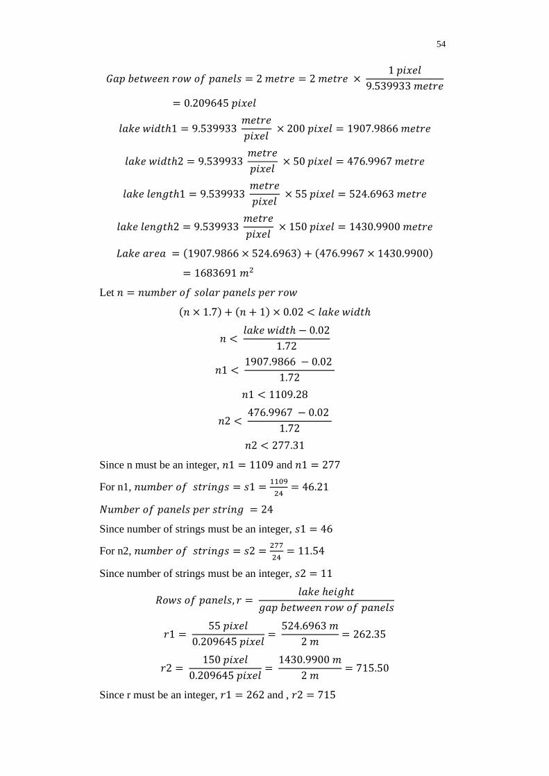
54

𝐺𝑎𝑝 𝑏𝑒𝑡𝑤𝑒𝑒𝑛 𝑟𝑜𝑤 𝑜𝑓 𝑝𝑎𝑛𝑒𝑙𝑠 = 2 𝑚𝑒𝑡𝑟𝑒 = 2 𝑚𝑒𝑡𝑟𝑒 × 1 𝑝𝑖𝑥𝑒𝑙

9.539933 𝑚𝑒𝑡𝑟𝑒

= 0.209645 𝑝𝑖𝑥𝑒𝑙

𝑙𝑎𝑘𝑒 𝑤𝑖𝑑𝑡ℎ1 = 9.539933 𝑚𝑒𝑡𝑟𝑒

𝑝𝑖𝑥𝑒𝑙 × 200 𝑝𝑖𝑥𝑒𝑙 = 1907.9866 𝑚𝑒𝑡𝑟𝑒

𝑙𝑎𝑘𝑒 𝑤𝑖𝑑𝑡ℎ2 = 9.539933 𝑚𝑒𝑡𝑟𝑒

𝑝𝑖𝑥𝑒𝑙 × 50 𝑝𝑖𝑥𝑒𝑙 = 476.9967 𝑚𝑒𝑡𝑟𝑒

𝑙𝑎𝑘𝑒 𝑙𝑒𝑛𝑔𝑡ℎ1 = 9.539933 𝑚𝑒𝑡𝑟𝑒

𝑝𝑖𝑥𝑒𝑙 × 55 𝑝𝑖𝑥𝑒𝑙 = 524.6963 𝑚𝑒𝑡𝑟𝑒

𝑙𝑎𝑘𝑒 𝑙𝑒𝑛𝑔𝑡ℎ2 = 9.539933 𝑚𝑒𝑡𝑟𝑒

𝑝𝑖𝑥𝑒𝑙 × 150 𝑝𝑖𝑥𝑒𝑙 = 1430.9900 𝑚𝑒𝑡𝑟𝑒

𝐿𝑎𝑘𝑒 𝑎𝑟𝑒𝑎 = (1907.9866 × 524.6963) + (476.9967 × 1430.9900)

= 1683691 𝑚2

Let 𝑛 = 𝑛𝑢𝑚𝑏𝑒𝑟 𝑜𝑓 𝑠𝑜𝑙𝑎𝑟 𝑝𝑎𝑛𝑒𝑙𝑠 𝑝𝑒𝑟 𝑟𝑜𝑤

(𝑛 × 1.7) + (𝑛 + 1) × 0.02 < 𝑙𝑎𝑘𝑒 𝑤𝑖𝑑𝑡ℎ

𝑛 < 𝑙𝑎𝑘𝑒 𝑤𝑖𝑑𝑡ℎ − 0.02

1.72

𝑛1 < 1907.9866 − 0.02

1.72

𝑛1 < 1109.28

𝑛2 < 476.9967 − 0.02

1.72

𝑛2 < 277.31

Since n must be an integer, 𝑛1 = 1109 and 𝑛1 = 277

For n1, 𝑛𝑢𝑚𝑏𝑒𝑟 𝑜𝑓 𝑠𝑡𝑟𝑖𝑛𝑔𝑠 = 𝑠1 =1109

24= 46.21

𝑁𝑢𝑚𝑏𝑒𝑟 𝑜𝑓 𝑝𝑎𝑛𝑒𝑙𝑠 𝑝𝑒𝑟 𝑠𝑡𝑟𝑖𝑛𝑔 = 24

Since number of strings must be an integer, 𝑠1 = 46

For n2, 𝑛𝑢𝑚𝑏𝑒𝑟 𝑜𝑓 𝑠𝑡𝑟𝑖𝑛𝑔𝑠 = 𝑠2 =277

24= 11.54

Since number of strings must be an integer, 𝑠2 = 11

𝑅𝑜𝑤𝑠 𝑜𝑓 𝑝𝑎𝑛𝑒𝑙𝑠, 𝑟 = 𝑙𝑎𝑘𝑒 ℎ𝑒𝑖𝑔ℎ𝑡

𝑔𝑎𝑝 𝑏𝑒𝑡𝑤𝑒𝑒𝑛 𝑟𝑜𝑤 𝑜𝑓 𝑝𝑎𝑛𝑒𝑙𝑠

𝑟1 = 55 𝑝𝑖𝑥𝑒𝑙

0.209645 𝑝𝑖𝑥𝑒𝑙=

524.6963 𝑚

2 𝑚= 262.35

𝑟2 = 150 𝑝𝑖𝑥𝑒𝑙

0.209645 𝑝𝑖𝑥𝑒𝑙=

1430.9900 𝑚

2 𝑚= 715.50

Since r must be an integer, 𝑟1 = 262 and , 𝑟2 = 715

55

Since 262.35 + 715.50 − 262 − 715 < 1, there is no extra row that can be

formed.

𝑇𝑜𝑡𝑎𝑙 𝑛𝑢𝑚𝑏𝑒𝑟 𝑜𝑓 𝑝𝑎𝑛𝑒𝑙𝑠

= 𝑟 × 𝑛𝑢𝑚𝑏𝑒𝑟 𝑜𝑓 𝑠𝑡𝑟𝑖𝑛𝑔𝑠 × 𝑛𝑢𝑚𝑏𝑒𝑟 𝑜𝑓 𝑝𝑎𝑛𝑒𝑙𝑠 𝑝𝑒𝑟 𝑠𝑡𝑟𝑖𝑛𝑔

= (𝑟1 × 𝑠1 × 24) + (𝑟2 × 𝑠2 × 24)

= (262 × 46 × 24) + (715 × 11 × 24) = 478008

𝑇𝑜𝑡𝑎𝑙 𝑛𝑢𝑚𝑏𝑒𝑟 𝑜𝑓 𝑠𝑡𝑟𝑖𝑛𝑔𝑠 = 𝑟 × 𝑛𝑢𝑚𝑏𝑒𝑟 𝑜𝑓 𝑠𝑡𝑟𝑖𝑛𝑔𝑠

= (𝑟1 × 𝑠1) + (𝑟2 × 𝑠2) = (262 × 46) + (715 × 11)

= 19917

𝑃𝑉 𝑐𝑎𝑝𝑎𝑐𝑖𝑡𝑦 = 𝑛𝑢𝑚𝑏𝑒𝑟 𝑜𝑓 𝑝𝑎𝑛𝑒𝑙𝑠 × 𝑟𝑎𝑡𝑒𝑑 𝑝𝑜𝑤𝑒𝑟 𝑝𝑒𝑟 𝑝𝑎𝑛𝑒𝑙

= 478008 × 250 𝑊 = 119.502 𝑀𝑊

𝐴𝑛𝑛𝑢𝑎𝑙 𝑒𝑙𝑒𝑐𝑡𝑟𝑖𝑐𝑖𝑡𝑦 𝑦𝑖𝑒𝑙𝑑

= 𝑡𝑜𝑡𝑎𝑙 𝑛𝑢𝑚𝑏𝑒𝑟 𝑜𝑓 𝑝𝑎𝑛𝑒𝑙𝑠 × 𝑟𝑎𝑡𝑒𝑑 𝑝𝑜𝑤𝑒𝑟 𝑝𝑒𝑟 𝑝𝑎𝑛𝑒𝑙 ×

𝑝𝑒𝑎𝑘 𝑠𝑢𝑛 ℎ𝑜𝑢𝑟𝑠 𝑝𝑒𝑟 𝑦𝑒𝑎𝑟 × 𝑝𝑒𝑟𝑓𝑜𝑟𝑚𝑎𝑛𝑐𝑒 𝑟𝑎𝑡𝑖𝑜

= 478008 × 250 × 1600 × 0.8 = 152962.56 𝑀𝑊ℎ

𝐿𝑎𝑘𝑒 𝑢𝑡𝑖𝑙𝑖𝑧𝑎𝑡𝑖𝑜𝑛 𝑟𝑎𝑡𝑒 =𝑡𝑜𝑡𝑎𝑙 𝑛𝑢𝑚𝑏𝑒𝑟 𝑜𝑓 𝑠𝑜𝑙𝑎𝑟 𝑝𝑎𝑛𝑒𝑙𝑠×𝑎𝑟𝑒𝑎 𝑜𝑓 𝑎 𝑠𝑜𝑙𝑎𝑟 𝑝𝑎𝑛𝑒𝑙

𝑙𝑎𝑘𝑒 𝑎𝑟𝑒𝑎=

478008×(1 𝑚 × 1.7 𝑚)

1683691 𝑚2 = 48.26 %

4.4.2.3 Comparison of results obtained from two methods using t-shaped

lake sample

Table 4.5: Comparison of results using t-shaped lake sample

Python algorithm Manual calculation

Lake area (𝑚2) 1683691 1683691

Number of strings of panels 19917 19917

PV Capacity (MW) 119.502 119.502

Annual electricity yield (MWh) 152962.56 152962.56

Lake utilization rate (%) 48.26 48.26

From Table 4.5, the results obtained from the algorithm in Python and the

manual calculation are the same. This has shown that the algorithm is working

correctly for the t-shaped lake sample.

56

4.4.3 Triangular lake sample

4.4.3.1 Result from algorithm in Python using triangular lake sample

Moreover, another lake sample with a triangular shape is also created. For this

shape, the lake width changes for every calculation, as shown in Figure 4.26.

The parameters calculated with two different scales are also shown in Figure

4.27 and Figure 4.28.

Figure 4.26: Triangular lake

Figure 4.27: Result from algorithm in Python using triangular lake with a scale

of 2 metre per pixel

Figure 4.28: Result from algorithm in Python using triangular lake with a scale

of 4 metre per pixel

57

4.4.3.2 Result from manual calculation for triangular lake sample

Since the triangular lake sample has its length and width keeps changing, the

calculation is made to be simpler by assuming scale the scale which is metre per

pixel of the image as an integer. Meanwhile, this sample is tested using two

scales, such as 2 metres per pixel and 4 metres per pixel.

Assume:

𝑔𝑎𝑝 𝑏𝑒𝑡𝑤𝑒𝑒𝑛 𝑎𝑑𝑗𝑎𝑐𝑒𝑛𝑡 𝑠𝑜𝑙𝑎𝑟 𝑝𝑎𝑛𝑒𝑙 = 0.02 𝑚,

𝑤𝑖𝑑𝑡ℎ 𝑜𝑓 𝑠𝑜𝑙𝑎𝑟 𝑝𝑎𝑛𝑒𝑙 = 1.7 𝑚, 𝑙𝑒𝑛𝑔𝑡ℎ 𝑜𝑓 𝑠𝑜𝑙𝑎𝑟 𝑝𝑎𝑛𝑒𝑙 = 1 𝑚

When 𝑚𝑒𝑡𝑟𝑒 𝑝𝑒𝑟 𝑝𝑖𝑥𝑒𝑙 = 2

𝐺𝑎𝑝 𝑏𝑒𝑡𝑤𝑒𝑒𝑛 𝑟𝑜𝑤 𝑜𝑓 𝑝𝑎𝑛𝑒𝑙𝑠 = 2 𝑚𝑒𝑡𝑟𝑒 = 2 𝑚𝑒𝑡𝑟𝑒 × 1 𝑝𝑖𝑥𝑒𝑙

2 𝑚𝑒𝑡𝑟𝑒= 1 𝑝𝑖𝑥𝑒𝑙

𝑙𝑎𝑘𝑒 𝑤𝑖𝑑𝑡ℎ = 2 𝑚𝑒𝑡𝑟𝑒

𝑝𝑖𝑥𝑒𝑙 × 60 𝑝𝑖𝑥𝑒𝑙 = 120 𝑚𝑒𝑡𝑟𝑒

𝑙𝑎𝑘𝑒 𝑙𝑒𝑛𝑔𝑡ℎ = 2 𝑚𝑒𝑡𝑟𝑒

𝑝𝑖𝑥𝑒𝑙 × 60 𝑝𝑖𝑥𝑒𝑙 = 120 𝑚𝑒𝑡𝑟𝑒

𝐿𝑎𝑘𝑒 𝑎𝑟𝑒𝑎 =1

2(120 × 120 ) = 7200 𝑚2

When 𝑚𝑒𝑡𝑟𝑒 𝑝𝑒𝑟 𝑝𝑖𝑥𝑒𝑙 = 4

𝐺𝑎𝑝 𝑏𝑒𝑡𝑤𝑒𝑒𝑛 𝑟𝑜𝑤 𝑜𝑓 𝑝𝑎𝑛𝑒𝑙𝑠 = 2 𝑚𝑒𝑡𝑟𝑒 = 2 𝑚𝑒𝑡𝑟𝑒 × 1 𝑝𝑖𝑥𝑒𝑙

4 𝑚𝑒𝑡𝑟𝑒

= 0.5 𝑝𝑖𝑥𝑒𝑙

𝑙𝑎𝑘𝑒 𝑤𝑖𝑑𝑡ℎ = 4 𝑚𝑒𝑡𝑟𝑒

𝑝𝑖𝑥𝑒𝑙 × 60 𝑝𝑖𝑥𝑒𝑙 = 240 𝑚𝑒𝑡𝑟𝑒

𝑙𝑎𝑘𝑒 𝑙𝑒𝑛𝑔𝑡ℎ = 4 𝑚𝑒𝑡𝑟𝑒

𝑝𝑖𝑥𝑒𝑙 × 60 𝑝𝑖𝑥𝑒𝑙 = 240 𝑚𝑒𝑡𝑟𝑒

𝐿𝑎𝑘𝑒 𝑎𝑟𝑒𝑎 =1

2(120 × 120 ) = 28800 𝑚2

Since the number of solar panels installed on the lakes changes with respect to

the lake width and lake length, the number of solar panels and the number of

strings are calculated in Microsoft Excel as shown in Table 4.6 and Table 4.7.

58

Table 4.6: Number of strings calculated using triangular lake sample with a scale

of 2 metre per pixel

Row

Number

of

pixels

Lake

width/m

Number of panels

that can be

installed

Number of

strings

1 1 2 1 0

2 2 4 2 0

3 3 6 3 0

4 4 8 4 0

5 5 10 5 0

6 6 12 6 0

7 7 14 8 0

8 8 16 9 0

9 9 18 10 0

10 10 20 11 0

11 11 22 12 0

12 12 24 13 0

13 13 26 15 0

14 14 28 16 0

15 15 30 17 0

16 16 32 18 0

17 17 34 19 0

18 18 36 20 0

19 19 38 22 0

20 20 40 23 0

21 21 42 24 1

22 22 44 25 1

23 23 46 26 1

24 24 48 27 1

25 25 50 29 1

26 26 52 30 1

27 27 54 31 1

28 28 56 32 1

59

29 29 58 33 1

30 30 60 34 1

31 31 62 36 1

32 32 64 37 1

33 33 66 38 1

34 34 68 39 1

35 35 70 40 1

36 36 72 41 1

37 37 74 43 1

38 38 76 44 1

39 39 78 45 1

40 40 80 46 1

41 41 82 47 1

42 42 84 48 2

43 43 86 49 2

44 44 88 51 2

45 45 90 52 2

46 46 92 53 2

47 47 94 54 2

48 48 96 55 2

49 49 98 56 2

50 50 100 58 2

51 51 102 59 2

52 52 104 60 2

53 53 106 61 2

54 54 108 62 2

55 55 110 63 2

56 56 112 65 2

57 57 114 66 2

58 58 116 67 2

59 59 118 68 2

60 60 120 69 2

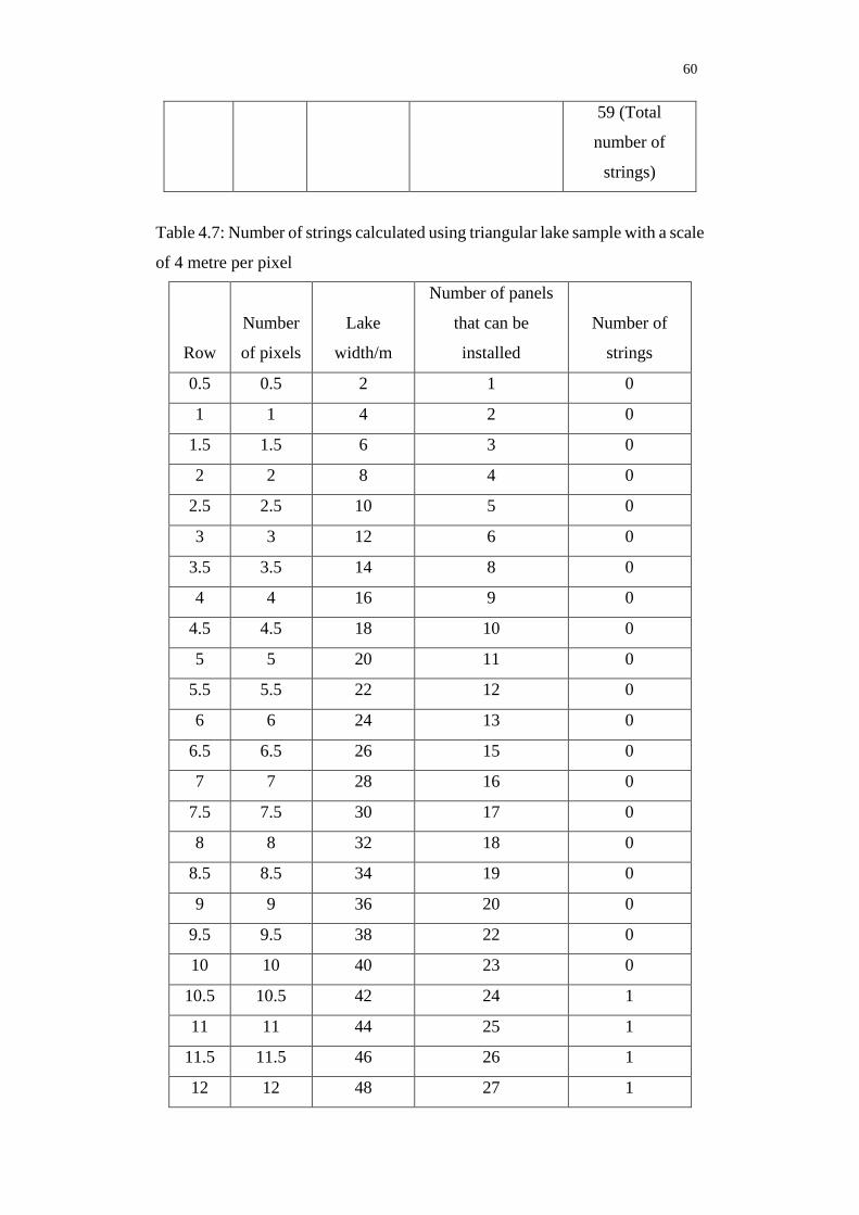
60

59 (Total

number of

strings)

Table 4.7: Number of strings calculated using triangular lake sample with a scale

of 4 metre per pixel

Row

Number

of pixels

Lake

width/m

Number of panels

that can be

installed

Number of

strings

0.5 0.5 2 1 0

1 1 4 2 0

1.5 1.5 6 3 0

2 2 8 4 0

2.5 2.5 10 5 0

3 3 12 6 0

3.5 3.5 14 8 0

4 4 16 9 0

4.5 4.5 18 10 0

5 5 20 11 0

5.5 5.5 22 12 0

6 6 24 13 0

6.5 6.5 26 15 0

7 7 28 16 0

7.5 7.5 30 17 0

8 8 32 18 0

8.5 8.5 34 19 0

9 9 36 20 0

9.5 9.5 38 22 0

10 10 40 23 0

10.5 10.5 42 24 1

11 11 44 25 1

11.5 11.5 46 26 1

12 12 48 27 1

61

12.5 12.5 50 29 1

13 13 52 30 1

13.5 13.5 54 31 1

14 14 56 32 1

14.5 14.5 58 33 1

15 15 60 34 1

15.5 15.5 62 36 1

16 16 64 37 1

16.5 16.5 66 38 1

17 17 68 39 1

17.5 17.5 70 40 1

18 18 72 41 1

18.5 18.5 74 43 1

19 19 76 44 1

19.5 19.5 78 45 1

20 20 80 46 1

20.5 20.5 82 47 1

21 21 84 48 2

21.5 21.5 86 49 2

22 22 88 51 2

22.5 22.5 90 52 2

23 23 92 53 2

23.5 23.5 94 54 2

24 24 96 55 2

24.5 24.5 98 56 2

25 25 100 58 2

25.5 25.5 102 59 2

26 26 104 60 2

26.5 26.5 106 61 2

27 27 108 62 2

27.5 27.5 110 63 2

28 28 112 65 2

62

28.5 28.5 114 66 2

29 29 116 67 2

29.5 29.5 118 68 2

30 30 120 69 2

30.5 30.5 122 70 2

31 31 124 72 3

31.5 31.5 126 73 3

32 32 128 74 3

32.5 32.5 130 75 3

33 33 132 76 3

33.5 33.5 134 77 3

34 34 136 79 3

34.5 34.5 138 80 3

35 35 140 81 3

35.5 35.5 142 82 3

36 36 144 83 3

36.5 36.5 146 84 3

37 37 148 86 3

37.5 37.5 150 87 3

38 38 152 88 3

38.5 38.5 154 89 3

39 39 156 90 3

39.5 39.5 158 91 3

40 40 160 93 3

40.5 40.5 162 94 3

41 41 164 95 3

41.5 41.5 166 96 4

42 42 168 97 4

42.5 42.5 170 98 4

43 43 172 99 4

43.5 43.5 174 101 4

44 44 176 102 4

63

44.5 44.5 178 103 4

45 45 180 104 4

45.5 45.5 182 105 4

46 46 184 106 4

46.5 46.5 186 108 4

47 47 188 109 4

47.5 47.5 190 110 4

48 48 192 111 4

48.5 48.5 194 112 4

49 49 196 113 4

49.5 49.5 198 115 4

50 50 200 116 4

50.5 50.5 202 117 4

51 51 204 118 4

51.5 51.5 206 119 4

52 52 208 120 5

52.5 52.5 210 122 5

53 53 212 123 5

53.5 53.5 214 124 5

54 54 216 125 5

54.5 54.5 218 126 5

55 55 220 127 5

55.5 55.5 222 129 5

56 56 224 130 5

56.5 56.5 226 131 5

57 57 228 132 5

57.5 57.5 230 133 5

58 58 232 134 5

58.5 58.5 234 136 5

59 59 236 137 5

59.5 59.5 238 138 5

60 60 240 139 5

64

293 (Total

number of

strings)

When 𝑚𝑒𝑡𝑟𝑒 𝑝𝑒𝑟 𝑝𝑖𝑥𝑒𝑙 = 2

𝑇𝑜𝑡𝑎𝑙 𝑛𝑢𝑚𝑏𝑒𝑟 𝑜𝑓 𝑠𝑡𝑟𝑖𝑛𝑔𝑠 = 59 (From Table 4.6)

𝑇𝑜𝑡𝑎𝑙 𝑛𝑢𝑚𝑏𝑒𝑟 𝑜𝑓 𝑝𝑎𝑛𝑒𝑙𝑠

= 𝑛𝑢𝑚𝑏𝑒𝑟 𝑜𝑓 𝑠𝑡𝑟𝑖𝑛𝑔𝑠 × 𝑛𝑢𝑚𝑏𝑒𝑟 𝑜𝑓 𝑝𝑎𝑛𝑒𝑙𝑠 𝑝𝑒𝑟 𝑠𝑡𝑟𝑖𝑛𝑔

= 59 × 24 = 1416

𝑃𝑉 𝑐𝑎𝑝𝑎𝑐𝑖𝑡𝑦 = 𝑛𝑢𝑚𝑏𝑒𝑟 𝑜𝑓 𝑝𝑎𝑛𝑒𝑙𝑠 × 𝑟𝑎𝑡𝑒𝑑 𝑝𝑜𝑤𝑒𝑟 𝑝𝑒𝑟 𝑝𝑎𝑛𝑒𝑙

= 1416 × 250 𝑊 = 0.354 𝑀𝑊

𝐴𝑛𝑛𝑢𝑎𝑙 𝑒𝑙𝑒𝑐𝑡𝑟𝑖𝑐𝑖𝑡𝑦 𝑦𝑖𝑒𝑙𝑑

= 𝑡𝑜𝑡𝑎𝑙 𝑛𝑢𝑚𝑏𝑒𝑟 𝑜𝑓 𝑝𝑎𝑛𝑒𝑙𝑠 × 𝑟𝑎𝑡𝑒𝑑 𝑝𝑜𝑤𝑒𝑟 𝑝𝑒𝑟 𝑝𝑎𝑛𝑒𝑙 ×

𝑝𝑒𝑎𝑘 𝑠𝑢𝑛 ℎ𝑜𝑢𝑟𝑠 𝑝𝑒𝑟 𝑦𝑒𝑎𝑟 × 𝑝𝑒𝑟𝑓𝑜𝑟𝑚𝑎𝑛𝑐𝑒 𝑟𝑎𝑡𝑖𝑜

= 1416 × 250 × 1600 × 0.8 = 453.12 𝑀𝑊ℎ

𝐿𝑎𝑘𝑒 𝑢𝑡𝑖𝑙𝑖𝑧𝑎𝑡𝑖𝑜𝑛 𝑟𝑎𝑡𝑒 =𝑡𝑜𝑡𝑎𝑙 𝑛𝑢𝑚𝑏𝑒𝑟 𝑜𝑓 𝑠𝑜𝑙𝑎𝑟 𝑝𝑎𝑛𝑒𝑙𝑠×𝑎𝑟𝑒𝑎 𝑜𝑓 𝑎 𝑠𝑜𝑙𝑎𝑟 𝑝𝑎𝑛𝑒𝑙

𝑙𝑎𝑘𝑒 𝑎𝑟𝑒𝑎=

1416×(1 𝑚 × 1.7 𝑚)

7200 𝑚2 = 33.43 %

When 𝑚𝑒𝑡𝑟𝑒 𝑝𝑒𝑟 𝑝𝑖𝑥𝑒𝑙 = 4

𝑇𝑜𝑡𝑎𝑙 𝑛𝑢𝑚𝑏𝑒𝑟 𝑜𝑓 𝑠𝑡𝑟𝑖𝑛𝑔𝑠 = 293 (From Table 4.7)

𝑇𝑜𝑡𝑎𝑙 𝑛𝑢𝑚𝑏𝑒𝑟 𝑜𝑓 𝑝𝑎𝑛𝑒𝑙𝑠

= 𝑛𝑢𝑚𝑏𝑒𝑟 𝑜𝑓 𝑠𝑡𝑟𝑖𝑛𝑔𝑠 × 𝑛𝑢𝑚𝑏𝑒𝑟 𝑜𝑓 𝑝𝑎𝑛𝑒𝑙𝑠 𝑝𝑒𝑟 𝑠𝑡𝑟𝑖𝑛𝑔

= 293 × 24 = 7032

𝑃𝑉 𝑐𝑎𝑝𝑎𝑐𝑖𝑡𝑦 = 𝑛𝑢𝑚𝑏𝑒𝑟 𝑜𝑓 𝑝𝑎𝑛𝑒𝑙𝑠 × 𝑟𝑎𝑡𝑒𝑑 𝑝𝑜𝑤𝑒𝑟 𝑝𝑒𝑟 𝑝𝑎𝑛𝑒𝑙

= 7032 × 250 𝑊 = 1.758 𝑀𝑊

𝐴𝑛𝑛𝑢𝑎𝑙 𝑒𝑙𝑒𝑐𝑡𝑟𝑖𝑐𝑖𝑡𝑦 𝑦𝑖𝑒𝑙𝑑

= 𝑡𝑜𝑡𝑎𝑙 𝑛𝑢𝑚𝑏𝑒𝑟 𝑜𝑓 𝑝𝑎𝑛𝑒𝑙𝑠 × 𝑟𝑎𝑡𝑒𝑑 𝑝𝑜𝑤𝑒𝑟 𝑝𝑒𝑟 𝑝𝑎𝑛𝑒𝑙 ×

𝑝𝑒𝑎𝑘 𝑠𝑢𝑛 ℎ𝑜𝑢𝑟𝑠 𝑝𝑒𝑟 𝑦𝑒𝑎𝑟 × 𝑝𝑒𝑟𝑓𝑜𝑟𝑚𝑎𝑛𝑐𝑒 𝑟𝑎𝑡𝑖𝑜

= 7032 × 250 × 1600 × 0.8 = 2250.24 𝑀𝑊ℎ

𝐿𝑎𝑘𝑒 𝑢𝑡𝑖𝑙𝑖𝑧𝑎𝑡𝑖𝑜𝑛 𝑟𝑎𝑡𝑒 =𝑡𝑜𝑡𝑎𝑙 𝑛𝑢𝑚𝑏𝑒𝑟 𝑜𝑓 𝑠𝑜𝑙𝑎𝑟 𝑝𝑎𝑛𝑒𝑙𝑠×𝑎𝑟𝑒𝑎 𝑜𝑓 𝑎 𝑠𝑜𝑙𝑎𝑟 𝑝𝑎𝑛𝑒𝑙

𝑙𝑎𝑘𝑒 𝑎𝑟𝑒𝑎=

7032×(1 𝑚 × 1.7 𝑚)

28800 𝑚2 = 41.51 %

65

4.4.3.3 Comparison of results obtained from two methods using triangular

lake sample

Table 4.8: Comparison of results using triangular lake sample with a scale of 2

metre per pixel

Python

algorithm

Manual calculation Percentage error

(%)

Lake area (𝑚2) 7320 7200 1.67

Number of strings

of panels

59 59 0

PV Capacity (MW) 0.354 0.354 0

Annual electricity

yield (MWh)

453.12 453.12 0

Lake utilization rate

(%)

32.89 33.43 1.62

Table 4.9: Comparison of results using triangular lake sample with a scale of 4

metre per pixel

Python

algorithm

Manual calculation Percentage error

(%)

Lake area (𝑚2) 29280 28800 1.67

Number of strings

of panels

296 293 1.02

PV Capacity (MW) 1.776 1.758 1.02

Annual electricity

yield (MWh)

2273.28 2250.24 1.02

Lake utilization rate

(%)

41.25 41.51 0.63

When the triangular lake sample is used as the input, it is found out that there is

an error in the lake area calculated. This is different from the rectangular and t-

shaped lake sample, which has no error. The error is due to the triangular lake

created because the triangle shape should have a smooth slanting line on the

66

hypotenuse side, as shown in Figure 4.29. However, the triangle shape created

will have a stair-step line, as shown in Figure 4.30. The image created is made

up of pixels that are the smallest unit displayed on the screen. For instance, when

a particular distance is equivalent to 0.8 pixels, 1 pixel will be used to represent

that distance. Therefore, the results obtained from the Python algorithm are

slightly higher than the actual results.

Two different scales are used to compare the percentage error, as

shown in Table 4.8 and Table 4.9. It is shown that the percentage error in the

calculation of PV capacity and annual electricity yield is higher for the case of

4 metres per pixel. When the zoom level is lower, the higher the value of metre

per pixel, and the number of solar panels installed on the lakes is also increased.

Meanwhile, the percentage error in the lake area and the lake utilisation rate are

lower when the zoom level is lower. This error is also applicable to the images

retrieved from Google Cloud Platform because all the Selangor lakes have an

irregular shape.

Figure 4.30: Triangular lake sample created

Figure 4.29: Normal triangle

67

CHAPTER 5

5 CONCLUSIONS AND RECOMMENDATIONS

5.1 Conclusions

The aim and objectives which are set at the beginning of the project are achieved.

A total of 57 lakes in Selangor have been captured by applying different zoom

levels. The lake area on the image is then identified using several image

processing techniques in Python. Some water areas that are not part of the lake

are also filtered out to obtain a better result. The area of each lake is also

calculated and recorded. The total lake area of the 57 lakes in Selangor is

25753279 𝑚2. The PV capacity and the first-year electricity yield for each lake

are also estimated individually and summed up, which are 1794.41 MW and

2296.84 GWh. Estimation of the PV capacity and the electricity yield is done

based on a floating solar system designed. The size of the solar panels, the rated

power per panel, the gaps between rows of solar panels are set to a value for the

calculation. The percentage of the lake area covered by the solar panels is also

set to be below 50 % to maintain the existing ecosystem inside all the lakes. The

verification of the results has been carried out by creating several known sizes

of the lake samples. The results obtained from the verification process are

satisfactory, and there might be an error of 1-2 % because the distance of the

lake will be rounded up into the nearest integer pixel. This error can be

minimized by maximizing the zoom level. It is also found out that the PV

capacity obtained is different when the orientations of solar panels are changed

according to the facing direction such as west, east, north and south. The south-

facing direction is chosen in this study because Malaysia is located in the

Northern hemisphere, so the south direction allows a maximum capture of

sunlight.

The results obtained, such as the PV capacity, have shown a positive

sign for the Malaysian government to develop and invest in floating solar farms.

It is another alternative solution to the ground-mounted solar system that can

increase renewable energy capacity and reduce the fossil fuel plants’ carbo

footprint. Although floating solar might have a higher capital cost than the

68

ground-mounted solar system, floating solar has its unique benefits, such as

eliminating land costs, higher efficiency of solar panels and lower operation and

management costs. Hence, it is recommended to involve floating solar as part

of the electricity generation in Malaysia.

5.2 Recommendations for future work

The floating solar in this project involves the lakes in Selangor state only. Hence,

it can be extended to other states in Malaysia to increase the sample size and get

a better insight. Besides, the number of solar panels per string is set to be a fixed

value of 24 in this study; thus, this value can be adjusted or customized

according to different lakes to optimize the lake area’s coverage. For instance,

different values for the number of panels per string, such as 18, 20, 22 and 24,

are used to calculate PV capacity. The value that results in the maximum PV

capacity is then selected.

The tilting angle of the solar panels can also be considered to obtain

higher accuracy of the results. For instance, the length of the solar panels is

calculated by using the Eq 5.1 below.

𝑙1 = 𝑙2 × 𝑐𝑜𝑠𝛽 (5.1)

where

𝑙1 = 𝑙𝑒𝑛𝑔𝑡ℎ 𝑜𝑓 𝑠𝑜𝑙𝑎𝑟 𝑝𝑎𝑛𝑒𝑙 𝑤𝑖𝑡ℎ 𝑡𝑖𝑙𝑡 𝑎𝑛𝑔𝑙𝑒, 𝑚

𝑙2 = 𝑙𝑒𝑛𝑔𝑡ℎ 𝑜𝑓𝑠𝑜𝑙𝑎𝑟 𝑝𝑎𝑛𝑒𝑙, 𝑚

𝛽 = 𝑡𝑖𝑙𝑡 𝑎𝑛𝑔𝑙𝑒 𝑜𝑓 𝑠𝑜𝑙𝑎𝑟 𝑝𝑎𝑛𝑒𝑙 𝑚𝑒𝑎𝑠𝑢𝑟𝑒𝑑 𝑓𝑟𝑜𝑚 𝑡ℎ𝑒 ℎ𝑜𝑟𝑖𝑧𝑜𝑛𝑡𝑎𝑙 𝑝𝑙𝑎𝑛𝑒, °

Moreover, the floating solar system on the sea can also be studied in the

future as Malaysia is surrounded by the sea. For floating solar farms on the sea,

more factors have to be considered, such as the strength of the supporting

structure to overcome the wave, the safety of the submarine cable and the

corrosion of the floating solar’s structure due to chemicals in seawater. Our

neighbouring country Singapore has built their first floating solar farm on the

sea. Hence, it is also possible to install floating solar panels on the sea in

Malaysia.

69

REFERENCES

Journals:

Abdullah, W.S., Osman, M., Ab Kadir, M.Z. and Verayiah, R., 2019. The

Potential and Status of Renewable Energy Development in Malaysia. Energies , .

Anon 2018. Riding the wave of solar energy: Why floating solar installations

are a positive step for energy generation.

Charles Lawrence, W., Lim, J., Won, C. and Ahn, H., 2018. Prediction Model

of Photovoltaic Module Temperature for Power Performance of Floating PVs.

Energies, 11, p.447.

Choi, Y.-K., Lee, N.-H. and Kim, K.-J., 2013. Empirical Research on the

efficiency of Floating PV systems compared with Overland PV Systems.

Dang Anh Thi, N., 2017. The global evolution of floating solar PV.

Davis, P. and Raianu, S., 2007. Computing areas using Green’s Theorem and a

Software Planimeter. Teaching Mathematics and Its Applications, 26, pp.103–

108.

Gamarra, C. and Ronk, J., 2019. Floating Solar: An Emerging Opportunity at

the Energy-Water Nexus.

Goswami, A., Sadhu, P., Goswami, U. and Sadhu, P., 2019. Floating Solar

Power Plant for Sustainable Development: A techno‐economic analysis.

Environmental Progress & Sustainable Energy, 38.

Kim, S.-H., Yoon, S.-J. and Choi, W., 2017. Design and Construction of 1 MW

Class Floating PV Generation Structural System Using FRP Members. Energies,

10, p.1142.

Kumar. J, C.R. and Majid, M.A., 2020. Renewable energy for sustainable

development in India: current status, future prospects, challenges, employment,

and investment opportunities. Energy, Sustainability and Society, [online] 10(1),

p.2.

Lee, Y.-G., Joo, H.-J. and Yoon, S.-J., 2014. Design and installation of floating

type photovoltaic energy generation system using FRP members. Solar Energy,

70

[online] 108, pp.13–27.

Manoj Kumar, N., Kanchikere, J. and Mallikarjun, P., 2018. Floatovoltaics:

Towards improved energy efficiency, land and water management.

International Journal of Civil Engineering and Technology, 9, pp.1089–1096.

Nordmann, T. and Clavadetscher, L., 2003. Understanding temperature effects

on PV system performance. 3rd World Conference onPhotovoltaic Energy

Conversion, 2003. Proceedings of, 3, pp.2243-2246 Vol.3.

Obaid, T., Hanon AlAsadi, A., Moslem, K. and Mohsen, 2016. A New Method

to Calculate an Irregular Area of a Lake using Image Processing Techniques.

International Journal of Computer Science and Mobile Computing, 51, pp.254–

260.

Puri, R. and Gupta, A., 2018. Contour, Shape & Color Detection using

OpenCV-Python.

Ranjan, P., Patel, J., Bhuva, J. and Gandhi, M., 2015. A Review on Solar

Photovoltaics and Roof Top Application of It. International Journal of

Computational Engineering Science, 2, pp.2394–2444.

Sahu, A., Yadav, N. and Sudhakar, K., 2016. Floating photovoltaic power plant:

A review. Renewable and Sustainable Energy Reviews, [online] 66, pp.815–824.

Srivastava, N., 2016. Canal Top Solar PV Plant in Gujarat: A Unique Nexus of

Energy, Land and Water. AksayUrja-MNRE, 10, pp.20–23.

Vaka, M., Walvekar, R., Rasheed, A.K. and Khalid, M., 2020. A review on

Malaysia’s solar energy pathway towards carbon-neutral Malaysia beyond

Covid’19 pandemic. Journal of Cleaner Production, [online] 273, p.122834.

TERI, 2019. Floating solar Phtovoltaic (FSPV): A Third Pillar to Solar PV

Sector?

World Bank Group, ESMAP and SERIS, 2019. Where Sun Meets Water:

Floating Solar Market Report. Washington, DC: World Bank.

71

Online resources:

Abhishek Shah, 2011. BIPV Solar Explained – Building Integrated

Photovoltaics Glass (Efficiency), Curtain Wall, Windows and Technology.

Retrieved from https://www.greenworldinvestor.com/2011/08/14/bipv-solar-

explained-building-integrated-photovoltaics-glass-efficiencycurtain-

wallwindows-and-technology/

Annabeth L., 2021. Malaysia’s solar capacity could cross 4GW in 2030, Fitch

estimates. Retrieved from https://www.businesstimes.com.sg/asean-

business/malaysias-solar-capacity-could-cross-4gw-in-2030-fitch-estimates

Ciel & Terre, n.d. Sungai Labu: 108 KWP. Retrieved from https://www.ciel-et-

terre.net/project/sungai-labu-108-kwp/

Djunisic, S., 2019. Hanergy covers building in China with 460 kW of BIPV

modules. Retrieved from https://renewablesnow.com/news/hanergy-covers-

building-in-china-with-460-kw-of-bipv-modules-661333/

Dricus, 2015. Floating Solar (PV) Systems: why they are taking off. Retrieved

from https://sinovoltaics.com/technology/floating-solar-pv-systems-why-they-

are-taking-off/

IRENA, 2020. Energy Profile (Malaysia). Retrieved from

https://www.irena.org/IRENADocuments/Statistical_Profiles/Asia/Malaysia_

Asia_RE_SP.pdf

IRENA, 2021. Renewable Capacity Statistics 2021. Retrieved from

https://www.irena.org/-

/media/Files/IRENA/Agency/Publication/2021/Apr/IRENA_RE_Capacity_Sta

tistics_2021.pdf

Mathis, W., 2020. Europe’s Largest Floating Solar Farm Underway in

Netherlands. Retrieved from https://www.bloomberg.com/news/articles/2020-

02-11/europe-s-largest-floating-solar-farm-underway-in-netherlands

Renewables Now, 2019. Singapore’s water agency to build 50-MWp floating

solar park. Retrieved from https://renewablesnow.com/news/singapores-water-

agency-to-build-50-mwp-floating-solar-park-

657314/#:~:text=June%2010%20(Renewables%20Now)%20%2D,2021%2C

%20PUB%20said%20last%20week.

Shift Energy Group, n.d. 5.5kW Ground Mount Solar Panel Installation in

Nanaimo BC. Retrieved from https://shiftenergygroup.com/project/5-5kw-

ground-mounted-solar-panel-system/

72

Simpleray, n.d. Are Solar Panels Bad For Your Roof? Retrieved from

https://www.simpleray.com/resources-and-informations/do-solar-panels-help-

protect-my-roof

Solarmo, 2020. 250W/30V Polycrystalline Solar Panel. Retrieved from

https://solarmo.com.my/product/250w30v-polycrystalline-solar-panel/

Solarvest, 2019. Floating Solar Farms. Retrieved from

https://solarvest.my/2019/07/29/floating-solar-farms/

Strong, S., 2016. Building Integrated Photovoltais (BIPV). Retrieved from

https://www.wbdg.org/resources/building-integrated-photovoltaics-bipv

Symbior Solar, n.d. Grand Opening of the Sig Solar Roof in Rayong – Biggest

Privately Financed Rooftop Solar Panel on the Fast Coast of Thailand.

Retrieved from https://symbiorsolar.com/news/rooftop-solar-panel-sig-

packaging-

plant/#:~:text=The%20SIG%20Rooftop%20Solar%20Panel,has%20now%20b

een%20officially%20opened.

Nelson, A., 2019. Floating solar projects gaining momentum. Retrieved from

https://ihsmarkit.com/research-analysis/floating-solar-projects-gaining-

momentum.html

KMB Design Group, 2019. Ground mounted photovoltaic systems vs rooftop:

which is right for you? Retrieved from

https://www.kmbdg.com/articles/ground-mounted-photovoltaic-systems/

Oceans of Energy, 2019. A world’s forst: offshore floating solar farm installed

at the Dutch North Sea. Retrieved from

https://oceansofenergy.blue/2019/12/11/a-worlds-first-offshore-floating-solar-

farm-installed-at-the-dutch-north-sea/

Rockikz, A., 2020. How to Detect Contours in Images using OpenCV in Python.

Retrieved from https://www.thepythoncode.com/article/contour-detection-

opencv-python

73

APPENDICES

APPENDIX A: Original Map Images

Original Map Image A-5.1: Batu Dam

Original Map Image A-2: Klang Gates Dam

74

Original Map Image A-3: Semenyih Dam

Original Map Image A-4: Sungai Langat Dam

75

Original Map Image A-5: Alam Impian Lake

Original Map Image A-6: Aman Lake

76

Original Map Image A-7: Ampang Hilir Lake

Original Map Image A-8: Bandar Bukit Raja Lake 1

77

Original Map Image A-9: Bandar Bukit Raja Lake 2

Original Map Image A-10: Bandar Tun Hussein Onn Lake

78

Original Map Image A-11: Bersatu Lake

Original Map Image A-12: Beruang Bbsa Lake

79

Original Map Image A-13: Biru Seri Kundang Lake

Original Map Image A-14: Cempaka Lake

80

Original Map Image A-15: Cyberjaya Lake 1

Original Map Image A-16: Cyberjaya Lake 2

81

Original Map Image A-17: D' Island Lake

Original Map Image A-18: D' Kayangan Lake

82

Original Map Image A-19: Fasa 1L Lake

Original Map Image A-20: Indah Mewah Lake

83

Original Map Image A-21: Kebun Serendah Lake

Original Map Image A-22: Kelana Lake

84

Original Map Image A-23: Kelana Jaya Lake

Original Map Image A-24: Kiambang Serendah Lake

85

Original Map Image A-25: Kota Kemuning Lake

Original Map Image A-26: Kota Puteri Lake

86

Original Map Image A-27: Metropolitan Kepong Lake

Original Map Image A-28: Millennium Lake

87

Original Map Image A-29: Pb Lake

Original Map Image A-30: Perdana Lake

88

Original Map Image A-31: Prima Lake

Original Map Image A-32: Putrajaya Lake Part 1

89

Original Map Image A-33: Putrajaya Lake Part 2

Original Map Image A-34: Putra Perdana Lake

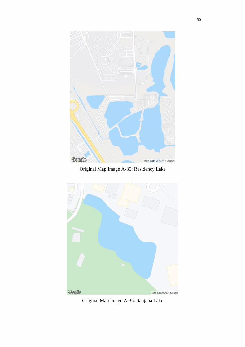
90

Original Map Image A-35: Residency Lake

Original Map Image A-36: Saujana Lake

91

Original Map Image A-37: Saujana Putra Lake

Original Map Image A-38: Seksyen 7 Lake

92

Original Map Image A-39: Semenyih Lake

Original Map Image A-40: Seri Aman Lake

93

Original Map Image A-41: Seri Serdang Lake

Original Map Image A-42: Serumpun Lake

94

Original Map Image A-43: Shah Alam Lake 1

Original Map Image A-44: Shah Alam Lake 2

95

Original Map Image A-45: Shah Alam Lake 3

Original Map Image A-46: Southlake Residence Lake

96

Original Map Image A-47: Sri Murni Lake

Original Map Image A-48: Sri Rampai Lake

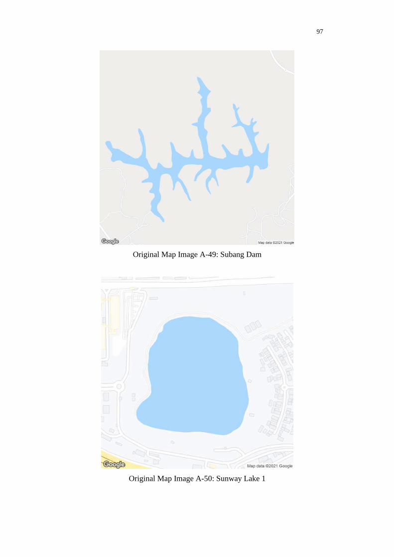
97

Original Map Image A-49: Subang Dam

Original Map Image A-50: Sunway Lake 1

98

Original Map Image A-51: Sunway Lake 2

Original Map Image A-52: Sunway Serene Lake

99

Original Map Image A-53: Taman Dengkil Jaya Lake

Original Map Image A-54: Taman Subang Ria Lake

100

Original Map Image A-55: Teratai Lake 1

Original Map Image A-56: Teratai Lake 2

101

Original Map Image A-57: The Mines Lake

Original Map Image A-58: Titiwangsa Lake

102

APPENDIX B: Final Processed Images

Final Processed Image B-5.2: Batu Dam

Final Processed Image B-2: Klang Gates Dam

103

Final Processed Image B-3: Semenyih Dam

Final Processed Image B-4: Sungai Langat Dam

104

Final Processed Image B-5: Alam Impian Lake

Final Processed Image B-6: Aman Lake

105

Final Processed Image B-7: Ampang Hilir Lake

Final Processed Image B-8: Bandar Bukit Raja Lake 1

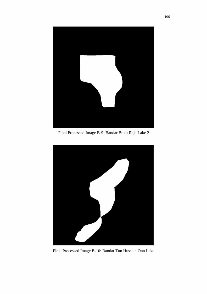
106

Final Processed Image B-9: Bandar Bukit Raja Lake 2

Final Processed Image B-10: Bandar Tun Hussein Onn Lake

107

Final Processed Image B-11: Bersatu Lake

Final Processed Image B-12: Beruang Bbsa Lake

108

Final Processed Image B-13: Biru Seri Kundang Lake

Final Processed Image B-14: Cempaka Lake

109

Final Processed Image B-15: Cyberjaya Lake 1

Final Processed Image B-16: Cyberjaya Lake 2

110

Final Processed Image B-17: D' Island Lake

Final Processed Image B-18: D' Kayangan Lake

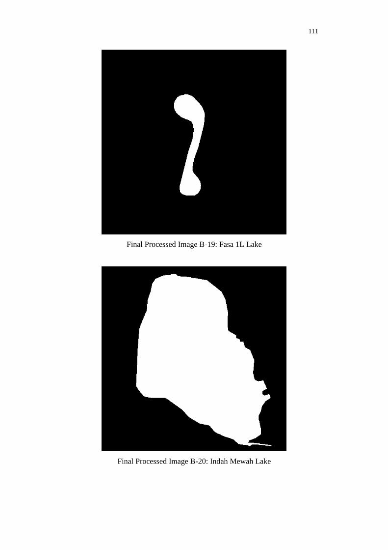
111

Final Processed Image B-19: Fasa 1L Lake

Final Processed Image B-20: Indah Mewah Lake

112

Final Processed Image B-21: Kebun Serendah Lake

Final Processed Image B-22: Kelana Lake

113

Final Processed Image B-23: Kelana Jaya Lake

Final Processed Image B-24: Kiambang Serendah Lake

114

Final Processed Image B-25: Kota Kemuning Lake

Final Processed Image B-26: Kota Puteri Lake

115

Final Processed Image B-27: Metropolitan Kepong Lake

Final Processed Image B-28: Millennium Lake

116

Final Processed Image B-29: Pb Lake

Final Processed Image B-30: Perdana Lake

117

Final Processed Image B-31: Prima Lake

Final Processed Image B-32: Putrajaya Lake Part 1

118

Final Processed Image B-33: Putrajaya Lake Part 2

Final Processed Image B-34: Putra Perdana Lake

119

Final Processed Image B-35: Residency Lake

Final Processed Image B-36: Saujana Lake

120

Final Processed Image B-37: Saujana Putra Lake

Final Processed Image B-38: Seksyen 7 Lake

121

Final Processed Image B-39: Semenyih Lake

Final Processed Image B-40: Seri Aman Lake

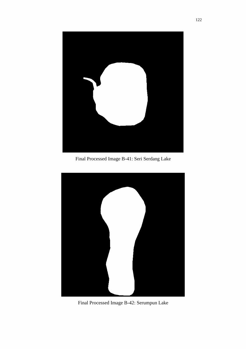
122

Final Processed Image B-41: Seri Serdang Lake

Final Processed Image B-42: Serumpun Lake

123

Final Processed Image B-43: Shah Alam Lake 1

Final Processed Image B-44: Shah Alam Lake 2

124

Final Processed Image B-45: Shah Alam Lake 3

Final Processed Image B-46: Southlake Residence Lake

125

Final Processed Image B-47: Sri Murni Lake

Final Processed Image B-48: Sri Rampai Lake

126

Final Processed Image B-49: Subang Dam

Final Processed Image B-50: Sunway Lake 1

127

Final Processed Image B-51: Sunway Lake 2

Final Processed Image B-52: Sunway Serene Lake

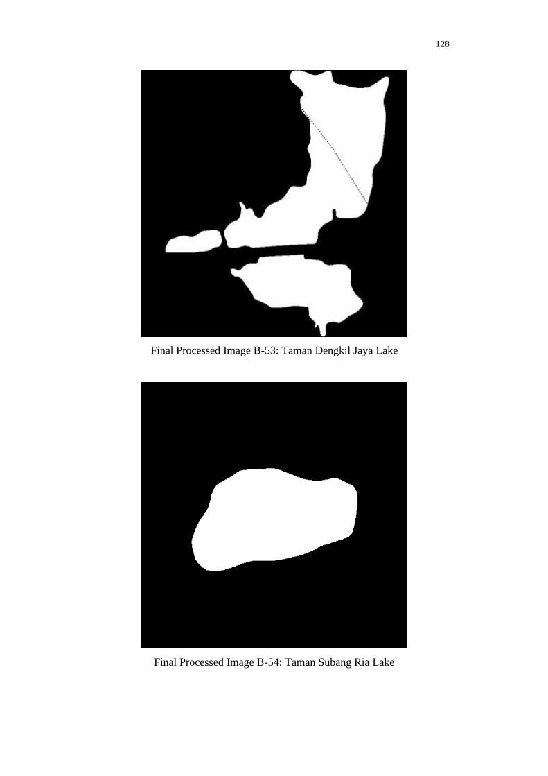
128

Final Processed Image B-53: Taman Dengkil Jaya Lake

Final Processed Image B-54: Taman Subang Ria Lake

129

Final Processed Image B-55: Teratai Lake 1

Final Processed Image B-56: Teratai Lake 2

130

Final Processed Image B-57: The Mines Lake

Final Processed Image B-58: Titiwangsa Lake

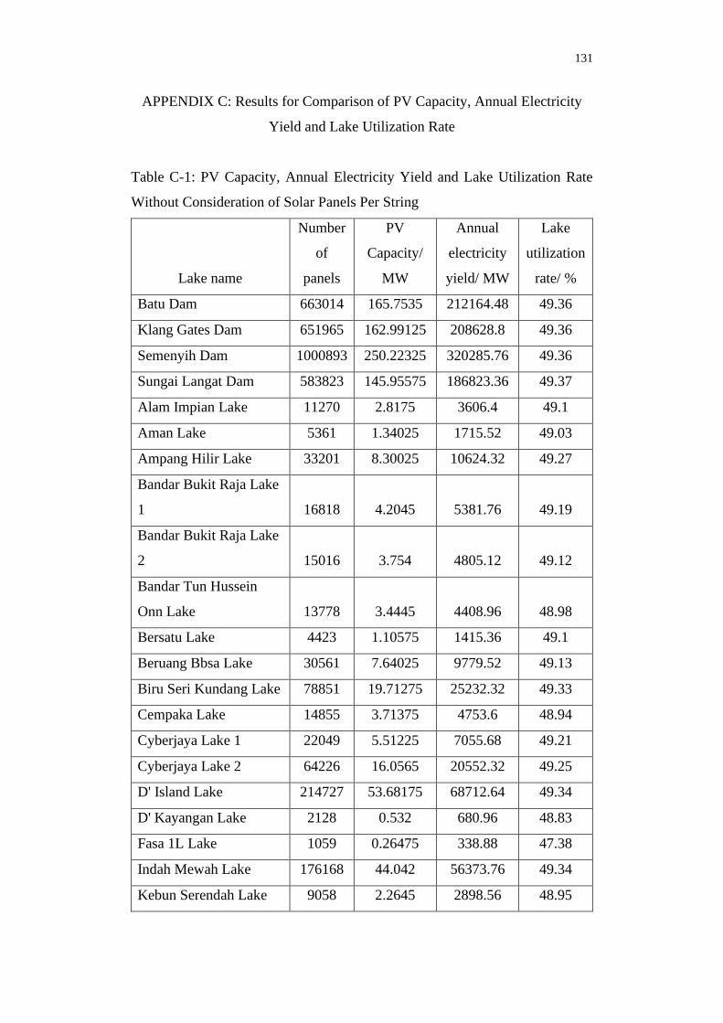
131

APPENDIX C: Results for Comparison of PV Capacity, Annual Electricity

Yield and Lake Utilization Rate

Table C-1: PV Capacity, Annual Electricity Yield and Lake Utilization Rate

Without Consideration of Solar Panels Per String

Lake name

Number

of

panels

PV

Capacity/

MW

Annual

electricity

yield/ MW

Lake

utilization

rate/ %

Batu Dam 663014 165.7535 212164.48 49.36

Klang Gates Dam 651965 162.99125 208628.8 49.36

Semenyih Dam 1000893 250.22325 320285.76 49.36

Sungai Langat Dam 583823 145.95575 186823.36 49.37

Alam Impian Lake 11270 2.8175 3606.4 49.1

Aman Lake 5361 1.34025 1715.52 49.03

Ampang Hilir Lake 33201 8.30025 10624.32 49.27

Bandar Bukit Raja Lake

1 16818 4.2045 5381.76 49.19

Bandar Bukit Raja Lake

2 15016 3.754 4805.12 49.12

Bandar Tun Hussein

Onn Lake 13778 3.4445 4408.96 48.98

Bersatu Lake 4423 1.10575 1415.36 49.1

Beruang Bbsa Lake 30561 7.64025 9779.52 49.13

Biru Seri Kundang Lake 78851 19.71275 25232.32 49.33

Cempaka Lake 14855 3.71375 4753.6 48.94

Cyberjaya Lake 1 22049 5.51225 7055.68 49.21

Cyberjaya Lake 2 64226 16.0565 20552.32 49.25

D' Island Lake 214727 53.68175 68712.64 49.34

D' Kayangan Lake 2128 0.532 680.96 48.83

Fasa 1L Lake 1059 0.26475 338.88 47.38

Indah Mewah Lake 176168 44.042 56373.76 49.34

Kebun Serendah Lake 9058 2.2645 2898.56 48.95

132

Kelana Lake 18516 4.629 5925.12 49.16

Kelana Jaya Lake 21380 5.345 6841.6 49.16

Kiambang Serendah

Lake 69910 17.4775 22371.2 49.3

Kota Kemuning Lake 20279 5.06975 6489.28 49.19

Kota Puteri Lake 21200 5.3 6784 49.18

Metropolitan Kepong

Lake 130643 32.66075 41805.76 49.33

Millennium Lake 52547 13.13675 16815.04 49.24

Pb Lake 18721 4.68025 5990.72 49.16

Perdana Lake 10749 2.68725 3439.68 48.77

Prima Lake 329990 82.4975 105596.8 49.34

Putrajaya Lake Part 1 745271 186.31775 238486.72 49.36

Putrajaya Lake Part 2 424705 106.17625 135905.6 49.31

Putra Perdana Lake 547316 136.829 175141.12 49.39

Residency Lake 226067 56.51675 72341.44 49.31

Saujana Lake 4725 1.18125 1512 48.85

Saujana Putra Lake 238878 59.7195 76440.96 49.36

Seksyen 7 Lake 25923 6.48075 8295.36 49.21

Semenyih Lake 15453 3.86325 4944.96 49.27

Seri Aman Lake 41134 10.2835 13162.88 49.25

Seri Serdang Lake 4979 1.24475 1593.28 48.93

Serumpun Lake 1332 0.333 426.24 48.24

Shah Alam Lake 1 25201 6.30025 8064.32 49.15

Shah Alam Lake 2 6529 1.63225 2089.28 48.92

Shah Alam Lake 3 8849 2.21225 2831.68 49.21

Southlake residence

Lake 19282 4.8205 6170.24 49.07

Sri Murni Lake 49276 12.319 15768.32 49.22

Sri Rampai Lake 6221 1.55525 1990.72 49.02

Subang Dam 253448 63.362 81103.36 49.3

Sunway Lake 1 28551 7.13775 9136.32 49.22

133

Sunway Lake 2 8615 2.15375 2756.8 49.08

Sunway Serene Lake 12412 3.103 3971.84 49.05

Taman Dengkil Jaya

Lake 48293 12.07325 15453.76 49.22

Taman Subang Ria Lake 17887 4.47175 5723.84 49.28

Teratai Lake 1 75432 18.858 24138.24 49.28

Teratai Lake 2 80155 20.03875 25649.6 49.28

The Mines Lake 209580 52.395 67065.6 49.3

Titiwangsa Lake 40546 10.1365 12974.72 49.25

7473239

(Total)

1868.30975

(Total)

2391436.48

(Total)

49.14

(Average)

Table C-2: PV capacity, annual electricity yield and lake utilization rate for

arrangement of solar panels from direction of south to north

Lake name

Number

of strings

PV

Capacity/

MW

Annual

electricity

yield/ MW

Lake

utilization

rate/ %

Batu Dam 26959 161.754 207045.12 48.17

Klang Gates Dam 26355 158.13 202406.4 47.89

Semenyih Dam 40565 243.39 311539.2 48.01

Sungai Langat Dam 23839 143.034 183083.52 48.39

Alam Impian Lake 405 2.43 3110.4 42.35

Aman Lake 194 1.164 1489.92 42.59

Ampang Hilir Lake 1285 7.71 9868.8 45.77

Bandar Bukit Raja Lake

1 603 3.618 4631.04 42.33

Bandar Bukit Raja Lake

2 561 3.366 4308.48 44.04

Bandar Tun Hussein

Onn Lake 460 2.76 3532.8 39.25

Bersatu Lake 155 0.93 1190.4 41.29

134

Beruang Bbsa Lake 1094 6.564 8401.92 42.21

Biru Seri Kundang

Lake 3120 18.72 23961.6 46.84

Cempaka Lake 501 3.006 3847.68 39.61

Cyberjaya Lake 1 843 5.058 6474.24 45.15

Cyberjaya Lake 2 2507 15.042 19253.76 46.13

D' Island Lake 8616 51.696 66170.88 47.51

D' Kayangan Lake 68 0.408 522.24 37.45

Fasa 1L Lake 9 0.054 69.12 9.66

Indah Mewah Lake 7084 42.504 54405.12 47.62

Kebun Serendah Lake 305 1.83 2342.4 39.56

Kelana Lake 683 4.098 5245.44 43.52

Kelana Jaya Lake 776 4.656 5959.68 42.83

Kiambang Serendah

Lake 2770 16.62 21273.6 46.88

Kota Kemuning Lake 752 4.512 5775.36 43.77

Kota Puteri Lake 791 4.746 6074.88 44.04

Metropolitan Kepong

Lake 5208 31.248 39997.44 47.2

Millennium Lake 2022 12.132 15528.96 45.48

Pb Lake 690 4.14 5299.2 43.49

Perdana Lake 304 1.824 2334.72 33.12

Prima Lake 13297 79.782 102120.96 47.72

Putrajaya Lake Part 1 30181 181.086 231790.08 47.98

Putrajaya Lake Part 2 16854 101.124 129438.72 46.96

Putra Perdana Lake 22425 134.55 172224 48.57

Residency Lake 8912 53.472 68444.16 46.65

Saujana Lake 147 0.882 1128.96 36.48

Saujana Putra Lake 9744 58.464 74833.92 48.33

Seksyen 7 Lake 984 5.904 7557.12 44.83

Semenyih Lake 585 3.51 4492.8 44.76

Seri Aman Lake 1607 9.642 12341.76 46.18

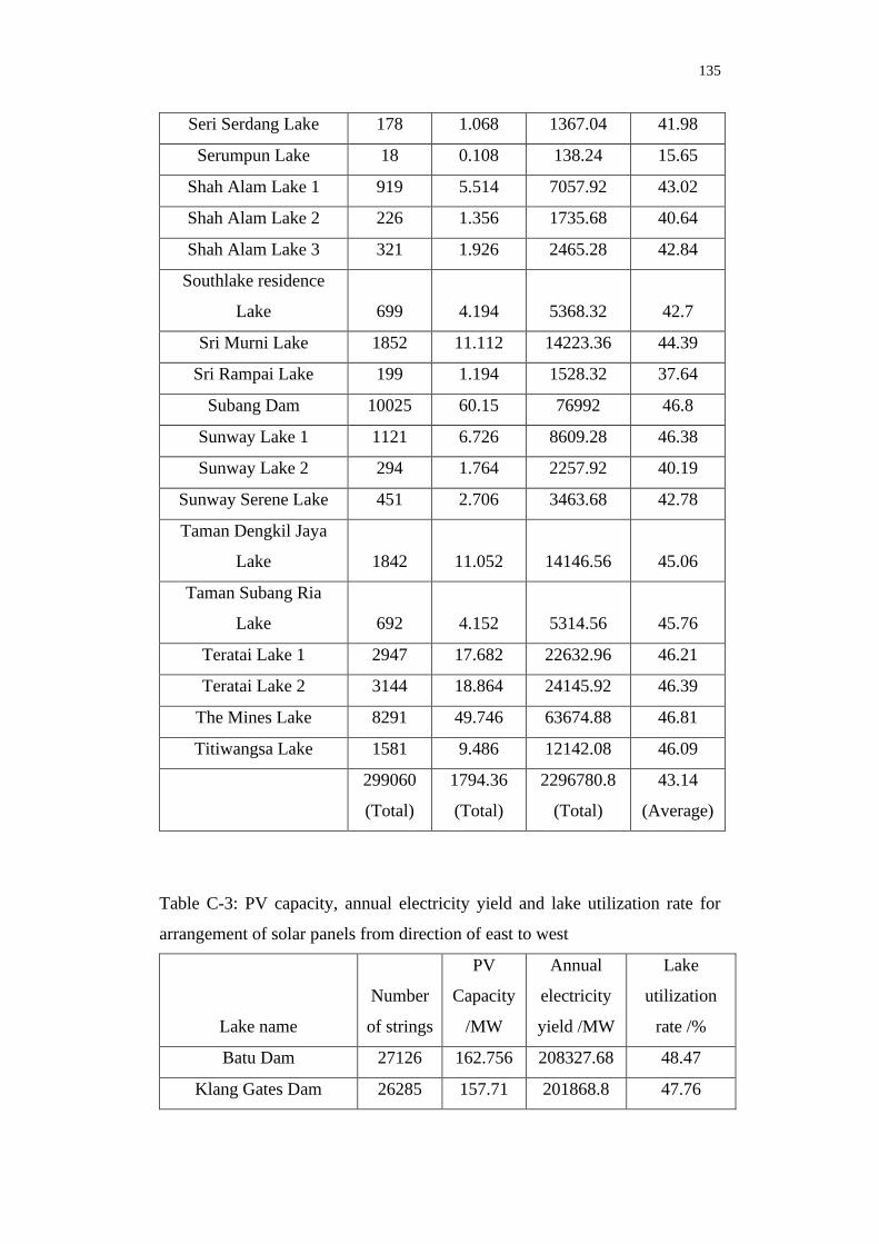
135

Seri Serdang Lake 178 1.068 1367.04 41.98

Serumpun Lake 18 0.108 138.24 15.65

Shah Alam Lake 1 919 5.514 7057.92 43.02

Shah Alam Lake 2 226 1.356 1735.68 40.64

Shah Alam Lake 3 321 1.926 2465.28 42.84

Southlake residence

Lake 699 4.194 5368.32 42.7

Sri Murni Lake 1852 11.112 14223.36 44.39

Sri Rampai Lake 199 1.194 1528.32 37.64

Subang Dam 10025 60.15 76992 46.8

Sunway Lake 1 1121 6.726 8609.28 46.38

Sunway Lake 2 294 1.764 2257.92 40.19

Sunway Serene Lake 451 2.706 3463.68 42.78

Taman Dengkil Jaya

Lake 1842 11.052 14146.56 45.06

Taman Subang Ria

Lake 692 4.152 5314.56 45.76

Teratai Lake 1 2947 17.682 22632.96 46.21

Teratai Lake 2 3144 18.864 24145.92 46.39

The Mines Lake 8291 49.746 63674.88 46.81

Titiwangsa Lake 1581 9.486 12142.08 46.09

299060

(Total)

1794.36

(Total)

2296780.8

(Total)

43.14

(Average)

Table C-3: PV capacity, annual electricity yield and lake utilization rate for

arrangement of solar panels from direction of east to west

Lake name

Number

of strings

PV

Capacity

/MW

Annual

electricity

yield /MW

Lake

utilization

rate /%

Batu Dam 27126 162.756 208327.68 48.47

Klang Gates Dam 26285 157.71 201868.8 47.76

136

Semenyih Dam 40615 243.69 311923.2 48.07

Sungai Langat Dam 23708 142.248 182077.44 48.12

Alam Impian Lake 385 2.31 2956.8 40.26

Aman Lake 164 0.984 1259.52 36

Ampang Hilir Lake 1264 7.584 9707.52 45.02

Bandar Bukit Raja Lake

1 627 3.762 4815.36 44.01

Bandar Bukit Raja Lake

2 562 3.372 4316.16 44.12

Bandar Tun Hussein Onn

Lake 497 2.982 3816.96 42.41

Bersatu Lake 127 0.762 975.36 33.84

Beruang Bbsa Lake 1191 7.146 9146.88 45.95

Biru Seri Kundang Lake 3123 18.738 23984.64 46.89

Cempaka Lake 547 3.282 4200.96 43.25

Cyberjaya Lake 1 835 5.01 6412.8 44.72

Cyberjaya Lake 2 2544 15.264 19537.92 46.82

D' Island Lake 8713 52.278 66915.84 48.05

D' Kayangan Lake 49 0.294 376.32 26.99

Fasa 1L Lake 34 0.204 261.12 36.51

Indah Mewah Lake 7139 42.834 54827.52 47.99

Kebun Serendah Lake 311 1.866 2388.48 40.34

Kelana Lake 691 4.146 5306.88 44.03

Kelana Jaya Lake 817 4.902 6274.56 45.09

Kiambang Serendah

Lake 2794 16.764 21457.92 47.29

Kota Kemuning Lake 722 4.332 5544.96 42.03

Kota Puteri Lake 795 4.77 6105.6 44.26

Metropolitan Kepong

Lake 5273 31.638 40496.64 47.79

Millennium Lake 2010 12.06 15436.8 45.21

Pb Lake 675 4.05 5184 42.54

137

Perdana Lake 377 2.262 2895.36 41.07

Prima Lake 13465 80.79 103411.2 48.32

Putrajaya Lake Part 1 30052 180.312 230799.36 47.77

Putrajaya Lake Part 2 17082 102.492 131189.76 47.6

Putra Perdana Lake 22324 133.944 171448.32 48.35

Residency Lake 9122 54.732 70056.96 47.75

Saujana Lake 146 0.876 1121.28 36.23

Saujana Putra Lake 9581 57.486 73582.08 47.52

Seksyen 7 Lake 1001 6.006 7687.68 45.61

Semenyih Lake 443 2.658 3402.24 33.9

Seri Aman Lake 1591 9.546 12218.88 45.72

Seri Serdang Lake 169 1.014 1297.92 39.86

Serumpun Lake 48 0.288 368.64 41.72

Shah Alam Lake 1 944 5.664 7249.92 44.19

Shah Alam Lake 2 192 1.152 1474.56 34.53

Shah Alam Lake 3 319 1.914 2449.92 42.58

Southlake residence

Lake 749 4.494 5752.32 45.75

Sri Murni Lake 1952 11.712 14991.36 46.79

Sri Rampai Lake 216 1.296 1658.88 40.85

Subang Dam 9964 59.784 76523.52 46.52

Sunway Lake 1 1106 6.636 8494.08 45.76

Sunway Lake 2 288 1.728 2211.84 39.37

Sunway Serene Lake 468 2.808 3594.24 44.39

Taman Dengkil Jaya

Lake 1875 11.25 14400 45.86

Taman Subang Ria Lake 635 3.81 4876.8 41.99

Teratai Lake 1 3034 18.204 23301.12 47.57

Teratai Lake 2 3167 19.002 24322.56 46.73

The Mines Lake 8560 51.36 64740.8 48.33

Titiwangsa Lake 1524 9.144 11704.32 44.43

138

300017

(Total)

1800.102

(Total)

2303130.56

(Total)

43.81

(Average)

Table C-4: PV capacity, annual electricity yield and lake utilization rate for

arrangement of solar panels from direction of west to east

Lake name

Number

of strings

PV

Capacity

/MW

Annual

electricity

yield /MW

Lake

utilization

rate /%

Batu Dam 27126 162.756 208327.68 48.47

Klang Gates Dam 26281 157.686 201838.08 47.75

Semenyih Dam 40624 243.744 311992.32 48.08

Sungai Langat Dam 23703 142.218 182039.04 48.11

Alam Impian Lake 386 2.316 2964.48 40.36

Aman Lake 162 0.972 1244.16 35.56

Ampang Hilir Lake 1264 7.584 9707.52 45.02

Bandar Bukit Raja Lake

1 626 3.756 4807.68 43.94

Bandar Bukit Raja Lake

2 562 3.372 4316.16 44.12

Bandar Tun Hussein Onn

Lake 496 2.976 3809.28 42.32

Bersatu Lake 129 0.774 990.72 34.37

Beruang Bbsa Lake 1188 7.128 9123.84 45.84

Biru Seri Kundang Lake 3120 18.72 23961.6 46.84

Cempaka Lake 547 3.282 4200.96 43.25

Cyberjaya Lake 1 832 4.992 6389.76 44.56

Cyberjaya Lake 2 2548 15.288 19568.64 46.89

D' Island Lake 8710 52.26 66892.8 48.03

D' Kayangan Lake 50 0.3 384 27.54

Fasa 1L Lake 34 0.204 261.12 36.51

Indah Mewah Lake 7141 42.846 54842.88 48

Kebun Serendah Lake 312 1.872 2396.16 40.47

139

Kelana Lake 689 4.134 5291.52 43.9

Kelana Jaya Lake 816 4.896 6266.88 45.03

Kiambang Serendah

Lake 2794 16.764 21457.92 47.29

Kota Kemuning Lake 718 4.308 5514.24 41.8

Kota Puteri Lake 795 4.77 6105.6 44.26

Metropolitan Kepong

Lake 5275 31.65 40512 47.8

Millennium Lake 2009 12.054 15429.12 45.18

Pb Lake 675 4.05 5184 42.54

Perdana Lake 377 2.262 2895.36 41.07

Prima Lake 13464 80.784 103403.52 48.32

Putrajaya Lake Part 1 30049 180.294 230776.32 47.77

Putrajaya Lake Part 2 17083 102.498 131197.44 47.6

Putra Perdana Lake 22322 133.932 171432.96 48.34

Residency Lake 9128 54.768 70103.04 47.78

Saujana Lake 147 0.882 1128.96 36.48

Saujana Putra Lake 9577 57.462 73551.36 47.5

Seksyen 7 Lake 995 5.97 7641.6 45.33

Semenyih Lake 450 2.7 3456 34.43

Seri Aman Lake 1591 9.546 12218.88 45.72

Seri Serdang Lake 169 1.014 1297.92 39.86

Serumpun Lake 46 0.276 353.28 39.98

Shah Alam Lake 1 946 5.676 7265.28 44.28

Shah Alam Lake 2 192 1.152 1474.56 34.53

Shah Alam Lake 3 318 1.908 2442.24 42.44

Southlake residence

Lake 748 4.488 5744.64 45.69

Sri Murni Lake 1953 11.718 14999.04 46.81

Sri Rampai Lake 214 1.284 1643.52 40.47

Subang Dam 9975 59.85 76608 46.57

Sunway Lake 1 1106 6.636 8494.08 45.76

140

Sunway Lake 2 289 1.734 2219.52 39.51

Sunway Serene Lake 470 2.82 3609.6 44.58

Taman Dengkil Jaya

Lake 1876 11.256 14407.68 45.89

Taman Subang Ria Lake 635 3.81 4876.8 41.99

Teratai Lake 1 3038 18.228 23331.84 47.63

Teratai Lake 2 3164 18.984 24299.52 46.69

The Mines Lake 8560 51.36 64740.8 48.33

Titiwangsa Lake 1525 9.15 11712 44.46

300019

(Total)

1800.114

(Total)

2303145.92

(Total)

43.79

(Average)

141

APPENDIX D: Floating solar system design

Floating solar system design D-1: Specifications of solar panels in this study

(Solarmo, 2020)

Floating solar system design D-2: Floating system (Lee, Joo and Yoon, 2014)

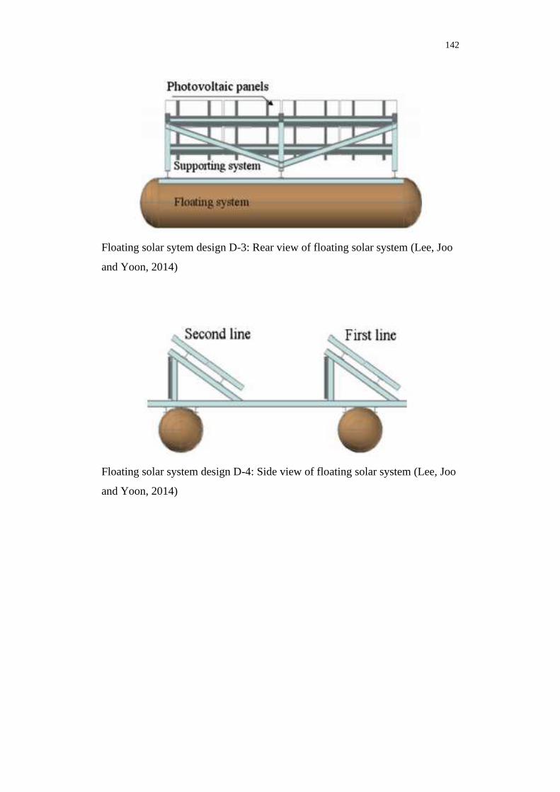
142

Floating solar sytem design D-3: Rear view of floating solar system (Lee, Joo

and Yoon, 2014)

Floating solar system design D-4: Side view of floating solar system (Lee, Joo

and Yoon, 2014)