Study of impact demagnetization at Mars using Monte …rcoe/eart290C/Additional Papers/Lillis... · Click Here for Full Article Study of impact demagnetization at Mars using Monte

ClickHere

for

FullArticle

Study of impact demagnetization at Mars using Monte Carlomodeling and multiple altitude data

Robert J. Lillis,1 Michael E. Purucker,2 Jasper S. Halekas,1 Karin L. Louzada,3,4

Sarah T. Stewart‐Mukhopadhyay,3 Michael Manga,5 and Herbert V. Frey2

Received 4 December 2009; revised 10 February 2010; accepted 12 March 2010; published 17 July 2010.

[1] The magnetic field signatures of large demagnetized impact basins on Mars offer aunique opportunity to study the magnetic properties of the crust and the processes of basinformation and impact shock demagnetization. We present a framework for determiningthe effects on such signatures due to the dominant direction, strength, thickness, andvertical and horizontal coherence wavelengths of the surrounding crustal magnetization, aswell as the demagnetization radius and the width of the demagnetization gradient zonecaused by impact shock. By comparing model results with observed magnetic field profilesat 185 km and 400 km over the five largest apparently demagnetized impact structures, wefind that (1) the dominant lateral size of coherently magnetized regions of crust falls inthe range ∼325 km to 600 km, (2) the magnetic field observed over a circulardemagnetized region is such that clear demagnetization signatures should only be visiblein magnetic field maps at 185 km and 400 km altitude for demagnetization diameterslarger than ∼600 km and ∼1000 km, respectively, (3) demagnetization radii can bemeaningfully constrained despite relatively poor constraints on associated demagnetizationgradient zone widths, (4) the ratio of demagnetization diameter to the outer topographicring diameter is close to 0.8 for the Isidis, Hellas, Argyre, and Utopia basins, suggestingthat similar basin‐forming and shock demagnetization processes occurred in each ofthese four ancient impacts, and (5) if used in conjunction with impact simulations, suchmodeling may lead to improved constraints on peak pressure contours and impact energiesfor these basins.

Citation: Lillis, R. J., M. E. Purucker, J. S. Halekas, K. L. Louzada, S. T. Stewart‐Mukhopadhyay, M. Manga, and H. V. Frey(2010), Study of impact demagnetization at Mars using Monte Carlo modeling and multiple altitude data, J. Geophys. Res., 115,E07007, doi:10.1029/2009JE003556.

1. Introduction

[2] Mars today does not possess a global dynamo‐drivenmagnetic field but, from evidence of strong crustal magne-tization, such a field is almost certain to have existed in theplanet’s early history [Acuña et al., 1999]. The dynamo isthought to have started immediately following accretion/differentiation [Williams and Nimmo, 2004] prior to theformation of most of the planetary crust, >4.3 Ga ago. Thishypothesis is consistent with recent lunar sample andmeteoritic work implying that dynamos within planetesimals

were common in the early solar system [Garrick‐Bethellet al., 2009; Weiss et al., 2008, 2009].[3] Large impacts on Mars, such as those responsible for

the Hellas and Argyre impact basins, alter the magnetizationof the entire depth of crust over a geographic area compa-rable to the final size of the impact basin [Hood et al., 2003;Shahnas and Arkani‐Hamed, 2007]. Excavation can removemagnetized material and shock heating causes thermaldemagnetization within the basin [Mohit and Arkani‐Hamed,2004]. As the crust cools immediately following the impact,the melt sheet and any other crustal minerals heated abovetheir Curie point can acquire a new thermoremanent magne-tization (TRM) with a magnitude proportional to the strengthof the local ambient magnetic field and the capability of therock to carry thermoremanence. In addition, shock from theimpact can add or remove net magnetization, dependingon this local magnetic field and prior magnetization state ofthe crust. Unmagnetized materials can be magnetized in anexternal magnetic field through shock remanent magneti-zation (SRM) and existing magnetization can be reduced orerased if the minerals are shocked in an ambient field tooweak to induce a sufficient SRM [Cisowski and Fuller,

1Space Sciences Laboratory, University of California, Berkeley,California, USA.

2Planetary Geodynamics Laboratory, NASA Goddard Space FlightCenter, Greenbelt, Maryland, USA.

3Department of Earth and Planetary Sciences, Harvard University,Cambridge, Massachusetts, USA.

4Netherlands Office for Science and Technology, Royal NetherlandsEmbassy, Washington, D. C., USA.

5Department of Earth and Planetary Sciences, University of California,Berkeley, California, USA.

Copyright 2010 by the American Geophysical Union.0148‐0227/10/2009JE003556

JOURNAL OF GEOPHYSICAL RESEARCH, VOL. 115, E07007, doi:10.1029/2009JE003556, 2010

E07007 1 of 22

http://dx.doi.org/10.1029/2009JE003556

1978, Gattacceca et al., 2008]. Brecciation and fluid cir-culation can combine to produce post‐impact hydrothermalsystems which can lead to the acquisition by crustal rocks ofchemical remanent magnetization (CRM), the strength ofwhich is controlled primarily by oxygen fugacity and cool-ing speed [Grant, 1985]. It is important to note that essen-tially all magnetization in Martian impact structures is TRM,SRM or CRM, comprising what is commonly referred to asnatural remanent magnetization (NRM). This is in contrastto the case of terrestrial impact structures where a substantialcomponent of magnetization induced by the geomagneticfield can account for anywhere from ∼5% to >90% of totalmagnetization [Ugalde et al., 2005]. Mars’ lack of a globalmagnetic field, and hence inducedmagnetization, thus removesa substantial complication from the interpretation of impactbasin magnetic signatures.[4] It is also important to note that short‐wavelength, strong

NRM within an impact structure (compared with outside thestructure), as is observed for some terrestrial impact structuressuch as Chicxulub [Rebolledo‐Vieyra, 2001] and Vredefort[Carporzen et al., 2005], results in magnetic field lowsmeasured at high altitudes because magnetic fields fromshorter‐wavelength magnetization decay more rapidly thanlonger‐wavelength magnetization. Indeed at Vredefort,

magnetic lows are seen at aeromagnetic altitudes of hundredsof meters because the magnetization coherence length is assmall as centimeters [Carporzen et al., 2005].[5] For any of the iron‐bearing minerals likely responsible

for Mars’ remanent magnetism, shock demagnetizationoccurs out to larger distances from the impact point comparedwith thermal demagnetization [e.g.,Mohit and Arkani‐Hamed,2004]. The very weak crustal magnetic fields measured at100 km–400 km above the large impact basins Hellas andArgyre has for some time been taken as evidence that thebasins were shock demagnetized and hence that the dynamohad likely ceased before the remaining impact‐heated crustin the youngest of these basins had cooled below its Curiepoint [e.g., Acuña et al., 1999; Arkani‐Hamed, 2004a]. Thishypothesis was strengthened by the crustal magnetic fieldmap at 185 km altitude from electron reflection (ER) mag-netometry [Mitchell et al., 2007; Lillis et al., 2008a], whichalso showed that the Utopia, Isidis and North Polar impactbasins (all greater than 1000 km in diameter) had similarlyvery weak magnetic signatures. Figure 1 shows the magneticsignatures of 4 of these basins at 185 km and 400 km inorthographic projection. Crater retention studies revealedthese five basins to be the youngest of the large impactbasins [Frey, 2006, 2008], while the 14 oldest basins display

Figure 1. Orthographic maps of the crustal magnetic field magnitude at (a) 185 km and (b) 400 km alti-tude used in this study (denoted B185 and B400; note logarithmic scale) overlaid on shaded MOLA topog-raphy [Smith et al., 2001]. The B185 map was adapted from Lillis et al. [2008a]. B400 is taken from a newlow‐noise internal magnetic field model of Mars closely following the lunar work of co‐author Purucker[2008] (see Appendix A). Impact basins >1000 km in diameter are shown as solid circles [Frey, 2008].Each ring in multiringed basins is shown. Demagnetized and magnetized basins are identified with blueand red lettering, respectively. The letters are abbreviations for the following basins: Hellas (He), Scopolus(Sc), Isidis (Is), Utopia (Ut), North Polar (NP), Amenthes (Am), Zephyria (Ze), Southeast Elysium (SE),Amazonis (Az).

LILLIS ET AL.: IMPACT DEMAGNETIZATION AT MARS E07007E07007

2 of 22

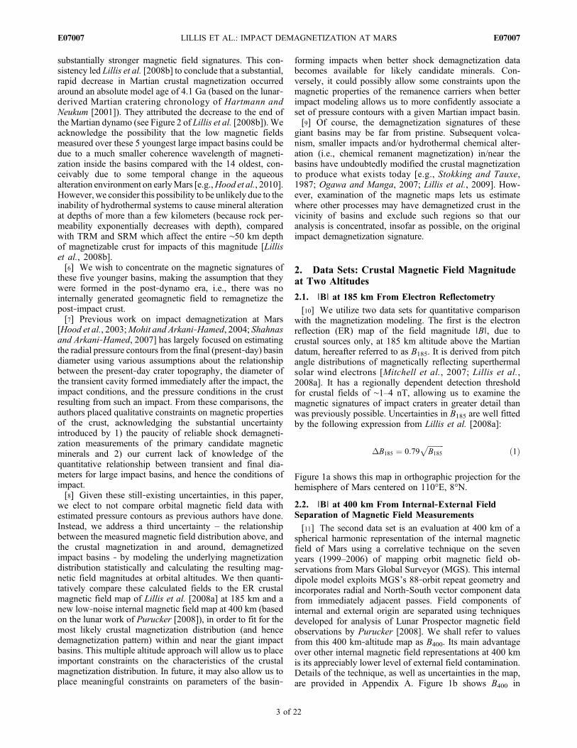
substantially stronger magnetic field signatures. This con-sistency led Lillis et al. [2008b] to conclude that a substantial,rapid decrease in Martian crustal magnetization occurredaround an absolute model age of 4.1 Ga (based on the lunar‐derived Martian cratering chronology of Hartmann andNeukum [2001]). They attributed the decrease to the end oftheMartian dynamo (see Figure 2 of Lillis et al. [2008b]). Weacknowledge the possibility that the low magnetic fieldsmeasured over these 5 youngest large impact basins could bedue to a much smaller coherence wavelength of magneti-zation inside the basins compared with the 14 oldest, con-ceivably due to some temporal change in the aqueousalteration environment on earlyMars [e.g.,Hood et al., 2010].However, we consider this possibility to be unlikely due to theinability of hydrothermal systems to cause mineral alterationat depths of more than a few kilometers (because rock per-meability exponentially decreases with depth), comparedwith TRM and SRM which affect the entire ∼50 km depthof magnetizable crust for impacts of this magnitude [Lilliset al., 2008b].[6] We wish to concentrate on the magnetic signatures of

these five younger basins, making the assumption that theywere formed in the post‐dynamo era, i.e., there was nointernally generated geomagnetic field to remagnetize thepost‐impact crust.[7] Previous work on impact demagnetization at Mars

[Hood et al., 2003;Mohit and Arkani‐Hamed, 2004; Shahnasand Arkani‐Hamed, 2007] has largely focused on estimatingthe radial pressure contours from the final (present‐day) basindiameter using various assumptions about the relationshipbetween the present‐day crater topography, the diameter ofthe transient cavity formed immediately after the impact, theimpact conditions, and the pressure conditions in the crustresulting from such an impact. From these comparisons, theauthors placed qualitative constraints on magnetic propertiesof the crust, acknowledging the substantial uncertaintyintroduced by 1) the paucity of reliable shock demagneti-zation measurements of the primary candidate magneticminerals and 2) our current lack of knowledge of thequantitative relationship between transient and final dia-meters for large impact basins, and hence the conditions ofimpact.[8] Given these still‐existing uncertainties, in this paper,

we elect to not compare orbital magnetic field data withestimated pressure contours as previous authors have done.Instead, we address a third uncertainty – the relationshipbetween the measured magnetic field distribution above, andthe crustal magnetization in and around, demagnetizedimpact basins ‐ by modeling the underlying magnetizationdistribution statistically and calculating the resulting mag-netic field magnitudes at orbital altitudes. We then quanti-tatively compare these calculated fields to the ER crustalmagnetic field map of Lillis et al. [2008a] at 185 km and anew low‐noise internal magnetic field map at 400 km (basedon the lunar work of Purucker [2008]), in order to fit for themost likely crustal magnetization distribution (and hencedemagnetization pattern) within and near the giant impactbasins. This multiple altitude approach will allow us to placeimportant constraints on the characteristics of the crustalmagnetization distribution. In future, it may also allow us toplace meaningful constraints on parameters of the basin‐

forming impacts when better shock demagnetization databecomes available for likely candidate minerals. Con-versely, it could possibly allow some constraints upon themagnetic properties of the remanence carriers when betterimpact modeling allows us to more confidently associate aset of pressure contours with a given Martian impact basin.[9] Of course, the demagnetization signatures of these

giant basins may be far from pristine. Subsequent volca-nism, smaller impacts and/or hydrothermal chemical alter-ation (i.e., chemical remanent magnetization) in/near thebasins have undoubtedly modified the crustal magnetizationto produce what exists today [e.g., Stokking and Tauxe,1987; Ogawa and Manga, 2007; Lillis et al., 2009]. How-ever, examination of the magnetic maps lets us estimatewhere other processes may have demagnetized crust in thevicinity of basins and exclude such regions so that ouranalysis is concentrated, insofar as possible, on the originalimpact demagnetization signature.

2. Data Sets: Crustal Magnetic Field Magnitudeat Two Altitudes

2.1. ∣B∣ at 185 km From Electron Reflectometry

[10] We utilize two data sets for quantitative comparisonwith the magnetization modeling. The first is the electronreflection (ER) map of the field magnitude ∣B∣, due tocrustal sources only, at 185 km altitude above the Martiandatum, hereafter referred to as B185. It is derived from pitchangle distributions of magnetically reflecting superthermalsolar wind electrons [Mitchell et al., 2007; Lillis et al.,2008a]. It has a regionally dependent detection thresholdfor crustal fields of ∼1–4 nT, allowing us to examine themagnetic signatures of impact craters in greater detail thanwas previously possible. Uncertainties in B185 are well fittedby the following expression from Lillis et al. [2008a]:

DB185 ¼ 0:79ffiffiffiffiffiffiffiffiffiB185

pð1Þ

Figure 1a shows this map in orthographic projection for thehemisphere of Mars centered on 110°E, 8°N.

2.2. ∣B∣ at 400 km From Internal‐External FieldSeparation of Magnetic Field Measurements

[11] The second data set is an evaluation at 400 km of aspherical harmonic representation of the internal magneticfield of Mars using a correlative technique on the sevenyears (1999–2006) of mapping orbit magnetic field ob-servations from Mars Global Surveyor (MGS). This internaldipole model exploits MGS’s 88‐orbit repeat geometry andincorporates radial and North‐South vector component datafrom immediately adjacent passes. Field components ofinternal and external origin are separated using techniquesdeveloped for analysis of Lunar Prospector magnetic fieldobservations by Purucker [2008]. We shall refer to valuesfrom this 400 km‐altitude map as B400. Its main advantageover other internal magnetic field representations at 400 kmis its appreciably lower level of external field contamination.Details of the technique, as well as uncertainties in the map,are provided in Appendix A. Figure 1b shows B400 in


3 of 22

orthographic projection for the hemisphere of Mars centeredon 110°E, 8°N.

3. Statistical Modeling of ImpactDemagnetization

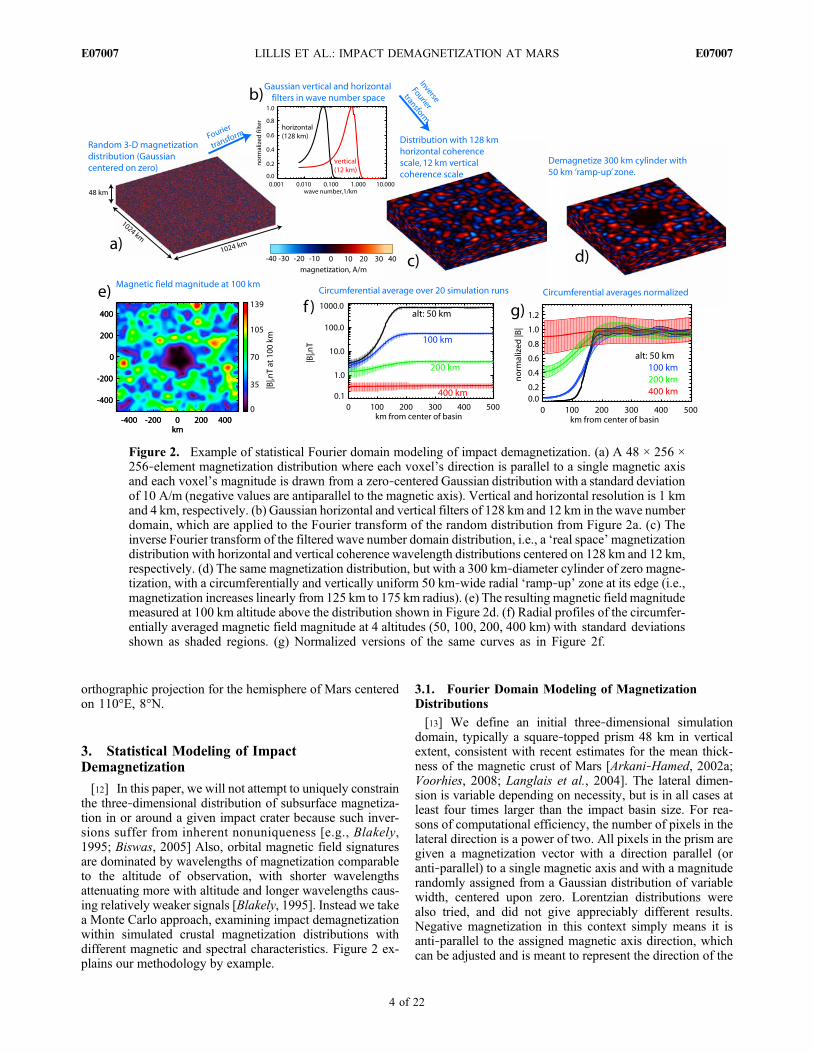
[12] In this paper, we will not attempt to uniquely constrainthe three‐dimensional distribution of subsurface magnetiza-tion in or around a given impact crater because such inver-sions suffer from inherent nonuniqueness [e.g., Blakely,1995; Biswas, 2005] Also, orbital magnetic field signaturesare dominated by wavelengths of magnetization comparableto the altitude of observation, with shorter wavelengthsattenuating more with altitude and longer wavelengths caus-ing relatively weaker signals [Blakely, 1995]. Instead we takea Monte Carlo approach, examining impact demagnetizationwithin simulated crustal magnetization distributions withdifferent magnetic and spectral characteristics. Figure 2 ex-plains our methodology by example.

3.1. Fourier Domain Modeling of MagnetizationDistributions

[13] We define an initial three‐dimensional simulationdomain, typically a square‐topped prism 48 km in verticalextent, consistent with recent estimates for the mean thick-ness of the magnetic crust of Mars [Arkani‐Hamed, 2002a;Voorhies, 2008; Langlais et al., 2004]. The lateral dimen-sion is variable depending on necessity, but is in all cases atleast four times larger than the impact basin size. For rea-sons of computational efficiency, the number of pixels in thelateral direction is a power of two. All pixels in the prism aregiven a magnetization vector with a direction parallel (oranti‐parallel) to a single magnetic axis and with a magnituderandomly assigned from a Gaussian distribution of variablewidth, centered upon zero. Lorentzian distributions werealso tried, and did not give appreciably different results.Negative magnetization in this context simply means it isanti‐parallel to the assigned magnetic axis direction, whichcan be adjusted and is meant to represent the direction of the

Figure 2. Example of statistical Fourier domain modeling of impact demagnetization. (a) A 48 × 256 ×256‐element magnetization distribution where each voxel’s direction is parallel to a single magnetic axisand each voxel’s magnitude is drawn from a zero‐centered Gaussian distribution with a standard deviationof 10 A/m (negative values are antiparallel to the magnetic axis). Vertical and horizontal resolution is 1 kmand 4 km, respectively. (b) Gaussian horizontal and vertical filters of 128 km and 12 km in the wave numberdomain, which are applied to the Fourier transform of the random distribution from Figure 2a. (c) Theinverse Fourier transform of the filtered wave number domain distribution, i.e., a ‘real space’magnetizationdistribution with horizontal and vertical coherence wavelength distributions centered on 128 km and 12 km,respectively. (d) The same magnetization distribution, but with a 300 km‐diameter cylinder of zero magne-tization, with a circumferentially and vertically uniform 50 km‐wide radial ‘ramp‐up’ zone at its edge (i.e.,magnetization increases linearly from 125 km to 175 km radius). (e) The resulting magnetic field magnitudemeasured at 100 km altitude above the distribution shown in Figure 2d. (f) Radial profiles of the circumfer-entially averaged magnetic field magnitude at 4 altitudes (50, 100, 200, 400 km) with standard deviationsshown as shaded regions. (g) Normalized versions of the same curves as in Figure 2f.


4 of 22

paleomagnetic field which, with geodynamo reversals, weassume originally magnetized the crust.[14] In the second step, we Fourier transform the mag-

netization magnitudes in the prism to frequency space, andthen apply a spatial filter. This filter can in theory be any-thing we wish: low‐pass, high pass, bandpass, notch, powerlaw etc., with all possible manner of roll‐off characteristics.It can also be anisotropic, i.e., different in each of the threedimensions. It is well beyond the scope of this paper tocover all these possible sorts of distributions and theireffects on orbital magnetic signatures; the parameter space issimply too vast. Instead we performed a limited examinationof some of these filters and determined that Gaussian filtersin wave number (i.e., spatial frequency) space resultedin demagnetization signatures that qualitatively match theobservations of extremely weak fields in the central regionsof basins (e.g., Figure 1) somewhat better than power lawdistributions which by definition include long wavelengthcomponents. It is worth noting that power law distributionshave reasonably well explained borehole and aeromagneticdata from terrestrial continental crust [e.g., Pilkington andTodoeschuck, 1993].[15] As shown in Figures 2a–2c, we apply these Gaussian

filters separately in the vertical and horizontal dimensions,with the filters purposely centered on specific values of ver-tical and horizontal wave numbers corresponding to spatialwavelengths or ‘coherence wavelengths’ (a term we shall userepeatedly). The width of these Gaussian filters was (some-what arbitrarily) chosen to be half of the central wave number.Narrower filters resulted in highly regular patterns that ap-peared physically unrealistic given our knowledge of ter-restrial magnetization distributions [e.g., Maus and Dimri,1995].[16] In the next step, we inverse Fourier transform the

filtered 3‐D frequency space distribution back to the originalspatial domain. In the example in Figure 2, the result is adistribution of magnetization with characteristic horizontaland vertical coherence wavelengths of 128 km and 12 km,respectively, i.e., these are the typical wavelengths overwhich the magnetization varies in the horizontal and verticaldirections. The typical coherence scale (i.e., size of a regionof coherent magnetization) is approximately half of thiswavelength, or 64 km in horizontal extent and 6 km invertical extent, as shown in Figure 2c. It is important toseparately model vertical and horizontal magnetic coherencescales because the processes that give rise to remanentmagnetization, such as the propagation of impact shockwaves, the pooling of subsurface water and the cooling ofimpact melt sheets and magmatic sills, are generallystrongly anisotropic because gravity only acts in the verticaldirection.[17] We then simulate impact demagnetization by reduc-

ing the magnetization in an azimuthally symmetric patternof arbitrary size, either uniformly or (if we wish) withadditional structure in the vertical direction. Discussions ofdetails of the simulated impact demagnetization are left tosection 5.

3.2. Calculating Magnetic Fields at Orbital Altitudes

[18] We calculate the resulting magnetic field at a givenaltitude (or set of altitudes) by summing the vector field dueto each flat horizontal layer of pixels using the method of

Blakely [1995]. This method assumes periodic boundaryconditions in the horizontal (but not vertical) directions sothat the field strength doesn’t fall off near the edge of thesimulation domain. The field magnitude at 100 km altitudeabove a 300 km‐diameter circular demagnetized zone isshown in Figure 2e.[19] Because the simulated magnetic field pattern comes

from a randomly produced magnetization distribution, wedo not try to fit these patterns to real magnetic fieldmaps (e.g.,Figure 1). Instead, we take the circumferential averagemagnetic field strength as a function of radius and averagethis over typically 20 random magnetization simulations, asshown in Figures 2f and 2g. These radial profiles of crustalmagnetic field can then be quantitatively fit to circumferen-tially averaged crustal magnetic field maps of Martian impactbasins at 185 km (ER) or 400 km (MAG), as discussed insection 2. Note that the particular magnetic intensity levels(in nT) shown in Figure 2f are not important for thisexample since magnetic field scales linearly with magneti-zation strength. Only the relative intensity, as a function ofradius, is important for this example.

3.3. Dependence of Magnetic Field Strengthon Magnetization Properties

[20] Even within the narrow context of our modelingframework, there are still 5 parameters that determine theaverage magnetic field magnitude ∣B∣ave measured above agiven magnetization distribution: 1) magnetization strength,2) magnetization direction, 3) vertical coherence wavelength,4) horizontal coherence wavelength and 5) altitude ofobservation. In addition, in trying to reproduce the observedradial magnetic profiles around large impact basins (e.g.,Figure 1), we will also attempt to constrain demagnetizationradius and demagnetization gradient width (i.e., ‘ramp‐up’distance as shown in Figure 2d). This is clearly too vast aparameter space to completely search for each basin. There-fore, we conducted a general examination of some of theseparameters to see if any simplifying assumptions can bemade before fitting to magnetic field observations. To dothis, we calculated ∣B∣ave as a function of various combina-tions of the aforementioned parameters. The results areshown in Figures 3, 4 and 5.We summarize the dependenciesbelow:3.3.1. Strength of Magnetization[21] At each given altitude, and for each coherence wave-

length, ∣B∣ave varies linearly with magnetization strength[Blakely, 1995].3.3.2. Total Thickness of Magnetized Layer[22] At our altitudes of interest and for layer thicknesses

less than or equal to 48 km [Voorhies, 2008], the magneticfield magnitude scales linearly with the thickness of themagnetized layer. Reasonable assumptions about heat flowand magnetic mineral carriers imply that the layer thicknessis unlikely to be much higher than this value [Arkani‐Hamed,2005].3.3.3. Direction of Magnetization[23] Just as the field of a magnetic dipole is symmetric

about the dipole axis, there is no dependence of ∣B∣ave on theazimuthal angle of magnetization. However, the asymmetryof a dipolar magnetic field (twice as strong at the pole versusthe equator) introduces a moderate dependence on the polarangle, though not a factor of two due to the canceling effects


5 of 22

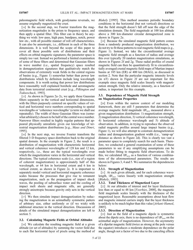
of adjacent regions of opposite magnetization. Horizontalmagnetization resulted in ∼30% weaker magnetic fieldscompared with vertical magnetization. This relationship islargely independent of horizontal coherence wavelength andaltitude as shown in Figure 3a. Figure 3b shows an exampleof the degree to which the magnetization polar angle affectsdemagnetization signatures. By assuming a polar angle of

45° in our fitting to observedmagnetic field profiles (section 5),we shall thus incur an error of not more than 20%.3.3.4. Vertical Coherence Wavelength[24] For our altitudes of concern above 185 km and for all

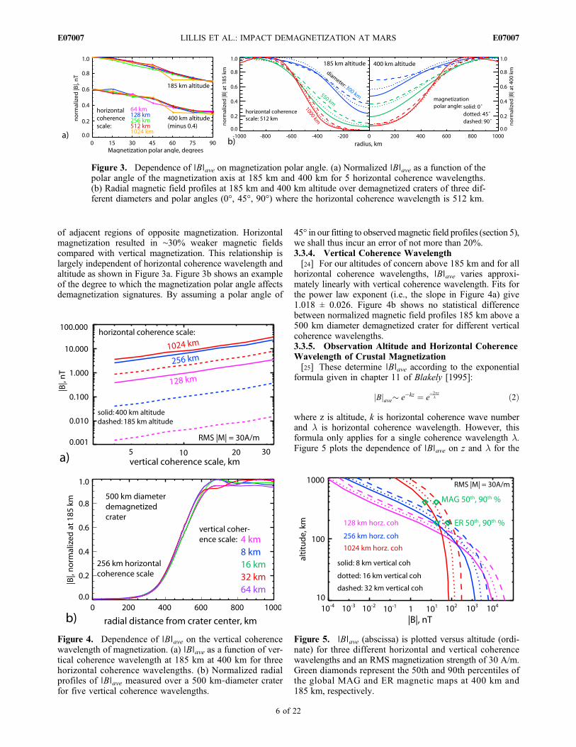
horizontal coherence wavelengths, ∣B∣ave varies approxi-mately linearly with vertical coherence wavelength. Fits forthe power law exponent (i.e., the slope in Figure 4a) give1.018 ± 0.026. Figure 4b shows no statistical differencebetween normalized magnetic field profiles 185 km above a500 km diameter demagnetized crater for different verticalcoherence wavelengths.3.3.5. Observation Altitude and Horizontal CoherenceWavelength of Crustal Magnetization[25] These determine ∣B∣ave according to the exponential

formula given in chapter 11 of Blakely [1995]:

Bj jave� e�kz ¼ e�2�z� ð2Þ

where z is altitude, k is horizontal coherence wave numberand l is horizontal coherence wavelength. However, thisformula only applies for a single coherence wavelength l.Figure 5 plots the dependence of ∣B∣ave on z and l for the

Figure 3. Dependence of ∣B∣ave on magnetization polar angle. (a) Normalized ∣B∣ave as a function of thepolar angle of the magnetization axis at 185 km and 400 km for 5 horizontal coherence wavelengths.(b) Radial magnetic field profiles at 185 km and 400 km altitude over demagnetized craters of three dif-ferent diameters and polar angles (0°, 45°, 90°) where the horizontal coherence wavelength is 512 km.

Figure 4. Dependence of ∣B∣ave on the vertical coherencewavelength of magnetization. (a) ∣B∣ave as a function of ver-tical coherence wavelength at 185 km at 400 km for threehorizontal coherence wavelengths. (b) Normalized radialprofiles of ∣B∣ave measured over a 500 km‐diameter craterfor five vertical coherence wavelengths.

Figure 5. ∣B∣ave (abscissa) is plotted versus altitude (ordi-nate) for three different horizontal and vertical coherencewavelengths and an RMS magnetization strength of 30 A/m.Green diamonds represent the 50th and 90th percentiles ofthe global MAG and ER magnetic maps at 400 km and185 km, respectively.


6 of 22

more realistic case of a Gaussian distribution of wave numbersaround a central wave number (as shown in Figure 2b) anda pre‐impact root mean square (RMS) magnetization strengthof 30 A/m. In this case, the dependence follows equation (2)up to altitudes slightly higher than l, above which the longerwavelengths from the edges of the Gaussian distributionbegin to dominate because they attenuate less quickly withaltitude. Interestingly, the 50th and 90th percentiles of theglobal MAG and ER maps are consistent with a globalaverage horizontal crustal magnetization coherence wave-length of ∼1000 km, indicating that the magnetized crust onMars is preserved coherently over truly enormous distancescompared with Earth. This finding is consistent with bestfit coherence wavelengths from comparing modeled toobserved magnetic profiles over impact basins and will bediscussed in section 6.[26] Therefore, when we attempt to model impact demag-

netization signatures for specific Martian basins there is noneed to run separate simulations for different values ofmagnetization polar angle, magnetization strength or verticalcoherence wavelength. We shall henceforth assume a verticalcoherence wavelength of 24 km, a pre‐impact RMS magne-tization strength of 10 A/m and a magnetization polar angleof 45°. These assumptions will simply mean a degeneracy(unavoidable in any case) between vertical coherence wave-length and magnetization strength, since ∣B∣ave has a lineardependence on both, in addition to the maximum error of20% due to magnetization direction.

3.4. Impact Demagnetization

[27] As mentioned in the introduction, when a large impactoccurs in the absence of a global dynamo magnetic field, weexpect substantial shock demagnetization. When consideringpost‐impact fractional demagnetization as a function ofradius and depth, there are two determining factors: 1) peakshock pressure contours and 2) the shock pressure versusmagnetization curve for the magnetic mineral(s) present(K. Louzada et al., Impact demagnetization of the Martiancrust: Current knowledge and future directions, submittedto Earth and Planetary Science Letters, 2010).[28] Although crater scaling can be used to estimate the

transient cavity diameter of simple (and to lesser extent,complex) craters and in turn the impact conditions (e.g.,impactor size and velocity) [e.g., Melosh, 1989], the forma-tion of large impact basins is still poorly understood. In par-ticular, the relationship between the transient basin andobservable final basin is unknown, making it difficult toapply crater scaling laws to large complex craters and ba-sins. Often, for the sake of convenience, the transient craterdiameter is taken to correspond to the inner ring scarp of animpact basin [e.g., Hood et al., 2003]. However, this is likelyan overestimate and the true transient cavity diameter liessomewhere between the complex crater scaled solution andthe inner ring scarp diameter. In the case of the Hellas basin,for example, the transient cavity diameter is likely betweenthe complex crater scaled solution of 800 km and theobserved flat‐floor diameter of 1300 to 1500 km [Louzadaand Stewart, 2009].[29] Figures 6a and 6b show the calculated peak shock

pressure contours for a 3‐dimensional CTH hydrocodesimulation [McGlaun et al., 1990] of a 250 km‐diameter

spherical impactor of density 3000 kg/m3, striking a layeredMars vertically at 9 km/s [Louzada and Stewart, 2009]. In thissimulation, a transient diameter of approximately 800 km isformed. In a region approximately the size of the impactorcentered below the impact point, the so‐called isobaric core,the peak shock pressure is typically constant [Pierazzo et al.,1997] and in this case well above ∼50 GPa. Outside of theisobaric core, the peak shock pressure decays both withdistance from the impact point and to zero at the surfacewhere there is a free‐surface boundary. Therefore, the radialpressure gradient is large so that pressure decays with dis-tance from the impact point along the surface much fasterthan with depth in the upper 50 km of the crust, where themagnetic minerals are likely to be located [e.g., Dunlop andArkani‐Hamed, 2005]. This is due to the curvature of theplanet and interference of shock waves at the crust‐mantleboundary layer [Louzada and Stewart, 2009]. At shallowdepth, the pressure decays rapidly to 1–2 GPa at ∼1000 kmradial distance. Outside this region, the decay is muchslower, with pressures >100 MPa out to >3000 km.[30] The density of Martian crust is reasonably well

constrained [Neumann et al., 2004, and references therein]as is the shock equation of state of basalt [Sekine et al.,2008], therefore, it is possible to calculate the pressurecontours for impacts into Martian materials using shockphysics codes as long as the impact parameters are known.However, for basin forming events, due to the uncertaintiesin the physics of late‐stage collapse and ring formation,transient craters identified in hydrocode simulations for agiven set of impact conditions cannot accurately predict thefinal size and character (multiringed or otherwise) of thebasin. Thus, the problem from our perspective lies in the factthat, for a given Martian impact basin such as Hellas orIsidis, of which only the final depth and diameter areknown, the peak pressure contours at the time of impactcannot be accurately determined at present.[31] Currently, limited experimental pressure demagneti-

zation data (static or shock) exists for magnetic minerals inthe appropriate pressure range (a few GPa). An example ofone such experiment is the static pressure demagnetizationof pyrrhotite by Rochette et al. [2003] which results incomplete demagnetization of pyrrhotite around 3 GPa(Figure 6c). However, pressure demagnetization curves foreach mineral are dependent on the magnetic domain size,coercivity of the magnetization, and chemistry of the indi-vidual minerals [e.g., Kletetschka et al., 2004; Bezaeva et al.,2010; Louzada et al., 2010; Gilder et al., 2006], making itdifficult to assign mineral specific demagnetization curves.[32] Furthermore, materials subjected to static and shock

experiments do not undergo the same loading paths andneither experiment type can reproduce the strain rates anddurations of pressure typical of a natural impact event. Inaddition, if kinetic processes (e.g., domain wall or dislocationmovement and fracturing) are important demagnetizationprocesses, then demagnetization results may be dependentupon experiment type (i.e., deformation mechanism). None-theless, numerous experiments on the main candidate mag-netic minerals on Mars (titanomagnetite, titanohematite, andpyrrhotite) indicate that low pressures of a few GPa result ina significant reduction of magnetization [e.g., Rochette et al.,2003]. Identifying mineral specific indicator pressures (e.g.,


7 of 22

complete demagnetization at a certain pressure level) remainsdifficult at present (Louzada et al., submitted manuscript,2010).[33] These current limitations lead us to avoid attempting

to calculate fractional demagnetization versus radius anddepth for individual impact basins and applying it to ourmagnetic modeling a priori for comparison to orbital mag-netic data. Instead, we choose a simpler approach and modelthe impact demagnetization with two parameters: thediameter of the demagnetized region and the distance overwhich the remaining fractional magnetization increases lin-early from 0% to 100% (or ‘ramp up’ distance), where the‘ramp‐up’ zone is symmetric about the demagnetizationradius, i.e., the fractional demagnetization is always 50% atthis radius (illustrated in Figure 14). In the example shown inFigure 2, the demagnetization diameter is 300 km and theramp‐up zone (which we call the ‘demagnetization gradientwidth’) is 50 km wide. Following the steep pressure contoursshown in Figure 6b, we assume no variation in magnetizationwith depth, i.e., cylindrically symmetric demagnetization.We recognize that this is an oversimplification of the impactdemagnetization process, but given the aforementioned un-certainties in peak pressure contours for a given basin, andas this is the first attempt to quantitatively model magnetic

field signatures with demagnetization patterns, we believe asimpler approach to be more illuminating.[34] It is hoped that, by placing constraints on these two

impact demagnetization parameters (demagnetization diam-eter and demagnetization gradient width), we may be able toplace joint constraints on peak pressure contours and shockpressure‐magnetization curves for the dominant minerals.However, before examining specific basins, it is instructive touse our impact demagnetization model to investigate thedegree to which the magnetic field signatures of even com-pletely demagnetized basins become less discernible withincreasing altitude. Readers interested only in the fittingresults may skip to section 5.

4. Detectability of Impact DemagnetizationSignatures at Orbital Altitudes

[35] Global magnetic field maps published by a number ofauthors [e.g., Cain et al., 2003; Langlais et al., 2004;Arkani‐Hamed, 2001, 2002b, 2004b], based in large parton the 400 km mapping orbit data set, fail to show cleardemagnetization signatures for any basins but Hellas, Utopia,Isidis and Argyre, all greater than 1100 km in diameter. TheER map at 185 km of Lillis et al. [2004, 2008a] additionally

Figure 6. (a and b) Peak pressure contours in 2 dimensions resulting from the CTH hydrocode simula-tion [McGlaun et al., 1990] of a 250 km‐diameter spherical impactor of density 3000 kg/m3, striking alayered Mars vertically at 9 km/s [Louzada and Stewart, 2009]. (c) The saturation remanence of pyrrhotiteas a function of static pressure from Rochette et al. [2003]. (d) Combination of the results in Figures 6band 6c to plot the fractional remaining magnetization as a function of depth and radius from the impactpoint. The upper 5 km of crust here is assumed not to be coherently magnetized due to impact gardeningand so can be ignored in Figure 6d. The abscissa axis in Figures 6b and 6d is distance from the impactpoint, along a great circle.


8 of 22

shows clear signatures over the 800 km–1200 km basinsPrometheus [Kletetschka et al., 2009], Ladon [Lillis et al.,2008a] and North Polar [Lillis et al., 2008b], plus severalcraters as small as ∼600 km, e.g., basins within AcidaliaPlanitia and the Margaritifer basin [Lillis et al., 2008a].[36] According to the catalog of Martian quasi‐circular

topographic depressions and circular thin‐crust areas of Frey[2006, 2008], there are more than 350 craters onMars between300 km and 600 km in diameter. Given the assumption thatthe Martian dynamo ceased at or somewhat before theUtopia impact ∼4.1 Ga [Lillis et al., 2008b], it is likely that asizable fraction of the craters in this size range formed in thepost‐dynamo era, and should therefore leave circular de-magnetized zones around the impact point. These zonesshould penetrate the entire thickness of the magnetic layer forbasins larger than 200 km, as can be deduced from analyticalradius‐pressure relationships [e.g., Melosh, 1989; Arkani‐Hamed, 2005], assuming that the same scaling relationshipshold for large basins as for smaller impact structures.[37] Therefore, why do we not observe hundreds or at

least many dozens of quasi‐circular ‘holes’ in the crustalmagnetic field pattern corresponding to the locations ofthese craters? This question has been addressed in recentpublications. Mohit and Arkani‐Hamed [2004] examinedmagnetization maps derived by magnetic inversion fromMGS MAG data by Arkani‐Hamed [2002a] for craters250 km to 500 km in diameter. However, the inherent non‐uniqueness of such inversions [Blakely, 1995] and the lim-ited spatial resolution of orbital magnetic field data suggestssubstantial uncertainty in the inferred magnetization dis-tributions shown in Figure 5 of Mohit and Arkani‐Hamed[2004] and hence the conclusion that substantial magneti-zation exists within many of the basins. Arkani‐Hamed[2005] commented that this inferred magnetization couldbe of very high coercivity in certain regions, preventing asubstantial fraction of magnetic crust from being demagne-tized by the impact. However, it is difficult to understandhow at least the transient cavity of an impact basin could notbe fully demagnetized, implying complete demagnetizationof the crust within the transient cavity radius for any rea-sonable thickness of magnetic crust (again assuming thesame scaling for large impact basins as for smaller impactstructures).[38] Similarly, Shahnas and Arkani‐Hamed [2007] argued

that the lack of weakening in magnetic field signatures overmost impact basins (excluding Isidis, Argyre and Hellas)leads to the statement that “there is no consistent evidencefor appreciable impact demagnetization of theMartian crust.”This conclusion is based partly on the assumption that ademagnetized zone comparable in size to the altitude ofobservation should be resolved in magnetic field maps, aseemingly reasonable assumption. However, to date, no rig-orous magnetization modeling has been applied to test thisassumption quantitatively, something we shall explore here.[39] One can imagine at least two reasons why we do not

observe hundreds of quasi‐circular ‘holes’ in the crustalmagnetic field pattern, including: 1) reduced size of thedemagnetized zone relative to the crater size (as suggestedby Shahnas and Arkani‐Hamed [2007]) and 2) the maskingof demagnetization signatures with increasing altitude. Theformer we cannot address without substantial advances inMartian giant impact simulation and shock demagnetization

experiments, as discussed in section 3.4. The latter, how-ever, can be investigated with our modeling frameworkexplained in section 3.1.[40] A quick observation of Figure 2 shows that, as the

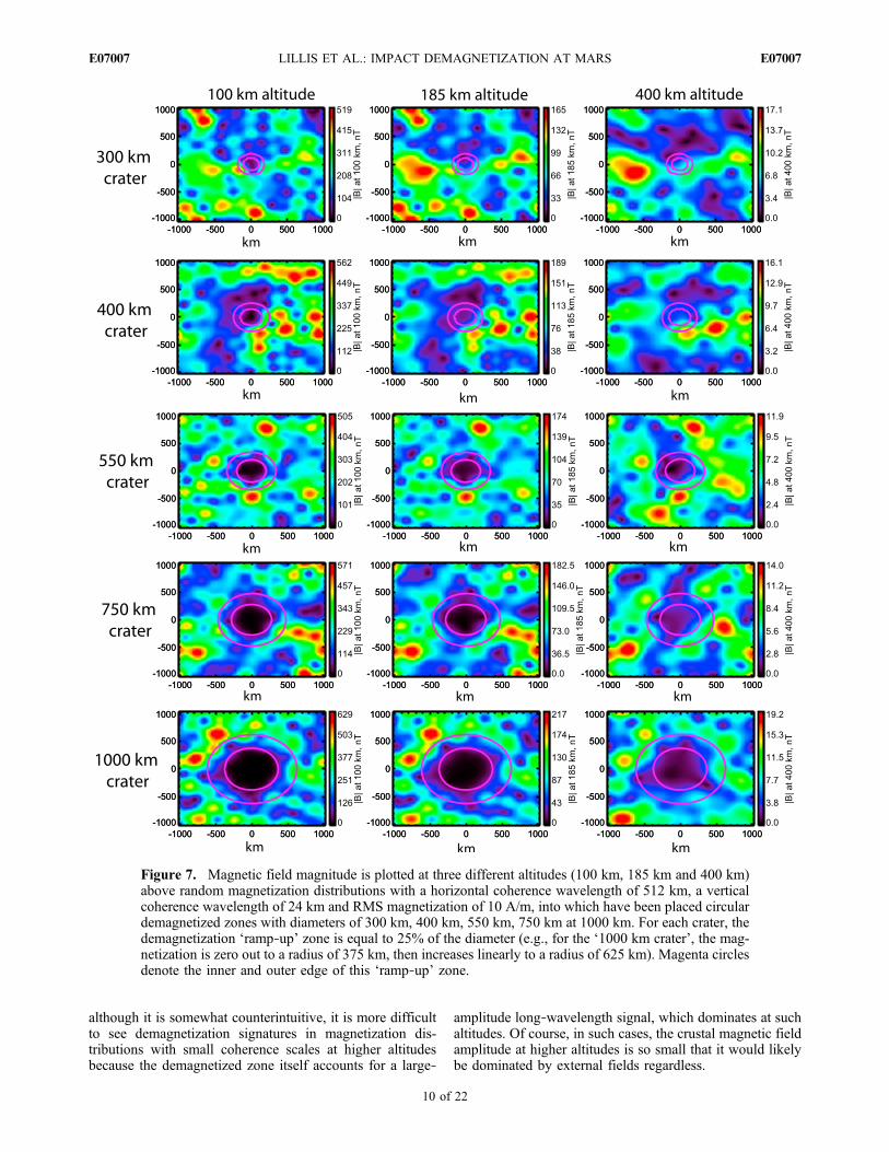
altitude of observation increases, the measured crustalmagnetic field strength rapidly decreases and that impactdemagnetization signatures become substantially less clear.A 300 km‐diameter demagnetized basin becomes essentiallyinvisible (particularly when standard deviations are takeninto account) in the magnetic field signature at 400 km.Figure 7 explores more of this parameter space, showing themagnetic field magnitude at 100 km, 185 km and 400 kmover demagnetized craters with diameters from 300 km to1000 km in a crust with a horizontal coherence wavelengthof 512 km (recall that Figure 5 showed that the dominantcoherence wavelength on Mars is certainly not smaller thanthis value). Figure 7 demonstrates that demagnetized areassmaller than ∼500 km cannot be recognized by eye at 185 km,while only demagnetized areas greater than ∼1000 kmdisplayrelatively unambiguous quasi‐circular features at 400 kmaltitude. Similar simulations were carried out using apower law distribution of modeled crustal magnetizationwith exponents between 1 and 4. In all cases, the large‐wavelength part of the spectrum resulted in substantialmagnetic field in the basin centers, i.e., less clear demag-netization signatures than those shown in Figure 7. Ofcourse, many more magnetic spectra could have been tried,e.g., power laws with cutoffs to omit the longest wave-lengths, with different roll‐off characteristics, but such anexhaustive parameter search is beyond the scope of thispaper.[41] Though instructive, plots like Figure 7 are subject to

the random fluctuations inherent in our technique and socannot be used to adequately determine these ‘limits ofdetection’ for demagnetized craters. For this purpose, weintroduce a useful quantity, the ratio (B<0.5R/B1.5–2R) ofmagnetic field magnitude inside 0.5 radii of the circulardemagnetized zone to the field magnitude between 1.5 and2 radii. The lower this ratio, the ‘clearer’ the demagnetiza-tion signature on a magnetic map. Figure 8 shows howB<0.5R/B1.5–2R changes for a range of crater sizes, coherencewavelengths and altitudes, calculated from circumferentialaverages over 20 pre‐impact random magnetization dis-tributions for each case. Not surprisingly, Figures 8a–8c showthat larger demagnetized craters have clearer magnetic sig-natures at all altitudes. Also, the ‘masking’ of the demag-netization signatures increases with altitude for all cratersizes for horizontal coherence wavelengths of 256 km and512 km, but for 1024 km the smaller craters (300, 400 km)are not easily visible at any altitude because they are com-parable in size to the natural undulations in the magnetiza-tion distribution. Figures 8d and 8e show a comprehensivepicture of the relationship between B<0.5R/B1.5–2R, coherencewavelength and demagnetized crater diameter at our twoaltitudes of observation.[42] It suggests that crater demagnetization signatures are

clearest for coherence wavelengths comparable to theobservation attitude (∼200 km in Figure 8d and 400–500 kmin Figure 8e). This is because the strongest magnetic fields arethose due to wavelengths of crustal magnetization (in thecrust surrounding the basin) that are comparable to theobservation attitude [Blakely, 1995, chapter 11]. In addition,


9 of 22

although it is somewhat counterintuitive, it is more difficultto see demagnetization signatures in magnetization dis-tributions with small coherence scales at higher altitudesbecause the demagnetized zone itself accounts for a large‐

amplitude long‐wavelength signal, which dominates at suchaltitudes. Of course, in such cases, the crustal magnetic fieldamplitude at higher altitudes is so small that it would likelybe dominated by external fields regardless.

Figure 7. Magnetic field magnitude is plotted at three different altitudes (100 km, 185 km and 400 km)above random magnetization distributions with a horizontal coherence wavelength of 512 km, a verticalcoherence wavelength of 24 km and RMS magnetization of 10 A/m, into which have been placed circulardemagnetized zones with diameters of 300 km, 400 km, 550 km, 750 km at 1000 km. For each crater, thedemagnetization ‘ramp‐up’ zone is equal to 25% of the diameter (e.g., for the ‘1000 km crater’, the mag-netization is zero out to a radius of 375 km, then increases linearly to a radius of 625 km). Magenta circlesdenote the inner and outer edge of this ‘ramp‐up’ zone.


10 of 22

[43] Figure 8 also demonstrates that, if the dominantcoherence wavelength on Mars is indeed on the order of∼1000 km as suggested by Figure 5 (and Figures 9–13presented later), then relatively clear demagnetization sig-natures should only be visible at 185 km and 400 km for

craters larger than ∼600 km and ∼1000 km, respectively.Thus it is possible to explain the lack of significant magneticfield weakening over moderate‐sized impact craters (300 km–600 km) at least partially in terms of masking of thedemagnetization signature with altitude, with the remainder

Figure 8. The variable B<0.5R/B1.5–2R (the ratio of magnetic field inside 0.5 basin radii to that between1.5 and 2 basin radii) is plotted as a function of altitude, coherence wavelength and demagnetizationdiameter. (a–c) Plotting of this ratio as a function of altitude for five crater diameters (300 km,400 km, 550 km, 750 km, 1000 km) and 3 coherence wavelengths (256 km, 512 km, 1024 km).(d and e) Plotting of the same ratio as a function of demagnetization diameter and horizontal coher-ence wavelength for our 2 observation altitudes: 185 km and 400 km.

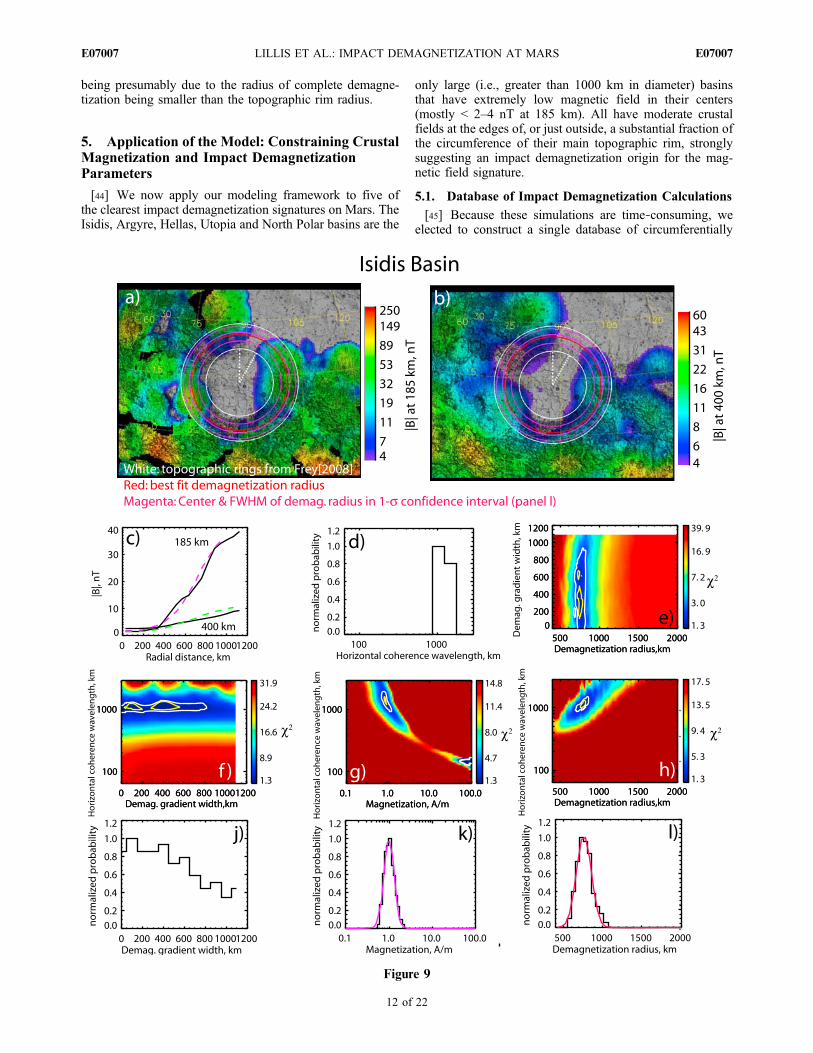
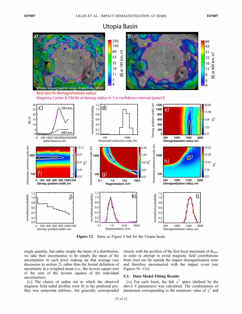
Figure 9. Demagnetization fitting results for the Isidis basin. (a and b) Magnetic field magnitude at 185 km and 400 km,respectively. Note the color scale is logarithmic and the colors are draped over shaded MOLA 1/16° topography [Smith et al.,2001]. The white rings represent the inner and outer topographic boundaries as defined by Frey [2006, 2008]. The red ringrepresents the demagnetization diameter of the c2 minimum. The 3 magenta rings represent the center and full width half maxvalues of the distribution of demagnetization diameter inside the 1‐sigma confidence interval (shown in Figure 9l). The whitedotted radial lines show the azimuth range over which radial profiles of B185 and B400 are averaged (values also given inTable 1). (c) Profiles of B185 and B400 shown as black lines, over which the best fit model predictions are plotted with pinkand green dashed lines, respectively. (d) A histogram of the distribution of values of horizontal coherence wavelength withinthe 1‐sigma confidence interval. (e–l) Plots arranged symmetrically, with demagnetization gradient width as the abscissa inthe left column, magnetization strength in the middle column and demagnetization radius in the right column and horizontalcoherence wavelength as the ordinate in the middle row. Figures 9e through 9h show four different two‐dimensional slicesof the 4‐dimensional c2 space defined by demagnetization radius, demagnetization gradient width, magnetization strengthand horizontal coherence wavelength. Each 2‐d slice correspondents to the c2 minimum in the other two dimensions. Thewhite contour corresponds to the 1‐sigma confidence interval (i.e., where c2 is less than 1.0+min (c2)). The yellow contourrepresents where c2 < 0.5 +min (c2). The latter contour is not always visible because nearest‐neighbor smoothing is appliedover each slice for display purposes. Figures 9j through 9l plot histograms of the distributions of demagnetization gradient,magnetization strength and demagnetization radius inside the 1‐sigma confidence interval. Gaussian curves (solid red/purplelines) are fit to the distributions of magnetization strength and demagnetization radius in Figures 9k and 9l, respectively, forthe purposes of determining center and FWHM values (given in Table 1).


11 of 22

being presumably due to the radius of complete demagne-tization being smaller than the topographic rim radius.

5. Application of the Model: Constraining CrustalMagnetization and Impact DemagnetizationParameters

[44] We now apply our modeling framework to five ofthe clearest impact demagnetization signatures on Mars. TheIsidis, Argyre, Hellas, Utopia and North Polar basins are the

only large (i.e., greater than 1000 km in diameter) basinsthat have extremely low magnetic field in their centers(mostly < 2–4 nT at 185 km). All have moderate crustalfields at the edges of, or just outside, a substantial fraction ofthe circumference of their main topographic rim, stronglysuggesting an impact demagnetization origin for the mag-netic field signature.

5.1. Database of Impact Demagnetization Calculations

[45] Because these simulations are time‐consuming, weelected to construct a single database of circumferentially

Figure 9


12 of 22

averaged radial magnetic field profiles (each one the averageof 20 separate simulations) at 185 km and 400 km altitude.As discussed earlier, each simulation had a magnetic layerstarting at 10 km depth, with thickness of 48 km, a magneti-zation polar angle of 45°, an RMS magnetization strength of10 A/m, and a vertical coherence wavelength of 24 km.[46] In order to build up adequate statistics, 20 simulations

were run for all combinations of the following ranges ofparameters, comprising a total of 187,200 simulations:

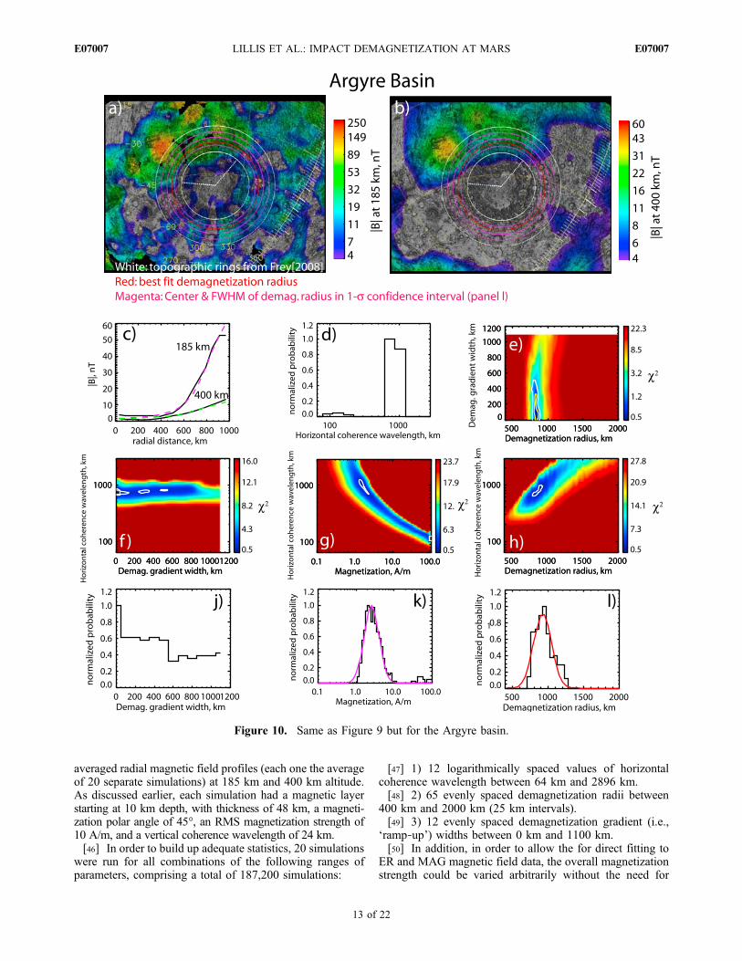
[47] 1) 12 logarithmically spaced values of horizontalcoherence wavelength between 64 km and 2896 km.[48] 2) 65 evenly spaced demagnetization radii between

400 km and 2000 km (25 km intervals).[49] 3) 12 evenly spaced demagnetization gradient (i.e.,

‘ramp‐up’) widths between 0 km and 1100 km.[50] In addition, in order to allow the for direct fitting to

ER and MAG magnetic field data, the overall magnetizationstrength could be varied arbitrarily without the need for

Figure 10. Same as Figure 9 but for the Argyre basin.


13 of 22

additional simulations (recall that magnetic field varies line-arly with magnetization for good values of other parameters).

5.2. Circumferential Averages of B185 and B400

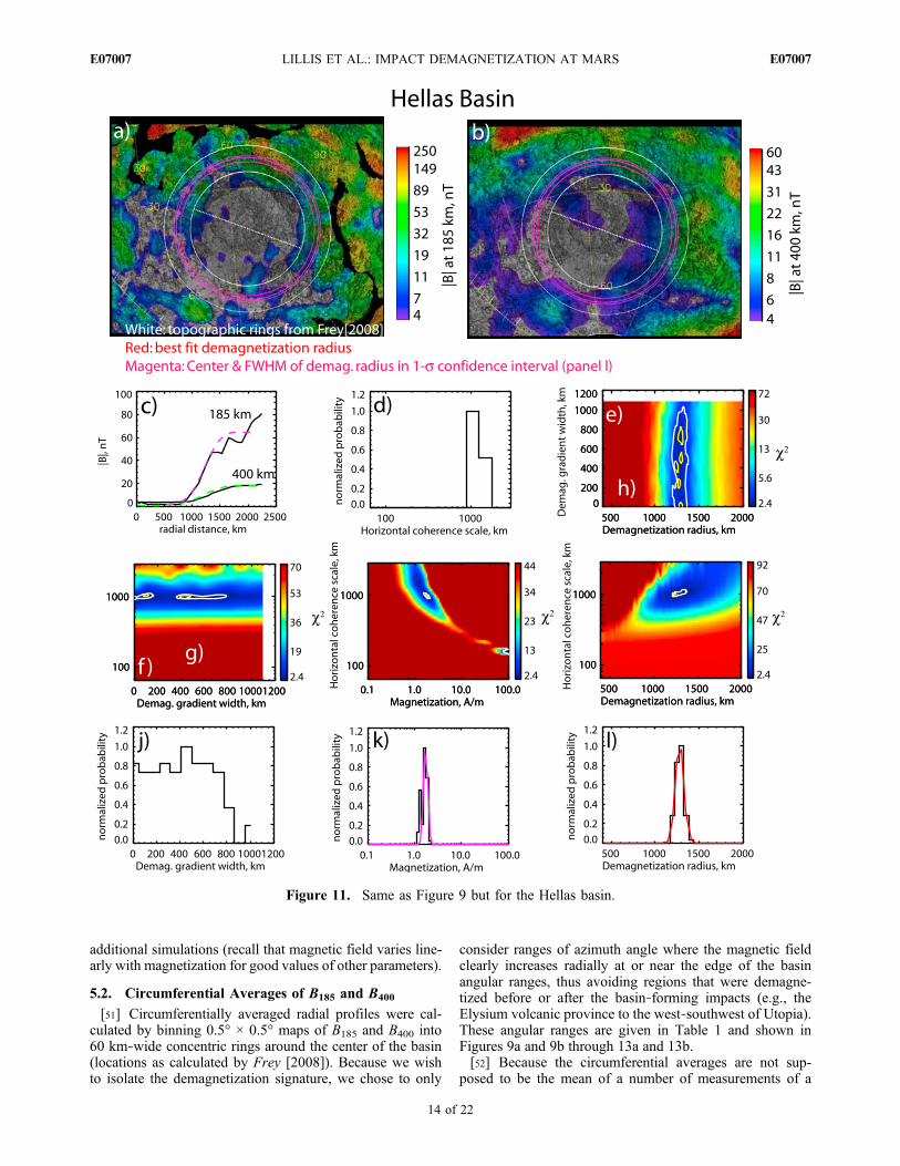
[51] Circumferentially averaged radial profiles were cal-culated by binning 0.5° × 0.5° maps of B185 and B400 into60 km‐wide concentric rings around the center of the basin(locations as calculated by Frey [2008]). Because we wishto isolate the demagnetization signature, we chose to only

consider ranges of azimuth angle where the magnetic fieldclearly increases radially at or near the edge of the basinangular ranges, thus avoiding regions that were demagne-tized before or after the basin‐forming impacts (e.g., theElysium volcanic province to the west‐southwest of Utopia).These angular ranges are given in Table 1 and shown inFigures 9a and 9b through 13a and 13b.[52] Because the circumferential averages are not sup-

posed to be the mean of a number of measurements of a

Figure 11. Same as Figure 9 but for the Hellas basin.


14 of 22

single quantity, but rather simply the mean of a distribution,we take their uncertainties to be simply the mean of theuncertainties in each pixel making up that average (seediscussion in section 2), rather than the formal definition ofuncertainty in a weighted mean (i.e., the inverse square rootof the sum of the inverse squares of the individualuncertainties).[53] The choice of radius out to which the observed

magnetic field radial profiles were fit to the predicted pro-files was somewhat arbitrary, but generally corresponded

closely with the position of the first local maximum of B185,in order to attempt to avoid magnetic field contributionsfrom crust too far outside the impact demagnetization zoneand therefore unconnected with the impact event (seeFigures 9c–13c).

5.3. Data‐Model Fitting Results

[54] For each basin, the full c2 space (defined by theabove 4 parameters) was calculated. The combinations ofparameters corresponding to the minimum value of c2 and

Figure 12. Same as Figure 9 but for the Utopia basin.


15 of 22

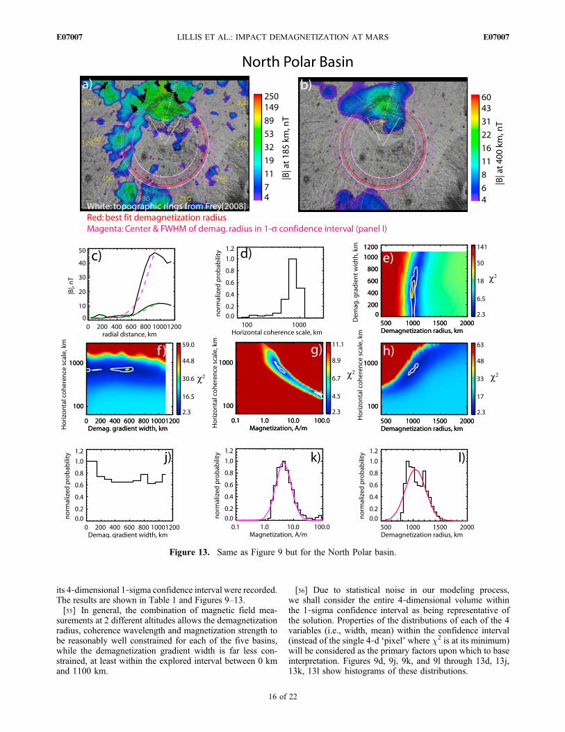
its 4‐dimensional 1‐sigma confidence interval were recorded.The results are shown in Table 1 and Figures 9–13.[55] In general, the combination of magnetic field mea-

surements at 2 different altitudes allows the demagnetizationradius, coherence wavelength and magnetization strength tobe reasonably well constrained for each of the five basins,while the demagnetization gradient width is far less con-strained, at least within the explored interval between 0 kmand 1100 km.

[56] Due to statistical noise in our modeling process,we shall consider the entire 4‐dimensional volume withinthe 1‐sigma confidence interval as being representative ofthe solution. Properties of the distributions of each of the 4variables (i.e., width, mean) within the confidence interval(instead of the single 4‐d ‘pixel’ where c2 is at its minimum)will be considered as the primary factors upon which to baseinterpretation. Figures 9d, 9j, 9k, and 9l through 13d, 13j,13k, 13l show histograms of these distributions.

Figure 13. Same as Figure 9 but for the North Polar basin.


16 of 22

5.4. Magnetization Coherence Wavelength

[57] Despite the somewhat coarse resolution of thecoherence wavelength parameter (given in section 5.1), the1‐sigma confidence intervals tell a consistent story regard-ing the dominant coherence wavelength in the regions sur-rounding these basins. The 1‐sigma interval mean value foreach of the basins is between ∼650 km and 1200 km asshown in Table 1 and Figures 9d–13d. The constraint oncoherence wavelength for North Polar basin is based on avery narrow azimuthal slice (∼60°) compared to the otherbasins (125°–330°, given in Table 1) and so does not havethe same statistical robustness, which should be kept inmind when considering the results.[58] Two important points need to be made regarding

these model results. The first point is that we have definedcoherence wavelength as being the full wavelength overwhich the magnetization varies within the model, whereas ifwe wish to think of the typical size of a single region ofcoherently magnetized crust, the half wavelength of magne-tization is more appropriate andwould therefore be ∼325 km–600 km. The second point is that these values are of courseonly valid within the context of our modeling framework,which makes the assumption of a single dominant coherencewavelength with some Gaussian distribution around it (seeFigure 2b). The structure of the real Martian crust is likely tobe richly complex with contributions at many coherencescales, though we cannot detect scales smaller than ∼100 kmwith any current data [Blakely, 1995]. These fitting resultswill be discussed further in the next (discussion) section.

5.5. Magnetization Strength

[59] The best fit values of the magnetization strengthshown in Table 1 are subject to the assumption of a mag-

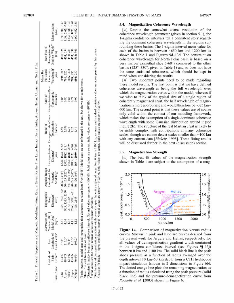
Figure 14. Comparison of magnetization‐versus‐radiuscurves. Shown in pink and blue are curves derived fromthe present work for Argyre and Hellas, respectively, forall values of demagnetization gradient width containedin the 1‐sigma confidence interval (see Figures 9j–13j)between 0 km and 1100 km. The solid black line is the peakshock pressure as a function of radius averaged over thedepth interval 10 km–60 km depth from a CTH hydrocodeimpact simulation (shown in 2 dimensions in Figure 6b).The dotted orange line plots the remaining magnetization asa function of radius calculated using the peak pressure (solidblack line) and the pressure‐demagnetization curve fromRochette et al. [2003] shown in Figure 6c.T

able

1.Phy

sicalPropertiesandMagnetic

Mod

eling/FittingResultsGiven

fortheFiveLarge

Impact

BasinsIsidis,Argyre,

Hellas,Utopia,

andNorth

Polar

Basin

Nam

e

Latitu

deof

Basin

Centera

East

Lon

gitude

ofBasin

Centera

Hartman

nan

dNeukum

[200

1]Mod

elAge

a

(Gyr)

Top

ograph

icRing

Diametersa

(km)

Ang

ular

Range

Con

sideredfor

Magnetic

Mod

elingb

Dem

agnetization

Diameter

c

(km)

Ratio

ofDem

agnetization/Inner

Top

ograph

icDiameter

Ratio

ofDem

agnetization/Outer

Top

ograph

icDiameter

MeanBest

FitLateral

Coh

erence

Wavelengthd

(km)

BestFits

ofDem

agnetization

GradientWidth

d,e

(km)

Magnetizationf

(A/m

)

Isidis

13.4°N

87.8°

3.81

1048

;13

52;18

4590

–60(330

°)12

98;15

73;17

641.50

0.85

1198

;21

745

5;32

50.71

;1.04

;1.37

Argyre

49.0°S

317.5°

4.04

905;

1315

;23

5050

–175

(125

°)15

72;18

82;21

112.07

80.80

761;

225

454;

354

1.58

;2.65

;4.39

Hellas

42.3°S

66.4°

4.07

2070

;30

8534

0–16

0(180

°)24

42;26

05;26

791.26

0.84

1152

;20

244

1;28

31.59

;1.66

;1.93

Utopia

45.0°N

115.5°

4.11

2360

;33

80;42

1080

–285

(205

°)28

45;31

21;34

101.32

0.74

788;

295

453;

336

0.46

;0.73

;1.30

N.Polar

80.0°N

195.2°

4.12

1486

;21

4560

–120

(60°)

1681

;20

89;24

661.41

0.97

650;

239

518;

361

2.09

;4.52

;8.88

a Basin

locatio

ns,mod

elages

andtopo

graphicring

diam

etersaretakenfrom

Frey[200

8].Mod

elages

areno

treferenced

inthetext,bu

tshow

nforcompleteness.

bHere0°

iseastfrom

center

ofbasin.

c Gaussianfitinside

1‐sigm

aconfidence

interval.Normal

values

arecenter

−HWHM,bo

ldvalues

arecenter,italic

values

arecenter

+HWHM.

dBoldvalues

arethemean;

norm

alvalues

arestandard

deviation.

e Distributions

ofdemagnetizationgradient

width

generally

span

theentireexplored

rang

efrom

0km

to11

00km

,so

meanandstandard

deviationvalues

areaccompanied

bythiscaveat.

f Gaussianfitinside

1‐sigm

aconfidence

interval.Normal

values

arecenter

−HWHM,bo

ldvalues

arecenter,italic

values

arecenter

+HWHM.


17 of 22

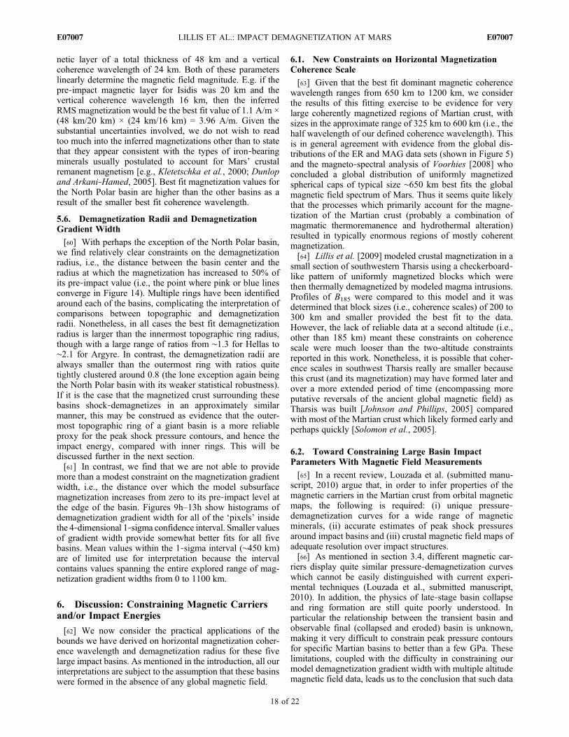
netic layer of a total thickness of 48 km and a verticalcoherence wavelength of 24 km. Both of these parameterslinearly determine the magnetic field magnitude. E.g. if thepre‐impact magnetic layer for Isidis was 20 km and thevertical coherence wavelength 16 km, then the inferredRMS magnetization would be the best fit value of 1.1 A/m ×(48 km/20 km) × (24 km/16 km) = 3.96 A/m. Given thesubstantial uncertainties involved, we do not wish to readtoo much into the inferred magnetizations other than to statethat they appear consistent with the types of iron‐bearingminerals usually postulated to account for Mars’ crustalremanent magnetism [e.g., Kletetschka et al., 2000; Dunlopand Arkani‐Hamed, 2005]. Best fit magnetization values forthe North Polar basin are higher than the other basins as aresult of the smaller best fit coherence wavelength.

5.6. Demagnetization Radii and DemagnetizationGradient Width

[60] With perhaps the exception of the North Polar basin,we find relatively clear constraints on the demagnetizationradius, i.e., the distance between the basin center and theradius at which the magnetization has increased to 50% ofits pre‐impact value (i.e., the point where pink or blue linesconverge in Figure 14). Multiple rings have been identifiedaround each of the basins, complicating the interpretation ofcomparisons between topographic and demagnetizationradii. Nonetheless, in all cases the best fit demagnetizationradius is larger than the innermost topographic ring radius,though with a large range of ratios from ∼1.3 for Hellas to∼2.1 for Argyre. In contrast, the demagnetization radii arealways smaller than the outermost ring with ratios quitetightly clustered around 0.8 (the lone exception again beingthe North Polar basin with its weaker statistical robustness).If it is the case that the magnetized crust surrounding thesebasins shock‐demagnetizes in an approximately similarmanner, this may be construed as evidence that the outer-most topographic ring of a giant basin is a more reliableproxy for the peak shock pressure contours, and hence theimpact energy, compared with inner rings. This will bediscussed further in the next section.[61] In contrast, we find that we are not able to provide

more than a modest constraint on the magnetization gradientwidth, i.e., the distance over which the model subsurfacemagnetization increases from zero to its pre‐impact level atthe edge of the basin. Figures 9h–13h show histograms ofdemagnetization gradient width for all of the ‘pixels’ insidethe 4‐dimensional 1‐sigma confidence interval. Smaller valuesof gradient width provide somewhat better fits for all fivebasins. Mean values within the 1‐sigma interval (∼450 km)are of limited use for interpretation because the intervalcontains values spanning the entire explored range of mag-netization gradient widths from 0 to 1100 km.

6. Discussion: Constraining Magnetic Carriersand/or Impact Energies

[62] We now consider the practical applications of thebounds we have derived on horizontal magnetization coher-ence wavelength and demagnetization radius for these fivelarge impact basins. As mentioned in the introduction, all ourinterpretations are subject to the assumption that these basinswere formed in the absence of any global magnetic field.

6.1. New Constraints on Horizontal MagnetizationCoherence Scale

[63] Given that the best fit dominant magnetic coherencewavelength ranges from 650 km to 1200 km, we considerthe results of this fitting exercise to be evidence for verylarge coherently magnetized regions of Martian crust, withsizes in the approximate range of 325 km to 600 km (i.e., thehalf wavelength of our defined coherence wavelength). Thisis in general agreement with evidence from the global dis-tributions of the ER and MAG data sets (shown in Figure 5)and the magneto‐spectral analysis of Voorhies [2008] whoconcluded a global distribution of uniformly magnetizedspherical caps of typical size ∼650 km best fits the globalmagnetic field spectrum of Mars. Thus it seems quite likelythat the processes which primarily account for the magne-tization of the Martian crust (probably a combination ofmagmatic thermoremanence and hydrothermal alteration)resulted in typically enormous regions of mostly coherentmagnetization.[64] Lillis et al. [2009] modeled crustal magnetization in a

small section of southwestern Tharsis using a checkerboard‐like pattern of uniformly magnetized blocks which werethen thermally demagnetized by modeled magma intrusions.Profiles of B185 were compared to this model and it wasdetermined that block sizes (i.e., coherence scales) of 200 to300 km and smaller provided the best fit to the data.However, the lack of reliable data at a second altitude (i.e.,other than 185 km) meant these constraints on coherencescale were much looser than the two‐altitude constraintsreported in this work. Nonetheless, it is possible that coher-ence scales in southwest Tharsis really are smaller becausethis crust (and its magnetization) may have formed later andover a more extended period of time (encompassing moreputative reversals of the ancient global magnetic field) asTharsis was built [Johnson and Phillips, 2005] comparedwith most of the Martian crust which likely formed early andperhaps quickly [Solomon et al., 2005].

6.2. Toward Constraining Large Basin ImpactParameters With Magnetic Field Measurements

[65] In a recent review, Louzada et al. (submitted manu-script, 2010) argue that, in order to infer properties of themagnetic carriers in the Martian crust from orbital magneticmaps, the following is required: (i) unique pressure‐demagnetization curves for a wide range of magneticminerals, (ii) accurate estimates of peak shock pressuresaround impact basins and (iii) crustal magnetic field maps ofadequate resolution over impact structures.[66] As mentioned in section 3.4, different magnetic car-

riers display quite similar pressure‐demagnetization curveswhich cannot be easily distinguished with current experi-mental techniques (Louzada et al., submitted manuscript,2010). In addition, the physics of late‐stage basin collapseand ring formation are still quite poorly understood. Inparticular the relationship between the transient basin andobservable final (collapsed and eroded) basin is unknown,making it very difficult to constrain peak pressure contoursfor specific Martian basins to better than a few GPa. Theselimitations, coupled with the difficulty in constraining ourmodel demagnetization gradient width with multiple altitudemagnetic field data, leads us to the conclusion that such data


18 of 22

are very unlikely to yield meaningful constraints on thespecific carriers ofMartian crustal remanent magnetism, evenin the event of more accurate simulations of peak pressurecontours.[67] However, we have demonstrated in this paper that the

average radius of demagnetization can be constrained (in thecase of Hellas, quite narrowly) even in the absence of aneffective constraint on the demagnetization gradient width.Figure 14 compares ranges of demagnetization‐radius curvesthat match the orbital magnetic field data (i.e., fall withinthe 1‐sigma confidence interval) for the Argyre and Hellasbasins, with a depth‐averaged demagnetization‐radiuscurve calculated fromCTH‐simulated peak pressure contoursand using the static pressure‐demagnetization curve forpyrrhotite from Rochette et al. [2003].[68] This implies that, if we instead exploit the fact

that many magnetic minerals have very similar pressure‐demagnetization curves, we can use the results of manyimpact simulations to predict a family of demagnetization‐versus‐radius curves (like the orange dotted line in Figure 15),each one corresponding to set of impact conditions. Withinthe modeling framework presented in this paper, eachmember of the curve family will correspond to an orbitalmagnetic signature, which can then be compared to cir-cumferentially averaged radial magnetic field profiles likethose shown in Figures 9c–13c. This should in theory allowus to constrain impact energies and peak pressure contoursfor specific Martian basins and should therefore enable us tobetter understand the complex processes involved in theformation of large basins (i.e., multiple rings scarps etc.).This aspect will be the focus of future work.[69] The fact that the ratio between the outer topographic

ring radius identified by Frey [2008] and the best meandemagnetization radius is very close to 0.8 for the 4 clearestlarge basins (Isidis, Argyre, Utopia and Hellas, see Table 1)suggests that similar basin‐forming mechanics and shockdemagnetization processes occurred for all four impacts andalso that the outer topographic ring diameter may be a betterproxy compared with inner rings for peak impact pressures.Future hydrocode simulation work should further elucidatethese processes.

7. Conclusions

[70] In this paper we have presented a framework formodeling statistically the circumferentially averaged mag-netic field signature, at orbital altitudes, of shock‐demagnetized impact basins on Mars. We have investigated7 of the factors which affect these signatures: the magneti-zation strength, primary direction, thickness and vertical andhorizontal coherence wavelengths, as well as the demagne-tization radius and the width of the demagnetization gradient(or ‘ramp‐up’) zone caused by impact shock. We have alsoused magnetic field magnitude data at 2 different altitudesover 5 large apparently demagnetized (and therefore probablypost‐dynamo) impact structures, along with this modelingframework, in order to place constraints on the aforemen-tioned factors.[71] Our primary conclusions are:[72] 1) The dominant lateral coherence wavelength of

Martian crustal magnetization in the vicinity of these 5 largeimpact basins (and likely globally), as we have defined it, is

in the range of ∼650 km to 1200 km. This corresponds totypically enormous regions of coherently magnetized crustin the size range of ∼325 km to 600 km. Table 1 and Figures 6and 9–13 display this effect.[73] 2) The magnetic field observed over a circular

demagnetized region depends in a complex and somewhatnonintuitive manner on the relationship between the size ofthe region, the coherence wavelength of the pre‐impactmagnetization and the altitude of observation. A primeconsequence of this is that increasing altitude masks thedemagnetization signature such that somewhat clear demag-netization signatures should only be visible in magnetic fieldmaps at 185 km and 400 km altitude for demagnetizationdiameters larger than ∼600 km and ∼1000 km, respectively.Thus it is possible to explain the lack of significant mag-netic field weakening over moderate‐sized impact craters(300 km–600 km) at least partially in terms of this maskingwith the remainder possibly due to the radius of completedemagnetization being smaller than the topographic rimradius. Therefore, lower altitude data orbital data, such as weare expecting from the 2013 MAVEN mission (periapsisaltitude: 120 km–150 km), will make available substantiallymore craters for magnetic analysis.[74] 3) Using this kind of statistical modeling, along with

multiple altitude magnetic field data, averaged demagneti-zation diameters can be constrained for these basins, even inthe absence of constraints on the associated demagnetizationgradient widths. The ratio of these demagnetization dia-meters to the outer topographic ring diameter is close to0.8 for Isidis, Hellas, Argyre and Utopia, suggesting thatsimilar basin‐forming and shock demagnetization pro-cesses occurred in each of these four ancient impacts.[75] 4) Even if orbital magnetic field data cannot ever

meaningfully constrain magnetic mineralogy on Mars, thesimilarity of pressure‐demagnetization curves for manymagnetic minerals suggests that such data may lead, if usedin conjunction with impact simulations, to improved con-straints on peak shock pressure contours and impact ener-gies for specific Martian impact basins. This will improveour understanding of the formation of such basins.

Appendix A: Derivation of a New InternalMagnetic Field Model of Mars Based on MappingOrbit Observations Using a Correlative Approach

[76] The technique of developing a lower‐noise globalmap of the internal magnetic field of a planet, described indetail by Purucker [2008] for Lunar Prospector observationsof the lunar magnetic field, has been adapted for Mars in thiswork. It uses a correlative technique on the seven years(1999–2006) of mapping orbit magnetic field observationsfrom Mars Global Surveyor (MGS). The technique is aspace domain approach using three adjacent passes separatedin space by less than 1 degree of longitude, hence the derivedmagnetic field parameters are most sensitive to commoninternal crustal sources. An equivalent source formulation inspherical coordinates [Dyment and Arkani‐Hamed, 1998] isused, with the magnetized Martian crust divided into blocks,each of which is assumed to have a magnetic dipole at itscenter. Using the observations of the vertical and north‐south magnetic field, the magnitude of a series of horizontaldipoles located under the middle pass are calculated using a


19 of 22

conjugate gradient, iterative approach [Purucker et al.,1996]. This provides an analytic means of continuing thedata to a constant surface of 400 km above the mean Martianradius. The orbit characteristics of Lunar Prospector andMGS differ, and the basic repeat cycle of MGS is 88‐orbits,in which the orbits repeat approximately weekly.[77] The MGS maps were made only from night side data,

acquired at 0200 local time. The altitude‐normalized mag-netic field from the night side is used to build a model inwhich 99% of the 180 by 180 bins covering the Martiansurface are filled. The only unfilled bins are associated withthe polar gap, which extends from 87 degrees to the pole,and a few unpopulated bins between 85 and 87 degreesNorth latitude. The global model is then used to construct adegree 90 spherical harmonic model of the field via theDriscoll & Healy sampling theorem [Driscoll and Healy,1994]. Terms up to about degree 51 are robust, as shownby the increase in power beginning at that degree, and soonly those terms are used in evaluating the crustal magnetic

Figure A1. Comparison of 400 km altitude evaluations of the internal dipole model of Langlais, Puruckerand Mandea (LPM) [Langlais et al., 2004] and the correlative model used in the present work. The colorscale is highly nonuniform and emphasizes differences between small values of magnetic field magnitude.The contribution from non‐crustal sources varies geographically and ranges from 3 nT to 5 nT in the LPMmodel and from 1.0 nT to 2.5 nT in the correlative model.

Figure A2. The average error DB400 (equation (A1)) isplotted as a function of B400 for 3 different values of Bext,with the assumption that DBcal = 0.5 nT.


20 of 22

field magnitude map we use in the present work, which is ata constant altitude of 400 km, hereafter referred to as B400.Figure A1 demonstrates that the map of used in this workhas approximately 50% lower non‐crustal noise than theequivalent dipole magnetic model of Langlais et al. [2004].[78] The spherical harmonic solution, and a 2 degree

grid evaluated using spherical harmonic degrees 1–51,can be found at http://core2.gsfc.nasa.gov/research/purucker/mars2009. The technique is described in detail in Purucker[2008].[79] We derive the uncertainty in B400 first by expres-

sing the magnitude of the crustal‐only magnetic field, Bc,in terms of the magnitudes of the external (i.e., non‐crustal)field Bext and the total magnetic field, B400 (i.e., the vector sumof Bc and Bext):

Bc ¼ �Bext cos � þffiffiffiffiffiffiffiffiffiffiffiffiffiffiffiffiffiffiffiffiffiffiffiffiffiffiffiffiffiffiffiffiffiB2400 � B2

ext sin2 �

q;

where h is the angle between the vectorsBext andBc. The firstcomponent of the error in B400 is thus the difference inmagnitudes between Bc and B400, averaged over all values ofh. The second component is simply the calibration error of theMGS magnetometer, DBcal (∼0.5 nT) [Acuña et al., 2001].These two components are added in quadrature to give thetotal error DB400:

DB400 ¼"DB2

cal þ B400 þ 1

2�

Z2�0

�Bext cos �

�ffiffiffiffiffiffiffiffiffiffiffiffiffiffiffiffiffiffiffiffiffiffiffiffiffiffiffiffiffiffiffiffiffiB2400 � B2

ext sin2 �

q �d�

!2#1

2

ðA1Þ

We estimate themagnitude of the external fields present in theglobalmap ofDB400 to be 1.5–2.5 nT based onmeasurementsin regions, such as parts of Tharsis, where crustal fields at185 km are known to be <1 nT [Lillis et al., 2009]. Figure A2plotsDB400 as a function of B400 for three different values ofBext. The functional form in equation (A1) is used in the fittingprocedure described in section 5.

[80] Acknowledgments. We wish to thank an anonymous reviewerfor some helpful suggestions. This work was supported by the NASA MarsData Analysis program (grant NNX07AN94G) and Mars FundamentalResearch program (grants NNX09AN18G and NNX07AQ69G).

ReferencesAcuña, M. H., et al. (1999), Global distribution of crustal magnetizationdiscovered by the Mars Global Surveyor MAG/ER experiment, Science,284, 790–793, doi:10.1126/science.284.5415.790.

Acuña, M. H., et al. (2001), Magnetic field of Mars: Summary of resultsfrom the aerobraking and mapping orbits, J. Geophys. Res., 106,23,403–23,417.

Arkani‐Hamed, J. (2001), A 50‐degree spherical harmonic model of themagnetic field of Mars, J. Geophys. Res., 106, 23,197–23,208,doi:10.1029/2000JE001365.

Arkani‐Hamed, J. (2002a), Magnetization of the Martian crust, J. Geophys.Res., 107(E5), 5032, doi:10.1029/2001JE001496.

Arkani‐Hamed, J. (2002b), An improved 50‐degree spherical harmonicmodel of the magnetic field of Mars derived from both high‐altitude andlow‐altitude datasets, J. Geophys. Res., 107(E10), 5083, doi:10.1029/2001JE001835.

Arkani‐Hamed, J. (2004a), Timing of the Martian core dynamo, J. Geophys.Res., 109, E03006, doi:10.1029/2003JE002195.

Arkani‐Hamed, J. (2004b), A coherent model of the crustal field of Mars,J. Geophys. Res., 109, E09005, doi:10.1029/2004JE002265.

Arkani‐Hamed, J. (2005), Magnetic crust of Mars, J. Geophys. Res., 110,E08005, doi:10.1029/2004JE002397.

Bezaeva, N. S., J. Gattacceca, P. Rochette, R. A. Sadykov, and V. I. Trukhin(2010), An overview of the demagnetization of terrestrial and extraterres-trial rocks under hydrostatic pressure up to 1.2 GPa, Phys. Earth Planet.Inter., 179, 7–20, doi:10.1016/j.pepi.2010.01.004.

Biswas, R. (2005), Nonuniqueness of the modeled magnetization factorsused in determining paleopoles on Mars, Masters thesis, Southern Ill.Univ. at Carbondale, Carbondale.

Blakely, R. J. (1995), Potential Theory in Gravity and Magnetic Applica-tions, Cambridge Univ. Press, Cambridge, U. K., doi:10.1017/CBO9780511549816.

Cain, J. C., B. B. Ferguson, and D. Mozoni (2003), An n = 90 internalpotential function of the Martian crustal magnetic field, J. Geophys.Res., 107, 108(E2), 5008, doi:10.1029/2000JE001487.

Carporzen, L., S. A. Gilder, and R. J. Hart (2005), Palaeomagnetism of theVredefort meteorite crater and implications for craters on Mars, Nature,435, 198–201, doi:10.1038/nature03560.

Cisowski, S. M., and M. Fuller (1978), The effect of shock on the magne-tism of terrestrial rocks, J. Geophys. Res., 83, 3441–3458, doi:10.1029/JB083iB07p03441.

Driscoll, J. R., and D. M. Healy (1994), Computing Fourier transforms andconvolutions on the 2‐sphere, Adv. Appl. Math., 15(2), 202–250,doi:10.1006/aama.1994.1008.

Dunlop, D. J., and J. Arkani Hamed (2005),Magnetic minerals in theMartiancrust, J. Geophys. Res., 110, E12S04, doi:10.1029/2005JE002404.

Dyment, J., and J. Arkani‐Hamed (1998), Equivalent source magneticdipoles revisited, Geophys. Res. Lett., 25, 2003–2006, doi:10.1029/98GL51331.

Frey, H. V. (2006), Impact constraints on, and a chronology for, majorevents in early Mars history, J. Geophys. Res., 111, E08S91,doi:10.1029/2005JE002449.

Frey, H. (2008), Ages of very large impact basins on Mars: Implications forthe late heavy bombardment in the inner solar system, Geophys. Res.Lett., 35, L13203, doi:10.1029/2008GL033515.

Garrick‐Bethell, I., B. P. Weiss, D. L. Shuster, and J. Buz (2009), Earlylunar magnetism, Science, 323, 356–359, doi:10.1126/science.1166804.

Gattacceca, J., L. Berthe, M. Boustie, F. Vadeboin, P. Rochette, and T. deResseguier (2008), On the efficiency of shock magnetization processes,Phys. Earth Planet. Inter., 166, 1–10.

Gilder, S. A., M. Le Goff, and J. C. Chervin (2006), Static stress demagne-tization of single and multi‐domain magnetite with implications for mete-orite impacts, High Pressure Res., 26(4), 539–547, doi:10.1080/08957950601092085.

Grant, F. S. (1985), Aeromagnetics, geology and ore environments: 1. Mag-netite in igneous, sedimentary and metamorphic rocks: An overview,Geoexploration, 23, 303–333, doi:10.1016/0016-7142(85)90001-8.

Hartmann, W. K., and G. Neukum (2001), Cratering chronology and theevolution of Mars, Space Sci. Rev., 96, 165–194, doi:10.1023/A:1011945222010.

Hood, L. L., N. C. Richmond, E. Pierazzo, and P. Rochette (2003), Distri-bution of crustal magnetic fields on Mars: Shock effects of basin‐formingimpacts, Geophys. Res. Lett., 30(6), 1281, doi:10.1029/2002GL016657.

Hood, L. L., K. P. Harrison, B. Langlais, R. J. Lillis, F. Poulet, and D. A.Williams (2010) Magnetic anomalies near Apollinaris Patera and theMedusae Fossae Formation in Lucus Planum,Mars, Icarus, 208, 118–131.

Johnson, C. L., and R. J. Phillips (2005), Evolution of the Tharsis region ofMars: Insights from magnetic field observations, Earth Planet. Sci. Lett.,230, 241–254.

Kletetschka, G., P. J. Wasilewski, and P. T. Taylor (2000), Mineralogy ofthe sources for magnetic anomalies on Mars, Meteorit. Planet. Sci., 35,895–899, doi:10.1111/j.1945-5100.2000.tb01478.x.

Kletetschka, G., J. E. P. Connerney, N. F. Ness, and M. H. Acuña (2004),Pressure effects onMartian crustal magnetization near large impact basins,Meteorit. Planet. Sci., 39, 1839–1848.

Kletetschka, G., R. J. Lillis, N. F. Ness, M. H. Acuña, J. E. P. Connerney,and Peter J. Wasilewski (2009), Magnetic zones of Mars: Deformationcontrolled origin of magnetic anomalies, Meteorit. Planet. Sci., 44,131–140.

Langlais, B., M. E. Purucker, and M. Mandea (2004), Crustal magnetic fieldof Mars, J. Geophys. Res., 109, E02008, doi:10.1029/2003JE002048.

Lillis, R. J., D. L. Mitchell, R. P. Lin, J. E. P. Connerney, and M. H. Acuña(2004), Mapping crustal magnetic fields at Mars using electron reflec-tometry, Geophys. Res. Lett., 31, L15702, doi:10.1029/2004GL020189.

Lillis, R. J., H. V. Frey, M. Manga, D. L. Mitchell, R. P. Lin, M. H. Acuña,and S. W. Bougher (2008a), An improved crustal magnetic field map ofMars from electron reflectometry: Highland volcano magmatic historyand the end of the Martian dynamo, Icarus, 194, 575–596, doi:10.1016/j.icarus.2007.09.032.


21 of 22

Lillis, R. J., H. V. Frey, and M. Manga (2008b), Rapid decrease in Martiancrustal magnetization in the Noachian era: Implications for the dynamoand climate of early Mars, Geophys. Res. Lett., 35 , L14203,doi:10.1029/2008GL034338.

Lillis, R. J., J. Dufek, J. E. Bleacher, and M. Manga (2009), Demagnetiza-tion of crust by magmatic intrusion near the Arsia Mons volcano: Mag-netic and thermal implications for the development of the Tharsisprovince, Mars, J. Volcanol. Geotherm. Res., 185 , 123–138,doi:10.1016/j.jvolgeores.2008.12.007.

Louzada, K. L., and S. T. Stewart (2009), Effects of planet curvature andcrust on the shock pressure field around impact basins, Geophys. Res.Lett., 36, L15203, doi:10.1029/2009GL037869.

Louzada, K. L., S. T. Stewart, B. P. Weiss, J. Gattacceca, and N. S. Bezaeva(2010), Shock and static pressure demagnetization of pyrrhotite and impli-cations for the Martian crust, Earth Planet. Sci. Lett., 290, 90–101,doi:10.1016/j.epsl.2009.12.006.

Maus, S., and V. Dimri (1995), Potential field power spectrum inversion forscaling geology, J. Geophys. Res., 100, 12,605–12,616, doi:10.1029/95JB00758.

McGlaun, J. M., S. L. Thompson, and M. G. Elrick (1990), CTH: A3‐dimensional shock‐wave physics code, Int. J. Impact Eng., 10, 351–360,doi:10.1016/0734-743X(90)90071-3.

Melosh, H. J. (1989), Impact Cratering: A Geologic Process, Oxford Univ.Press, New York.

Mitchell, D. L., R. J. Lillis, R. P. Lin, J. E. P. Connerney, and M. H. Acuña(2007), A global map of Mars’ crustal magnetic field based on electronref lectometry, J. Geophys. Res. , 112 , E01002, doi :10.1029/2005JE002564.

Mohit, P. S., and J. Arkani‐Hamed (2004), Impact demagnetization of theMartian crust, Icarus, 168, 305–317, doi:10.1016/j.icarus.2003.12.005.

Neumann, G. A., M. T. Zuber, M. A. Wieczorek, P. J. McGovern, F. G.Lemoine, and D. E. Smith (2004), Crustal structure of Mars from gravityand topography, J. Geophys. Res., 109, E08002, doi:10.1029/2004JE002262.

Ogawa, Y., and M. Manga (2007), Thermal demagnetization of Martianupper crust by magma intrusion, Geophys. Res. Lett., 34, L16302,doi:10.1029/2007GL030565.

Pierazzo, E., A. M. Vickery, and H. J. Melosh (1997), A reevaluation ofimpact melt production, Icarus , 127 , 408–423, doi:10.1006/icar.1997.5713.

Pilkington, M., and J. P. Todoeschuck (1993), Fractal magnetization ofcontinental crust, Geophys. Res. Lett., 20, 627–630, doi:10.1029/92GL03009.

Purucker, M. E. (2008), A global model of the internal magnetic field of theMoon based on Lunar Prospector magnetometer observations, Icarus,197, 19–23, doi:10.1016/j.icarus.2008.03.016.

Purucker, M., T. Sabaka, and R. Langel (1996), Conjugate gradient analysis:A new tool for studying satellite magnetic data sets, Geophys. Res. Lett.,23, 507–510, doi:10.1029/96GL00388.

Rebolledo‐Vieyra, M. (2001), Magnetoestratigrafia y Paleomagnetismo delcrater de impacto Chicxulub, Ph.D. thesis, 120 p., National Univ. ofMexico, Mexico City.

Rochette, P., G. Fillion, R. Ballou, F. Brunet, B. Oulladiaf, and L. Hood(2003), High pressure magnetic transition in pyrrhotite and impactdemagnetization on Mars, Geophys. Res. Lett., 30(13), 1683,doi:10.1029/2003GL017359.

Sekine, T., et al. (2008), Shock equation of state of basalt, Earth PlanetsSpace, 60, 999–1003.

Shahnas, H., and J. Arkani‐Hamed (2007), Viscous and impact demagne-tization of Martian crust, J. Geophys. Res., 112, E02009, doi:10.1029/2005JE002424.

Smith, D. E., et al. (2001),Mars Orbiter Laser Altimeter: Experiment summaryafter the first year of global mapping of Mars, J. Geophys. Res., 106,23,689–23,722, doi:10.1029/2000JE001364.

Solomon, S. C., et al. (2005), New perspectives on ancient Mars, Science,307, 1214–1220, doi:10.1126/science.1101812.

Stokking, L. B., and L. Tauxe (1987), Acquisition of chemical remanent mag-netization by synthetic iron oxide, Nature, 327, 610–612, doi:10.1038/327610a0.

Ugalde, H. A., N. Artemieva, and B. Milkereit (2005), Magnetization onimpact structures‐Constraints from numerical modeling and Petra physicsin Large Meteorite Impacts III, edited by T. Kenkmann et al., Spec. Pap.Geol. Soc. Am., 384, 25–42.

Voorhies, C. V. (2008), Thickness of the magnetic crust of Mars, J. Geophys.Res., 113, E04004, doi:10.1029/2007JE002928.

Weiss, B. P., L. E. Fong, H. Vali, E. A. Lima, and F. J. Baudenbacher(2008), Paleointensity of the ancient Martian magnetic field, Geophys.Res. Lett., 35, L23207, doi:10.1029/2008GL035585.

Weiss, B. P., L. Carporzen, L. T. Elkins‐Tanton, and D. S. Ebel (2009),Evidence for internally generated magnetic fields on the CV chondriteparent planetesimal, Lunar Planet. Sci., XL, Abstract 2237.

Williams, J. P., and F. Nimmo (2004), Thermal evolution of the Martiancore: Implications for an early dynamo, Geology, 32, 97–100,doi:10.1130/G19975.1.

H. V. Frey and M. E. Purucker, Planetary Geodynamics Laboratory,NASA Goddard Space Flight Center, Greenbelt, MD 20771, USA.J. S. Halekas and R. J. Lillis, Space Sciences Laboratory, University of

California, 7 Gauss Way, Berkeley, CA 94720, USA.K. L. Louzada and S. T. Stewart‐Mukhopadhyay, Department of Earth

and Planetary Sciences, Harvard University, 20 Oxford St., Cambridge,MA 02138, USA.M. Manga, Department of Earth and Planetary Sciences, University of

California, Berkeley, CA 94720, USA.


22 of 22

Documents

Study of impact demagnetization at Mars using Monte …rcoe/eart290C/Additional Papers/Lillis... · Click Here for Full Article Study of impact demagnetization at Mars using Monte