Study of heat and mass transfer applications in the field

Titulació:

Grau en Enginyeria en Tecnologies Aeroespacials

Alumne:

Manel Bosch Hermosilla

Títol del TFG:

Study of heat and mass transfer applications in the field ofengineering by using OpenFOAM

Director:

Pedro Javier Gamez Montero

Co-director:

Roberto Castilla Lopez

Convocatòria:

Curs 2015/2016 Q2

Contingut d'aquest volum:

Document 1 de 2 - MEMÒRIA

BACHELOR'S THESIS

STUDY OF HEAT AND MASS TRANSFERAPPLICATIONS IN THE FIELD OF

ENGINEERING BY USING OPENFOAM

Manel Bosch Hermosilla

DirectorPedro Javier Gamez Montero

Co-DirectorRoberto Castilla Lopez

School of Industrial and Aeronautic Engineering of Terrassa

Universitat Politècnica de Catalunya

June, 2016

Table of Contents

Aim.....................................................................................................................10

Scope.................................................................................................................10

Requirements....................................................................................................10

Background.......................................................................................................11

State of the art and justification.......................................................................11

Chapter 1 - Conduction....................................................................................14

1.1 Part A: Steady-State conduction...........................................................................14

1.1.1 Description of the case...................................................................................14

1.1.1.1 Assumptions..........................................................................................14

1.1.1.2 Formulation............................................................................................15

1.1.2 Preprocessing.................................................................................................15

1.1.2.1 Mesh generation....................................................................................17

1.1.2.2 Boundary and initial conditions..............................................................22

1.1.2.3 Physical properties................................................................................24

1.1.2.4 Time and I/O settings.............................................................................24

1.1.2.5 Discretization and linear solver settings.................................................25

1.1.3 Running the simulation...................................................................................26

1.1.4 Post-processing..............................................................................................27

1.2 Part B: Transient conduction.................................................................................29


1.2.1.1 Assumptions..........................................................................................29

1.2.1.2 Formulation............................................................................................29

1.2.2 Preprocessing.................................................................................................30

1.2.2.1 Boundary and initial conditions..............................................................30

1.2.2.2 Control and schemes.............................................................................31

1.2.3 Post-processing..............................................................................................32

Chapter 2 - Multiple Materials..........................................................................35

2.1 Description of the case.........................................................................................35

2.1.1 Assumptions...................................................................................................36

2.1.2 Formulation.....................................................................................................36

2.2 Preprocessing.......................................................................................................36

2.2.1 Mesh Generation............................................................................................37

2.2.2 Initial and boundary conditions.......................................................................38

2.2.3 Mesh splitting..................................................................................................40

2.2.4 Physical properties.........................................................................................43

2.2.5 Control, solution and schemes.......................................................................44

2.3 Running the simulation.........................................................................................47

2.4 Post-processing....................................................................................................47

Chapter 3 - Convection.....................................................................................51

3.1 Part A: Forced convection....................................................................................51


3.1.1.1 Assumptions..........................................................................................52

Manel Bosch Hermosilla 1

3.1.1.2 Formulation............................................................................................52

3.1.2 Preprocessing.................................................................................................54

3.1.2.1 Mesh Generation..................................................................................54

3.1.2.2 Boundary conditions..............................................................................56

3.1.2.3 Properties..............................................................................................58

3.1.2.4 Control, Solution and Schemes.............................................................59

3.1.3 Running the simulation in parallel...................................................................61

3.1.4 Post-processing..............................................................................................62

3.2 Part B: Natural convection....................................................................................65


3.2.1.1 Assumptions..........................................................................................65

3.2.1.2 Formulation............................................................................................66

3.2.2 Preprocessing.................................................................................................67

3.2.2.1 Mesh generation....................................................................................67

3.2.2.2 Initial and boundary conditions..............................................................74

3.2.2.3 Properties..............................................................................................77

3.2.2.4 Control, solution and schemes..............................................................77

3.2.3 Running the simulation in parallel...................................................................80

3.2.4 Post-processing..............................................................................................81

Chapter 4 - Conjugate Heat Transfer...............................................................83

4.1 Description of the case.........................................................................................83

4.1.1 Assumptions...................................................................................................84

4.1.2 Formulation.....................................................................................................84

4.2 Preprocessing.......................................................................................................85

4.2.1 Mesh generation.............................................................................................85

4.2.2 Boundary conditions.......................................................................................89

4.2.3 Properties.......................................................................................................94

4.2.4 Control, solution and schemes.......................................................................96

4.3 Running the simulation in parallel.........................................................................98

4.4 Post-processing....................................................................................................99

Chapter 5 - Radiation......................................................................................101

5.1 Part A: Convection + Radiation...........................................................................101

5.1.1 Description of the case.................................................................................101

5.1.1.1 Assumptions........................................................................................102

5.1.2 Formulation...................................................................................................102

5.1.3 Preprocessing...............................................................................................103

5.1.3.1 Mesh Generation.................................................................................103

5.1.3.2 Boundary conditions............................................................................104

5.1.3.3 Properties............................................................................................107

5.1.3.4 Control, solution and schemes............................................................109

5.1.4 Running the simulation in parallel.................................................................111

5.1.5 Post-processing............................................................................................111

5.2 Part B................................................................................................................. 114

5.2.1 Description of the problem............................................................................114


5.2.1.1 Assumptions........................................................................................114

5.2.1.2 Formulation..........................................................................................115

5.2.2 Preprocessing...............................................................................................115

5.2.2.1 Boundary conditions and properties....................................................116

5.2.2.2 Adding the source term........................................................................117

5.2.3 Running the case in parallel.........................................................................119

5.2.4 Post-processing............................................................................................119

Environmental impact.....................................................................................122

Conclusions....................................................................................................122

Further work....................................................................................................123

Bibliography....................................................................................................124


Figure IndexFigure 1: Diagram of the case.........................................................................................14

Figure 2: Diagram of a block [5].......................................................................................19

Figure 3: Example of a 20x20 mesh with a simplegrading of (10 1 1).............................20

Figure 4: ParaView window. Pipeline browser and Properties marked in red..................21

Figure 5: Viewing the mesh with paraFoam. Patch Names and representation menu

marked in red................................................................................................................... 22

Figure 6: Some basic post-processing controls...............................................................27

Figure 7: Obtained results at t=10. Left: color map of the temperatures. Right:

Temperature over the X axis.............................................................................................28

Figure 8: schematic of the new problem..........................................................................29

Figure 9: Temperature distribution at t=43200s (12h)......................................................32

Figure 10: Reference for the described controls to plot the fields at a desired location.. .32

Figure 11: At left the selected face and at right the corresponding temperature-time chart.

......................................................................................................................................... 33

Figure 12: Chart of the temperature at the right face (down) and at the center of the wall

(up)................................................................................................................................... 33

Figure 13: Schematic of the case....................................................................................35

Figure 14: Visualization of the topSolid and rightSolid internal meshes...........................42

Figure 15: Group Datasets filter.......................................................................................48

Figure 16: Temperature distribution on the leftSolid region (material 2)...........................49

Figure 17: Temperature distribution on the whole domain...............................................50

Figure 18: Temperature [K] vs. x [m] across the y=0.2m plane........................................50

Figure 19: Schematic of the problem...............................................................................52

Figure 20: Visualization of the mesh................................................................................55

Figure 21: Detail of the graded region.............................................................................55

Figure 22: Magnitude of the velocity of the flow over the whole domain..........................63

Figure 23: Detail of the temperature distribution close to the wall at the right end...........64

Figure 24: Temperature [K] vs. y [m] (up) and velocity [m/s] vs. y [m](down) at x=0.25m.

......................................................................................................................................... 64


Figure 26: Example of meshing steps. A - Background mesh. B - Castellated mesh. C -

Snapped mesh. D - Added layers.....................................................................................69

Figure 27: Refinement levels. A: Level 0 (background). B: Level 1. C: Level 2...............71

Figure 28: Overview of the mesh (left) and detail of the mesh near the cylinder (right).. .74

Figure 29: Temperature distribution at different times (same scale on all).......................81

Figure 30: Streamlines at different times.........................................................................82


Figure 32: General view of the mesh (red lines differentiate the regions)........................87

Figure 33: Detail view of the mesh around the wall.........................................................88

Figure 34: Temperature distribution...............................................................................100

Figure 35: Temperature [K] vs. y [m] at x = 0.4m...........................................................100

Figure 36: Diagram of the case.....................................................................................101


Figure 37: Differential areas for view factors calculation [13].........................................102

Figure 38: Using the Integrate Variables filter of paraFoam on the minX patch.............111

Figure 39: Isotherms......................................................................................................112

Figure 40: Streamlines...................................................................................................113

Figure 41: Diagram of the case.....................................................................................114

Figure 42: Isotherms......................................................................................................120

Figure 43: Streamlines...................................................................................................120


Index of TablesTable 1: Properties corresponding to each position of the dimensions entry....................23

Table 2: Thermal conductivities of the materials..............................................................35

Table 3: Heat rates through the boundary faces of each region. Positive values for a heat

flux entering the region.....................................................................................................48

Table 4: Thermo-physical properties of the fluid (dry air).................................................51

Table 5: Comparison between the average Nusselt numbers obtained from the simulation

and the empirical correlation............................................................................................63

Table 6: Thermo-physical properties of the fluid...............................................................65

Table 7: Comparison between the average Nusselt numbers from the simulation and

Morgan's correlation.........................................................................................................81

Table 8: Thermal conductivities of the solid materials......................................................83

Table 9: Heat rates on the patches of contact. Positive values for an entering flux..........99

Table 10: Thermo-physical properties of the fluid...........................................................101

Table 11: Obtained Nusselt numbers on hot and cold walls and comparison with Wang's

results............................................................................................................................. 112

Table 12: Heat rates through different patches. Positive values for entering heat..........119

Table 13: Carbon footprint..............................................................................................122


This page is intentionally left blank


AimThe object of this study is the development of an introductory guide on the use of the

OpenFOAM software specifically oriented towards the solution of heat and mass transfer

problems.

ScopeThe guide is oriented to users with a basic knowledge of fluid dynamics, heat and mass

transfer and numerical methods. It has a practical approach and will teach the user

throughout five chapters with a series of model problems used to develop the concepts.

Each chapter includes:

• A basic description of the problem and the governing equations (intended to be a

reminder about what the user is expected to be already familiar with).

• A detailed and complete description about the implementation of the case within

the OpenFOAM v2.4 framework (preprocessing phase).

• Numerical resolution with OpenFOAM on a single or multiple local processors.

• A description about the main features for data extraction and analysis with a brief

review of the results (post-processing phase).

This guide is limited to problems involving conduction, laminar convection and surface

to surface radiation heat transfer, alone or combined. The modeling of the turbulence,

radiation-participating media or phase-change are considered more advanced topics and

fall outside the scope of this work, nevertheless it provides with the necessary base for

developing these more advanced problems.

RequirementsThe requirements of this project are:

• Structuring the concepts in a coherent manner with increasing complexity.

• Development of the cases only within the OpenFOAM v2.4 framework.

• Brief description of the governing equations of each case.

• Descriptions about the use of the main OpenFOAM utilities for pre and post-

processing.

• The proposed simulations must provide converged and consistent results.


• If possible, the simulation should be computationally light enough to be

completed in a short amount of time with an average personal computer.

Background OpenFOAM is a free, open-source, computational fluid dynamics (CFD) software

distributed by OpenCFD and the OpenFOAM Foundation under the General Public

License, which gives users the freedom to modify and redistribute the software under the

terms of the License.

Initially created in 1989 as a commercially licensed product named FOAM, it was

released open-source as OpenFOAM in 2004. Since then it has continued receiving

updates, adding functionality, and has seen an increasing adoption. Today it competes

with the leading commercial softwares, such as ANSYS Fluent, and it has a large user

base across most areas of engineering and science, from both commercial and academic

organizations.

OpenFOAM has an extensive range of features to solve anything from complex fluid

flows involving chemical reactions, turbulence and heat transfer, to acoustics, solid

mechanics and electromagnetics. Thanks to being a full open-source product it offers a

great versatility and can customized and automatized to create individualized solutions.

Despite being open-source it has a commercial support behind from the hand of

OpenCFD and CFD Direct providing software support and training courses. The current

maintenance and development of the software is principally undertaken by the team of

CFD Direct, with contributions from a growing community of CFD enthusiaststs [14][15]

[16].

State of the art and justificationDespite being free using OpenFOAM is not necessarily cheap as the training and support

costs can be important. The versatility of this software comes at the expense of a steep

learning curve which is aggravated by the lack of an integrated graphic user interface

(GUI) for preprocessing. And although there are several GUIs available developed by

third party companies they may have their own licenses and may limit the great versatility

of OpenFOAM.

Furthermore the documentation isn't abundant in general, but particularly scarce for the

specific topic of heat and mass transfer, a field which also uses CFD for a wide range of

applications in all the major industrial sectors, like HVAC (heating, ventilating and air-

conditioning), heat exchangers, ovens, solar panels, cooling systems, etc.

An important part of the available information is based on community resources like the


CFD Online forums. These can be very helpful, but the information is unstructured, hard

to sort and needs to be treated with special caution.

A review of the literature found some academical works as well. J. Casacuberta (2014)

[6] developed a very complete and detailed guide which has strongly influenced this work

and follows a similar structure but it's limited to fluid dynamics problems not involving

heat transfer. A. Spinghal (2014) [8] made a brief tutorial on the use of the conjugate heat

transfer solver of OpenFOAM specially detailing the structuring of the cases. M. Van

Der Tempel (2012) [9] also offers a tutorial on conjugate heat transfer solving directed to

more familiarized OpenFOAM users. A. Vdovin (2009) [10] provides some insight on the

radiation modeling in OpenFOAM, focusing on the P1 model.

None of the previous matched the complete scope the current one pretended: with

example problems of heat and mass transfer and detailed descriptions of all the steps from

the generation of the mesh to the post-processing of the results.

This posed a good opportunity for this work, there certainly was a gap in information

which could be a barrier for novice users, eclipsing the initial appeal the free software

may have had. That's why the proposed guide is a very interesting contribution which

expects to fill this gap, helping the users break through that initial barrier while saving

them money in training courses, offering valuable knowledge with immediate practical

applications and founding a base for a further development of the expertise in

OpenFOAM.




Chapter 1 - ConductionThis chapter serves as a brief introduction to the OpenFOAM software while explaining

the resolution of simple steady-state and transient conduction problems with

laplacianFoam, the OpenFOAM solver for the heat equation. For more detailed

information on the basics of OpenFOAM check the official user guide available at

cfd.direct [5].

1.1 Part A: Steady-State conduction

1.1.1 Description of the case

This first part of the chapter will develop an introductory case of thermal conduction

through a solid concrete wall with a thermal conductivity of 1 W/(m·K) and a thermal

diffusivity of 5.8·10-7 m2/s. The top and bottom boundaries of the wall are adiabatic, the

right face is kept at constant 293K and the left has a constant inwards heat flux of

500W/m2. A diagram with the dimensions and the boundary conditions shown in Figure

1.

1.1.1.1 Assumptions

• Steady-state conditions.

• Top and bottom surfaces are adiabatic.

• Constant and uniform thermo-physical properties.

• One-dimensional heat transfer.


Figure 1: Diagram of the case.

T = 293 K

L = 0.2 m

H =

1 mq = 500 W/m2

α = 5.8·10-7 m²/sκ = 1 W/(m·K)

1.1.1.2 Formulation

The only mode of thermal transfer of this case is conduction and thus the distribution of

heat in the wall is described by the heat diffusion equation:

∂T∂ t−α∇

2 T = 0

Since it's a steady-state case (∂T∂ t= 0) and the heat is only transferred through the x-

direction the equation is simplified as:

∂2 T∂ x2 = 0

And therefore the general solution is:

T = C1 x + C2

Also, from the Fourier's Law, the heat flux in the x-direction is:

qx=−κ∂T∂ x

So introducing the given boundary conditions to the general solution one can easily

obtain for this particular case:

C1 =−500 and C2 = 393

For the resolution with OpenFOAM the solver laplacianFoam will be used which solves

the heat equation.

1.1.2 Preprocessing

In OpenFOAM all the data of a simulation is stored within a user-defined case directory.

The file structure for this case is shown below, the diagram includes all the data files

necessary to initiate the preprocessing phase, although other files will be generated during

the process.


The first step is to create the case directory (named WallConduction in this example) and

subdirectories following the shown structure.

Note: There must not be spaces within the case directory name and its path.

The constant directory contains files specifying the physical properties of the region and

a polyMesh folder where a full description of the mesh will be stored.

system contains files for setting parameters associated with the solution procedure, it can

also contain dictionaries used by OpenFOAM utilities.

Note: All the cases of this guide will use system as the default location for the

blockMeshDict file, but it can also be placed inside the Polymesh folder.

IMPORTANT: Polymesh used to be the default location and it is required in

older versions of OpenFOAM.

The 0 directory stores the initial and boundary conditions, when running the simulation

more time-directories will appear containing the solution of subsequent iterations or time-

steps.

This initial files are used to introduce the parameters of the simulation as the next parts

will explain, they generally consist on data dictionaries, the most common mean of data

input within the OpenFOAM framework. Those dictionaries contain several data entries

preceded by a keyword identifying them with the general format:

<keyword> <dataEntry1> <dataEntry2> … <dataEntryN>;

The following steps will explain how to set up the files inside those directories. They can

be created from scratch with a text editor, but one can also look for similar cases in the

tutorials folder, within the OpenFOAM installation directory, in order to copy the files

and edit them according to the particular simulation parameters (this case is similar to the

flange case found in /tutorials/basic/laplacianFoam).


WallConduction ├── 0 │ └── T │ ├── constant │ ├── polyMesh │ └── transportProperties │ └── system ├── blockMeshDict ├── controlDict ├── fvSchemes └── fvSolution

1.1.2.1 Mesh generation

OpenFOAM always uses 3D meshes and solves the case in 3 dimensions by default. To

mesh a 2D geometry a 3D mesh is created where two dimensions match the geometry and

the third is arbitrary (and since the heat only transfers through the x-dimension the y-

dimension is actually arbitrary for the solution of the case as well, nevertheless it will

match the geometry in this example).

OpenFOAM includes a mesh generation utility named blockMesh, which generates

meshes from a description specified in the blockMeshDict file. The blockMeshDict code

for this case is the following:

1 /*--------------------------------*- C++ -*----------------------------------*\2 | ========= | |3 | \\ / F ield | OpenFOAM: The Open Source CFD Toolbox |4 | \\ / O peration | Version: 2.4.0 |5 | \\ / A nd | Web: www.OpenFOAM.org |6 | \\/ M anipulation | |7 \*---------------------------------------------------------------------------*/8 FoamFile9 {10 version 2.0;11 format ascii;12 class dictionary;13 object blockMeshDict;14 }1516 // * * * * * * * * * * * * * * * * * * * * * * * * * * * * * * * * * * * * * //1718 convertToMeters 1;1920 vertices21 (22 (0 0 0) //023 (0.2 0 0) //124 (0.2 1 0) //225 (0 1 0) //326 (0 0 0.01) //427 (0.2 0 0.01) //528 (0.2 1 0.01) //629 (0 1 0.01) //730 );3132 blocks33 (34 hex (0 1 2 3 4 5 6 7) //vertex order35 (20 1 1) //number of cells in each direction36 simpleGrading (1 1 1) //expansion ratios37 );3839 edges40 (41 );4243 boundary44 (45 left46 {47 type patch;48 faces49 (50 (0 4 7 3)51 );52 }53 right54 {55 type patch;


56 faces57 (58 (2 6 5 1)59 );60 }61 TopBottom62 {63 type patch;64 faces65 (66 (3 7 6 2)67 (1 5 4 0)68 );69 }70 FrontBack71 {72 type empty;73 faces74 (75 (0 3 2 1)76 (4 5 6 7)77 );78 }79 );8081 // ************************************************************************* //

The header of the file (lines 1 to 16) starts with a banner and a sub-dictionary named

FoamFile with witch all data files that are read or written by OpenFOAM start. For the

sake of clarity the header will be omitted from further code quotations.

After that follow the entries blockMesh will use to create the mesh:

convertToMeters:

The default unit for the coordinates are meters. This entry specifies a scaling factor by

which all coordinates within blockMeshDict are multiplied, this way then can be

expressed in other units. For example setting this to 0.01 multiplies the coordinate values

by 0.01 so they are in cm.

vertices:

Here the vertices of the mesh are defined, in this case the 8 vertices of an hexahedron

block. An index is assigned to each one, starting from 0, which is used to refer to those

vertices in the next parts.

blocks:

This has several entries defining the mesh block and its divisions.

The array after the hex keyword gives the order of the vertices using their indexes to

identify them. This order defines the local right-handed coordinate system of the block

and follows these rules (check Figure 2 for clarification):

• The first vertex defines the origin of the local coordinate system.

• The x1 direction is described moving from the first to the second vertex.


• The x2 direction is described moving from the first to the forth.

• The first four vertices define the plane x3=0.

• The 5th, 6th, 7th and 8th vertices are found by moving in the x3 direction from the

1st, 2nd, 3rd and 4th vertices respectively.

It is recommendable to already take this into account when listing the vertices. In this

case they were already listed in a proper order so the order vector is (0 1 2 3 4 5 67).

In the second entry of blocks the number of divisions (cells) in each of the directions is

specified. Because the heat transfer is unidimensional this case only needs divisions in the

x-direction.

The third entry defines the cell expansion ratios along a direction or an edge, this is the

ratio between the length of the last cell and the length of the first one. The keyword

simplegrading is used to specify expansion ratios in the directions x1, x2, x3 defined by

the local coordinate system (Figure 3 provides an example) while edgegrading gives the

ratio along each edge according to the order and directions shown in Figure 2.


Figure 2: Diagram of a block [5]

edges:

It is used to describe the edges joining two vertex points (a line, an arc, a curve…). If

there's no specification straight lines are assumed by default.

boundaries:

Here the boundary of the mesh is broken into patches, regions where a boundary

condition will be later applied. For this case there are four patches which have been

named left, right, TopBottom and FrontBack.

After each patch name there's a type entry to specify its base boundary type which only

describes geometrical restrictions. For the patch containing the planes normal to the z-

dimension (FrontBack) the empty type is used, which instructs OpenFOAM to solve in

the other two dimensions (hence this type is specific to 2D and 1D cases). The rest of

patches use a generic type named patch which doesn't contain any geometrical

information.

Finally the faces entry consists of one or several vectors containing the vertices of the

faces assigned to the corresponding patch. Faces not specified are assigned to a

defaultFaces patch of type empty.

Once the blockMeshDict is ready the mesh can be generated by running blockMesh. This

is done by opening the terminal in the case directory and typing:

blockMesh


Figure 3: Example of a 20x20 mesh with a simplegrading of (10 1 1).

Note: From now on, unless otherwise specified, all the described terminal

commands are meant to be executed from the case directory.

This will create all the files describing the mesh in the Polymesh folder. It is very

recommendable to run then the checkMesh utility to make sure there isn't any problem

with the mesh, by typing:

checkMesh

It's also a good idea to visualize the mesh at this point to make sure there isn't any

mistake. This is done using paraFoam, a visual post-processing tool included in

OpenFOAM. Like the previous utilities it's started by simply typing in the terminal:

paraFoam

This will open a paraView window like the one shown in Figure 4. On the Pipeline

Browser the user can see the WallConduction case selected and below that a Properties

tab. There the different mesh parts can be selected by checking the corresponding boxes.

The Volume Fields below should have all the boxes unchecked if the boundary conditions

are not set yet because it can cause errors.

After clicking the Apply button the selected parts appear in the central window. If the

Patch Names box (within Properties) is selected the names of the patches will appear

over the mesh, useful to make sure they are in the right faces. Also selecting Surface with

edges or Wireframe at the representation pull-down menu (see Figure 5) allows the user to

see the divisions of the mesh.


Figure 4: ParaView window. Pipeline browser and Properties marked in red.

1.1.2.2 Boundary and initial conditions

The next step is to establish the initial temperature field. For each field there is a

corresponding file inside the 0 folder (which may be referred to boundary file from now

on), since the only unknown of the problem is temperature there's only one file, T, where

the initial and boundary conditions related to the temperature are introduced. For this

case, it contains the following code:

12 dimensions [0 0 0 1 0 0 0]; 34 internalField uniform 293;56 boundaryField7 {8 left9 {10 type fixedGradient;11 gradient uniform 500;12 }1314 right15 {16 type fixedValue;17 value uniform 293;18 }1920 TopBottom21 {22 type zeroGradient;23 }


Figure 5: Viewing the mesh with paraFoam. Patch Names and representation menu marked in red.

2425 FrontBack26 {27 type empty;28 }29 }3031 // ************************************************************************* //

Like any other boundary file, it consists of three main entries:

dimensions:

Specifies the dimensions of the variable. The following table explains the meaning of

each position:

Position Property

1 Mass

2 Length

3 Time

4 Temperature

5 Quantity of substance

6 Current

7 Luminous intensity

Table 1: Properties corresponding to each position of the dimensions entry.

OpenFOAM works with SI units by default. The number at each position within the array

indicates the corresponding exponent, e.g. [1 3 0 0 0 0 0] would be used to express

Kg/m3.

Since this file corresponds to the temperature variable the entry is set correspondingly to[0 0 0 1 0 0 0].

internalField:

In this entry the initial internal field is defined. uniform sets the specified value (293) to

all the internal elements. For steady-state cases this doesn't affect the final solution but

may have an impact on the stability and resolution speed.

boundaryField:

Establishes the boundary conditions at each of the patches defined in the Mesh

generation section:

• left: a fixedGradient type is used which specifies the normal gradient

(−∂T∂ x) , this way the fixed thermal flux condition can be established


remembering that: −∂T∂ x=

qκ .

• right: The fixed temperature condition is directly specified with the fixedValue

type.

• TopBottom: zeroGradient sets the normal gradient ( ±∂T∂ y

) to 0, establishing

this way the adiabatic condition.

• FrontBack: Like in blockMeshDict, the empty type needs to be specified here as

well.

1.1.2.3 Physical properties

The only physical property OpennFOAM needs for this case is the thermal diffusivity of

the material (the parameter α from the heat equation), which is defined within

transportProperties where is named DT.

12 DT DT [ 0 2 -1 0 0 0 0 ] 5.8e-07; //Concrete345 // ************************************************************************* //

1.1.2.4 Time and I/O settings

The parameters related to the control of the time of the simulation and the input/output of

the data are introduced in the controlDict dictionary. In the case of steady-state

simulations like this the time controls relate to the number of iterations. The used code is

the following:

1 application laplacianFoam;23 startFrom latestTime;45 startTime 0;67 stopAt endTime;89 endTime 10;1011 deltaT 1;1213 writeControl timestep;1415 writeInterval 2;1617 purgeWrite 0;1819 writeFormat ascii;2021 writePrecision 6;22


23 writeCompression off;2425 timeFormat general;2627 timePrecision 6;2829 runTimeModifiable true;303132 // ************************************************************************* //

Some of the more relevant entries are:

• startFrom: Controls the start time of the simulation. latestTime instructs the

solver to begin from the latest stored time-folder, this is useful to resume

simulations. The keyword startTime can be used to tell it to start from the time

specified at the startTime entry which otherwise has no use.

• stopAt: Controls the ending of the simulation, in this case the value specified at

the endTime entry.

• deltaT: Specifies the time-step. In steady-state problems every time step is an

iteration.

• writeControl: Controls the timing of the write output file. With timestep it

writes every writeInterval time-steps and with runtime every writeInterval

simulated seconds.

• purgewrite: Specifies a limit on the number of output time-directories stored,

upon reaching the limit the latest output will overwrite the oldest one. 0 is for no

limit.

1.1.2.5 Discretization and linear solver settings

The finite volume discretization schemes are specified in fvSchemes, and fvSolution is

used for the specification of the linear equation solvers and tolerances and other

algorithm controls.

fvSchemes:

1 ddtSchemes2 {3 default steadyState;4 }56 gradSchemes7 {8 default Gauss linear;9 grad(T) Gauss linear;10 }1112 divSchemes13 {14 default none;


15 }1617 laplacianSchemes18 {19 default none;20 laplacian(DT,T) Gauss linear corrected;21 }2223 interpolationSchemes24 {25 default linear;26 }2728 snGradSchemes29 {30 default corrected;31 }3233 fluxRequired34 {35 default no;36 T ;37 }383940 // ************************************************************************* //

fvSolution:

1 solvers2 {3 T4 {5 solver PCG;6 preconditioner DIC;7 tolerance 1e-6;8 relTol 0;9 }10 }1112 SIMPLE13 {14 nNonOrthogonalCorrectors 0;15 }161718 // ************************************************************************* //

This guide won't go into details about those, the only highlight is the ddtScheme within

fvSchemes which needs to be set to steadyState for the steady-state resolution.

1.1.3 Running the simulation

To run the laplacianFoam solver from the foreground, like with the utilities the

corresponding command is typed in the terminal:

laplacianFoam

During the execution the terminal outputs the time being resolved (in this case it

corresponds to the iteration as already explained) and the initial and final residuals. This

output can be logged to a file by using this command instead:

laplacianFoam | tee [filename]


And yet another option is (if the screen argument isn't used it runs on the background):

foamJob -screen laplacianFoam

As soon as the first results are written to time-folders they are ready to be post-processed,

and after the 10 specified iterations the execution of the solver stops. The residuals should

be very low which can be an indicator the solution is well converged, in fact this case

converges at the first step.

1.1.4 Post-processing

This section will cover the visualization of the results using paraFoam. The first steps are

similar as the ones carried at 1.1.2.1 to view the mesh: once the application is loaded the

mesh parts the user wants to visualize are selected on the Properties menu, and this time

the T field, within Volume Fields, needs the be checked as well, then click on Apply.

Now paraFoam is ready to display the results. Figure 6 marks some of the controls which

will be used on the following steps.

The Surface representation should be selected. Around the top left of the interface there's

a box where the user can select which field paraFoam is using to generate the color map

on the mesh (Solid Color will be selected as default). There are two entries for T, the one

with a cube icon uses the solved value of T at each cell and the one with a point

interpolates the values across the cells resulting in a smoother appearance. There's also a

control to toggle a legend for the color map as shown in the figure.

The Time selection box allows the user to navigate through the stored results at the time-

folders. When doing so, the data range between different times may change so the

Rescale to data range option should be used.

There are different color presets for the color mapping which can be chosen by clicking

on the icon with the folder and a heart to the right, within the Color Map Editor.

paraFoam can also generate graphs for the temperature distribution across an user


Figure 6: Some basic post-processing controls.

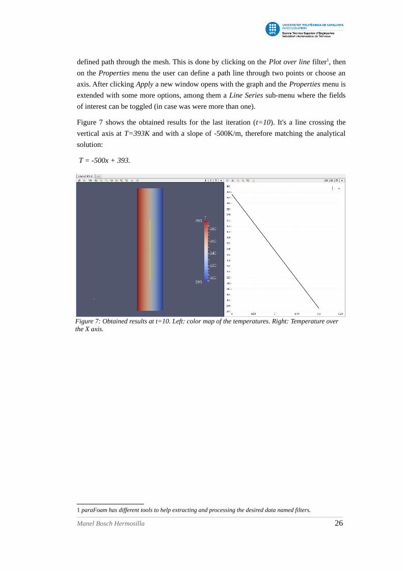
defined path through the mesh. This is done by clicking on the Plot over line filter1, then

on the Properties menu the user can define a path line through two points or choose an

axis. After clicking Apply a new window opens with the graph and the Properties menu is

extended with some more options, among them a Line Series sub-menu where the fields

of interest can be toggled (in case was were more than one).

Figure 7 shows the obtained results for the last iteration (t=10). It's a line crossing the

vertical axis at T=393K and with a slope of -500K/m, therefore matching the analytical

solution:

T = -500x + 393.

1 paraFoam has different tools to help extracting and processing the desired data named filters.


Figure 7: Obtained results at t=10. Left: color map of the temperatures. Right: Temperature over the X axis.

1.2 Part B: Transient conduction


This case maintains the dimensions, properties and boundaries of the previous one, except

for the right boundary which now has a time dependent temperature condition and

therefore its a transient problem. This new condition is described by:

T right = 293 + 20· sin(2π f ·t ) With f =1

86400

Which corresponds to a sinusoidal oscillation of 20K around 293K and with a period of

86400s (one day).

The initial condition is the steady-state solution at t = 0 (the solution of the previous

case).

1.2.1.1 Assumptions

• Top and bottom surfaces are adiabatic.

• Constant, uniform thermo-physical properties.

• One-dimensional conduction.

1.2.1.2 Formulation

Like in the previous case the governing equation is the heat equation but now the

temporal term isn't null:


Figure 8: schematic of the new problem

T = 293+sin(2πf·t)

L = 0.2 mH

= 1

mq = 500 W/m2

α = 5.8·10-7 m²/sκ = 1 W/(m·K)

∂T∂ t−α∇

2T = 0

Consequently the case can still be handled with the laplacianFoam solver.

1.2.2 Preprocessing

This case will be treated as a modification of the previous one. The mesh is kept the same

so the Polymesh contents can be reused, and the rest of files only have minor

modifications.

1.2.2.1 Boundary and initial conditions

In order to use the solution of the previous case as the initial condition of this one it's

enough to copy the T file from the last time-folder and place it in the 0 folder of this case.

The user can observe now the internal field is a list of the calculated values for each cell

and below there's the boundaryField sub-dictionary with the previous specification of

the boundary. Next is necessary to edit this to include the new boundary condition:

Note: To use the fields from a previous solution without special modifications the

mesh must remain the same.

1 boundaryField2 {3 left4 {5 type fixedGradient;6 gradient uniform 500;7 }8 right9 {10 type oscillatingFixedValue;11 refValue uniform 1; // Reference value for oscillation12 offset 292; // Oscillation mean value offset13 amplitude constant 20; // Amplitude of oscillation14 frequency constant 1.1574e-5; // frequency (1/86400)15 }16 TopBottom17 {18 type zeroGradient;19 }20 FrontBack21 {22 type empty;23 }24 }

The right face of the wall (right patch) now has a condition of the type

oscillatingFixedValue which is used to specify a condition of the kind:

refValue·(1+amplitude·sin (2π · frequency · t))+offset


Thus:

T right = 1 ·(1+20 ·sin (2π t

86400))+292 = 293+20 · sin(

2π t86400

)

1.2.2.2 Control and schemes

Finally the controlDict and fvSchemes dictionaries also need some modifications.

In fvSchemes a transient scheme has to be specified within ddtschemes. For this

example the Crank-Nicolson scheme is used. Next to the corresponding keyword there's

an off-centering coefficient which can weight the scheme from a pure implicit Euler

method (0) to pure Crank-Nicolson (1).

1 ddtSchemes2 {3 default CrankNicolson 1;4 }5

In controlDict some time parameters are modified to set a simulation time of two days

with a time-step of 360 seconds (which relative to the speed of the problem is small

enough to provide good time precision) and a write interval of an hour:

1 application laplacianFoam;23 startFrom startTime;45 startTime 0;67 stopAt endTime;89 endTime 172800;1011 deltaT 360;1213 writeControl runTime;1415 writeInterval 3600;1617 purgeWrite 0;1819 writeFormat ascii;2021 writePrecision 6;2223 writeCompression off;2425 timeFormat general;2627 timePrecision 6;2829 runTimeModifiable true;



After running laplacianFoam the results can be evaluated in the same way as the

precious problem. Since now the solution has a time dependence, with paraFoam the user

can navigate through the written results (every 3600s) to check the temperature

distribution at the given time, but the application has also some functions to plot data over

time which will be introduced next (see Figure 10 for a reference on the controls).

One way to plot the results over time is to directly select a cell on the 3D view with

Select Cells on (the selected cell will appear with a purple outline) and then click on Plot

Selection Over Time and Apply; a new window will appear with the corresponding chart

(the desired fields can be selected on the Properties menu). For example Figure 11 shows

the result for the right face, which naturally is the imposed boundary condition.


Figure 10: Reference for the described controls to plot the fields at a desired location.

Figure 9: Temperature distribution at t=43200s (12h)

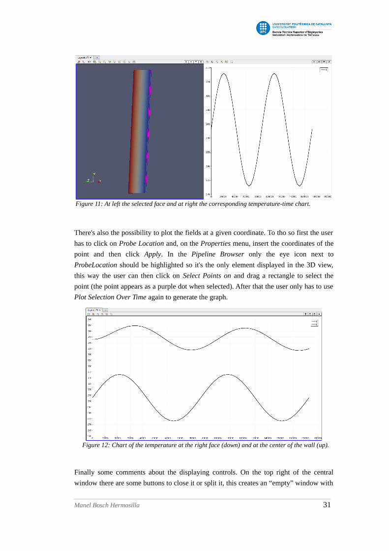
There's also the possibility to plot the fields at a given coordinate. To tho so first the user

has to click on Probe Location and, on the Properties menu, insert the coordinates of the

point and then click Apply. In the Pipeline Browser only the eye icon next to

ProbeLocation should be highlighted so it's the only element displayed in the 3D view,

this way the user can then click on Select Points on and drag a rectangle to select the

point (the point appears as a purple dot when selected). After that the user only has to use

Plot Selection Over Time again to generate the graph.

Finally some comments about the displaying controls. On the top right of the central

window there are some buttons to close it or split it, this creates an “empty” window with


Figure 12: Chart of the temperature at the right face (down) and at the center of the wall (up).

Figure 11: At left the selected face and at right the corresponding temperature-time chart.

a list of options. When having this empty window selected the eye icons on the Pipeline

Browser can be used to control what is displayed, be it a chart or a 3D entity. In a similar

way multiple graphs can be displayed at once (like in Figure 12) by having the chart

window selected and using the corresponding eye icons.


Chapter 2 - Multiple MaterialsThis chapter introduces the chtMultiRegionSimpleFoam (chtMRSF) solver for the

resolution of steady-state conduction problems involving different materials. This solver

uses a particular case structure which will be detailed here. chtMultiRegionSimpleFoam

also allows the solution of conjugate heat transfer problems (problems combining

conduction and convection) which will be explained in Chapter 4.

2.1 Description of the case

The model case consists on a 2D block formed by three different materials. The bottom of

the block is adiabatic, the top receives a constant inwards heat flux and each side is

exposed to a fluid with a known, constant, uniform temperature and heat transfer

coefficient. Figure 13 summarizes these boundary conditions and the geometry and the

thermal conductivity of each material is indicated in Table 2.

Material Thermal conductivity [W/(m² · K)]

A 0.5

B 210

C 2

Table 2: Thermal conductivities of the materials.


Figure 13: Schematic of the case.

2.1.1 Assumptions

• Bi-dimensional heat transfer

• Steady-state conditions

• Constant, uniform thermo-physical properties

• No contact resistance between materials

• Known heat transfer coefficients

• Negligible radiation exchange with surroundings.

2.1.2 Formulation

Like the previous chapter this is a conduction problem described by the heat equation and

the Fourier's Law, which with the proper simplifications are reduced to:

∂2 T∂ x2 +

∂2 T∂ y2 = 0

q⃗ =−κ(∂T∂ x

i⃗ +∂T∂ y

j⃗)

As for the convection heat transfer at the side walls, it is modeled according to the

Newton's law of cooling:

qout = h(T wall−T a)

But note that since the heat transfer coefficients (h) are assumed known this case isn't

really dealing with the convection problem (this will be done in the next chapter).

2.2 Preprocessing

Despite this case being very similar to the one in the first chapter its structure is quite

different because now there are three different regions, one for each material. The

laplacianFoam solver can't handle multiple regions without modifying the code, so this

problem will be solved with chtMultiRegionSimpleFoam, a steady-state solver which

can deal with processes involving heat transfer between different solids and between a

solid and a fluid (but again, the convection problem isn't resolved yet in this chapter).

Note: The transient version of chtMutiRegionSimpleFoam is chtMultiRegion-

Foam and it follows the same structure. “cht solvers” may be used to refer to

both.


The diagram below shows the new file structure of the case. The main difference with the

previous is that now there's a specific folder for every material, both in the constant and

system directories. These folders contain information or dictionaries specific to each

region and can be named however the user prefers to identify each region (remembering

that there should be no spaces). For this example they are leftSolid (material B),

rightSolid (material C) and topSolid (material A).

2.2.1 Mesh Generation

The meshing strategy is to create a single 2D mesh for the whole domain and then (after

specifying the boundary conditions) use the splitMeshRegions tool to divide it in the three

different regions. The mesh is generated using blockMesh with the following

blockMeshDict code:

1 convertToMeters 1;23 vertices4 (5 (0 0 -0.01)6 (0.9 0 -0.01)7 (0.9 0.5 -0.01)8 (0 0.5 -0.01)9 (0 0 0.01)10 (0.9 0 0.01)11 (0.9 0.5 0.01)12 (0 0.5 0.01)13 );1415 blocks16 (17 hex (0 1 2 3 4 5 6 7) (90 50 1) simpleGrading (1 1 1)18 );1920 edges21 (22 );2324 boundary25 (26 maxY27 {


3Solids ├── 0 │ ├── p │ └── T ├── constant │ ├── leftSolid │ │ ├── polyMesh │ │ └── thermophysicalProperties │ ├── polyMesh │ ├── rightSolid │ │ ├── polyMesh │ │ └── thermophysicalProperties │ ├── topSolid │ │ ├── polyMesh │ │ └── thermophysicalProperties │ └── regionProperties └── system │ :

: ├── leftSolid │ ├── changeDictionaryDict │ ├── fvSchemes │ └── fvSolution ├── rightSolid │ ├── changeDictionaryDict │ ├── fvSchemes │ └── fvSolution ├── topSolid │ ├── changeDictionaryDict │ ├── fvSchemes │ └── fvSolution ├── blockMeshDict ├── controlDict ├── fvSchemes ├── fvSolution └── topoSetDict

28 type wall;29 faces30 (31 (3 7 6 2)32 );33 }34 minX35 {36 type wall;37 faces38 (39 (0 4 7 3)40 );41 }42 maxX43 {44 type wall;45 faces46 (47 (2 6 5 1)48 );49 }50 minY51 {52 type wall;53 faces54 (55 (1 5 4 0)56 );57 }5859 );6061 mergePatchPairs62 (63 );6465 // ************************************************************************* //

Although the boundary faces could be a patch type, with the wall type the heat rates

across them can be quickly obtained with a built-in post-processing tool later. The front

and back faces (z-axis) are undefined so they are automatically assigned to the

defaultFaces group with an empty type.

2.2.2 Initial and boundary conditions

The boundary conditions are initially specified in the T file inside the 0 directory. Alse

there has to be p file because it is required by the thermophysicalProperties

dictionary although it doesn't have any physical meaning in this case.

T:

1 dimensions [0 0 0 1 0 0 0];23 internalField uniform 300;45 boundaryField6 {7 maxY8 {9 type externalWallHeatFluxTemperature;10 kappa solidThermo;11 q uniform 150;


12 value uniform 300.0;13 kappaName none;14 }15 minY16 {17 type zeroGradient;18 }19 minX20 {21 type externalWallHeatFluxTemperature;22 kappa solidThermo;23 Ta uniform 275;24 h uniform 5;25 value uniform 300.0;26 kappaName none;27 }28 maxX29 {30 type externalWallHeatFluxTemperature;31 kappa solidThermo;32 Ta uniform 473;33 h uniform 100;34 value uniform 300.0;35 kappaName none;36 }37 38 defaultFaces39 {40 type empty;41 }4243 }4445 // ************************************************************************* //

p:

1 dimensions [1 -1 -2 0 0 0 0];23 internalField uniform 1e5;45 boundaryField6 {7 ".*"8 {9 type calculated;10 }11 }

The externalWallHeatFluxTemperature type used in T can impose a fixed heat flux

condition by directly specifying it (q keyword, positive value for entering flux) or a fixed

heat transfer coefficient condition (i.e qout = h(T wall−T a) ) introducing the heat transfer

coefficient (h) and the ambient temperature (Ta) instead. Also this condition obtains the

thermal conductivity from the properties specified for each region and it only needs to be

told it's a solid material with solidThermo next to the kappa keyword. The value entry

is just the initial temperature value.

As for p, all patches (".*")2 are simply given a calculated type.

2 The “.*” is a “wildcard” character (i.e. it stands for any character) that can be used to apply a condition to any patch (“.*”), any patch whose name begins with certain string (“string.*”), etc.


2.2.3 Mesh splitting

In order to split the mesh with the splitMeshRegions tool the different regions of the mesh

have to be defined with the topoSet tool using the following topoSetDict dictionary:

1 actions2 (3 4 // leftSolid5 {6 name leftSolid; //name of the set7 type cellSet; 8 action new; //create a new set9 source boxToCell; //use a selection box10 sourceInfo11 {12 box (0 0 -1 )(0.6 0.25 1); //box corners13 }14 }15 {16 name leftSolid;17 type cellZoneSet;18 action new;19 source setToCellZone;20 sourceInfo21 {22 set leftSolid;23 }24 }2526 // rightSolid27 {28 name rightSolid;29 type cellSet;30 action new;31 source boxToCell;32 sourceInfo33 {34 box (0.6 0 -1 )(0.9 0.25 1);35 }36 }37 {38 name rightSolid;39 type cellZoneSet;40 action new;41 source setToCellZone;42 sourceInfo43 {44 set rightSolid;45 }46 }4748 // topSolid49 {50 name topSolid;51 type cellSet;52 action new;53 source boxToCell;54 sourceInfo55 {56 box (0 0.25 -1 )(0.9 0.5 1);57 }58 }59 {60 name topSolid;61 type cellZoneSet;62 action new;63 source setToCellZone;64 sourceInfo65 {66 set topSolid;


67 }68 }69 );7071 // ************************************************************************* //

The definition has two parts, the first one (lines 5 to 14) creates a cellSet using a

selection box which is defined by the coordinates of the two opposed corners, the box

doesn't need to match the domain as long as it contains only the desired part of the mesh.

Next (lines 15 to 24) a cellzone is created by using the previous cellSet as a source.

This is repeated for each region. With this topoSet will extract and store the necessary

information to divide the mesh into the corresponding regions after executing it by typing

in the terminal:

topoSet

After that typing:

splitMeshRegions -cellZones -overwrite

Will execute the splitMeshRegions tool which will divide the mesh according to the

specified cellZones and store the split meshes within the corresponding region-folder,

inside constant.

To view this divided meshes first is necessary to use the next command to prepare the

.OpenFOAM file of each region:

paraFoam -touchAll

And next the user can launch paraview to open them:

paraview

The regions are opened by clicking on Open, in the File menu, and selecting the

corresponding .OpenFOAM files. Multiple files can be selected to open them at once. After

that each region will appear in the pipeline browser and can be handled separately.


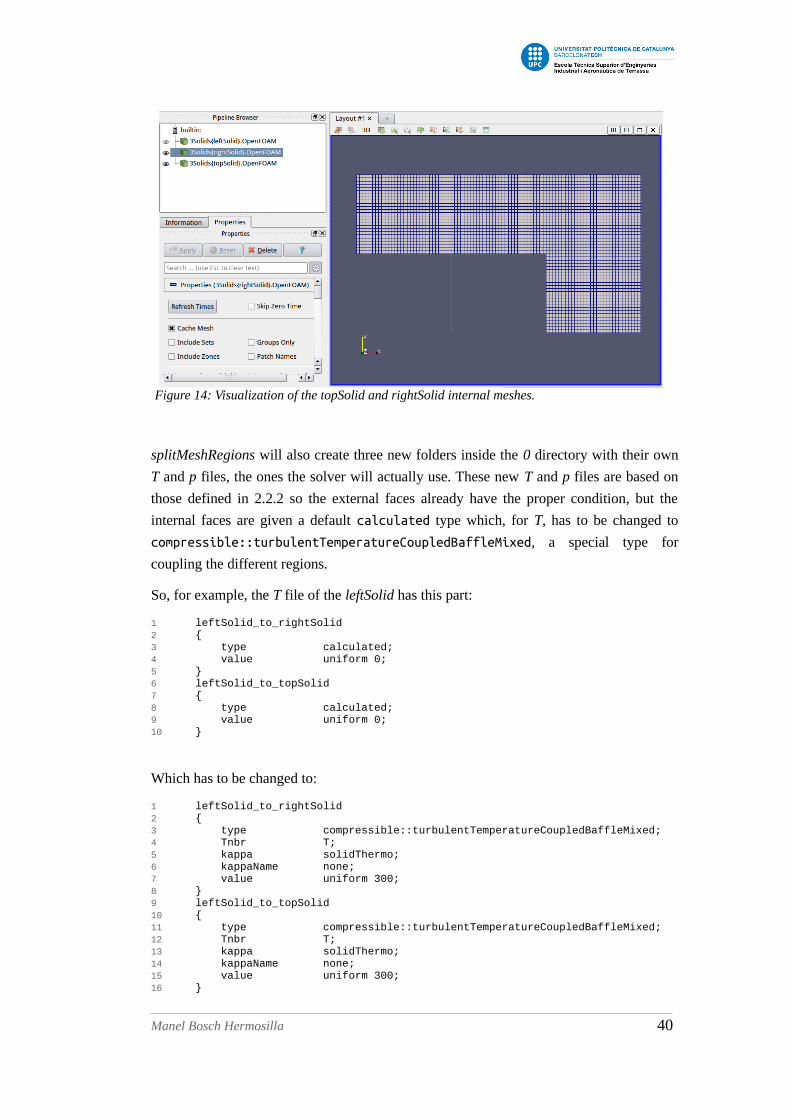
splitMeshRegions will also create three new folders inside the 0 directory with their own

T and p files, the ones the solver will actually use. These new T and p files are based on

those defined in 2.2.2 so the external faces already have the proper condition, but the

internal faces are given a default calculated type which, for T, has to be changed to

compressible::turbulentTemperatureCoupledBaffleMixed, a special type for

coupling the different regions.

So, for example, the T file of the leftSolid has this part:

1 leftSolid_to_rightSolid2 {3 type calculated;4 value uniform 0;5 }6 leftSolid_to_topSolid7 {8 type calculated;9 value uniform 0;10 }

Which has to be changed to:

1 leftSolid_to_rightSolid2 {3 type compressible::turbulentTemperatureCoupledBaffleMixed;4 Tnbr T;5 kappa solidThermo;6 kappaName none;7 value uniform 300;8 }9 leftSolid_to_topSolid10 {11 type compressible::turbulentTemperatureCoupledBaffleMixed;12 Tnbr T;13 kappa solidThermo;14 kappaName none;15 value uniform 300;16 }


Figure 14: Visualization of the topSolid and rightSolid internal meshes.

The same is repeated for the other regions.

There's a specific tool to replace entries and automatize this process, the

changeDictionary. It uses the changeDictionaryDict located in the corresponding

region-folder in system. For the leftSolid this dictionary should be:

1 dictionaryReplacement2 {3 T4 {5 boundaryField6 {7 "leftSolid_to.*"8 {9 type compressible::turbulentTemperatureCoupledBaffleMixed;10 Tnbr T;11 kappa solidThermo;12 kappaName none;13 value uniform 300;14 }15 }16 }17 }1819 // ************************************************************************* //

With this, after executing in the terminal:

changeDictionary -region leftSolid

The entries from the patches of the T file of the leftSolid whose name starts with

“leftSolid_to” will be replaced by the ones in the changeDictionaryDict.

It's possible to go further and make an script by creating a new text file (e.g. changeT) in

the case directory with:

1 #!/bin/sh23 for i in leftSolid rightSolid topSolid4 do5 changeDictionary -region $i 6 done

This way the changeDictionary of each region can be executed by simply launching the

file from the terminal:

bash changeT

2.2.4 Physical properties

The chtMRSF solver relies on the thermophysicalProperties dictionary which

establishes the material properties and the thermo-physical model.

The first part is common on the three regions, it sets a model for a solid material with

constant properties:


1 thermoType2 {3 type heSolidThermo;4 mixture pureMixture;5 transport constIso;6 thermo hConst;7 equationOfState rhoConst;8 specie specie;9 energy sensibleEnthalpy;10 }

The second part defines the thermal conductivity (kappa) of each material among other

unnecessary properties which are just placeholders, as they aren't relevant for the

governing equations of the case. E.g. for the leftSolid:

11 mixture12 {13 specie14 {15 nMoles 1;16 molWeight 12;17 }1819 transport20 {21 kappa 210; 22 }2324 thermodynamics25 {26 Hf 0;27 Cp 450;28 }2930 equationOfState31 {32 rho 8000;33 }34 }

Also within the constant directory there is a file named regionProperties which indicates

the solver the names of the solid and fluid regions to solve, both entries must be

present but as there aren't fluid regions this one is left void:

1 regions2 (3 fluid ()4 solid (leftSolid rightSolid topSolid)5 );67 // ************************************************************************* //

2.2.5 Control, solution and schemes

The three regions use the same fvSchemes and fvSolution inside the corresponding region

folder in system.


system/regionFolder/fvSchemes:

1 ddtSchemes2 {3 default steadyState;4 }56 gradSchemes7 {8 default Gauss linear;9 }1011 divSchemes12 {13 default none;14 }1516 laplacianSchemes17 {18 default none;19 laplacian(alpha,h) Gauss linear uncorrected;20 }2122 interpolationSchemes23 {24 default linear;25 }2627 snGradSchemes28 {29 default uncorrected;30 }3132 fluxRequired33 {34 default no;35 }3637 // ************************************************************************* //

system/regionFolder/fvSolution:

1 solvers2 {3 h4 {5 solver PCG;6 preconditioner DIC;7 tolerance 1e-06;8 relTol 0;9 }10 }1112 SIMPLE13 {14 nNonOrthogonalCorrectors 0;15 }161718 // ************************************************************************* //

Also to prevent errors the fvSolution and fvSchemes in the system directory are left there,

but they contain no information besides the header.


system/fvSolution:

1 FoamFile2 {3 version 2.0;4 format ascii;5 class dictionary;6 object fvSolution;7 }8 // * * * * * * * * * * * * * * * * * * * * * * * * * * * * * * * * * * * * * //910 // ************************************************************************* //

system/fcSchemes:

1 FoamFile2 {3 version 2.0;4 format ascii;5 class dictionary;6 object fvSchemes;7 }8 // * * * * * * * * * * * * * * * * * * * * * * * * * * * * * * * * * * * * * //910 ddtSchemes11 {12 }1314 gradSchemes15 {16 }1718 divSchemes19 {20 }2122 laplacianSchemes23 {24 }2526 interpolationSchemes27 {28 }2930 snGradSchemes31 {32 }3334 fluxRequired35 {36 }373839 // ************************************************************************* //

And last the controlDict is:

1 application chtMultiRegionSimpleFoam;23 startFrom startTime;45 startTime 0;67 stopAt endTime;89 endTime 500;1011 deltaT 1;


1213 writeControl timeStep;1415 writeInterval 100;1617 purgeWrite 10;1819 writeFormat ascii;2021 writePrecision 7;2223 writeCompression uncompressed;2425 timeFormat general;2627 timePrecision 6;2829 runTimeModifiable true;303132 // ************************************************************************* //

2.3 Running the simulation

First let's summarize all the commands used for the preprocessing:

blockMesh

topoSet

splitMeshRegions -cellZones -overwrite

changeDictionary -region leftSolid

changeDictionary -region rightSolid

changeDictionary -region topSolid

After the preprocessing is complete the simulation can begin with:

foamJob -screen chtMultiRegionSimpleFoam

2.4 Post-processing

Once the results are ready the user can launch paraview to visualize the results in the

same manner as the explained in 2.2.3 to visualize the mesh, remembering the .OpenFOAM

file of each region can be generated with the paraFoam -touchAll command, but it's not

necessary to repeat this step if the files are already present.

Once loaded in paraview each region is handled separately but they can be grouped by

selecting all of them (clicking on them while holding the Ctrl key) and using the Group

Datasets filter. Several GroupDatasets entities appear within the Pipeline Browser which

can be selected to handle all the regions as one (Figure 15), this is necessary to plot a

field over a line crossing multiple regions.

Before grouping it's important to note the Volume Fields and Mesh Parts the user wants to

load need to be selected individually first, from the Properties menu of each region, and


then click Apply.

Besides paraview there's another very useful post-processing tool for heat transfer

problems, that calculates the global heat rates (W) and the local heat fluxes (W/m²)

through the wall faces of a region, this can help confirming the convergence and

validating the results. It is executed by typing in the terminal:

wallHeatFlux -latestTime -region nameOfRegion

With this the terminal will output the boundary heat rates of the region “nameOfRegion”

for the solution stored in the last time-folder (if the latestTime argument is used). Also

inside the pertinent region-folder of this last time-folder a wallHeatFlux file is created

containing the normal heat flux at each boundary patch cell, which can be post-processed

with paraview as well.

The obtained heat rates are exposed in the next table:

Heat rate [W]

Face position [m] leftSolid rightSolid topSolid

X = 0 -152.5 / -87.37

X = 0.6 135.6 -135.7 /

X = 0.9 / 105.0 -0.1108

Y = 0 0.000 0.000 /

Y = 0.25 16.84 30.64 -47.52

Y = 0.5 / / 135.0

Σ -0.1 -0.1 0.0

Table 3: Heat rates through the boundary faces of each region. Positive values for a heat flux entering the region.


Figure 15: Group Datasets filter.

Overall the error is low which is a sign of good convergence and the results look

consistent with the physics of the case.

Note: Notice even though this is a 2D case the mesh is a 3D block and the total

heat rates are computed by integrating the heat fluxes over the finite area of the

mesh (for this reason the z-dimension of the mesh was conveniently set to 1m).

The average heat flux can be obtained by simply dividing the heat rate by this

area.

To conclude the chapter here are some other results from paraview.

Temperature distribution on the leftSolid (κ = 210W/(m·K)):

In Figure 17 the temperature distribution on the whole domain. The temperature of the

leftSolid may look constant but as Figure 16 showed that's because it has a much smaller

temperature gradient (because of the higher thermal conductivity) and so the small

temperature differences not appreciated due to the wider data range of this representation.


Figure 16: Temperature distribution on the leftSolid region (material 2)

Temperature vs. x-coordinate at the y=0.2m plane. Hence from x=0 to 0.6m it

corresponds to the leftSolid and from 0.6 to 0.9m the rightSolid. It highlights the

difference in temperature gradients.


Figure 17: Temperature distribution on the whole domain

Figure 18: Temperature [K] vs. x [m] across the y=0.2m plane.

Chapter 3 - ConvectionThis chapter explains the implementation of thermal convection for its resolution with

buoyantSimpleFoam and buoyantPimpleFoam, the steady-state and transient solvers for

compressible, convective flows. These solvers are chosen because they are the most

general and because they resolve the flow in the same way as the cht solvers, hence

together with Chapter 2 this chapter also establishes the base for the resolution of

conjugate heat transfer problems.

However the problems presented in this chapter could also be resolved with slight

modifications under the incompressible flow assumption with the Boussinesq

approximation using the buoyantBoussinesqSimpleFoam and buoyantBoussinesq-

PimpleFoam solvers.

The Part B of this chapter also introduces snappyHexMesh, a powerful meshing utility

very useful for meshing complex geometries.

3.1 Part A: Forced convection


This first part of the chapter will study the convective heat transfer for a case of external,

forced convection of dry air over an isothermal, horizontal, semi-infinite plate. Therefore

unlike the previous chapters now only the fluid domain will be resolved, with a boundary

conditioned by the plate.

Figure 19 shows the configuration of the problem. The plate has a length of 0.5m an it's

kept at constant 600K. The upstream flow has a velocity of 5m/s, a temperature of 300K

and a pressure of 101325Pa (1 atm). The thermo-physical properties of the fluid are

assumed constant and evaluated at the film temperature (450K), they are indicated in

Table 4.

cp [J/(kg·J)] μ [10-5 kg/(m·s)] κ [W/(m·K)] Pr

1028 2.484 0.03713 0.6878

Table 4: Thermo-physical properties of the fluid (dry air).


3.1.1.1 Assumptions


• Bi-dimensional, compressible, laminar flow

• Newtonian fluid

• Perfect gas

• Constant thermo-physical properties

• Negligible radiation effects

3.1.1.2 Formulation

The fundamental governing equations of the problem are the three conservation laws of

mass, momentum and energy.

Conservation of mass:

∂ρ

∂ t+ ∇⋅(ρ u⃗)= 0

Conservation of momentum:

ρD u⃗D t

= − ∇ · p + ∇ · τ⃗ + ρ · g⃗

Whre τ is the deviatoric stress tensor, for a compressible, Newtonian fluid this is:

τ ij=μ(∂u i

∂ x j

+∂u j

∂ x i

)−23μ∂uk

∂ xk

δij


Figure 19: Schematic of the problem.

And conservation of energy:

ρDhDt+ ρ

Dec

Dt=∂ p∂ t+ ∇ ·(κ∇ T ) + ρqv + ∇ ·( τ⃗ · u⃗) + ρ g⃗ ·u⃗

Where ec is the specific kinematic energy:

ec=12|⃗u|²

Since there aren't neither internal heat sources nor radiation interacting with the medium

the volumetric heat flux term, qv, is zero, and because it's a steady-state problem there's

no time dependence so the temporal derivatives are null as well. Hence the previous

equations can be simplified to:

∇⋅(ρ u⃗) = 0

ρ(u⃗ ·∇ u⃗)= − ∇ · p + ∇ · τ⃗ + ρ · g⃗

ρ(u⃗ ·∇ h+u⃗ ·∇ ec)=∂ p∂ t+ ∇ · (κ ∇ T ) + ∇ ·( τ⃗ ·u⃗ ) + ρ g⃗ · u⃗

And the perfect gas assumption provides this two additional relations:

pV = nRT h = c p T

Finally, the laminar to turbulent transition is characterized by the Reynolds number and it

happens around Rex = 5·10 , where the characteristic length is the traveled distance over⁵

the plate. For the proposed case the maximum Reynolds is:

ReL=ρU ∞ Lμ =

0.7846 ·5 ·0.52.484 ·10−5 = 78974

Which is still below the critical Reynolds so the assumption of laminar flow is consistent.


3.1.2 Preprocessing

Structure of the case:

3.1.2.1 Mesh Generation

The mesh is generated using blockMesh with the following blockMeshDict:

1 convertToMeters 1;23 vertices4 (5 (0 0 0)6 (0.5 0 0)7 (0.5 0.2 0)8 (0 0.2 0)9 (0 0 1)10 (0.5 0 1)11 (0.5 0.2 1)12 (0 0.2 1)13 );1415 blocks16 (17 hex (0 1 2 3 4 5 6 7) (100 100 1) 18 simpleGrading (1 40 1)19 );2021 edges22 (23 );2425 boundary26 (27 maxY28 {29 type symmetryPlane;30 faces31 (32 (3 7 6 2)33 );34 }35 inlet36 {37 type patch;38 faces


WallFlow ├── 0 │ ├── p │ ├── p_rgh │ ├── T │ └── U ├── constant │ ├── polyMesh │ ├── g │ ├── RASProperties │ ├── thermophysicalProperties │ └── turbulenceProperties └── system ├── blockMeshDict ├── controlDict ├── decomposeParDict ├── fvSchemes └── fvSolution

39 (40 (0 4 7 3)41 );42 }43 outlet44 {45 type patch;46 faces47 (48 (2 6 5 1)49 );50 }51 minY52 {53 type wall;54 faces55 (56 (1 5 4 0)57 );58 }59 );6061 mergePatchPairs62 (63 );6465 // ************************************************************************* //

The height of the domain is chosen so the upper patch is far enough from the developing

flow that a zeroGradient condition for the velocity can be considered physically

accurate and can be applied on that patch later.

Also this case takes advantage of the grading functionality, applying a grading of 40 on

the y-direction (thus 40 = [top cells height] / [bottom cells height]) to concentrate more

cells near the wall. Figure 20 and Figure 21 show the resulting mesh.


Figure 20: Visualization of the mesh.

Figure 21: Detail of the graded region.

3.1.2.2 Boundary conditions

This case uses four files for the initial boundary conditions: T (temperature), U (velocity)

and p (pressure) and p_rgh (pressure - ρgH) which is simply the pressure without the

hydrostatic contribution and simplifies the definition of the pressure boundaries.

T:

1 imensions [0 0 0 1 0 0 0];23 internalField uniform 300;45 boundaryField6 {7 maxY8 {9 type inletOutlet;10 inletValue uniform 300;11 value uniform 300;12 }13 inlet14 {15 type fixedValue;16 value uniform 300;17 }18 outlet19 {20 type zeroGradient;21 }22 minY23 {24 type fixedValue;25 value uniform 600;26 }2728 defaultFaces29 {30 type empty;31 }32 }3334 // ************************************************************************* //

U:

1 dimensions [0 1 -1 0 0 0 0];23 internalField uniform (5 0 0);45 boundaryField6 {7 maxY8 {9 type zeroGradient;10 }11 minY12 {13 type fixedValue;14 value uniform (0 0 0);15 }16 inlet17 {18 type fixedValue;19 value uniform (5 0 0);20 }21 outlet22 {23 type inletOutlet;


24 inletValue uniform (0 0 0);25 value uniform (5 0 0);26 }2728 defaultFaces29 {30 type empty;31 }32 }3334 // ************************************************************************* //

The boundary conditions of temperature and velocity on the inlet, and minY patches are

self-explanatory. Since U is a vector the corresponding values are defined by the three

components of the vector.

On the outlet the inletOutlet type is used for the velocity, this type works as a

fixedValue if the flow enters the domain (using the inletValue) and as a

zeroGradient if it exits it, in this case it is used to avoid reverse flow as it's not

expected, this can improve the stability of the resolution. On the maxY patch the velocity

uses zeroGradient as explained previously and the inletOutlet type is used for the

temperature, this is recommended for patches where it's unclear whether the flow will

enter or exit the domain or where both things can happen.

p_rgh:

1 dimensions [1 -1 -2 0 0 0 0];23 internalField uniform 101325;45 boundaryField6 {7 maxY8 {9 type fixedValue;10 value $internalField;11 }12 minY13 {14 type fixedFluxPressure;15 value $internalField;16 }17 inlet18 {19 type fixedFluxPressure;20 value $internalField;21 }22 outlet23 {24 type fixedValue;25 value $internalField;26 }2728 defaultFaces29 {30 type empty;31 }32 }3334 // ************************************************************************* //

p:


1 dimensions [1 -1 -2 0 0 0 0];23 internalField uniform 101325;45 boundaryField6 {7 ".*"8 {9 type calculated;10 value $internalField;11 }1213 defaultFaces14 {15 type empty;16 }17 }1819 // ************************************************************************* //

As for the pressure, since the pressure boundaries are defined through p_rgh, p is left as

calculated at all patches aside from those entirely defined by the geometric condition

(such as empty or symmetryPlane). With this, p is simply computed as p = p_rgh + ρgH

The field p_rgh uses a fixedFluxPressure type for the inlet and minY, this adjusts the

gradient according to the velocity at the boundary and is the usual type on patches where

the velocity is known. At the outlet and maxY the pressure is specified through a

fixedValue (101325).

These two files make use of the keyword $internalField for the value entries, this

instructs OpenFOAM to use the same value as the one specified in internalField

which can be a more convenient.

3.1.2.3 Properties

The thermo-physical properties are defined with the thermophysicalProperties dictionary

in a similar way as the previous chapter but using a model for a perfect gas with constant

properties:

1 thermoType2 {3 type heRhoThermo;4 mixture pureMixture;5 transport const; //constant mu and Pr6 thermo hConst; //constant Cp7 equationOfState perfectGas;8 specie specie;9 energy sensibleEnthalpy;10 }111213 mixture14 {15 specie16 {17 nMoles 1;18 molWeight 28.9;19 }20 thermodynamics


21 {22 Cp 1028.3;23 Hf 0;24 }25 transport26 {27 mu 2.484e-05;28 Pr 0.6878;29 }30 }

In addition there are two new dictionaries used for the determination of the turbulence

model which have to be set to laminar.

turbulenceProperties:

1 simulationType laminar;234 // ************************************************************************* //

RASProperties:

1 RASModel laminar;23 turbulence off;45 printCoeffs on;678 // ************************************************************************* //

Finally, the file named g determines the direction and magnitude of the gravitational

acceleration:

1 dimensions [0 1 -2 0 0 0 0];2 value ( 0 -9.81 0 );34 // ************************************************************************* //

3.1.2.4 Control, Solution and Schemes

fvSolution:

1 solvers2 {3 p_rgh4 {5 solver GAMG;6 tolerance 1e-7;7 relTol 0.01;89 smoother DICGaussSeidel;1011 cacheAgglomeration true;12 nCellsInCoarsestLevel 100;13 agglomerator faceAreaPair;14 mergeLevels 1;15 maxIter 100;16 }1718 "(U|h)"


19 {20 solver PBiCG;21 preconditioner DILU;22 tolerance 1e-7;23 relTol 0.01;24 }25 }2627 SIMPLE28 {29 momentumPredictor no;30 nNonOrthogonalCorrectors 0;31 pRefCell 0;32 pRefValue 0;333435 }3637 relaxationFactors38 {39 rho 1;40 p_rgh 0.7;41 U 0.7;42 h 0.7;43 }

fvSchemes:

1 ddtSchemes2 {3 default steadyState;4 }56 gradSchemes7 {8 default Gauss linear;9 }1011 divSchemes12 {13 default bounded Gauss upwind;14 div((muEff*dev2(T(grad(U))))) Gauss linear;15 }1617 laplacianSchemes18 {19 default Gauss linear uncorrected;20 }2122 interpolationSchemes23 {24 default linear;25 }2627 snGradSchemes28 {29 default uncorrected;30 }3132 fluxRequired33 {34 default no;35 p_rgh;36 }373839 // ************************************************************************* //

A very general guideline for the fvSchemes dictionary, when dealing with compressible


flows, is to begin the simulations with a first order (upwind) default scheme under

divSchemes, bounded for steady-state simulations and unbounded for transient, as higher

order schemes can cause stability issues.

controlDict:

1 application buoyantSimpleFoam;23 startFrom latestTime;45 startTime 0;67 stopAt endTime;89 endTime 1500;1011 deltaT 1;1213 writeControl runTime;1415 writeInterval 250;1617 purgeWrite 0;1819 writeFormat ascii;2021 writePrecision 9;2223 writeCompression off;2425 timeFormat general;2627 timePrecision 6;2829 runTimeModifiable true;3031 adjustTimeStep no;3233 maxCo 1;3435 // ************************************************************************* //

3.1.3 Running the simulation in parallel

OpenFOAM supports parallel processing by using the method known as domain

decomposition, this can significantly reduce the computation time when multiple

processors are available. With this method the domain is divided into several sub-

domains which can be allocated to different processors for solution. The process involves

the decomposition of the case, the resolution of the decomposed case and the posterior

recomposition in order to normally post-process the results.

To decompose it the decomposeParDict dictionary is needed to specify how the domain is

divided:

1 numberOfSubdomains 4;2 method simple;3 simpleCoeffs4 {5 n ( 2 2 1); //x y z6 delta 0.001;7 }8


9 distributed false;10 roots11 (12 );13 14 // ************************************************************************* //

In numberOfSubdomains the total number of sub-domains is specified. With the simple

method the domain is divided by direction into pieces with a similar number of cells, the

number of divisions in each direction is given at the n enty in line 5. delta is a parameter

known as cell skew factor, typically set to 10-3.

Next, to decompose the case the user has to run from the terminal:

decomposePar

After that several “processor-files” (processor0, processor1…) will appear within the case

directory, one for each sub-domain. This step has to be repeated every time the mesh or

the boundary conditions are modified. For this reason using the force argument can be

useful as this will automatically replace any preexisting processor file:

decomposePar -force

Now the case is ready to run in parallel, in order to begin the parallel execution in a local

machine the following command can be used:

foamJob -screen -parallel <name of the solver>

In this case:

foamJob -screen -parallel buoyantSimpleFoam

Lastly, after the computation has finished, the case can be reconstructed with the

command below, leaving it ready for a normal post-processing:

reconstructPar


This case can be validated by comparing the Nusselt number with the ones obtained

through empirical correlations found in the literature. For an isothermal horizontal plate

under a forced, laminar flow the following one is proposed in Fundamentals of Heat and

Mass Transfer (Incropera et al. 2011 [1]):

Nux = 0.664 · Rex(1 /2) · Pr (1/3 )

As for the Nusselt of the simulated case it can be obtained using wallHeatFlux since:

q̇ = h A (T w−T f )=NuL·κ

LA (T w−T f )


Where L is the total length of the plate and Tw-Tf the difference between the temperature

of the plate (Tw) and the temperature of the flow far from the plate (Tf).

The results are summarized in Table 5. The obtained Nusselt is a 10.53% greater than the

one of the correlation which, considering empirical correlations may not be very accurate,

is a good enough result to validate the case.

Simulation heat rate[W]

SimulationNuL

CorrelationNuL

Simulation/Correlation [%]

2028.0 182.06 164.72 10.53

Table 5: Comparison between the average Nusselt numbers obtained from the simulation and the empirical correlation.

To end, next are some more results post-processed with paraFoam using the basic tools

explained in the previous chapters.

Magnitude of the velocity of the flow. Close to the wall the laminar boundary layer starts

developing:

Temperature distribution near the wall at the right end. The thermal boundary layer can be

appreciated as well:


Figure 22: Magnitude of the velocity of the flow over the whole domain.

Temperature and velocity profiles near the wall at x=0.25m:


Figure 24: Temperature [K] vs. y [m] (up) and velocity [m/s] vs. y [m](down) at x=0.25m.

Figure 23: Detail of the temperature distribution close to the wall at the right end.

3.2 Part B: Natural convection


In this second part of the chapter a transient, bi-dimensional case of natural convection of

the air surrounding an isothermal, horizontal cylinder is presented.

The case consists on an horizontal cylinder with a wall temperature kept at a constant

500K, surrounded by an open volume of dry air at 1atm, initially quiescent and with a

uniform temperature of 300K. The schematic below summarizes it.

The thermo-physical properties, assumed constant, are evaluated at the film temperature

(400K). See Table 6.


1021 2.285 0.03368 0.6929

Table 6: Thermo-physical properties of the fluid.

3.2.1.1 Assumptions




• Newtonian fluid

• Perfect gas



3.2.1.2 Formulation

The governing equations are the same as in the previous part but since it's a transient case

now the time dependent terms can't be eliminated.

Conservation of mass, momentum and energy:

∂ρ

∂ t+ ∇⋅(ρ u⃗)= 0

ρD u⃗D t

= − ∇ · p + ∇ · τ⃗ + ρ · g⃗

ρDhDt+ ρ

Dec

Dt=∂ p∂ t+ ∇ ·(κ∇ T ) + ∇ · ( τ⃗ · u⃗) + ρ g⃗ · u⃗

And the ideal gas law with constant heat capacity, from the perfect gas assumption:

pV = nRT h = c p T

In addition, the steady-state solution of natural convection problems is characterized by

the Rayleigh number, in this case:

RaD =gβ(T w−T∞)D

3

να =9.81 ·2.5·10−3 ·200 ·0.033

2.589 ·10−5·3.737 ·10−5 = 1.369 ·105

According to Kuehn T and Goldstein R (as cited by S.K.S. Boetcher, 2014 [3]) for

Rayleigh numbers between 10 and 10 the flow forms a laminar boundary layer around⁴ ⁸

the cylinder, so the calculated Rayleigh confirms the laminar flow assumption is in

agreement. At higher Rayleigh numbers the flow becomes turbulent and at lower ones the

heat transfer is dominated by conduction.


3.2.2 Preprocessing


3.2.2.1 Mesh generation

This part will introduce snappyHexMesh, a powerful 3D meshing tool which can generate

meshes based on STL or OBJ geometry files. The input geometry has to be located in

constant/triSurface, in this case the cylinder.stl file, a 3D model of the central

cylinder.

Since snappyHexMesh works in the 3 dimensions it will generate unnecessary divisions

in the z-direction, this would slow the solution so another tool is used to correct that:

extrudeMesh. This tool can create a mesh by extruding a face of the prior mesh generated

with snappyHexMesh, hence by extruding one of the faces perpendicular to Z in the z-

direction an equivalent mesh without z-divisions can be obtained.

Before using snappyHexMesh it's first necessary to generate a background mesh covering

all the domain inside the air container. This is done as usual with blockMesh. The

blockMeshDict is:

1 convertToMeters 0.001;23 vertices4 (5 (-150 -150 0)6 (150 -150 0)7 (150 450 0)8 (-150 450 0)9 (-150 -150 10)10 (150 -150 10)11 (150 450 10)12 (-150 450 10)


hotCylinder ├── 0 │ ├── p │ ├── p_rgh │ ├── T │ └── U ├── constant │ ├── polyMesh │ ├── triSurface │ │ └── cylinder.stl │ ├── g │ ├── thermophysicalProperties │ └── turbulenceProperties └── system ├── blockMeshDict ├── controlDict ├── decomposeParDict ├── extrudeMeshDict ├── fvSchemes ├── fvSolution └── snappyHexMeshDict

13 );1415 blocks16 (17 hex (0 1 2 3 4 5 6 7) (75 150 1) simpleGrading (1 1 1)18 );1920 edges21 (22 );2324 boundary25 (26 Top27 {28 type patch;29 faces30 (31 (3 7 6 2)32 );33 }34 Bottom35 {36 type patch;37 faces38 (39 (1 5 4 0)40 );41 } 42 sides43 {44 type patch;45 faces46 (47 (2 6 5 1)48 (0 4 7 3)49 );50 }51 symFront52 {53 type empty;54 faces55 (56 (4 5 6 7)57 );58 }59 symBack60 {61 type empty;62 faces63 (64 (0 3 2 1)65 );66 }67 );6869 mergePatchPairs70 (71 );7273 // ************************************************************************* //

This time the front and back empty faces are in separated patches so one of them can later

be used for the extrusion.

Next let's see the instructions for snappyHexMesh in snappyHexMeshDict. Mastering

snappyHexMesh requires time and experience, it is a very complex dictionary with lots of

entries and only some of the basic features are going to be discussed in this guide,


1 castellatedMesh true;2 snap true;3 addLayers false;4

This first part controls the three steps involved in the generation of the mesh. The first

step refines the background hexahedra mesh according to some specifications and

discards the part which doesn't belong to the domain (the internal part of the cylinder in

this case). The second step morphs the mesh so the cells in contact with the geometry

match its surface. The last can be used to add layer of cells over a surface. Figure 26

illustrates this:

The code follows with:

5 geometry6 {7 cylinder.stl8 {9 type triSurfaceMesh;10 scale 0.001;11 name cylinder;12 }13 refinementBox 14 {15 type searchableBox; 16 min (-0.05 -0.1 -1);


Figure 26: Example of meshing steps. A - Background mesh. B - Castellated mesh. C - Snapped mesh. D - Added layers.

A B

C D

17 max ( 0.05 1 1); 18 }1920 };21

This part is used to indicate the STL file or files used for the refinement and the snapping.

Since the file is in meter units the scale is set to 0.001 to convert to millimeter units. name

defines the name of the corresponding boundary patch in the mesh.

In addition this section can be used to specify user-defined refinement regions, in this

example this feature is used to define a box around the cylinder and the area where the

plume is expected to further refine this region.

Next:

22 castellatedMeshControls23 {24 maxLocalCells 1000000;2526 maxGlobalCells 2000000;2728 minRefinementCells 10;2930 maxLoadUnbalance 0.10;3132 nCellsBetweenLevels 15;3334 features35 (36 );3738 refinementSurfaces39 {40 cylinder41 {42 level (4 4);4344 patchInfo45 {46 type wall;47 }48 }49 }5051 resolveFeatureAngle 30;5253 refinementRegions54 {55 refinementBox56 {57 mode inside;58 levels ((0.05 1));59 }60 }61 62 locationInMesh (0.052631 0.058706 0.001);6364 allowFreeStandingZoneFaces false;65 }

These are the instructions related to the castellatedMesh step. Lines 38 to 49 define the

surface based refinement, i.e. refinement based on the proximity to the geometry surface.


The refinement level is based on the background mesh, level 1 divides a background

hexahedron by two in every dimension (resulting in 8 smaller parts) and each subsequent

level does the same relative to the hexahedra of the previous level (Figure 27).

The minimum and maximum levels are specified next to the level keyword, the

maximum level (at right) can be used to further refine where the local curvature angle is

greater than resolveFeatureAngle but it can have a negative impact on the quality of

the mesh and for this particular case is pointless because of the constant curvature. Below

that, at patchInfo, the geometric type corresponding to the cylinder patch is specified.

Next, from line 53 to 60, there's the part related to the region-wise refinement. At mode it

can be instructed to refine inside or outside the defined region or to refine based on a

distance from the bounding surface. The first entry in levels is used to specify the

distance on for distance mode so it has no effect in this example, and the second entry

specifies the refinement level.

Finally, locationInMesh defines where the domain of interest is, either inside or outside

the input geometry (the cylinder), so the program knows whether to keep the mesh inside

or outside, thus a point outside the cylinder is defined. Furthermore the point must be

within the domain but outside any cell face (even after the refinement), for that reason it's

a good idea to add some random decimals to make it more unlikely for the point to be on

a face.

The remaining instructions control the snap step, the addLayers step and the quality of

the mesh. They are as follows:

66 snapControls67 {68 nSmoothPatch 3;6970 tolerance 2.0;7172 nSolveIter 30;73


Figure 27: Refinement levels. A: Level 0 (background). B: Level 1. C: Level 2.

74 nRelaxIter 5;7576 nFeatureSnapIter 10;7778 implicitFeatureSnap false;7980 explicitFeatureSnap true;8182 multiRegionFeatureSnap false;83 }848586 addLayersControls87 {88 relativeSizes true;8990 layers91 {9293 }9495 expansionRatio 2;9697 finalLayerThickness 0.5;9899 minThickness 0.001;100101 nGrow 0;102103 featureAngle 90;104105 slipFeatureAngle 30;106107 nRelaxIter 3;108109 nSmoothSurfaceNormals 1;110111 nSmoothNormals 3;112113 nSmoothThickness 10;114115 maxFaceThicknessRatio 0.5;116117 maxThicknessToMedialRatio 0.3;118119 minMedianAxisAngle 90;120121 nBufferCellsNoExtrude 0;122123 nLayerIter 50;124 }125126 meshQualityControls127 {128 maxNonOrtho 65;129130 maxBoundarySkewness 20;131132 maxInternalSkewness 4;133134 maxConcave 80;135136 minVol 1e-13;137138 minTetQuality 1e-30;139140 minArea -1;141142 minTwist 0.05;143144 minDeterminant 0.001;145146 minFaceWeight 0.05;


147148 minVolRatio 0.01;149150 minTriangleTwist -1;151152 nSmoothScale 4;153154 errorReduction 0.75;155 }156157158 // Advanced159160 mergeTolerance 1e-6;161162163 // ************************************************************************* //

The next step is to set up the extrudeMeshDict:

1 constructFrom patch;2 sourceCase "$FOAM_CASE";3 sourcePatches (symFront);45 exposedPatchName symBack;67 flipNormals false;89 extrudeModel linearNormal;1011 nLayers 1;1213 expansionRatio 1.0;1415 linearNormalCoeffs16 {17 thickness 1;18 }1920 mergeFaces false; 2122 mergeTol 0;

• constructFrom patch: Use a patch as a source for the extrusion

• sourceCase: The case where it will look for the specified patch. With

“$FOAM_CASE” it uses the case where the dictionary is located.

• sourcePatches: The name of the patches to extrude.

• exposedPatchName: The name of the patch opposed to the extruded one.

• extrudeModel linearNormal: Extrude in the direction normal to the patch.

• nLayers: Number of divisions in the extruded direction.

• thickness: Length of the extrusion.

Once blockMeshDict, snappyHexMeshDict and extrudeMeshDict are set up the mesh isready to be generated by executing:


blockMeshsnappyHexMesh -overwriteextrudeMesh

As always, it is recommended to check the mesh with checkMesh and paraFoam.

3.2.2.2 Initial and boundary conditions

Setting the proper boundary conditions for open natural convection cases can be a

delicate matter, a strategy used in this case is to place the boundary patches far from the

cylinder in order to minimize their effect around the cylinder. The upper patch leaves an

even more generous distance in order to let the thermal plume (i.e. the rising stream of

hot air) develop properly.

On the sides and Bottom patches totalPressure and pressureInletOutletVelocity

are used for p_rgh and U respectively. The first one establishes a constant total pressure

(p0) condition and the second is a velocity condition meant for patches where the

pressure is specified (if the flow enters the domain it derives the normal velocity from the

mass flux and otherwise it acts as a ZeroGradient). The Top patch will be crossed by the

plume so as to not disturb it fixedFluxPressure (p_rgh) and zeroGradient (U) are

used instead.

As for the temperature, on all these external patches it takes advantage of the flexibility of

the inletOutlet condition.

The boundary conditions on the cylinder wall are the usual ones.


Figure 28: Overview of the mesh (left) and detail of the mesh near the cylinder (right).

U:

1 dimensions [0 1 -1 0 0 0 0];23 internalField uniform (0 0 0);45 boundaryField6 {7 sides8 {9 type pressureInletOutletVelocity;10 value uniform (0 0 0);11 }1213 Top14 {15 type zeroGradient;16 }17 Bottom18 {19 type pressureInletOutletVelocity;20 value uniform (0 0 0);21 }22 cylinder23 {24 type fixedValue;25 value uniform (0 0 0);26 }2728 symFront29 {30 type empty;31 }32 symBack33 {34 type empty;35 }36 }3738 // ************************************************************************* //

p_rgh:

1 dimensions [1 -1 -2 0 0 0 0];23 internalField uniform 101325;45 boundaryField6 {7 sides8 {9 type totalPressure;10 p0 $internalField;11 U U;12 phi phi;13 rho rho;14 psi none;15 gamma 1.4;16 value $internalField;17 }18 Top19 {20 type fixedFluxPressure;21 value $internalField;22 }23 Bottom24 {25 type totalPressure;26 p0 $internalField;27 U U;28 phi phi;


29 rho rho;30 psi none;31 gamma 1.4;32 value $internalField;33 }3435 cylinder36 {37 type fixedFluxPressure;38 value $internalField;39 }4041 symFront42 {43 type empty;44 }45 symBack46 {47 type empty;48 }49 }5051 // ************************************************************************* //

T:

1 dimensions [0 0 0 1 0 0 0];23 internalField uniform 300;45 boundaryField6 {7 ".*"8 {9 type inletOutlet;10 inletValue uniform 300;11 }12 cylinder13 {14 type fixedValue;15 value uniform 500;16 }1718 symFront19 {20 type empty;21 }22 symBack23 {24 type empty;25 }26 }2728 // ************************************************************************* //

p:

1 dimensions [1 -1 -2 0 0 0 0];23 internalField uniform 101325;45 boundaryField6 {7 ".*"8 {9 type calculated;10 value $internalField;11 }12


13 symFront14 {15 type empty;16 }17 symBack18 {19 type empty;20 }21 }2223 // ************************************************************************* //

3.2.2.3 Properties

With the previous part as a reference the thermophysicalProperties dictionary is simply

updated with the new properties and the rest is kept the same.

thermophysicalProperties:

1 thermoType2 {3 type heRhoThermo;4 mixture pureMixture;5 transport const;6 thermo hConst;7 equationOfState perfectGas;8 specie specie;9 energy sensibleEnthalpy;10 }111213 mixture14 {15 specie16 {17 nMoles 1;18 molWeight 28.9;19 }20 thermodynamics21 {22 Cp 1021.1;23 Hf 0;24 }25 transport26 {27 mu 2.285e-05;28 Pr 0.6929;29 }30 }313233 // ************************************************************************* //

3.2.2.4 Control, solution and schemes

When numerically solving transient flows an important stability criterion is the Courant–

Friedrichs–Lewy (CFL) condition which establishes that for the solution to converge is

necessary that:

C = Δt∑i=1

n uxi

Δ x i

≤ Cmax


Where:

• C is known as the Courant number.

• uxi is the component of the velocity in the x i dimension.

• Δ t is the time interval.

• Δ x i is the length interval.

The value of Cmax depends on the methods used for the solution, for explicit methods it's

tipically 1. OpenFOAM uses implicit/semi-implicit methods which allow greater Cmax

values, nevertheless values of the order of 1 are advised to ensure the stability and

precision when solving unsteady flows.

The CFL condition puts a limitation on the selected time-step but the maximum Courant

number has to be estimated first. There's also the possibility to let the algorithm

automatically adjust the time-step by specifying the desired Cmax, a very useful feature.

This is done through the controlDict by setting yes on adjustTimeStep and

introducing the Cmax on maxCo (see below, lines 31 and 33).

controlDict:

1 application buoyantPimpleFoam;23 startFrom latestTime;45 startTime 0;67 stopAt endTime;89 endTime 5;1011 deltaT 1e-4;1213 writeControl adjustableRunTime;1415 writeInterval 0.1;1617 purgeWrite 0;1819 writeFormat ascii;2021 writePrecision 9;2223 writeCompression off;2425 timeFormat general;2627 timePrecision 6;2829 runTimeModifiable true;3031 adjustTimeStep yes;3233 maxCo 1;3435 // ************************************************************************* //


Since the time-step is variable the writeControl is set to adjustableRunTime mode, it

works in a similar way as runTime but it readjusts the time-step to make it exactly

coincide with the writeInterval (0.2 seconds of simulated time), while runTime would

write the result of the closest solved time.

The fvSchemes and fvSolution dictionaries also have some differences respect to the

previous part:

fvSchemes:

1 ddtSchemes2 {3 default Euler;4 }56 gradSchemes7 {8 default Gauss linear;9 }1011 divSchemes12 {13 default none;14 div(phi,U) Gauss upwind;15 div(phi,h) Gauss upwind;16 div(phi,K) Gauss linear;17 div((muEff*dev2(T(grad(U))))) Gauss linear;18 }1920 laplacianSchemes21 {22 default Gauss linear corrected;23 }2425 interpolationSchemes26 {27 default linear;28 }2930 snGradSchemes31 {32 default corrected;33 }3435 fluxRequired36 {37 default no;38 p_rgh;39 }404142 // ************************************************************************* //

fvSolution:

1 solvers2 {3 "rho.*"4 {5 solver PCG;6 preconditioner DIC;7 tolerance 0;8 relTol 0;9 }1011 p_rgh


12 {13 solver PCG;14 preconditioner DIC;15 tolerance 1e-8;16 relTol 0.01;17 }1819 p_rghFinal20 {21 $p_rgh;22 relTol 0;23 }2425 "(U|h)"26 {27 solver PBiCG;28 preconditioner DILU;29 tolerance 1e-6;30 relTol 0.1;31 }3233 "(U|h)Final"34 {35 $U;36 relTol 0;37 }38 }3940 PIMPLE41 {42 momentumPredictor yes;43 nOuterCorrectors 20; 44 nCorrectors 2;45 nNonOrthogonalCorrectors 1;46 residualControl 47 {48 "(U|h)"49 {50 tolerance 1e-4;51 relTol 0;52 }53 p_rgh54 {55 tolerance 1e-4;56 relTol 0;57 }58 }59 }


The decomposeParDict is the same as the previous part and in a similar manner the

parallel execution is performed with the commands:

decomposePar -force

foamJob -screen -parallel buoyantPimpleFoam

And then, to leave it ready for the post-processing:

reconstructPar



The average Nusselt is compared with the one obtained with Morgan's correlation based

on experimental data (as cited by S.K.S. Boetcher, 2014 [3]):

NuD = 0.48 ·RaD(1/4)

As shown in Table 7 there's good agreement between the simulation result and the

correlation with only a difference of a 7.31%.

Simulation heat rate[W]

SimulationNuD

CorrelationNuD

Simulation/Correlation [%]

209.67 9.9086 9.2328 7.31

Table 7: Comparison between the average Nusselt numbers from the simulation and Morgan's correlation.

Figure 29 displays the temperature distribution at different times. In a real case the rising

air becomes turbulent at some point but since this is a laminar flow simulation it doesn't,

yet the results relative to the heat transfer are good as it doesn't have a significant effect

on the flow around the cylinder.


Figure 29: Temperature distribution at different times (same scale on all).

A proper reproduction of this turbulent transition would require a very expensive direct

numerical simulation (DNS), with a grid fine enough to capture the eddies up to the

Kolmogorov microscales, or modeling the phenomenon partially/entirely through a

turbulence model (Large Eddy Simulation / Reynolds Averaged Simulation), which

reduces the computational effort at the expense of some accuracy, but it is still

unnecessary for a case like this.

Finally Figure 30 shows the streamlines at different times.

In order to visualize the streamlines with paraFoam first it's necessary to apply a Slice

filter to cut a slice normal to the z-direction and then use the Stream Tracer filter on this

Slice. Within Stream Tracer properties there's an option named Seed Type, here the user

can select High Resolution Line Source to place a line and trace the streamlines crossing

it. A more complete representation can be achieved by using several Stream Tracer filters

and placing the lines conveniently.


Figure 30: Streamlines at different times.

Chapter 4 - Conjugate Heat

TransferThis chapter is the practical application of the two precious ones into a conjugate heat

transfer problem involving solid and fluid regions using chtMultiRegionSimpleFoam. It

also introduces a way to model variable thermo-physical properties on the flow.

4.1 Description of the case

The case consists on an horizontal wall composed of two materials A and B with different

thermal conductivities (indicated in Table 8) with the top and bottom sides exposed to

forced, horizontal, external flows of dry air at different temperatures (see Figure 31 for

details). The left and right sides of the wall are considered adiabatic.

Material Thermal conductivity [W/(m² · K)]

A 1

B 200

Table 8: Thermal conductivities of the solid materials.



4.1.1 Assumptions

• Steady-state conditions


• Newtonian fluid

• Perfect gas

• The thermo-physical properties of the fluids are functions of the temperature

• The thermal conductivities of the solids are constant and uniform

• No contact resistance between solids


4.1.2 Formulation

The formulation of the problem is the same seen on previous cases. On one side there are

the conservation equations which, once simplified, are the same as in 3.1.1.2:

∇⋅(ρ u⃗) = 0

ρ(u⃗ ·∇ u⃗)= − ∇ · p + ∇ · τ⃗ + ρ · g⃗

ρ(u⃗ ·∇ h+u⃗ ·∇ ec)=∂ p∂ t+ ∇ · (κ ∇ T ) + ∇ ·( τ⃗ ·u⃗ ) + ρ g⃗ · u⃗

And on the other side the heat equation which for this case is reduced to:

∇2T = 0

The solver solves each region separately according to the applicable equations and

couples them with a boundary condition of equal heat flux through the surfaces of contact

( the turbulentTemperatureCoupledBaffleMixed).

As for the thermo-physical properties of air, now dependent on the temperature, they are

modeled using the following expressions:

c p= 1034.09−2.849 ·10−1 T+7.817 ·10−4 T 2−4.971 ·10−7T 3

+1.077 ·10−10 T 4

μ =1.458 ·10−6 T−1.5

T +110.4 (Sutherland's formula)

κ = μcv (1.32+1.77 Rair

cv

) (modified Eucken's model)


4.2 Preprocessing


4.2.1 Mesh generation

The mesh is generated with blockMesh using the next blockMeshDict:

1 convertToMeters 1;23 vertices4 (5 (0 -0.25 0)6 (0.5 -0.25 0)7 (0.5 0.25 0)8 (0 0.25 0)9 (0 -0.25 1)10 (0.5 -0.25 1)11 (0.5 0.25 1)12 (0 0.25 1)13 );1415 blocks16 (17 hex (0 1 2 3 4 5 6 7) (100 250 1) 18 simpleGrading 19 (5 20 (21 (0.23 100 0.02) 22 (0.04 50 1) 23 (0.23 100 50)24 ) 25 1)26 );2728 edges


chtWall ├── 0 │ ├── p │ ├── p_rgh │ ├── T │ └── U ├── constant │ ├── botAir │ │ ├── polyMesh │ │ ├── g │ │ ├── RASProperties │ │ ├── thermophysicalProperties │ │ └── turbulenceProperties │ ├── botWall │ │ ├── polyMesh │ │ └── thermophysicalProperties │ ├── polyMesh │ ├── topAir │ │ ├── polyMesh │ │ ├── g │ │ ├── RASProperties │ │ ├── thermophysicalProperties │ │ └── turbulenceProperties │ ├── topWall │ │ ├── polyMesh │ │ └── thermophysicalProperties │ └── regionProperties :

: └── system ├── botAir │ ├── changeDictionaryDict │ ├── decomposeParDict │ ├── fvSchemes │ └── fvSolution ├── botWall │ ├── changeDictionaryDict │ ├── decomposeParDict │ ├── fvSchemes │ └── fvSolution ├── topAir │ ├── changeDictionaryDict │ ├── decomposeParDict │ ├── fvSchemes │ └── fvSolution ├── topWall │ ├── changeDictionaryDict │ ├── decomposeParDict │ ├── fvSchemes │ └── fvSolution ├── blockMeshDict ├── controlDict ├── fvSchemes ├── fvSolution └── topoSetDict

29 (30 );3132 boundary33 (34 maxY35 {36 type patch;37 faces38 (39 (3 7 6 2)40 );41 }42 minX43 {44 type patch;45 faces46 (47 (0 4 7 3)48 );49 }50 maxX51 {52 type patch;53 faces54 (55 (2 6 5 1)56 );57 }58 minY59 {60 type patch;61 faces62 (63 (1 5 4 0)64 );65 }66 );6768 mergePatchPairs69 (70 );7172 // ************************************************************************* //

The approach is similar as the one used for the grid in 3.1.2.1 (convection over horizontal

plate case): using a graded grid on the flow regions to achieve a finer mesh near the wall.

This is achieved through the multi-grading feature of blockMesh, this feature is available

since OpenFOAM v2.4 and allows the definition of multiple graded zones along a

direction by replacing the corresponding expansion ratio. Each zone is defined by an

array with three variables, the first one defines the fraction of the total length the zone

occupies, the second the fraction of cells it has and the third specifies its grading.

In this blockMeshDict the expansion ratio corresponding to the y-direction has been

replaced by:

20 (21 (0.23 100 0.02) 22 (0.04 50 1) 23 (0.23 100 50)24 (

This means the first 23cm of the height contains 100 cells with a grading of 1/50 (the

mesh is refined towards the direction of y), the next 4cm (the wall) has 50 cells without

grading and the remaining 23cm contains the rest of the cells with a grading of 50 (the


mesh is coarsened towards the direction of y).

Note: Though the first two variables are fractions they are normalized

automatically (i.e. in the example 0.23 actually means a fraction of 0.23/

[0.23+0.04+0.23] of the total height) so they can be expressed the way the user

feels more convenient.

In addition a simple grading is used for the x-direction too because of the greater

gradients expected towards the inlet as the boundary layers start developing. Figure 32

and Figure 33 show the resulting mesh.


Figure 32: General view of the mesh (red lines differentiate the regions).

Finally the following topoSetDict sets the cellZones of the four regions into which the

splitMeshRegions tool will divide the mesh (from top to bottom: topAir, topWall,

botWall and botAir):

1 actions2 (3 4 // topAir5 {6 name topAir; //name of the set7 type cellSet; 8 action new; //create a new set9 source boxToCell; //use a selection box10 sourceInfo11 {12 box (0 0.02 0)(1 0.25 1); //box corners13 }14 }15 {16 name topAir;17 type cellZoneSet;18 action new;19 source setToCellZone; 20 sourceInfo21 {22 set topAir;23 }24 }2526 // botAir27 {28 name botAir;29 type cellSet;30 action new;31 source boxToCell;32 sourceInfo33 {34 box (0 -0.25 0)(1 -0.02 1);35 }36 }37 {38 name botAir;39 type cellZoneSet;40 action new;


Figure 33: Detail view of the mesh around the wall.

41 source setToCellZone;42 sourceInfo43 {44 set botAir;45 }46 }4748 // topWall49 {50 name topWall;51 type cellSet;52 action new;53 source boxToCell;54 sourceInfo55 {56 box (0 0 0)(1 0.02 1);57 }58 }59 {60 name topWall;61 type cellZoneSet;62 action new;63 source setToCellZone;64 sourceInfo65 {66 set topWall;67 }68 }69 // botWall70 {71 name botWall;72 type cellSet;73 action new;74 source boxToCell;75 sourceInfo76 {77 box (0 -0.02 0)(1 0 1);78 }79 }80 {81 name botWall;82 type cellZoneSet;83 action new;84 source setToCellZone;85 sourceInfo86 {87 set botWall;88 }89 }90 );9192 // ************************************************************************* //

4.2.2 Boundary conditions

The boundary conditions are specified almost entirely within the changeDictionaryDict

of each region. For this reason on all the files in the 0 directory, p, p_rgh, T and U; the

boundaryField is left as:

1 boundaryField2 {3 ".*"4 {5 type calculated;6 value $internalField;7 }89 defaultFaces10 {


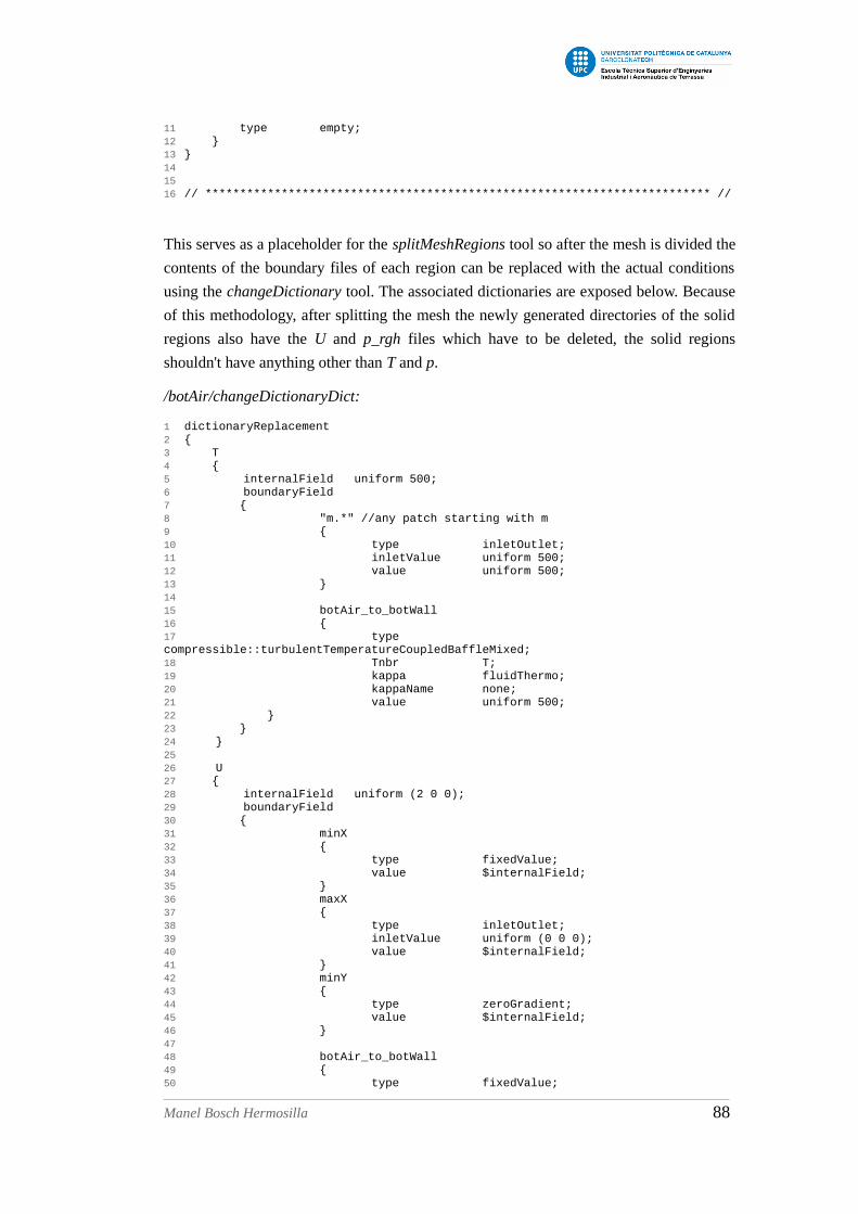
11 type empty;12 }13 }141516 // ************************************************************************* //

This serves as a placeholder for the splitMeshRegions tool so after the mesh is divided the

contents of the boundary files of each region can be replaced with the actual conditions

using the changeDictionary tool. The associated dictionaries are exposed below. Because

of this methodology, after splitting the mesh the newly generated directories of the solid

regions also have the U and p_rgh files which have to be deleted, the solid regions

shouldn't have anything other than T and p.

/botAir/changeDictionaryDict:

1 dictionaryReplacement2 {3 T4 {5 internalField uniform 500;6 boundaryField7 {8 "m.*" //any patch starting with m9 {10 type inletOutlet;11 inletValue uniform 500;12 value uniform 500;13 }1415 botAir_to_botWall16 {17 type compressible::turbulentTemperatureCoupledBaffleMixed;18 Tnbr T;19 kappa fluidThermo;20 kappaName none;21 value uniform 500;22 }23 }24 }2526 U27 {28 internalField uniform (2 0 0);29 boundaryField30 {31 minX32 {33 type fixedValue;34 value $internalField;35 }36 maxX37 {38 type inletOutlet;39 inletValue uniform (0 0 0);40 value $internalField;41 }42 minY43 {44 type zeroGradient;45 value $internalField;46 }4748 botAir_to_botWall49 {50 type fixedValue;


51 value uniform (0 0 0);52 }53 }54 }55 p_rgh56 {57 internalField uniform 1e5;58 boundaryField59 {60 minX61 {62 type fixedFluxPressure;63 value $internalField;64 }65 maxX66 {67 type fixedFluxPressure;68 value $internalField;69 }70 minY71 {72 type fixedValue;73 value $internalField;74 }75 botAir_to_botWall76 {77 type fixedFluxPressure;78 value $internalField;79 }80 }81 }82 83 }8485 // ************************************************************************* //

/topAir/changeDictionaryDict:

1 dictionaryReplacement2 {3 T4 {5 internalField uniform 293;6 boundaryField7 {8 "m.*"9 {10 type inletOutlet;11 inletValue uniform 293;12 value uniform 293;13 }1415 topAir_to_topWall16 {17 type compressible::turbulentTemperatureCoupledBaffleMixed;18 Tnbr T;19 kappa fluidThermo;20 kappaName none;21 value uniform 293;22 }23 }24 }2526 U27 {28 internalField uniform (1 0 0);29 boundaryField30 {31 minX32 {


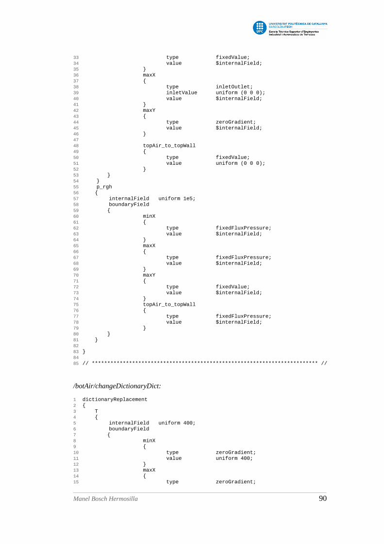
33 type fixedValue;34 value $internalField;35 }36 maxX37 {38 type inletOutlet;39 inletValue uniform (0 0 0);40 value $internalField;41 }42 maxY43 {44 type zeroGradient;45 value $internalField;46 }4748 topAir_to_topWall49 {50 type fixedValue;51 value uniform (0 0 0);52 }53 }54 }55 p_rgh56 {57 internalField uniform 1e5;58 boundaryField59 {60 minX61 {62 type fixedFluxPressure;63 value $internalField;64 }65 maxX66 {67 type fixedFluxPressure;68 value $internalField;69 }70 maxY71 {72 type fixedValue;73 value $internalField;74 }75 topAir_to_topWall76 {77 type fixedFluxPressure;78 value $internalField;79 }80 }81 } 82 83 }8485 // ************************************************************************* //


1 dictionaryReplacement2 {3 T4 {5 internalField uniform 400;6 boundaryField7 {8 minX9 {10 type zeroGradient;11 value uniform 400;12 }13 maxX14 {15 type zeroGradient;


16 value uniform 400;17 }18 botWall_to_topWall19 {20 type compressible::turbulentTemperatureCoupledBaffleMixed;21 Tnbr T;22 kappa solidThermo;23 kappaName none;24 value uniform 400;25 }26 botWall_to_botAir27 {28 type compressible::turbulentTemperatureCoupledBaffleMixed;29 Tnbr T;30 kappa solidThermo;31 kappaName none;32 value uniform 500;33 }34 }35 }3637 }3839 // ************************************************************************* //


1 dictionaryReplacement2 {3 T4 {5 internalField uniform 400;6 boundaryField7 {8 minX9 {10 type zeroGradient;11 value uniform 400;12 }13 maxX14 {15 type zeroGradient;16 value uniform 400;17 }18 topWall_to_topAir19 {20 type compressible::turbulentTemperatureCoupledBaffleMixed;21 Tnbr T;22 kappa solidThermo;23 kappaName none;24 value uniform 293;25 }26 topWall_to_botWall27 {28 type compressible::turbulentTemperatureCoupledBaffleMixed;29 Tnbr T;30 kappa solidThermo;31 kappaName none;32 value uniform 400;33 }34 }35 }3637 }3839 // ************************************************************************* //


The specific conditions combine what's seen in the chapters 2 and 3. Initially a

fixedPressure condition was used on the outlets but it was observed this can cause

convergence issues for low velocity flows and the fixedFluxPressure condition gives

better results.

4.2.3 Properties

This chapter introduces some guidelines on the specification of temperature-dependent

thermo-physical properties. To model that, this thermophysicalProperties dictionary is

used for both the topAir and botAir regions:

1 thermoType2 {3 type heRhoThermo;4 mixture pureMixture;5 transport sutherland;6 thermo hPolynomial;7 equationOfState perfectGas;8 specie specie;9 energy sensibleEnthalpy;10 }1112 mixture13 {14 specie15 {16 nMoles 1;17 molWeight 28.9;18 }19 thermodynamics20 {21 CpCoeffs<8> ( 1034.09 -2.849e-1 7.817e-4 -4.971e-7 1.077e-10 0 0 0);22 Hf 0;23 Sf 0;24 }25 transport26 {27 As 1.458e-06;28 Ts 110.4;29 }30 }313233 // ************************************************************************* //

First, within thermoType, the keywords transport sutherland and thermo

hPolynomial enables the use of the Sutherland/Eucken models and polynomial

expressions for the heat capacity.

With this, given a polynomial expression:

c p=∑i=0

7

ai Ti

The eight ai coefficients are introduced in the form of an ordered array after CpCoeffs<8>

(line 21).


And given the relation:

μ =A s · T−1.5

T +T s

The As and Ts coefficients are specified after the keywords As and Ts (lines 27, 28).

With these and the molar weight (molWeight) all the terms of the modified Eucken's

expression are determined so it doesn't need a particular entry.

This particular combination of models isn't part of the default pre-compiled set so it needs

to be compiled or otherwise it won't work. To do so it's only necessary to add the

following lines of code to the file /openfoam240/src/thermophysicalModels/basic/

rhoThermo/rhoThermos.C after the last makeThermo:

makeThermo( rhoThermo, heRhoThermo, pureMixture, sutherlandTransport, sensibleEnthalpy, hPolynomialThermo, perfectGas, specie);

And next open the terminal and run this two commands from within that same directory

(the directory were rhoThermos.C is):

sudo bash

wmake libso

Now that combination of models can be used.

The rest of properties files are as usual. RASProperties and turbulenceProperties are set

in laminar mode, the g files specify a downwards acceleration of 9,81m/s² and the

thermophysicalProperties of the solids simply specify the corresponding thermal

conductivities after the kappa keyword (remember since they're solids under steady-state

conditions only the other values aren't meaningful).

Finally regionProperties should look as follows:

1 regions2 (3 fluid (topAir botAir)4 solid (topWall botWall)5 );67 // ************************************************************************* //


4.2.4 Control, solution and schemes

controlDict:

1 application chtMultiRegionSimpleFoam;23 startFrom latestTime;45 startTime 0;67 stopAt endTime;89 endTime 6500;1011 deltaT 1;1213 writeControl timeStep;1415 writeInterval 500;1617 purgeWrite 0;1819 writeFormat ascii;2021 writePrecision 9;2223 writeCompression off;2425 timeFormat general;2627 timePrecision 6;2829 runTimeModifiable true;303132 // ************************************************************************* //

botAir and topAir fvSolution:

1 solvers2 {3 p_rgh4 {5 solver PCG;6 preconditioner DIC;7 tolerance 1e-9;8 relTol 0.01;9 }1011 "(U|h)"12 {13 solver PBiCG;14 preconditioner DILU;15 tolerance 1e-9;16 relTol 0.1;17 }18 }1920 SIMPLE21 {22 momentumPredictor no;23 nNonOrthogonalCorrectors 0;24 pRefCell 0;25 pRefValue 100000;26 rhoMin rhoMin [1 -3 0 0 0] 0.2;27 rhoMax rhoMax [1 -3 0 0 0] 2;2829 }3031 relaxationFactors32 {33 rho 1.0;34 p_rgh 0.7;35 U 0.7;


36 h 0.7;37 }3839 // ************************************************************************* //

botAir and topAir fvSchemes:

1 ddtSchemes2 {3 default steadyState;4 }56 gradSchemes7 {8 default Gauss linear;9 }1011 divSchemes12 {13 default bounded Gauss upwind;14 div((muEff*dev2(T(grad(U))))) Gauss linear;15 }1617 laplacianSchemes18 {19 default Gauss linear uncorrected;20 }2122 interpolationSchemes23 {24 default linear;25 }2627 snGradSchemes28 {29 default uncorrected;30 }3132 fluxRequired33 {34 default no;35 p_rgh;36 }373839 // ************************************************************************* //

botWall and topWall fvSolution:

1 solvers2 {3 h4 {5 solver PCG;6 preconditioner DIC;7 tolerance 1e-9;8 relTol 0.1;9 }10 }1112 SIMPLE13 {14 nNonOrthogonalCorrectors 0;15 }1617 relaxationFactors18 {19 h 1;20 }


212223 // ************************************************************************* //

botWall and topWall fvSchemes:

1 ddtSchemes2 {3 default steadyState;4 }56 gradSchemes7 {8 default Gauss linear;9 }1011 divSchemes12 {13 default none;14 }1516 laplacianSchemes17 {18 default none;19 laplacian(alpha,h) Gauss linear uncorrected;20 }2122 interpolationSchemes23 {24 default linear;25 }2627 snGradSchemes28 {29 default uncorrected;30 }3132 fluxRequired33 {34 default no;35 }3637 // ************************************************************************* //

4.3 Running the simulation in parallel

As the cases grow in complexity taking advantage of the linux bash scripting becomes

more useful. The post-precessing phase can be completed with the next script:

1 #!/bin/bash23 blockMesh4 topoSet5 splitMeshRegions -cellZones -overwrite67 rm ./0/topWall/{p_rgh,U}8 rm ./0/botWall/{p_rgh,U}910 for i in topAir botAir topWall botWall11 do12 changeDictionary -region $i > log.changeDictionary.$i 2>&113 done


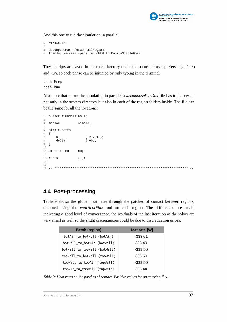
And this one to run the simulation in parallel:

1 #!/bin/sh23 decomposePar -force -allRegions4 foamJob -screen -parallel chtMultiRegionSimpleFoam

These scripts are saved in the case directory under the name the user prefers, e.g. Prep

and Run, so each phase can be initiated by only typing in the terminal:

bash Prep

bash Run

Also note that to run the simulation in parallel a decomposeParDict file has to be present

not only in the system directory but also in each of the region folders inside. The file can

be the same for all the locations:

1 numberOfSubdomains 4;23 method simple;45 simpleCoeffs6 {7 n ( 2 2 1 );8 delta 0.001;9 }1011 distributed no;1213 roots ( );141516 // ************************************************************************* //

4.4 Post-processing

Table 9 shows the global heat rates through the patches of contact between regions,

obtained using the wallHeatFlux tool on each region. The differences are small,

indicating a good level of convergence, the residuals of the last iteration of the solver are

very small as well so the slight discrepancies could be due to discretization errors.

Patch (region) Heat rate [W]

botAir_to_botWall (botAir) -333.61

botWall_to_botAir (botWall) 333.49

botWall_to_topWall (botWall) -333.50

topWall_to_botWall (topWall) 333.50

topWall_to_topAir (topWall) -333.50

topAir_to_topWall (topWair) 333.44

Table 9: Heat rates on the patches of contact. Positive values for an entering flux.


To end, some more results are shown with the next figures.

Temperature distribution with a custom coloring to better appreciate the gradients within

the wall:

Temperature profile near the wall at x=0.4m. The result is as expected, the flows near the

wall form a thermal boundary layer and the wall has differentiated temperature gradients

due to the different conductivities:


Figure 35: Temperature [K] vs. y [m] at x = 0.4m

Figure 34: Temperature distribution.

Chapter 5 - RadiationTo conclude this guide the fifth chapter explains the implementation of surface-to-surface

radiation with non-participating media. The used solvers are buoyantSimpleFoam and

chtMulti-RegionSimpleFoam which have already been exposed in previous chapters so

this one focuses on the radiation part.

Part B also explains the introduction of heat sources and develops a complete case of

conduction, convection and radiation with heat sources.

5.1 Part A: Convection + Radiation


The case consists of a square, bi-dimensional enclosure filled with dry air whose top and

bottom walls are adiabatic and the side walls are isothermal, with the left one having a

higher temperature than the right. All the walls have an emissivity ε = 0.8. The rest of

details are shown in Figure 36. This case is based on the numerical study of Wang et al.

(2006) [11], which studies this problem under the Boussinesq approximation.

The thermo-physical properties are defined as the properties of the dry-air evaluated at T 0

= 293.5K (Table 10).


1011 1.8151 0.02576 0.7124

Table 10: Thermo-physical properties of the fluid.



5.1.1.1 Assumptions



• Newtonian fluid

• Perfect gas


• Surface-to-surface radiation with non-participating medium

• The internal walls are gray, diffuse, opaque surfaces with a constant, uniform

emissivity

5.1.2 Formulation

This case has the same governing equations as 3.1.1.2 with the addition of a radiation

model. The Rayleigh number is:

RaL=gβ(T h−T c)L

3

να = 105

Because the medium is non-participating the radiation only affects the boundaries through

the surface-to-surface radiation exchange and since two of the walls haven't a fixed

temperature there's an interaction with the convection mode.

The radiation model of the simulation is based on the “radiosity method”. The method

relies on the last two of the listed assumptions which allow the radiosity (radiant energy

abandoning a surface, represented as J) and the irradiation (incidental radiant energy,

represented as G) of a surface k to be calculated as:

J k= εkσT 4+(1−ε)G k

Gk=∑i=1

N

Fki J i

Where the view factors, Fki, depend on the

geometry and are defined as:

Fki=kAk∫A k

∫Ai

cosθk cosθi

πS2 dA k dA i


Figure 37: Differential areas for view factors calculation [13].

Finally the definition of net radiative heat flux depends on the sign criteria. OpenFOAM

uses positive values for a flux entering the surface, therefore:

q rad,k=G k−J k

5.1.3 Preprocessing


5.1.3.1 Mesh Generation

A simple 120x120 grid is used for this case. The mesh is generated with blockMesh as

usual, using the next blockMeshDict:

1 convertToMeters 1;23 vertices4 (5 (0 0 0)6 (0.045 0 0)7 (0.045 0.045 0)8 (0 0.045 0)9 (0 0 1)10 (0.045 0 1)11 (0.045 0.045 1)12 (0 0.045 1)13 );1415 blocks16 (17 hex (0 1 2 3 4 5 6 7) (120 120 1) simpleGrading (1 1 1)18 );1920 edges21 (22 );


radCavity ├── 0 │ ├── p │ ├── p_rgh │ ├── Qr │ ├── T │ └── U ├── constant │ ├── polyMesh │ ├── g │ ├── radiationProperties │ ├── thermophysicalProperties │ ├── turbulenceProperties │ └── viewFactorsDict └── system ├── blockMeshDict ├── controlDict ├── decomposeParDict ├── fvSchemes └── fvSolution

2324 boundary25 (26 maxY27 {28 type wall;29 faces30 (31 (3 7 6 2)32 );33 }34 minX35 {36 type wall;37 faces38 (39 (0 4 7 3)40 );41 }42 maxX43 {44 type wall;45 faces46 (47 (2 6 5 1)48 );49 }50 minY51 {52 type wall;53 faces54 (55 (1 5 4 0)56 );57 }58 );5960 mergePatchPairs61 (62 );6364 // ************************************************************************* //

5.1.3.2 Boundary conditions

The inclusion of the radiation in the problem implies a new file named Qr which is the

field corresponding to the radiative heat flux and is used to define the related conditions.

Qr:

1 dimensions [1 0 -3 0 0 0 0];23 internalField uniform 0;45 boundaryField6 {7 minX8 {9 type greyDiffusiveRadiationViewFactor;10 emissivityMode lookup;11 Qro uniform 0;12 emissivity uniform 0.8;13 value uniform 0;14 }15 maxX16 {17 type greyDiffusiveRadiationViewFactor;18 emissivityMode lookup;19 Qro uniform 0;


20 emissivity uniform 0.8;21 value uniform 0;22 }23 minY24 {25 type greyDiffusiveRadiationViewFactor;26 emissivityMode lookup;27 Qro uniform 0;28 emissivity uniform 0.8;29 value uniform 0;30 }31 maxY32 {33 type greyDiffusiveRadiationViewFactor;34 emissivityMode lookup;35 Qro uniform 0;36 emissivity uniform 0.8;37 value uniform 0;38 }39 defaultFaces40 {41 type empty;42 }43 }4445 // ************************************************************************* //

The condition type associated with the radiosity method is the

greyDiffusiveRadiationViewFactor and hence it has to be used on every patch. The

emissivityMode is set to either lookup for a direct specification of the emissivity of

the wall or to solidRadiation to get the value from the properties of the solid region

which only applies to multi-region problems. This condition also requires the definition

of the external radiative heat flux, Qro, which in this case is 0 on all the patches.

T:

1 dimensions [0 0 0 1 0 0 0];23 internalField uniform 293.5;45 boundaryField6 {7 minX8 {9 type fixedValue;10 value uniform 298.5;11 }12 maxX13 {14 type fixedValue;15 value uniform 288.5;16 }17 minY18 {19 type compressible::turbulentHeatFluxTemperature;20 heatSource flux; // power [W]; flux [W/m2]21 q uniform 0; // heat power or flux22 kappaName none;23 kappa fluidThermo; // obtains kappa from thermo model24 Qr Qr; // name of the radiative flux25 value $internalField; // initial temperature value26 }27 maxY28 {29 type compressible::turbulentHeatFluxTemperature;30 heatSource flux; 31 q uniform 0;


32 kappaName none;33 kappa fluidThermo;34 Qr Qr; 35 value $internalField; 36 }37 defaultFaces38 {39 type empty;40 }4142 }4344 // ************************************************************************* //

The T file also use a new type of condition required to satisfy the restriction the adiabatic

walls impose on the internal faces which has the form:

−qrad+qconv,in=−qrad±κ(∇ T ) = 0

i.e. the sum of the radiative flux leaving the internal face (therefore entering the domain)

and the inwards convective flux equals 0.

Consequently turbulentHeatFluxTemperature is the proper type for these adiabatic

walls because it allows the definition of the total entering heat flux while taking into

account the radiative flux, respecting the aforementioned restriction.

The rest of condition files doesn't need any particular commentary.

U:

1 dimensions [0 1 -1 0 0 0 0];23 internalField uniform (0 0 0);45 boundaryField6 {7 ".*"8 {9 type fixedValue;10 value uniform (0 0 0);11 }12 defaultFaces13 {14 type empty;15 }16 }171819 // ************************************************************************* //

p:

1 dimensions [1 -1 -2 0 0 0 0];23 internalField uniform 103800;45 boundaryField6 {7 ".*"8 {9 type calculated;10 value $internalField;11 }


1213 defaultFaces14 {15 type empty;16 }17 }181920 // ************************************************************************* //

p_rgh:

1 dimensions [1 -1 -2 0 0 0 0];23 internalField uniform 103800;45 boundaryField6 {7 ".*"8 {9 type fixedFluxPressure;10 value $internalField;11 }12 defaultFaces13 {14 type empty;15 }16 }171819 // ************************************************************************* //

5.1.3.3 Properties

Another two new files related with the radiation modeling are located in the constant

directory: radiationProperties and viewFactorsDict.

radiationProperties in this case is used only to define the radiation model as the medium

doesn't participate with the radiation and the related parameters are defined through the

boundary conditions. The viewFactor model is the model corresponding to the described

radiosity method. Other possible models which won't be described in this work are the P1

(for optically thick media) or the fvDOM (finite volume discrete ordinates model, the most

versatile and computationally expensive of the three).

1 radiation on;23 radiationModel viewFactor;45 viewFactorCoeffs6 {7 smoothing true; //Smooth view factor matrix (use when in a close surface8 //to force Sum(Fij = 1)9 constantEmissivity true; //constant emissivity on surfaces.10 }1112 // Number of flow iterations per radiation iteration13 solverFreq 3;1415 absorptionEmissionModel none;161718 scatterModel none;19


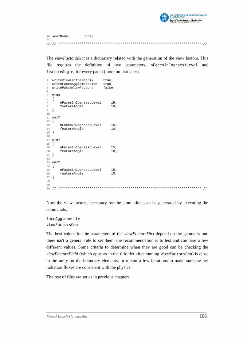
20 sootModel none;2122 // ************************************************************************* //

The viewFactorsDict is a dictionary related with the generation of the view factors. This

file requires the definition of two parameters, nFacesInCoarsestLevel and

featureAngle, for every patch (more on that later).

1 writeViewFactorMatrix true;2 writeFacesAgglomeration true;3 writePatchViewFactors false;45 minX6 {7 nFacesInCoarsestLevel 15;8 featureAngle 10;9 }1011 maxX12 {13 nFacesInCoarsestLevel 15;14 featureAngle 10;15 } 1617 minY18 {19 nFacesInCoarsestLevel 15;20 featureAngle 10;21 }22 23 maxY24 {25 nFacesInCoarsestLevel 15;26 featureAngle 10;27 }282930 // ************************************************************************* //

Now the view factors, necessary for the simulation, can be generated by executing the

commands:

faceAgglomerate

viewFactorsGen

The best values for the parameters of the viewFactorsDict depend on the geometry and

there isn't a general rule to set them, the recommendation is to test and compare a few

different values. Some criteria to determine when they are good can be checking the

viewFactorsField (which appears in the 0 folder after running viewFactorsGen) is close

to the unity on the boundary elements, or to run a few iterations to make sure the net

radiation fluxes are consistent with the physics.

The rest of files are set as in previous chapters.


5.1.3.4 Control, solution and schemes

controlDict:

1 application buoyantSimpleFoam;23 startFrom latestTime;45 startTime 0;67 stopAt endTime;89 endTime 5000;1011 deltaT 1;1213 writeControl timeStep;1415 writeInterval 500;1617 purgeWrite 0;1819 writeFormat ascii;2021 writePrecision 9;2223 writeCompression off;2425 timeFormat general;2627 timePrecision 6;2829 runTimeModifiable true;303132 // ************************************************************************* //

fvSolution:

1 solvers2 {3 rho4 {5 solver PCG;6 preconditioner DIC;7 tolerance 1e-7;8 relTol 0.1;9 }1011 p_rgh12 {13 solver PCG;14 preconditioner DIC;15 tolerance 1e-7;16 relTol 0.1;17 }1819 "(U|h)"20 {21 solver PBiCG;22 preconditioner DILU;23 tolerance 1e-7;24 relTol 0.1;25 }262728 }2930 SIMPLE31 {


32 momentumPredictor off;33 nNonOrthogonalCorrectors 0;34 pRefCell 0;35 pRefValue 0;36 }3738 relaxationFactors39 {40 fields41 {42 rho 1.0;43 p_rgh 0.7;44 }45 equations46 {47 U 0.7;48 h 0.7;49 Qr 0.7;50 }51 }5253 // ************************************************************************* //

fvSchemes:

1 ddtSchemes2 {3 default steadyState;4 }56 gradSchemes7 {8 default Gauss linear;9 }1011 divSchemes12 {13 default none;14 div(phi,U) bounded Gauss upwind;15 div(phi,K) bounded Gauss upwind;16 div(phi,h) bounded Gauss upwind;17 div((muEff*dev2(T(grad(U))))) Gauss linear;18 }1920 laplacianSchemes21 {22 default Gauss linear uncorrected;23 }2425 interpolationSchemes26 {27 default linear;28 }2930 snGradSchemes31 {32 default uncorrected;33 }3435 fluxRequired36 {37 default no;38 p_rgh;39 }4041 // ************************************************************************* //



The aforementioned faceAgglomerate and viewFactorsGen commands correspond to

the serial execution, the run the simulation in parallel the next commands have to be used

after preparing the preprocessing files and generating the mesh:

decomposePar -force

mpirun -np 4 faceAgglomerate -parallel

mpirun -np 4 viewFactorsGen -parallel

foamJob -screen -parallel buoyantSimpleFoam


This time the global heat rates will be analyzed with paraFoam and compared with the

results of Wang et al. [11] for a same Rayleigh and wall emissivities to validate the

results.

To do so, before launching paraFoam, is necessary to run the wallHeatFlux utility as in

previous problems to generate the field of the conductive/convective heat fluxes (named

wallHeatFlux as well). The field of the radiative heat fluxes is already present as Qr.

Next the user can open the case with paraFoam. Before clicking Apply he should make

sure that the Qr and wallHeatFlux fields are selected in the properties menu, as well as

the patch or patches of interest (and anything else), e.g. minX. Then an Integrate

Variables filter can be applied which will integrate Qr and wallHeatFlux over the surface

of the selected patches, therefore obtaining the global heat rates which are displayed in a

table (see Figure 38). Keep in mind that they use an opposite sign criteria as Qr is the

radiative flux entering the patch (opposite to internal face normal) and wallHeatFlux the

flux entering the domain (same direction as the internal face normal).


Figure 38: Using the Integrate Variables filter of paraFoam on the minX patch.

With this the radiative, convective and total (the sum of the two) Nusselt numbers can be

calculated for the comparison with Wang's work. The results are presented in Table 11

showing a good agreement.

This work Wang et al.

Nuc Nur Nut Nuc Nur Nut

Hot wall 4.211 5.081 9.292 4.189 5.196 9.385

Cold wall 4.273 5.021 9.294 4.247 5.137 9.384

Table 11: Obtained Nusselt numbers on hot and cold walls and comparison with Wang's results.

Finally the next figures show a representation of the isotherms and the streamlines. The

simplest method for the representation of isosurfaces in a 2D plane is to simply reduce

the Number Of Table Values in the Color Map Editor (marked in red in Figure 39).

Representation of the isotherms:


Figure 39: Isotherms.

Representation of the streamlines:


Figure 40: Streamlines.

5.2 Part B

5.2.1 Description of the problem

This case is a modification of a previous one where a heat generating solid, square block

has been placed in the center (Figure 41). The heat generation is considered uniform all

over the block and produces a total heat rate of 1W. The thermal conductivity of the solid

material is κ = 0.5 W/(K·m) and the thermal emissivity is ε = 0.8 on all the surfaces. The

rest of parameters and properties are the same as in the previous case.

5.2.1.1 Assumptions



• Newtonian fluid

• Perfect gas


• Surface-to-surface radiation with non-participating medium

• All the surfaces are gray, diffuse and opaque with a constant, uniform emissivity

• Uniform heat generation inside the block



5.2.1.2 Formulation

The formulation relative to the air region and the radiation is the same as in the previous

part, as for the solid the only change is the addition of the heat source term the the heat

equation:

ρc p∂T∂ t− κ∇

2T = qv

Which for a steady-state case is:

− κ∇2 T = qv

The chtMultiRegionSimpleFoam solver solves this in terms of enthalpy which will be

useful to keep in mind later, when the source term is being added:

− κc p

∇2h = qv

5.2.2 Preprocessing

This case uses the same mesh as the previous one, as well as the same external boundary

conditions and the same properties for the Air region, therefore most of the files are the

same but adapted to the file structure of the cht solvers which has already been detailed in

previous chapters, therefore this section won't go into as much detail.


radCavityWblock ├── 0 │ ├── p │ ├── p_rgh │ ├── T │ └── U ├── constant │ ├── Air │ │ ├── polyMesh │ │ ├── g │ │ ├── radiationProperties │ │ ├── RASProperties │ │ ├── thermophysicalProperties │ │ ├ ── turbulenceProperties │ │ └── viewFactorsDict │ ├── Solid │ │ ├── polyMesh │ │ ├── radiationProperties │ │ └── thermophysicalProperties │ ├── polyMesh │ └── regionProperties :

: └── system ├── Air │ ├── changeDictionaryDict │ ├── decomposeParDict │ ├── fvSchemes │ └── fvSolution ├── Solid │ ├── changeDictionaryDict │ ├── decomposeParDict │ ├── fvOptions │ ├── fvSchemes │ └── fvSolution ├── blockMeshDict ├── controlDict ├── decomposeParDict ├── fvSchemes ├── fvSolution └── topoSetDict

5.2.2.1 Boundary conditions and properties

As mentioned earlier the external boundary conditions are the same and as for the internal

ones, i.e. the conditions on the patches where the two regions meet, they are introduced

through the following changeDictionaryDict files:

/Air/changeDictionaryDict:

1 dictionaryReplacement2 {3 Qr4 {5 boundaryField6 {7 Air_to_Solid8 {9 type greyDiffusiveRadiationViewFactor;10 emissivityMode solidRadiation;11 Qro uniform 0;12 value uniform 0;;13 }14 }15 }1617 p_rgh18 {19 boundaryField20 {21 Air_to_Solid22 {23 type fixedFluxPressure;24 value $internalField;25 }26 }27 }2829 T30 {31 boundaryField32 {33 Air_to_Solid34 {35 type

compressible::turbulentTemperatureRadCoupledMixed;36 Tnbr T;37 kappa fluidThermo;38 QrNbr none;39 Qr Qr;40 kappaName none;41 value $internalField;42 }43 }44 }45 U46 {47 boundaryField48 {49 Air_to_Solid50 {51 type fixedValue;52 value uniform (0 0 0);53 }54 }55 }56 }575859 // ************************************************************************* //


/Solid/changeDictionaryDict:

1 dictionaryReplacement2 {3 T4 {5 boundaryField6 {7 Solid_to_Air8 {9 type

compressible::turbulentTemperatureRadCoupledMixed;10 Tnbr T;11 kappa solidThermo;12 QrNbr Qr;13 Qr none;14 kappaName none;15 value $internalField;16 }17 }18 }19 }2021 // ************************************************************************* //

The Qr field for the Air_to_Solid patch provides an example of the solidRadiation

emissivityMode which will get the emissivity from the radiationProperties file of the

solid region (exposed below), but it is still possible to just specify the emissivity directly

with the lookup mode.

1 radiation on;23 radiationModel opaqueSolid;45 absorptionEmissionModel constantAbsorptionEmission;67 constantAbsorptionEmissionCoeffs8 {9 absorptivity absorptivity [ 0 -1 0 0 0 0 0 ] 0.8; 10 emissivity emissivity [ 0 -1 0 0 0 0 0 ] 0.8;11 E E [ 1 -1 -3 0 0 0 0 ] 0;12 }1314 scatterModel none;1516 sootModel none;1718 // ************************************************************************* //

5.2.2.2 Adding the source term

The addition of the source term for the heat generation is done through the fvOptions

file inside the /system/Solid directory. fvOptions is a flexible framework that allows the

user to add different types of sources or constraints to the governing equations. This

section explains the scalarSemiImplicitSource type which permits the addition of any

source term of the kind S (X )=Su+S p X

In order to make sure fvOptions is being properly used first is necessary to understand

how OpenFOAM implements the governing equations, looking at the source code files

can provide some clues on that (/openfoam240/applications/solvers/heatTransfer/


chtMultiRegionFoam/solid/solveSolid.H).

As commented in 5.2.1.2 the cMRSF solver solves the heat equation in terms of enthalpy

so when using the SemiImplicitSource the equation becomes:

− κc p

∇2h = S(h) = Su+Sp h

Hence:

Su+S p h = qv → Su=qv , Sp=0

The corresponding fvOptions file will be:

1 HeatSource2 {3 type scalarSemiImplicitSource;4 active true;5 selectionMode all; 6 //cellZone cellZoneName;78 scalarSemiImplicitSourceCoeffs 9 {10 volumeMode absolute; //alt. specific11 injectionRateSuSp 12 {13 h (1 0);14 }15 }16 }1718 // ************************************************************************* //

fvOptions needs a definition of the region where the source term is applied, since in this

case this is the whole Solid region it's only necessary to set the selectionMode to all.

Another useful selectionMode is the cellZone one, with this the region is defied

through a cellZone created with topoSet whose name is indicated below after a

cellZone keyword (exemplified in line 6).

volumeMode allows the user to set whether the source is indicated as an absolute quantity

(absolute) or a quantity per unit of volume (specific).

Finally within injectionRateSuSp the Su and Sp coefficients are indicated after the name

of the field of the corresponding equation (h). In this case since the absolute mode is used

this means Su=qv ·V=1W (so there's no need to care about the volume).


5.2.3 Running the case in parallel

As in Chapter 4 a script like this can be used to run the post-processing utilities:

1 #!/bin/bash23 blockMesh4 topoSet5 splitMeshRegions -cellZones -overwrite67 rm ./0/Solid/{p_rgh,U,Qr}89 for i in Air Solid10 do11 changeDictionary -region $i > log.changeDictionary.$i 2>&112 done

And this one to begin the simulation. Notice the faceAgglomerate and viewFactorsGen

need additional arguments for a multi-region case.

1 #!/bin/sh23 decomposePar -force -allRegions4 mpirun -np 4 faceAgglomerate -region Air -parallel -dict constant/viewFactorsDict5 mpirun -np 4 viewFactorsGen -region Air -parallel6 foamJob -screen -parallel chtMultiRegionSimpleFoam


The controlDict was set to run for 8500 iterations and the following results were

obtained.

Global heat rates:

Heat rate [W]

Patch (region) Conv./Cond. Radiation Total

Solid_to_Air (Solid) -1.000 / -1.000

Air_to_Solid (Air) 0.5098 0.4902 1.000

MinX (Air) 0.7688 0.9307 1.700

MaxX (Air) -1.370 -1.331 -2.701

Table 12: Heat rates through different patches. Positive values for entering heat.


Isotherms:

Streamlines:


Figure 42: Isotherms.

Figure 43: Streamlines.



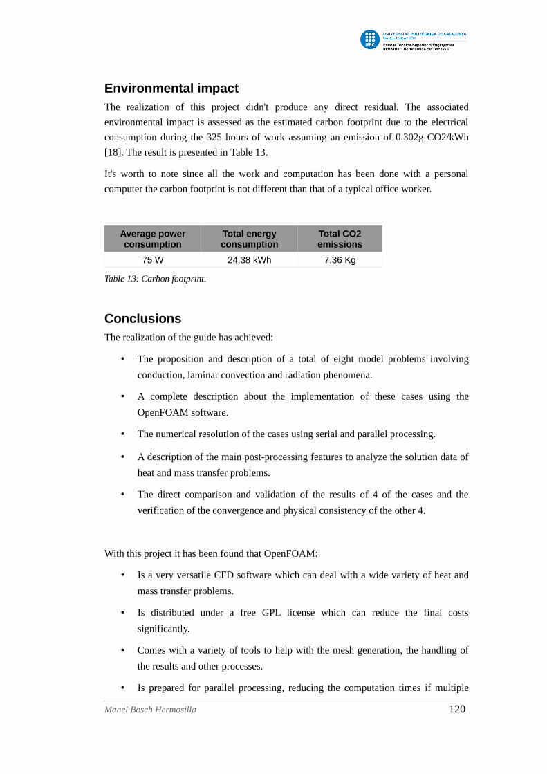
Environmental impactThe realization of this project didn't produce any direct residual. The associated

environmental impact is assessed as the estimated carbon footprint due to the electrical

consumption during the 325 hours of work assuming an emission of 0.302g CO2/kWh

[18]. The result is presented in Table 13.

It's worth to note since all the work and computation has been done with a personal

computer the carbon footprint is not different than that of a typical office worker.

Average powerconsumption

Total energyconsumption

Total CO2emissions

75 W 24.38 kWh 7.36 Kg

Table 13: Carbon footprint.

Conclusions The realization of the guide has achieved:

• The proposition and description of a total of eight model problems involving

conduction, laminar convection and radiation phenomena.

• A complete description about the implementation of these cases using the

OpenFOAM software.

• The numerical resolution of the cases using serial and parallel processing.

• A description of the main post-processing features to analyze the solution data of

heat and mass transfer problems.

• The direct comparison and validation of the results of 4 of the cases and the

verification of the convergence and physical consistency of the other 4.

With this project it has been found that OpenFOAM:

• Is a very versatile CFD software which can deal with a wide variety of heat and

mass transfer problems.

• Is distributed under a free GPL license which can reduce the final costs

significantly.

• Comes with a variety of tools to help with the mesh generation, the handling of

the results and other processes.

• Is prepared for parallel processing, reducing the computation times if multiple


processors are available.

• Is not an intuitive software. The data entry is generally handled with data

dictionaries and the utilities are executed through commands.

• Provides reliable results, provided the case is properly modeled.

Furthermore, as a personal conclusion, the research work for the elaboration of the guide

has brought me a lot of new knowledge about OpenFOAM, which I consider very

valuable as it has direct practical applications in the field of engineering; and the

elaboration itself further contributed to my self-development helping me better establish

both the newly acquired and the some of previous knowledge.

Further workFurther lines of work after this project could be the:

• Deeper description of the presented meshing utilities, particularly

snappyHexMesh.

• Study of the main numerical schemes and algorithms.

• Detailed analysis and description of the P1 and fvDOM radiation models. Use on

advanced radiation problems with participating media.

• Modeling of the turbulence. Description of the principal models, range of

applicability and considerations, application in thermal problems, comparison

with experimental or DNS data…

• Simulation of multi-phase flows with phase-change heat transfer.

• Combustion modeling. This may require the inclusion of the previous

phenomena.


Bibliography

[1] F. P. Incropera, D. P. DeWitt, T. L. Bergman, and A. S. Lavine, Fundamentals of

Heat and Mass Transfer, vol. 7th. John Wiley & Sons, 2007.

[2] J. D. Anderson, J. Degroote, G. Degrez, E. Dick, R. Grundmann, and J.

Vierendeels, Computational Fluid Dynamics: An Introduction, 2009.

[3] S. K. S. Boetcher, Natural Convection from Circular Cylinders, Springer, 2014.

[4] F. M. White, Viscous Fluid Flow, McGraw-Hill, vol. Second, p. 413, 2000.

[5] C. J. Greenshields, OpenFOAM, the open source CFD toolbox User Guide,

OpenFOAM Foundation, 2015

[6] J. Casacuberta, Study of fluid dynamics applications in the field of engineering

by using OpenFOAM, Universitat Politècnica de Catalunya, 2014.

[7] E. Agnani, snappyWiki, https://sites.google.com/site/snappywiki/, 2016.

[8] A. Singhal, Tutorial to set up a case for chtMultiRegionFoam in OpenFOAM

2.0.0, University of Luxembourg, 2014.

[9] M. Van Der Tempel, A chtMultiRegionSimpleFoam tutorial, Chalmers

University of Technology, 2012.

[10] A. Vdovin, Radiation heat transfer in OpenFOAM, Chalmers University of

Technology, 2009.

[11] H. Wang, S. Xin, and P. Le Quéré, Étude numérique du couplage de la

convection naturelle avec le rayonnement de surfaces en cavité carrée remplie

d’air, C.R. Mecanique, vol. 334, no. 1, pp. 48–57, 2006.

[12] Centre Tecnològic de Transferència de Calor, Formulario para la realización de

ejercicios de transferencia de calor y masa, Universitat Politècnica de

Catalunya.

[13] C.D.Pérez-Segarra, J.Castro, A.Oliva, R.Capdevila, Apunts de Transferència de

Calor per Radiació i Exercicis, Universitat Politècnica de Catalunya, 2013.

[14] CFD Direct, About OpenFOAM, http://cfd.direct/openfoam/about/, 2016.

[15] OpenCFD website, http://www.openfoam.com/, 2016.

[16] CFDsupport website, http://www.cfdsupport.com/, 2016.

[17] CFD Online, CFD-wiki, http://www.cfd-online.com/Wiki/Main_Page, 2016.


http://www.cfd-online.com/Wiki/Main_Page

http://www.cfdsupport.com/

http://www.openfoam.com/

http://cfd.direct/openfoam/about/

https://sites.google.com/site/snappywiki/

[18] Oficina catalana del cambio climatico, Nota informativa sobre la metodologia

de estimación del mix elèctrico por parte de la oficina catalana del cambio

climàtico, 2016.


Documents

Study of heat and mass transfer applications in the field