Embed Size (px)
Citation preview

STUDY OF FORCE DISCRIMINATION ON CHIRAL MOLECULES AND
PARTICLES BY CIRCULAR POLARIZED LIGHT AND METASURFACE
ENHANCED FIELD
BY
HANYANG ZHAO
THESIS
Submitted in partial fulfillment of the requirements
for the degree of Master of Science in Mechanical Engineering
in the Graduate College of the
University of Illinois at Urbana-Champaign, 2016
Urbana, Illinois
Advisor:
Professor Kimani C. Toussaint

ii
ABSTRACT
This thesis aims to explore force discrimination on chiral particles and molecules, when
experiencing an electromagnetic field. This thesis focuses especially on incident fields with
handedness. These fields come from incident circular polarized light or from enhanced
fields generated by a plasmonic metasurface. This topic was first motivated by the need of
separating enantiomers mechanically. Now many works have been done by different
groups. Inspired by these works, a general expression of force under an incident time-
varying electromagnetic field is derived in this thesis. Some of the recent works is reviewed
and discussed. This thesis also talks about the development of an open source near field
simulation tool. Many simulations were done and summarized here, along with a
discussion of the results.

iii
TABLE OF CONTENT
CHAPTER 1: INTRODUCTION ........................................................................................................... 1
1.1. Motivation .............................................................................................................................. 1
1.2. Circular dichroism and circular birefringence ........................................................................ 2
1.3. Conventional ways to separate chiral molecules .................................................................... 3
1.4. Optical force and Optical tweezer .......................................................................................... 4
1.5. Plasmonic metasurface optical trapping ................................................................................. 6
1.6. Figures .................................................................................................................................... 9
CHAPTER 2: THEORY AND FORCE EXPRESSION ....................................................................... 14
2.1. General model of chiral molecules ....................................................................................... 14
2.2. Electric polarizability and Clausius-Mossotti relation ......................................................... 15
2.3. The correction of Clausius-Mossotti relation due to chirality .............................................. 16
2.4. Optical force on dipoles ....................................................................................................... 18
2.5. The expansion of the force expression ................................................................................. 20
CHAPTER 3: LITERATURE REVIEW ............................................................................................... 23
3.1. Chiral near fields .................................................................................................................. 23
3.2. Discriminative force and optical trapping ............................................................................ 24
3.3. Related experiments ............................................................................................................. 27
3.4. Figures .................................................................................................................................. 29
CHAPTER 4: EXPERIMENTS AND SIMULATIONS ....................................................................... 33
4.1. DDA introduction ................................................................................................................. 33
4.2. nanoDDSCAT+ .................................................................................................................... 34
4.3. comparison of nanoDDSCAT+ and other software .............................................................. 36
4.4. data processing for force calculation .................................................................................... 36
4.5. Spiral structure simulation .................................................................................................... 37
4.6. Figures .................................................................................................................................. 39
CHAPTER 5: DISCUSSION AND CONCLUSION ............................................................................ 43
REFERENCES ..................................................................................................................................... 44

1
CHAPTER 1: INTRODUCTION
1.1. Motivation
Chiral molecules are molecules that have same composition but are mirror images to each
other. This property is called chirality or handedness and often happens when a carbon
atom is attached to four different substituents. This is due to the 3D structure of carbon
atom and its four covalent bonds. Chiral molecules widely exist in nature. For example, 19
of the 20 common amino acids that form proteins are chiral. These enantiomers can have
different effects on living body, so studying them is important to chemistry, biology and
pharmacy.
For example, many drugs have chirality, but when being synthesized both enantiomers are
produced in the ratio of one to one. Only the molecules with certain chirality have effect
on human body and the other halves are usually useless or even toxic to human body.
Therefore, pharmaceutical industry is really interested in how to synthesize the half they
want or how to separate them after synthesis.
Our motivation is to find a method to separate large chiral molecules using plasmonic
metasurface enhanced nearfield. This method can be extremely useful and may have great
potential in chemical and pharmaceutical industry.

2
1.2. Circular dichroism and circular birefringence
The fundamental assumption of this thesis is that chiral particles and chiral molecules will
interact with circular polarized light. The proof of this interaction lies in two phenomena
called circular dichroism and circular birefringence. The macro level change of circular
polarized light indicates the micro interaction between them.
A linear polarized light is an electromagnetic wave whose electric field or magnetic field
oscillate in a confine plane alone propagation. Circular polarized light (CPL) can be seen
as a superposition of two linear polarized light with same wavelength propagating in the
same direction with perpendicular polarization, these two linear polarized light also have a
π/2 phase difference so the maximum of the electric field is always the same but circulating
in a clockwise of counter-clockwise mode.
As a CPL can be seen as two linear polarized light, a linear polarized light can also be seen
as a superposition of one right CPL and another left CPL with no phase difference. When
a linear polarized light propagate through a birefringence material, one of the CPL will
travel slower than the other one. This will cause a phase difference between the two, thus
the superposition of the two, the linear polarized light, will change its direction of
polarization. This difference in propagation speed of CPL is called circular birefringence
and the change of polarize direction when a linear polarized light going through the
material is called an optical rotation.

3
Unlike circular birefringence, circular dichroism (CD) only happens when chiral molecules
absorb CPL at a different rate. As a result, an incoming linear polarized light will become
an elliptically polarized light since one of the CPL in the linear polarized light will have
lower intensity than the other one. A detailed demonstration of circular dichroism is shown
in Fig 1.1 [1]. Circular dichroism spectroscopy is widely used in biology and chemical
studies to determine the concentration of chiral enantiomers in the solution.
1.3. Conventional ways to separate chiral molecules
There are several conventional ways to separate enantiomers, here four of them will be
introduced [2]. Because of the nature of the chiral molecules, they usually have two forms
of crystal structures, one left handed and one right handed. In a supersaturated solution of
racemic mixture, two seeds of left and right handed crystal were planted and with certain
condition, enantiomers will grow on the corresponding crystal. In few cases this process
will even occur without any seeds. This method of crystallization is widely used because
of its easiness and cost efficiency.
Another common way is reaction resolution. It often involves the use of enzymes to
selectively reacts with one enantiomers and preserve the other one. This will be followed
by several other reactions and resolution techniques to realize the separation. This method
is fast and straight forward but can be expensive. For example, most enzymes can only
survive in some rather expensive organic solvents.

4
The other two methods are liquid chromatography and membrane separation. These two
methods are based on a similar principle. When the mixture solution goes through a
membrane or a chromatography stationary phase, two enantiomers will experience
different forces. In the membrane case, one enantiomer will be left behind, and in
chromatography one enantiomer will pass through slower than the other one.
A common mechanism is a three points interaction model. As shown in Fig 1.2 [5], if the
molecule A’B’C’R represent the stationary phase or the membrane. The left enantiomer
ABCD molecule will have one more bond to A’B’C’R than the molecule with opposite
handedness. This will cause the molecule on the left side to travel slower than the one on
the right. Thus separation of enantiomers can be realized. These bonds can be hydrogen
bonds, ionic interactions or other chemical bonds.
Other than chemical interactions, physical interaction can also be applied here. For
example, a left handed spiral cannot go through a right handed spiral shaped hole. These
two methods are becoming popular these days because of their cost efficiency, but they still
need improvement since membranes used here are usually fragile. [3]
1.4. Optical force and Optical tweezer
Photons carry energy and momentum, when photons interact with other objects, whether
reflected or transmitted, there will be force added by this photon on the object. The force

5
could be very small in a sense, but if the object itself has very low mass, this force can have
dramatic impact on it, and thus optical manipulation can be achieved.
A photon in vacuum with wavelength 𝜆0 carries energy 𝐸0 = ℎ𝑐/𝜆0 , and momentum
𝐩 = ℎ/𝜆0�̂� , where �̂� is the unit vector of propagation. According to Phil et al. [6],
consider a light ray with power P is reflected by a perfect mirror back to the direction of
incident. The number of photons that impinge on the mirror per unit time is 𝑁 = 𝑃/𝐸0
and the change in momentum of each photon equals to -2p, so the total change in
momentum per unit time is −2𝑁𝐩 = −2(𝑃/𝑐)�̂� thus the maximum optical force can be
generated by a light ray of power P is
𝐅 =2𝑃
𝑐�̂�. (1.1)
In a more general situation, the incident light will not be perpendicular with the plane, the
plane could also have some radius of curvature, part of the light will be reflected and part
of the light will be transmitted. In this case, the optical force can be separated into two
parts. Scattering force, the force pushes the particle in the direction of propagation, and the
gradient force, the force pulls the particle perpendicular to the direction of propagation.
The optical force of the first incident can be calculated using
𝐅𝑟𝑎𝑦 =𝑛𝑖𝑃𝑖
𝑐�̂�𝑖 −
𝑛𝑖𝑃𝑟
𝑐�̂�𝑟 −
𝑛𝑖𝑃𝑡
𝑐�̂�𝑡. (1.2)
The total force on the object can be calculated using ray tracing, in the situation of a
homogeneous sphere all the lights will be confined in the place of incident.

6
Notice that the ray trace can be carried on and on to infinite times of reflection as shown
in Fig 1.3 [6]. According to Fig 1.4 by Philip et al. [6] the approximation of two reflections
is already accurate enough.
This force can be used in two beam particle manipulating. Two counter propagating beam
can form an optical trap. As shown in Fig 1.5 [6], the scattering force will push the particle
in the direction of propagation. When two counter-propagating beams incident on the same
particle, the scattering forces are balanced and only gradient forces pulling the particle will
work so the particle is trapped. The gradient force will only pull the particle when the
surrounding medium has higher refraction index than the particle, otherwise it will push
the particle away.
In practice, the counter-propagating beams are usually replaced by one Gaussian beam,
highly focused by a large numerical aperture lens system. As Fig 1.6 [6] shown below, as
long as the NA is large enough, the scattering force will trap the particle.
The calculation discussed in this chapter are based on the assumption that the particle is
much larger than the wavelength of the light used for trapping. If the particle is around
same size of wavelength or smaller than wavelength, many conditions will change and the
optical force will be different.
1.5. Plasmonic metasurface optical trapping
Surface plasmon opens a whole new dimension of optical trapping. Unlike conventional

7
optical trapping, the optical force comes from evanescent electromagnetic field, usually
generated by a Kretschmann geometry, see Fig 1.7 [7], when total reflection happens at a
metal-dielectric interface. The advantages of this method are mainly two fold. First, the
field intensity is higher which means a low power laser can be used for trapping purpose.
Second, it can trap objects smaller than traditional optical tweezer.
Due to the nature of metal, there are many free electron gas in the lattice of positive ions.
When an external electric field is applied, the electrons will move according to the external
field, this is how the metal gets polarized. When the external field is off, all the electrons
will move to the other side, and oscillate until the kinetic energy of electrons finally turns
into thermal energy. This is a rough model for plasmon.
Surface plasmon can be considered as a special condition of volume plasmon, it happens
at metal-dielectric interface, the motion of the electrons will be confined to the surface. A
surface plasmon polaritons or SPPs arise from the excitation of free electrons oscillating in
a thin metal film, this will create a density wave propagating through the surface, and an
associate evanescent electromagnetic field will also be generated. A localized surface
plasmons or LSPs correspond to the same phenomenon on a nanoparticle. A demonstration
of SPP and LSP is shown in Fig 1.8 [6].
SPPs are usually applied in optical manipulation. As one can imagine, the oscillation of the
free electron is due to the EM wave shined on the interface. When the SPPs resonant with
the external field, a dramatic portion of the energy in the EM wave will be transferred into
8
these electrons. Thus the evanescent field generated will be large. This is how the enhanced
field is generated.
Recent research shows that by designing the shape of metal surface on the dielectric
substrate, even higher field intensity can be achieved and particle manipulation trough out
the surface can be done. [8-12] These designed surface that achieves extraordinary local
properties without changing the bulk properties of the material are called metasurface.

9
1.6. Figures
Fig 1.1 [1]:
A demonstration of circular dichroism.
Fig 1.2 [5]
Difference in number of bonds for enantiomers.

10
Fig 1.3 [6]
Infinite of reflection and transmission inside a particle.
Fig 1.4 [6]:
Trapping efficiencies of glass spherical (𝑛p=1.5) particle in water (𝑛p=1.33) (a) taking
into account all scattering events (b) considering only first two scattering events.

11
Fig 1.5 [6]
Force on an article under (a) one incident light, (b) one incident light when surrounded by
lower refraction index media, (c) two coaxial counter propagating lights, (d) two counter
propagating light in different axis.

12
Fig 1.6 [6]
Force difference of optical tweezer with a NA of (a) 1.20, (b) 1.00, (c) 0.50.
Fig 1.7 [7]:
Excitation diagram for a Kretschmann geometry.

13
Fig 1.8 [6]:
Demonstration of (a) surface plasmon polariton (b) local surface plasmons.

14
CHAPTER 2: THEORY AND FORCE EXPRESSION
2.1. General model of chiral molecules
In this paper, a chiral molecule is treated as a particle who has both electric and magnetic
polarizabilities. Under the influence of an external field, in this case a time variating
electromagnetic field, the particle will be polarized into a combination of an electric dipole
and a magnetic dipole. According to the mirror symmetry, two enantiomers, under the same
external field, should be mirror image to each other in polarization wise. Thus the force
acting on them by the external field should also have direction difference in some terms.
This difference will vary from molecules to molecules, a certain structure might have very
obvious difference in force, and others may not.
Here we start by studying the polarizability of a dielectric sphere under a time varying
electric field, this particle will become a dipole whose dipole moment is determined by its
polarizability. Next, a correction originated from chirality will be introduced. Finally, we
find out the force of an electromagnetic field induced on this dipole. Since this particle can
also be considered as a magnetic dipole, the force associated with it will also be calculated.
In this chapter, a detailed derivation of the force on a chiral particle under a time-variant
electromagnetic field will be shown. This derivation was inspired by many source [6, 13-
19].

15
2.2. Electric polarizability and Clausius-Mossotti relation
In the present of an external electric field, a change in charge distribution will occur in an
isolated atom or molecule. This will lead to an induced dipole moment. There is a linear
relationship between the electric polarization 𝐩𝑒 of the particle and the external electric
field 𝐄0.
𝐩e = 𝛼𝐄0. (2.1)
This linear relationship will hold as long as the external field is not too strong. Here α is
the polarizability of the particle. The value of α is a briefly derived here, inspired by Aspnes
et al. [14]. Assume an isotropic dielectric sphere with permittivity 휀 surrounded by
vacuum with permittivity 휀0 , the relationship between the internal field 𝐄𝑖 and the
external field 𝐄0 is
𝐄𝑖 =3𝜀0
𝜀+2𝜀0𝐄0. (2.2)
The polarization density in the sphere is
𝐏𝑒 = (휀 − 휀0)𝐄𝑖. (2.3)
Considering the dipole moment is the volume integral of 𝐏𝑒 i.e. 𝐩𝑒 = 𝑉𝐏𝑒 and bring
equation (2.1) and (2.2) together we can get that the polarizability of the small sphere is
𝛼 = 3𝑉휀0𝜀−𝜀0
𝜀+2𝜀0, (2.4)
where 𝑉 = 4/3𝜋𝑎3 is the volume of the sphere. This is obtained in a static external field
and is known as the Clausius-Mossotti relation. The similar relation under a time varying

16
electromagnetic field can be found under quasi-static limit, when 𝑎 ≪ 𝜆0, where 𝜆0 is
the wavelength of the EM wave.
𝛼(𝜆0) = 3𝑉휀0𝜀(𝜆0)−𝜀0
𝜀(𝜆0)+2𝜀0, (2.5)
This is called Lorentz-Lorenz relation. Under the influence of a harmonic homogeneous
time varying electric field, the polarization of the particle will also oscillate with the same
angular frequency. This oscillating dipole will radiate an electric field. This field will
interact with dipole itself so the original Clausius-Mossotti relation will needs correction.
This correction was first proposed by Draine and Flatau in 1993 [17]. We will not go
through the detailed derivation here but only give the result.
𝛼DG =𝛼CM
1−𝜀−𝜀0
𝜀+2𝜀0[(𝑘0𝑎)2+
2𝑖
3(𝑘0𝑎)3]
, (2.6)
where 𝛼CM refers to the polarizability in Clausius-Mossotti relation, and 𝛼DG refers to
the polarizability derived by by Draine and Goodman, and 𝑘0 here is the wave number.
Notice there is an imaginary part in the expression which comes from the interaction
between the dipole and the field scattered by itself.
2.3. The correction of Clausius-Mossotti relation due to chirality
For a chiral particle, there will be another correction when the concept of reciprocity χ and
chirality κ are introduced. Follow by a similar process leads to the Clausius-Mossotti
relation. The external electric and magnetic fields 𝐸0 and 𝐻0, respectively, can cause
internal fields

17
(𝐄𝑖𝐇𝑖
) = (𝐄0𝐇0
) −1
3(
𝐏𝑒𝜀0𝐏𝑚𝜇0
), (2.7)
where 𝑷𝑒 and 𝑷𝑚 are internal electric and magnetic polarization densities, they are
related to the internal fields by
( 𝐏𝑒𝐏𝑚
) = (휀 − 휀0 (χ − 𝑖κ)√𝜇0휀0
(χ + 𝑖κ)√𝜇0휀0 𝜇 − 𝜇0
) (𝐄𝑖𝐇𝑖
). (2.8)
Combining equations (2.7) and (2.8), the relationship between internal and external fields
can be found as
(𝐄𝑖𝐇𝑖
) =3
Δ(
휀0(𝜇 + 2𝜇0) −𝜇0(χ − 𝑖κ)√𝜇0휀0
−휀0(χ + 𝑖κ)√𝜇0휀0 𝜇0(휀 + 2휀0)) (𝐄0
𝐇0), (2.9)
where
Δ = (𝜇 + 2𝜇0)(휀 + 2휀0) − (χ2 + κ2)𝜇0휀0. (2.10)
Similar to the Clausius-Mossotti relation, the electric and magnetic dipole moment are
related to the external field by corresponding polarizabilities. Define 𝛼𝑒𝑒 , 𝛼𝑚𝑒 ,
𝛼𝑒𝑚 and 𝛼𝑚𝑚 as polarization coefficients:
( 𝐩𝑒𝐩𝑚
) = (𝛼𝑒𝑒 𝑖𝛼𝑒𝑚
−𝑖𝛼𝑚𝑒 𝛼𝑚𝑚) (𝐄0
𝐇0), (2.11)
where the first index in α denotes the polarization type and the second index refers to the
origin field of the polarization. Since the dipole moments are the integrals of the
polarization densities over the volume V
( 𝐩𝑒𝐩𝑚
) = ∫ 𝑑𝑉 ( 𝐏𝑒𝐏𝑚
) = 𝑉 ( 𝐏𝑒𝐏𝑚
). (2.12)
By solving the above equations, the polarizabilities can be found as

18
𝛼𝑒𝑒 = 3휀0𝑉(𝜇+2𝜇0)(𝜀−𝜀0)−(χ2+κ2)𝜇0𝜀0
(𝜇+2𝜇0)(𝜀+2𝜀0)−(χ2+κ2)𝜇0𝜀0,
𝛼𝑒𝑚 = 3𝜇0휀0𝑉3(χ−𝑖κ)√𝜇0𝜀0
(𝜇+2𝜇0)(𝜀+2𝜀0)−(χ2+κ2)𝜇0𝜀0,
𝛼𝑚𝑒 = 3𝜇0휀0𝑉3(χ+𝑖κ)√𝜇0𝜀0
(𝜇+2𝜇0)(𝜀+2𝜀0)−(χ2+κ2)𝜇0𝜀0,
𝛼𝑚𝑚 = 3휀0𝑉(𝜇−𝜇0)(𝜀+2𝜀0)−(χ2+κ2)𝜇0𝜀0
(𝜇+2𝜇0)(𝜀+2𝜀0)−(χ2+κ2)𝜇0𝜀0. (2.13)
Notice that if the material is normal where χ → 0 and κ → 0, the polarization coefficients
reduce to
𝛼𝑒𝑒 = 3휀0𝑉(𝜀−𝜀0)
(𝜀+2𝜀0),
𝛼𝑚𝑚 = 3𝜇0𝑉(𝜇−𝜇0)
(𝜇+2𝜇0),
𝛼𝑚𝑒 = 𝛼𝑒𝑚 = 0. (2.14)
Notice that 𝛼𝑒𝑒 holds a same value as in Clausius-Mossotti relation. In this paper we
will focus on particles only with chirality so here reciprocity χ → 0, and the
polarizabilities will reduce to
𝛼𝑒𝑒 = 3휀0𝑉(𝜇+2𝜇0)(𝜀−𝜀0)−κ2𝜇0𝜀0
(𝜇+2𝜇0)(𝜀+2𝜀0)−κ2𝜇0𝜀0,
𝛼𝑒𝑚 = 3𝜇0휀0𝑉3𝑖κ√𝜇0𝜀0
(𝜇+2𝜇0)(𝜀+2𝜀0)−κ2𝜇0𝜀0,
𝛼𝑚𝑒 = 3𝜇0휀0𝑉3𝑖κ√𝜇0𝜀0
(𝜇+2𝜇0)(𝜀+2𝜀0)−κ2𝜇0𝜀0,
𝛼𝑚𝑚 = 3휀0𝑉(𝜇−𝜇0)(𝜀+2𝜀0)−κ2𝜇0𝜀0
(𝜇+2𝜇0)(𝜀+2𝜀0)−κ2𝜇0𝜀0. (2.15)
2.4. Optical force on dipoles
Considering a dipolar particle with relative dielectric permittivity ε and magnetic
permeability μ immersed in an isotropic medium, experiencing an incident electromagnetic
field 𝐄𝟎(𝐫, 𝜔) and 𝐇𝟎(𝐫, 𝜔) . The time-averaged electromagnetic force acting on the

19
particle is [14]:
⟨𝐅⟩ =1
8𝜋Re [∫ [(𝐄 ⋅ 𝐧)𝐄∗ + (𝐇 ⋅ 𝐧)𝐇∗ −
1
2(|𝐄|2 + |𝐇|2)𝐧] d𝑆
𝑆
]. (2.16)
This equation is derived using Maxwell Stress Tensor, here Re represent the real part of a
complex number, d𝑆 is the integral element for the surface enclosed the particle, n is the
local normal unit vector of the surface 𝑆. The electric and magnetic fields here represented
by E and H are total fields which means they are consist of the external field or the incident
field and the radiated field originated from the oscillating dipole. 𝐄 = 𝐄0 + 𝐄𝑟 , 𝐇 =
𝐇0 + 𝐇𝑟 .
According to Jackson [13] the scattered fields 𝐄𝑟 and 𝐇𝑟 are
𝐄𝑟 = ⅇ𝑖𝑘𝑟 {[3�̂�(�̂� ⋅ 𝐩) − 𝐩] (1
𝑟3−
𝑖𝑘
𝑟2) +
𝑘2
𝑟(�̂� × 𝐩) × �̂� − 𝑘2(�̂� × 𝐦) (
1
𝑟+
𝑖
𝑘𝑟2)},
𝐇𝑟 = ⅇ𝑖𝑘𝑟 {[3�̂�(�̂� ⋅ 𝐦) − 𝐦] (1
𝑟3−
𝑖𝑘
𝑟2) +
𝑘2
𝑟(�̂� × 𝐦) × �̂� − 𝑘2(�̂� × 𝐩) (
1
𝑟+
𝑖
𝑘𝑟2)},
(2.17)
where p and m are the electric and magnetic dipole moment which we discussed above, 𝑘
is the wave vector �̂� here is the unit vector in the r direction. The surface can be any
surface as long as it enclosed the particle being considered. Here we chose a sphere with
radius 𝑎 ≪ 𝜆0, 𝜆0 is the wavelength for the incident wave. The molecules are usually 1
to 10 nm in size which is two magnitudes smaller than the wavelength we usually use.
Equation (2.16) leads to the expression
⟨𝐅⟩ =1
2Re [(∇𝐄∗) ⋅ 𝐩 + (∇𝐇∗) ⋅ 𝐦 −
𝑐𝑘04
6𝜋(𝐩 × 𝐦∗)]. (2.18)

20
Substitute the p and m in (2.11), the equation of force will expend to [13]
⟨𝐅⟩ =1
2Re [𝛼𝑒𝑒(∇𝐄∗) ⋅ 𝐄 + 𝛼𝑚𝑚(∇𝐇∗) ⋅ 𝐇 + 𝑖𝛼𝑒𝑚(∇𝐄∗) ⋅ 𝐇 − 𝑖𝛼𝑒𝑚(∇𝐇∗) ⋅ 𝐄
−𝑐𝑘0
4
6𝜋(𝛼𝑒𝑒𝐄 + 𝐢𝛼𝑒𝑚𝐇) × (𝛼𝑚𝑚
∗ 𝐇∗+𝑖𝛼𝑒𝑚∗𝐄∗)]. (2.19)
2.5. The expansion of the force expression
Now on the right hand side of equation (2.19) there are several terms and we will expand
them one by one.
Re[𝛼𝑒𝑒(∇𝐄∗) ⋅ 𝐄]
= Re{𝛼𝑒𝑒[(𝐄 ⋅ ∇)𝐄∗ + 𝐄 × (∇ × 𝐄∗)]}
= Re[𝛼𝑒𝑒] {1
2[(𝐄 ⋅ ∇)𝐄∗ + (𝐄∗ ⋅ ∇)𝐄] + Re[𝐄 × (∇ × 𝐄∗)]}
−1
2𝑖Im[𝛼𝑒𝑒] [(𝐄 ⋅ ∇)𝐄∗ − (𝐄∗ ⋅ ∇)𝐄] + 𝜔𝜇0 Im[𝛼𝑒𝑒]Re[𝐄 × 𝐇∗]
=1
2Re[𝛼𝑒𝑒]∇|𝐄|2 + 2𝜔𝜇0 Im[𝛼𝑒𝑒]⟨𝐒⟩ +
2𝜔
휀0Im[𝛼𝑒𝑒]∇ × ⟨𝐋𝑒⟩. (2.20)
Similarly,
Re[𝛼𝑚𝑚(∇𝐇∗) ⋅ 𝐇]
=1
2Re[𝛼𝑚𝑚]∇|𝐇|2 + 2𝜔휀0 Im[𝛼𝑚𝑚]⟨𝐒⟩ +
2𝜔
𝜇0Im[𝛼𝑚𝑚]∇ × ⟨𝐋𝑚⟩. (2.21)
The next two terms coming from the expanded dipole moment, notice that 𝛼𝑒𝑚 = 𝛼𝑚𝑒 so
in the equation we only used 𝛼𝑒𝑚.
Re[𝑖𝛼𝑒𝑚(∇𝐄∗) ⋅ 𝐇 − 𝑖𝛼𝑒𝑚(∇𝐇∗) ⋅ 𝐄]
= Re{𝑖𝛼𝑒𝑚[(𝐇 ⋅ ∇)𝐄∗ + 𝐇 × (∇ × 𝐄∗) − (𝐄 ⋅ ∇)𝐇∗ − 𝐄 × (∇ × 𝐇∗)]}

21
= −Re[𝛼𝑒𝑚] Im[(𝐇 ⋅ ∇)𝐄∗ − (𝐄 ⋅ ∇)𝐇∗] − Im(𝛼𝑒𝑚) Im[𝜔𝜇0𝐇 × 𝐇∗ + 𝜔휀0𝐄 × 𝐄∗]
− Im[𝛼𝑒𝑚]Re[(𝐇 ⋅ ∇)𝐄∗ − (𝐄 ⋅ ∇)𝐇∗]
= −Re[𝛼𝑒𝑚] Im[∇(𝐇 ⋅ 𝐄∗)] − 4𝜔2 Im[𝛼𝑒𝑚](⟨𝐋𝑚⟩ + ⟨𝐋𝑒⟩) − 2 Im[𝛼𝑒𝑚]∇ × ⟨𝐒⟩. (2.22)
The last two parts can be expressed as
−𝑐𝑘0
4
6𝜋Re[(𝛼𝑒𝑒𝐄 + 𝐢𝛼𝑒𝑚𝐇) × (𝛼𝑚𝑚
∗ 𝐇∗+𝑖𝛼𝑒𝑚∗𝐄∗)]
= −𝑐𝑘0
4
6𝜋{Re[𝛼𝑒𝑒𝛼𝑚𝑚
∗ ] Re[𝐄 × 𝐇∗] − Im[𝛼𝑒𝑒𝛼𝑚𝑚∗ ] Im[𝐄 × 𝐇∗] + Re[𝛼𝑒𝑒𝛼𝑒𝑚
∗ ](𝑖𝐄 × 𝐄∗)
− Re[𝛼𝑒𝑚𝛼𝑚𝑚∗ ](𝑖𝐇 × 𝐇∗) − 𝛼𝑒𝑚𝛼𝑒𝑚
∗ Re[𝐇 × 𝐄∗]}
= −𝑐𝑘0
4
6𝜋{2(Re[𝛼𝑒𝑒𝛼𝑚𝑚
∗ ] + 𝛼𝑒𝑚𝛼𝑒𝑚∗ )⟨𝐒⟩ −
4𝜔
휀0Re[𝛼𝑒𝑒𝛼𝑒𝑚
∗ ]⟨𝐋𝑒⟩ −4𝜔
𝜇0Re[𝛼𝑒𝑚𝛼𝑚𝑚
∗ ]⟨𝐋𝑚⟩
− Im[𝛼𝑒𝑒𝛼𝑚𝑚∗ ] Im[𝐄 × 𝐇∗]} (2.23)
Combine equations (2.20) to (2.23) above and final expression of the force is
⟨𝐅⟩ = 𝛻𝑈 + 𝜎⟨𝐒⟩
𝑐− Im[𝛼𝑒𝑚]∇ × ⟨𝐒⟩ + 𝑐𝜎𝑒𝛻 × ⟨𝐋𝑒⟩ + 𝑐𝜎𝑚𝛻 × ⟨𝐋𝑚⟩ + 𝜔𝛾𝑒⟨𝐋𝑒⟩
+ 𝜔𝛾𝑚⟨𝐋𝑚⟩ +𝑐𝑘0
4
12𝜋Im[𝛼𝑒𝑒𝛼𝑚𝑚
∗ ] Im[𝐄 × 𝐇∗] . (2.24)
Here
𝑈 =1
4Re[𝛼𝑒𝑒]∇|𝐄|2 +
1
4Re[𝛼𝑚𝑚]∇|𝐇|2 −
1
2Re[𝛼𝑒𝑚] Im[𝐇 ⋅ 𝐄∗],
⟨𝐒⟩ =1
2Re[𝐄 × 𝐇∗],
⟨𝐋𝑒⟩ =휀0
4𝜔𝑖𝐄 × 𝐄∗,
⟨𝐋𝑚⟩ =𝜇0
4𝜔𝑖𝐇 × 𝐇∗,
𝜎𝑒 =𝑘0 Im[𝛼𝑒𝑒]
휀0,

22
𝜎𝑚 =𝑘0 Im[𝛼𝑚𝑚]
𝜇0,
𝜎 = 𝛿𝑒 + 𝛿𝑚 −𝑐2𝑘0
4
6𝜋(Re[𝛼𝑒𝑒𝛼𝑚𝑚
∗ ] + 𝛼𝑒𝑚𝛼𝑒𝑚∗ ),
𝛾𝑒 = −2𝜔 Im[𝛼𝑒𝑚] +𝑐𝑘0
4
3𝜋휀0Re[𝛼𝑒𝑒𝛼𝑒𝑚
∗ ],
𝛾𝑒 = −2𝜔 Im[𝛼𝑒𝑚] +𝑐𝑘0
4
3𝜋𝜇0Re[𝛼𝑚𝑚𝛼𝑒𝑚
∗ ].
⟨𝐒⟩ is the time-averaged Poynting vector, ⟨𝐋𝑒⟩ and ⟨𝐋𝑚⟩ are the time-averaged spin
densities. Equation (2.24) is the final expression of time-averaged force on a chiral particle
under an incident EM field with the scattered field originated by the particle itself
considered.

23
CHAPTER 3: LITERATURE REVIEW
3.1. Chiral near fields
In Chapter 2 we derived the force expression of a chiral particle under an electromagnetic
field, now an asymmetrical or chiral near-field is what we need to realized different force
on enantiomers.
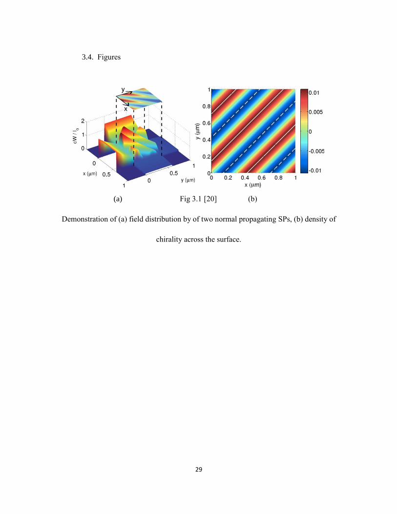
Genet et al. [20] show an effective way to generate chiral optical field. They use two
coherent surface plasmons (SP) propagating perpendicularly with each other on a smooth
metal film to generate a chiral field. This chiral field distribution will induce chiral force
onto chiral particles or molecules. The discussion starts by introducing the density of
chirality and the flow of chirality of an electromagnetic field [21-23]:
𝐾(𝐫, 𝑡) =𝜀
2𝐄 ⋅ (∇ × 𝐄) +
𝜇
2𝐇 ⋅ (∇ × 𝐇),
𝚽(𝐫, 𝑡) =1
2𝐄 × (∇ × 𝐇) −
1
2𝐇 × (∇ × 𝐄). (3.1)
Next, by analyzing one SP mode propagating on a metal-dielectric interface, the paper
gives the electromagnetic field distribution of this evanescent field. By proving the field
generated by SPs can superpose with each other, they give a simulated result of the field
distribution by two normal propagating SPs. As shown in Fig 3.1(a). Then, use (24) to
evaluate the density and flow of chirality on the same interface. Fig 3.1(b) shows 𝐾(𝐫) as
a function of position across the surface, normalized by 𝜔𝑰1,2 𝑐2⁄ . The dashed line and the
solid line represent the minimum and the maximum of the chirality density.
24
In reality it is not easy to reproduce the exact situation illustrated in this paper since the
field by SPs are evanescent. However, the field maximum of CPL are constantly changing
in direction either clockwise or counterclockwise, so the fields generated by CPL should
also have chirality.
3.2. Discriminative force and optical trapping
Many methods have been developed to realize asymmetrical or chiral field distribution,
and using these field many proved that discriminative force exist on enantiomers. Chan
and Wang [15] here brings up a very intriguing result that chiral discriminative force can
happen even with linear polarized light on opposite handedness enantiomers, given the
right condition.
The setup of the experiment is a chiral particle, represented by spring here, on a substrate
experiencing longitudinal incident linearly polarized light. The spring is made of gold and
has an inner radius of 50nm and outer radius of 150nm and pitch P=300nm. As shown in
Fig 3.3 [15], a lateral force in y direction will appear and, according to the handedness of
the spring this force will have opposite direction. The blue arrow shows the handedness of
the spring in the diagram. Notice that the springs in Fig 3.3 (a) and (c) without any substrate
will have only scattering force acting on them.
The different behavior lies in the field scatted by spring onto the substrate and back to the
spring itself. As shown in Fig 3.4 [15] (a) and (b), the magnetic field distribution on the

25
substrate has an asymmetrical pattern alone the propagation direction. In Fig 3.4 (c), the
relationship between chirality and the magnitude of the force was also discussed. The
number of pitches in a spring represent the chirality and as it grows the force will become
larger.
The result here is intriguing but the asymmetrical field here related closely to the substrate.
The substrate is made of gold so there are many free electrons response to the scattered
field from the spring, if the substrate were dielectric material this field distribution would
disappear. The particles used here are relatively large while our target particles are too
small thus the scattered field would be negligible.
Although this setup is not suitable for small particles, it inspired us about how to generate
fields with chirality. Up to this time, we always use chiral light interacts with chiral
structure, the field generated by this setup is definitely chiral but hard to predict. However,
if we simplify the condition using linear light interact with chiral structure or using chiral
light interact with achiral structure, we could still get a chiral field but much easier to
predict.
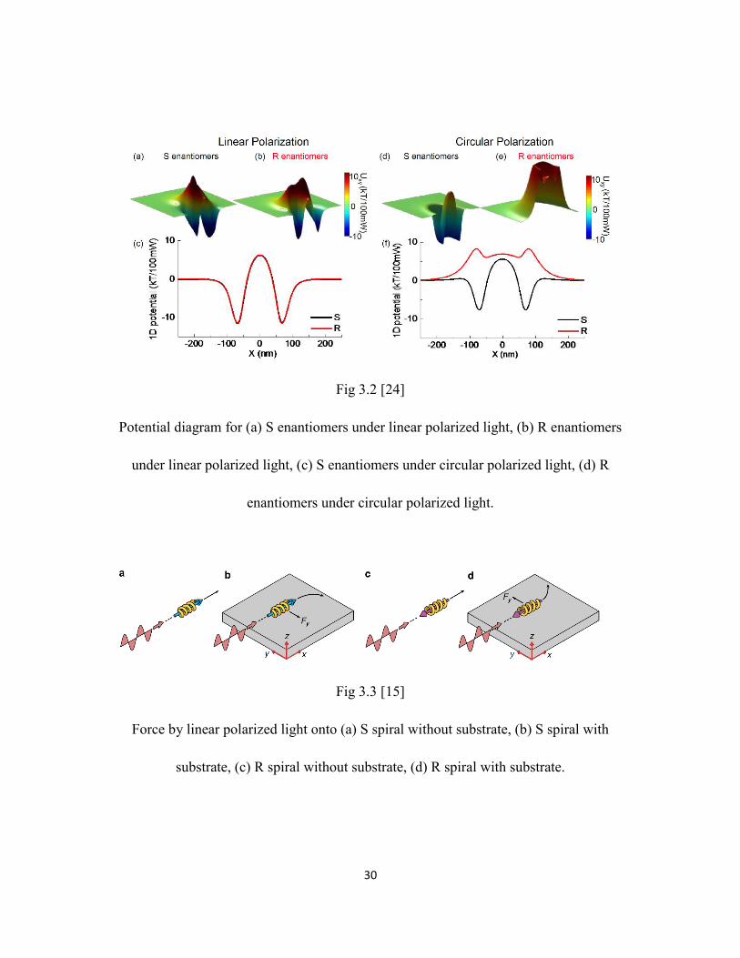
Yang et al. [24] demonstrate a setup of plasmonic optical tweezer powered by CPL which
can selectively trap different handedness nanoparticles. This set up is based on the
interaction between CPL and an achiral structure to generate chiral field distribution. They
start with force calculation with a similar approach as this thesis, then they simplified the
force by several methods. First, they picked out the transverse optical forces (the force

26
acting in the x-y plane). Second, the curl-spin and the vortex force are both small enough
to neglect within the wavelength range they defined. The force is finally reduced to [24]
𝐅𝑡𝑟 =Re(𝛼𝑒𝑒)
4∇|𝐄|2 + Im(𝛼𝑒𝑚)
1
2∇ Im(𝐄 ⋅ 𝐇∗). (3.2)
The nano-aperture has a silver core of radius 60nm and is surrounded by a silicon dioxide
ring of radius 85nm, illuminated by a polarized light with 𝜆 = 711nm. The particles have
a diameter of 10 nm and a chirality 𝜅 = ±2.5.
As shown in Fig 3.2 [24], the S and R enantiomers will experience a similar potential
throughout the cross section of the optical trap if illuminated by linear polarized light.
Whereas the optical trap illuminated by CPL will generate a very different potential curve
upon S and R enantiomers. One of them will experience a flat potential curve so it is
unstable around the trap and the other one will experience a potential well which is perfect
for optical tarping. Since the structure is symmetrical, this difference in trapping force can
only arise from the force discrimination by external fields.
There are several concerns with regards to the result. First, the force calculated in the paper
is relatively small, so we still don’t know whether a stable trapping can be realized under
the influence of Brownian movement. Second, the paper evaluated particles with diameter
of 10nm, the size of a typical organic molecule. This paper assumes they are homogeneous
particles while in reality they are anisotropic. Thus the orientation of the molecule can
change the optical force upon it.

27
3.3. Related experiments
Till now some of the simulations done in related area was introduced, the results from these
works is promising but in reality there are still many difficulties to overcome. The latest
experiment by Hernandez et al. [27] demonstrate discriminative optical trapping using
optical tweezer on chiral particles. The experiment is preformed on isotropic cholesteric
liquid crystal (CLC) particles. The CLC has a unique helix like molecule structure and, by
certain techniques it is made into isotropic small particles. By making them fluorescent,
the behavior of those particles under optical tweezers can be observed. The setup of this
experiment still use a conventional optical tweezer only here a CPL is used. As shown in
Fig 3.7 [27] the particles are attracted under right CPL and repelled under left CPL. Keep
in mind the particles used in this particular experiment is relatively large at around 5μm in
diameter. This size is much larger than molecules but it still shows great potentials.
In above content, we discussed about how linear polarized light interacts with chiral
materials could generate chiral fields. An experiment done by Shimoyama’s group shows
a similar experiment setup and interesting results. In experiment they build a polarization
modulator consists of an array of gold spirals attached on silicon substrate. The spirals are
attached to the substrate at the end and lift off in the middle. By applying air pressure onto
the device, the spirals will be pushed to the side with lower pressure and thus the
handedness of the spirals will change. This can be fine-tuned by adjusting the air pressure
applied. Details of this setup can be found in Fig 3.5 [26].

28
When a linear polarized light (in this paper, with frequency between 0.4-1.8 THz) shine on
the device, it will be modulated as if it went through a wave plate. The maximum azimuth
rotation angle is 𝜃𝑚𝑎𝑥 = 28.7o at 1.0 THz. When the chirality of the spring is different
the rotation angle is also different. Thus by tuning the chirality and the height of the spring
array the rotation angle can be controlled. The paper also talks about the time-averaged
current distribution in the spirals when CPL shine on them. As Fig 3.6 shows, the behaviors
of current distribution are very differently regard to the handedness of the incident light.
These behaviors show the possibility of spiral shaped micro structure manipulate the
incident light field.
In the next chapter we made a similar simulation on spiral structure and incident CPL. The
results show similarity in field distribution. The experiment here does not correspond with
the assumption we made in this thesis. One possible alternative setup of it may be able to
realize chiral field distribution. If a Kretschmann geometry like Fig 1.7 was used and the
evanescent field interact with chiral structure on the interface, a chiral field could be
realized.
29
3.4. Figures
(a) Fig 3.1 [20] (b)
Demonstration of (a) field distribution by of two normal propagating SPs, (b) density of
chirality across the surface.
30
Fig 3.2 [24]
Potential diagram for (a) S enantiomers under linear polarized light, (b) R enantiomers
under linear polarized light, (c) S enantiomers under circular polarized light, (d) R
enantiomers under circular polarized light.
Fig 3.3 [15]
Force by linear polarized light onto (a) S spiral without substrate, (b) S spiral with
substrate, (c) R spiral without substrate, (d) R spiral with substrate.

31
Fig 3.4 [15]
Magnetic field distribution on substrate of (a) S spiral and (b) R spiral. (c) the
relationship between chirality and magnitude of lateral force.
Fig 3.5 [26]
Air pressure controlled chirality MEMS spring.

32
Fig 3.6 [26]
Current density distribution on spiral shined by left and right CPL at (a) 0.45 THz, (b)
0.67 THz, (c) 1.08 THz.
Fig 3.7 [27]
Isotropic small particle made of CLC is attracted by right CPL and repelled by left CPL.

33
CHAPTER 4: EXPERIMENTS AND SIMULATIONS
In addition to the main project, an attempt of making an open source near-field simulation
tool was made. It is called nanoDDSCAT+ and we have done many works. Although the
software is far from perfect, and there are many bugs, but it can now preform calculation
on the electric field, in both vector field and scale field. An option of magnetic field output
is also available, but as discussed below, its accuracy is still in doubt. Further from these
field, with the use of Paraview, the force associate with the particle can be calculated. The
substrate can be single or repeat structure in 1D or 2D. A wavelength swept can also be
done. In this chapter, the basic idea of DDA will be discussed, then the result from
nanoDDSCAT+ will be compared to other software we are using. Followed with a
discussion on data processing and a discussion on chiral optical field generated by spring
structure.
4.1. DDA introduction
DDA, or discrete dipoles approximation, was first developed by DeVoe in 1964 [25] to
calculate the scattering and absorption properties of electromagnetic waves interacting with
arbitrary shapes. The exact solution of Maxwell equations only exists for certain
geometrical shapes like sphere and cylinder, therefore many methods of approaching the
solution was developed. Given enough calculation power, DDA method can approach the

34
exact answer accurately.
The method begins with separate the arbitrary shape large object into discrete dipoles.
Generally speaking, the more dipoles used, the more accurate is the result hence the heavier
the calculation load. Each dipole (i = 1, 2, … , N) is assigned with its own polarizability
𝛼𝑖 and position vector 𝐫𝑖. The polarization of a certain dipole is 𝐩𝑖 = 𝛼𝑖𝐄𝑖 where 𝐄𝑖 is
the superposition of the incident wave and the field contributes by all the other dipoles.
The incident wave 𝐄inc,𝑖 = 𝐄0exp (𝑖𝐤 ⋅ 𝐫𝑖 − 𝑖𝜔𝑡), and 𝐄𝑖 can be expressed as
𝐄𝑖 = 𝐄inc,𝑖 − ∑ 𝐀𝑖𝑘𝐩𝑘𝑘≠𝑖 , (4.1)
where −𝐀𝑖𝑘𝐩𝑘 is the electric field generated by dipole 𝐩𝑘 at 𝐫𝑖 including retardation
effect.
𝐀𝑖𝑘 =exp (𝑖𝑘𝑟𝑖𝑘)
𝑟𝑖𝑘× [𝑘2(�̂�𝑖𝑘�̂�𝑖𝑘 − 𝐈3) +
𝑖𝑘𝑟𝑖𝑘−1
𝑟𝑖𝑘2 (�̂�𝑖𝑘�̂�𝑖𝑘 − 𝐈3)] , 𝑘 ≠ 𝑖, (4.2)
where 𝑘 ≡𝜔
𝑐, 𝑟𝑖𝑘 ≡ |𝐫𝑖 − 𝐫𝑘|, �̂�𝑖𝑘 ≡
(𝐫𝑖−𝐫𝑘)
𝑟𝑖𝑘, and 𝐈3 is a 3×3 identity matrix. Combine all
the equations from i = 1 to N, the electric field at each point can be found.
4.2. nanoDDSCAT+
The nanoDDSCAT+ is based on the free software developed by Draine et al. [17], who also
improved the original DDA method. They applied fast Fourier transformation and
conjugate gradient method to solve convolution problem in large target DDA calculation.
They also published an open source code called DDSCAT which is the core of our software.
Before I joined the group a user interface was developed and by than it can only preform

35
calculation on electric field distribution. The accuracy was satisfying compare to the other
software.
According to equation 3.1 the result of the scattering field is already with their direction
information. Which means adding the vector field to the software is straight forward.
Notice that the result given here are discrete values because of the nature of DDA. So the
first improvement we made to nanoDDSCAT+ was to add a vector field output option.
In the calculation process, all the magnetic permeability of the materials is considered as
𝜇0, same as the permeability of vacuum. Therefore, the magnetic field calculated under this
condition is definitely wrong. However, if the discrete dipoles are also treated as magnetic
dipoles with its corresponding magnetic permeability, and with a similar method derived
above, a magnetic field distribution can also be obtained.
Unfortunately, we didn’t come up with the right code for this part. The attempts to calculate
magnetic field all failed because the results don’t make physical sense. Many our results
break symmetry where is apparently shouldn’t. We still added the option of vector magnetic
field output. Thus, as long as the right code is developed in the future, we can use this
function immediately. Based on the magnetic field data we got, we did some other
calculations to further evaluate the accuracy of the magnetic field. Now with an incident
electromagnetic field on a plasmonic structure, we can get the time averaged electric and
magnetic field (not accurate), both in vector form.

36
4.3. comparison of nanoDDSCAT+ and other software
We now compare the results of simulation on certain structures in two software. The setup
in as following. On a large silicon dioxide substrate, two triangle shape pillar are place tip
to tip like a bowtie. The detailed dimensions are illustrated in Fig 4.1 drew by one of our
team member Qing Ding. The bowtie is made of gold and have a thickness of 50nm. The
simulation used only one bowtie to study its individual behavior. The dimension of the
substrate isn’t too important here as long as it is significant larger than the bowtie. Here we
used 400nm × 400nm × 100nm silicon dioxide substrate.
The results can be found in Fig 4.2 and 4.3. Fig 4.2 shows the resonant peak of absorption
cross section found by two software, and they both are around 700nm. Fig 4.3 (a) and (b)
show the electric field distribution of same setup in Lumerical and nanoDDSCAT+
respectively. The distribution diagrams show great resembling, while the maximum
intensity are different from each other.
4.4. data processing for force calculation
The force on a particle can be calculated using Maxwell stress tensor, by integral the
Maxwell stress tensor around a surface enclose the target particle. The software we use
here is developed by one of our team member Jinlong Zhu. However, the electric and
magnetic field we obtained from nanoDDSCAT+ is the field across the whole space.
Therefore, further data processing is needed. Theoretically, any surface encloses the

37
particle we are trying to analyze can be used, but since in DDA method all the discrete
dipoles are considered as a radiate source, so the choice of the surface must exclude any
other materials in the system.
In this process we used an open source software named Paraview. Since the coordinates of
the points are hard to find, the process to find desired data was a little complicated. First,
cut out a cubic box encloses the particle and extract all the data points inside the box.
Second, inside the box cut another slightly smaller box concentric with the big one and
extract the data points outside it. The remaining data is a 2D cube with electric and
magnetic field information on all sides. According to method of Maxwell stress tensor, the
surface could be chosen arbitrarily, here we chose a small cube close to the particle because
this will dramatically reduce the amount of data we need to process. If we take the whole
space above the substrate, the date points we need to process is around 160000, compare
at 4059 points we got from the small box.
4.5. Spiral structure simulation
Besides the attempt to calculate force associate with small particles, we also did several
interesting simulations on spiral shaped nano-antenna with incident circular polarized light.
This experiment features the same substrate with the bowtie structure, a 4 round spiral with
thickness of 50nm, width between 3nm to 8nm, and gap of 5nm was used here. Two
simulation was performed with same experiment setup and different incident light, one

38
with left CPL and one with right CPL. The results for left and right CPL are shown in Fig
4.4 respectively. We can clearly see the distribution of spots for high electric field density
are different for left and right CPL. This result indicated that the handedness of light does
effect the field distribution when interact with certain structure also with chirality.

39
4.6. Figures
Fig 4.1
Dimension of nano bowtie antenna array.

40
Fig 4.2
The comparison of absorption cross section results between Lumerical and
nanoDDSCAT+.

41
(a) Fig 4.3 (b)
Simulation result on single nano bowtie antenna in (a) nanoDDSCAT+, (b) Lumerical at
𝜆 = 780nm.

42
(a) Fig 4.4 (b)
Field distribution of (a) left CPL, (b) right CPL onto spiral structure at 𝜆 = 780nm.
43
CHAPTER 5: DISCUSSION AND CONCLUSION
In summary, this thesis starts with a calculation of the force on a chiral particle under a
time variant electromagnetic field. It then reviewed some of the latest works followed by
discussion of the results, especially on how to generate chiral fields. This is followed by a
brief introduction of our near-field simulation tool nanoDDSCAT+. Using nanoDDSCAT+
we have done several simulations and the results correspond to what we discussed in
Chapter 3.
There are still some remaining challenges we are facing now. First, the molecules have
irregular shape which means the orientation of molecules will change the optical force they
will experience. One potential solution is to add a strong static external electric field. This
field will apply a torque on all the dipoles so that they will align in the same direction.
Second, the molecules we are trying to manipulate are small and are effected by Brownian
motion, so the optical force must be large enough to overcome this random movement.
Third, the method we discussed in this thesis will be used mostly on organic molecules,
these molecules are usually sensitive to short wavelength light. The photon in the
ultraviolet art of the spectrum has the energy to break down the molecular structure.
Therefore, either we need to isolate molecules from the incident light or we can only use
visible or infrared light. This restriction may bring new challenges. For example, plasmonic
structures usually have at least a single resonant peak wavelength. Therefore, a restriction
on wavelength leads to a restriction on structure dimension.

44
REFERENCES
[1] Circular Dichroism (CD) Spectroscopy,” Circular Dichroism (CD) Spectroscopy |
Applied Photophysics. [Online]. Available:
https://www.photophysics.com/resources/tutorials/circular-dichroism-cd-spectroscopy.
[Accessed: 06-Dec-2016].
[2] Rekoske, James E. "Chiral separations." AIChE Journal 47.1 (2001): 2-5.
[3] Faber, Kurt. Biotransformations in organic chemistry: a textbook. Springer Science &
Business Media, 2011.
[4] Chaumet, Patrick C., and Adel Rahmani. "Electromagnetic force and torque on
magnetic and negative-index scatterers." Optics express 17.4 (2009): 2224-2234.
[5] “Molecules in the mirror - - Enantiomer separation using capillary electrophoresis,” -
Enantiomer separation using capillary electrophoresis. [Online]. Available: http://q-
more.chemeurope.com/q-more-articles/55/molecules-in-the-mirror.html. [Accessed: 06-
Dec-2016].
[6] Jones, Philip, Onofrio Maragó, and Giovanni Volpe. Optical tweezers: Principles and
applications. Cambridge University Press, 2015.
[7] Quidant, Romain, Dmitri Petrov, and Gonçal Badenes. "Radiation forces on a Rayleigh
dielectric sphere in a patterned optical near field." Optics letters 30.9 (2005): 1009-1011.
[8] Quidant, Romain, et al. "Sub-wavelength patterning of the optical near-field." Optics
express 12.2 (2004): 282-287.
[9] Quidant, Romain, Dmitri Petrov, and Gonçal Badenes. "Radiation forces on a Rayleigh
dielectric sphere in a patterned optical near field." Optics letters 30.9 (2005): 1009-1011.
[10] Righini, Maurizio, et al. "Parallel and selective trapping in a patterned plasmonic
landscape." Nature Physics 3.7 (2007): 477-480.
[11] Righini, M., C. Girard, and R. Quidant. "Light-induced manipulation with surface
plasmons." Journal of Optics A: Pure and Applied Optics 10.9 (2008): 093001.

45
[12] Righini, Maurizio, et al. "Surface plasmon optical tweezers: tunable optical
manipulation in the femtonewton range." Physical review letters 100.18 (2008): 186804.
[13] Jackson, John David. Classical electrodynamics. Wiley, 1999.
[14] Stratton, Julius Adams. Electromagnetic theory. John Wiley & Sons, 2007.
[15] Wang, S. B., and C. T. Chan. "Lateral optical force on chiral particles near a surface."
Nature communications 5 (2014).
[16] Aspnes, D. E. "Local-field effects and effective-medium theory: A microscopic
perspective." Am. J. Phys 50.8 (1982).
[17] Draine, Bruce T., and Piotr J. Flatau. "Discrete-dipole approximation for scattering
calculations." JOSA A 11.4 (1994): 1491-1499.
[18] Lakhtakia, Akhlesh. Selected papers on natural optical activity. Vol. 15. Society of
Photo Optical, 1990.
[19] Lindell, Ismo V., et al. "Electromagnetic waves in chiral and bi-isotropic media."
(1994).
[20] Canaguier-Durand, Antoine, and Cyriaque Genet. "Chiral near fields generated from
plasmonic optical lattices." Physical Review A 90.2 (2014): 023842.
[21] Lipkin, Daniel M. "Existence of a new conservation law in electromagnetic theory."
Journal of Mathematical Physics 5.5 (1964): 696-700.
[22] Bliokh, Konstantin Y., and Franco Nori. "Characterizing optical chirality." Physical
Review A 83.2 (2011): 021803.
[23] Cameron, Robert P., Stephen M. Barnett, and Alison M. Yao. "Optical helicity of
interfering waves." Journal of Modern Optics 61.1 (2014): 25-31.
[24] Zhao, Yang, Amr AE Saleh, and Jennifer A. Dionne. "Enantioselective Optical
Trapping of Chiral Nanoparticles with Plasmonic Tweezers." ACS Photonics 3.3 (2016):
304-309.
[25] DeVoe, Howard. "Optical properties of molecular aggregates. I. Classical model of
electronic absorption and refraction." The Journal of chemical physics 41.2 (1964): 393-

46
400.
[26] Kan, Tetsuo, et al. "Enantiomeric switching of chiral metamaterial for terahertz
polarization modulation employing vertically deformable MEMS spirals." Nature
communications 6 (2015).
[27] Hernández, Raúl Josué, et al. "Attractive-repulsive dynamics on light-responsive
chiral microparticles induced by polarized tweezers." Lab on a Chip 13.3 (2013): 459-467.