STUDY OF FIBER MOTION IN MOLDING PROCESSES BY MEANS OF

A MECHANISTIC MODEL

by

Daniel Ramírez

A dissertation submitted in partial fulfillment of the

requirements for the degree of

Doctor of Philosophy

(Mechanical Engineering)

at the

UNIVERSITY OF WISCONSIN-MADISON

2014

Date of final oral examination: 11/13/2014

The dissertation is approved by the following members of the Final Oral Committee:

Tim Andreas Osswald, Professor, Mechanical Engineering

Dan Negrut, Associate Professor, Mechanical Engineering

Robert Rowlands, Professor, Mechanical Engineering

Lih-Sheng Turng, Professor, Mechanical Engineering

Heidi-Lynn Ploeg, Associate Professor, Biomedical Engineering

i

This thesis is dedicated to my parents,

Teresita and Álvaro

ii

ACKNOWLEDGEMENTS

I would like to thank my advisor, Professor Tim Osswald, for his guidance and support.

I would like to thank the faculty serving in my PhD committee: Professor Robert Rowlands,

Professor Heidi Lynn-Ploeg, Professor Dan Negrut, Professor Lih-Sheng (Tom) Turng.

I wish to thank the fellow members of the Polymer Engineering Center for their companionship,

camaraderie, and advice. Specially, I would like to thank Camilo Pérez, Tom Mulholland, Luisa

López, John Puentes, Sebastian Goris, Sean Petzold, and Roberto Monroy. I thank Neil Doll

and Thomas Pfeifer who helped me with the proofreading of this dissertation.

I also thank Jakob Onken, Abrahan Bechara, Sebastian Kollert and Tobias Mattner, for their

contributions to the fiber project.

Finally, I would like to thank my family for their continuous and unconditional support.

iii

CONTENTS

LIST OF FIGURES ....................................................................................................................... v

LIST OF TABLES ......................................................................................................................... x

ABSTRACT ................................................................................................................................. xi

1. INTRODUCTION ............................................................................................................ 1

2. OVERVIEW OF THE LITERATURE .............................................................................. 8

2.1. FIBER ORIENTATION DISTRIBUTION IN TWO DIMENSIONS ................................... 8

2.2. FIBER ORIENTATION IN THREE DIMENSIONS .......................................................... 9

2.3. THE FOLGAR-TUCKER MODEL ................................................................................. 11

2.4. DIRECT SIMULATIONS OF FIBER MOTION IN SUSPENSIONS .............................. 13

MECHANISTIC MODEL SIMULATIONS ..................................................................... 14

2.5. FIBER DAMAGE .......................................................................................................... 20

3. NUMERICAL IMPLEMENTATION .............................................................................. 28

3.1. FIBER BENDING .......................................................................................................... 31

3.2. EXCLUDED VOLUME FORCES .................................................................................. 33

3.3. NEIGHBOR SEARCH ALGORITHM ............................................................................ 35

3.4. PROGRAM STRUCTURE ............................................................................................ 36

iv

4. COMPARISON WITH ANALYTICAL SOLUTIONS AND EXPERIMENTAL WORK

FOR SIMPLE FLOWS ................................................................................................. 39

4.1. NUMERICAL EXPERIMENTS WITH A SINGLE FIBER .............................................. 39

4.2. COMPRESSION MOLDING COMPARISON ............................................................... 43

FIBER MATRIX SEPARATION .................................................................................... 49

FIBER ORIENTATION ................................................................................................. 53

4.3. COMPARISON WITH FOLGAR-TUCKER EXPERIMENTAL RESULTS FOR A

COUETTE DEVICE ...................................................................................................... 56

5. CASE STUDIES FOR COMPLEX FLOWS ................................................................. 60

5.1. FIBER MOTION IN THE FOUNTAIN FLOW REGION ................................................. 60

5.2. STUDY OF FIBER MOTION THROUGH A CONTRACTION ....................................... 68

5.3. DETERMINATION OF THE FOLGAR-TUCKER PARAMETERS FOR NATURAL

FIBER COMPOSITES .................................................................................................. 75

6. CONCLUSIONS AND RECOMMENDATIONS ........................................................... 81

REFERENCES ........................................................................................................................... 84

v

LIST OF FIGURES

Figure 1. Orientation of fibers for different layers in an injection molded disk [7]. ........................ 2

Figure 2. Schematic mold filling [7]. .............................................................................................. 3

Figure 3. Deformation history of a fluid element in the fountain flow region and the

corresponding streamlines in a reference frame that moves with the flow front [13]. ............ 3

Figure 4. Deformation of a polymer particle during injection molding with stretching in the hoop

direction [7]. ........................................................................................................................... 4

Figure 5. Ashing test of a SMC piece [18]. ................................................................................... 5

Figure 6. Fiber content in weight for a compression molded switch box [20]. .............................. 6

Figure 7. Fiber orientation angle ................................................................................................ 8

Figure 8. Fiber orientation distribution function [7]. ....................................................................... 9

Figure 9. Orientation of a single fiber in both spherical and Cartesian coordinate systems [7]. ... 9

Figure 10. Schematic representation of different orientation tensors: (a) unidirectional, aligned

with axis 1, (b) biaxial in plane 1-2, (c) random orientation. ................................................ 11

Figure 11. Mechanistic model simulation developed by Switzer and Klingenberg [37] to study

the formation and dissolution of fiber clusters in a shear flow. ............................................ 17

Figure 12 Illustration of a model of spheres interconnected by springs in order to mimic a

curved particle as proposed by Kittipoomwong and Jabbarzadeh [5]. ................................ 18

Figure 13. Components of the undisturbed flow relative to the fiber which result in: a) bending

moments, b) torsion, c) axial stresses, d) rotation [53]. ....................................................... 21

Figure 14. Fibers subjected to (a) compressive and (b) tensile forces as they rotate in a shear

flow [7]. ................................................................................................................................ 22

vi

Figure 15. Different deformation regimes in a shear flow depending on the fiber stiffness [53]. 23

Figure 16. Fibers being exposed to the hydrodynamic forces as they protrude from pellets which

are being melted in the plasticizing section of an extruder [7]. ............................................ 25

Figure 17. Fiber lengths distribution as a function of rotation speed for a closed twin screw

kneader (Shimizu [60]). ........................................................................................................ 26

Figure 18. Cumulative fiber length distributions of a glass fiber filled polypropylene for different

processing conditions [61]. .................................................................................................. 27

Figure 19. Effects included in the mechanistic model. ................................................................ 28

Figure 20. Discretization of a fiber as a chain of elements and the corresponding balance of

forces and moments. ........................................................................................................... 29

Figure 21. Approximation of a beam by linear segments. ........................................................... 31

Figure 22. Calculation of the normal vector associated to the closest distance between two

approaching cylinders. ......................................................................................................... 34

Figure 23. Example of collision between a fiber and two stationary objects with different friction

coefficients. .......................................................................................................................... 35

Figure 24. Comparison between the orbits calculated using the Jeffrey equations and the orbits

obtained using mechanistic model simulations for a fiber with an aspect ratio rp=10. ........ 40

Figure 25. Orientation distributions for fibers with aspect ratios 10, 15, 20 and 25. ................... 41

Figure 26. Snake orbit which results in fiber breakage. The sequence shows the failure of a fiber

as a result of hydrodynamic forces in a shear flow. ............................................................. 42

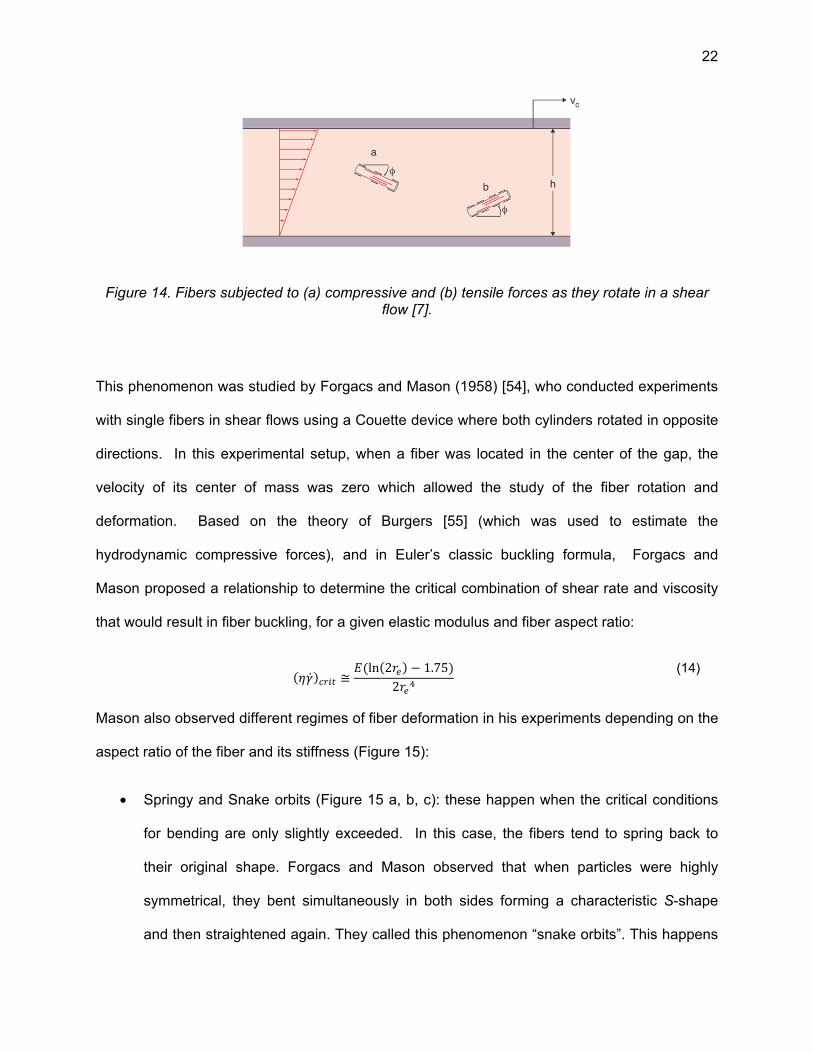
Figure 27. Computer redrawn plot of fibers in a radiograph of a SMC plate which was molded

with an initial mold coverage of 33% [7]. ............................................................................. 44

Figure 28. Measured fiber orientation distribution histogram in a plate with 33% initial mold

coverage [7]. ........................................................................................................................ 44

Figure 29. Influence of the initial charge coverage on the mechanical properties of an SMC plate

[72]. ...................................................................................................................................... 45

vii

Figure 30. Different stages of the compression molding simulation: a) Initial fiber cluster with a

bundle volume fraction of 2.5%, b) Cluster with bundle volume fraction of 25%, c) Final

stage of the simulation, after the fibers have been subjected to a squeezing, planar-

extensional, flow. ................................................................................................................. 48

Figure 31. Fiber separation phenomenon in the simulated SMC part. ....................................... 50

Figure 32. Volume fraction evolution during the compression process for the SMC simulated

plate for the case of an average bundle volume fraction of 25% and no friction between

fibers. ................................................................................................................................... 51

Figure 33. Bundle volume fraction as a function of position for a strain equivalent to 33% mold

coverage, for different simulation settings. .......................................................................... 52

Figure 34. Influence of flow length (obtained via partial filling of the mold) in the relative fiber

content as a function of position for a SMC part. The samples were 2x2 cm2 pieces taken

from SMC plates and are numbered from the flow front position to the initial position of

placement of the charge [79]. .............................................................................................. 52

Figure 35. Fiber orientation comparison with experimental results for strains corresponding to

different initial mold coverages (100, 67, 50 and 33%), no friction between fibers, and a

bundle volume fraction of 35%. ........................................................................................... 54

Figure 36. Comparison between the experimental results and simulation for different bundle

volume fractions and a strain corresponding to 33% mold coverage. ................................. 55

Figure 37. Photograph of Folgar’s experimental set-up with a fiber volume fraction of 16%. Both,

transparent and black tracer polyamide fibers with / of 16 are visible [14]. ..................... 58

Figure 38. Shear cell with periodic boundary conditions used in conjunction with the mechanistic

model to represent Folgar’s experimental set-up with a fiber volume fraction of 16% and a / of 16. ............................................................................................................................. 58

viii

Figure 39. Evolution of the orientation tensor components for the shear cell and their

corresponding averaged orientation distribution histograms for 16% (top), 8% (middle) and

1% volume fraction (bottom). The experimental data was taken from Folgar’s work [14]. .. 59

Figure 40. Schematic representation of the mold filling process in injection molding. ............... 61

Figure 41. Fountain flow streamlines patterns. ........................................................................... 62

Figure 42. Experimental setup for the study of the fountain flow effect [86][87]. ........................ 63

Figure 43. Stream lines of the fountain flow simulation (domain length units in mm). ................ 64

Figure 44. Streamlines and velocity arrow plots for the fountain flow region as calculated by

Mavridis [90] for two reference systems: fixed to the mold walls (left), traveling with the flow

front (right). .......................................................................................................................... 64

Figure 45. Viscosity field for the fountain flow CFD simulation. .................................................. 65

Figure 46. Comparison between the experimental results [87] and the mechanistic model

simulation for piston displacements of 0, 15, 44 and 55 mm. .............................................. 66

Figure 47. Comparison between the experiment [87] and the mechanistic model simulation

(Fountain Flow region detail). .............................................................................................. 66

Figure 48. Fiber orientation as a function of position (fountain flow region) for the mechanistic

model simulation .................................................................................................................. 67

Figure 49. Viscosity curves for the two polypropylenes used in the simulation of the flow through

the gate. ............................................................................................................................... 69

Figure 50. Arrow plot of the velocity field in the flow through a gate of a mold. .......................... 71

Figure 51. Motion of the fiber cluster as it goes through the gate during the simulation. ............ 72

Figure 52. Comparison between the obtained final length distributions (cumulative) for hemp

and ramie fibers in both PP matrices and the initial length distribution. .............................. 73

Figure 53. Fiber orientation distributions in the cluster after going through the gate. ................. 73

Figure 54. Near-gate region including the control volumes at three different time steps. ........... 76

ix

Figure 55. Fiber orientation results comparing the mechanistic model and the Folgar-Tucker

Model. .................................................................................................................................. 79

x

LIST OF TABLES

Table 1. Comparison between dimensionless oscillation periods ( ) for fibers with different

aspect ratios according to Jeffrey and as obtained via the Mechanistic Model simulations.41

Table 2. Dimensions of the periodic boundary cells. .................................................................. 56

Table 3. Properties of the carbon fibers used in the experimental setup used by Onken [87]. ... 63

Table 4. Carreau model parameters. ......................................................................................... 70

Table 5. Natural Fiber Properties ................................................................................................ 70

Table 6. List of simulated natural fiber compounds. ................................................................... 78

Table 7. Predicted fiber interaction coefficients for different natural fiber compounds in matrixes

of polypropylene. ................................................................................................................. 80

xi

ABSTRACT

A mechanistic model was implemented in order to simulate the fiber motion in molding

processes. In this model, each fiber is represented by a chain of segments interconnected by

articulations. A balance of forces and torques is considered in order to determine the velocity

and position of each of these segments during the simulation. This balance includes

hydrodynamic effects (drag forces and torques), fiber-fiber contact forces, and bending

moments.

The model was able to reproduce analytic results such as the Jeffrey [1] orbits for a single fiber

in a shear flow. Also, it was compared with experimental results for SMC (sheet molding

compound process) and for a simple shear flow. In the case of the SMC, the model was able to

reproduce the fiber orientation accurately and the phenomenon of fiber matrix-separation was

captured by the simulations. For the case of a shear flow, the fiber orientation was over-

predicted by the mechanistic model.

The motion of fibers in the fountain flow region and the flow through the gate of a mold were

also considered. In contrast with the research done by other authors (e.g. [2][3][4][5][6]), who

have developed similar mechanistic models to study flows with simple kinematics (for instance

simple shear) to predict bulk properties such as the viscosity of the compound, the work

presented in this dissertation deals with complex flows and uses mechanistic models to study

the phenomenon of fiber attrition and fiber matrix separation.

1

1. INTRODUCTION

Due to their light weight, high specific stiffness and strength properties, and the possibility of

producing parts with complex geometries, molded fiber reinforced plastics have gained

significance and are replacing heavier traditional materials and processes [7][8]. In particular,

they are used in the automotive and aerospace industry where the weight of the parts is of

critical importance. Their use is also increasing in the production of household electronics and

recreational equipment for the aforementioned reasons [9][10].

Mold filling of fiber reinforced resins plays a significant role on part quality in molding processes.

This is reflected in the form of fiber attrition, fiber jamming, and fiber-matrix separation during

manufacturing of fiber filled plastic composite parts. Properties such as strength, stiffness, and

dimensional stability are strongly influenced by the attained fiber orientation, fiber content, and

fiber length, which in turn are determined by the filling process [11][12]. For these reasons, it is

important to develop computational tools to simulate the filling process and study the

phenomena of fiber attrition, flow induced fiber alignment and fiber-matrix separation during

mold filling. The influence of the mold filling process on the fiber orientation in the finished part

can be seen in Figure 1, which shows the fiber orientation in an injection molded disk, where

seven distinct layers can be identified. There are two thin outer layers with a random biaxial

orientation in the disk plane, two thick layers with the main orientation in the flow direction, two

thin randomly oriented layers next to the center core, and a thick layer with circumferential

orientation in the core [7].

2

Figure 1. Orientation of fibers for different layers in an injection molded disk [7].

The surface layer orientation is determined by the Fountain-Flow effect, which occurs in the free

surface of the advancing flow front inside the mold cavity. This effect occurs because of the

non-slip condition in the wall of the mold, which causes a flow from the core of the part to the

wall of the mold as the flow front advances (Figure 2). As soon as the material touches the wall

of the mold, it solidifies and the fiber orientation in the skin of the piece is determined. The name

“Fountain-Flow” arises from the pattern that is observed in the streamlines when a frame of

reference that travels with the flow front is considered. As a result of this effect, there is a

stretching of the fluid elements as they move through the Fountain-Flow region towards the wall,

affecting the fiber orientation. This stretching can be observed in Figure 3, where the

deformation of a rectangular tracer is tracked as it moves through the fountain-flow region. As

the tracer moves towards the wall, it deforms into a characteristic v-shape [13].

3

Figure 2. Schematic mold filling [7].

Figure 3. Deformation history of a fluid element in the fountain flow region and the corresponding streamlines in a reference frame that moves with the flow front [13].

Returning to the analysis of Figure 2, the two thick layers in the disk with orientation in the flow

direction can be attributed to the velocity gradient in the thickness direction. Furthermore, the

orientation in the core of the piece, where the velocity gradient in the thickness direction is equal

to zero, is due to a radial extensional flow, which results in a stretching in the hoop direction and

a fiber orientation which is perpendicular to the flow direction. This flow is shown schematically

in Figure 4, which shows the deformation of a polymer particle as the material flows away from

4

the gate. Now, the thin random layers immediately surrounding the core can be understood as

transitions between the core and the layers with radial orientation.

Figure 4. Deformation of a polymer particle during injection molding with stretching in the hoop direction [7].

In industry, it is common practice to use commercial software for the simulation of molding

processes. These programs allow the prediction of the fiber orientation in molded parts using

fiber orientation models such as the ones proposed by Folgar and Tucker [14](1984), Phelps

and Tucker [15][16] (2009), and Tseng et al. (2012) [17]. All these approaches have their roots

in the original work of Jeffrey [1], who derived the equation of motion for a single ellipsoid

subjected to a shear flow. Therefore, they are intrinsically better suited for the simulation of

compounds with short rigid fibers. However, due to the lack of more accurate models, they are

also used in engineering practice to predict the orientation in long flexible fibers composites. In

many processes such as SMC and LFT (long fiber thermoplastics), fibers are so long they can

bend considerably during molding. For instance, Figure 5 shows an ashing test of an SMC

charge where the polymeric matrix has been burnt in order to observe the glass fibers structure.

5

From the picture, it is apparent that the fibers are considerably bent and deformed. Since fiber

flexibility can be easily taken into account in mechanistic model simulations, they are an

interesting alternative to study fiber behavior during processing.

Figure 5. Ashing test of a SMC piece [18].

Additionally, traditional models for the prediction of fiber orientation include terms to account for

the fiber-fiber interactions which include coefficients that need to be determined experimentally.

Being able to determine the value of these coefficients via simulation (e.g. using mechanistic

models) is desirable because it would reduce costs, and because some compounds are not

amenable to traditional experimental techniques for the determination of fiber orientation. This is

the case for NFC (natural fiber compounds) where typical image analysis methods fail due to

the irregular cross section of the fibers.

Other phenomena in composite processing which are commonly observed but frequently

ignored, and which have important consequences in the design of molded parts, are fiber

jamming and fiber matrix separation. For example, Figure 6 shows the fiber content in different

regions of a molded breaker switch box. Notice that the fiber content in the extreme of the rib is

6

lower than in the rest of the part, which would result in diminished mechanical properties in this

region. For their calculations, engineers rely on mechanical properties that have been obtained

in the laboratory using samples that have simple geometries (without ribs, features or bosses)

and which have been produced under carefully controlled conditions. Therefore, these

laboratory samples present more homogenous fiber contents than the real parts. As a

consequence, the values of the mechanical properties that are being used for designing

complicated parts are frequently overestimated. The phenomenon of fiber-matrix separation has

been studied in this dissertation using a mechanistic model approach following the steps of

Londoño and Osswald [19] .

Figure 6. Fiber content in weight for a compression molded switch box [20].

In the method used in this thesis, fiber motion in compression and injection molding is studied

using a mechanistic approach where fibers are modeled as cylinders with spherical caps

connected by hinges. The model takes into account fiber flexibility, interaction between fibers

and fiber damage. Other authors [2][3][4][5][6] have developed similar models to simulate fiber

motion using mechanistic approaches. However, their work has focused mainly on the study of

simple rheometric flows (simple shear and uniaxial-elongational) in order to predict properties

like the viscosity of the compound and phenomena such as the development of normal stresses

7

and the formation of flocks. Additionally, the work presented in this dissertation deals with

fountain flow and flow through the gate of a mold, which are characterized by more complex

kinematics. The objectives of this work are to use mechanistic model simulations to study the

development of fiber orientation during the molding process and to gain insight into the

phenomena of fiber attrition and fiber matrix separation, which have important consequences in

the quality of molded parts.

This thesis is organized as follows: the second chapter gives an overview of the literature

including the tensorial notation which is used to describe the fiber orientation in molded parts,

the Folgar-Tucker [14] model for the prediction of fiber orientation, and a review of the state of

the art in mechanistic models and fiber attrition. The third chapter presents the fundamentals of

the mechanistic model used in this dissertation and its numerical implementation. It includes a

comparison with the analytical results of Jeffey [1] (which describe the motion of a single fiber in

a shear flow), with experimental results for a shear flow with multiple fibers, and experimental

results for the process of SMC. The fifth chapter deals with the use of the mechanistic model to

simulate flows with more complex kinematics such as the fountain flow, and the flow through a

contraction. The latter is used to study the phenomenon of fiber damage due to the flow through

the gate of a mold. It was found that a possible mechanism for fiber failure is buckling due to

compressive hydrodynamic forces that occur when fibers go from a region of high velocity to a

region of low velocity. This flow is also used to show how mechanistic models can be used to

predict the fiber interaction coefficients. The last chapter includes some general conclusions and

recommendations for future works.

8

2. OVERVIEW OF THE LITERATURE

2.1. FIBER ORIENTATION DISTRIBUTION IN TWO DIMENSIONS

In some molding processes (e.g. sheet molding compound), fibers are so long in comparison

with the thickness of the part, that for all practical purposes, a two dimensional representation of

the fibers is sufficient to define the orientation. In that case, the orientation of a single fiber is

simply given by angle (Figure 7). For a representative volume element (RVE) in a molded

part, the fiber orientation state can be described in terms of a fiber orientation distribution

function ( ), which is defined as the probability that a fiber be oriented between two angles

and (Figure 8. and equation (1)). Since both ends of the fiber are indistinguishable from each

other, the fiber orientation function is periodic: ( ) = ( + ) [7].

( < < ) = ( ) (1)

Figure 7. Fiber orientation angle .

9

Figure 8. Fiber orientation distribution function [7].

2.2. FIBER ORIENTATION IN THREE DIMENSIONS

In three dimensions, the orientation of a single straight fiber is given by a unit vector directed

along the fiber axis or by two angles ( , )in a spherical polar coordinate system, (Figure 9)

[15].

Figure 9. Orientation of a single fiber in both spherical and Cartesian coordinate systems [7].

10

= = cos sinsin sincos (2)

Now, for the characterization of a composite material, it is not sufficient to define the orientation

of a single fiber. Instead the orientation of a fiber population in a representative volume element

needs to be described. In an analogous fashion to the two dimensional case, the fiber

orientation for a collection of fibers is characterized by a probability density function ( )or ( , ), where the probability of a fiber being oriented between and + ,and + is

equal to [15]. A more concise way of describing the fiber orientation is by means

of the second order orientation tensor [15]:

= = ⟨ ⟩ = ⟨cos sin ⟩ ⟨cos sin sin ⟩ ⟨cos sin cos ⟩⟨cos sin sin ⟩ ⟨sin sin ⟩ ⟨sin sin cos ⟩⟨cos sin cos ⟩ ⟨sin sin cos ⟩ ⟨cos ⟩ (3)

Here, brackets signify the average over all fibers in the sample. Alternatively, the tensor can be

defined as the integral (over all directions) of the tensor product weighted by the probability

density function [21]:

= (4)

Although the second order tensor does not contain enough information by itself to completely

reconstruct the original fiber orientation distribution, its succinctness makes it very attractive

from a computational point of view. This is especially the case for the simulation of complex

parts, where keeping track of the fiber orientation distribution in different elements of a mesh

would be impractical. By definition, the orientation tensor is symmetric and its trace is equal to 1.

Figure 10 shows how the fibers in a differential element would look for different orientation

tensor values.

11

Figure 10. Schematic representation of different orientation tensors: (a) unidirectional, aligned with axis 1, (b) biaxial in plane 1-2, (c) random orientation.

2.3. THE FOLGAR-TUCKER MODEL

Fiber orientation effects have a strong influence on the mechanical properties of molded parts.

For this reason, different models for the prediction of the orientation have been developed.

Among these, the most commonly used in commercial software are the Folgar-Tucker model

[14], the ARD model (Anisotropic Rotary Diffusion, Phelps and Tucker [15][16]) and the iARD

model (Improved Anisotropic Rotary Diffusion, Tseng et al. [17]). The first to be developed and

the easier to understand is the Folgar-Tucker model. In order to derive it, the starting point is the

equation of conservation of the fiber orientation distribution [15], which means that one can

relate the amount of fibers that enter and leave a differential volume, carrying a certain degree

of orientation, to the change of the fiber orientation function within the volume. As a result,

equation (5) is developed [16].

= −∇ ∙ ( ) (5)

12

The idea of Folgar and Tucker was to split the right side of the equation into a hydrodynamic

part and a fiber interaction contribution [16] (equation(6)).

= −∇ ∙ + (6)

The fiber interaction term tends to increase the randomness of the fibers in the system, and

from a mathematical point of view it can be described as a diffusion term. The hydrodynamic

contribution corresponds to the motion that a single fiber would describe in a fluid subjected to a

shear flow (Jeffrey orbits) and is given by equation (7):

= ∙ + ( ∙ − : ) (7)

Here, is the vorticity tensor given by = − , is the shear rate tensor given by

= + , is the particle shape parameter given by = , is the particle aspect

ratio, and is the velocity gradient tensor given by = . In order to model the diffusion

term, Folgar and Tucker [14] proposed the relationship:

= − ∇ (8)

Here, is the scalar magnitude of the shear rate tensor , given by = (2 : ) and is the

fiber-fiber interaction coefficient (a fitting parameter). Advani and Tucker [21] used these

equations to formulate a time evolution equation for . This constitutes the standard Folgar-

Tucker model as shown by equations (9) (10) and (11) [16]:

= + (9) = 2 ( − 3 ) (10) = ( ∙ − ∙ ) + ( ∙ + ∙ − 2 : ) (11)

Here, is the fourth order orientation tensor which is defined in an analogous fashion to the

second order one, as seen in equation (12).

13

= (12)

In practice, the fourth order tensor is approximated as a function of the second order one using

a closure approximation [21][22]. For example, a linear closure approximation is given by

equation(13)[22]:

= − 135 + + + 17 + + + + + (13)

where, is the Kronecker delta tensor.

2.4. DIRECT SIMULATIONS OF FIBER MOTION IN SUSPENSIONS

In contrast with the Folgar-Tucker model, where the fiber orientation is considered as a

continuous function, direct fiber simulations are characterized by calculating the motion of each

fiber individually. The behavior of the whole compound can then be studied by averaging the

behavior of all fibers in the simulation.

Direct simulations of fibers in suspensions can be traced back to studies about molecular

modeling in polymer solutions and molecular dynamics. An example of this is the work of Wiest,

Wedgewood and Bird [23], who modeled polymer molecules in a dilute suspension as chains of

beads connected by springs. In a similar fashion, Doi and Chen [24] developed models to study

the kinetics of aggregating colloids in suspensions using a model where particles were

represented as spheres that tended to stick together when they were in contact with each

other. A very influential work in literature is the one of Bossis and Brady [25][26], who introduced

concepts of molecular dynamics into the simulation of particle suspensions using a method

which they called “Stokesian-Dynamics”. This method is based on the solution of the Stokes

equation which governs the motion of Newtonian fluids for low Reynolds number regimes. The

linear nature of the Stokes equation implies that the hydrodynamic force that affects a particle at

14

a given moment is the result of the linear superposition of the forces that result from the

perturbations caused by the motion of the other particles in the system with the hydrodynamic

force that the particle would experience if it were alone in the fluid.

An alternative approach to simulate fiber motion during molding using SPH (smoothed particle

hydrodynamics) has been attempted by Yashiro, Sasaki and Sakaida [27]. This method is

appealing because it automatically couples the equations of motion of the fluid and the fibers.

By doing so, it also includes all the far field interactions with walls and between fibers

themselves. It is a truly meshless method and it is very well suited to represent free surfaces,

such as the one that occurs in the flow front during molding. However, despite of all its

interesting features, SPH does not scale well for polymer processing simulation due to

numerical reasons. Interaction between particles in SPH due to viscous forces is taken along

the line between particle centers. This is not a problem for momentum dominated flows, but

induces numerical errors when dealing with incompressible high viscous flows with low

Reynolds numbers, requiring very small time steps to attain convergence [28].

Similar methods to the ones developed for direct simulations of fiber suspensions have been

used to study a variety of phenomena such as the motion of swimming microorganisms [29][30],

papermaking [31], and DNA decoding [32]. The application of these methods to the simulation

of polymer processes is relatively new with the works of Osswald and Londoño [19].

MECHANISTIC MODEL SIMULATIONS

Other authors have used mechanistic models to study the fiber motion in flows with simple

kinematics such as a simple shear. For instance, in 1993, Yamane et al. [3] developed a model

for the simulation of the motion of rigid rod-like particles for semi-dilute suspensions, including

short distance hydrodynamic interactions and neglecting the long distance ones. They used the

model to predict the Folgar-Tucker interaction coefficients but had poor agreement with

15

experimental results. They attributed the difference to two factors: 1) the experimental

coefficients can vary substantially depending on the technique used to find them, 2) polymer

viscoelasticity was not considered in their model.

In a series of papers (1993-2004), Yamamoto and Matsuoka [33][2][34][35] developed a method

which modeled fibers as chains of bonded spheres. Each pair of bonded spheres could stretch,

bend and twist, allowing the modeling of fiber elongational deformation, bending and torsion

[33]. The motion of fibers was determined from a balance of forces and torques (including

hydrodynamic ones), while neglecting hydrodynamic interactions between spheres. They

studied the behavior of these fibers and demonstrated that the model could reproduce features

such as the characteristic Jeffrey orbits with good agreement regarding both the fiber oscillation

period and in the orbit shape [33]. Also, simulations were performed to determine the intrinsic

viscosity of suspensions of rod shaped particles and its dependence with orientation, rotation

orbit, deformation and fiber aspect ratio[2]. In this method, the sphere chain connectivity was

maintained using constraints which needed to be solved iteratively with the torque and force

balance. Furthermore, in 1995 [34], Yamamoto and Matsuoka extended the method to include

long distance hydrodynamic interactions between the spheres using Stokesian Hydrodynamics.

This approach was used to study the influence of fiber flexibility, concentration, and aspect ratio

on the intrinsic viscosity. Finally, in 2004 [35], they used the model to explore the phenomenon

of fiber fracture in a shear flow.

Most of the work mentioned so far has been for fiber suspensions with relatively low fiber

contents. On the other hand, the work of Sundararajakumar and Koch (1997) [36] focused on

suspensions with higher fiber content and studied the importance of contact forces in

comparison with long distance hydrodynamic effects. Their conclusion was that for dilute and

16

semi dilute suspensions ( << 1)1 the hydrodynamic interactions were dominant. However,

as becomes (1) and suspensions become concentrated, the most relevant mechanism

for increasing the frequency of fiber rotation was the existence of direct fiber-fiber contacts.

They also showed that for sheared rigid fiber suspensions where > 40, neglecting the long

range interactions and including fiber-fiber contacts gives better results in terms of the prediction

of the viscosity, than if the long range interactions are taken into account but the contacts

ignored. The typical fiber concentration in injection molding composites is 2 < < 5, which

corresponds precisely to the range where fiber-fiber contacts begin to be dominant [36] and for

compression molding the typical fiber concentrations are even larger [7]. Since far field

interactions are usually the computational bottleneck of mechanistic models simulations, the

results of Sundararajkumar and Koch, which show that direct fiber contacts dominate the

suspension behavior in the concentrated regime, are of great interest for the potential use of

mechanistic models for the simulation of compounds with realistic fiber contents.

In 1997, Ross and Klingenberg [6], developed a particle-level simulation method to study the

dynamics of flowing suspensions of rigid and flexible fibers; the method is similar to the one

proposed by Yamamoto and Matsuoka, with the main difference that instead of spheres, prolate

spheroids connected through ball and socket joints were used to simulate the fibers. In this

method, hydrodynamic interactions were neglected. The method was used to calculate the

viscosity of fiber suspensions subjected to transient simple shear flow.

Later, Schmid, Switzer and Klingenberg [37][38] extended the model derived by Ross [6] by

modeling the fibers as chains of cylinders with spherical caps. This model, which included

features such as fibers with a non-straight equilibrium shape and fiber-fiber friction, was used to

study the formation of fiber flocks (Figure 11), concluding that these form even in the absence of

1 Here, is the fiber length, is the fiber diameter and is the concentration in terms of fiber number per unit volume.

17

fiber-fiber attraction forces due to an interlocking mechanism which results from the fiber-fiber

friction and the fibers elastic behavior.

Figure 11. Mechanistic model simulation developed by Switzer and Klingenberg [37] to study the formation and dissolution of fiber clusters in a shear flow.

Another model where fibers are modeled as beads connected by springs was developed by

Kittipoomwong and Jabbarzadeh [5]. The model simulated curved particles as beads connected

with hookean springs forming a subunit that is repeated to form the entire fiber (Figure 12). This

kind of model included long range interactions between fibers using the Rotne-Prager-

Yamakawa [39][40] approach. Instead of solving the mobility matrix of the system, they used an

iterative approach where the beads velocity in the previous step was used to estimate the long

range interactions. This model was used to study the effect of fiber shape on the rheology of

fiber suspensions, observing a monotonic increase of the viscosity as the fiber curvature

increases.

18

Figure 12 Illustration of a model of spheres interconnected by springs in order to mimic a curved particle as proposed by Kittipoomwong and Jabbarzadeh [5].

In 2007, Lindström and Uesaka [41] developed a mechanistic model for the study of fiber

suspensions based on the one proposed by Schmid and Klingenberg [37]. There are several

interesting features in this new model including the consideration of fiber inertia and an artificial

damping (viscoelastic term) for the calculation of fiber bending. They found that by including this

artificial damping in the fiber bending moment, the stability of the simulations was greatly

enhanced, allowing the use of much smaller time-steps. The most important innovation in their

work is that they managed to have a two way coupling of the fiber and matrix phase by

enforcing the momentum conservation equation. This was achieved by discretizing the domain

in cells and using a finite difference scheme to solve the Stokes equation, where an additional

body force type term was included for each cell in order to account for the influence of the fiber

motion on the fluid. The model was used to study the rheology of fiber sheared suspensions

[42][43] and the forming of fiber networks during the process of papermaking [31].

Moving forward, Yamanoi and Maia [4][44](2010) presented a model which they designated as

Particle Simulation Method (PSM) to simulate the behavior of concentrate fiber suspensions,

including hydrodynamic interaction between fibers and collision forces. In this model, fibers

were simulated as chains of spheres. The model was used to study the behavior and properties

19

of fiber suspensions (steady state viscosity, intrinsic viscosity, fiber orientation tensors, and

normal stresses) for simple shear. Additionally, the change of the viscosity in extensional flows

was studied [45].

Among other authors who have done research with mechanistic model simulations to study

different phenomena, it is important to mention the work of Saintillan et al. [46][47] who used

mechanistic models based on Slender-Body theory to simulate phenomena such as the

sedimentation fiber suspensions with deformable particles. In the Slender-Body approach [48],

the disturbance due to the movement of a slender body in a fluid is represented by a line

distribution of Stokeslets, which can be defined as singularities due to the application of point

forces. Saintillan studied dilute suspensions with far field hydrodynamic interactions between

particles. In order to simulate an unbounded system, periodic boundary conditions with a

particle-mesh Ewald algorithm, was used. Saintillan also used a similar model to study the

motion of polarizable slender rods subjected to electrophoresis [46][47], focusing on the

hydrodynamic interaction between them and studying the evolution of bulk properties of the

suspensions such as hydrodynamic diffusivities and orientation probabilities, and on the

formation of concentration instabilities. Also, Saintillan used a similar approach to study the

phenomenon of shear-induced migration of polymers in a pressure driven flow. In this approach,

polymer chains are modelled as chains of slender bodies connected by freely rotating joints

[49].

In 2013, Wang et al. [50] [51] developed an approach where fibers were represented by chains

of rigid segments and each of them were modelled as a shell of beads. The hydrodynamic

interactions between these spheres were calculated using the Rotne-Prager-Yamakawa

approach [39][40]. The model was used to study the motion of single curved fibers in a shear

flow. These fibers drifted in the gradient direction of the flow as a result of three different

motions: spinning, “scooping” (the fiber tries to move in a circular pattern given by the fiber

20

curvature), and flipping. Also, the authors showed that the drifting motion was strongly

influenced by the initial fiber orientation.

Other alternative method which couples the equations of motion of the fluid with the ones of the

fibers, using a lattice Boltzmann method, has been proposed by Wu and Aidun [52]. In this

approach a fixed lattice is used to discretize the domain and the fibers are simulated as chains

of segments with spherical hinges that move through the domain. The method was validated

comparing it with results of the literature for viscosity as a function of fiber volume fraction, and

single fiber motion analytical data.

2.5. FIBER DAMAGE

The fiber length distribution (in addition to fiber content, fiber-matrix interaction, and fiber

orientation) is one of the most relevant factors that affect the mechanical properties of a

compound. Typically, longer fibers in a compound result in superior mechanical properties. For

this reason it is important to minimize the fiber breakage that happens during processing. Fiber

breakage occurs due to the hydrodynamic forces that the polymeric matrix exerts on fibers, the

interaction between fibers themselves, and the forces exerted by the moving surfaces of the

machinery used in the process.

The theory about fiber orientation which has been reviewed so far was derived considering rigid

fibers. In order to understand the phenomenon of fiber attrition, it is important to study the

behavior of flexible fibers which deform due to stresses generated by hydrodynamic forces.

Also, in order to gain insight about the stresses generated on fibers in a flow, the components of

the undisturbed field relative to the fiber can be analyzed according to the classification

proposed by Salinas [53] (Figure 13): a) Velocity component perpendicular to the fiber axis,

which can originate bending moments; b) Velocity gradient perpendicular to the fiber axis, which

21

result in torsional torques; c) Velocity along the axis, which causes either tensile or compressive

forces; d) Gradient perpendicular to the axis of axial velocity, which produce a moment that tend

to rotate the fiber and allow the fiber to rotate and cross the streamlines in a shear flow.

Figure 13. Components of the undisturbed flow relative to the fiber which result in: a) bending moments, b) torsion, c) axial stresses, d) rotation [53].

Considering the c) component in the previous classification, when a fiber is in a shear flow and

rotates according to Jeffrey theory, one side of the fiber tends to translate faster than the other

due to the velocity gradient. As a result, it will be alternatively subjected to tensile and

compressive loads as it rotates prescribing the Jeffrey orbit (Figure 14). Although breakage is

unlikely to occur during the part of the cycle when the fiber is in tension, the part of the cycle

when it is in compression can cause shear induced buckling and breakage.

22

Figure 14. Fibers subjected to (a) compressive and (b) tensile forces as they rotate in a shear flow [7].

This phenomenon was studied by Forgacs and Mason (1958) [54], who conducted experiments

with single fibers in shear flows using a Couette device where both cylinders rotated in opposite

directions. In this experimental setup, when a fiber was located in the center of the gap, the

velocity of its center of mass was zero which allowed the study of the fiber rotation and

deformation. Based on the theory of Burgers [55] (which was used to estimate the

hydrodynamic compressive forces), and in Euler’s classic buckling formula, Forgacs and

Mason proposed a relationship to determine the critical combination of shear rate and viscosity

that would result in fiber buckling, for a given elastic modulus and fiber aspect ratio:

( ) ≅ (ln(2 ) − 1.75)2 (14)

Mason also observed different regimes of fiber deformation in his experiments depending on the

aspect ratio of the fiber and its stiffness (Figure 15):

• Springy and Snake orbits (Figure 15 a, b, c): these happen when the critical conditions

for bending are only slightly exceeded. In this case, the fibers tend to spring back to

their original shape. Forgacs and Mason observed that when particles were highly

symmetrical, they bent simultaneously in both sides forming a characteristic S-shape

and then straightened again. They called this phenomenon “snake orbits”. This happens

23

usually when the aspect ratio is approximately 1.5 times the critical aspect ratio [54]. The

transition from the springy to the snake regime can be seen in Figure 15.

• Coiled orbits without entanglement (Figure 15, d): for r>3(rcrit) fibers do not return to their

original shape during rotation.

• Coiled orbits with entanglement (Figure 15, e).

Figure 15. Different deformation regimes in a shear flow depending on the fiber stiffness [53].

Continuing, it is important to discuss some authors which are frequently cited in the literature of

fiber attrition. Turkovich and Erwin [56] studied fiber fracture in reinforced thermoplastic

processing. Their results suggested that in the plasticizing screw, the resulting fiber length

distribution is not significantly affected by the initial length, initial dispersion and fiber fraction.

They found that the theory of fiber breakage for dilute suspensions (Mason) was sufficient to

explain the variation in fiber length during processing. Wall [57] studied fiber attrition during

mixing of polyamide compounds in a twin screw extruder showing that it is the length of the

24

mixing section that affects the length the most, and that as this length was increased, the fiber

length was reduced.

Fisa [58] et al. studied fiber breakage in the compounding of polypropylene with fiber-glass in a

Brabender mixer, finding that the damage was more severe in the initial part of the

compounding process, when fibers were filamentized. Also, they found that the total work

exerted during mixing (found by varying the processing time and the rotor speed) was a good

indicator of the fiber attrition in the system. Contradicting the findings of Turkovich, Fisa found

higher fiber damage (shorter fiber lengths in the compound) for higher volumetric fractions,

implying that fiber-fiber interaction was an important mechanism in fiber attrition. Also, the

viscosity of the melt had an important influence on fiber attrition (higher viscosity resulted in

higher hydrodynamic forces and fiber damage).

Another mechanism for fiber damage exists in the plasticization screw of extruders and injection

molding machines, where the molten plastic coexists with the solid pellets: as the matrix melts,

fibers stick out of the pellets (as if they were cantilevered beams) and they are subjected to

hydrodynamic shear forces and bending moments due to the interaction with the moving fluid,

which generate stresses that can be high enough to cause fiber breakage (Figure 16). This

mechanism was proposed by Gupta [11], who studied the fiber attrition for glass fiber reinforced

polypropylene. Gupta’s experimental setup consisted of an extruder which could be rapidly

cooled in order to extract the screw and gather samples of the different zones, which allowed

the determination of the fiber length distributions in different locations of the screw. The results

of Gupta show that in the case of short fiber composites, most of the fiber damage occurred in

the melting section. In the case of composites with longer fibers, considerable damage occurred

in the compression and post-melting zone.

25

Although some studies [56][11] have shown that most of fiber attrition in the processing occurs

in the screw, the fiber damage in the gate of the mold and in the mold itself is still quite

important [59][7], because that is where the maximum shear rates are attained and is therefore

the limitting factor on the process. Even if the screw had a design that minimizes the fiber

attrition, the high shear rates in the gate of the mold and the mold itself would still cause

considerable fiber breakage, shaping the final fiber length distribution.

Figure 16. Fibers being exposed to the hydrodynamic forces as they protrude from pellets which are being melted in the plasticizing section of an extruder [7].

Shimizu et al. [60] studied fiber damage in a closed twin screw kneader, and the relationship

between fiber length distribution and processing parameters such as barrel temperature, mixing

time, rotation speed (Figure 17), and amount of resin for composites of glass fiber and

polypropylene prepared in an internal mixer. They concluded that the total number of rotations

and shear stress are the major factors which influence the fiber breakage. They also showed

that, in that process, fiber distributions were practically identical if their average length values

were equal.

26

Figure 17. Fiber lengths distribution as a function of rotation speed for a closed twin screw kneader (Shimizu [60]).

In 1996, O’Regan and Akay [59] studied the fiber length distribution in LFT (long fiber

thermoplastics) injection molded parts, finding that it was dependent on the injection molding

nozzle arrangement, geometry of the mold and fiber content.

The recent work by Loken [61] shows how processing conditions influence fiber damage for

injection molding, finding that low processing temperatures and high injection speeds result in

higher fiber damage than high temperatures and low injection speeds. This is in perfect

agreement with equation (14): as temperature decreases the viscosity increases, and with

greater injection speeds, the shear rate also increases. This results in higher stresses and

hydrodynamic forces exerted on the fibers, increasing the likelihood of buckling and damage.

Loken’s results are shown in Figure 18, which shows the cumulative fiber length distribution

for different processing conditions, which is calculated as a function of the fiber length , the

fiber length distribution , and the total length according to equation (15) [7].

(l) = 1 ( ) (15)

27

Regarding the simulation of fiber damage during processing, Phelps recently [62] proposed a

model to predict fiber attrition during the injection molding of LFTs (long fiber thermoplastic

composites). The model is based in basic conservation principles (the total fiber length in the

system should be constant, and if a fiber breaks it generates two fibers whose length should

add to the original one), probabilistic considerations regarding breakage (fibers are more likely

to break in the middle, and therefore a Gaussian distribution for the position of the breaking

point along the fiber is assumed), and Slender-Body theory. A similar model has also been

proposed by Durin [63].

Figure 18. Cumulative fiber length distributions of a glass fiber filled polypropylene for different processing conditions [61].

28

3. NUMERICAL IMPLEMENTATION

In the mechanistic model used in this thesis, each fiber is represented as a chain of segments

interconnected by spherical joints. The model includes effects such as hydrodynamic forces,

fiber flexibility, and excluded volume forces due to fiber-fiber and fiber-walls contacts (Figure

19). Long distance interactions between fibers are neglected due to the high volumetric fractions

found typically in molded pieces [36].

Figure 19. Effects included in the mechanistic model.

In each time step, a force and torque balance (equations (16) and (17)) is performed on each

fiber element obtaining a system of linear equations which yields the velocities and connective

forces in each fiber. These velocities are then integrated over time to determine the fiber

trajectory during the simulation. As with most micro-hydrodynamic models [64], inertial effects

29

are neglected due to the low Reynolds numbers that result from the high viscosity of the

polymeric matrix and the small scale of the fibers.

The hydrodynamic effects are calculated by approximating each segment to a chain of spheres

as shown in Figure 20, and the hydrodynamic force on each bead is given by the Stokes law: = ξ( − ), where ξ = 6 , is the velocity of the fluid evaluated at the coordinates

of the bead , is the velocity of the bead , is the radius of the sphere, and is the

viscosity of the medium. Additionally, due to the fluid’s vorticity, each bead is subjected to a

hydrodynamic torque Tij = ( − ), where = 8 , is the rotational velocity of the

rod, and = × is the macroscopic rotational velocity of the fluid [33]. For the sake of

simplicity all equations were derived for a Newtonian fluid where the viscosity is a constant. In

the non-Newtonian case (which is characterized by the variation in viscosity with the shear rate),

the coefficients and need to be modified to take into account the value of the viscosity

depending on the position of the bead in the flow field.

Figure 20. Discretization of a fiber as a chain of elements and the corresponding balance of forces and moments.

+ − + = 0 (16)

30

− − × + × + [ + × ] = 0 (17)

Here, is a force due to the contact between rods and , and are moments due to

bending, N is the number of rods which are in contact with rod , andN is the number of

beads in rod . Taking into consideration that the velocity of each bead can be decomposed

into the velocity at the hinge and the relative velocity between bead and the hinge, given

by × , these equations can be expanded as:

Additionally, the inextensibility of the chain of rods implies that two rods should have the same

velocity at the point where they are connected, which leads to the following equation:

For each fiber, these equations can be expressed in matrix form as = , where is a

banded matrix, is the vector containing the velocities, angular velocities and the connective

forces of the rods, and contains terms associated with the excluded volume forces, bending

moments (calculated based on the fiber positions for the previous time step) and the ambient

velocity. In order to solve these systems of linear equations, LAPACK and Intel® Math Kernel

Library were used in the project.

− + + ξ( − − × ) = 0 (18)

− − × + × + [β( − ) + ξ × ( − − × )] = 0 (19)

+ × − = 0 (20)

31

3.1. FIBER BENDING

This section presents the approach that is used in the model to calculate the bending moments.

A similar approach was used by Klingenberg [37]. According to the theory of elastic beams [65],

the radius of curvature of an element subjected to bending is given by : 1 = (21)

Where:

: bending moment

: elastic modulus

: inertia moment of a section : radius of curvature of the beam

Additionally, the stress in a beam subjected to bending is equal to:

= (22)

The beam can be approximated by a chain of linear segments (Figure 21) connected by

articulations with hinge springs. The analogy between the two systems is given by equation (26)

which can be deduced using the geometry of the system:

Figure 21. Approximation of a beam by linear segments.

32 = (23) /2 = Sin 2

(24)

For small angles in radians:

Sin 2 ≈ 2 (25)

≈ (26)

Thus, for the simplified system, where the beam is approximated by interconnected rods, the

relationship between the bending moment and the angle is given by:

= (27)

Therefore the bending moment can be calculated as:

= (28)

= ×| × | (29)

Since the fiber deformation is tracked during the simulation, with an appropriate failure criterion,

the model can also predict fiber damage. In order to model fiber attrition phenomena, the critical

failure angle can be defined as:

= (30)

where is the strength of the material. This is of course a very simplified model of fiber

bending and failure, which assumes that fibers themselves behave as an isotropic material.

33

3.2. EXCLUDED VOLUME FORCES

The purpose of the excluded volume forces, which are associated to the contact between fibers,

is to avoid the situation where fibers occupy the same position in space at the same time. Even

if an accurate normal hydrodynamic lubrication between fibers is used, it has been shown

[36][66] that an additional excluded volume force is necessary in order to prevent the fiber-fiber

overlap in mechanistic model simulations. In the model, excluded volume forces increase

gradually as two segments are in close vicinity and approach each other in a collision course.

Some authors have proposed that they be an exponential function of the inverse of the distance

between the surfaces of the fibers [4], or in some cases a function of the type of a Lennard-

Jones potential [19]. In the current version of the program, the force can be calculated by

equation (31), which is similar to the one found in the work of Schmid [37]. In order to determine

the distance, fiber segments geometry is approximated by cylinders with spherical caps. Figure

22 shows how the vector corresponding to the distance between the two pair of segments is

calculated.

= − exp − | | − 2 (31)

Here:

: vector in the normal direction of the two surfaces which can be calculated as =/| | | |: Euclidean norm of vector , which is simply the distance between the two centerlines of

the rods. :fiber radius.

and : excluded volume constants.

34

In the work of Schmid et al. [67] it has been proposed that constant should be a function of

the shear rate, viscosity and segment length. Constants and were determined empirically to

avoid fiber superposition while maintaining reasonable calculation times. This approach is

similar to the one used by Yamamoto et al [34]. In order to determine the distance between the

two cylinders with spherical caps three possible kinds of interactions are considered:

-Spherical cap-Spherical cap

- Cylinder-spherical cap

-Cylinder-Cylinder

For the case of the cylinder-cylinder interaction, which is the more complex one, the vector

can be found with equations (32) and (33) [67]. Also, the case where a spherical cap is in

contact with a cylinder can be easily derived from these equations. In the case when interaction

between spherical caps occurs, the vector is simplyG = − .

= [( − ) ∙ ]( ∙ ) − ( − ) ∙1 − ( ∙ )

= [( − ) ∙ ]( ∙ ) − ( − ) ∙1 − ( ∙ )

(32)

= | + S − − S | (33)

Figure 22. Calculation of the normal vector associated to the closest distance between two approaching cylinders.

35

In addition to the excluded volume force, a friction force which could be included in the balance

of forces can be defined as:

= μ|∆ | ∆ (34)

Here, ∆ is the relative velocity of rod with respect to rod measured at their contact point,

and is the friction coefficient. Preliminary tests in order to assess the implementation of these

forces in the code were conducted for simple cases, such as the collision between a fiber and

two stationary objects having different friction coefficients (Figure 23). In this case, the fiber

slows down more by the side with the higher friction coefficient. In Figure 23, the static fiber on

the left has a higher friction coefficient than the static fiber on the right and thus the velocity of

the moving fiber in the vicinity of the leftmost fiber is lower.

Flow Direction

Figure 23. Example of collision between a fiber and two stationary objects with different friction coefficients.

3.3. NEIGHBOR SEARCH ALGORITHM

In order to determine which fibers are close to each other and about to collide at a given

moment, a list of neighbors is created and updated periodically during the simulation. The naïve

implementation of the neighbor search algorithm would check the distance between all the

rods in the system with each other, which scales with ( ). In order to improve the efficiency

of this search, the domain is divided in cubic cells. All rods in the simulation are classified

36

according to the position that they occupy in this 3D array of cells. Each cell has a unique index

and this index is used as the classification for the rods. Then, it is only necessary to look for

neighbors in the cell where the segment itself is located and in the neighboring ones (a total 27

cells for a cell in the middle of the domain). In order to quickly discard non neighboring rods, a

check based on axis-aligned bounding boxes (AABB) [68] was implemented. These steps

constitute what is called in the literature [68][69] the “broad phase” of the collision detection

algorithm. The second part of the algorithm, known as “narrow phase” uses equations (32) and

(33) in order to precisely determine which segments are interacting with each other.

3.4. PROGRAM STRUCTURE

Although during this research different versions of the program have been developed, the basic

program structure can be represented with the following pseudocode:

call Read_Input_Data

do i=1, number_of_integrations

if (modulo(i, fiber_damage_period)==0) then

call Fiber_Break

call Setup_Grids

call Find_Neighbors

end if

call Fiber_Par_Calc

call Exc_Vol_Forces_Moments

call Bending_Moments

call Fiber_Motion_Solver

call Update_Positions

If (module(i, writ_period)==0) then

Call Data_Out

37

end if

end do

The different program subroutines are these:

Read_Input_Data: this subroutine is the one that reads the input files which contain simulation

parameters such as the fiber diameter, fiber elastic modulus, number of time steps to be

simulated, number of time steps between writing to the output files, critical angle between

segments for breakage, number of time steps between checking for fiber damage and time step

size. Also, the initial segments positions and connectivity are read from files, as well as

information regarding the velocity, vorticity and viscosity field which were obtained using

analytical solutions or numerically using different CFD tools such as OpenFOAM or Comsol in

the case of flows with the complex kinematics.

Break_Fibers: checks if the angle formed by each hinge exceeds the maximum critical angle,

and resets the data structure containing the fiber segments connectivity accordingly.

Set_up_Grids: it sets up the grids for the neighbor list search.

Find_Neighbors: for each fiber segment, this subroutine creates a list of neighboring segments

according to a threshold distance. This search uses an algorithm based on a set of indexed

cells which are used to discretize the domain and speed up the neighbors search.

Fiber_Par_Calc: calls interpolation subroutines to determine the velocity, vorticity and viscosity

fields values for different points located along each fiber segments as required by equations

(18) and (19). It also precalculates geometric properties of the segments to be used by the

subroutine Fiber_Motion_Solver

Exc_Vol_Forces_Moments: calculates the total force which the neighboring segments exert

on each other. It also calculates the total moment generated by these excluded volume forces.

38

Bending_moments: calculates the bending moments according to the angle formed by the

segments for each joint.

Fiber_Motion_Solver: for each fiber, it assembles and solves the matrix that results from the

summation of forces, summation of torques and connectivity constraints (in each fiber joint both

segments must have the same velocity). As a result, the rotational and linear velocities of each

segment, as well as the interconnectivity forces between segments, are obtained.

Update_Positions: updates the fiber segments position using an explicit Euler scheme2.

Data_out: it writes the new segments positions and connectivity information to the output files.

For most of these subroutines (except the ones which involve writing or reading information

from files), and Break_Fibers (which resets the fiber connectivity), the calculations for each

fiber are independent from the other ones. This would allow a relatively easy parallelization of

the code.

The post-processing of the output files is done using different programs which have been written

in Matlab and Fortran. VMD (visual molecular dynamics [70] was used for the visualization of

the fiber motion.

2 In future versions of the program it is advised that a different integration scheme such as Adams-Bashforth be implemented.

39

4. COMPARISON WITH ANALYTICAL SOLUTIONS AND

EXPERIMENTAL WORK FOR SIMPLE FLOWS

4.1. NUMERICAL EXPERIMENTS WITH A SINGLE FIBER

To validate the mechanistic model we can check the two main effects that control fiber

orientation, hydrodynamic effects and fiber-fiber interaction. The acuracy of the hydrodynamic

effect can be tested using the classical analytical approach of Jeffrey [1]. According to this

solution, a fiber subjected to simple shear flow ( = ) rotates in a periodic motion, and its

tip describes an orbit as given by equations (35) to (38) [38].

= + (35)

= ( + 1/ ) + (36)

= 2 + 1 / (37)

= 2 (38)

In Jeffrey’s equations, the position of the fiber is described by angles and , is the orbit

constant (which depends on the initial fiber inclination with respect to the plane of shear), is

the effective aspect ratio, is the period of oscillation, is the fluid shear rate, is a phase

constant and is the rate of spin of the fiber around its main axis. Although Jeffrey’s equations

40

were originally deduced for an ellipsoid, it has been demonstrated that they are also accurate

for cylinders as long as the aspect ratio is corrected using equation(39) [71].

= 1.24ln (39)

Figure 24. Comparison between the orbits calculated using the Jeffrey equations and the orbits obtained using mechanistic model simulations for a fiber with an aspect ratio rp=10.

For a fiber with an aspect ratio of 10, and different initial inclinations, Figure 24 shows a

comparison of the shape of the orbits obtained using the mechanistic model and the Jeffrey

model with good agreement between them.

Also, a comparison was made regarding the orientation probability as shown Figure 25. The

orientation distribution for angle according to the mechanistic model simulation and for the

Jeffrey equation are shown for rigid fibers with aspect ratios 10, 15, 20 and 25. For this set of

simulations fibers were generated in the domain with an initial orientation corresponding to

constant = ∞, which means that they remain in the plane during the whole orbit. Since

fibers are assumed to be rigid in Jeffrey’s theory, the comparison was made with fibers that

were composed by a single rod. As shown by the theory, fibers tend to spend most of the time

-0.8-0.6

-0.4-0.2

00.2

0.40.6

0.8-0.5

0

0.5

0.2

0.4

0.6

0.8

xy

z

JeffreyMechanistic Model

41

oriented in the direction of the flow, with a symmetric probability distribution. The amount of

time that fibers tend to spend aligned with the flow increases for higher aspect ratios. The fit

between the simulation and the Jeffrey model is better for fibers with a greater aspect ratio. For

short fibers, the simulated orientation distributions are broader than the ones predicted by

Jeffrey. There is also a relatively good match regarding the oscillation periods as seen in Table

1. For short fibers, the mechanistic model predicts shorter oscillation periods.

Figure 25. Orientation distributions for fibers with aspect ratios 10, 15, 20 and 25.

rp re Jeffrey Mechanistic

Model

10 8.17 52.11 45.54

15 11.30 71.57 62.99

20 14.33 90.47 89.41

25 17.28 108.93 107.09

30 20.17 127.05 133.66

40 25.82 162.50 177.99

Table 1. Comparison between dimensionless oscillation periods ( ) for fibers with different aspect ratios according to Jeffrey and as obtained via the Mechanistic Model simulations.

−π/2 0 π/20

1

2

3

4

5

6

Pro

babi

lity

Dis

trib

utio

n - ψ

Simulation, rp=10

Simulation, rp=15

Simulation, rp=20

Simulation, rp=25

Jeffrey, rp=10

Jeffrey, rp=15

Jeffrey, rp=20

Jeffrey, rp=25

Orientation Angle - ϕ

42 When a single fiber rotates in a shear flow according to the theory of Jeffrey, it is subjected to

compressive forces due to the fluid’s velocity gradient. As a result, they tend to experience

shear induced buckling. This phenomenon was studied by Forgacs and Mason [54], who

performed experiments in a Couette device with fibers of different materials (Nylon, Rayon and

Dacron) and aspect ratios, and fluids with different viscosities.

Forgacs observed that when particles were highly symmetrical they bent simultaneously in both

sides forming a characteristic S-shapes or Snake orbits and then straightened again. The

characteristic S deformation pattern was also observed during the mechanistic model

simulations (Figure 26).

Figure 26. Snake orbit which results in fiber breakage. The sequence shows the failure of a fiber as a result of hydrodynamic forces in a shear flow.

43

4.2. COMPRESSION MOLDING COMPARISON

In Sheet Molding Compound Process (SMC), a relatively thin charge is put inside a heated mold

and squeezed until the mold fills. Typically, these charges have fiber contents between 20% and

50% by volume, with fiber lengths of around 25 mm, and a thickness between 1 mm and 5 mm

[7]. Since the fibers are so long in comparison with the thickness, their motion is constrained by

the walls of the mold and a planar distribution is sufficient to describe the fiber orientation.

During squeezing, the flow tends to generate fiber orientations with a high degree of anisotropy

which in turn affects the mechanical properties the part. For instance, Figure 27 shows a

computer redrawn plot of the radiography of an SMC plate, where fibers impregnated with lead

have been used as tracers. Although it is very difficult to see a preferential orientation with the

naked eye, an image analysis reveals the fiber orientation histogram in Figure 28.

Figure 29 shows how the mechanical properties change with the anisotropy. For this Figure,

Chen and Tucker [62] compressed charges with initial mold coverages of 33%, 50%, 67% and

100% and the strength was tested in the direction of the flow and in the direction transverse to

the flow. As the percentage of mold coverage decreases, the charge is subjected to greater

strains because it flows longer distances in order to fill the totality of the mold, generating a

higher degree of orientation. As a consequence, the sample with the smallest initial mold

coverage is the one with the highest degree of orientation in the direction of the flow, and

therefore it has the highest strength in the flow direction, but also the poorest one in the

transverse direction.

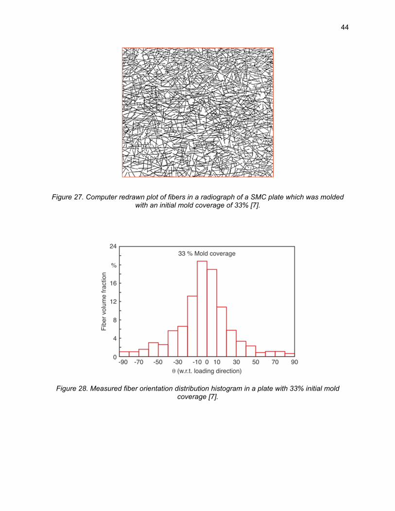
44

Figure 27. Computer redrawn plot of fibers in a radiograph of a SMC plate which was molded with an initial mold coverage of 33% [7].

Figure 28. Measured fiber orientation distribution histogram in a plate with 33% initial mold coverage [7].

45

Figure 29. Influence of the initial charge coverage on the mechanical properties of an SMC plate [72].

As in the previous experimental example about mechanical properties by Jackson, Advani and

Tucker [73], SMC charges were compressed again for 67%, 50% and 33% initial mold

coverage. The fiber fraction was 65% per weight and the final dimensions of the plates were

18in x 12 in x 1/8 in. The orientations were measured by putting tracer fibers with lead and

analyzing radiographies of the plates. In order to measure the initial orientation, Jackson et al.

molded a plate with 100% of the mold coverage and assumed that the orientation of that plate

was representative of the orientation in the charge.

Mechanistic simulations of an SMC process were developed and compared for the experimental

results of Jackson et al. In the mechanistic model, due to computational constraints, instead of

simulating every single fiber, each fiber bundle was simulated as a single chain of segments. At

the beginning of the simulation, these rovings (fiber bundles) were located in a rectangular

46

cluster with a relatively low bundle volume fraction of 2.5%. This bundle volume fraction is

defined as the volume occupied by the bundles divided by the total volume of the charge.

Then, this cluster was “pre-compressed” by means of a mechanistic model simulation using a

velocity field given by equation (39). This velocity field is clearly not a physical one, since it

would violate the mass conservation principle. It is only a computational tool to increase the

fiber concentration in the cluster beyond the point that was feasible with the initial fiber

placement algorithm. At this point, it is important to note that random location of fibers in a

domain, with high volumetric fractions, is not a trivial problem and has been previously studied

by other authors [74][75].

= 0, = 0, = − ℎℎ( ) (39)

After the cluster was “pre-compressed”, the actual simulation of the compression molding

process took place. Let us consider a squeezing flow where the material is restricted by the wall

of the mold in the y direction, is squeezed in the z direction and fills the mold in the x direction.

These restrictions to the fluid motion are similar to the ones found in the compression process of

the charges in Jackson’s experimental setup. A flow that corresponds with this physical situation

is a planar extensional one as given by equation (40), where ℎ( ) is the distance between the

mold walls as they approach each other during the compression molding process. Although this

flow has very simple kinematics and does not consider effects such as the non-slip boundary

condition with the walls of the mold, it has been successfully used to model the compression

molding process [76]. Furthermore, the experimental work of Barone and Caulk [77] shows that

a plug flow, which is similar to the one used here, closely approximates the SMC process.

47

Figure 30 shows three different stages of the simulation: initial fiber cluster, fiber cluster before

being “pre-compressed”, and after being subjected to the squeezing flow.

The diameter of the fiber rovings or fiber bundles is assumed to be 0.5 mm (which is consistent

with the measurements done by Le et al. [78]), with a length of 25 mm and a number of

segments of 16. Additionally, the time-step for the simulation was equal to 1x10-4s, the mold

closing velocity ℎ was set to 1cm/s. The total number of bundles in each simulation was 5099.

In this cluster, bundles are located in planes which are almost parallel to the walls of the mold

that move against each other. An equivalent elastic modulus of 11.7 MPa was considered in

order to calculate the stiffness of the roving. This was calculated assuming that in the roving

each glass fiber has an elastic modulus of 72GPa, that each fiber has a diameter of 15 µm, that

there are 200 fibers per bundle [78], that in bending each fiber takes the same amount of the

moment, and that they can slide freely with each other. This preliminary approach is likely to

underestimate the stiffness of the fiber bundle due to the cohesion between fibers. The matrix

viscosity was assumed to be 100 Pa-s.

The fiber orientation in these planes is chosen to closely resemble the one measured by

Jackson et al. For this purpose, a program was developed to read the experimental histogram

found in Jackson’s paper from a text file.

= ℎℎ( ) , = 0, = − ℎℎ( ) (40)

48

a)

b)

c)

Figure 30. Different stages of the compression molding simulation: a) Initial fiber cluster with a bundle volume fraction of 2.5%, b) Cluster with bundle volume fraction of 25%, c) Final stage of

the simulation, after the fibers have been subjected to a squeezing, planar-extensional, flow.

z

y x

49

FIBER MATRIX SEPARATION

By the end of the simulations, it was clear that the fiber density distribution changed leaving

regions with impoverished fiber content in the borders as shown in Figure 31. This result is

qualitatively consistent with the findings of Schmachtenberg et al. [79] and Kim [80]. This

phenomenon known as fiber-matrix separation, is responsible for weakening regions such as

bosses, ribs [20], and weldlines [79] in fiber reinforced products.

Although at the beginning of the simulation (Figure 32 top) there is a difference in the fiber

content in the borders, due to the fiber placement algorithm, this effect is not sufficient to

generate the difference in fiber content distribution that is observed by the end of the

mechanistic model simulations (Figure 32 bottom). To make this more apparent, two control

tests were performed in addition to the already described simulation: the first test was particle

tracing, where each particle was generated based on the midpoints of the segments from the

mechanistic model simulation and traced using the flow field defined by equation (39); the

second test was a fiber simulation with no fiber-fiber interactions. The results from these tests

are shown in Figure 33.

The particle tracing reveals a difference in the particle volume fraction near the border which

can be attributed to the initial particle placement, and the velocity gradient in the flow direction

(as the velocity will be higher towards the borders of the charge). For the case where no fiber-

fiber interactions were considered, the differences in fiber content at the edges of the charge

were higher than with particle tracing. This can be explained if the non-punctual nature of the

fibers is taken into account, which implies that the flow field has different velocities for different

points in the same fiber. Therefore, the tip of the fiber that is located at the edge of the charge

(where the velocity is highest) will not travel as fast as the surrounding fluid due to the fiber

continuity constraint as other points in the fiber are located in regions where the surrounding

fluid velocity is smaller. With fiber-fiber interactions (especially when friction is included) the

50

results show an even higher fiber-matrix separation than with no interactions. In this case, the

fiber motion is also restricted by other fibers, which tend to form networks and cause a

propagation of these effects. The shape of the obtained curves resembles the experimental

ones obtained by Schmachtenberg [79] as shown in Figure 34 .

Figure 31. Fiber separation phenomenon in the simulated SMC part.

Fiber Rich Region Fiber Impoverished Region

Fiber Impoverished Region

51

Figure 32. Volume fraction evolution during the compression process for the SMC simulated plate for the case of an average bundle volume fraction of 25% and no friction between fibers.

50

0.05

0.1

0.15

0.2

0.25

0.3

0.35

0.4

0.45

0.5

52

Figure 33. Bundle volume fraction as a function of position for a strain equivalent to 33% mold coverage, for different simulation settings.

Figure 34. Influence of flow length (obtained via partial filling of the mold) in the relative fiber content as a function of position for a SMC part. The samples were 2x2 cm2 pieces taken from SMC plates and are numbered from the flow front position to the initial position of placement of

the charge [79].

-0.2 -0.15 -0.1 -0.05 0 0.05 0.1 0.15 0.20

0.05

0.1

0.15

0.2

0.25

0.3

0.35

x [m]

Vol

ume

Fra

ctio

n [-

]

Friction coeff. 0.5

Excl. Volume without Friction

No Excl. Volume

Particle Tracing

53

FIBER ORIENTATION

As with the experiments performed by Jackson, the charges were compressed with strains that

were equivalent to 67% mold coverage, 50% mold coverage and 33% mold coverage.

Regarding the orientation, there is good agreement with the experimental results. For instance

for the highest bundle volume fraction attained in the simulation (35%), the orientation results

are shown in Figure 35. In this figure, 100% represents the initial fiber orientation in the

simulation, which was considered by Jackson et al. as the initial orientation of the charge.

There is a good agreement between the experiments and the mechanistic model simulations.

However, the mechanistic model simulation predicts a higher degree of orientation than the

experiments. This is attributed to the fact that the velocity field in the experiments is more

complex with effects such as the non-slip condition at the wall and the existence of a

component of the velocity which is not necessarily equal to zero. These factors would decrease

the orientation in the direction. Additionally, the fiber matrix separation and the small size of

the simulated clusters cause border effects which result in fibers that do not interact with each

other and are free to align themselves with the flow, without any restriction. Therefore, the

orientation is increased and the histograms are skewed towards a higher degree of alignment.

As a comparison, the results for different volume fractions are presented in Figure 36. Although

the trend is subtle, the fiber alignment decreases for higher volume fractions due to the increase

of fiber-fiber interactions, which is in good agreement with the theory.

54

Figure 35. Fiber orientation comparison with experimental results for strains corresponding to different initial mold coverages (100, 67, 50 and 33%), no friction between fibers, and a bundle

volume fraction of 35%.

−π/2 0 π/20

0.5

1

1.5

Orientation Angle - φ

Orie

ntat

ion

Dis

trib

utio

n - ψ

Mold Coverage 100%

SimulationExperiments

−π/2 0 π/20

0.5

1

1.5

Orientation Angle - φO

rient

atio

n D

istr

ibut

ion

- ψ

Mold Coverage 67%

SimulationExperiments

−π/2 0 π/20

0.5

1

1.5

Orientation Angle - φ

Orie

ntat

ion

Dis

trib

utio

n - ψ

Mold Coverage 50%

SimulationExperiments

−π/2 0 π/20

0.5

1

1.5

Orientation Angle - φ

Orie

ntat

ion

Dis

trib

utio

n - ψ

Mold Coverage 33%

SimulationExperiments

55

Figure 36. Comparison between the experimental results and simulation for different bundle volume fractions and a strain corresponding to 33% mold coverage.

−π/2 0 π/20

0.5

1

1.5

2

Orientation Angle - φ

Dis

trib

utio

n F

un

ctio

n -

ψ

Experiments5%10%25%35%

56

4.3. COMPARISON WITH FOLGAR-TUCKER EXPERIMENTAL

RESULTS FOR A COUETTE DEVICE

The experimental work performed by Folgar in 1983 [14] is compared with the mechanistic

model simulation. For his experiments, Folgar built a Couette device with inner and outer radii of

63.25 and 78.75 mm, respectively (Figure 37). As a fluid, Folgar used a 12500 cS silicone oil.

Folgar randomly placed transparent polyamide fibers (diameter of 0.4 mm) inside the oil with a

few black tracer fibers. The Couette device rotated resulting in a simple shear velocity field with

a shear rate of 0.5 s-1. Folgar took pictures of the fibers in the Couette device and analyzed

them to determine the equilibrium fiber orientation distributions in the system as characterized

by the angle between each fiber and the tangent line to the cylinders in the device.

Folgar’s experiments with 1, 8 and 16% fiber volume fraction, and fibers with an aspect ratio of

16 (6.35 mm long), were reproduced using the mechanistic model. A shear cell (Figure 38) with

periodic boundary conditions was used to emulate Folgar’s experimental set-up. This periodicity

means that as one fiber escapes the domain in the flow direction, it reappears at the other side.

Additionally, one fiber that is about to leave the domain on one side, starts to interact with fibers

on the other side. These periodic boundary conditions apply for the faces of the box with

normals that correpond to the and axis. For the faces, a normal excluded volume force

was used in order to mimick the walls of the inner and outer cylinders. For all volume fractions,

the number of fibers in the cell was set to 754 in order to have the same sample size for the

histograms. The dimensions of the cells used for the three tests are shown in Table 2. The

shear flow velocity field in the domain is given by = [ , 0, 0]. Volume Fraction Lx[m] Ly[m] Lz[m]

1% 0.0620 0.0155 0.0620 8% 0.0219 0.0155 0.0219 16% 0.0155 0.0155 0.0155

Table 2. Dimensions of the periodic boundary cells.

57

For 16% and 8% as the simulation progresses, a quasi steady state of the orientation was

attained (Figure 39). Because of the discrete nature of the mechanistic model, the system can

never reach a perfect steady state condition, leading to fluctuations from time-step to time-step.

This was also the case with Folgar’s experimental measurements. In order to determine the

orientation histograms corresponding to the quasi-steady state, an average of the orientation is

taken between the strain rates denoted in Figure 39 with vertical blue lines.

For 1%, a dampened oscillation is observed in the orientation tensor plots without attaining a

quasi-steady state in the simulation. This oscillation persists without being completely

dampened due to the low collision frequency between fibers, which result from the low fiber

concentration. Since fibers scarcely interact with each other, they move most of the time

according to Jeffrey’s theory. For a fiber with aspect ratio 16, Jeffrey’s equation predicts a strain

of 75.4 for full oscillation period. Since the measured oscillation strain in the plots is equal to

72.0, there is a good agreement with the theory. In the experiment, Folgar observed a

quasisteady state for 1% volume fraction due to the existance of far field interaction forces,

which dominate the process in the dillute regime and which act as dampeners for the oscillation.

Also, if a larger number of fibers were to be used in the simulation, the amplitude of the

oscillations should decrease. For 1% , the average distribution is taken between oscillation

periods as shown in Figure 39.

Since the distributions which are obtained with the mechanistic model are narrower than the

experimental ones, the data suggests that for these relatively low volume fractions, the

mechanistic model underestimates the fiber-fiber interactions. This difference is specially

notorious for the 8% volume fraction simulation, where there is not a good match with the

experimental results. It is suggested that for this intermediate concentration value, far field

58

interactions are probably the ones with more influence in the process, and they are the ones

responsible for the relatively low value of orientation found in Folgar’s experiments. On the other

hand, for the 16% volume fraction case, fibers interact so much with each other via direct

contacts that long range interactions are probably of lesser importance.

Figure 37. Photograph of Folgar’s experimental set-up with a fiber volume fraction of 16%. Both, transparent and black tracer polyamide fibers with / of 16 are visible [14].

Figure 38. Shear cell with periodic boundary conditions used in conjunction with the mechanistic model to represent Folgar’s experimental set-up with a fiber volume fraction of 16% and a / of

16.

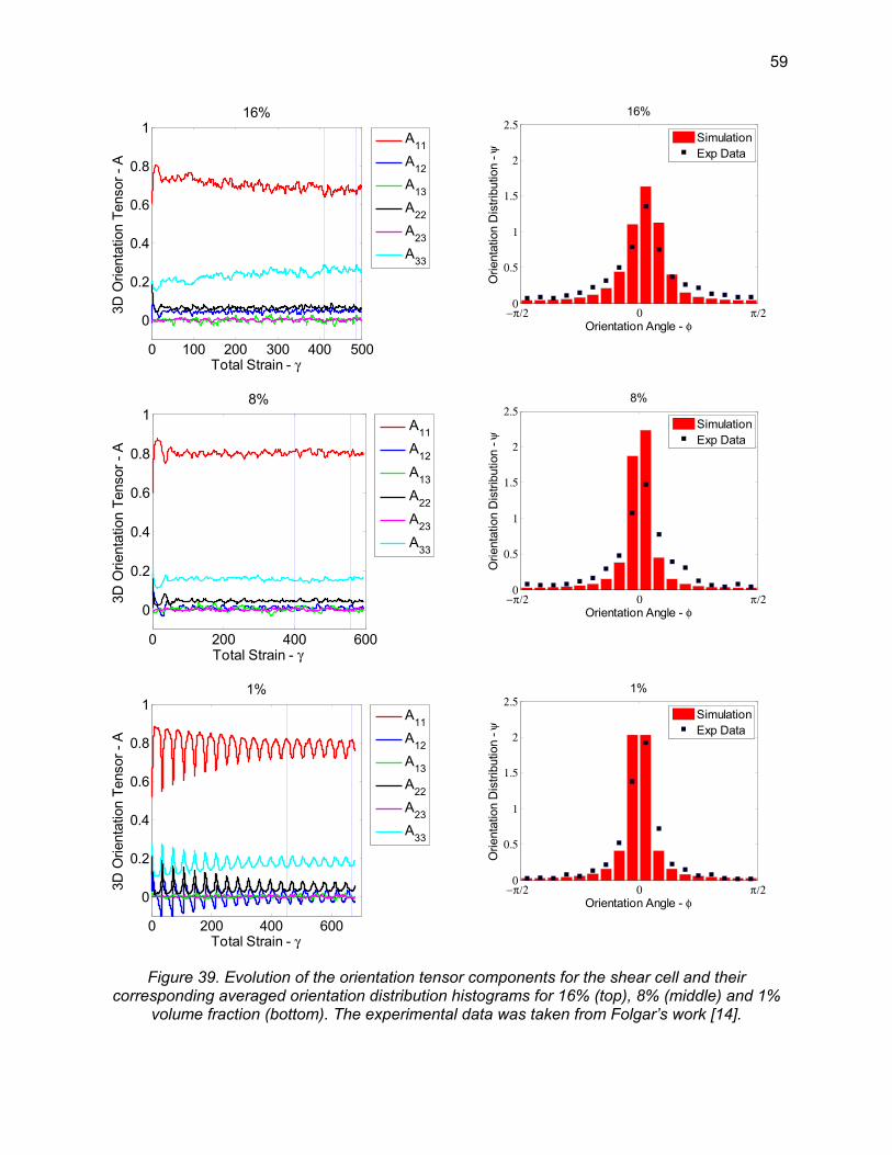
59

Figure 39. Evolution of the orientation tensor components for the shear cell and their corresponding averaged orientation distribution histograms for 16% (top), 8% (middle) and 1%

volume fraction (bottom). The experimental data was taken from Folgar’s work [14].

0 100 200 300 400 500

0

0.2

0.4

0.6

0.8

116%

Total Strain - γ

3D O

rient

atio

n T

enso

r -

A

A11

A12

A13

A22

A23

A33

−π/2 0 π/20

0.5

1

1.5

2

2.5

Orientation Angle - φ

Orie

ntat

ion

Dis

trib

utio

n - ψ

16%

SimulationExp Data

0 200 400 600

0

0.2

0.4

0.6

0.8

18%

Total Strain - γ

3D O

rient

atio

n T

enso

r -

A

A11

A12

A13

A22

A23

A33

−π/2 0 π/20

0.5

1

1.5

2

2.5

Orientation Angle - φ

Orie

ntat

ion

Dis

trib

utio

n - ψ

8%

SimulationExp Data

0 200 400 600

0

0.2

0.4

0.6

0.8

11%

Total Strain - γ

3D O

rient

atio

n T

enso

r -

A

A11

A12

A13

A22

A23

A33

−π/2 0 π/20

0.5

1

1.5

2

2.5

Orientation Angle - φ

Orie

ntat

ion

Dis

trib

utio

n - ψ

1%

SimulationExp Data

60

5. CASE STUDIES FOR COMPLEX FLOWS

This section presents examples of the use of the mechanistic model to study flows with more

complex kinematics. Two cases are considered: the flow in the fountain flow region and the flow

through the gate of a mold.

5.1. FIBER MOTION IN THE FOUNTAIN FLOW REGION

Injection molding is an ideal process for the mass production of parts with complex shapes. It is

one of the most important, common, and economically relevant polymer processes: more than

half of all polymer processing equipment is for injection molding and approximately one third of

all the thermoplastic material manufacturing is done by using injection molding [81]. In the

injection molding process, the material is molten and mixed in the plasticizing unit. Then, it is

injected using high pressure into the mold. When the part has cooled and solidified, it is

removed from the mold. For the sake of study and analysis, the flow inside an injection mold

can be divided into three characteristic regions (Figure 40):

• The gate

• The fully developed region

• The fountain flow

61

Figure 40. Schematic representation of the mold filling process in injection molding.

In the region near the flow front, the material which is traveling in the main direction of the flow

decelerates and spills from the center of the channel to walls. This phenomenon known as the

fountain flow effect (a term coined by Rose [82]) is the only way to fill the regions near the walls

where a non-slip velocity condition exists. As a consequence, all the material that forms the

surface of an injection molded piece has been subjected to a process where it moves through

the centerline of the mold before being deposited on the walls. This has important implications

on the quality of the molded parts, affecting the orientation of the macromolecules and,

therefore, the mechanical and optical properties [83]. In the case of reinforced materials, it

affects the distribution and orientation of fibers [7] [83] [84]. Additionally, the constant flow of

material from center of the mold to the wall necessarily affects the development of the

temperature field during molding. The characteristic streamline patterns of the fountain flow

effect can be seen in Figure 41, where two frames of reference are being used: one is fixed to

the mold (actual streamlines) and the other one travels with the flow front.

62

Figure 41. Fountain flow streamlines patterns.

In this work, the mechanistic model was used to visualize the fiber motion in a fountain flow

region and compared qualitatively with an experimental setup that Kollert [85] and Onken [86]

used for the study of the fountain flow effect. The experimental setup consists of a slit machined

in an aluminum block and a piston (Figure 42). At the beginning of the experiment, three slabs

of polyethylene were placed inside the cavity. The slab in the middle contained carbon fibers.

Then, the sample was melted using electric heating bands and the piston was moved at a

controlled speed resulting in a fountain flow velocity field inside the cavity in the region which is

close to the free surface, where the polymer is in contact with the air. In order to capture

different stages of the fiber motion, several samples where produced with different

displacements. The whole setup was cooled down with water in order to solidify the sample

which was retrieved and observed using an optical microscope.

63

Figure 42. Experimental setup for the study of the fountain flow effect [86][87].

A simulation of the flow in this device was conducted using OpenFoam two phase solver

InterFoam and the Carreau model to take into account the variation of the viscosity with the

shear rate. InterFoam is based on the Volume of Fluid method (VoF). The CFD results were

integrated with the fiber’s mechanistic model allowing the study of fiber motion in the fountain

flow region. The velocity, viscosity and vorticity fields are approximated using a bilinear

interpolation. The properties of the fibers used for the simulation, which are chosen to closely

mimic the experiments, are listed in Table 3. For the initial state of the simulation, the fibers

were scattered randomly within a cluster located at the center of the polymer volume.

Table 3. Properties of the carbon fibers used in the experimental setup used by Onken [87].

Figure 43 shows the stream lines once the model has reached steady state and the fountain

flow effect has completely developed. Two stagnation points can be identified in the cavity

center line: one to the left end on the piston surface, and one to the right on the flow front. The

Property Value

Diameter (µm) 7

Average Length (mm) 0.5

Concentration of the initial cluster (% vol) 5

64

characteristic streamlines patterns in both the polymer and air phase resemble the ones found

by other researchers [88][89]. For instance, Figure 44 shows the streamlines in the classic

paper of Mavridis [90].

Figure 43. Stream lines of the fountain flow simulation (domain length units in mm).

Figure 44. Streamlines and velocity arrow plots for the fountain flow region as calculated by Mavridis [90] for two reference systems: fixed to the mold walls (left), traveling with the flow front

(right).

65

The polymer phase has a variable viscosity field as shown in Figure 45. Carreau’s model

predicts the drop in viscosity when the shear rate is increased. Therefore, the maximum

viscosity occurs in the centerline of the cavity.

Figure 45. Viscosity field for the fountain flow CFD simulation.

Figure 46 and Figure 47show the fiber motion for the experimental setup and the computational

model respectively. As the figures suggest, there is good qualitative agreement between the

experimental results and the simulation. As the fibers approach the flow front, they begin to lag

behind as a result of fiber-fiber interaction. This leads to a fiber-free region at the flow front

which moves towards the surface of the mold, resulting in a fiber-free layer on the outer

surfaces of the part. Figure 48 shows how the orientation of the fibers varies as they move

along the flow front. The color scale represents the magnitude of the fiber’s angle, measured

from a horizontal line located in the center of the cavity. As the fluid decelerates when reaching

the flow front the fibers are jammed together, resulting in significant fiber-fiber interaction; but as

the fibers move away from each other they tend, as expected, to rapidly align with the

streamlines.

66

0 15 44 55

Figure 46. Comparison between the experimental results [87]3 and the mechanistic model

simulation for piston displacements of 0, 15, 44 and 55 mm.

Figure 47. Comparison between the experiment [87] and the mechanistic model simulation (Fountain Flow region detail).

3 In reference [87], the picture aspect ratio was modified in order to better visualize the flow patterns.

67

Figure 48. Fiber orientation as a function of position (fountain flow region) for the mechanistic model simulation

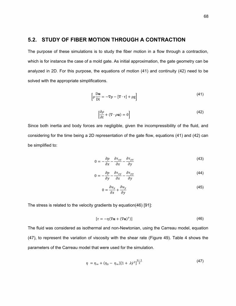
68

5.2. STUDY OF FIBER MOTION THROUGH A CONTRACTION

The purpose of these simulations is to study the fiber motion in a flow through a contraction,

which is for instance the case of a mold gate. As initial approximation, the gate geometry can be

analyzed in 2D. For this purpose, the equations of motion (41) and continuity (42) need to be

solved with the appropriate simplifications.

ρDDt = −∇p − [∇ ∙ τ] + ρg (41)

+ (∇ ∙ ) = 0 (42)

Since both inertia and body forces are negligible, given the incompressibility of the fluid, and

considering for the time being a 2D representation of the gate flow, equations (41) and (42) can

be simplified to:

0 = − − − (43)

0 = − − − (44)

0 = + (45)

The stress is related to the velocity gradients by equation(46) [91]:

[ = − (∇ + (∇ ) )] (46)

The fluid was considered as isothermal and non-Newtonian, using the Carreau model, equation

(47), to represent the variation of viscosity with the shear rate (Figure 49). Table 4 shows the

parameters of the Carreau model that were used for the simulation.

= + ( − )[1 + ] (47)

69

Figure 49. Viscosity curves for the two polypropylenes used in the simulation of the flow through the gate.

The velocity field was then determined with a simulation by Finite Elements using COMSOL.

These results were used as input for with the mechanistic model program. An algorithm based

on radial basis functions [92] and bilinear interpolation was used to interpolate the velocity,

vorticity, and viscosity fields. Before the first time step, the values of these variables were

interpolated for points in a rectangular grid using the data obtained from Comsol and a radial

basis function interpolation scheme [92]. For the rest of the simulation the bilinear interpolation

was used. The advantage of using the latter is that a point can be located within the grid with

very little computational effort. This is important because these interpolations are used every

single time-step and, therefore, they need to be performed as efficiently as possible.

In order to simulate the possible contact with the walls, two types of possible collisions are

considered: the contact between a fiber and a border (where the border can be mimicked as an

infinitely long fiber with a small diameter) and a collision between a plane of the wall and the

1

10

100

1000

1 10 100 1000 10000 100000

η [Pa-s]

γ [1/s]

Moplen 3307,Carreau

Moplen 500,Carreau

Moplen 3307,Rheometric Data

Moplen 500,Rheometric Data

70

fiber. For the latter, it is only necessary to check the contact between the spherical caps and the

walls.

Two kinds of polypropylene were considered as matrixes and natural fibers (ramie and hemp)

as the reinforcers. The properties of the fibers can be found in Table 5. The boundary conditions

for the simulation were as follows:

• Inlet: known average velocity (0.39 m/s)

• Outlet: known pressure ( = 0)

• Walls: no slip boundary condition ( = 0)

Matrix η0 (Pa-s) η∞ (Pa-s) λ (s) n Moplen 3307 1.7×103 0 0.40 0.41 Moplen 500 1.36×103 0 0.40 0.41

Table 4. Carreau model parameters.

Hemp Ramie Average Diameter (mm) 0.0376 0.0198 Ultimate Strength (N/mm2) 827 1250 E- Modulus (N/mm2) 12984 35958

Table 5. Natural Fiber Properties

71

Figure 50. Arrow plot of the velocity field in the flow through a gate of a mold.

The calculated velocity (Figure 50), vorticity and viscosity fields were then used as input data for

the mechanistic fiber model. Figure 51 shows the movement of the fiber cluster through the gate

and the fact that fibers tend to align themselves with the streamlines as flow converges. Also,

the same fibers tend to orient perpendicularly to the streamlines in the diverging flow.

An important aspect to consider when processing composites by molding is the phenomenon of

fiber attrition. This is especially the case for injection molding because this process is

characterized by the development high shear stresses. Although most of the damage is done in

the plasticizing screw, the fiber breakage inside the mold cavity and in the gate region is also of

importance because that is where the highest shear stresses happen in the process [7].

Therefore, since the current understanding of fiber attrition suggests that these stresses are the

ones that tend to break the fibers, the flow through the gate is the one that limits the attained

length distribution.

72

After going through the contraction, the cumulative fiber distributions in the cluster are shown in

Figure 52. Natural fibers break during the simulation resulting in a shift of fiber

percentage from higher lengths to shorter lengths as the fiber cluster moves through the

contraction. This can be explained as a result of the deceleration of the fluid as it leaves the

gate, which generates a velocity difference between each of the fiber’s endpoints. Hence, the

fibers experience buckling, leading to damage and break-up. Ramie fibers are more slender and

break with greater ease, which results in overall smaller fiber lengths than the ones

obtained with hemp. Higher fiber damage is observed for Moplen 3307, which has a higher

viscosity. This is expected because the fiber bending and failure increases with the viscous

forces.

Figure 51. Motion of the fiber cluster as it goes through the gate during the simulation.

73

Figure 52. Comparison between the obtained final length distributions (cumulative) for hemp and ramie fibers in both PP matrices and the initial length distribution.

a) Hemp fibers in Moplen 3307 b) Ramie Fibers in Moplen 3307

c) Hemp fibers in Moplen 50 d) Ramie fibers in Moplen 500

Figure 53. Fiber orientation distributions in the cluster after going through the gate.

Orientation Angle [degrees] Orientation Angle [degrees]

Orientation Angle [degrees] Orientation Angle [degrees]

74

The fiber orientation was also analyzed as shown in Figure 53, where fiber orientations by the

end of the simulation are plotted. At the beginning of the simulation all fibers are horizontal with

an inclination of 0 degrees. Ramie fibers have a higher aspect ratio and therefore they are less

likely to rotate in the flow. This explains the fact that they tend to remain oriented at zero

degrees with less dispersion in the fiber orientation distribution histograms.

75

5.3. DETERMINATION OF THE FOLGAR-TUCKER PARAMETERS

FOR NATURAL FIBER COMPOSITES

This section shows how the mechanistic model can be used to approximate the fiber interaction

coefficients. In this case, the simulations were conducted for different natural fiber compounds.

Natural fiber composites (NFCs) importance in the automotive industry has grown during recent

years. The reasons for this growth have to do with in their environmental friendliness,

renewability, good sound isolating properties and the increased full efficiency due to reduced

weight [93][94][95] .

During processing of fiber reinforced plastic parts, anisotropy is introduced due to fiber

alignment caused by the deformation of the flowing polymer melt. Different models are available

to calculate the development of fiber orientation during processing. These orientation models

include material dependent parameters, which are obtained using experimental techniques

which involve measuring the fiber orientation within the finished parts, and fitting the material

dependent parameters until the model’s fiber orientation distributions match the actual fiber

orientation. For glass fibers, the models and the parameters have been well investigated.

However, data for modeling the orientation distribution development during processing for

natural fiber filled resins is basically non-existent. Furthermore, actual measurements of fiber

orientation distributions within natural fiber filled composites are challenging to obtain.

In this study case, an alternative method has been developed to find the fiber-fiber interaction

coefficient from the Folgar-Tucker model, by coupling both the Folgar-Tucker and the

Mechanistic Model. In this technique, is iteratively optimized until the fiber orientation

distribution computed using the Folgar-Tucker model fits the fiber orientation fields predicted by

the mechanistic model. With this virtual method, the costly measurement of actual fiber

orientation fields within a finished part, and the subsequent re-engineering approach can be

76

avoided. Furthermore, the mechanistic model can be used to determine any material dependent

parameters needed for other fiber orientation predictive models, such as the recently developed

Phelps-Tucker[16] rotational diffusion model.

Figure 54. Near-gate region including the control volumes at three different time steps.

A procedure to determine the interaction coefficients in this flow field using the mechanistic

model is proposed. First, the fiber motion is calculated for a fiber cluster using the mechanistic

model. Three volumes in the domain, where the fiber cluster has gone through are selected as

shown in Figure 54. The trajectory of the fluid particles associated to the center of these

volumes is calculated and the initial position of these three particles is determined. These

particles of fluid are then followed during the simulation and the value of the orientation tensor

around them is determined using the mechanistic model.

77

An initial is then picked for the Folgar-Tucker simulation and a preliminary simulation is

performed (the spatial derivatives of the orientation tensor which are required for the Folgar-

Tucker equations are estimated using a centered finite differences scheme and data from the

mechanistic model. Using a gradient method, the next is chosen and the next simulation with

the Folgar-Tucker model is done. This procedure is repeated until the difference between the

components of the orientation tensors calculated with both models is minimized for the three

control volumes, fulfilling the optimization exit condition5. Thus, the error of the fiber orientation

results for both models is minimized, eventually leading to an optimal . In order to approximate

the fourth order tensor in the Folgar-Tucker equation, a quadratic closure approximation

( = ) was used.

The for different natural fiber compounds were found for the different fiber volume fractions,

fiber lengths, fiber diameters and mechanical properties of the compounds used within this

project (Table 6). The properties shown in this table were measured by K. Albrecht and J.

Müssig [95], from the Hochschule Bremen. Compounds denoted with * have not been

manufactured yet, however, they have been simulated. Two different polypropylene matrices

were used: PP1 (MFI 15) and PP2 (MFI 100). As of now, five different types of natural fibers

were examined: Regenerated Cellulose (CH), Sisal, Hemp, Flax and Kenaf. The fiber volume

fraction was varied within the compounds from 10% to 30% and the fiber / ratio ranges from

9.8 (Sisal) to 33.4 (CH).

5 The program to predict the was developed in collaboration with Philip Schmidtke of M-BaseEngineering & Software GmbH. The author acknowledges that MBase contributed in developing code to iterate the and choose the optimal value, and that they conducted numerical experiments for the different compounds in Table 7. The author contributed by developing the mechanistic model code, the code to find the orientation in the control volumes, and the code to determine the orientation in these control volumes using the Folgar-Tucker model.

78

Fiber Length Diameter MatrixVolume Fraction

E-Modulus Ultimate Strength

[mm] [mm] [MPa] [MPa]

CH 0.401 0.012 PP1 10% 16400 740

CH 0.376 0.012 PP2 10% 16400 740

Flax 0.438 0.02137 PP1 30% 9765 631

Hemp 0.503 0.02725 PP1 30% 22184 953

Kenaf 0.415 0.02565 PP1 30% 15411 1043

Sisal 0.666 0.06766 PP1 30% 20852 1048

Sisal* 0.666 0.06766 PP1 24% 20852 1048

Sisal* 0.666 0.06766 PP1 16% 20852 1048

Sisal* 0.666 0.06766 PP1 10% 20852 1048

Table 6. List of simulated natural fiber compounds.

Figure 55 shows the evolution of the orientation tensor components as a function of position

calculated with the Folgar-Tucker model for a small volume that moves through the domain

(blue solid line). Additionally, the figures show the results for the mechanistic model (red

diamonds) within the three defined control volumes. The results are based on the simulation for

PP1 with 30% Sisal Fibers and a of 0.0055 for the Folgar-Tucker model.

The interaction coefficients as obtained by this method can be found in Table 7. Comparing the

Sisal 2 data, it can be seen that the interaction coefficients are smaller for lower fiber content,

which is the expected trend. The compound with the higher interaction coefficient in this study

was the one with Sisal 2 fibers in a PP1 matrix. This was expected because it corresponds to

the highest fraction (30%). On the other end of the spectrum, the compound with the lowest

interaction coefficient was CH1L1 in PP2, which corresponds to the lowest fiber fraction (10%).

The obtained fiber interaction coefficients are relatively low when compared with compounds

filled with glass fiber, which in general range between 0.01 and 0.04 [96]. Due to the fact that

79

glass fibers are longer and slender, this difference of the comparing natural fibers and glass

fibers is reasonable.

Figure 55. Fiber orientation results comparing the mechanistic model and the Folgar-Tucker Model.

80

Fiber Matrix CI Sisal 2 (30%) PP1 0.0055

Sisal 2 (24%) PP1 0.0049

Sisal 2 (16%) PP1 0.0048

Sisal 2 (10%) PP1 0.0045

Kenaf 1 PP1 0.0039

Hemp 2 PP1 0.0037

Flax 1 PP1 0.0035

CH1 L1 PP1 0.003

CH1 L1 PP2 0.0032

Table 7. Predicted fiber interaction coefficients for different natural fiber compounds in matrixes of polypropylene.

81

6. CONCLUSIONS AND RECOMMENDATIONS

A mechanistic model has been developed to simulate the fiber motion in molding processes.

The model considers hydrodynamic forces, fiber-fiber contact and friction forces, fiber bending,

and fiber damage. The results of the simulations were compared with theoretical results such as

the Jeffrey orbits and with experiments in an extensional planar squeezing flow (compression

molding), fountain flow and shear flow. The phenomenon of fiber breakage when fibers go

through a contraction (e.g. the gate of a mold) was studied, concluding that a possible

mechanism for fiber failure is the buckling that fibers experience due to compressive forces that

arise when they go from a region of high velocity to a region of low velocity. Additionally a

methodology to determine the fiber interaction coefficients (Folgar-Tucker model) using a

mechanistic approach has been proposed.

Regarding future work, long range hydrodynamic forces may be included in the model. Although

the literature [36][66] suggests that for the typical concentrations found in molding processes the

fiber interactions that dominate are short ranged and are mainly due to fiber-fiber contacts and

hydrodynamic lubrication, it is possible that these far field interactions need to be included in the

model in order to have more accurate predictions of the fiber orientations. Specifically, the

consideration of far field interactions in the model may help to improve the accuracy for the

prediction of parameters such as the fiber-fiber interaction coefficient in the Folgar-Tucker

model. These far field effects do not arise only because of the interaction between fibers, but

because of the interaction with the walls of the mold. Far field interactions are notorious for

being the most computationally expensive part of molecular dynamic simulations and

simulations of suspensions, with computational costs that scale with (N ), (N ) or (NlogN) [25][97], depending on the approach. Therefore, if they are to be included in the

82

model it will probably only be for simplified cases such as cells subjected to shear flow with

periodic boundary conditions.

Future codes could aim to couple the fluid equations of motion with the fiber motion along the

lines of the work developed by Lindström [31]. By doing so, the far field interactions between

different fibers would be indirectly taken into account. Also, it would allow for a more accurate

representation of the fluid motion which is an important thing to consider in situations such as

the study of the fiber matrix separation that occurs in the ribs and features of molded parts.

Although these phenomena were studied in this thesis without considering the two-way coupling

of the two phases, this approach is somewhat incomplete because in the phenomenon of fiber

matrix separation, fibers exert a force that delays the motion of the matrix. Ultimately, this

delaying force should be taken into account.

Also, in order to be able to simulate greater fiber quantities, it is important to continue improving

the efficiency of the algorithms. In this dissertation, a preliminary version of the program which

used OpenMP was developed. However, the simulations were done mainly in a single-thread

version of the program. The work on the parallelization of the code needs to be continued using

tools such as CUDA in order to simulate a greater number of fibers in a reasonable amount of

time. This is of the utmost importance if this model intends to be used for the simulation of more

realistic injection and compression molded pieces.

In this thesis, most of the simulations were done for natural fibers, rovings and nylon fibers,

which are relatively thick. The code optimization and parallelization are also critical for the

simulation of thin fibers with extremely high aspect rations (e.g. continuous glass fibers).

Although some attempts have been made in this regard, it has been challenging because it is

necessary to use a large amount of segments in order to be able to attain realistic shapes when

fibers are deformed in bending. Additionally, since glass fibers have such a small diameter

83

(compared for instance with some of the natural fibers simulated in this project), a large quantity

of segments needs to be included in order to even simulate small injection molded pieces,

increasing the computational costs of the simulations.

The equilibrium shape of the fibers in this thesis was assumed to be a straight line. Also, the

torque due to torsion was not considered. Including fibers with different equilibrium shapes and

torsion can be of interest because these features are relevant in the phenomenon of fiber-fiber

interlocking which plays a role in fiber-matrix separation.

A mechanism for fiber damage in the gate of a mold has been proposed with basis on the

simulations made via mechanistic model simulations. However, as have been reported in the

literature, most of the fiber damage occurs in the screw of the injection molding machine. It is

the opinion of the author that the mechanistic model method developed in this dissertation could

be extended to study the fiber attrition in the melting zone of the screw with minor modifications.

In order to do this, a model like the one proposed by Tadmor [84] would be used to describe the

melting rate in the screw.

The algorithms for fiber placement at the beginning of the simulation need to be improved too. It

was observed that the ones developed for this dissertation tend to generate effects which can

be undesirable, such as local fiber alignment with the borders and low obtained volume

fractions. Also, in real processes fibers are not really randomly arranged. Instead, the fiber

arrangement is determined by the physics of the process. For instance, in LFT, fibers tend to

form specific circular patterns given by the extrusion process that is used to produce the

charges. Also, fibers tend to be locally aligned in bundles. Another example is the SMC process,

where fibers are cut during the charge preparation and as a result, they are shorter for regions

near the borders. All these factors need to be considered to make the simulations more

realistic.

84

REFERENCES

[1] G. B. Jeffery, “The Motion of Ellipsoidal Particles Immersed in a Viscous Fluid,” Proc. R. Soc. Lond. A, vol. 102, no. 715, pp. 161–179, Nov. 1922.

[2] S. Yamamoto and T. Matsuoka, “Viscosity of dilute suspensions of rodlike particles: A numerical simulation method,” The Journal of Chemical Physics, vol. 100, no. 4, p. 3317, 1994.

[3] Y. Yamane, Y. Kaneda, and M. Dio, “Numerical simulation of semi-dilute suspensions of rodlike particles in shear flow,” Journal of Non-Newtonian Fluid Mechanics, vol. 54, pp. 405–421, Aug. 1994.

[4] Mikio Yamanoi and João M. Maia, “Analysis of rheological properties of fiber suspensions in a Newtonian fluid by direct fiber simulation. Part 3: Behavior in uniaxial extensional flows,” Journal of Non-Newtonian Fluid Mechanics, vol. 165, no. 23–24, pp. 1682–1687, Dec. 2010.

[5] P. Kittipoomwong and A. Jabbarzadeh, “Effect of fibre curvature on the rheology of particulate suspensions,” Journal of Non-Newtonian Fluid Mechanics, vol. 166, no. 23–24, pp. 1347–1355, Dec. 2011.

[6] R. F. Ross and D. J. Klingenberg, “Dynamic simulation of flexible fibers composed of linked rigid bodies,” The Journal of Chemical Physics, vol. 106, no. 7, p. 2949, 1997.

[7] T. A. Osswald and G. Menges, Material science of polymers for engineers. Munich [Germany]: Hanser Publishers, 2012.

[8] S. K. De and White, Short fibre-polymer composites. Cambridge, England: Woodhead Pub., 1996.

[9] A. B. Strong, High performance and engineering thermoplastic composites. Lancaster, Pa: Technomic Pub. Co, 1993.

[10] M. J. Owen, V. Middleton, and I. A. Jones, Eds., Integrated design and manufacture using fibre-reinforced polymeric composites. Boca Raton, FL: CRC Press, 2000.

[11] M. Gupta and K. K. Wang, “Fiber orientation and mechanical properties of short-fiber-reinforced injection-molded composites: Simulated and experimental results,” Polymer Composites, vol. 14, no. 5, pp. 367–382, Oct. 1993.

[12] S.-Y. Fu and B. Lauke, “Effects of fiber length and fiber orientation distributions on the tensile strength of short-fiber-reinforced polymers,” Composites Science and Technology, vol. 56, no. 10, pp. 1179–1190, 1996.

[13] H. Mavridis, “The Effect of Fountain Flow on Molecular Orientation in Injection Molding,” Journal of Rheology, vol. 32, no. 6, p. 639, 1988.

[14] F. Folgar and C. L. Tucker, “Orientation Behavior of Fibers in Concentrated Suspensions,” Journal of Reinforced Plastics and Composites, vol. 3, no. 2, pp. 98–119, Apr. 1984.

[15] J. H. Phelps, “Processing-microstructure models for short- and long-fiber thermoplastic composites,” 2009.

[16] J. H. Phelps and C. L. Tucker, “An anisotropic rotary diffusion model for fiber orientation in short- and long-fiber thermoplastics,” Journal of Non-Newtonian Fluid Mechanics, vol. 156, no. 3, pp. 165–176, Feb. 2009.

[17] H. C. Tseng, R. Y. Chang, and C. H. Hsu, “Method and computer readable media for determining orientation of fibers in a fluid,” EP2537661 A2, Dec-2012.

[18] K. Kittel, Kurz, H, and Marks, L, “Auslegung von flanschverbindungen aus glasfaserver- staerktem kunststoff (GFK) fuer die chemische industrie. Technical report, Final report for

85

AIF research project 14235 BG, Unpublished,” Institute of Polymer Materials and Plastics Engineering. TU-Clausthal, Germany., Magdeburg, Stuttgart, Clausthal, 2007, 2007.

[19] A. Londono-Hurtado, T. A. Osswald, and J. P. Hernandez-Ortiz, “Modeling the behavior of fiber suspensions in the molding of polymer composites,” Journal of Reinforced Plastics and Composites, vol. 30, no. 9, pp. 781–790, Jul. 2011.

[20] A. Londoño-Hurtado, J. P. Hernandez-Ortiz, and T. A. Osswald, “Mechanism of fiber–matrix separation in ribbed compression molded parts,” Polymer Composites, vol. 28, no. 4, pp. 451–457, Aug. 2007.

[21] S. G. Advani and C. L. Tucker III, “The Use of Tensors to Describe and Predict Fiber Orientation in Short Fiber Composites,” Journal of Rheology, vol. 31, no. 8, pp. 751–784, 1987.

[22] S. G. Advani, “Closure approximations for three-dimensional structure tensors,” Journal of Rheology, vol. 34, no. 3, p. 367, Apr. 1990.

[23] J. M. Wiest, L. E. Wedgewood, and R. B. Bird, “On coil–stretch transitions in dilute polymer solutions,” The Journal of Chemical Physics, vol. 90, no. 1, p. 587, 1989.

[24] M. Doi and D. Chen, “Simulation of aggregating colloids in shear flow,” The Journal of Chemical Physics, vol. 90, no. 10, p. 5271, 1989.

[25] J. F. Brady and G. Bossis, “Stokesian Dynamics,” Annual Review of Fluid Mechanics, vol. 20, no. 1, pp. 111–157, Jan. 1988.

[26] J. F. Brady, R. J. Phillips, J. C. Lester, and G. Bossis, “Dynamic simulation of hydrodynamically interacting suspensions,” Journal of Fluid Mechanics, vol. 195, no. -1, p. 257, Oct. 1988.

[27] S. Yashiro, H. Sasaki, and Y. Sakaida, “Particle simulation for predicting fiber motion in injection molding of short-fiber-reinforced composites,” Composites Part A: Applied Science and Manufacturing, vol. 43, no. 10, pp. 1754–1764, Oct. 2012.

[28] X.-J. Fan, R. I. Tanner, and R. Zheng, “Smoothed particle hydrodynamics simulation of non-Newtonian moulding flow,” Journal of Non-Newtonian Fluid Mechanics, vol. 165, no. 5–6, pp. 219–226, Mar. 2010.

[29] J. P. Hernandez-Ortiz, C. G. Stoltz, and M. D. Graham, “Transport and Collective Dynamics in Suspensions of Confined Swimming Particles,” Physical Review Letters, vol. 95, no. 20, Nov. 2005.

[30] J. W. Swan, J. F. Brady, R. S. Moore, and ChE 174, “Modeling hydrodynamic self-propulsion with Stokesian Dynamics. Or teaching Stokesian Dynamics to swim,” Physics of Fluids, vol. 23, no. 7, p. 071901, 2011.

[31] S. B. Lindström and T. Uesaka, “Particle-level simulation of forming of the fiber network in papermaking,” International Journal of Engineering Science, vol. 46, no. 9, pp. 858–876, Sep. 2008.

[32] R. M. Jendrejack, J. J. de Pablo, and M. D. Graham, “Stochastic simulations of DNA in flow: Dynamics and the effects of hydrodynamic interactions,” The Journal of Chemical Physics, vol. 116, no. 17, p. 7752, 2002.

[33] S. Yamamoto and T. Matsuoka, “A method for dynamic simulation of rigid and flexible fibers in a flow field,” The Journal of chemical physics, vol. 98, p. 644, 1993.

[34] S. Yamamoto and T. Matsuoka, “Dynamic simulation of fiber suspensions in shear flow,” The Journal of Chemical Physics, vol. 102, no. 5, p. 2254, 1995.

[35] S. Yamamoto and T. Matsuoka, “Dynamic simulation of flow-induced fiber fracture,” Polymer Engineering and Science, vol. 35, no. 12, pp. 1022–1030, Jun. 1995.

[36] R. R. Sundararajakumar and D. L. Koch, “Structure and properties of sheared fiber suspensions with mechanical contacts,” Journal of Non-Newtonian Fluid Mechanics, vol. 73, no. 3, pp. 205–239, Dec. 1997.

86

[37] C. F. Schmid and D. J. Klingenberg, “Properties of Fiber Flocs with Frictional and Attractive Interfiber Forces,” Journal of Colloid and Interface Science, vol. 226, no. 1, pp. 136–144, Jun. 2000.

[38] Leonard H. Switzer and Daniel Klingenberg, “Flocculation in Simulations of Sheared Fiber Suspensions,” pp. 67–87, 2004.

[39] J. Rotne, “Variational Treatment of Hydrodynamic Interaction in Polymers,” The Journal of Chemical Physics, vol. 50, no. 11, p. 4831, 1969.

[40] H. Yamakawa, “Transport Properties of Polymer Chains in Dilute Solution: Hydrodynamic Interaction,” The Journal of Chemical Physics, vol. 53, no. 1, p. 436, 1970.

[41] S. B. Lindström and T. Uesaka, “Simulation of the motion of flexible fibers in viscous fluid flow,” Physics of Fluids, vol. 19, no. 11, p. 113307, 2007.

[42] S. B. Lindström and T. Uesaka, “Simulation of semidilute suspensions of non-Brownian fibers in shear flow,” The Journal of Chemical Physics, vol. 128, no. 2, p. 024901, 2008.

[43] S. B. Lindström and T. Uesaka, “A numerical investigation of the rheology of sheared fiber suspensions,” Physics of Fluids, vol. 21, no. 8, p. 083301, 2009.

[44] M. Yamanoi, J. Maia, and T. Kwak, “Analysis of rheological properties of fibre suspensions in a Newtonian fluid by direct fibre simulation. Part 2: Flexible fibre suspensions,” Journal of Non-Newtonian Fluid Mechanics, vol. 165, no. 19–20, pp. 1064–1071, Oct. 2010.

[45] M. Yamanoi and J. M. Maia, “Analysis of rheological properties of fibre suspensions in a Newtonian fluid by direct fibre simulation. Part1: Rigid fibre suspensions,” Journal of Non-Newtonian Fluid Mechanics, vol. 165, no. 19–20, pp. 1055–1063, Oct. 2010.

[46] D. Saintillan, E. Darve, and E. S. G. Shaqfeh, “Hydrodynamic interactions in the induced-charge electrophoresis of colloidal rod dispersions,” Journal of Fluid Mechanics, vol. 563, p. 223, Sep. 2006.

[47] D. Saintillan, E. S. G. Shaqfeh, and E. Darve, “Stabilization of a suspension of sedimenting rods by induced-charge electrophoresis,” Physics of Fluids, vol. 18, no. 12, p. 121701, 2006.

[48] G. K. Batchelor, “Slender-body theory for particles of arbitrary cross-section in Stokes flow,” Journal of Fluid Mechanics, vol. 44, no. 03, p. 419, Nov. 1970.

[49] D. Saintillan, E. S. G. Shaqfeh, and E. Darve, “Effect of flexibility on the shear-induced migration of short-chain polymers in parabolic channel flow,” Journal of Fluid Mechanics, vol. 557, p. 297, Jun. 2006.

[50] J. Wang, “Mass transfer and rheology of fiber suspensions,” University of Wisconsin-Madison, 2013.

[51] J. Wang, E. J. Tozzi, M. D. Graham, and D. J. Klingenberg, “Flipping, scooping, and spinning: Drift of rigid curved nonchiral fibers in simple shear flow,” Physics of Fluids, vol. 24, no. 12, p. 123304, 2012.

[52] J. Wu and C. K. Aidun, “A method for direct simulation of flexible fiber suspensions using lattice Boltzmann equation with external boundary force,” International Journal of Multiphase Flow, vol. 36, no. 3, pp. 202–209, Mar. 2010.

[53] A. Salinas and J. F. T. Pittman, “Bending and breaking fibers in sheared suspensions,” Polymer Engineering and Science, vol. 21, no. 1, pp. 23–31, Jan. 1981.

[54] O. . Forgacs and S. . Mason, “Particle motions in sheared suspensions,” Journal of Colloid Science, vol. 14, no. 5, pp. 473–491, Oct. 1959.

[55] J. M. Burgers, Second Report on Viscosity and Plasticity. Amsterdam: North Holland Publishing Co, 1938.

[56] R. von Turkovich and L. Erwin, “Fiber fracture in reinforced thermoplastic processing,” Polymer Engineering and Science, vol. 23, no. 13, pp. 743–749, Sep. 1983.

[57] D. Wall, “The processing of fiber reinforced thermoplastics using co-rotating twin screw extruders,” Polymer Composites, vol. 10, no. 2, pp. 98–102, Apr. 1989.

87

[58] B. Fisa, “Mechanical degradation of glass fibers during compounding with polypropylene,” Polymer Composites, vol. 6, no. 4, pp. 232–241, Oct. 1985.

[59] D. O’Regan and M. Akay, “The distribution of fibre lengths in injection moulded polyamide composite components,” Journal of Materials Processing Technology, vol. 56, no. 1–4, pp. 282–291, Jan. 1996.

[60] Y. Shimizu, S. Arai, T. Itoyama, and H. Kawamoto, “Experimental analysis of the kneading disk region in a co-rotating twin screw extruder: Part 2. glass-fiber degradation during compounding,” Advances in Polymer Technology, vol. 16, no. 1, pp. 25–32, 1997.

[61] T. Loken, “Fiber Damage of a Short-Fiber Composite During Injection Molding,” University of Wisconsin-Madison, Madison, WI, United States, 2011.

[62] J. H. Phelps, A. I. Abd El-Rahman, V. Kunc, and C. L. Tucker, “A model for fiber length attrition in injection-molded long-fiber composites,” Composites Part A: Applied Science and Manufacturing, vol. 51, pp. 11–21, Aug. 2013.

[63] A. Durin, P. De Micheli, J. Ville, F. Inceoglu, R. Valette, and B. Vergnes, “A matricial approach of fibre breakage in twin-screw extrusion of glass fibres reinforced thermoplastics,” Composites Part A: Applied Science and Manufacturing, vol. 48, pp. 47–56, May 2013.

[64] S. Kim, Microhydrodynamics: principles and selected applications. Mineola, N.Y: Dover Publications, 2005.

[65] F. P. Beer, Ed., Mechanics of materials, 6th ed. New York: McGraw-Hill, 2011. [66] O. G. Harlen, R. R. Sundararajakumar, and D. L. Koch, “Numerical simulations of a sphere

settling through a suspension of neutrally buoyant fibres,” Journal of Fluid Mechanics, vol. 388, pp. 355–388, Jun. 1999.

[67] C. F. Schmid, L. H. Switzer, and D. J. Klingenberg, “Simulations of fiber flocculation: Effects of fiber properties and interfiber friction,” Journal of Rheology, vol. 44, no. 4, p. 781, 2000.

[68] C. Ericson, Real-time collision detection. Amsterdam; Boston: Elsevier, 2005. [69] M. Eitz and G. Lixu, “Hierarchical Spatial Hashing for Real-time Collision Detection,” 2007,

pp. 61–70. [70] W. Humphrey, A. Dalke, and K. Schulten, “VMD: Visual molecular dynamics,” Journal of

Molecular Graphics, vol. 14, no. 1, pp. 33–38, Feb. 1996. [71] R. G. Cox, “The motion of long slender bodies in a viscous fluid. Part 2. Shear flow,”

Journal of Fluid Mechanics, vol. 45, no. 04, p. 625, Feb. 1971. [72] C. Y. Chen and C. L. Tucker, “Mechanical Property Predictions for Short Fiber/Brittle

Matrix Composites,” Journal of Reinforced Plastics and Composites, vol. 3, no. 2, pp. 120–129, Apr. 1984.

[73] W. C. Jackson, S. G. Advani, and C. L. Tucker, “Predicting the Orientation of Short Fibers in Thin Compression Moldings,” Journal of Composite Materials, vol. 20, no. 6, pp. 539–557, Jan. 1986.

[74] K. E. Evans and A. G. Gibson, “Prediction of the maximum packing fraction achievable in randomly oriented short-fibre composites,” Composites Science and Technology, vol. 25, no. 2, pp. 149–162, Jan. 1986.

[75] J. G. Parkhouse and A. Kelly, “The Random Packing of Fibres in Three Dimensions,” Proceedings of the Royal Society A: Mathematical, Physical and Engineering Sciences, vol. 451, no. 1943, pp. 737–746, Dec. 1995.

[76] M. R. Barone and T. A. Osswald, “Boundary integral equations for analyzing the flow of a chopped fiber reinforced polymer compound in compression molding,” Journal of Non-Newtonian Fluid Mechanics, vol. 26, no. 2, pp. 185–206, Jan. 1987.

[77] M. R. Barone and D. A. Caulk, “A Model for the Flow of a Chopped Fiber Reinforced Polymer Compound in Compression Molding,” Journal of Applied Mechanics, vol. 53, no. 2, p. 361, 1986.

88

[78] T.-H. Le, Dumont, Pierre, Orgéas, Laurent, D. Favier, Salvo, Luc, and Elodie, Boller, “Characterization of the Fibrous Microstructure of SMC during Compression Moulding unsin X-Ray Microtomography,” presented at the 16 TH INTERNATIONAL CONFERENCE ON COMPOSITE MATERIALS, 2007.

[79] E. Schmachtenberg, Lippe, D, and Skrodolies, K, “Faser/Matrix-Entmischung Während des Fliesspressens von SMC,” Zeitschrift Kunststofftechnik-Journal of Plastics Technologh, vol. 1, 2005.

[80] S. Y. Kim and Y. T. Im, “Three-dimensional thermo-viscoplastic analysis of compression molding of sheet molding compounds with fiber volume fraction prediction,” Journal of Materials Processing Technology, vol. 63, no. 1–3, pp. 631–636, Jan. 1997.

[81] T. A. Osswald, L.-S. Turng, and P. J. Gramann, Eds., Injection molding handbook. Munich : Cincinnati: Hanser Publishers ; Hanser Gardner Publications, 2002.

[82] W. Rose, “Fluid–Fluid Interfaces in Steady Motion,” Nature, vol. 191, no. 4785, pp. 242–243, Jul. 1961.

[83] D. G. Baird, Polymer processing: principles and design, Second edition. Hoboken, New Jersey: John Wiley & Sons, Inc, 2014.

[84] Z. Tadmor, Principles of polymer processing, 2nd ed., Rev. ed. Hoboken, N.J: Wiley-Interscience, 2006.

[85] Kollert, “Experimental Investigation of Fiber-Matrix-Separation during Injection Molding of Short-Fiber-Reinforced Thermoplastics,” Master Thesis, University of Erlangen-Nuremberg, 2011.

[86] Jakob Onken, “Faser Bewegung in der Quellströmung,” Master Thesis, RWTH Aachen, 2012.

[87] A. Bechara, D. Ramirez, and T. Osswald, “Effect of fountain flow on fiber orientation and distribution in fiber filled polymers during mold filling,” presented at the ANTEC, Las Vegas, 2014.

[88] M. G. H. M. Baltussen, M. A. Hulsen, and G. W. M. Peters, “Numerical simulation of the fountain flow instability in injection molding,” Journal of Non-Newtonian Fluid Mechanics, vol. 165, no. 11–12, pp. 631–640, Jun. 2010.

[89] S.-L. Lee and W.-C. Liao, “Numerical simulation of a fountain flow on nonstaggered Cartesian grid system,” International Journal of Heat and Mass Transfer, vol. 51, no. 9–10, pp. 2433–2443, May 2008.

[90] H. Mavridis, A. N. Hrymak, and J. Vlachopoulos, “Finite element simulation of fountain flow in injection molding,” Polymer Engineering and Science, vol. 26, no. 7, pp. 449–454, Apr. 1986.

[91] R. B., Stewart, Warren E Bird and Lightfoot, Transport phenomena. New York: J. Wiley, 2007.

[92] T. A. Osswald, Polymer processing: modeling and simulation. Munich ; Cincinnati: Hanser Publishers, 2006.

[93] M. Pervaiz and M. M. Sain, “Carbon storage potential in natural fiber composites,” Resources, Conservation and Recycling, vol. 39, no. 4, pp. 325–340, Nov. 2003.

[94] J. Holbery and D. Houston, “Natural-Fiber-Reinforced Polymer Composites in Automotive Applications,” JOM, Nov-2006. .

[95] Jörg Müssig and K. Albrecht, “Morphological Analysis of Natural Fibers and Fiber Orientation Measurements for the Evaluation of Simulation Tools for Injection Molding Materials – NFC-Simulation,” presented at the ANTEC, 2014.

[96] B. O. Agboola, D. A. Jack, and S. Montgomery-Smith, “Effectiveness of recent fiber-interaction diffusion models for orientation and the part stiffness predictions in injection molded short-fiber reinforced composites,” Composites Part A: Applied Science and Manufacturing, vol. 43, no. 11, pp. 1959–1970, Nov. 2012.

89

[97] D. Saintillan, “COLLECTIVE DYNAMICS IN DISPERSIONS OF ANISOTROPIC AND DEFORMABLE PARTICLES,” Stanford, 2006.