1

Study of Classification Study of Classification Models and Model Models and Model

Selection Measures based Selection Measures based on Moment Analysison Moment Analysis

Amit DhurandharAmit Dhurandhar

andand

Alin DobraAlin Dobra

2

Background

Classification methods

What are they ?

Algorithms that build prediction rules based on data.

What is the need ? Entire input almost never available.

Applications: search engines, medical diagnosis, detecting credit card fraud, stock market analysis, classifying DNA sequences, speech and handwriting recognition, object recognition in computer vision, game playing, robot locomotion etc.

3

Problem: Classification Model Selection

What is this problem ? Choosing the “best” model.

Why does it arise ? No single “best” model.

4

Goal

To suggest an approach/framework where classification algorithms can be studied accurately and efficiently.

5

Problem: You want to study how an algorithm behaves w.r.t. a given distribution (Q), where the training set size is N.

Natural Solution

Take a sample of size N from Q and train.

Take test samples from Q and evaluate the error.

Do the above steps multiple times.

Find the average error and variance.

6

Ideally,

You would want to find,

Generalization Error (GE) instead of test error and

Expected value over all datasets of size N rather than average over a subset.

i.e.

7

ED (N)[GE(ζ)]

ζ is a classifier trained over a dataset of size N,

D(N) denotes the space of all datasets of size N ~ QN

GE(ζ) is expected error of ζ over the entire input.

Similarly, the second moment would be,

ED (N)[GE(ζ)2]

8

Problem: You want to study how an algorithm behaves w.r.t. a distribution, where the training set size is N.

Problem: To compute ED (N)[GE(ζ)] and ED

(N)[GE(ζ)2]

accurately and efficiently.

9

Applications of studying moments

Study behavior of classification algorithms in non- asymptotic regime.

Study robustness of algorithms. This increases confidence of the practitioner.

Verification of certain PAC bayes bounds.

Gain insights.

Focus on specific portions of the data space.

10

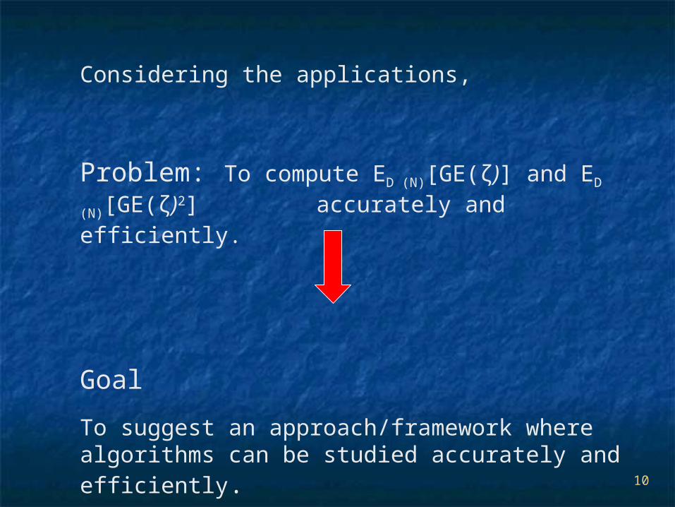
Considering the applications,

Problem: To compute ED (N)[GE(ζ)] and ED

(N)[GE(ζ)2]

accurately and efficiently.

Goal

To suggest an approach/framework where algorithms can be studied accurately and efficiently.

11

Roadmap

Strategies to compute moments efficiently and accurately.

• Example, Naïve Bayes Classifier (NBC).

Analysis of model selection measures.

• Example, behavior of cross-validation.

Conclusion.

12

Note:

Formulas are shown with sums but results are also applicable in the continuous domain.

Reasons:

Its relatively easier to understand.

Machinery to compute finite sums efficiently and accurately is considerably limited as compared to

computing integrals.

13

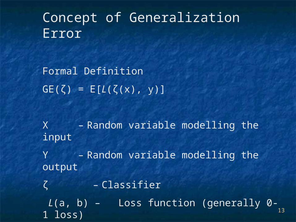
Concept of Generalization Error

Formal Definition

GE(ζ) = E[L(ζ(x), y)]

X – Random variable modelling the input

Y – Random variable modelling the output

ζ – Classifier

L(a, b) – Loss function (generally 0-1 loss)

Assumption: Samples are independent and identically distributed (i.i.d.).

14

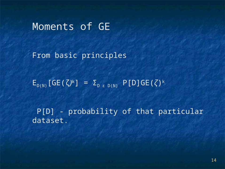
Moments of GE

From basic principles

ED(N)[GE(ζ)k] = ΣD ϵ D(N) P[D]GE(ζ)k

P[D] - probability of that particular dataset.

15

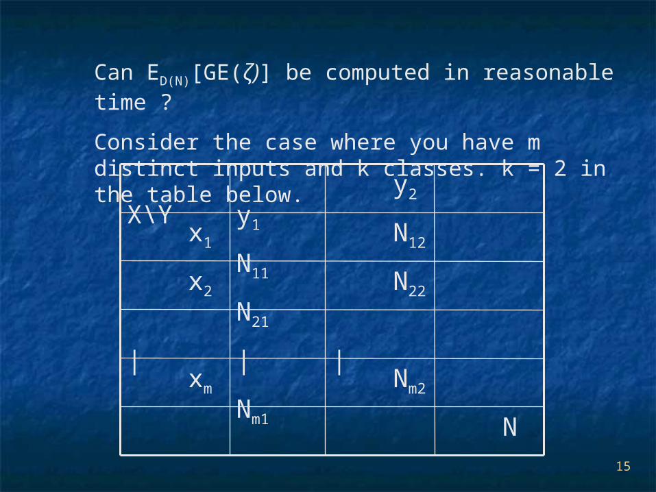
Can ED(N)[GE(ζ)] be computed in reasonable time ?

Consider the case where you have m distinct inputs and k classes. k = 2 in the table below.

N

Nm2 Nm1 xm

| | |

N22 N21 x2

N12 N11 x1

y2 y1 X\Y

16

ED(N)[GE(ζ)] = P[D1]GE(ζ1) + P[D2]GE(ζ2) + ...

Number of possible datasets = O(Nmk-1)

Size of the probabilities = O(mk)

TOO MANY !!!

17

Optimizations

Number of terms

Calculation of each term

Lets consider the first optimization…

18

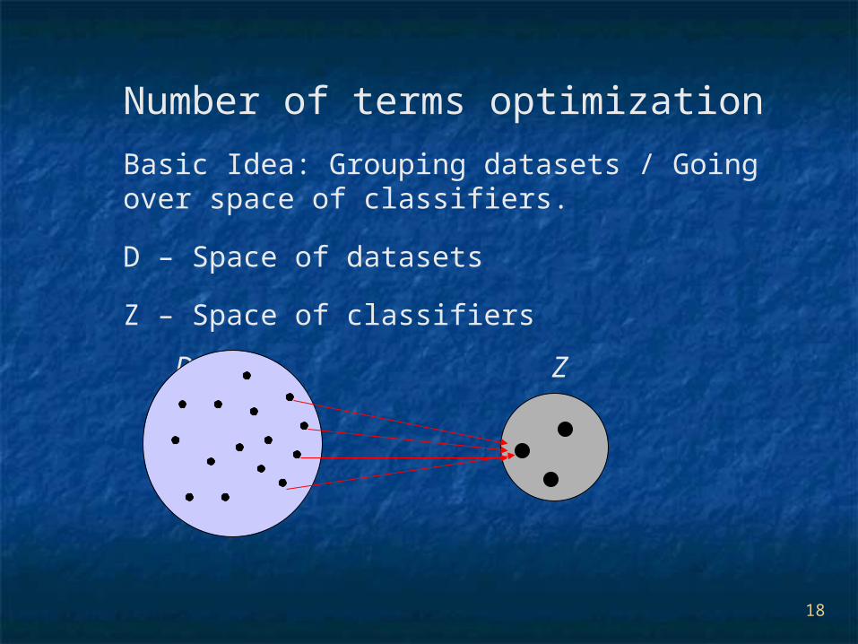
Number of terms optimization

Basic Idea: Grouping datasets / Going over space of classifiers.

D – Space of datasets

Z – Space of classifiers

D Z

19

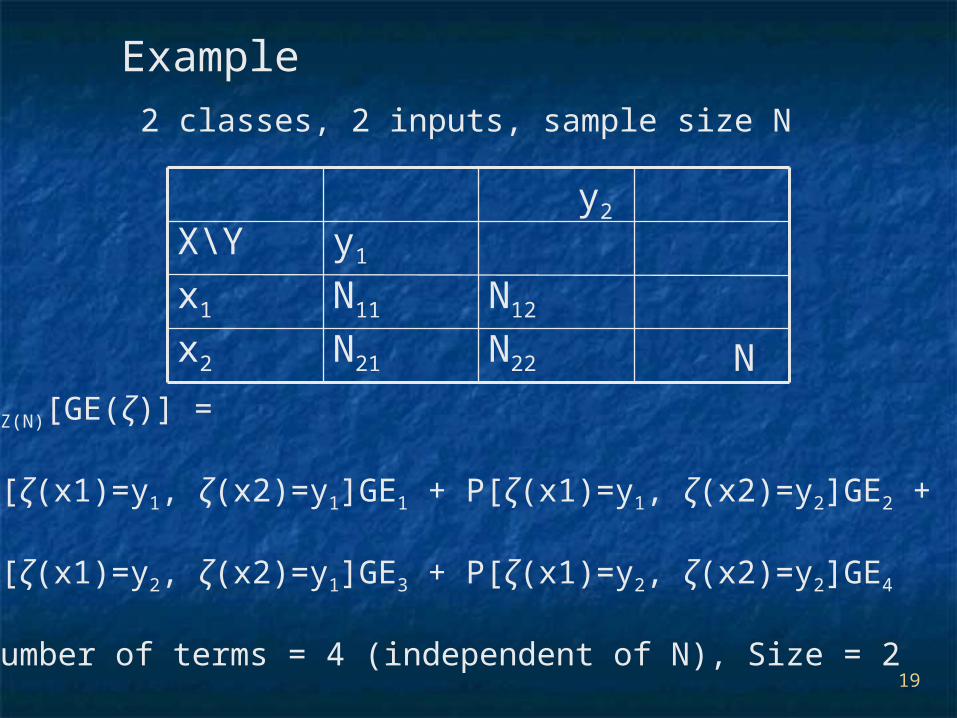
Example

2 classes, 2 inputs, sample size N

N

N22 N21 x2

N12 N11 x1

y2 y1 X\Y

EZ(N)[GE(ζ)] =

P[ζ(x1)=y1, ζ(x2)=y1]GE1 + P[ζ(x1)=y1, ζ(x2)=y2]GE2 +

P[ζ(x1)=y2, ζ(x2)=y1]GE3 + P[ζ(x1)=y2, ζ(x2)=y2]GE4

Number of terms = 4 (independent of N), Size = 2

20

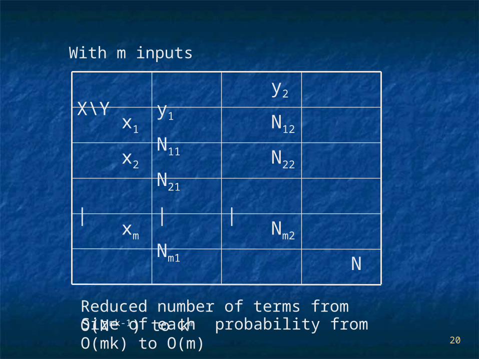
With m inputs

N

Nm2 Nm1 xm

| | |

N22 N21 x2

N12 N11 x1

y2 y1 X\Y

Reduced number of terms from O(Nmk-1) to km

Size of each probability from O(mk) to O(m)

21

Number of terms = O(mk) for the first moment.

Need to focus only on local behaviour of the classifiers.

Note: Probabilities after summation over y in the first moment are conditionals given x and analogously for the second moment probabilities are conditioned on x and x’.

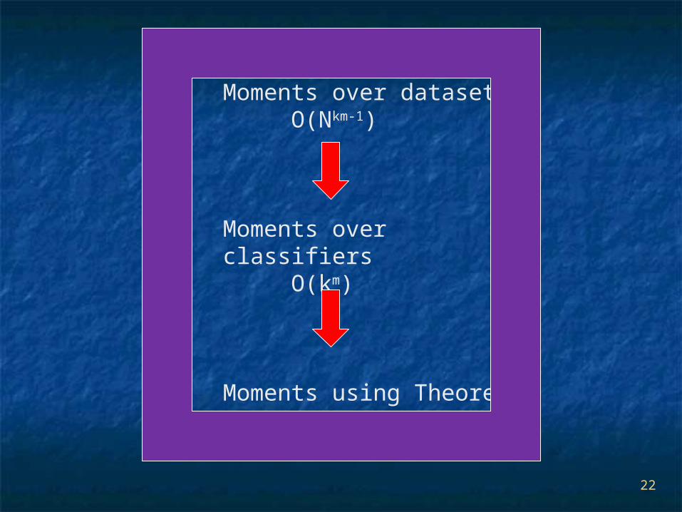
22

Moments over datasetsO(Nkm-1)

Moments over classifiersO(km)

Moments using Theorem 1O(mk)

23

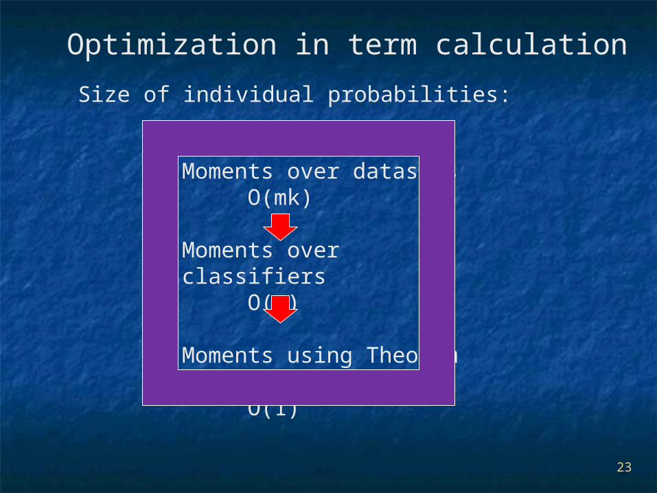
Optimization in term calculation

Moments over datasetsO(mk)

Moments over classifiersO(m)

Moments using Theorem 1O(1)

Size of individual probabilities:

24

Now we will talk about efficiently computing,

P[ζ(x)=y] and P[ζ(x)=y, ζ’(x’)=y’]

25

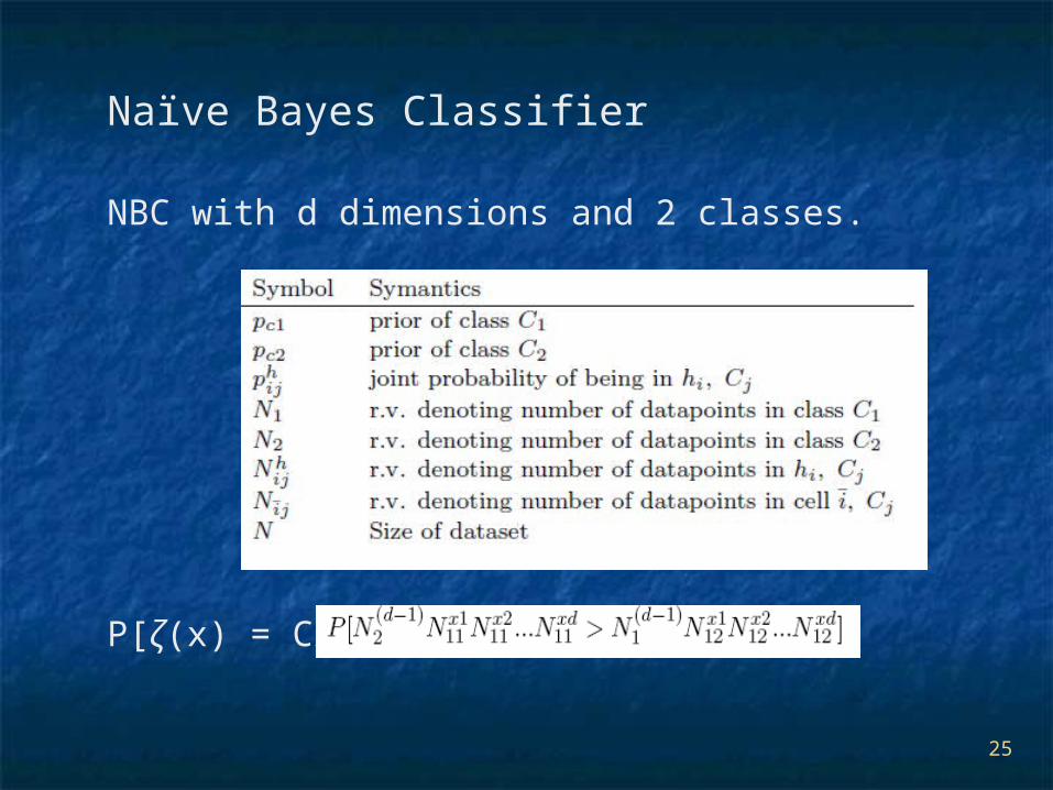
Naïve Bayes Classifier

NBC with d dimensions and 2 classes.

P[ζ(x) = C1] =

26

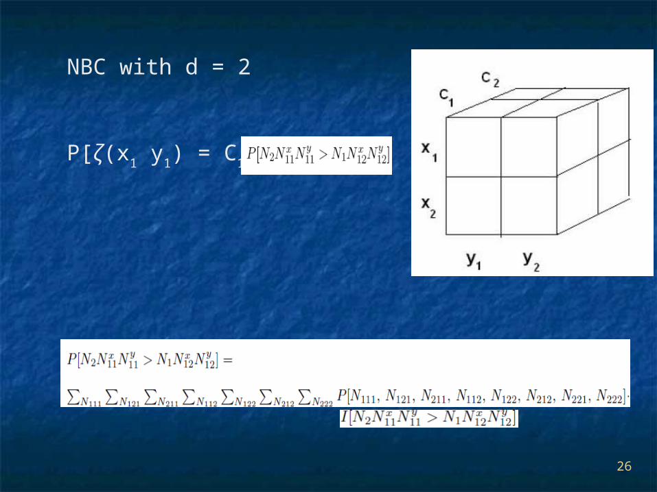
NBC with d = 2

P[ζ(x1 y

1) = C

1] =

27

Exact Computation TOO expensive

Solution: Approximate the probabilities.

Notice: The condition in the probabilities are

polynomials in the cell random variables.

28

We let

Need to find

Moment Generating Function (MGF) of multinomial known.

How does this help ?

29

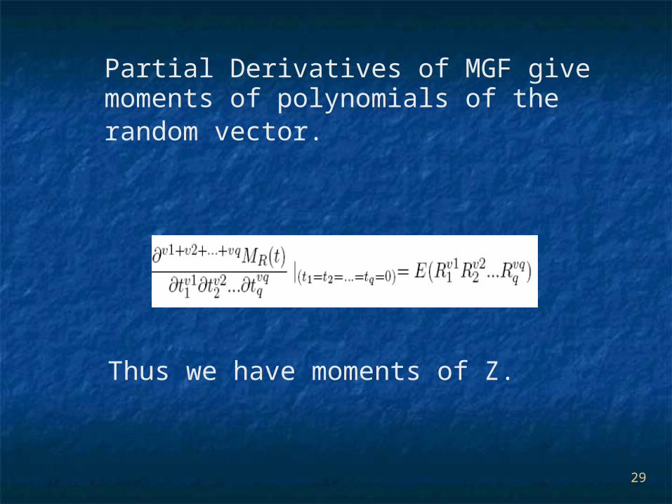
Partial Derivatives of MGF give moments of polynomials of the random vector.

Thus we have moments of Z.

30

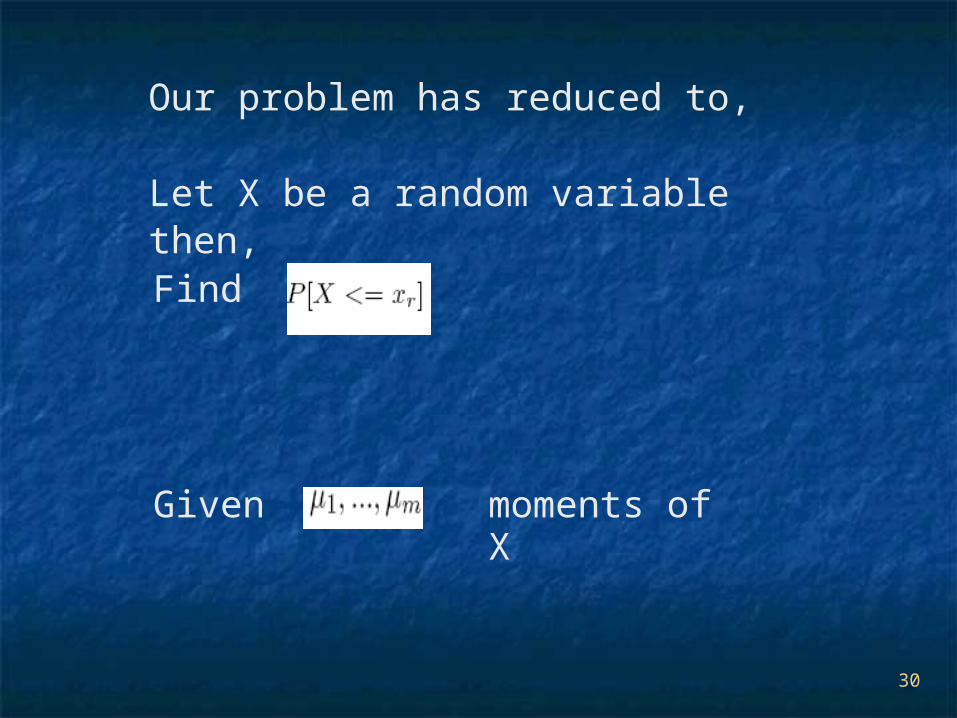
Our problem has reduced to,

Find

Given moments of X

Let X be a random variable then,

31

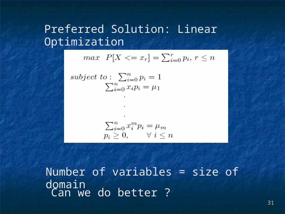
Preferred Solution: Linear Optimization

Number of variables = size of domain

Can we do better ?

32

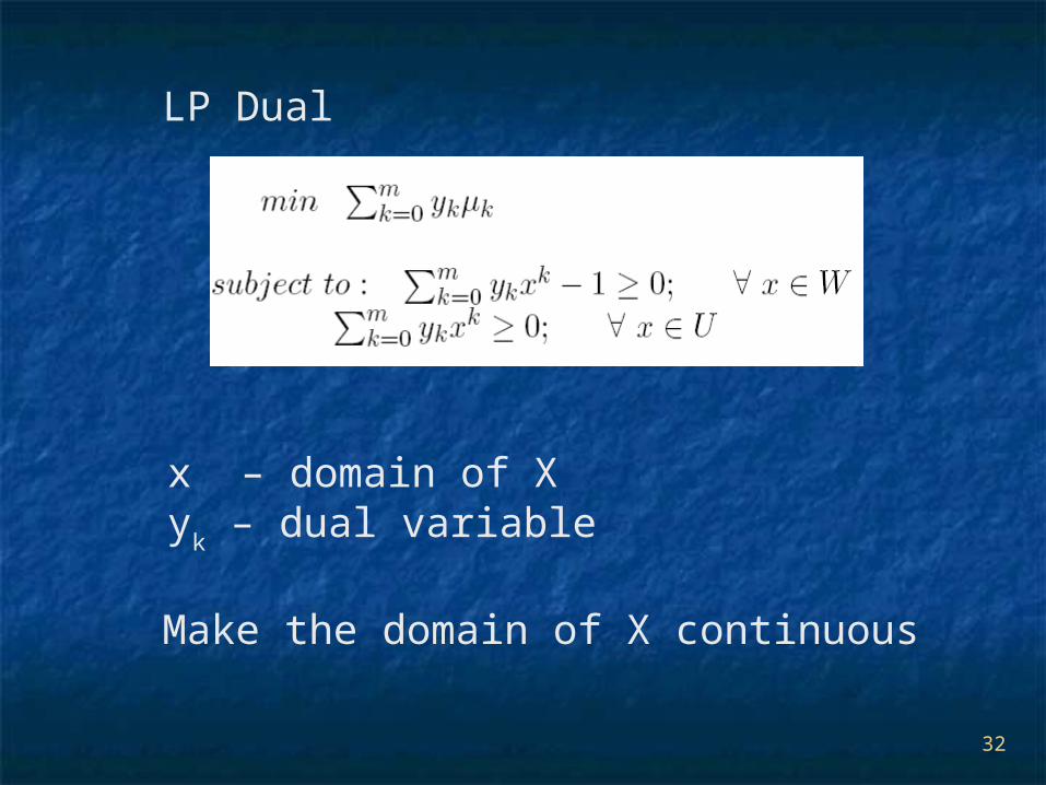
LP Dual

x – domain of Xy

k – dual variable

Make the domain of X continuous

33

X – continuous in [-a,a]

Have 2 polynomials rather than multiple constraints

Bounds still valid.

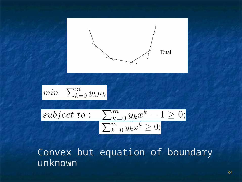
34

Convex but equation of boundary unknown

35

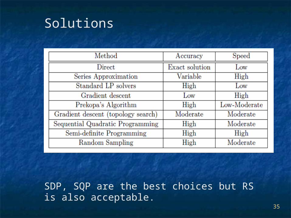
Solutions

SDP, SQP are the best choices but RS is also acceptable.

36

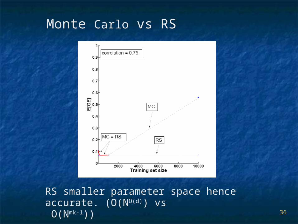
Monte Carlo vs RS

RS smaller parameter space hence accurate. (O(NO(d)) vs O(Nmk-1))

37

RS better than MC even for some other algorithms…

In fact for Random decision trees RS was more accurate than MC-10 and Breimans bounds based on strength and correlation.

(Probabilistic Characterization of Random Decision trees, JMLR 2008)

38

Collapsing Joint Cumulative Probabilities

39

Optimization in term computation

Message: Use SDP or SQP for high accuracy and efficiency wherever possible. Use RS in other scenarios when the parameter space of the probabilities is smaller than the space of datasets/classifiers.

40

Summary

We reduced number of terms.

We speeded up the computation of each term.

Totally intractable to tractable.

41

Other Classification Algorithms

Decision tree algorithms

where p indexes all allowed paths in the tree, ct(pathpy) is the number of inputs in pathp with class label y.

42

Other Classification Algorithms

K Nearest Neighbor algorithm (KNN)

where Q is the set of all possible KNNs of x and c(q,y) is the number of KNNs in class y.

43

Analysis of model selection measures

Hold out set (HE)

Cross validation (CE)

Leave one out (special case of CE)

44

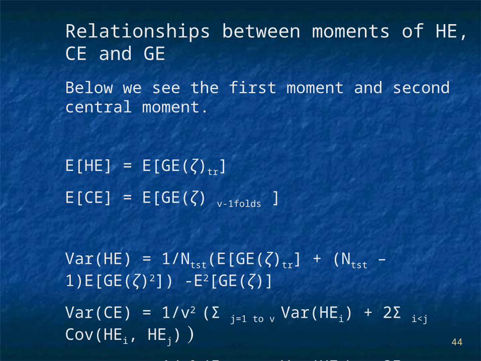
Relationships between moments of HE, CE and GE

Below we see the first moment and second central moment.

E[HE] = E[GE(ζ)tr]

E[CE] = E[GE(ζ) v-1folds ]

Var(HE) = 1/Ntst(E[GE(ζ)tr] + (Ntst – 1)E[GE(ζ)2]) -E2[GE(ζ)]

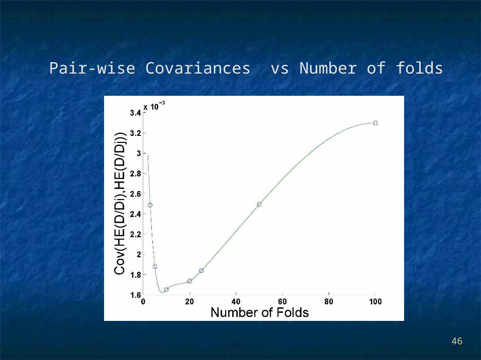
Var(CE) = 1/v2 (Σ j=1 to v Var(HEi) + 2Σ i<j Cov(HEi, HEj) )

= 1/v2 (Σ j=1 to v Var(HEi) + 2Σ i<jE[GEiGEj]-

E[GEi]E[GEj] )

For proofs and relationships read the TKDD paper.

45

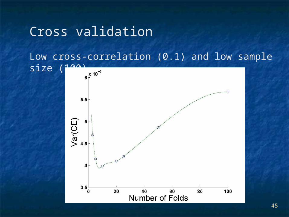
Cross validation

Low cross-correlation (0.1) and low sample size (100).

46

Pair-wise Covariances vs Number of folds

47

Able to explain trends of cross-validation w.r.t.

different sample sizes and

different levels of correlation between input attributes and class labels

based on the observation of the 3 algorithms.

48

Convergence in real dataset sizes

49

Conclusion

Challenges:

Expressions can be tedious to figure out.

More scalable solutions need to be designed.

however we feel …

To accurately study behavior of learning algorithms for finite sample sizes the approach has merit.

50

THANK YOU !