Script for the Course Machine Lab ISE Master

Study of centrifugal pump operation in different arrangements by experimental methods

a) General about centrifugal pumps b) Parallel and series operation of pumps c) Example for parallel and series operation d) Tasks for the Lab e) Description of the test facility f) Report g) Literature

a) General about centrifugal pumps 1 General about centrifugal pumps 4

1.1 Range of application of centrifugal pumps ................................................................... 4 1.2 Impeller forms and pumping designs ............................................................................ 4

2 Theoretical bases 6

2.1 Speed conditions at the impeller ................................................................................... 6 2.2 Compression in impeller and peeler.............................................................................. 8 2.3 Determination of the delivery head............................................................................. 10

2.3.1 Influence of the finite number of blades ............................................................ 10 2.3.2 Blade angle β2

* ................................................................................................... 12 2.4 Losses and efficiencies................................................................................................ 13 2.5 Operating performance................................................................................................ 14

2.5.1 Centrifugal pump characteristics........................................................................ 15 2.5.2 Similarity laws.................................................................................................... 19 2.5.3 Operating point of the pump .............................................................................. 21

2.5.4 Regulation of centrifugal pump plants 22

Bibliography 1. Bohl, W.: Strömungsmaschinen Bd. 1 und 2 Vogel-Verlag 2. Bohl, W.; Mathieu, W.: Laborversuche an Kraft- und

Arbeitsmaschinen Hanser-Verlag, 1975

3. Schulz, H.: Die Pumpen Springer-Verlag, 1977 4. KSB: Kreiselpumpenlexikon KSB-AG, Frankenthal, 1989 5. Pfleiderer, C.; Petermann, H.: Strömungsmaschinen Springer-Verlag, 1990 6. Sigloch, H.: Strömungsmaschinen Hanser-Verlag, 1993 7. SIHI: Grundlagen für die Planung von Kreiselpumpenanlagen

SIHI-Halberg, Ludwigshafen, 1978 8. Spengler, H.: Technisches Handbuch Pumpen Technik-Verlag, 1987 9. Stepanoff, A.: Radial- und Axialpumpen

Springer-Verlag, 1959

10. Troskolanski, A.T.; Lazarkiewicz, S.: Kreiselpumpen Birkhäuser-Verlag, 1976 11. Sulzer: Kreiselpumpen Handbuch Vulkan-Verlag, 1990 12. Benra, F.-K.: Hydraulische Strömungsmaschinen

Vorlesungsskript, Universität Duisburg-Essen

13. Benra, F.-K.: Berechnung und Konstruktion von Strömungsmaschinen Vorlesungsskript, Universität Duisburg-Essen

14. Simon, H.: Strömungsmaschinen I Vorlesungsskript, Universität Duisburg-Essen

15. Simon, H.: Strömungsmaschinen II Vorlesungsskript, Universität Duisburg-Essen

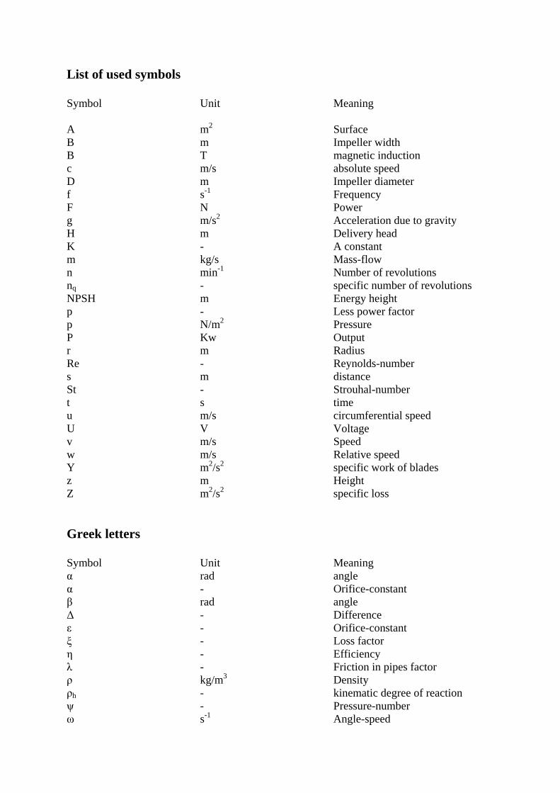
List of used symbols Symbol Unit Meaning A m2 Surface B m Impeller width B T magnetic induction c m/s absolute speed D m Impeller diameter f s-1 Frequency

F N Power g m/s2 Acceleration due to gravity H m Delivery head K - A constant m kg/s Mass-flow n min-1 Number of revolutions nq - specific number of revolutions NPSH m Energy height p - Less power factor p N/m2 Pressure P Kw Output r m Radius Re - Reynolds-number s m distance St - Strouhal-number t s time u m/s circumferential speed U V Voltage v m/s Speed w m/s Relative speed Y m2/s2 specific work of blades z m Height Z m2/s2 specific loss Greek letters Symbol Unit Meaning α rad angle α - Orifice-constant β rad angle Δ - Difference ε - Orifice-constant ξ - Loss factor η - Efficiency λ - Friction in pipes factor ρ kg/m3 Density ρh - kinematic degree of reaction ψ - Pressure-number ω s-1 Angle-speed

Indices a Impeller a A Plant b Impeller b d Torque dyn dynamic D Pressure-site el electric erf needed h hydraulic i internal i optional K Clutch m mechanic max. maximum min. minimum M measured value N Nominal size Opt. Optimum P Pump r friction-caused R Friction stat static S Suction-site Sch Vertex Sch blade Sp Gap th theoretic u in circumferential direction vorh given V Loss 0 at zero delivering 1 Stage 1, Place 2 Stage 2, Place ∞ Infinite, environment

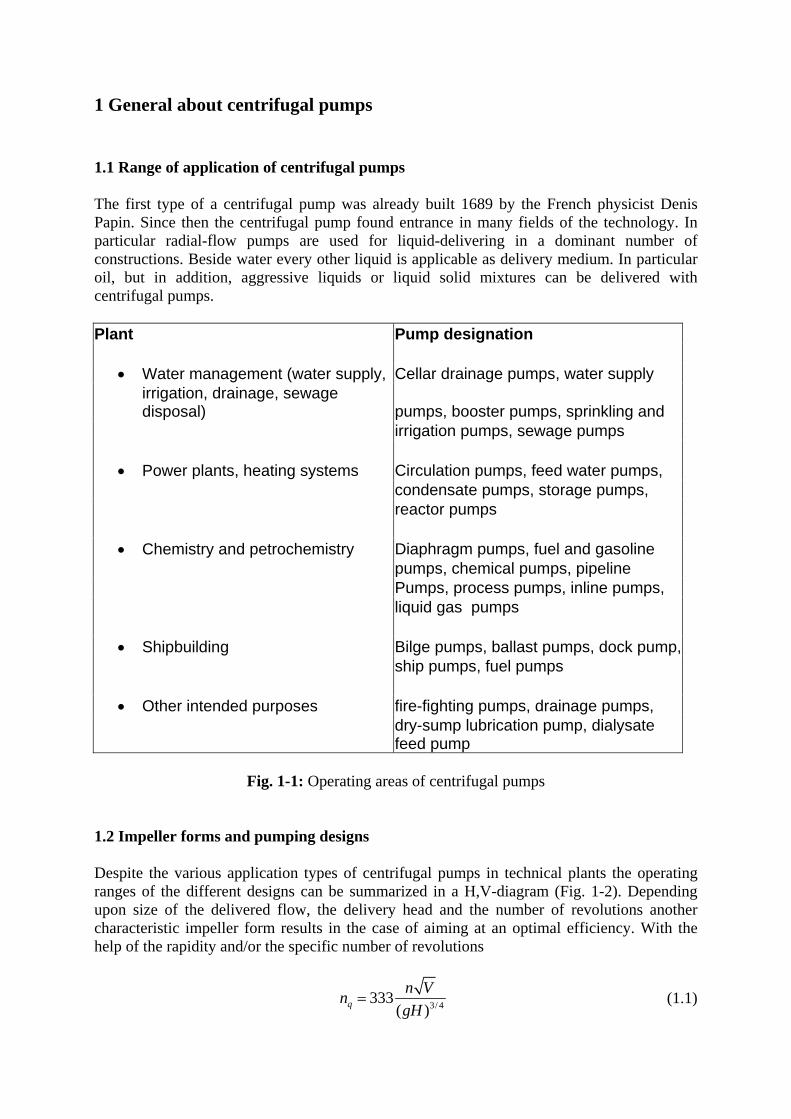
1 General about centrifugal pumps 1.1 Range of application of centrifugal pumps The first type of a centrifugal pump was already built 1689 by the French physicist Denis Papin. Since then the centrifugal pump found entrance in many fields of the technology. In particular radial-flow pumps are used for liquid-delivering in a dominant number of constructions. Beside water every other liquid is applicable as delivery medium. In particular oil, but in addition, aggressive liquids or liquid solid mixtures can be delivered with centrifugal pumps. Plant Pump designation

• Water management (water supply, Cellar drainage pumps, water supply irrigation, drainage, sewage disposal) pumps, booster pumps, sprinkling and

irrigation pumps, sewage pumps

• Power plants, heating systems Circulation pumps, feed water pumps, condensate pumps, storage pumps, reactor pumps

• Chemistry and petrochemistry Diaphragm pumps, fuel and gasoline pumps, chemical pumps, pipeline Pumps, process pumps, inline pumps, liquid gas pumps

• Shipbuilding Bilge pumps, ballast pumps, dock pump, ship pumps, fuel pumps

• Other intended purposes fire-fighting pumps, drainage pumps,

dry-sump lubrication pump, dialysate feed pump

Fig. 1-1: Operating areas of centrifugal pumps

1.2 Impeller forms and pumping designs Despite the various application types of centrifugal pumps in technical plants the operating ranges of the different designs can be summarized in a H,V-diagram (Fig. 1-2). Depending upon size of the delivered flow, the delivery head and the number of revolutions another characteristic impeller form results in the case of aiming at an optimal efficiency. With the help of the rapidity and/or the specific number of revolutions

3/ 4333( )q

n VngH

= (1.1)

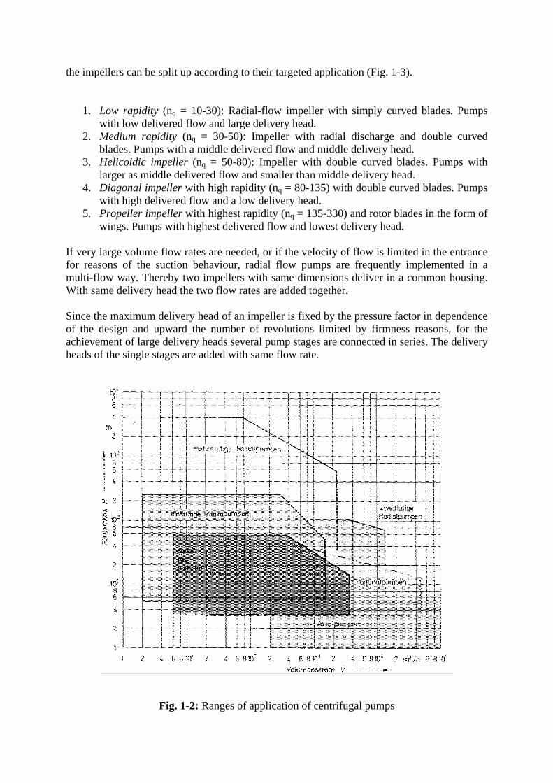
the impellers can be split up according to their targeted application (Fig. 1-3).

1. Low rapidity (nq = 10-30): Radial-flow impeller with simply curved blades. Pumps with low delivered flow and large delivery head.

2. Medium rapidity (nq = 30-50): Impeller with radial discharge and double curved blades. Pumps with a middle delivered flow and middle delivery head.

3. Helicoidic impeller (nq = 50-80): Impeller with double curved blades. Pumps with larger as middle delivered flow and smaller than middle delivery head.

4. Diagonal impeller with high rapidity (nq = 80-135) with double curved blades. Pumps with high delivered flow and a low delivery head.

5. Propeller impeller with highest rapidity (nq = 135-330) and rotor blades in the form of wings. Pumps with highest delivered flow and lowest delivery head.

If very large volume flow rates are needed, or if the velocity of flow is limited in the entrance for reasons of the suction behaviour, radial flow pumps are frequently implemented in a multi-flow way. Thereby two impellers with same dimensions deliver in a common housing. With same delivery head the two flow rates are added together. Since the maximum delivery head of an impeller is fixed by the pressure factor in dependence of the design and upward the number of revolutions limited by firmness reasons, for the achievement of large delivery heads several pump stages are connected in series. The delivery heads of the single stages are added with same flow rate.

Fig. 1-2: Ranges of application of centrifugal pumps

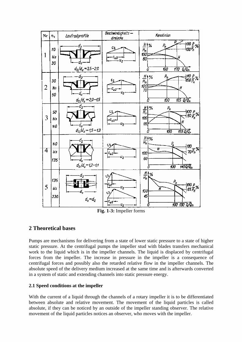
Fig. 1-3: Impeller forms

2 Theoretical bases Pumps are mechanisms for delivering from a state of lower static pressure to a state of higher static pressure. At the centrifugal pumps the impeller stud with blades transfers mechanical work to the liquid which is in the impeller channels. The liquid is displaced by centrifugal forces from the impeller. The increase in pressure in the impeller is a consequence of centrifugal forces and possibly also the retarded relative flow in the impeller channels. The absolute speed of the delivery medium increased at the same time and is afterwards converted in a system of static and extending channels into static pressure energy. 2.1 Speed conditions at the impeller With the current of a liquid through the channels of a rotary impeller it is to be differentiated between absolute and relative movement. The movement of the liquid particles is called absolute, if they can be noticed by an outside of the impeller standing observer. The relative movement of the liquid particles notices an observer, who moves with the impeller.

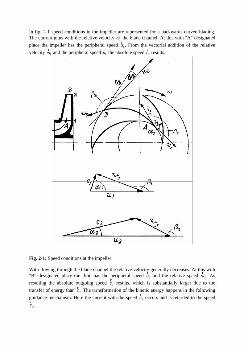
In fig. 2-1 speed conditions in the impeller are represented for a backwards curved blading. The current joins with the relative velocity 1ω

r the blade channel. At this with "A" designated

place the impeller has the peripheral speed 1ur . From the vectorial addition of the relative velocity 1ω

r and the peripheral speed 1ur the absolute speed 1cr results.

Fig. 2-1: Speed conditions at the impeller With flowing through the blade channel the relative velocity generally decreases. At this with "B" designated place the fluid has the peripheral speed 2ur and the relative speed 2ω

r . As resulting the absolute outgoing speed 2cr results, which is substantially larger due to the transfer of energy than 1cr . The transformation of the kinetic energy happens in the following guidance mechanism. Here the current with the speed 2cr occurs and is retarded to the speed

3cr .

2.2 Compression in impeller and peeler The work transferred in the impeller to the liquid is converted to pressure energy on the one hand by the increase of the circumferential speed from u1 to u2 and on the other hand by the delay of the current in impeller and peeler. In order to be able to determine the compression in the impeller and in the peeler, one makes the assumption that all liquid particles follow accurately the course of the rotor blades (Blade-congruent current). Thus the flow conditions (pressure and speed) are alike in each case along concentric circles around the perpendicularly arranged wheel axle. This condition can be fulfilled by the assumption of infinitely many and infinitely thin blades. Further the transformation from speed energy in pressure energy should happen in the blade channels and the repeating-condition ( 3c c1=

r r ) should be fulfilled. The increase in pressure from the work of centrifugal forces can be determined, if a mass particle of the pumping medium is regarded, which is limited by the lateral surfaces of two cylinders with the radii r and r+dr as well as two neighbouring blades and the wheel walls of cover- and wheel disk (Fig. 2-2a). Thus the centrifugal force of the mass particle can be expressed as follows:

2dF dA dr rρ ω′ = ⋅ ⋅ ⋅ ⋅ 2.1)

From this follows for the increase in pressure:

2dp rdrρω= (2.2)

If one names with

2dp dY rdrωρ ∞

′= = (2.3)

the specific flow work of centrifugal forces, then the work portion from centrifugal forces can be determined by integration along the radius.

1

11 p

p

p pY dpρ ρ

∞ ∞∞

−′ = =∫ (2.4)

2

1

2 2 22 2 2 1 2 1

2 2r

r

r r u uY rdrω ω∞

2− −′ = = =∫ (2.5)

As a result of the introduction of acceleration due to gravity the delivery head portion arises due to centrifugal forces to:

2 21 2 1

2Y p p u uHg g gρ∞ ∞

∞

′ − −′ = = = (2.6)

The increase in pressure from the delay of the relative velocity w can be derived by fig. 2-2b from the dynamic Basic Law:

ddF dA dsdtωρ′′ = − ⋅ ⋅ ⋅ (2.7)

Thereby dw is negative since w decreases with rising pressure. With ds/dt = w and dp = dF´´/dA can be written:

dp dρω ω= − (2.8)

Names one this time

dp dY dω ωρ ∞

′′= = − (2.9)

the specific flow work from the delay of the relative velocity, then this work portion can be determined by integration along the entire flow channel:

1 pp p

p

p pY dp

ρ ρ∞

∞

∞ ∞∞

−′′ = =∫ (2.10)

2

1

2 21 2

2Y d

ω

ω

ω ωω ω∞ ∞∞

−′′ = − =∫ (2.11)

With acceleration due to gravity the delivery head results

2 21 2

2pp p

Hg g

ω ωρ∞ ∞ ∞

∞

− −′′ = = (2.12)

With fig. 2-2c for the transformation of the speed energy in the peeler accordingly derives:

2 22 2 1

2pp p c cH

g gρ∞ ∞

∞

− −′′′ = = (2.13)

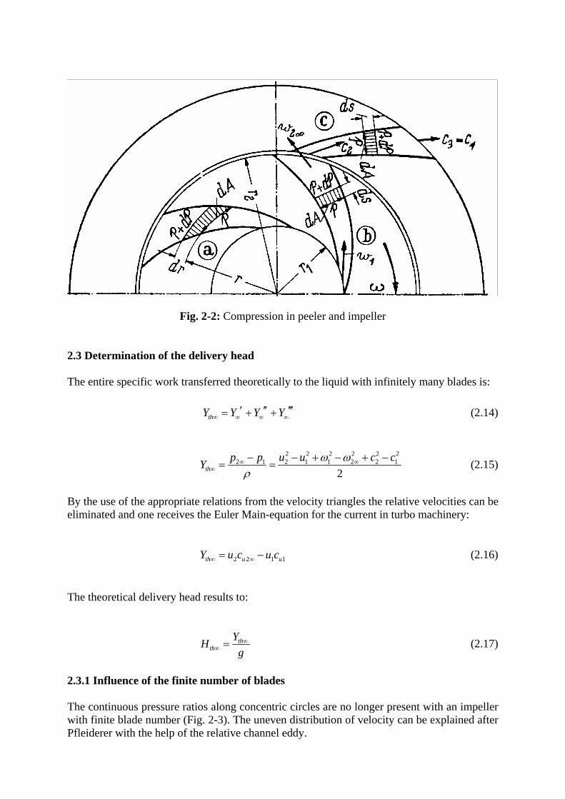
Fig. 2-2: Compression in peeler and impeller 2.3 Determination of the delivery head The entire specific work transferred theoretically to the liquid with infinitely many blades is:

thY Y Y Y∞ ∞ ∞ ∞′ ′′ ′′′= + + (2.14)

2 2 2 2 22 1 2 1 1 2 2

2th

21p p u u c cY ω ω

ρ∞ ∞

∞

− − + − + −= = (2.15)

By the use of the appropriate relations from the velocity triangles the relative velocities can be eliminated and one receives the Euler Main-equation for the current in turbo machinery:

2 2 1 1th u uY u c u c∞ ∞= − (2.16) The theoretical delivery head results to:

thth

YHg∞

∞ = (2.17)

2.3.1 Influence of the finite number of blades The continuous pressure ratios along concentric circles are no longer present with an impeller with finite blade number (Fig. 2-3). The uneven distribution of velocity can be explained after Pfleiderer with the help of the relative channel eddy.

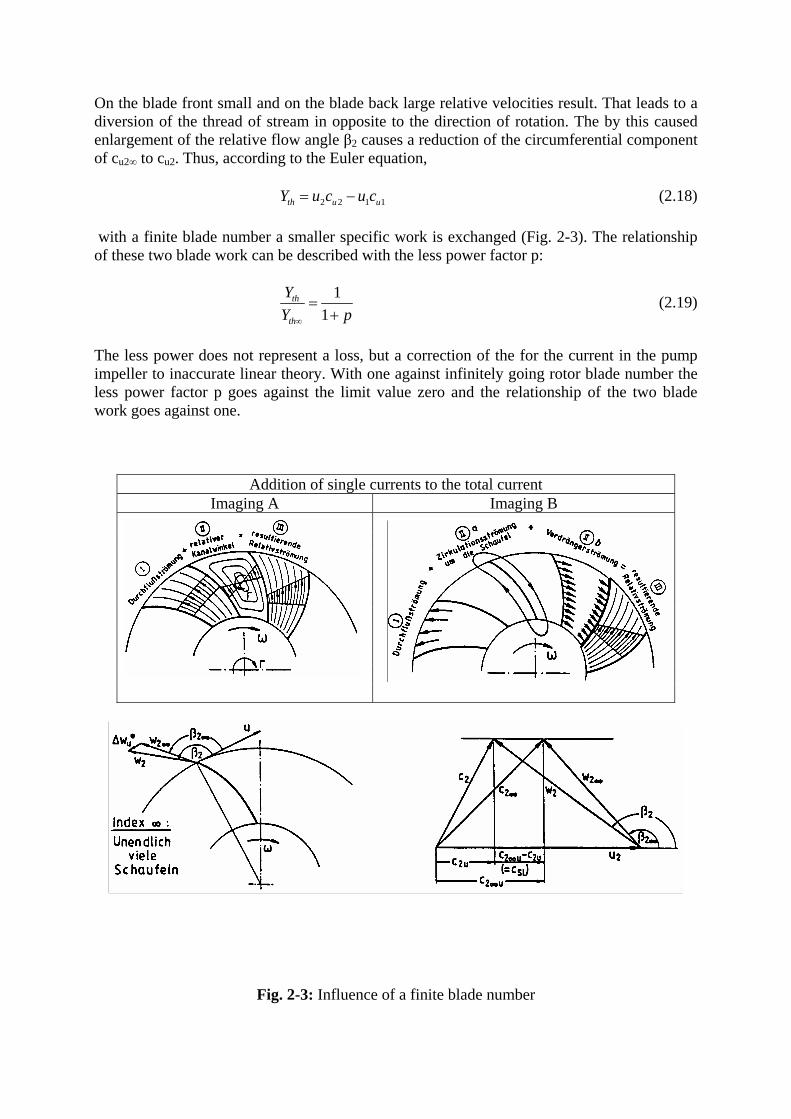
On the blade front small and on the blade back large relative velocities result. That leads to a diversion of the thread of stream in opposite to the direction of rotation. The by this caused enlargement of the relative flow angle β2 causes a reduction of the circumferential component of cu2∞ to cu2. Thus, according to the Euler equation,

2 2 1 1th u uY u c u c= − (2.18) with a finite blade number a smaller specific work is exchanged (Fig. 2-3). The relationship of these two blade work can be described with the less power factor p:

11

th

th

YY p∞

=+

(2.19)

The less power does not represent a loss, but a correction of the for the current in the pump impeller to inaccurate linear theory. With one against infinitely going rotor blade number the less power factor p goes against the limit value zero and the relationship of the two blade work goes against one.

Addition of single currents to the total current Imaging A Imaging B

Fig. 2-3: Influence of a finite blade number

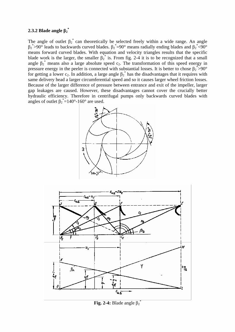
2.3.2 Blade angle β2*

The angle of outlet β2

* can theoretically be selected freely within a wide range. An angle β2

*>90° leads to backwards curved blades. β2*=90° means radially ending blades and β2

*<90° means forward curved blades. With equation and velocity triangles results that the specific blade work is the larger, the smaller β2

* is. From fig. 2-4 it is to be recognized that a small angle β2

* means also a large absolute speed c2. The transformation of this speed energy in pressure energy in the peeler is connected with substantial losses. It is better to chose β2

*>90° for getting a lower c2. In addition, a large angle β2

* has the disadvantages that it requires with same delivery head a larger circumferential speed and so it causes larger wheel friction losses. Because of the larger difference of pressure between entrance and exit of the impeller, larger gap leakages are caused. However, these disadvantages cannot cover the crucially better hydraulic efficiency. Therefore in centrifugal pumps only backwards curved blades with angles of outlet β2

*=140°-160° are used.

Fig. 2-4: Blade angle β2

*

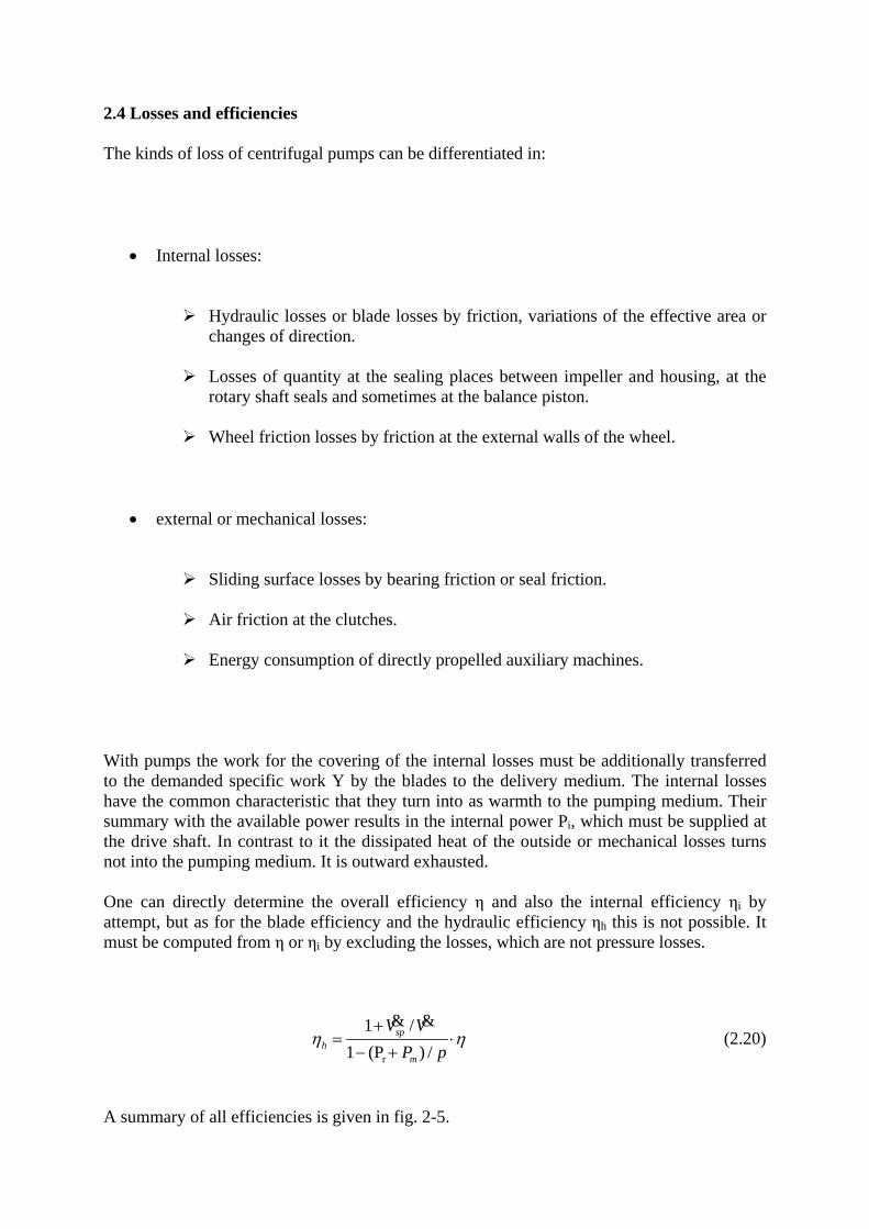
2.4 Losses and efficiencies The kinds of loss of centrifugal pumps can be differentiated in:

• Internal losses:

Hydraulic losses or blade losses by friction, variations of the effective area or changes of direction.

Losses of quantity at the sealing places between impeller and housing, at the

rotary shaft seals and sometimes at the balance piston.

Wheel friction losses by friction at the external walls of the wheel.

• external or mechanical losses:

Sliding surface losses by bearing friction or seal friction.

Air friction at the clutches.

Energy consumption of directly propelled auxiliary machines. With pumps the work for the covering of the internal losses must be additionally transferred to the demanded specific work Y by the blades to the delivery medium. The internal losses have the common characteristic that they turn into as warmth to the pumping medium. Their summary with the available power results in the internal power Pi, which must be supplied at the drive shaft. In contrast to it the dissipated heat of the outside or mechanical losses turns not into the pumping medium. It is outward exhausted. One can directly determine the overall efficiency η and also the internal efficiency ηi by attempt, but as for the blade efficiency and the hydraulic efficiency ηh this is not possible. It must be computed from η or ηi by excluding the losses, which are not pressure losses.

r

1 /1 (P ) /

sph

m

V VP p

η η+

=− +

& &⋅ (2.20)

A summary of all efficiencies is given in fig. 2-5.

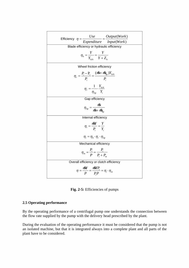
Efficiency ( )

( )Use Output Work

Expenditure Input Workη = =

Blade efficiency or hydraulic efficiency

hSch h

Y YY Y Z

η = =+

Wheel friction efficiency

r ( )P Sp Schir

i i

m m YPP P

η+−

= =& &

1 Schr

Sp i

YY

ηη

= ⋅

Gap efficiency

SpSp

mm m

η =+

&& &

Internal efficiency

ii i

mY YP Y

η = =&

i h r Spη η η η= ⋅ ⋅

Mechanical efficiency

i im

i m

P PP P P

η = =+

Overall efficiency or clutch efficiency

ii m

i

mYPmYP PP

η η η= = = ⋅&&

Fig. 2-5: Efficiencies of pumps 2.5 Operating performance By the operating performance of a centrifugal pump one understands the connection between the flow rate supplied by the pump with the delivery head prescribed by the plant. During the evaluation of the operating performance it must be considered that the pump is not an isolated machine, but that it is integrated always into a complete plant and all parts of the plant have to be considered.

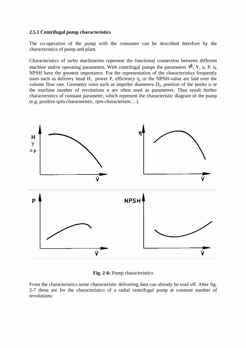
2.5.1 Centrifugal pump characteristics The co-operation of the pump with the consumer can be described therefore by the characteristics of pump and plant. Characteristics of turbo machineries represent the functional connection between different machine and/or operating parameters. With centrifugal pumps the parameters V&, Y, n, P, η, NPSH have the greatest importance. For the representation of the characteristics frequently sizes such as delivery head H, power P, efficiency η, or the NPSH-value are laid over the volume flow rate. Geometry sizes such as impeller diameters D2, position of the peeler α or the machine number of revolutions n are often used as parameters. Thus result further characteristics of constant parameter, which represent the characteristic diagram of the pump (e.g. positive spin-characteristic, rpm-characteristic…).

Fig. 2-6: Pump characteristics

From the characteristics some characteristic delivering data can already be read off. After fig. 2-7 these are for the characteristics of a radial centrifugal pump at constant number of revolutions:

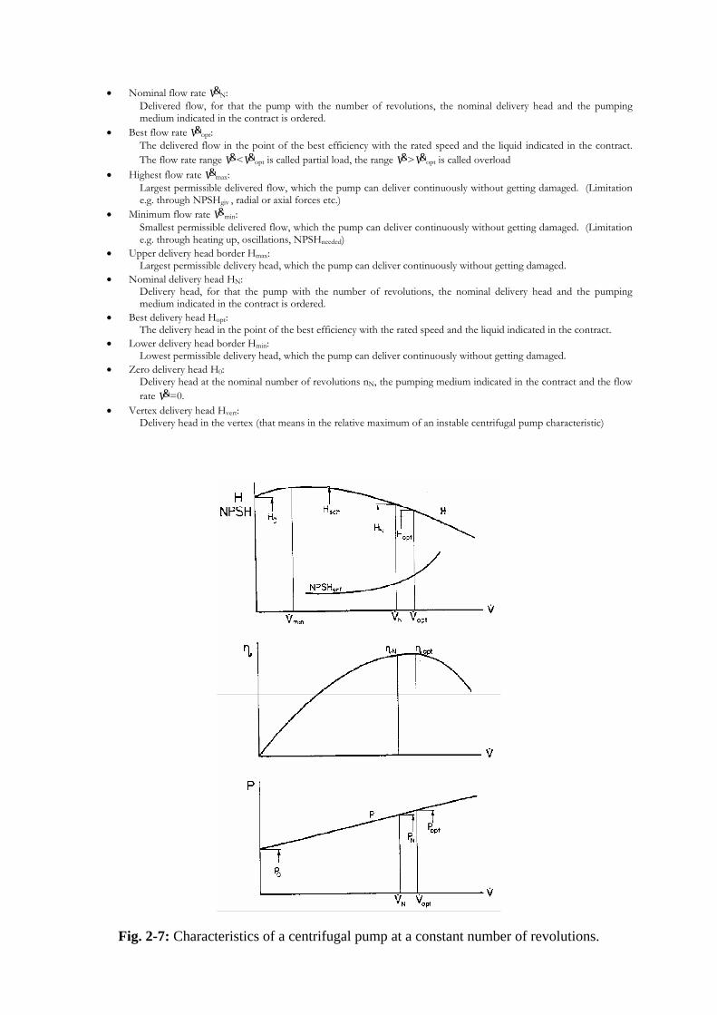
• Nominal flow rate V&N: Delivered flow, for that the pump with the number of revolutions, the nominal delivery head and the pumping medium indicated in the contract is ordered.

• Best flow rate V&opt: The delivered flow in the point of the best efficiency with the rated speed and the liquid indicated in the contract. The flow rate range V&<V&opt is called partial load, the range V&>V&opt is called overload

• Highest flow rate V&max: Largest permissible delivered flow, which the pump can deliver continuously without getting damaged. (Limitation e.g. through NPSHgiv , radial or axial forces etc.)

• Minimum flow rate V&min: Smallest permissible delivered flow, which the pump can deliver continuously without getting damaged. (Limitation e.g. through heating up, oscillations, NPSHneeded)

• Upper delivery head border Hmax: Largest permissible delivery head, which the pump can deliver continuously without getting damaged.

• Nominal delivery head HN: Delivery head, for that the pump with the number of revolutions, the nominal delivery head and the pumping medium indicated in the contract is ordered.

• Best delivery head Hopt: The delivery head in the point of the best efficiency with the rated speed and the liquid indicated in the contract.

• Lower delivery head border Hmin: Lowest permissible delivery head, which the pump can deliver continuously without getting damaged.

• Zero delivery head H0: Delivery head at the nominal number of revolutions nN, the pumping medium indicated in the contract and the flow rate V&=0.

• Vertex delivery head Hvert: Delivery head in the vertex (that means in the relative maximum of an instable centrifugal pump characteristic)

Fig. 2-7: Characteristics of a centrifugal pump at a constant number of revolutions.

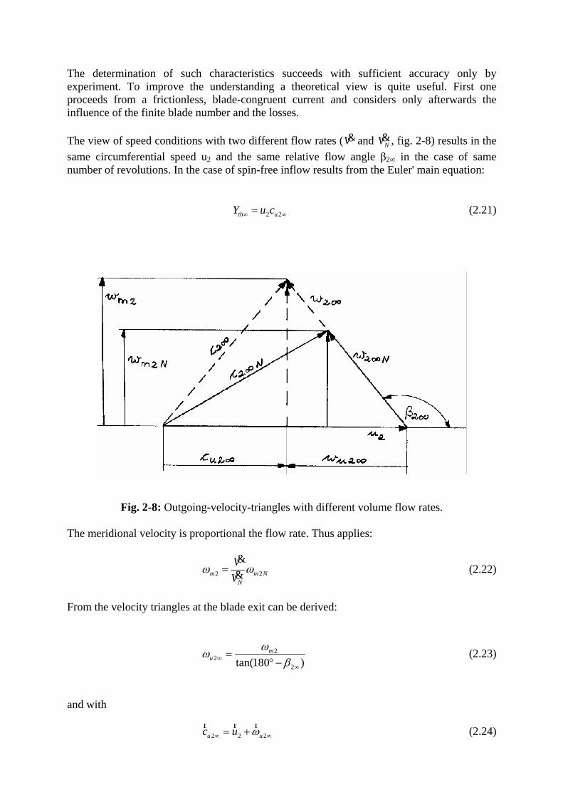
The determination of such characteristics succeeds with sufficient accuracy only by experiment. To improve the understanding a theoretical view is quite useful. First one proceeds from a frictionless, blade-congruent current and considers only afterwards the influence of the finite blade number and the losses. The view of speed conditions with two different flow rates (V& and , fig. 2-8) results in the same circumferential speed u

NV&

2 and the same relative flow angle β2∞ in the case of same number of revolutions. In the case of spin-free inflow results from the Euler' main equation:

2 2th uY u c∞ ∞= (2.21)

Fig. 2-8: Outgoing-velocity-triangles with different volume flow rates.

The meridional velocity is proportional the flow rate. Thus applies:

2mN

VV

ω ω=&& 2m N (2.22)

From the velocity triangles at the blade exit can be derived:

22

2tan(180 )m

uωω

β∞∞

=° −

(2.23)

and with

2 2uc u 2uω∞ = + ∞

rr r (2.24)

2 2 2uc u ω∞ = − u ∞

)

(2.25) derives

2 2 2(th uY u u ω∞ = − ∞ (2.26)

2 2 22

2 2tanm N

thN

uVY uV A

ωβ∞

∞

= +&& (2.27)

2 22

2 2tanthuY u V

A β∞∞

= + & (2.28)

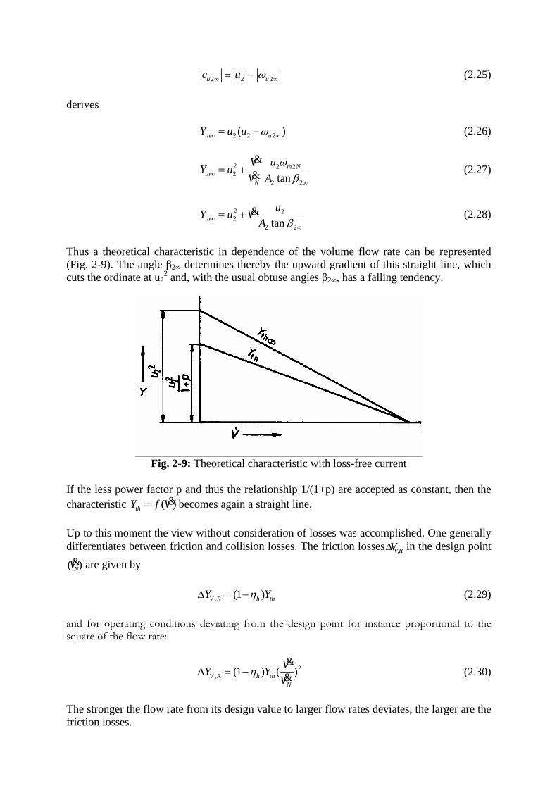
Thus a theoretical characteristic in dependence of the volume flow rate can be represented (Fig. 2-9). The angle β2∞ determines thereby the upward gradient of this straight line, which cuts the ordinate at u2

2 and, with the usual obtuse angles β2∞, has a falling tendency.

Fig. 2-9: Theoretical characteristic with loss-free current

If the less power factor p and thus the relationship 1/(1+p) are accepted as constant, then the characteristic becomes again a straight line. ( )thY f V= &

Up to this moment the view without consideration of losses was accomplished. One generally differentiates between friction and collision losses. The friction losses ,V RVΔ in the design point ( )NV& are given by

, (1 )V R h thY YηΔ = − (2.29) and for operating conditions deviating from the design point for instance proportional to the square of the flow rate:

2, (1 ) ( )V R h th

N

VY YV

ηΔ = −&& (2.30)

The stronger the flow rate from its design value to larger flow rates deviates, the larger are the friction losses.

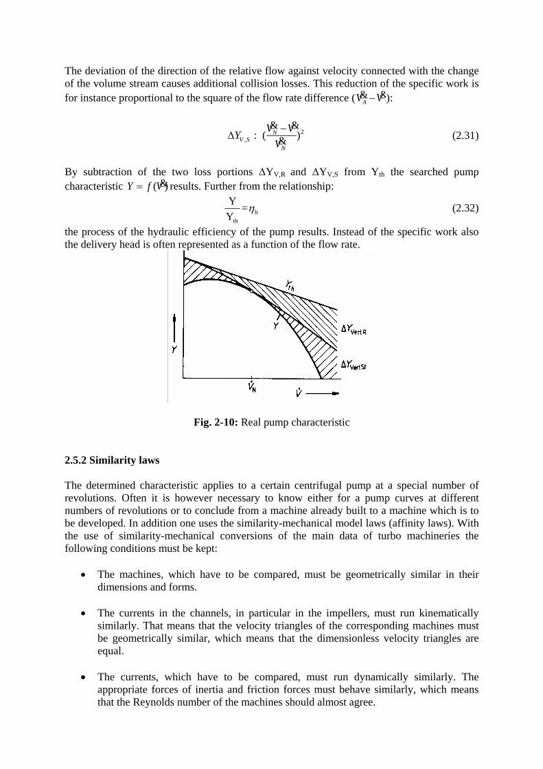
The deviation of the direction of the relative flow against velocity connected with the change of the volume stream causes additional collision losses. This reduction of the specific work is for instance proportional to the square of the flow rate difference ( AV V−& &):

2, ( N

V SN

V VYV−

Δ& &

: & ) (2.31)

By subtraction of the two loss portions ΔYV,R and ΔYV,S from Yth the searched pump characteristic results. Further from the relationship: ( )Y f V= &

hth

Y = Y

η (2.32)

the process of the hydraulic efficiency of the pump results. Instead of the specific work also the delivery head is often represented as a function of the flow rate.

Fig. 2-10: Real pump characteristic

2.5.2 Similarity laws The determined characteristic applies to a certain centrifugal pump at a special number of revolutions. Often it is however necessary to know either for a pump curves at different numbers of revolutions or to conclude from a machine already built to a machine which is to be developed. In addition one uses the similarity-mechanical model laws (affinity laws). With the use of similarity-mechanical conversions of the main data of turbo machineries the following conditions must be kept:

• The machines, which have to be compared, must be geometrically similar in their dimensions and forms.

• The currents in the channels, in particular in the impellers, must run kinematically

similarly. That means that the velocity triangles of the corresponding machines must be geometrically similar, which means that the dimensionless velocity triangles are equal.

• The currents, which have to be compared, must run dynamically similarly. The

appropriate forces of inertia and friction forces must behave similarly, which means that the Reynolds number of the machines should almost agree.

The comparison of two geometrically similar impellers a and b with same dimensionless velocity triangles results under the condition of spin-free incident flow and same efficiencies in the following connections: Delivery head

2 2uYH ug g

cη= = (2.33)

2, 2

2,

( ) (aa

b b

DHH D n

= 2)a

b

n (2.34)

Volume flow rate

2 2 2mV c D B π= ⋅ ⋅ ⋅& (2.35)

2, 3

2,

( aa a

b b b

DV nV n D

=&& ) (2.36)

Available power

P H g Vρ= ⋅ ⋅ ⋅ & (2.37)

2,3

2,

( ) ( )aa a

b b b

DP nP n D

= 5 (2.38)

The accepted equality of the efficiencies is only approximately correct, since as a result of change of the machine size, the number of revolutions or the viscosity of the delivery medium a deviation of the efficiency arises. The change of efficiency can be considered by so-called empirical revaluation formulas. By Pfleiderer applies:

0,11 Re( )1 Re

b a

a b

ηη

−=

− (2.39)

with

2 2Re u Dν⋅

= (2.40)

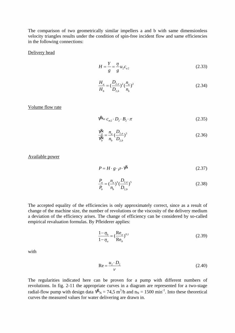
The regularities indicated here can be proven for a pump with different numbers of revolutions. In fig. 2-11 the appropriate curves in a diagram are represented for a two-stage radial-flow pump with design data V&N = 74,5 m3/h and nN = 1500 min-1. Into these theoretical curves the measured values for water delivering are drawn in.

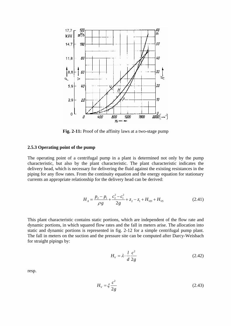
Fig. 2-11: Proof of the affinity laws at a two-stage pump

2.5.3 Operating point of the pump The operating point of a centrifugal pump in a plant is determined not only by the pump characteristic, but also by the plant characteristic. The plant characteristic indicates the delivery head, which is necessary for delivering the fluid against the existing resistances in the piping for any flow rates. From the continuity equation and the energy equation for stationary currents an appropriate relationship for the delivery head can be derived:

2 22 1 2 1

2 12Ap p c cH z z

g gρ− −

= + + − + +VD VSH H (2.41)

This plant characteristic contains static portions, which are independent of the flow rate and dynamic portions, in which squared flow rates and the fall in meters arise. The allocation into static and dynamic portions is represented in fig. 2-12 for a simple centrifugal pump plant. The fall in meters on the suction and the pressure site can be computed after Darcy-Weisbach for straight pipings by:

2

2Vl cHd g

λ= ⋅ (2.42)

resp.

2

2VcHg

ξ= (2.43)

;if one assumes that the dependence of the friction number for pipes λ and the coefficients of drag ξ on the Reynolds number and thus on the delivered flow V& is negligible .

Fig. 2-12: Plant characteristic

The operating point of the pump adjusts itself, where the delivery head of the centrifugal pump and the plant are the same size. That is the case in the intersection of pumping and plant characteristic. An extremely important condition for working the pump in the adjusting operating point is the demand:

NPSHgiven ≥ NPSHneeded (2.44) Only under keeping this condition a cavitation-free running is ensured. 2.5.4 Regulation of centrifugal pump plants With changing plant conditions a control procedure is released, with which the intersection of the two characteristics is shifted, until the requested flow rate is reached. In order to reach this, the following possibilities are available:

• Measures on sides of the plant

- Change of the dynamic portions of the plant characteristic through: , ( )A dynH f= &V· Throttling · Opening of bypasses in the pressure pipe

- Change of the static portion of the plant characteristic HA,stat through:

· Adapt the counter-pressure in the tank · Change of the geodetic differences in height of the water levels

• Measures on side of the pump

- Change of the pump parameters

· Number of revolutions · Positive Spin before the impeller by spin throttle or arranged bypass

· Rotor blade position · Switching on or off parallel-working pumps · Correction of the impeller diameter · Sharpen of the vane ends

• Measures on side of the medium

- Change of the middle density ρ of the delivery medium by steered content of steam bubbles (self-regulation by cavitation)

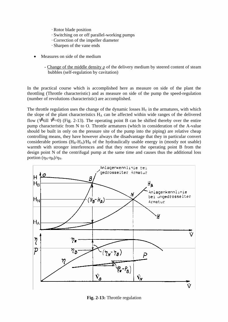
In the practical course which is accomplished here as measure on side of the plant the throttling (Throttle characteristic) and as measure on side of the pump the speed-regulation (number of revolutions characteristic) are accomplished. The throttle regulation uses the change of the dynamic losses HV in the armatures, with which the slope of the plant characteristics HA can be affected within wide ranges of the delivered flow (V&till V&=0) (Fig. 2-13). The operating point B can be shifted thereby over the entire pump characteristic from N to O. Throttle armatures (which in consideration of the A-value should be built in only on the pressure site of the pump into the piping) are relative cheap controlling means, they have however always the disadvantage that they in particular convert considerable portions (HB-HA)/HB of the hydraulically usable energy in (mostly not usable) warmth with stronger interferences and that they remove the operating point B from the design point N of the centrifugal pump at the same time and causes thus the additional loss portion (ηN-ηB)/ηN.

Fig. 2-13: Throttle regulation

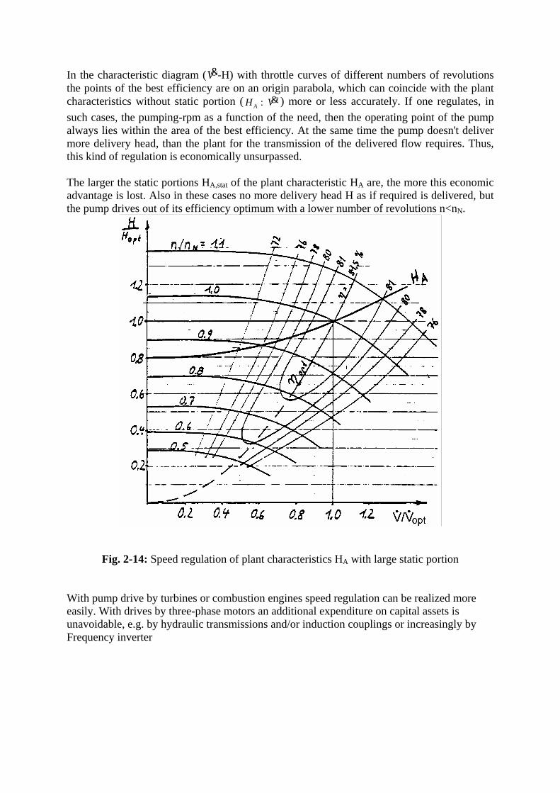
In the characteristic diagram (V&-H) with throttle curves of different numbers of revolutions the points of the best efficiency are on an origin parabola, which can coincide with the plant characteristics without static portion ( ) more or less accurately. If one regulates, in such cases, the pumping-rpm as a function of the need, then the operating point of the pump always lies within the area of the best efficiency. At the same time the pump doesn't deliver more delivery head, than the plant for the transmission of the delivered flow requires. Thus, this kind of regulation is economically unsurpassed.

2AH V&:

The larger the static portions HA,stat of the plant characteristic HA are, the more this economic advantage is lost. Also in these cases no more delivery head H as if required is delivered, but the pump drives out of its efficiency optimum with a lower number of revolutions n<nN.

Fig. 2-14: Speed regulation of plant characteristics HA with large static portion With pump drive by turbines or combustion engines speed regulation can be realized more easily. With drives by three-phase motors an additional expenditure on capital assets is unavoidable, e.g. by hydraulic transmissions and/or induction couplings or increasingly by Frequency inverter

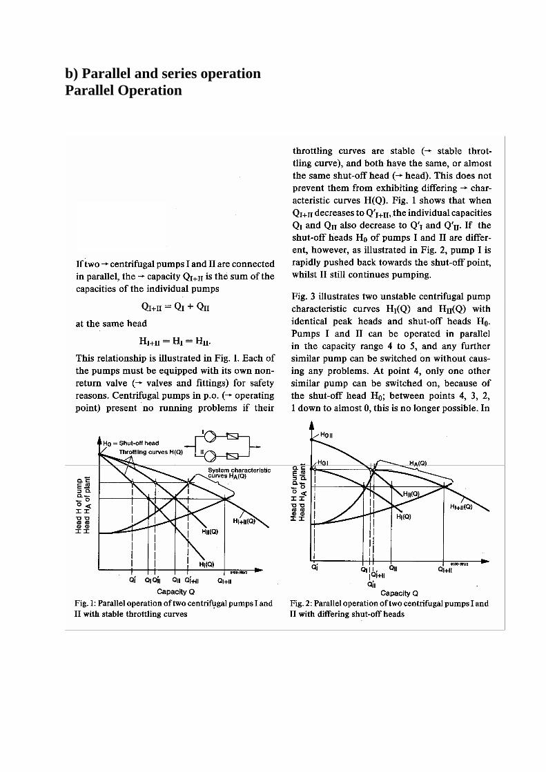
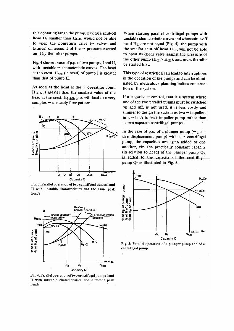
b) Parallel and series operation Parallel Operation

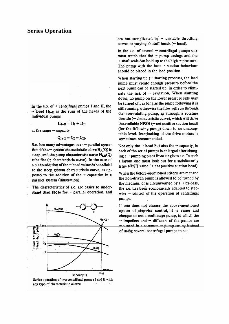
Series Operation

c) Example for parallel and series operation

APPARATUS FOR TEACHING PARALLEL AND SERIAL CENTRIFUGAL PUMP SYSTEMS

BENTO RODRIGUES PONTES-JÚNIOR (bento@bauru.unesp.br)

EDSON DEL RIO VIEIRA (delrio@dem.feis.unesp.br)

JOÃO BATISTA APARECIDO (jbaparec@dem.feis.unesp.br)

Departamento de Engenharia Mecânica

Faculdade de Engenharia de Ilha Solteira

Universidade Estadual Paulista

ABSTRACT

Pumps assembled in parallel or in serial systems are of practical importance having many

applications in several process plants. A good knowledge about such systems and their

performance characteristics by the engineering undergraduate students is crucial. It is

presented in this work the construction, test and use of an assembly for teaching the

association in parallel or in series of centrifugal pumps. The assembly is constructed in a way

that turning on some valves and turning off other ones the apparatus becomes a parallel pump

system or a serial one. In order to get the performance characteristics of that pump systems is

necessary to do experimental measurements of pressure at inlet and outlet of the pumps, the

flow rate through the pump system, and the electric current and voltage of the electric motors

driving the pumps. The pressures are measured using Bourdon-tube pressure gauges and the

electric current and voltage by using ammeter and voltmeter connected to the electric motors.

Flow rate measurement is done by using a calibrated orifice meter. After getting all this

measurements it is obtained the pump system characteristic curves and the efficiency for

operating in parallel or in series.

INTRODUCTION

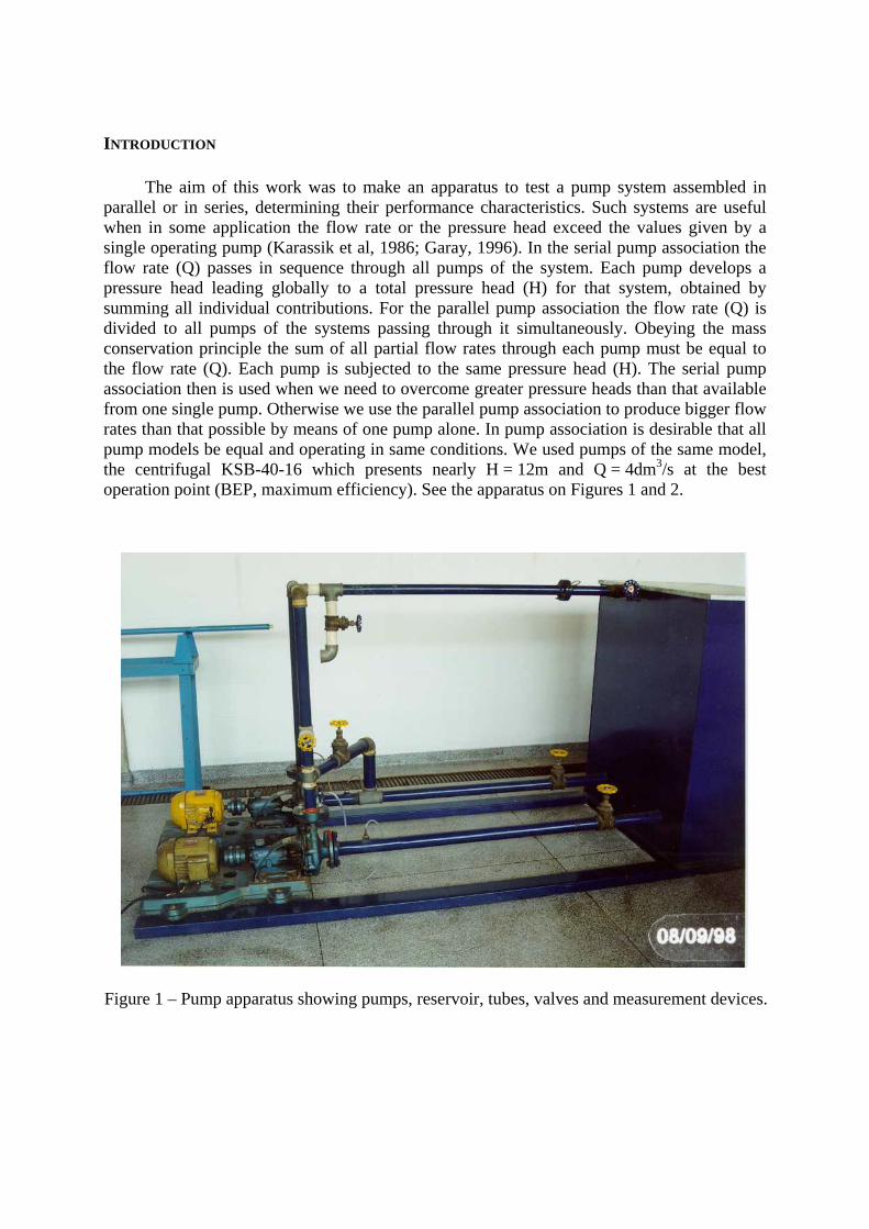
The aim of this work was to make an apparatus to test a pump system assembled in parallel or in series, determining their performance characteristics. Such systems are useful when in some application the flow rate or the pressure head exceed the values given by a single operating pump (Karassik et al, 1986; Garay, 1996). In the serial pump association the flow rate (Q) passes in sequence through all pumps of the system. Each pump develops a pressure head leading globally to a total pressure head (H) for that system, obtained by summing all individual contributions. For the parallel pump association the flow rate (Q) is divided to all pumps of the systems passing through it simultaneously. Obeying the mass conservation principle the sum of all partial flow rates through each pump must be equal to the flow rate (Q). Each pump is subjected to the same pressure head (H). The serial pump association then is used when we need to overcome greater pressure heads than that available from one single pump. Otherwise we use the parallel pump association to produce bigger flow rates than that possible by means of one pump alone. In pump association is desirable that all pump models be equal and operating in same conditions. We used pumps of the same model, the centrifugal KSB-40-16 which presents nearly H = 12m and Q = 4dm3/s at the best operation point (BEP, maximum efficiency). See the apparatus on Figures 1 and 2.

Figure 1 – Pump apparatus showing pumps, reservoir, tubes, valves and measurement devices.

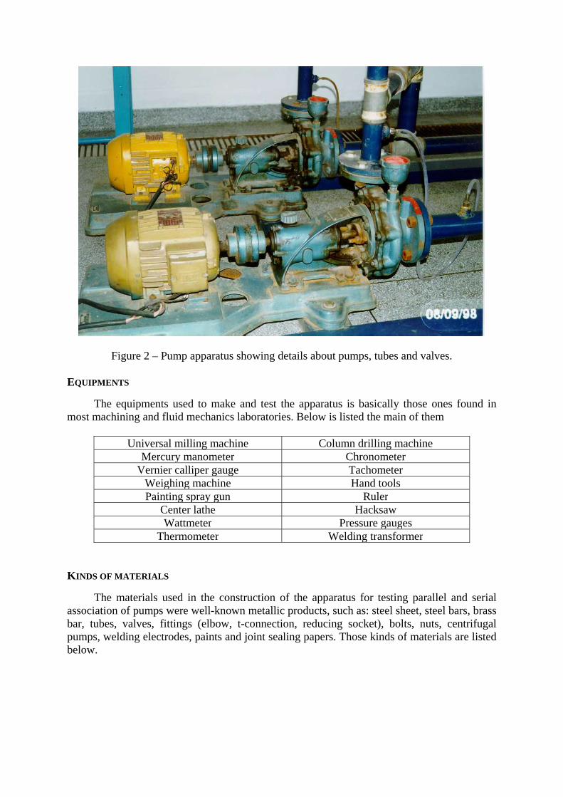
Figure 2 – Pump apparatus showing details about pumps, tubes and valves. EQUIPMENTS

The equipments used to make and test the apparatus is basically those ones found in most machining and fluid mechanics laboratories. Below is listed the main of them

Universal milling machine Column drilling machine

Mercury manometer Chronometer Vernier calliper gauge Tachometer

Weighing machine Hand tools Painting spray gun Ruler

Center lathe HacksawWattmeter Pressure gauges

Thermometer Welding transformer

KINDS OF MATERIALS

The materials used in the construction of the apparatus for testing parallel and serial association of pumps were well-known metallic products, such as: steel sheet, steel bars, brass bar, tubes, valves, fittings (elbow, t-connection, reducing socket), bolts, nuts, centrifugal pumps, welding electrodes, paints and joint sealing papers. Those kinds of materials are listed below.

Steel sheet – ABNT 1020 - 3×1220×2000 T-connection – 2”Steel tube – ABNT 1020 - φ1½” Elbow 90o - φ1½”Steel tube – ABNT 1020 - φ2” Reducing socket - φ2” - φ1½” Round steel bar – ABNT 1020 - φ6” Hexagonal-head bolt – M14×60 Round steel bar – ABNT 1020 - φ4” Hexagonal nut – M14Round steel bar – ABNT 1020 - φ1” Hexagonal-head bolt – M12×60 Hexagonal brass bar - φ½” Hexagonal nut – M12C-channel steel bar – ABNT 1020 – 4” Hexagonal-head bolt – M8×20 KSB® centrifugal pump – model 40-16 Hexagonal-head bolt – M8×40 Gate valve - φ2” Hexagonal nut – M8Gate valve - φ1½” Welding Electrodes Soldarc® 13 Globe valve - φ1½” PaintsT-connection - φ1½” Sealing paper

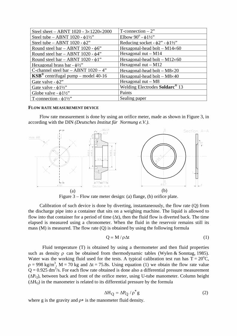
FLOW RATE MEASUREMENT DEVICE

Flow rate measurement is done by using an orifice meter, made as shown in Figure 3, in according with the DIN (Deutsches Institut für Normung e.V.).

(a) (b) Figure 3 – Flow rate meter design: (a) flange, (b) orifice plate.

Calibration of such device is done by diverting, instantaneously, the flow rate (Q) from

the discharge pipe into a container that sits on a weighing machine. The liquid is allowed to flow into that container for a period of time (Δt), then the fluid flow is diverted back. The time elapsed is measured using a chronometer. When the fluid in the reservoir remains still its mass (M) is measured. The flow rate (Q) is obtained by using the following formula

Q M t= / ρΔ (1)

Fluid temperature (T) is obtained by using a thermometer and then fluid properties such as density ρ can be obtained from thermodynamic tables (Wylen & Sonntag, 1985). Water was the working fluid used for the tests. A typical calibration test run has T = 20oC, ρ = 998 kg/m3, M = 70 kg and Δt = 75.8s. Using equation (1) we obtain the flow rate value Q = 0.925 dm3/s. For each flow rate obtained is done also a differential pressure measurement (ΔPQ), between back and front of the orifice meter, using U-tube manometer. Column height (ΔHQ) in the manometer is related to its differential pressure by the formula

Δ ΔH PQ Q= g∗/ ρ (2)

where g is the gravity and ρ∗ is the manometer fluid density.

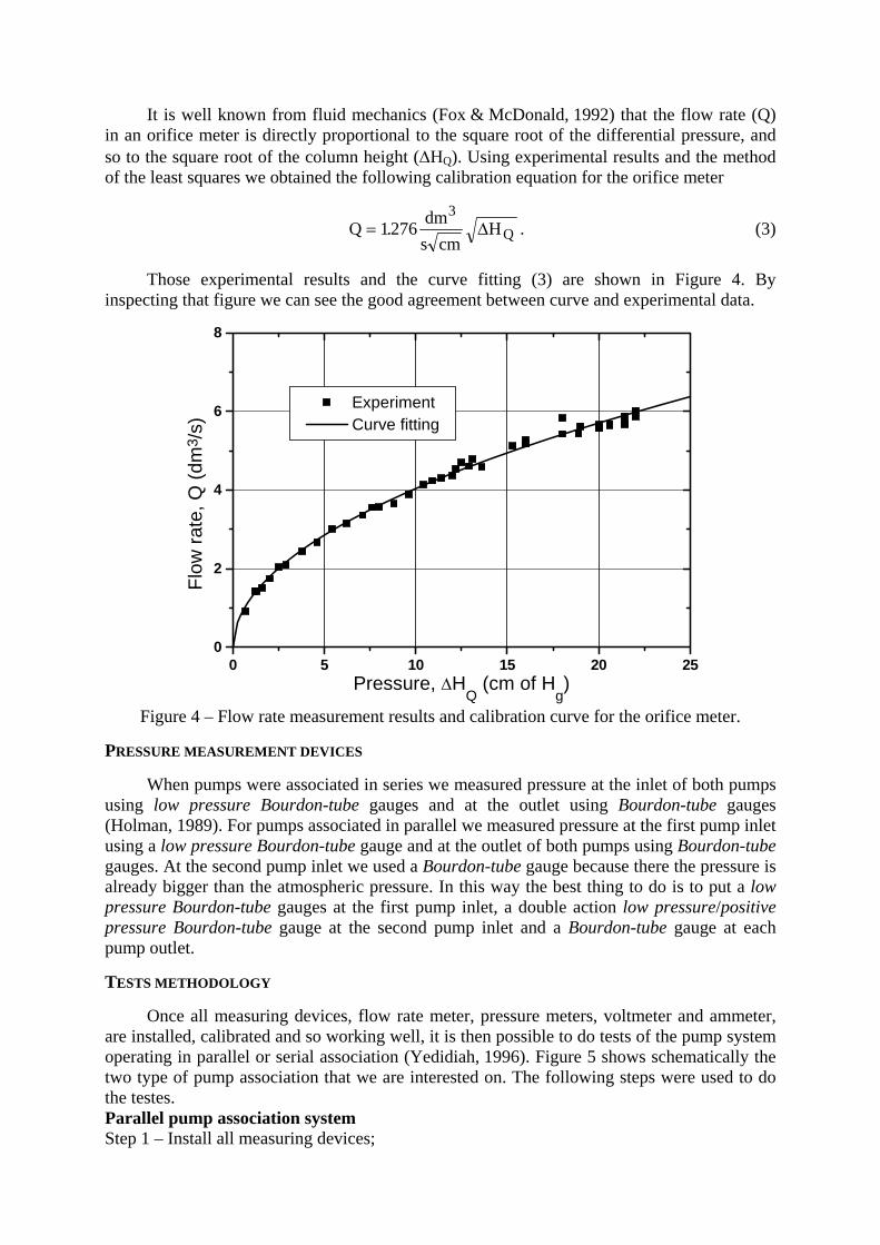
It is well known from fluid mechanics (Fox & McDonald, 1992) that the flow rate (Q) in an orifice meter is directly proportional to the square root of the differential pressure, and so to the square root of the column height (ΔHQ). Using experimental results and the method of the least squares we obtained the following calibration equation for the orifice meter

Q dms cm

HQ= 12763

. Δ . (3)

Those experimental results and the curve fitting (3) are shown in Figure 4. By inspecting that figure we can see the good agreement between curve and experimental data.

0 5 10 15 20 250

2

4

6

8

Experiment Curve fitting

Flow

rate

, Q (d

m3 /

s)

Pressure, ΔHQ

(cm of Hg)

Figure 4 – Flow rate measurement results and calibration curve for the orifice meter.

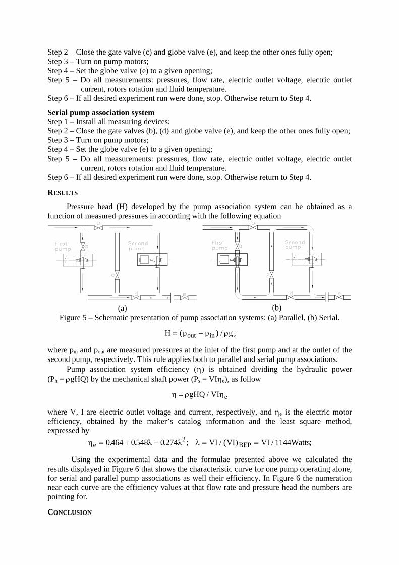
PRESSURE MEASUREMENT DEVICES When pumps were associated in series we measured pressure at the inlet of both pumps using low pressure Bourdon-tube gauges and at the outlet using Bourdon-tube gauges (Holman, 1989). For pumps associated in parallel we measured pressure at the first pump inlet using a low pressure Bourdon-tube gauge and at the outlet of both pumps using Bourdon-tube gauges. At the second pump inlet we used a Bourdon-tube gauge because there the pressure is already bigger than the atmospheric pressure. In this way the best thing to do is to put a low pressure Bourdon-tube gauges at the first pump inlet, a double action low pressure/positive pressure Bourdon-tube gauge at the second pump inlet and a Bourdon-tube gauge at each pump outlet. TESTS METHODOLOGY Once all measuring devices, flow rate meter, pressure meters, voltmeter and ammeter, are installed, calibrated and so working well, it is then possible to do tests of the pump system operating in parallel or serial association (Yedidiah, 1996). Figure 5 shows schematically the two type of pump association that we are interested on. The following steps were used to do the testes. Parallel pump association system Step 1 – Install all measuring devices;

Step 2 – Close the gate valve (c) and globe valve (e), and keep the other ones fully open; Step 3 – Turn on pump motors; Step 4 – Set the globe valve (e) to a given opening; Step 5 – Do all measurements: pressures, flow rate, electric outlet voltage, electric outlet

current, rotors rotation and fluid temperature. Step 6 – If all desired experiment run were done, stop. Otherwise return to Step 4.

Serial pump association system Step 1 – Install all measuring devices; Step 2 – Close the gate valves (b), (d) and globe valve (e), and keep the other ones fully open; Step 3 – Turn on pump motors; Step 4 – Set the globe valve (e) to a given opening; Step 5 – Do all measurements: pressures, flow rate, electric outlet voltage, electric outlet

current, rotors rotation and fluid temperature. Step 6 – If all desired experiment run were done, stop. Otherwise return to Step 4. RESULTS

Pressure head (H) developed by the pump association system can be obtained as a function of measured pressures in according with the following equation

(a) (b) Figure 5 – Schematic presentation of pump association systems: (a) Parallel, (b) Serial.

H p pout in g= −( ) / ρ ,

where pin and pout are measured pressures at the inlet of the first pump and at the outlet of the second pump, respectively. This rule applies both to parallel and serial pump associations. Pump association system efficiency (η) is obtained dividing the hydraulic power (Ph = ρgHQ) by the mechanical shaft power (Ps = VIηe), as follow

η ρ η= gHQ VI e/

where V, I are electric outlet voltage and current, respectively, and ηe is the electric motor efficiency, obtained by the maker’s catalog information and the least square method, expressed by

η λ λ λe BVI VI VI Watts= + − = =0 464 0548 0 274 11442. . . ; / ( ) /EP ;

Using the experimental data and the formulae presented above we calculated the results displayed in Figure 6 that shows the characteristic curve for one pump operating alone, for serial and parallel pump associations as well their efficiency. In Figure 6 the numeration near each curve are the efficiency values at that flow rate and pressure head the numbers are pointing for. CONCLUSION

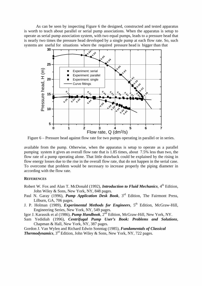
As can be seen by inspecting Figure 6 the designed, constructed and tested apparatus is worth to teach about parallel or serial pump associations. When the apparatus is setup to operate as serial pump association system, with two equal pumps, leads to a pressure head that is nearly two times the pressure head developed by a single pump at each flow rate. So, such systems are useful for situations where the required pressure head is bigger than that

0 1 2 3 4 5 6 75

10

15

20

25

300.5

9

0.62

0.65

0.66

0.65

0.63

0.61

0.58

0.56

0.52

0.48

0.39

0.50

0.55

0.64

0.68

0.680.6

8

0.66

0.660.6

5

0.160.33

0.490.53

0.580.60

0.620.63

Experiment: serial Experiment: parallel Experiment: single Curve fittings

Pre

ssur

e he

ad, H

(m)

Flow rate, Q (dm3/s) Figure 6 – Pressure head against flow rate for two pumps operating in parallel or in series.

available from the pump. Otherwise, when the apparatus is setup to operate as a parallel pumping system it gives an overall flow rate that is 1.85 times, about 7.5% less than two, the flow rate of a pump operating alone. That little drawback could be explained by the rising in flow energy losses due to the rise in the overall flow rate, that do not happen in the serial case. To overcome that problem would be necessary to increase properly the piping diameter in according with the flow rate. REFERENCES Robert W. Fox and Alan T. McDonald (1992), Introduction to Fluid Mechanics, 4th Edition,

John Wiley & Sons, New York, NY, 848 pages. Paul N. Garay (1996), Pump Application Desk Book, 3rd Edition, The Fairmont Press,

Lilburn, GA, 706 pages. J. P. Holman (1989), Experimental Methods for Engineers, 5th Edition, McGraw-Hill,

Engineering Series, New York, NY, 549 pages. Igor J. Karassik et al (1986), Pump Handbook, 2nd Edition, McGraw-Hill, New York, NY. Sam Yedidiah (1996), Centrifugal Pump User’s Book: Problems and Solutions,

Chapman & Hall, New York, NY, 387 pages. Gordon J. Van Wylen and Richard Edwin Sonntag (1985), Fundamentals of Classical Thermodynamics, 3rd Edition, John Wiley & Sons, New York, NY, 722 pages.

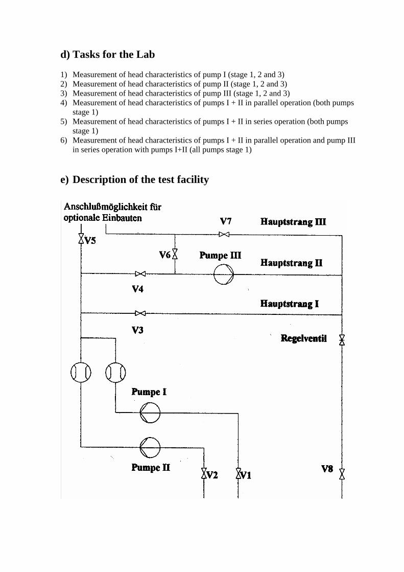
d) Tasks for the Lab

1) Measurement of head characteristics of pump I (stage 1, 2 and 3) 2) Measurement of head characteristics of pump II (stage 1, 2 and 3) 3) Measurement of head characteristics of pump III (stage 1, 2 and 3) 4) Measurement of head characteristics of pumps I + II in parallel operation (both pumps

stage 1) 5) Measurement of head characteristics of pumps I + II in series operation (both pumps

stage 1) 6) Measurement of head characteristics of pumps I + II in parallel operation and pump III

in series operation with pumps I+II (all pumps stage 1)

e) Description of the test facility

f) Report A report is required for this Lab work. In this report all measurement data have to be written down. The results for the tasks 1) to 6) should be presented in diagrams and extensively discussed.

g) Special Literature

1. Manual Centrifugal Pumps, pdf-File, see Download 2. Books about Centrifugal Pumps, see Library