ol

Study Habits and the Level of Alcoh Use Among College Students

Lisa M. Powell, PhDJenny Williams, PhDHenry Wechsler, PhD

February 2002

Research PaperImpacTeen is part of the BridgInforming Practice for Healthy The Robert Wood Johnson FouUniversity of Illinois at Chicago

Series, No. 19ing the Gap Initiative: ResearchYouth Behavior, supported byndation and administered by the

.

Study Habits and the Level of Alcohol UseAmong College Students

Lisa M. PowellQueen’s University and University of Illinois at Chicago

Jenny WilliamsUniversity of Adelaide and University of Illinois at Chicago

and

Henry WechslerHarvard University

Acknowledgements

We gratefully acknowledge research support from the Robert Wood Johnson Foundation toPowell and Williams through ImpacTeen (A Policy Research Partnership to Reduce YouthSubstance Use) and to Wechsler through the College Alcohol Study. The views expressedin this paper are those of the authors and do not necessarily reflect the views of the RobertWood Johnson Foundation. We thank Frank Chaloupka and Christina Ciecierski for theirhelpful suggestions. We are grateful to Yanjun Bao for her research assistance.

Copyright 2002 University of Illinois at Chicago

1

Abstract:This paper draws on the 1997 and 1999 waves of the College Alcohol Study to examinethe effect of alcohol consumption among college students on study habits. A two-stagegeneralized least squares estimation procedure is used to account for the potential correlationin the unobserved characteristics determining drinking behavior and study habits. Ourresults reveal that failing to account for the endogeneity of the level of drinking leads to anover-estimate of its effect on the likelihood that a student misses a class or gets behind inschool. We also find differential effects of drinking on the study habits of freshman studentsand their upper-year counterparts.

2

1 Introduction

The extent to which alcohol consumption impacts on both the quantity and quality of human

capital accumulation is an important question given that it has long run implications for

earnings. Following the human capital model developed by Becker (1964), an individual will

invest in acquiring additional levels of human capital based on the expected return in future

earnings. This decision takes into account both the costs of schooling and the rate at which

future benefits are discounted. At the same time, facing both budget and time constraints,

students make decisions about how much alcohol to consume.

The consumption of alcohol can be expected to have a negative impact on schooling both

directly through its potential impact on cognitive ability and indirectly through its impact

on study habits. A negative correlation between alcohol consumption and schooling also

may be observed, however, due to the fact that individuals who face high costs and/or place

a lower value on future earnings may invest less in schooling and at the same time these

individuals may be more likely to engage in heavy drinking behavior. Hence, controlling for

the potential endogeneity between drinking and schooling is of key importance in establishing

a causal link between alcohol use and schooling outcomes. Establishing such a casual link will

inform policy makers about the impact of alcohol policies on human capital accumulation and

the potential to reduce productivity losses associated with increased alcohol consumption.

The results from the existing literature that examines the impact of alcohol consumption

on educational attainment is mixed. Not surprisingly, studies that do not account for the po-

tential endogeneity between drinking and schooling measures find that alcohol consumption

significantly reduces schooling levels. In this regard, drawing on the National Longitudinal

Survey of Youth (NLSY), Yamada, Kendix and Yamada (1996) found that both the number

of liquor and wine drinks consumed during the past week and being a frequent drinker sig-

nificantly reduced the probability of high school graduation. A 10% increase the probability

of being a frequent drinker was found to reduce the likelihood of graduation by 6.5%. Also

without accounting for endogeneity, Mullahy and Sindelar (1994) used data from the Wave 1

of the New haven site of the National Institute of Mental Health Epidemiological Catchment

3

Area survey and found that alcoholic symptoms prior to age 22 reduced years of schooling

by 5%.

Among the studies that control for the possible correlation between the unobservables

that affect both drinking and schooling choice, the results range from significant to moderate

to no effect at all of youthful drinking on educational attainment. Using two-stage-least-

squares (2SLS) to account for endogeneity, Cook and Moore (1993) draw on the NLSY to

examine the effect of alcohol consumption (number of drinks per week, frequent drinking,

and being frequently drunk) on the years of post-secondary schooling. The authors found

that all three drinking measures significantly reduce years of schooling with frequent drinkers

completing 2.3 years less of college. Most recently, Koch and Ribar (2001) use data on same-

sex siblings from the 1979-90 NLSY to examine the effect of the age at which youths first

drank regularly on the number of years of schooling completed by age 25. Using a siblings IV

model, the results suggest that the effect of drinking onset is moderate – delaying drinking

for a year leads to 1/4 year of additional schooling.

However, drawing on 1977-92 Monitoring the Future data, Dee and Evans (1997) use

a two-sample instrumental variables procedure relying on within-state variation in their

instruments to examine the effect of being a drinker, moderate drinker, and heavy drinker

on high-school completion and college entrance and attainment. Overall, they find that

controlling for endogeneity, teen drinking does not have a significant effect on educational

attainment. Similarly, based on NLSY data, Chatterji (1998) finds that her estimation

results based on models that account for endogeneity reveal no significant effect of teen

alcohol consumption on the number of grades completed by age 21.

Most of this literature focuses on the educational outcomes related to prior teenage

drinking behavior. In this paper, we propose to focus on college-level educational outcomes

as a result of current drinking behavior. This is a particularly relevant issue, given that

alcohol is a common element in the environments of most college campuses (in 1999, the

annual alcohol prevalence rate among college students was 83.6% (Wechsler, Lee, Kuo and

Lee, 2000)).

Drawing on information available in the Harvard School of Public Health College Alcohol

4

Study (CAS), we provide evidence on the extent to which alcohol consumption impacts

on college study habits which in turn are expected to affect human capital accumulation.

Assessing the mechanisms through which alcohol consumption impacts schooling may shed

further light on the extent to which policies aimed at reducing alcohol consumption among

young adults may affect the quality and quantity of human capital accumulation. Current

evidence exists on the direct effect of drinking on cognitive ability. Based on clinical studies,

Nordby (1999) showed that drinking reduces recall which can be expected to have a direct

effect on schooling. However, we are not aware of existing empirical evidence of the effects

of alcohol consumption on indirect effects such as study habits.

We examine the impact of alcohol consumption defined by the average number of drinks

consumed per drinking occasion among college students who drink on the probability of

skipping a class and getting behind in school. We use a two-stage generalized least squares

estimation procedure to account for potential correlation in the unobservables that determine

drinking behavior and study habits. Generating consistent estimates of the effect of drinking

on college study habits requires an exogenous source of variation in college drinking. That is,

we require variables that affect college drinking levels but do not directly affect study habits.

In this regard, we use the price of alcohol, college-level information on access to alcohol, and

state-level alcohol policies to identify alcohol consumption. Our results reveal that given

the endogeneity of college drinking and study habits, single-stage estimation methods over-

estimate the true effect of the quantity of college drinking on the likelihood of missing a class

and getting behind in school. To further investigate the study habit behavior of our college

sample, we also estimate our model separately by year of class. We find differential effects

of drinking on the study habits of freshman and their upper-year counterparts.

Our paper is organized as follows. Section 2 describes our model of the relationship

between alcohol consumption and study habits. Section 3 describes our data and summary

statistics. Our estimation results are presented in section 4 and we conclude in section 5 with

a discussion of potential policy implications to improve study habits and reduce productivity

losses due to alcohol consumption among college students.

5

2 Model of Alcohol Use and Study Habits

This study examines the impact of alcohol consumption levels by college students on two

potential adverse study practices: skipping a class (SKIP) and getting behind in school

(BEHIND).1 A key goal of our empirical model is to establish a casual link between our

drinking measure and study habit outcomes. Hence, to control for the potential existence

of endogeneity between alcohol consumption and study habits, we estimate a two-stage

generalized least squares model.

We specify the probability of an adverse study habit practice as follows:

Hi = βDDi + β′XXi + εi (1)

where Di is the average number of alcohol drinks consumed, and Xi is a vector of individual

and college campus characteristics. In our model, the observed aspect of equation (1) of the

student’s study practices is a 0-1 dichotomous variable. A priori, we expect an increase in

alcohol consumption levels to increase the probability of an adverse study habit outcome.

The demand for alcohol consumption is specified as follows:

Di = βP Pi + β′CCi + β′

SSi + β′XXi + ui (2)

where Pi is the price of alcohol, the vector Ci includes campus measures related to access to

alcohol, the vector Si includes state-level alcohol-related policies, and the vector Xi includes

individual and college campus characteristics.

We begin by testing the exogeneity of our drinking measure using the Smith-Blundell ex-

ogeneity test.2 Having established that our drinking measure is endogenous, we implement

Amemiya’s Generalized Least Squares (AGLS) estimators for a dichotomous dependent vari-

1Due to data limitations, we are unable to examine the effect of drinking participation on our study habitoutcomes.

2Under the null hypothesis of this test, the model is appropriately specified with all explanatory variablesas exogenous. Under the alternative hypothesis, the suspected endogenous variable (in this case, our drink-ing measure) is expressed as linear projections of a set of instruments. The residuals from the first-stageregressions are added to the model and, under the null hypothesis, they should have no explanatory power.(Smith and Blundell, 1986)

6

able. In this model, the endogenous regressor, number of drinks, is treated as a linear function

of the instruments and the other exogenous variables. (Newey 1987) We use this two-stage

estimation method because it is likely that the error terms εi and ui are correlated – that is,

individuals who have an unobserved propensity to drink greater amounts of alcohol also may

be more likely to engage in behavior that adversely affects their human capital accumulation.

Hence, estimating equation (1) directly without implementing the first-stage estimation may

result in a biased and inconsistent estimate of the parameter βD in equation (1).

Our two-stage estimation procedure requires an exogenous source of variation in the

quantity of college drinking that does not directly affect study habits. In this regard, we

use the price of alcohol, college-level information on access to alcohol, and state-level alcohol

policies to identify alcohol consumption. To test the validity of our instruments, we estimate

a two-stage least squares (2SLS) model to perform the Davidson and MacKinnon (1993)

over-identification test.

Finally, to highlight the importance of controlling for endogeneity, we compare our re-

sults based on the AGLS model to single-stage probit results where the average number of

drinks consumed per drinking occasion is treated as an exogenous regressor. Also, to further

investigate the underlying behavior of our college sample, we estimate our model separately

by year of class.

3 Data Description

The data used for this analysis are drawn from the 1997 and 1999 waves of the College

Alcohol Study (CAS) conducted by the Harvard University School of Public Health.3 The

CAS student survey was administered to a random sample of full-time students at colleges

and universities from across the United States. The CAS is the first survey to focus on

drinking patterns in a nationally representative sample of college students. In 1997, 15,685

students from 130 colleges responded to the survey and, in 1999, 14,907 students from 128

3The first CAS was administered in 1993 but did not collect alcohol price data. Hence, we draw on the1997 and 1999 surveys.

7

colleges completed and returned the CAS student questionnaires.4 Table 2 provides detailed

summary statistics on the pooled 1997 and 1999 waves of the CAS data. Our sample contains

16756 observations based on a sub-sample of students who drank in the last 30 days and for

which we have non-missing data. We also provide sample means according to our adverse

study habit outcomes. The remainder of this section defines our dependent, independent,

and identifying variables.

3.1 Dependent variables:

We examine two possible adverse study habits based on self-reported information by students

who drank within the last year. The outcome measures are conditional on drinking – the

CAS only asked the study habit questions to those students who drank within the last year.

We construct 0-1 dichotomous dependent variables based on whether or not their drinking

resulted in the following outcomes: skipping a class (33%) or getting behind in school (28%).

As a measure of alcohol consumption we draw on the average consumption per drinking

occasion. The average consumption per drinking occasion measure is a continuous variable

that reflects the average number of drinks a student consumed per drinking occasion in the

previous 30 days. This variable is constructed from the following question: “In the past 30

days, on those occasions when you drank alcohol, how many drinks did you usually have?”.5

3.2 Independent variables:

The student surveys also obtained detailed demographic and socioeconomic information on

each of the respondents. This made it possible to construct controls for many of the other

important correlates. These variables include: the age of the respondent; an indicator for

gender; race (White - omitted, African American, Asian, Native American and Other race);

4See Wechsler, Davenport, Dowdall, Moeykens and Castillo (1994), Wechsler, Dowdall, Maenner, Gledhill-Hoyt and Lee (1998), and Wechsler, Lee, Kuo, and Lee (2000) for a detailed description of the samplingmethods and survey design of the CAS.

5It is worth re-iterating the point that given that the CAS only asked the study habit questions to thosestudents who drank within the last year, our estimation sample is conditional on drinking. Specifically, wesub-sample on those students who drank in the last 30 days as this reflects the best overlap between thestudy habit and drinking measures as permitted by the survey design.

8

ethnicity (Hispanic); marital status; religious affiliation (None or atheist - omitted, Catholic,

Judaism, Islam, Protestantism, Other); living arrangement (single sex residence hall, co-ed

residence hall, other university housing, fraternity/sorority housing, off-campus housing -

omitted, and other type of housing); current year in school (freshman - omitted, sophomore,

junior, senior, 5th year or beyond).

The CAS survey also obtained detailed background information on the parents of the

respondents. Parental information includes an indicator for parental education (at least one

parent attended college), as well as an indicator for both mothers’ and fathers’ past alcohol

use (defined separately for both mother and father: parent not present, parent is a former

problem drinker, parent abstains from alcohol - omitted, parent is an infrequent or moderate

drinker, parent is a heavy drinker or current problem drinker).

Finally, a key advantage of the CAS data set is that it contains an Administrators’

questionnaire. This allows us to include information on the type of campus (all female,

traditionally African-American, small private, large private, commuter campus, small public

or large public) and its regional location (South, West, Northeast or Midwest) in our analyses.

3.3 Identifying Variables:

In order to identify our drinking measure in our two-stage estimation procedure, we rely on

several variables that account for the full price of alcohol. First, we construct two college-

level price measures available for the first time in the student questionnaires of the 1997 and

1999 CAS surveys: the average real college price paid per alcoholic drink and the proportion

of students at a given college who pay a fixed fee for all they can drink. Students were

asked to report the amount that they typically pay for a single alcoholic drink. Possible

responses included: do not drink; pay nothing - drink free; under $.50; between $.51 and

$1.00; between $1.01 and $2.00; between $2.01 and $3.00; $3.01 or more; pay a set fee. Based

on this information, we construct the average college price as the campus mean of non-zero

prices (using mid-points) paid for a single alcoholic drink as reported by students from each

school. We use the consumer price index to denote our alcohol price measure in real 1990

9

dollars. The proportion of students who pay a fixed fee for all they can drink is defined as

the percentage of students who drink within each campus, who when asked about how much

they typically pay for a single alcoholic drink, reported typically paying a set fee to drink

alcohol. This latter measure allows us to account for the impact on alcohol consumption of

facing zero marginal cost after the first drink.

To further account for the full cost of alcohol, we include measures drawn from the CAS

Administrator questionnaires to construct variables that reflect access to alcohol at each

of the campuses. The first indicator equals one if there is a pub on campus and equals

zero otherwise. The second variable indicates if there is one or more outlets licensed to sell

alcoholic beverages located within one mile of the campus. We also take advantage of state-

level alcohol control laws that we merged with our CAS data. Our two state-level policy

variables capture information pertaining to whether or not the state imposes restrictions

(either regulation or prohibition of) on happy hours at bars and pubs and dram shop laws

which hold a bar or the owner of the establishment responsible for damages incurred from

heavy or excessive drinking. These measures are dichotomous indicators set equal to a value

of one if a state mandates a particular alcohol control policy and equal a value of zero

otherwise.

4 Results

We present our AGLS and probit model results of the impact of the average number of

alcohol drinks consumed on study habits for our full sample and by year in class in Table

1. We also report the p-value results from our Blundell-Smith exogeneity tests in Table 1.

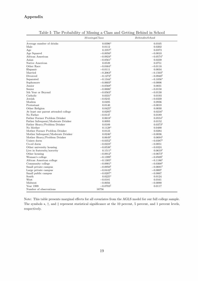
In the appendix, we present the results for all covariates based on the AGLS model; Table

I presents the results for the probability of missing a class and getting behind in school and

Table II presents the alcohol demand results. We begin by discussing our key findings and

then we highlight some of the detailed results from the full set of covariates presented in the

appendix.

Based on our full sample, our results reveal that with respect to study habits, the average

10

quantity of alcohol consumed per drinking occasion is endogenous. Hence, it is appropriate

to estimate a two-stage estimation model in order to account for the correlation in the unob-

servables. Based on our AGLS model, Table 1 shows that once we control for endogeneity,

an increase of an additional drink in the the average number of drinks consumed does not

significantly affect getting behind in school and only weakly (at the 10% level) reduces the

probability of skipping a class by about 4%. Based on the probit model, without correcting

for endogeneity, we would over-estimate the impact of an additional drink on the probability

of skipping a class and getting behind in school to be 8.9% and 5.4%, respectively.

To investigate the underlying behavior of students more closely, we estimate our model

separately by each class year. These results are quite interesting. We find that for freshman

students the observed correlation between drinking and study habits is driven by the corre-

lation in the unobservables. We reject exogeneity of our drinking measure at the 1% level

for missing a class and at the 10% level for getting behind in school. And, controlling for

endogeneity in our AGLS model, we find that the average amount drunk has no significant

impact on either of the two study habits. However, beyond the freshman year, the results

suggest that the drinking measure is exogenous (with the exception of drinking in the BE-

HIND model for juniors at the 10% level) and hence the probit results are valid which in

turn suggest that for the upper year classes an additional drink in the average amount drunk

increases the probability of missing a class by about 8-9% and getting behind in school by

about 5%.

Turning to our complete set of covariates for our full sample of college students, presented

in the appendix, we see from Table I that several of our individual/family and college control

variables are important determinants of college study habits, in particular for missing a class.

In terms of individual characteristics, we find that compared to their white counterparts,

African American students are less likely to miss a class or get behind in school, while Asians

and our other race category are also less likely to miss a class. Being married, divorced

or separated significantly reduces the probability of either of the two adverse outcomes.

Religious affiliation has no effect on getting behind in school, though being catholic increases

the likelihood of skipping a class. Older students are more likely to skip a class, while

11

compared to their freshman counterparts, controlling for age, upper year students are less

likely to skip a class. These latter variables do not significantly affect the probability of

getting behind in school. Finally, the living arrangements of students significantly affect

their study habit behavior. Compared to living off-campus, living on-campus in either a

dorm or other housing reduces the probability of skipping a class and living in a unisex dorm

or other housing reduces the probability of getting behind in school. Living in a fraternity

or sorority results in a strong significant increase in the probability of skipping a class and

getting behind in school, even after controlling for its effect on drinking behavior.

In terms of our parental characteristics, we find that having at least one parent who

attended college, significantly increases the probability of both of our adverse study habits.

While we might expect parents’ education levels (and hence income levels) to be positively

correlated with child educational outcomes, these results suggest that those students who

are first-generation college attendees are less likely to engage in activities that would under-

mine their educational attainment. First-generation college students may place more value

on their college opportunity compared to their counterparts who may take attending college

for granted. Similar to Chatterji (1998), we also find that parental alcoholism significantly

affects their children’s educational outcomes. Students with parents who fall into categories

of being a heavy or problem drinker or a former problem drinker are significantly more likely

to skip a class and get behind in school compared to their counterparts with parents who

are abstainers. Chatterji (1998) undertook sensitivity analyses with and without parental

alcoholism as a right hand side variable and found that after controlling for parental alco-

holism, adolescent substance use did not have a significant effect on schooling. Undertaking

similar sensitivity analyses, we find that our results are robust to the omission of the parental

alcohol variables.

Our results reveal that controlling for college characteristics is important. Compared

to their counterparts at a large public college, students who attend a women’s, African

American, commuter, or small private college are less likely to skip a class and get behind

in school. We find no significant difference among students who attend public (either small

or large) colleges or large (either public or private) colleges. Sensitivity analyses reveal

12

that omitting the college characteristics from our specification leads us to over-estimate the

impact of drinking on college study habits. Without including college characteristics in our

AGLS model, we find that the average number of drinks consumed per drinking occasion

significantly increases the probability of skipping a class and getting behind in school by

approximately 9% and 4%, respectively.

Turning to Table II, in the appendix, let us now examine the alcohol demand equation.

As noted earlier, in our two-stage AGLS estimation procedure, we identify our drinking

measure by the full cost of alcohol that includes the average price paid per drink, the fraction

of students who are able to purchase alcohol on a flat fee basis, college-level access measures,

and state-level alcohol policies.6 Our results reveal that, as expected, the price of alcohol

significantly reduces demand - a dollar increase in the average price reduces the average

number of drinks consumed per drinking occasion by 0.6 of a drink. Access to purchase

alcohol on a flat fee basis significantly increases the average number of drinks consumed by

1.6 drinks. Indeed this large effect is not surprising given that the flat fee drinking scheme

implies zero marginal monetary cost for each additional drink. We find that the presence of a

pub on campus or an alcohol outlet within one mile of campus does not significantly affect the

average number of drinks consumed by college students. We find that state dram shop laws

that hold establishments responsible for damages incurred from heavy or excessive drinking

significantly reduces alcohol consumption levels. The results from Table II also show that

alcohol consumption levels differ by race, marital status, religion, housing arrangements7 (in

particular, fraternity/sorority housing), parental drinking behavior, and type of college.

6The validity of our instruments is confirmed by the Davidson and MacKinnon (1993) over-identificationtest. The Chi-squared test statistics based on the 2SLS estimation of drinking and missing a class anddrinking and getting behind in school models, are 5.3963 Chi-sq( 5) with a P-value of 0.3694 and 2.168875Chi-sq( 5) with P-value of 0.8253, respectively.

7While among our six housing categories we specify off-campus student housing as a single category,previous work has examined differences among this group and has found that students who live off-campuswithout parents versus those who live off-campus with parents report a higher prevalence of alcohol use.(Kuo et al. 2001)

13

5 Conclusion

The results based on our full sample of college students reveal that once you control for

endogeneity, alcohol consumption levels of students who drink do not have a strong impact

on study habits – the average number of drinks consumed per drinking occasion does not

significantly affect getting behind in school and only weakly affects the probability of skip-

ping a class. However, estimating our model separately by each class year we find differential

effects of drinking on study habits between freshman and upper year students. Our results

show that the observed correlation between drinking and study habits for freshman is at-

tributable fully to the correlation in the unobservables but that beyond the freshman year

our drinking measure is exogenous and, for these years, an increase of an additional drink

in the average amount drunk increases the probability of missing a class by about 8-9% and

getting behind in school by about 5%. We also find that race, parental drinking habits, living

in a fraternity/sorority, and the type of college one attends to be important determinants of

study habit practices by college students. When interpreting our results, we must bear in

mind that our estimation is based on the average quantity of alcohol consumed conditional

on drinking and, hence, we cannot draw inferences for the full college population. Indeed,

we would expect an additional impact on study habits through the drinking participation

decision. Further, given that the CAS sample is representative of students enrolled at college

at the time of survey though does not include individuals who were previously enrolled but

may have already dropped out of college due to heavy drinking, our results will tend to

underestimate the adverse effect of drinking on study habits.

Overall, our results show that reducing alcohol consumption levels among college students

may result in improved study habits among upper year students. Based on our alcohol

demand results, policymakers at both the state-level and school administrator level may

be successful in reducing alcohol consumption by several means. First, at the state-level,

increasing the price of alcohol via taxes and the imposition of dram shop laws across all

states can be expected to reduce drinking levels by college students. Second, we find that

college administrators could substantially reduce alcohol consumption levels among their

14

students by prohibiting the sale of alcohol on a flat fee basis. Further, the imposition of

local ordinances to prohibit the sale of alcohol on a flat fee basis would help to reduce

drinking levels both on and off-campus.

Indeed, the implementation of such policies to improve study habits can be expected to

improve both the quantity of education through an increased likelihood of college graduation

and the quality of schooling with students graduating with a better understanding of their

major. In turn, these human capital benefits can be expected to yield increases in long-run

earnings and reduce alcohol-related productivity losses.

15

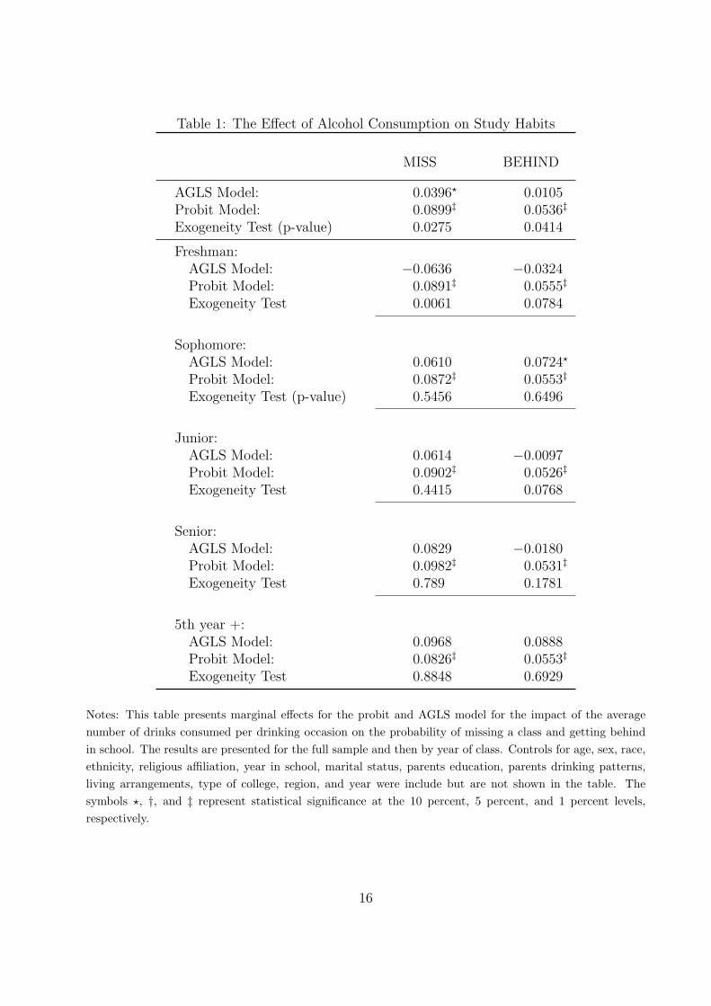
Table 1: The Effect of Alcohol Consumption on Study Habits

MISS BEHIND

AGLS Model: 0.0396? 0.0105Probit Model: 0.0899‡ 0.0536‡

Exogeneity Test (p-value) 0.0275 0.0414

Freshman:AGLS Model: −0.0636 −0.0324Probit Model: 0.0891‡ 0.0555‡

Exogeneity Test 0.0061 0.0784

Sophomore:AGLS Model: 0.0610 0.0724?

Probit Model: 0.0872‡ 0.0553‡

Exogeneity Test (p-value) 0.5456 0.6496

Junior:AGLS Model: 0.0614 −0.0097Probit Model: 0.0902‡ 0.0526‡

Exogeneity Test 0.4415 0.0768

Senior:AGLS Model: 0.0829 −0.0180Probit Model: 0.0982‡ 0.0531‡

Exogeneity Test 0.789 0.1781

5th year +:AGLS Model: 0.0968 0.0888Probit Model: 0.0826‡ 0.0553‡

Exogeneity Test 0.8848 0.6929

Notes: This table presents marginal effects for the probit and AGLS model for the impact of the averagenumber of drinks consumed per drinking occasion on the probability of missing a class and getting behindin school. The results are presented for the full sample and then by year of class. Controls for age, sex, race,ethnicity, religious affiliation, year in school, marital status, parents education, parents drinking patterns,living arrangements, type of college, region, and year were include but are not shown in the table. Thesymbols ?, †, and ‡ represent statistical significance at the 10 percent, 5 percent, and 1 percent levels,respectively.

16

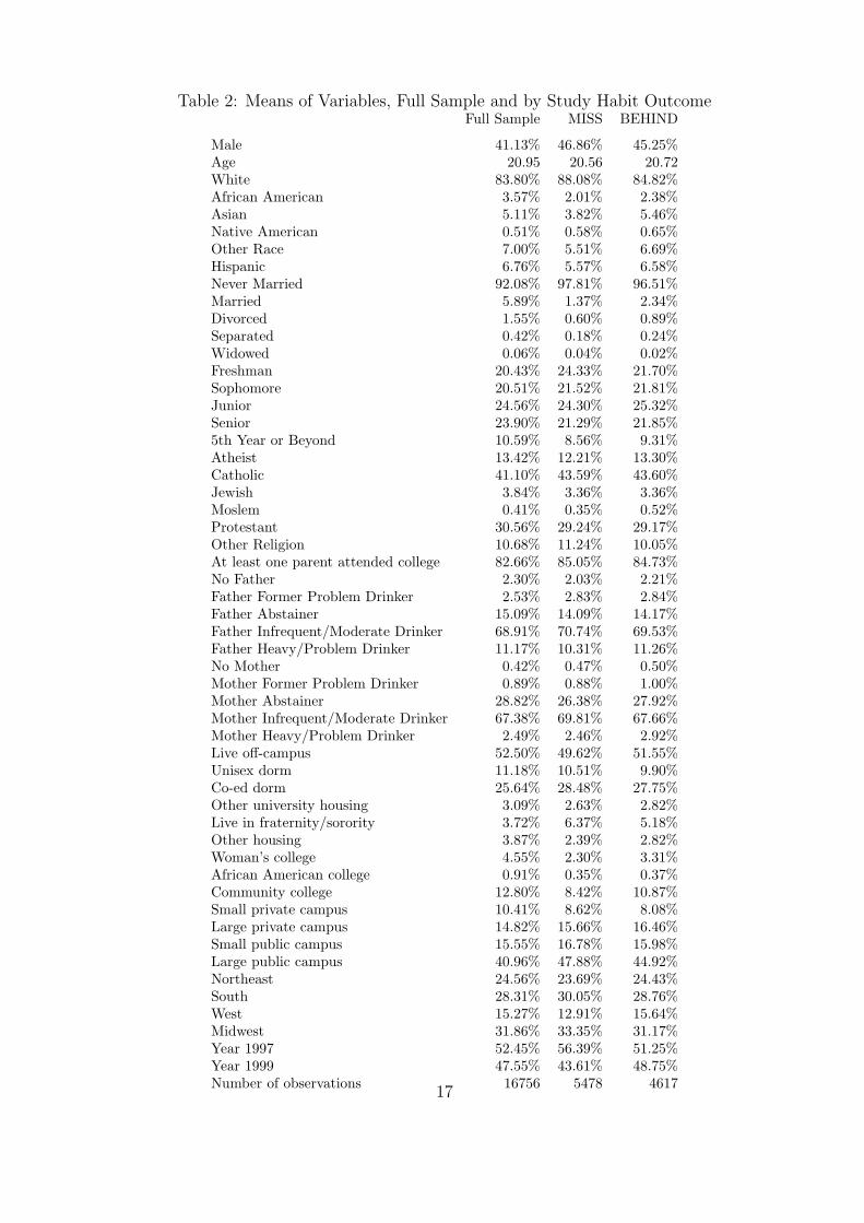
Table 2: Means of Variables, Full Sample and by Study Habit OutcomeFull Sample MISS BEHIND

Male 41.13% 46.86% 45.25%Age 20.95 20.56 20.72White 83.80% 88.08% 84.82%African American 3.57% 2.01% 2.38%Asian 5.11% 3.82% 5.46%Native American 0.51% 0.58% 0.65%Other Race 7.00% 5.51% 6.69%Hispanic 6.76% 5.57% 6.58%Never Married 92.08% 97.81% 96.51%Married 5.89% 1.37% 2.34%Divorced 1.55% 0.60% 0.89%Separated 0.42% 0.18% 0.24%Widowed 0.06% 0.04% 0.02%Freshman 20.43% 24.33% 21.70%Sophomore 20.51% 21.52% 21.81%Junior 24.56% 24.30% 25.32%Senior 23.90% 21.29% 21.85%5th Year or Beyond 10.59% 8.56% 9.31%Atheist 13.42% 12.21% 13.30%Catholic 41.10% 43.59% 43.60%Jewish 3.84% 3.36% 3.36%Moslem 0.41% 0.35% 0.52%Protestant 30.56% 29.24% 29.17%Other Religion 10.68% 11.24% 10.05%At least one parent attended college 82.66% 85.05% 84.73%No Father 2.30% 2.03% 2.21%Father Former Problem Drinker 2.53% 2.83% 2.84%Father Abstainer 15.09% 14.09% 14.17%Father Infrequent/Moderate Drinker 68.91% 70.74% 69.53%Father Heavy/Problem Drinker 11.17% 10.31% 11.26%No Mother 0.42% 0.47% 0.50%Mother Former Problem Drinker 0.89% 0.88% 1.00%Mother Abstainer 28.82% 26.38% 27.92%Mother Infrequent/Moderate Drinker 67.38% 69.81% 67.66%Mother Heavy/Problem Drinker 2.49% 2.46% 2.92%Live off-campus 52.50% 49.62% 51.55%Unisex dorm 11.18% 10.51% 9.90%Co-ed dorm 25.64% 28.48% 27.75%Other university housing 3.09% 2.63% 2.82%Live in fraternity/sorority 3.72% 6.37% 5.18%Other housing 3.87% 2.39% 2.82%Woman’s college 4.55% 2.30% 3.31%African American college 0.91% 0.35% 0.37%Community college 12.80% 8.42% 10.87%Small private campus 10.41% 8.62% 8.08%Large private campus 14.82% 15.66% 16.46%Small public campus 15.55% 16.78% 15.98%Large public campus 40.96% 47.88% 44.92%Northeast 24.56% 23.69% 24.43%South 28.31% 30.05% 28.76%West 15.27% 12.91% 15.64%Midwest 31.86% 33.35% 31.17%Year 1997 52.45% 56.39% 51.25%Year 1999 47.55% 43.61% 48.75%Number of observations 16756 5478 4617

17

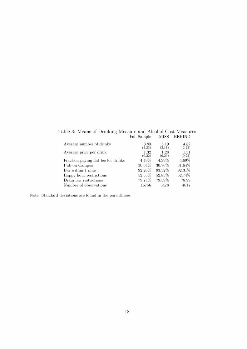
Table 3: Means of Drinking Measure and Alcohol Cost MeasuresFull Sample MISS BEHIND

Average number of drinks 3.83 5.19 4.82(2.23) (2.11) (2.22)

Average price per drink 1.32 1.28 1.31(0.22) (0.20) (0.22)

Fraction paying flat fee for drinks 4.49% 4.99% 4.69%Pub on Campus 30.64% 30.76% 31.64%Bar within 1 mile 92.26% 93.32% 92.31%Happy hour restrictions 52.55% 52.85% 52.74%Dram law restrictions 79.74% 79.59% 78.99Number of observations 16756 5478 4617

Note: Standard deviations are found in the parentheses.

18

Appendix

Table I: The Probability of Missing a Class and Getting Behind in SchoolMissingaClass BehindinSchool

Average number of drinks 0.0396? 0.0105Male 0.0112 0.0202Age 0.2357‡ 0.0373Age Squared −0.0056‡ −0.0010African American −0.0924‡ −0.0574†

Asian −0.0561† 0.0239Native American 0.0539 0.0751Other Race −0.0464† −0.0118Hispanic −0.0111 0.0034Married −0.2063‡ −0.1503‡

Divorced −0.1272‡ −0.0940‡

Separated −0.1344† −0.1056?

Sophomore −0.0603‡ −0.0006Junior −0.0568‡ 0.0031Senior −0.0606† −0.01585th Year or Beyond −0.0563† −0.0130Catholic 0.0331† 0.0193Jewish −0.0245 −0.0339Moslem 0.0495 0.0936Protestant 0.0140 −0.0018Other Religion 0.0425† 0.0030At least one parent attended college 0.0295‡ 0.0216†

No Father −0.0147 0.0189Father Former Problem Drinker 0.0618† 0.0554†

Father Infrequent/Moderate Drinker 0.0093 0.0152Father Heavy/Problem Drinker 0.0189 0.0373‡

No Mother 0.1128? 0.0490Mother Former Problem Drinker 0.0123 0.0284Mother Infrequent/Moderate Drinker 0.0246† −0.0036Mother Heavy/Problem Drinker 0.0649† 0.0694‡

Unisex dorm −0.0352† −0.0387‡

Co-ed dorm −0.0223† −0.0051Other university housing −0.0538† −0.0324Live in fraternity/sorority 0.1511‡ 0.0619†

Other housing −0.0912‡ −0.0673‡

Woman’s college −0.1399‡ −0.0509†

African American college −0.1305‡ −0.1186‡

Community college −0.0901‡ −0.0368‡

Small private campus −0.0950‡ −0.0691‡

Large private campus −0.0442‡ −0.0007Small public campus −0.0207? −0.0067South 0.0225? 0.0124West −0.0181 0.0161Midwest −0.0056 −0.0090Year 1999 −0.0703‡ 0.0117Number of observations 16756

Note: This table presents marginal effects for all covariates from the AGLS model for our full college sample.The symbols ?, †, and ‡ represent statistical significance at the 10 percent, 5 percent, and 1 percent levels,respectively.

19

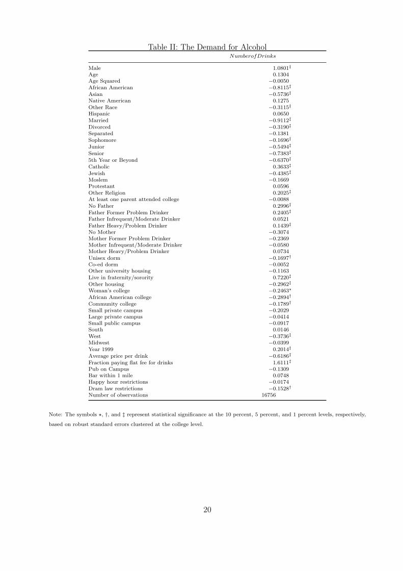
Table II: The Demand for AlcoholNumberofDrinks

Male 1.0801‡

Age 0.1304Age Squared −0.0050African American −0.8115‡

Asian −0.5736‡

Native American 0.1275Other Race −0.3115‡

Hispanic 0.0650Married −0.9112‡

Divorced −0.3190‡

Separated −0.1381Sophomore −0.1696‡

Junior −0.5494‡

Senior −0.7383‡

5th Year or Beyond −0.6370‡

Catholic 0.3633‡

Jewish −0.4385‡

Moslem −0.1669Protestant 0.0596Other Religion 0.2025‡

At least one parent attended college −0.0088No Father 0.2996‡

Father Former Problem Drinker 0.2405‡

Father Infrequent/Moderate Drinker 0.0521Father Heavy/Problem Drinker 0.1439‡

No Mother −0.3074Mother Former Problem Drinker −0.2369Mother Infrequent/Moderate Drinker −0.0580Mother Heavy/Problem Drinker 0.0734Unisex dorm −0.1697†

Co-ed dorm −0.0052Other university housing −0.1163Live in fraternity/sorority 0.7220‡

Other housing −0.2962‡

Woman’s college −0.2463?

African American college −0.2894†

Community college −0.1789†

Small private campus −0.2029Large private campus −0.0414Small public campus −0.0917South 0.0146West −0.3736‡

Midwest −0.0399Year 1999 0.2014‡

Average price per drink −0.6186‡

Fraction paying flat fee for drinks 1.6111‡

Pub on Campus −0.1309Bar within 1 mile 0.0748Happy hour restrictions −0.0174Dram law restrictions −0.1528†

Number of observations 16756

Note: The symbols ?, †, and ‡ represent statistical significance at the 10 percent, 5 percent, and 1 percent levels, respectively,

based on robust standard errors clustered at the college level.

20

References

Becker, Gary (1964). Human Capital. New York: National Bureau of Economic Research.

Chatterji, Pinks (1998). Does use of alcohol and illicait drugs during adolescence affect edu-cational attainment?: Results from three estimation methods. Unpublished Manuscript.

Cook, Philip J. and Michael J. Moore (1993). Drinking and schooling. Journal of HealthEconomics 12, 411–429.

Davidson, Russell and James G. MacKinnon (1993). Estimation and Inference in Economet-rics. New York: Oxford University Press.

Dee, Thomas S. and William N. Evans (1997). Teen drinking and educational attainment:Evidence from two-sample instrumental variables (TSIV) estimates. NBER WorkingPaper No. 6082.

Koch, Steven F. and David C. Ribar (2001). A siblings analysis of the effects of alcoholconsumption onset on educational attainment. Contemporary Economic Policy 19(2),162–74.

Kuo, Meichun, Edward M. Adlaf, Hang Lee, Louis Gliksman, Andree Demers, and HenryWechsler (2002). More canadian students drink but american students drink more: Com-paring college alcohol use in two countries.

Mullahy, J. and J. L. Sindelar (1994). Alcoholism and income: The role of indirect effects.Milbank Quarterly 72(2), 359–75.

Newey, W. (1987). Efficient estimation of limited dependent variable models with endogenousexplanatory variables. Journal of Econometrics 36, 231–50.

Nordby, Knut, Reidulf G. Watten, Ruth Kjaersti Raanaas, and Svein Magnussen (1999).Effects of moderate doses of alcohol on immediate recall of numbers: Some implicationsfor information technology. Journal of Studies on Alcohol 60(6), 873–78.

Smith, Richard, J. and Richard W. Blundell (1986). An exogeneity test for a simultaneousequation tobit model with an application to labor supply. Econometrica 54, 679–86.

Wechsler, H., A. Davenport, G. Dowdall, B. Moekens, and S. Castillo (1994). Health andbehavioral consequences of binge drinking in college: A national survey of students at140 campuses. Journal of the American Medical Association 272, 1672–1677.

Wechsler, Henry, George W. Dowdall, G. Maenner, J. Gledhill-Hoyt, and H. Lee (1998).Changes in binge drinking and related problems among american college students be-tween 1993 and 1997. Journal of American College Health 47, 57–68.

Wechsler, Henry, Jae Eun Lee, Meichun Kuo, and Hang Lee (2000). College binge drinkingin the 1990s: A continuing problem. Journal of American College Health 48, 199–210.

Yamada, Tetsuji, Michael Kendix, and Tadashi Yamada (1996). The impact of alcohol con-sumption and marijuana use on high school graduation. Health Economics 5, 77–92.

21

For these and other papers in the series, please visit www.impacteen.org

Recent ImpacTeen and YES! Research Papers

Effects of Price and Access Laws on Teenage Smoking Initiation: A National LongitudinalAnalysis, Tauras JA, O’Malley PM, Johnston LD, April 2001.

Marijuana and Youth, Pacula R, Grossman M, Chaloupka F, O’Malley P, Johnston L, Farrelly M,October 2000.

Recent ImpacTeen Research Papers

Study Habits and the Level of Alcohol Use Among College Students, Powell LM, Williams J,Wechsler H, February 2002.

Does Alcohol Consumption Reduce Human Capital Accumulation? Evidence from the CollegeAlcohol Study, Williams J, Powell LM, Wechsler H, February 2002.

Habit and Heterogeneity in College Students’ Demand for Alcohol, Williams J, January 2002.

Are There Differential Effects of Price and Policy on College Students’ Drinking Intensity?Williams J, Chaloupka FJ, Wechsler H, January 2002.

Alcohol and Marijuana Use Among College Students: Economic Complements or Substitutes?Williams J, Pacula RL, Chaloupka FJ, Wechsler H, November 2001.

The Drugs-Crime Wars: Past, Present and Future Directions in Theory, Policy and ProgramInterventions, McBride DC, VanderWaal CJ, Terry-McElrath, November 2001.

State Medical Marijuana Laws: Understanding the Laws and their Limitations, Pacula RL,Chriqui JF, Reichmann D, Terry-McElrath YM, October 2001.

The Impact of Prices and Control Policies on Cigarette Smoking among College Students, CzartC, Pacula RL, Chaloupka FJ, Wechsler H, March 2001.

Youth Smoking Uptake Progress: Price and Public Policy Effects, Ross H, Chaloupka FJ,Wakefield M, February 2001.

Adolescent Patterns for Acquisition and Consumption of Alcohol, Tobacco and Illicit Drugs: AQualitative Study, Slater S, Balch G, Wakefield M, Chaloupka F, February 2001.

State Variation in Retail Promotions and Advertising for Marlboro Cigarettes, Slater S,Chlaoupka FJ, Wakefield M, February 2001

The Effect of Public Policies and Prices on Youth Smoking, Ross H, Chaloupka FJ, February2001.

The Effect of Cigarette Prices on Youth Smoking, Ross H, Chaloupka FJ, February 2001.

Differential Effects of Cigarette Price on Youth Smoking Intensity, Liang L, Chaloupka FJ,February 2001.

ImpacTeen

Coordinating Center

University of Illinois at Chicago

Frank Chaloupka, PhD

www.uic.edu/orgs/impacteen

Health Research and Policy Centers

850 West Jackson Boulevard

Suite 400 (M/C 275)

Chicago, Illinois 60607

312.413.0475 phone

312.355.2801 fax

State Alcohol ResearchUniversity of MinnesotaAlexander Wagenaar, PhDwww.epl.umn.edu/alcohol

State Tobacco ResearchRoswell Park Cancer InstituteGary Giovino, PhDwww.roswellpark.org

State Illicit Drug ResearchAndrews UniversityDuane McBride, PhDwww.andrews.edu